Clustering. How are we doing on the pass sequence? Pretty good! We can now automatically learn the...
47
Clustering
-
Upload
cody-little -
Category
Documents
-
view
213 -
download
0
Transcript of Clustering. How are we doing on the pass sequence? Pretty good! We can now automatically learn the...

Clustering

How are we doing on the pass sequence?
Pretty good! We cannow automatically learnthe features needed totrack both people
But, it sucks that we need to hand-label the coordinates of both men in 30 frames and hand-label the 2 classes for the white-shirt tracker
Same set of weights used for all hidden units

Unsupervised learning
• Goal: Learn a machine or model that explains the data using a predefined set of assumptions about how the explanations can work
• There isn’t any labeled data, just input patterns (ie, instead of x,t-pairs, we have only x’s)
• Examples of unsupervised learning– Clustering (eg, k-means clustering)– Dimensionality reduction (eg, PCA)– Data compression methods (eg, ZIP, JPEG, MPEG)– Generative models & Bayesian networks (tomorrow)
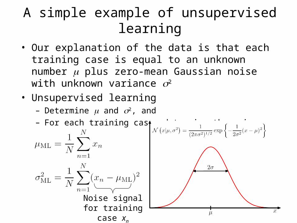
A simple example of unsupervised learning
• Our explanation of the data is that each training case is equal to an unknown number plus zero-mean Gaussian noise with unknown variance 2
• Unsupervised learning– Determine and 2, and– For each training case, determine the noise signal
Noise signal for training case xn

A simple example of unsupervised learning• What can this model be used for?• Outlier detection / novelty detection
– Given a new input xN+1, define p as follows (see figure)
If xN+1 < let p = z=-∞
xN+1 N(z|,2)dz and otherwise
let p = z=xN+1
∞ N(z|,2)dz
– Then, we can say that the new input xN+1 is an outlier (“unusual”) if p < 0.01
• Preference prediction– Given a set of new inputs,
we can rank them
according to probabilityxN+1

Problem
Training data
Gaussian estimated from training data
This test case has higher density than any of the
training cases, but is quite probably an outlier

K-means clusteringData and
initial (random)
means
Set each mean to the average of its
data
Assign each point to its nearest
meanIteration
1
Iteration 2
Iteration 3
Iteration 4 and
convergence

K-means clustering• Suppose x1,…,xN are real-valued or vector-valued
• Goal: Learn K means and assign each training case to a mean
• Denote the means by 1,…, K
• Use one-of-K encoding for the assignments:
rnk = 1 if xn is assigned to k, and rnk = 0 otherwise
• The goal of k-means clustering is to find the r’s and ’s that minimize the following cost function:
• Generally, finding an exact solution takes time that is exponential in N

K-means clustering
• Note that given the ’s we can efficiently find the best r’s, and given the r’s, we can efficiently find the best ’s
• Here’s the algorithm:
Pick initial means randomly or cleverlyLoop until convergence– Assign each training case to its nearest mean:
– Set each mean to the average of its training cases:
• Each step minimizes J wrt the r’s or the ’s, but the procedure is not guaranteed to find the minimum of J

Example Data and initial
(random) means
Set each mean to the average of its
data
Assign each point to its nearest
meanIteration
1
Iteration 2
Iteration 3
Iteration 4 and
convergenceIteration

Example: Color quantization
• Consider each image pixel as a 3-D vector (RGB) and use K-means clustering to find K “prototype colors”
• Now, each pixel in the image can be stored using log2(K) bits, with some loss in color quality
1 bit per pixel24 bits per pixel 1.6 bits per pixel 3.3 bits per pixel

EM for a mixture of Gaussians
• Initialization: Pick ’s, ’s, ’s randomly but validly• E Step: For each training case, we need
q(z) = p(z|x) = p(x|z)p(z) / (z p(x|z)p(z))Defining = q(znk=1), we need to actually compute:
• M Step:
Do it in the log-domain!
Recall: For labeled data, (znk)=znk

EM for mixture of Gaussians: E step
c
z
1= 0.5,
2= 0.5,
Images from data set
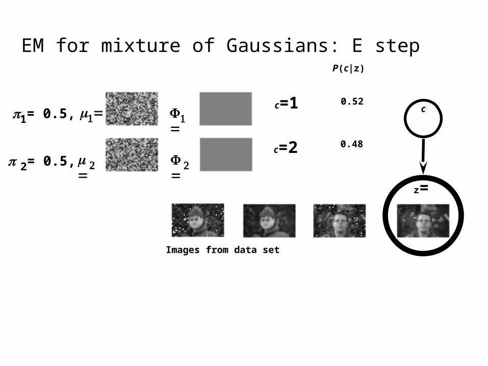
c=1
Images from data set
z=
c=2
P(c|z)
c0.52
0.48
1= 0.5,
2= 0.5,
EM for mixture of Gaussians: E step

Images from data set
z=
cc=1
c=2
P(c|z)
0.51
0.49
1= 0.5,
2= 0.5,
EM for mixture of Gaussians: E step

Images from data set
z=
cc=1
c=2
P(c|z)
0.48
0.52
1= 0.5,
2= 0.5,
EM for mixture of Gaussians: E step

Images from data set
z=
cc=1
c=2
P(c|z)
0.43
0.57
1= 0.5,
2= 0.5,
EM for mixture of Gaussians: E step

c
1= 0.5,
2= 0.5,
z
Set 1 to the average of zP(c=1|z)
Set 2 to the average of zP(c=2|z)
EM for mixture of Gaussians: M step

c
1= 0.5,
2= 0.5,
z
Set 1 to the average of zP(c=1|z)
Set 2 to the average of zP(c=2|z)
EM for mixture of Gaussians: M step
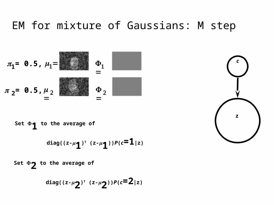
c
1= 0.5,
2= 0.5,
z
Set 1 to the average of
diag((z-1)T (z-1))P(c=1|z)
Set 2 to the average of
diag((z-2)T (z-2))P(c=2|z)
EM for mixture of Gaussians: M step

c
1= 0.5,
2= 0.5,
z
Set 1 to the average of
diag((z-1)T (z-1))P(c=1|z)
Set 2 to the average of
diag((z-2)T (z-2))P(c=2|z)
EM for mixture of Gaussians: M step

… after iterating to convergence:
c
z
1= 0.6,
2= 0.4,
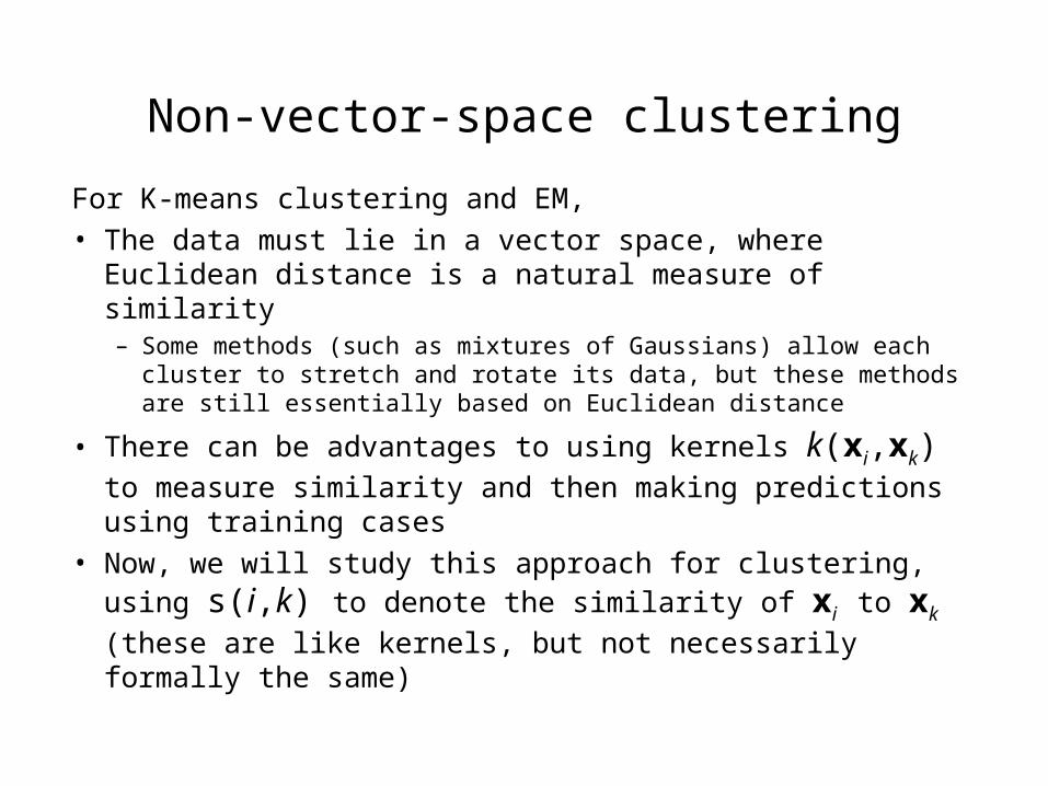
Non-vector-space clustering
For K-means clustering and EM,• The data must lie in a vector space, where Euclidean
distance is a natural measure of similarity– Some methods (such as mixtures of Gaussians) allow each
cluster to stretch and rotate its data, but these methods are still essentially based on Euclidean distance
• There can be advantages to using kernels k(xi,xk) to
measure similarity and then making predictions using training cases
• Now, we will study this approach for clustering, using s(i,k) to denote the similarity of xi to xk (these are like
kernels, but not necessarily formally the same)

K-centers clustering(aka K-medoids clustering and K-medians clustering)

Randomly chooseinitial exemplars,(data centers)
K-centers clustering(aka K-medoids clustering and K-medians clustering)

Assign data points tonearest centers
K-centers clustering(aka K-medoids clustering and K-medians clustering)

For each cluster,pick best newcenter
K-centers clustering(aka K-medoids clustering and K-medians clustering)

K-centers clustering(aka K-medoids clustering and K-medians clustering)
For each cluster,pick best newcenter

K-centers clustering(aka K-medoids clustering and K-medians clustering)
Assign data points tonearest centers
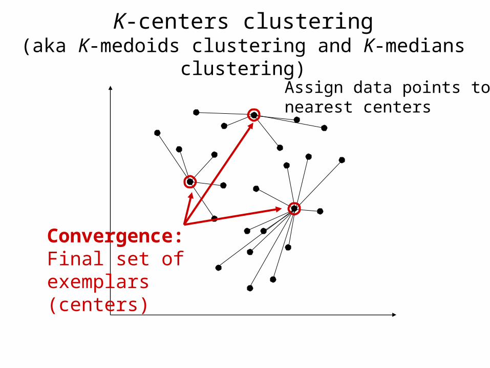
Assign data points tonearest centers
K-centers clustering(aka K-medoids clustering and K-medians clustering)
Convergence:Final set ofexemplars(centers)

The K-centers clustering algorithm
• Denote the index of the center that xi is currently
assigned to by ci (ci i indicates that xi is a center)
• Initialization: Randomly pick K points and set ck = k
• Loop until convergence
– For all i s.t. ci i set ci argmaxk:ck=k s(i,k)
– For all k s.t. ck k
• Compute k new argmaxi:ci=k (j:cj=k s(j,i))
• For all i s.t. ci k set ci k new
• This is similar to K-means clustering, except that the means are always data points

Handwritten digit clustering and recognition

Example: Clustering 3000 Buffalo digits
Similarity: s(i,k) = - || xi - xk ||2
K=10
K=20
K=40
K=80

The effect of random initialization
Squared error
Affinity propagation

k-centers clusteringHow good is the solution?
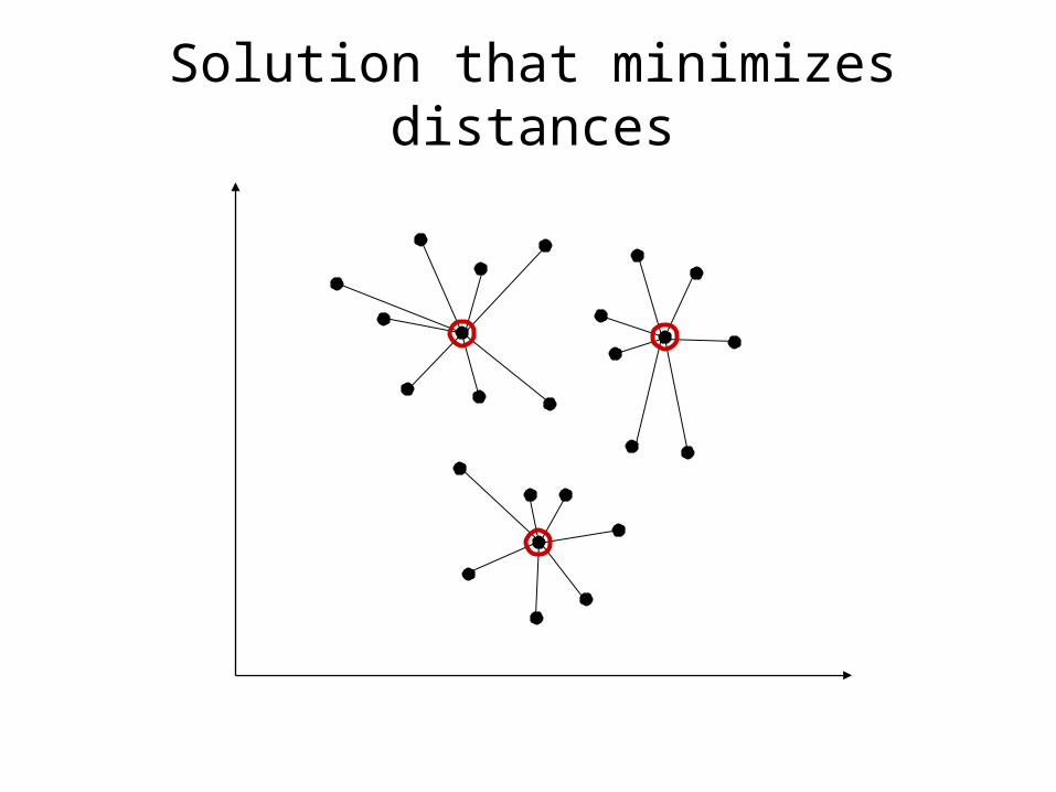
Solution that minimizes distances

ITERATION # 0
-5 0 +5-5
0
+5
ITERATION # 1
-5 0 +5-5
0
+5
non-exemplar exemplar
Affinity propagation(Frey & Dueck, Science, Feb 2007)
ITERATION # 1
-5 0 +5-5
0
+5
non-exemplar exemplar
ITERATION # 2
-5 0 +5-5
0
+5
non-exemplar exemplar
ITERATION # 3
-5 0 +5-5
0
+5
non-exemplar exemplar
ITERATION # 4
-5 0 +5-5
0
+5
non-exemplar exemplar
ITERATION # 5
-5 0 +5-5
0
+5
non-exemplar exemplar
ITERATION # 6
-5 0 +5-5
0
+5
non-exemplar exemplar
ITERATION # 7
-5 0 +5-5
0
+5
non-exemplar exemplar
ITERATION # 8
-5 0 +5-5
0
+5
non-exemplar exemplar
ITERATION # 9
-5 0 +5-5
0
+5
non-exemplar exemplar
ITERATION #10
-5 0 +5-5
0
+5
non-exemplar exemplar
ITERATION #11
-5 0 +5-5
0
+5
non-exemplar exemplar
ITERATION #12
-5 0 +5-5
0
+5
non-exemplar exemplar
ITERATION #13
-5 0 +5-5
0
+5
non-exemplar exemplar
ITERATION #14
-5 0 +5-5
0
+5
non-exemplar exemplar
ITERATION #15
-5 0 +5-5
0
+5
non-exemplar exemplar
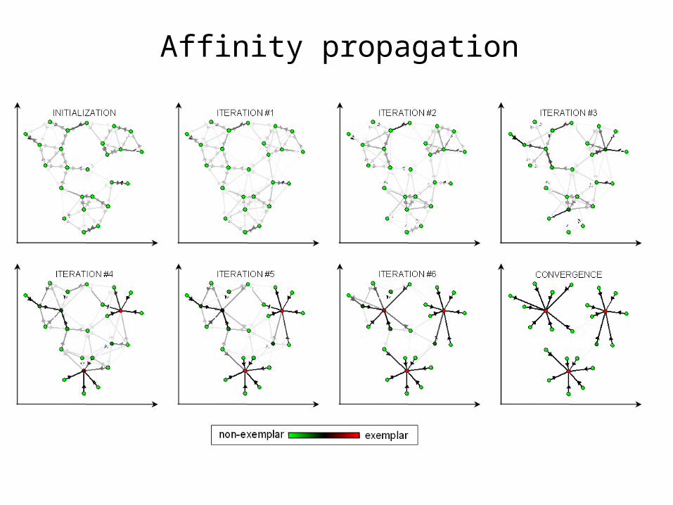
Affinity propagation

ITERATION #15
-5 0 +5-5
0
+5
non-exemplar exemplar
Affinity propagation

Solution that minimizes distances
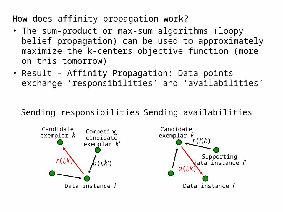
How does affinity propagation work?• The sum-product or max-sum algorithms (loopy belief
propagation) can be used to approximately maximize the k-centers objective function (more on this tomorrow)
• Result – Affinity Propagation: Data points exchange ‘responsibilities’ and ‘availabilities’
Sending responsibilities
Candidateexemplar k
r(i,k)
Data instance i
Competingcandidate
exemplar k’
a(i,k’)
Sending availabilities
Candidateexemplar k
a(i,k)
Data instance i
Supportingdata instance i’
r(i’,k)

Sending responsibilitiesCandidateexemplar k
r(i,k)
Data instance i
Competingcandidate
exemplar k’
a(i,k’)
Sending availabilitiesCandidateexemplar k
a(i,k)
Data instance i
Supportingdata instance i’
r(i’,k)
Making decisions:
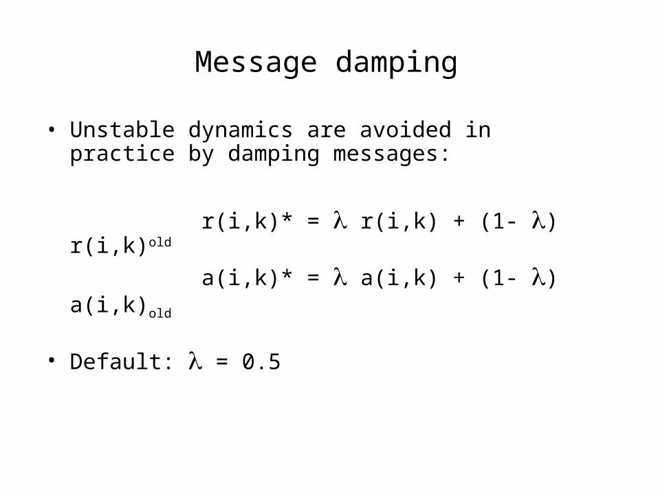
Message damping
• Unstable dynamics are avoided in practice by damping messages:
r(i,k)* = r(i,k) + (1- ) r(i,k)old
a(i,k)* = a(i,k) + (1- ) a(i,k)old
• Default: = 0.5

MATLAB implementation(from http://www.psi.toronto.edu/affinitypropagation)

Document summarization using affinity propagation
s(sentence i,sentence k) = - Number of bits needed to encode the words in sentence i using the words in sentence k and a global dictionary
Preference(sentence k) = - Number of bits needed to encode the words in sentence k using only the global dictionary
1) Affinity propagation identifies exemplars by recursively sending real-valued messages between pairs of data points.
2) The number of identified exemplars (number of clusters) is influenced by the values of the input preferences, but also emerges from the message-passing procedure.
3) The availability is set to the self-responsibility plus the sum of the positive responsibilities the candidate exemplar receives from other points.
4) For different numbers of clusters, the reconstruction errors achieved by affinity propagation and k-centers clustering are compared.

Questions?

How are we doing on the pass sequence?
Can clustering be used to automatically learn the two
modes of tracking for the man in the white shirt?
• Maybe, but this system is getting too complex!• Is there any simple way to put the pieces
together…?