Clustered Binary Logistic Regression in Teratology Data Presentation...Clustered Binary Logistic...

Clustered Binary Logistic Regression in Teratology Data

Jorge G. Morel, Ph.D. Adjunct Professor

University of Maryland Baltimore County

Division of Biostatistics and Epidemiology Cincinnati Children’s Hospital Medical Center.

September 9, 2014

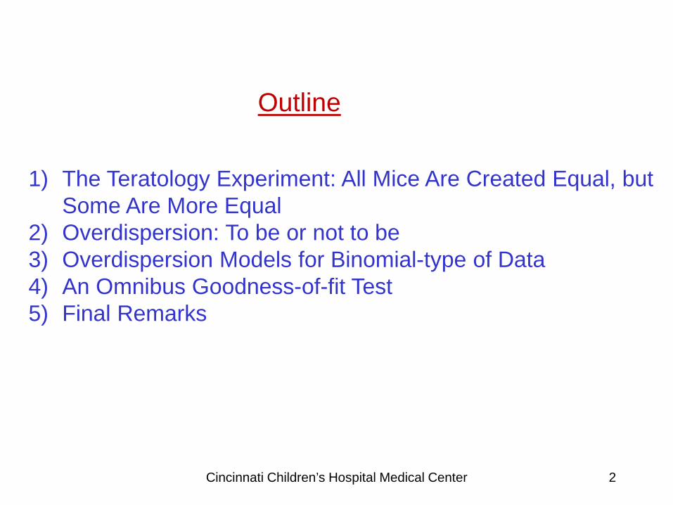
1) The Teratology Experiment: All Mice Are Created Equal, but Some Are More Equal

2) Overdispersion: To be or not to be 3) Overdispersion Models for Binomial-type of Data 4) An Omnibus Goodness-of-fit Test 5) Final Remarks

Outline

Cincinnati Children’s Hospital Medical Center 2

All Mice Are Created Equal, but Some Are More Equal


Two-way factorial design with n=81 pregnant C57BL/6J mice

• Purpose: to investigate synergistic effect of the

anticonvulsant phenytoin (PHT) and thrichloropropane oxide (TCPO) on the prenatal development of inbred mice

• Presence or absence of ossification at the phalanges at

both the left and right forepaws is considered a measure of teratogenic effect

• Outcome: presence or absence of ossification at the

phalanges. For simplicity we analyze outcome on the left middle third phalanx


Hartsfield et al. (1990), Morel and Neerchal (1997), PROC FMM Documentation


Ossification Data* Group Observations Control 8/8, 9/9, 7/9, 0/5, 3/3, 5/8, 9/10, 5/8, 5/8, 1/6, 0/5, 8/8, 9/10, 5/5, 4/7, 9/10, 6/6, 3/5 Sham 8/9, 7/10, 10/10, 1/6, 6/6, 1/9, 8/9, 6/7, 5/5, 7/9, 2/5, 5/6, 2/8, 1/8, 0/2, 7/8, 5/7 PHT 1/9, 4/9, 3/7, 4/7, 0/7, 0/4, 1/8, 1/7, 2/7, 2/8, 1/7, 0/2, 3/10, 3/7, 2/7, 0/8, 0/8, 1/10, 1/1 TCPO 0/5, 7/10, 4/4, 8/11, 6/10, 6/9, 3/4, 2/8, 0/6, 0/9, 3/6, 2/9, 7/9, 1/10, 8/8, 6/9 PHT+TCPO 2/2, 0/7, 1/8, 7/8, 0/10, 0/4, 0/6, 0/7, 6/6, 1/6, 1/7

*Number of fetuses showing ossification / litter size. PHT: phenytoin; TCPO: trichloropropene oxide.

• Presence or absence of ossification at the phalanges at both the left and right forepaws is considered a measure of teratogenic effect

• The experiment thus can be seen as a 2 x 2 factorial, with PHT and

TCPO as the two factors • The levels of PHT are 60 mg/kg and 0 mg/kg, and the levels of TCPO

are 100 mg/kg and 0 mg/kg.



Ossification Data* Group Observations PHT+TCPO 2/2, 0/7, 1/8, 7/8, 0/10, 0/4, 0/6, 0/7, 6/6, 1/6, 1/7


( )

( ) ( )

( )

11

jj 1

11

jj 1

j j

11

jj 1

2j j

j

tˆ 0.2535

m

If t 's were distributed as Binomial random variables with parameters , m

ˆ ˆ1ˆ ˆVar 0.0027m

ˆA consistent estimator of variance of is

ˆn (t m )ˆ Var

=

=

=

π = =

π

π − ππ = =

π

− ππ =

∑

∑

∑

n

12

n

jj 1

0.0142

m (n 1)

=

=

=

−

∑

∑Cincinnati Children’s Hospital Medical Center 6

• Overdispersion is also known as Extra Variation • Arises when Binary/Count data exhibit variances larger

than those permitted by the Binomial/Poisson model • Usually caused by clustering or a lack of independence • It might be also caused by a model misspecification

“In fact, some would maintain that over-dispersion is the norm in practice and nominal dispersion the exception.”

McCullagh and Nelder (1989, Pages 124-125)

Overdispersion: To be or not to be.


• Some Distributions to Model Binomial Data with Overdispersion: o Beta-binomial o Random-clumped Binomial o Zero-inflated Binomial o Generalized Binomial

• Some Distributions to Model Count Data with Overdispersion:

o Negative-binomial o Zero-inflated Poisson o Zero-inflated Negative-binomial o Hurdle Poisson o Hurdle Negative-binomial o Generalized Poisson



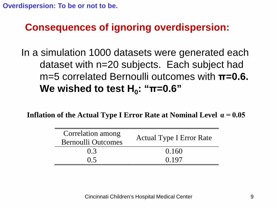
Consequences of ignoring overdispersion:

In a simulation 1000 datasets were generated each dataset with n=20 subjects. Each subject had m=5 correlated Bernoulli outcomes with π=0.6. We wished to test H0: “π=0.6”

Inflation of the Actual Type I Error Rate at Nominal Level α = 0.05

Correlation among

Bernoulli Outcomes Actual Type I Error Rate

0.3 0.160 0.5 0.197



Consequences of ignoring overdispersion: • Standard errors of Naïve estimates are smaller

than they should be. • This results in inflated Type I Error Rates, i.e.,

False Positive Rates are larger than nominal ones.

• Furthermore, coverage probabilities of confidence intervals are lower than nominal levels.

• Erroneous inferences !!!



Overdispersion Models for Binomial-type of Data: The Beta-binomial Distribution Skellam (1948)

These babies use about m=20 diapers (changes) per week. Let us count the number of diapers leaking (T)

P1 P2 P3

P4

P5 P7

The Beta-binomial assumes different probabilities of leakage for different babies, drawn from a Beta distribution.


( )( )

( ) ( )

( )( )

( ) { }( )

2 2

Thus T | P ~ Binomial P;m

It is further assumed P 's are i.i.d. ~ Beta a,b

a C , b C 1 , C 1

Then the unconditional distribution of T is Beta-binomial

m C t C m t C(1 )Pr(T t)

t m C C C 1

= π = − π = −ρ ρ

Γ Γ + π Γ − + − π = = Γ + Γ π Γ − ( ){ } ,

t 0,1,...,m

π

=

Overdispersion Models for Binomial-type of Data: The Beta-binomial Distribution


( )( )

( ) ( )

( )

m

m

i

i i i i

Let Y,Y ,...,Y be i.i.d. Bernoulli

Let U ,...., U be i.i.d. Uniform ,For each i, i ,...,m, define Y as

Y Y I U Y I U

where I . is an indicator funct

π

=

= ≤ ρ + > ρ

0 01

1

0

0 1 1

m

ii

ion andThen, define T as

T Y=

≤ ρ ≤

=∑1

0 1

(Morel and Nagaraj, 1993; Morel and Neerchal, 1997; Neerchal and Morel, 1998) Results from an effort to model meaningfully the physical mechanism behind the extra variation

Overdispersion Models for Binomial-type of Data: The Random-clumped Binomial Distribution (aka Binomial Cluster in PROC FMM)


( )

( )( )( )

π

−

+

ρ

π

=

It can be shown: ,

where Y ~ Bernoulli

N ~ Binomial ; m , Y and N independent

X | N ~ Bin

T YN X |N

omial ; m N if N < m

• The outcome given by Y is duplicated a random number of times N, N = 0,1,…,m. This is represented by YN.

• The remaining m - N units within the cluster provide independent

Bernoulli responses. This is represented by (X|N)

Overdispersion Models for Binomial-type of Data: The Random-clumped Binomial Distribution


1 1

1 1

?

?

?

N m−N

YN X given N (a)

0 0

0 0

?

?

?

N m−N

YN X given N (b)

YN might characterize the influence of a “leader” in a stop-smoking or a stop-drinking program, or a genetic trait which is passed on with a certain probability to offspring of the

same mother



( ) ( ) ( ) ( )

( ){ }( ){ }

= = π = + − π =

=

− ρ π + ρ

− ρ π

1 2

1

2

Pr ob T t Pr X t 1 Pr X t , t 0,1,...,m,

X ~ Binomial 1 ; m ,

X ~ Binomial 1 ; m



( )

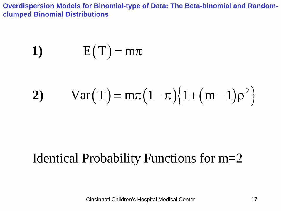
( ) ( ) ( ){ }2

E T m

Var T m 1 1 m 1

Identical Probability Functions for m=2

= π

= π − π + − ρ

1)

2)

Overdispersion Models for Binomial-type of Data: The Beta-binomial and Random-clumped Binomial Distributions


Beta-binomial and Binomial


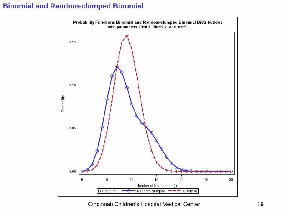
Binomial and Random-clumped Binomial


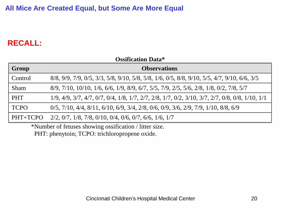
Ossification Data* Group Observations Control 8/8, 9/9, 7/9, 0/5, 3/3, 5/8, 9/10, 5/8, 5/8, 1/6, 0/5, 8/8, 9/10, 5/5, 4/7, 9/10, 6/6, 3/5 Sham 8/9, 7/10, 10/10, 1/6, 6/6, 1/9, 8/9, 6/7, 5/5, 7/9, 2/5, 5/6, 2/8, 1/8, 0/2, 7/8, 5/7 PHT 1/9, 4/9, 3/7, 4/7, 0/7, 0/4, 1/8, 1/7, 2/7, 2/8, 1/7, 0/2, 3/10, 3/7, 2/7, 0/8, 0/8, 1/10, 1/1 TCPO 0/5, 7/10, 4/4, 8/11, 6/10, 6/9, 3/4, 2/8, 0/6, 0/9, 3/6, 2/9, 7/9, 1/10, 8/8, 6/9 PHT+TCPO 2/2, 0/7, 1/8, 7/8, 0/10, 0/4, 0/6, 0/7, 6/6, 1/6, 1/7

*Number of fetuses showing ossification / litter size. PHT: phenytoin; TCPO: trichloropropene oxide.

RECALL:



( )j j j j j j

j j

j

Let TCPO ,PHT ,TCPO *PHT be the probability of ossification

j 1,2,...,811 if TCPO is present 1 if PHT is present

TCPO PHT 0 if TCPO is absent 0 if PHT is absent

Let T denote the tota

π ≡ π

=

= =

( )( )

j

j j j

j j j

j

l number of fetuses for which ossification of

the left middle third phalanx occurred out of a litter containing m fetuses.

T ~ Binomial ;m

T ~ Beta-binomial , ;m

T ~ Random-clumped

π

π ρ

( )

j0 1 j 2 j 3

j

jj

j

j 0ln *TCPO *PHT *TCPO *PHT 1

, ;m

ln1 π = β

ρ= α −ρ

+β +β +

π ρ

β − π

Link functions :



data ossi; length tx $8; input tx$ n @@; do i=1 to n; input t m @@; output; end; drop n i; datalines; Control 18 8 8 9 9 7 9 0 5 3 3 5 8 9 10 5 8 5 8 1 6 0 5 8 8 9 10 5 5 4 7 9 10 6 6 3 5 Control 17 8 9 7 10 10 10 1 6 6 6 1 9 8 9 6 7 5 5 7 9 2 5 5 6 2 8 1 8 0 2 7 8 5 7 PHT 19 1 9 4 9 3 7 4 7 0 7 0 4 1 8 1 7 2 7 2 8 1 7 0 2 3 10 3 7 2 7 0 8 0 8 1 10 1 1 TCPO 16 0 5 7 10 4 4 8 11 6 10 6 9 3 4 2 8 0 6 0 9 3 6 2 9 7 9 1 10 8 8 6 9 PHT+TCPO 11 2 2 0 7 1 8 7 8 0 10 0 4 0 6 0 7 6 6 1 6 1 7 ; data ossi; set ossi; array xx{3} x1-x3; do i=1 to 3; xx{i}=0; end; pht = 0; tcpo = 0; if (tx='TCPO') then do; xx{1} = 1; tcpo = 100; end; else if (tx='PHT') then do; xx{2} = 1; pht = 60; end; else if (tx='PHT+TCPO') then do; pht = 60; tcpo = 100; xx{1} = 1; xx{2} = 1; xx{3}=1; end; run;



title "Fitting a Beta-binomial in PROC NLMIXED"; proc nlmixed data=ossification; parms b0=0, b1=0, b2=0, b3=0, a0=0; linr = a0; rho = 1/(1+exp(-linr)); c = 1 / rho / rho - 1; if (tx='Control') then linp = b0; else if (tx='TCPO') then linp = b0+b1; else if (tx='PHT') then linp = b0+b2; else if (tx='PHT+TCPO') then linp = b0+b1+b2+b3; pi = 1/(1+exp(-linp)); pic = 1 - pi; z = lgamma(m+1) - lgamma(t+1) - lgamma(m_t+1); ll = z + lgamma(c) + lgamma(t+c*pi) + lgamma(m_t+c*pic) - lgamma(m+c) - lgamma(c*pi) - lgamma(c*pic); model t ~ general(ll); estimate 'Pi Control' 1/(1+exp(-b0)); estimate 'Pi TCPO' 1/(1+exp(-b0-b1)); estimate 'Pi PHT' 1/(1+exp(-b0-b2)); estimate 'Pi PHT+TCPO' 1/(1+exp(-b0-b1-b2-b3)); estimate 'Logarithm Odds-Ratio PHT when TCPO Absent ' b2; estimate 'Logarithm Odds-Ratio PHT when TCPO Present' b2+b3; estimate 'Common Rho*Rho' 1/(1+exp(-a0))/(1+exp(-a0)); run; title;



Additional Estimates

Label Estimate Standard Error

DF t Value Pr > |t| Alpha Lower Upper

Pi Control 0.6546 0.05124 81 12.77 <.0001 0.05 0.5526 0.7565

Pi TCPO 0.4240 0.07372 81 5.75 <.0001 0.05 0.2773 0.5707

Pi PHT 0.2911 0.06336 81 4.59 <.0001 0.05 0.1650 0.4172

Pi PHT+TCPO 0.2280 0.08255 81 2.76 0.0071 0.05 0.06378 0.3923

Logarithm Odds-Ratio PHT when TCPO Absent

-1.5291 0.3956 81 -3.87 0.0002 0.05 -2.3161 -0.7421

Logarithm Odds-Ratio PHT when TCPO Present

-0.9129 0.5608 81 -1.63 0.1075 0.05 -2.0288 0.2030

Common Rho*Rho 0.3400 0.04860 81 7.00 <.0001 0.05 0.2433 0.4367



title "Fitting a Beta-binomial in PROC FMM"; proc fmm data=ossi; model t/m = x1-x3 / dist=betabinomial; run; proc fmm data=ossi; class tcpo pht; model t/m = tcpo pht tcpo*pht / dist=betabinomial; run;



Fitting a Beta-binomial in PROC FMM

The FMM Procedure Model Information

Data Set WORK.OSSI

Response Variable (Events) t

Response Variable (Trials) m

Type of Model Homogeneous Regression Mixture

Distribution Beta-Binomial

Components 1

Link Function Logit

Estimation Method Maximum Likelihood

Fit Statistics

-2 Log Likelihood 306.6

AIC (smaller is better) 316.6

AICC (smaller is better) 317.4

BIC (smaller is better) 328.5

Pearson Statistic 87.5379

Parameter Estimates for 'Beta-Binomial' Model

Effect Estimate Standard Error z Value Pr > |z|

Intercept 0.7043 0.2341 3.01 0.0026

x1 -0.7822 0.4017 -1.95 0.0515

x2 -1.6917 0.4018 -4.21 <.0001

x3 0.6770 0.6902 0.98 0.3267

Scale Parameter 1.9642 0.4758



title "Fitting a Random-clumped Binomial in PROC FMM"; proc fmm data=ossi; model t/m = / dist=binomcluster; probmodel x1-x3; run; proc fmm data=ossi; class tcpo pht; model t/m = / dist=binomcluster; probmodel tcpo pht tcpo*pht; run;

WARNING: Note that the MODEL statement specifies a model for the overdispersion parameter, not the link for the mean.



Fitting a Random-clumped Binomial in PROC FMM

The FMM Procedure Model Information

Data Set WORK.OSSI

Response Variable (Events) t

Response Variable (Trials) m

Type of Model Binomial Cluster

Distribution Binomial Cluster

Components 2

Link Function Logit

Estimation Method Maximum Likelihood

Fit Statistics

-2 Log Likelihood 305.1

AIC (smaller is better) 315.1

AICC (smaller is better) 315.9

BIC (smaller is better) 327.0

Pearson Statistic 89.2077

Effective Parameters 5

Effective Components 2

Parameter Estimates for 'Binomial Cluster' Model

Component Effect Estimate Standard

Error z Value Pr > |z|

Inverse Linked

Estimate

1 Intercept 0.3356 0.1714 1.96 0.0503 0.5831

Parameter Estimates for Mixing Probabilities

Effect Estimate Standard Error z Value Pr > |z|

Intercept 0.6392 0.2266 2.82 0.0048

x1 -0.9457 0.3711 -2.55 0.0108

x2 -1.5291 0.3956 -3.87 0.0001

x3 0.6162 0.6678 0.92 0.3561



Ossification Example with the OverdispersionModelsInR package

> ossification <- read.table("ossification.dat", header = TRUE) > tail(ossification) litter group oss size 76 76 PHT+TCPO 0 4 77 77 PHT+TCPO 0 6 78 78 PHT+TCPO 0 7 79 79 PHT+TCPO 6 6 80 80 PHT+TCPO 1 6 81 81 PHT+TCPO 1 7 > levels(ossification$group) [1] "Control" "PHT" "PHT+TCPO" "TCPO"

Consider two models: • RCB: 𝑇𝑇𝑖𝑖 ∼ 𝑅𝑅𝑅𝑅𝑅𝑅(𝑚𝑚𝑖𝑖 ,𝜋𝜋𝑖𝑖 ,𝜌𝜌) • BB: 𝑇𝑇𝑖𝑖 ∼ 𝑅𝑅𝑅𝑅 𝑚𝑚𝑖𝑖 ,𝜋𝜋𝑖𝑖 ,𝜌𝜌 Both models have a common regression on 𝜋𝜋𝑖𝑖 given by • 𝑔𝑔 𝜋𝜋𝑖𝑖 = 𝛽𝛽0 + 𝛽𝛽1TCPO𝑖𝑖 + 𝛽𝛽2PHT𝑖𝑖 + 𝛽𝛽3 TCPO𝑖𝑖 ⋅ PHT𝑖𝑖

Read the data.

Courtesy of Dr. Andrew Raim, Census Bureau


tcpo <- ossification$group %in% c("TCPO", "PHT+TCPO") pht <- ossification$group %in% c("PHT", "PHT+TCPO") both <- ossification$group %in% c("PHT+TCPO") X <- cbind(1, tcpo, pht, both) colnames(X) <- c("Intercept", "TCPO", "PHT", "PHT+TCPO") y <- ossification$oss m <- ossification$size

var.names <- c(colnames(X), "rho", "Pi Control", "Pi PHT", "Pi TCPO", "Pi PHT+TCPO", "Log-odds-ratio PHT vs. Control, TCPO Present", "Log-odds-ratio PHT vs. Control, TCPO Absent", "rho.sq") extra.tx <- function(theta){ list(Pi.control = plogis(theta$Beta[1]), Pi.TCPO = plogis(sum(theta$Beta[1:2])), Pi.PHT = plogis(sum(theta$Beta[c(1,3)])), Pi.PHT_TCPO = plogis(sum(theta$Beta[1:4])), log.odds.tcpo = theta$Beta[3], log.odds.notcpo = sum(theta$Beta[3:4]), rho.sq = theta$rho^2) } fit.rcb.x.out <- fit.rcb.x.mle(y, m, X, extra.tx = extra.tx, var.names = var.names) fit.bb.x.out <- fit.bb.x.mle(y, m, X, extra.tx = extra.tx, var.names = var.names)

Prepare the data for model fitting.

Fit the models, specifying “extra” estimates (quantities not required to evaluate the likelihood).




> fit.bb.x.out Fit for model: y[i] ~indep~ BB(m[i], Pi[i], rho) logit(Pi[i]) = x[i]^T Beta --- Parameter Estimates --- Estimate SE t-val P(|t|>t-val) Gradient Intercept 0.7043 0.2341 3.0087 0.0035 -0.0002 TCPO -0.7822 0.4017 -1.9474 0.0550 -0.0001 PHT -1.6917 0.4018 -4.2102 6.563E-05 -0.0001 PHT+TCPO 0.6769 0.6902 0.9808 0.3296 3.822E-05 rho 0.5808 0.0466 12.4609 0.000E+00 -3.082E-05 --- Additional Estimates --- Estimate SE t-val P(|t|>t-val) Gradient Pi Control 0.6691 0.0518 12.9117 0.000E+00 -3.410E-05 Pi PHT 0.4805 0.0816 5.8870 8.548E-08 -7.051E-05 Pi TCPO 0.2714 0.0628 4.3211 4.376E-05 -5.811E-05 Pi PHT+TCPO 0.2511 0.0883 2.8434 0.0056 -7.222E-05 Log-OR PHT vs. Control, w/TCPO -1.6917 0.4018 -4.2102 6.563E-05 -0.0001 Log-OR PHT vs. Control, w/o TCPO -1.0148 0.5727 -1.7720 0.0802 -0.0001 rho.sq 0.3374 0.0541 6.2304 1.969E-08 -3.580E-05 -- Degrees of freedom = 81 LogLik = -153.2876 AIC = 316.5751 AICC = 317.3751 BIC = 328.5474

BB Results:


> fit.rcb.x.out Fit for model: y[i] ~indep~ RCB(m[i], Pi[i], rho) logit(Pi[i]) = x[i]^T Beta --- Parameter Estimates --- Estimate SE t-val P(|t|>t-val) Gradient Intercept 0.6392 0.2266 2.8204 0.0060 0.0003 TCPO -0.9456 0.3711 -2.5481 0.0127 5.367E-05 PHT -1.5291 0.3956 -3.8657 0.0002 4.795E-05 PHT+TCPO 0.6161 0.6678 0.9226 0.3589 0.0001 rho 0.5831 0.0417 13.9926 0.000E+00 -4.272E-05 --- Additional Estimates --- Estimate SE t-val P(|t|>t-val) Gradient Pi Control 0.6546 0.0512 12.7741 0.000E+00 5.989E-05 Pi PHT 0.4240 0.0737 5.7510 1.517E-07 7.779E-05 Pi TCPO 0.2911 0.0634 4.5946 1.573E-05 6.456E-05 Pi PHT+TCPO 0.2280 0.0826 2.7623 0.0071 9.019E-05 Log-OR PHT vs. Control, w/TCPO -1.5291 0.3956 -3.8657 0.0002 4.795E-05 Log-OR PHT vs. Control, w/o TCPO -0.9129 0.5608 -1.6278 0.1074 0.0002 rho.sq 0.3400 0.0486 6.9963 6.856E-10 -4.982E-05 -- Degrees of freedom = 81 LogLik = -152.5267 AIC = 315.0534 AICC = 315.8534 BIC = 327.0257


RCB Results:


Beta Estimates and Standard Errors of the Ossification Data

Distribution

Binomial Beta-binomial Random-clumped Binomial

Parameter Estimate Standard Error Estimate Standard

Error Estimate Standard Error

Intercept ( )0β̂ 0.8323 0.1365 0.7043 0.2341 0.6392 0.2266

TCPO ( )1β̂ -0.8481 0.2239 -0.7822 0.4017 -0.9457 0.3711

PHT ( )2β̂ -2.1094 0.2505 -1.6917 0.4018 -1.5291 0.3956

TCPO + PHT ( )3β̂ 1.0453 0.4107 0.6770 0.6902 0.6162 0.6678

Overdispersion (ρ2 ) -- -- 0.3374 0.05415 0.3400 0.04860

- 2 * Log Likelihood 401.8 -- 306.6 -- 305.1 -- PHT: phenytoin; TCPO: trichloropropene oxide

Akaike Information Criteria (AIC) practically the same for BC and RCB



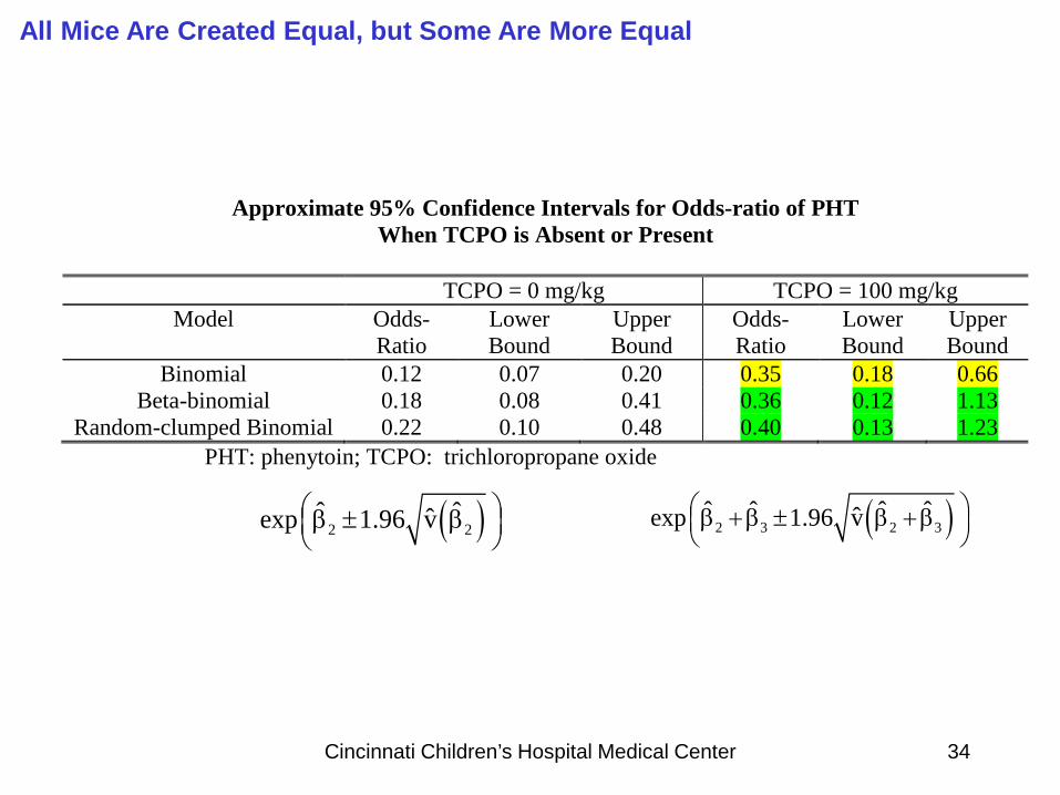
Approximate 95% Confidence Intervals for Odds-ratio of PHT When TCPO is Absent or Present

TCPO = 0 mg/kg TCPO = 100 mg/kg

Model Odds-Ratio

Lower Bound

Upper Bound

Odds-Ratio

Lower Bound

Upper Bound

Binomial 0.12 0.07 0.20 0.35 0.18 0.66 Beta-binomial 0.18 0.08 0.41 0.36 0.12 1.13

Random-clumped Binomial 0.22 0.10 0.48 0.40 0.13 1.23 PHT: phenytoin; TCPO: trichloropropane oxide



( )2 2ˆ ˆˆexp 1.96 v β ± β

( )2 3 2 3

ˆ ˆ ˆ ˆˆexp 1.96 v β +β ± β +β

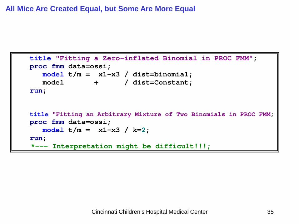
title "Fitting a Zero-inflated Binomial in PROC FMM"; proc fmm data=ossi; model t/m = x1-x3 / dist=binomial; model + / dist=Constant; run; title "Fitting an Arbitrary Mixture of Two Binomials in PROC FMM; proc fmm data=ossi; model t/m = x1-x3 / k=2; run; *--- Interpretation might be difficult!!!;



Parameter Estimates for 'Binomial' Model

Component Effect Estimate Standard Error z Value Pr > |z|

1 Intercept 1.6876 0.2049 8.23 <.0001

1 x1 -0.7364 0.3324 -2.22 0.0267

1 x2 -2.5593 0.3644 -7.02 <.0001

1 x3 4.3154 1.1270 3.83 0.0001

2 Intercept -1.6757 0.4668 -3.59 0.0003

2 x1 -0.4363 0.6838 -0.64 0.5234

2 x2 -0.6293 0.9055 -0.70 0.4870

2 x3 -0.1100 1.1947 -0.09 0.9267

Parameter Estimates for Mixing Probabilities

Effect

Linked Scale

Probability Estimate Standard Error z Value Pr > |z|

Intercept 0.5289 0.2690 1.97 0.0493 0.6292



• Omnibus tests are designed to test if a specific distribution fits the data well. The null hypothesis is that the data come from a population with a specific distribution, while the alternative hypothesis states that the data do not come from that distribution.

• Since there is no model specified in the alternative hypothesis, we

cannot obtain maximum likelihood estimates under the alternative. • The Shapiro-Wilk test of normality is an example of an omnibus test.

• When the mj’s are different, the construction of a Pearson’s

Goodness-of-fit statistic is not straightforward because the observed and expected frequencies are not associated with a unique value of m

Omnibus Goodness-of-fit Test


• Neerchal and Morel (1998) proposed an extension of the traditional Pearson’s Chi-square statistic

when the clusters sizes are allowed to be different and/or covariates are present in the model

• Asymptotic properties of this test have been investigated by

Sutradhar et al. (2008).

• Test can be applied to Binomial, Beta-binomial, Random-clumped Binomial (aka Binomial Cluster), Zero-inflated Binomial, Distributions

( )c

22s s s

s 1X O E E

=

= −∑



[ )[ )[ ) [ )[ ]

=

=

=

j

j

j ths

j

j ths

j

tCompute for j 1,2,...,n

m

Then get t

O : Observed number of 's in the s int erval, s 1,2,...,cm

tE : Expected number of 's in the s int erval, s 1,2,...,c

m

A1 A2 A3 Ac-1 Ac

Divide the [0,1] interval into C mutually exclusive intervals:

0 1



2df

Properties of GOF:

1) GOF X

2) Degrees of freedom (df) of GOF is between: C 1 (Number of Parameters Estimated in the Model) and C 1 (see chapter 30 of Kendall, Stuart, and Ord, 19

− − −

91)

3) Underlying DF and P-value can be obtained via Parametric Bootstrapping

4) GOF is also applicable when cluster sizes are not the same and/or covariates are present



Results Omnibus Goodness-of-fit Tests

Distribution GOF-Stat Degrees of Freedom P-Value

Binomial 56.94 Lower Bound 4 < 0.01 Upper Bound 8 < 0.01

Beta-binomial 9.79 Lower Bound 3 0.02 Upper Bound 8 0.28

Binomial Cluster 6.81 Lower Bound 3 0.08 Upper Bound 8 0.56



Parametric Bootstrapping Results

Based on 5,000 Replications

Distribution Parameter Estimate

Beta-binomial Degrees of Freedom 5.83

P-value 0.11

Random-clumped Binomial Degrees of Freedom 5.79

P-value 0.31



Conclusions: a) Both distributions fit the data, however, the RCB seems to

provide a better fit than the BB b) Since in this example the RCB provides a clear mechanism on

how the offspring inherit the genetic trait, I prefer the RCB over the BB



Final Remarks

“over-dispersion is the norm in practice and nominal dispersion the exception”

Beta-binomial and Binomial Cluster are now available in SAS® PROC FMM and in R

An Omnibus Goodness-of-test is available. See Morel and Neerchal (2012) “Overdispersion Models in SAS®”

Beta-binomial and Random-clumped are just the tip of the iceberg. They belong to the Generalized Linear Overdispersion Models (GLOM)


Binomial Distribution

Beta-binomial

1) Binomial Distribution

Random-clumped Binomial

Zero-inflated Binomial

Poisson Distribution

Negative-binomial

Zero-inflated Negative-binomial

Zero-inflated Poisson

Hurdle Models

2) Poisson Distribution

Multinomial Distribution

3) Multinomial Distribution

Dirichlet-multinomial

Random-clumped Multinomial

Generalized Poisson

Generalized Binomial

Final Remarks


Thanks for your attention!


Clustered Binary Logistic Regression in Teratology Data Presentation...Clustered Binary Logistic...

Documents

Transcript of Clustered Binary Logistic Regression in Teratology Data Presentation...Clustered Binary Logistic...