Multiplication and Division Algorithms

Charlton LuMathematics of the Universe – Math 89S

Professor Bray6 December 2016

Introduction:

Today, computers can be programmed to solve extremely complex problems and process

large amounts of data—their speed allows them to perform many tasks in a fraction of the time

that it would take a human. However, their ability to solve problems quickly stems not only from

the raw computing ability of a computer, but also from the efficient algorithms that programmers

write in order to optimize efficiency. For example, the computer programs that perform

multiplication and division use efficient methods that far outpace our conventional methods. By

maximizing efficiency at the most fundamental level of computer science, computer

programmers can drastically improve the computing speed of programs that call upon these

operations. This paper will discuss the algorithms computers use in multiplication and division

that optimize calculation speed.

Time Complexity:

In order to measure efficiency, we introduce the idea of time complexity. The time

complexity of an algorithm measures the time an algorithm takes to run as a function of the input

length. The time taken to run is estimated by counting the amount of elementary operations (e.g.

single digit multiplication) required to execute the algorithm. We focus on multiplications rather

than additions and subtractions because their computing time will far eclipse that of addition and

subtraction as input sizes increase. Then, we can produce an expression for the number of

elementary operations needed as a function of the input length. For example, an algorithm may

require n3+1 elementary operations to execute where n is the input length. The time complexity

of this algorithm is described asymptotically—as the input length goes to infinity. Thus, the time

complexity of this algorithm is represented as O(n3)—equivalent to the limit as n goes towards

infinity.

In some cases, the number of operations an algorithm requires to solve a problem may

depend on not only the length of the input, but also what the inputs are. For example, multiplying

two 2-digit numbers takes fewer operations if one of the numbers is a multiple of 10. On a more

complex level, Gaussian Elimination will take fewer operations in many situations such as if any

row has a 0 as the leading entry, or if one row is a scalar multiple of another. In cases where the

algorithm may take fewer steps, the time complexity of the algorithm is typically given by the

worst-case time-complexity, which is the maximum number of operations needed to run the

algorithm on an input of length n CITATION Pap94 \l 1033 (Papadimitriou).

Multiplication algorithms

Multiplication, a fundamental operation in mathematics, is pervasive in computer

programs. Given how often multiplication is used, an algorithm that shortens multiplication time

will also significantly speed up many programs. Recognizing this fact, mathematicians and

computer scientists alike searched for a more efficient multiplication algorithm.

The classic multiplication algorithm we all learned in grade school, also known as long

multiplication, requires the multiplication of each digit of one number by each digit of the other

number. A multiplication of two 2-digit numbers a1a2and b1b2 will require four single-digit

multiplications: a2b2, a2b1, a1b2 ,and a1b1. More generally, the product of two n-digit

multiplications will require n2 multiplications of single digit numbers, which implies that long

multiplication has a time complexity of O(n2). While the long multiplication algorithm works

very quickly for small numbers, the number of operations required increases quadratically, which

translates to a quadratically increasing computing time.

In 1960, Anatoly Karatsuba discovered an algorithm that made multiplication more

efficient. His algorithm comes from the decomposition of an n-digit number X into a sum of two

different numbers 10n /2 X1+X2 where X1is the first n /2 digits and X2 is the second n /2. If we

have another n-digit number Y that can be decomposed into 10n /2Y 1+Y 2,

we can now express the product XY as the product of the two compositions:

1. XY=(10¿¿n /2X1+X2)(10n /2Y 1+Y 2)¿

Multiplying the two compositions yields a new expression:

2. XY=10n X1Y 1+10n2 (X1Y 2+X2Y 1 )+X2Y 2

In this expression, we have to perform four multiplications, which is no more efficient than long

multiplication. However, by implementing a clever trick, we can reduce the number of necessary

multiplications to three. If we calculate the value (X1+X 2¿ (Y 1+Y 2 ) , we yield the number

X1Y 1+X1Y 2+X2Y 1+X2Y 2. Subtracting X1Y 1 and X2Y 2, which we already must calculate to find

the first and third terms of the product, we are left with X1Y 2+X2Y 1, the middle term of the

expression 2. Thus, we can calculate all three terms of the polynomial in just three

multiplications (Ofman, Karatsuba):

X1Y 1, (X1+X 2¿ (Y 1+Y 2 ), and X2Y 2.

To give a numerical example, consider the 2-digit numbers 12 and 34. Then we have:

3. X1=1, X2=2 ,Y 1=3 ,and Y 2=4.

Thus, we find that:

4. X1Y 1=(1 ) (3 )=3, (X1+X 2¿ (Y 1+Y 2 )= (1+2 ) (3+4 )=21, and X2Y 2=8.

Then, we can plug back into expression 2 to yield:

5. 102 (3 )+1022 (21−3−8 )+8=408

The example here is known as the base case in recursion: it can be solved using addition,

subtraction, and single digit multiplication—the most fundamental operations. When larger

numbers are passed onto the algorithm, more steps are required in order to reach the base case.

For example, if X and Y are 4-digit integers, then X1, X2, Y 1, and Y 2 will then be 2-digit integers.

As a result, the multiplications X1Y 1, (X1+X 2¿ (Y 1+Y 2 ), and X2Y 2 cannot be solved using single

digit operations. Another recursive call of the Karatsuba multiplication must be made in order to

solve the three smaller multiplications. The time complexity of the Karatsuba multiplication can

be calculated using this fact (Babai). If each call of the Karatsuba multiplication algorithm M (n)

requires three further multiplications and halves the number of digits in each smaller

multiplication, then we write:

6. M (n )=3M ( n2).

If we use mathematical induction, we find that for every i where i≤ k , we have:

7. M (n )=3i( n2i ), and if i=k, then 3kM (n/2k )=3kM (1 )=3k

since the base case does not require further Karatsuba multiplication, but only three single-digit

multiplications. To find the time complexity of Karatsuba multiplication, we take the log of

equation 4, and simplify, leading to the equation:

8. M (n )=n log2 3=n1.585

Thus, the time complexity of Karatsuba multiplication (O(n1.585)) is more efficient than long

multiplication, and takes significantly less computing time when the length of the input increases

to very high numbers. Looking at the Figure 1 below, we can see that long multiplication quickly

begins to require much more operations than Karatsuba multiplication; for an input length of just

10, long multiplication will already require more than double the operations as Karatsuba

multiplication (Knuth).

Toom-Cook Algorithm

The Toom-Cook algorithm is a generalization of the Karatsuba multiplication. Instead of

splitting integers into two parts, the Toom-Cook algorithm allows for more complex splitting.

For example, the Toom-Cook 3 Way method involves splitting an integer into three parts. These

parts are written in terms of a polynomials so that integers X and Y will be split such that:

9. X (t )=(X 2 ) t2+X 1 (t )+X 0

10. Y ( t )=(Y 2 ) t 2+Y 1 ( t )+Y 0

where t is equal to 103 since we split each integer is split into three pieces in the Toom-Cook 3

algorithm. Multiplying these together, we obtain a new polynomial expression W :

11. W (t )=w4 t4+w3 t

3+w2 t2+w1t+w o

Figure 1: Long Multiplication (Red)Karatsuba Multiplication (Blue)

First, we choose strategic values of w=(0 ,1,−1 ,2 ,∞) in order to make the future calculations

easier. Because W ( t ) is the product of X ( t ) and Y (t ), we can plug the strategic values of w into

X ( t ) and Y (t ) and multiply them together, which involves five multiplications. If the length of

the integers being multiplied is greater than 3, these multiplications will require another recursive

call of the Toom-Cook algorithm, so a large multiplication can be decomposed into five smaller

ones. Each of these products will be equal to the following, respectively:

12. W (0 )=wo

13. W (1 )=w4+w3+w2+w1+wo

14. W (−1 )=w4−w3−w2−w1+wo

15. W (2 )=16w4+8w3+4w2+2w1+wo

16. W (∞ )=w4

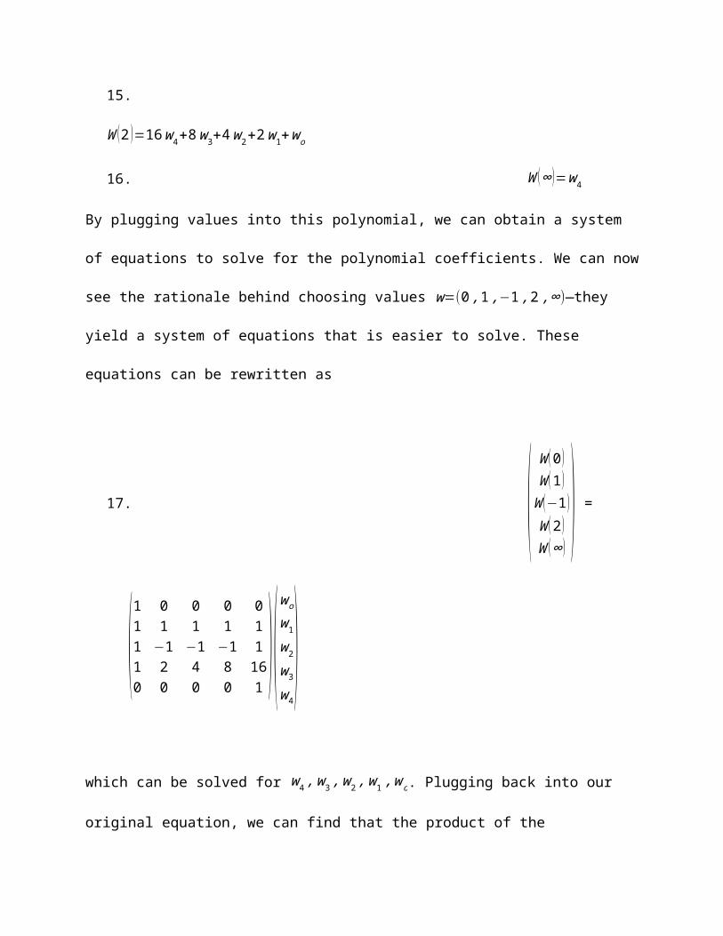
By plugging values into this polynomial, we can obtain a system of equations to solve for the

polynomial coefficients. We can now see the rationale behind choosing values

w=(0 ,1,−1 ,2 ,∞)—they yield a system of equations that is easier to solve. These equations can

be rewritten as

17. (W (0 )W (1 )W (−1 )W (2 )W (∞ )

) =(1 0 0 0 01 1 1 1 11 −1 −1 −1 11 2 4 8 160 0 0 0 1

)(wo

w1

w2

w3

w4

)

which can be solved for w4 ,w3 ,w2 ,w1 ,wo. Plugging back into our original equation, we can find

that the product of the multiplication is equal to 1012w4+109w3+106w2+103w 1+wo

CITATION Kro16¿1033(Kronenburg).

Toom-Cook Complexity

The Toom Cook 3-algorithm reduces a large multiplication to 5 multiplications of smaller

numbers. Thus, we can write:

18. M (n )=5M ( n3).

This implies that the Toom Cook 3-algorithm has a complexity of O (nlog3 5 )=O (n1.465 ).

In general, the Toom Cook k-algorithm has a complexity of O (nlogk2k−1 ). It is also interesting to

note that Karatsuba multiplication is actually a special case of the Toom Cook algorithm (Toom-

Cook 2-algorithm) and long multiplication is simply the Toom Cook 1-algorithm (Knuth).

Implementation:

Because the time-complexity of Karatsuba and Toom-Cook multiplication are both better

than that of long multiplication, they will become faster than long multiplication as input size

rises towards infinity. However, they are not necessarily more efficient than long multiplication

at all input sizes. There are several factors that contribute to this nuance. For instance, both

Karatsuba and Toom-Cook multiplication are slower than long multiplication at small inputs

because recursive overhead—the computing power required to recursively call a function several

times—will outweigh multiplicative efficiency when n is small. Therefore, implementations of

the Karatsuba and Toom-Cook algorithms often switch to long multiplication when the operands

in multiplication become small. In addition, for small inputs, the increase in number of additions

and subtractions outweighs the increased efficiency in multiplication, so long multiplication will

be more efficient. Lastly, solving the matrix equation in the Toom-Cook algorithm takes

computing power, and only becomes strategic for large inputs when the multiplicative efficiency

begins to outweigh the computing power required to solve the matrix equation. For even larger

numbers, algorithms such as the Schönhage–Strassen algorithm, which utilizes Fourier

Transformations, become more efficient (Knuth).

Division algorithm

Division can be understood as a multiplication between a dividend and the reciprocal of

the divisor. As a result, many division algorithms involve two steps: finding the reciprocal of the

dividend, and employing a multiplication algorithm to find the quotient.

To find the reciprocal of a number D, we can create an equation with root 1D and then

use Newton’s method to estimate the root. One equation that works is

19. f ( X )= 1X

−D.

Applying Newton’s method, we can iterate X i+1=X i−f (X i)f ' ( X i )

to find increasingly accurate

estimates of 1D. Each iteration of the algorithm can be given by the following:

20. X i+1=X i−

1X i

−D

−1X i

2

=X i(2−D X i).

Figure 2 gives a visual representation of Newton’s Method at work. Using the derivative of the

function, we find increasingly precise estimates of the root. We can quantity the accuracy of each

estimate using error analysis: if we define the error ϵ ito be X i−1D , the difference between the

actual value of 1D and our estimate, we find the error after each iteration of Newton’s Method.

However, using ϵ i=D X i−1, which is equivalent to the first expression multiplied by D, will

yield the same result with much cleaner math. We then calculate the error after an iteration of

Newton’s method.

ϵ i+1=D X i+1−1

¿2D X i−D2 X i2−1

¿−¿

¿−ϵ i2

This implies that each iteration of Newton’s method will result in roughly a doubling of the

number of correct digits in the result. After calculating the reciprocal of D to a sufficient degree

of accuracy, we can then use one of the aforementioned multiplication algorithms to find the

Figure 2: Newton’s Method

quotient. The use of Newton’s method to find the reciprocal of a dividend and then multiplying

the reciprocal by the divisor is known as the Newton-Raphson method. The time complexity of

finding the reciprocal is O (log (n ) F (n ) ) where F (n ) is the number of fundamental operations

needed to calculate the reciprocal to n-digit precision. Therefore, the overall time-complexity of

division will be the time complexity of the sum of operations needed to find the reciprocal and

multiply the reciprocal by the dividend: O (log (n ) F (n )+n1.465) = O (n1.465 ) since exponential

growth will eclipse the other term’s growth as input length approaches infinity. Therefore,

division will have the same asymptotic complexity as multiplication (Cook).

Like multiplication, the implementation of division algorithms will often be slower than

standard long division for small inputs due to recursive overhead. In addition, the computing

power used to calculate the reciprocal of an operand for small inputs would be more efficiently

utilized on simply carrying out the long division. Thus, like multiplication, the division algorithm

used by computers will depend on the input length. Typically, the Newton-Raphson algorithm is

only used for very large inputs (Papadimitriou).

Conclusion:

Currently, the fastest multiplication and division algorithm for two n digit integers

remains an open question in computer science. And yet, an increase in multiplication and

division efficiency could lead to significantly faster computing speeds and new capabilities to

process ever-increasing amounts of data.

Works Cited

Babai, Laszlo. "Divide and Conquer: The Karatsuba–Ofman algorithm." UChicago: Laszlo Babai. 3 Dec 2016 <http://people.cs.uchicago.edu/~laci/HANDOUTS/karatsuba.pdf>.

Bodrato, M. Zanoni. "Integer and Polynomial Multiplication: Towards Optimal Toom-Cook Matrices." Proceedings of the ISSAC 2007 Conference. New York: ACM press, 2007.

Cook, Stephen A. On the Minimum Computation Time of Functions. Cambridge, 1966.

Knuth, Donald. The Art of Computer Programming. Addison Wesley , 2005.

Kronenburg, M.J. Toom-Cook Multiplication: Some Theoretical and Practical Aspects. 16 Feb 2016.

Ofman, A. Karatsuba and Yu. "Multiplication of Many-Digital Numbers by Automatic Computers." Proceedings of the USSR Academy of Sciences. Physics-Doklady, 1963. 595–596.

Papadimitriou, Christos H. Computational complexity. Reading: Addison-Wesley, 1994.

Smith, Mark D. "Newton-Raphson Technique ." 1 Oct 1998. MIT 10.001. 6 Dec 2016 <http://web.mit.edu/10.001/Web/Course_Notes/NLAE/node6.html>.

Picture Bibliography

1. Graphed on https://www.desmos.com/

2. http://tutorial.math.lamar.edu/Classes/CalcI/NewtonsMethod_files/image001.gif