CloudVista: Visual Cluster Exploration for ExtremeScale Data in the Cloud

Keke Chen, Huiqi Xu, Fengguang Tian, Shumin Guo

Ohio Center of Excellence in Knowledge Enabled ComputingDepartment of Computer Science and EngineeringWright State University, Dayton, OH 45435, USA

{keke.chen, xu.39, tian.6, guo.18}@wright.edu

Abstract. The problem of efficient and high-quality clustering of extreme scaledatasets with complex clustering structures continues to be one of the most chal-lenging data analysis problems. An innovate use of data cloud would provideunique opportunity to address this challenge. In this paper, we propose the Cloud-Vista framework to address (1) the problems caused by using sampling intheexisting approaches and (2) the problems with the latency caused by cloud-sideprocessing on interactive cluster visualization. The CloudVista framework aimsto explore the entire large data stored in the cloud with the help of the data struc-turevisual frameand the previously developed VISTA visualization model. Thelatency of processing large data is addressed by theRandGenalgorithm that gen-erates a series of related visual frames in the cloud without user’s intervention,and a hierarchical exploration model supported by cloud-side subsetprocessing.Experimental study shows this framework is effective and efficient for visuallyexploring clustering structures for extreme scale datasets stored in the cloud.

1 Introduction

With continued advances in communication network technology and sensing technol-ogy, there is an astounding growth in the amount of data produced and made availablethroughout cyberspace. Cloud computing, the notion of outsourcing hardware and soft-ware to Internet service providers through large-scale storage and computing clusters,is emerging as a dominating technology and an economical wayto host and analyzemassive data sets. Data clouds, consisting of hundreds or thousands of cheap multi-corePCs and disks, are available for rent at low cost (e.g., Amazon EC2 and S3 services).Powered with distributed file systems, e.g., hadoop distributed file system [26], andMapReduce programming model [7], clouds can provide equivalent or better perfor-mance than traditional supercomputing environments for data intensive computing.

Meanwhile, with the growth of data volume, large datasets1 will often be gener-ated, stored, and processed in the cloud. For instance, Facebook stores and processesuser activity logs in hadoop clusters [24]; Yahoo! used hadoop clusters to process webdocuments and generate web graphs. To explore such large datasets, we have to de-velop novel techniques that utilize the cloud infrastructure and its parallel processing

1 The concept of “large data” keeps evolving. with existing scales of data,roughly, we consider< 10

3 records to be small,103 − 106 to be medium,106 − 10

9 to be large, and> 109 to be

extreme scale.

power. In this paper we investigate the problem of large-scale data clustering analysisand visualization through innovative use of the cloud.

1.1 Challenges with Clustering Extreme Scale Data

A clustering algorithm tries to partition the records into groups with certain similaritymeasure [15]. While a dataset can be large in terms of the number of dimensions (di-mensionality), the number of records, or both, a “large” web-scale data usually referto those having multi-millions, or even billions of records. For example, one-day websearch clickthrough log for a major commercial web search engine in US can have tensof millions of records. Due to the large volume of data, typical analysis methods arelimited to simple statistics based on linear scans. When high-level analysis methodssuch as clustering are applied, the traditional approacheshave to use data reductionmethods.

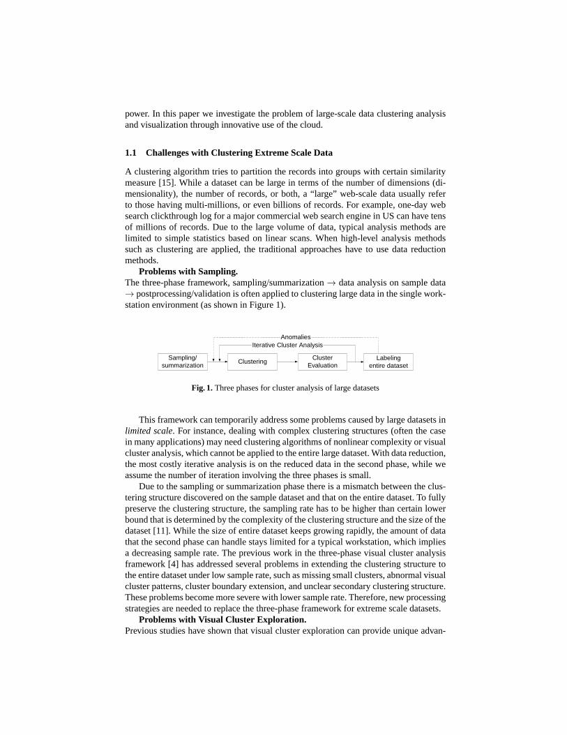
Problems with Sampling.The three-phase framework, sampling/summarization→ data analysis on sample data→ postprocessing/validation is often applied to clusteringlarge data in the single work-station environment (as shown in Figure 1).

Sampling/summarization

ClusteringCluster

Evaluation

Iterative Cluster Analysis

Labelingentire dataset

Anomalies

Fig. 1. Three phases for cluster analysis of large datasets

This framework can temporarily address some problems caused by large datasets inlimited scale. For instance, dealing with complex clustering structures(often the casein many applications) may need clustering algorithms of nonlinear complexity or visualcluster analysis, which cannot be applied to the entire large dataset. With data reduction,the most costly iterative analysis is on the reduced data in the second phase, while weassume the number of iteration involving the three phases issmall.

Due to the sampling or summarization phase there is a mismatch between the clus-tering structure discovered on the sample dataset and that on the entire dataset. To fullypreserve the clustering structure, the sampling rate has tobe higher than certain lowerbound that is determined by the complexity of the clusteringstructure and the size of thedataset [11]. While the size of entire dataset keeps growing rapidly, the amount of datathat the second phase can handle stays limited for a typical workstation, which impliesa decreasing sample rate. The previous work in the three-phase visual cluster analysisframework [4] has addressed several problems in extending the clustering structure tothe entire dataset under low sample rate, such as missing small clusters, abnormal visualcluster patterns, cluster boundary extension, and unclearsecondary clustering structure.These problems become more severe with lower sample rate. Therefore, new processingstrategies are needed to replace the three-phase frameworkfor extreme scale datasets.

Problems with Visual Cluster Exploration.Previous studies have shown that visual cluster exploration can provide unique advan-

tages over automated algorithms [3, 4]. It can help user decide the best number of clus-ters, identify some irregular clustering structures, incorporate domain knowledge intoclustering, and detect errors.

However, visual cluster exploration on the data in the cloudbrings extra difficulties.First, the visualization algorithm should be parallelizable. Classical visualization meth-ods such as Principal Component Analysis and projection pursuit [13] involve complexcomputation, not easy to scale to large data in the parallel processing environment.Second, cloud processing is not optimized for low-latency processing [7], such as in-teractive visualization. It would be inappropriate to respond to each user’s interactiveoperation with a cloud-based processing procedure, because the user cannot toleratelong waiting time after each mouse click. New visualizationand data exploration mod-els should be developed to fit the cloud-based data processing.

1.2 Scope and Contributions

We propose the cloud-based interactive cluster visualization framework,CloudVista,to address the aforementioned challenges for explorative cluster analysis in the cloud.The CloudVista framework aims to eliminate the limitation brought by the sampling-based approaches and reduce the impact of latency to the interactivity of visual clusterexploration.

Our approach explores the entire large data in the cloud to address the problemscaused by sampling. CloudVista promotes a collaborative framework between the datacloud and the visualization workstation. The large datasetis stored, processed in thecloud and reduced to a key structure “visual frame”, the sizeof which is only subjectto the resolution of visualization and much smaller than an extreme scale dataset. Vi-sual frames are generated in batch in the cloud, which are sent to the workstation. Theworkstation renders visual frames locally and supports interactive visual exploration.

The choice of the visualization model is the key to the success of the proposedframework. In the initial study, we choose our previously developed VISTA visualiza-tion model [3] for it has linear complexity and can be easily parallelized. The VISTAmodel has shown effectiveness in validating clustering structures, incorporating domainknowledge in previous studies [3] and handling moderately large scale data with thethree-phase framework [4].

We address the latency problem with an automatic batch framegeneration algo-rithm - the RandGen algorithm. The goal is to efficiently generate a series of mean-ingful visual frames without the user’s intervention. Withthe initial parameter settingdetermined by the user, the RandGen algorithm will automatically generate the param-eters for the subsequent visual frames, so that these framesare also continuously andsmoothly changed. We show that the statistical properties of this algorithm can helpidentify the clustering structure. In addition to this algorithm, we also support a hierar-chical exploration model to further reduce the cost and needof cloud-side processing.

We also implement a prototype system based on Hadoop/MapReduce [26] and theVISTA system [3]. Extensive experiments are conducted to study several aspects ofthe framework, including the advantages of visualizing entire large datasets, the per-formance of the cloud-side operations, the cost distribution between the cloud and theapplication server, and the impact of frame resolution to running time and visualiza-tion quality. The preliminary study on the prototype has shown that the CloudVista

framework works effectively in visualizing the clusteringstructures for extreme scaledatasets.

2 CloudVista: the Framework, Data Structure and Algorithms

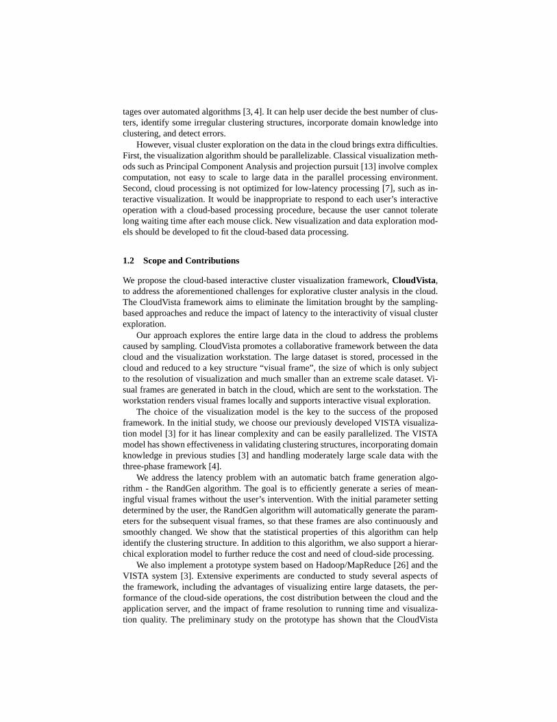
CloudVista works differently from existing workstation-based visualization. Workstation-based visualization directly processes each record and renders the visualization after thevisual parameters are set. In the CloudVista framework, we clearly divide the respon-sibilities between the cloud, the application server, and the client (Figure 2). The dataand compute intensive tasks on large datasets are now finished in the cloud, which willgenerate the intermediate visual representations - the visual frames (or user selectedsubsets). The application server manages the visual frame/subset information, issuescloud processing commands, gets the results from the cloud,compresses data for trans-mission, and delivers data to the client. The client will render the frames, take careof user interaction, and, if the selected subsets are small,work on these small subsetsdirectly with the local visualization system.

Hadoop Nodes AppServer������������ ����� � �� � ������ ������� � �� � ����� ��������� In the cloud

Client

Fig. 2. The CloudVista framework

We describe the framework in three components: the VISTA visualization model,the key data structure “visual frame”, and the major data processing and visualizationalgorithms. We will also include a cost analysis on cloud-side operations at the end ofthis section.

2.1 The VISTA Visualization Model

The CloudVista framework uses our previously developed VISTA visualization model[3] for it has linear complexity and can be easily parallelized. To make the paper self-contained, we describe the definition of this model and its properties for cluster visual-ization.

VISTA visualization model is used to map ak-dimensional point to a two di-mensional point on the display. Letsi ∈ R

2, i = 1, . . . , k be unit vectors arrangedin a “star shape” around the origin on the display.si can be represented assi =(cos(θi), sin(θi)), θi ∈ [0, 2π], i.e., uniquely defined byθi. Let ak-dimensional normal-ized data pointx = (x1, . . . xi, . . . , xk), xi ∈ [−1, 1] in the 2D space andu = (u1, u2)bex’s image on the two dimensional display based on the VISTA mapping function.

α = (α1, . . . , αk), αi ∈ [−1, 1] are dimensional weights andc ∈ R+ (i.e., positive

real) is a scaling factor. Formula 1 defines the VISTA model:

f(x, α, θ, c) = c

k∑

i=1

αixisi. (1)

αi, θi, andc provide the adjustable parameters for this mapping. For simplicity,we leaveθi to be fixed that equally partitions the circle, i.e.,θi = 2iπ/k. Experimentalresults showed that adjustingα in [−1, 1], combined with the scaling factorc is effectiveenough for finding satisfactory visualization [3, 4].

G(x) = Ax+b

Fig. 3. Use a Gaussian mixture to describe theclusters in the dataset.

This model is essentially a simple linear model with dimensional adjustable param-etersαi. The rationale behind the model is

Proposition 1 If Euclidean distance is used as the similarity measure, an affine map-ping does not break clusters but may cause cluster overlapping.

Proof. Let’s model arbitrary shaped clusters with a Gaussian mixture [8]. Letµ be thedensity center, andΣ be the covariance matrix of the Gaussian cluster. A clusterCi canbe represented with

Ni(µi, Σi) =1

(2π)k/2|Σi|1/2exp{−(x− µi)

′Σ−1(x− µi)/2}

Geometrically,µ describes the position of the cluster andΣ describes the spread of thedense area. After an affine transformation, sayG(x) = Ax+b, the center of the clusteris moved toAµi + b and the covariance matrix (corresponding to the shape of densearea) is changed toAΣiA

T . And the dense area is modeled withNi(Aµi+b, AΣiAT ).

Therefore, affine mapping does not break the dense area, i.e., the cluster. However, dueto the changed shapes of the clusters,AΣiA

T , some clusters may overlap each other.As the VISTA model is an affine model, this proposition also applies to the VISTAmodel.�

Since there is no “broken cluster” in the visualization, anyvisual gap between thepoint clouds reflects the real density gaps between the clusters in the original high-dimensional space. The only challenge is to distinguish thedistance distortion andcluster overlapping introduced by the mapping. Uniquely different from other mod-els, by tuningαi values, we can scrutinize the multidimensional dataset visually from

different perspectives, which gives dynamic visual clues for distinguishing the visualoverlapping2.

In addition, since this model is a record-based mapping function, it is naturallyparallel and can be implemented with the popular parallel processing models suchas MapReduce [7] for large scale cloud-based data processing. Therefore, we use theVISTA model in our framework. Note that our framework does not exclude using anyother visualization model if it can efficiently implement the functionalities.

2.2 The Visual Frame Structure

A key structure in CloudVista is thevisual framestructure. It encodes the visualizationand allows the visualization to be generated in parallel in the cloud side. It is also aspace-efficient data structure for passing the visualization from the cloud to the clientworkstation.

Since the visual representation is limited by display size,almost independent ofthe size of the original dataset, visualizing data is naturally a data reduction process.A rectangle display area for a normal PC display contains a fixed number of pixels,about one thousand by one thousand pixels3. Several megabytes will be sufficient torepresent the pixel matrix. In contrast, it is normal that a large scale dataset may easilyreach terabytes. When we transform the large dataset to a visual representation, a datareduction process happens, where the cloud computation model, e.g., MapReduce, cannicely fit in.

We design the visual representation based on the pixel matrix. The visual data reduc-tion process in our framework is implemented as an aggregation process. Concretely,we use a two dimensional histogram to represent the pixel matrix: each cell is an aggre-gation bucket representing the corresponding pixel or a number of neighboring pixels(which is defined by theResolution). All points are mapped to the cells and then ag-gregated. We name such a 2-D bucket structure as “visual frame”. A frame can bedescribed as a list of tuples〈u1, u2, d〉, where(u1, u2) is the coordinate of the cell andd > 0 records the number of points mapped to the cell. The buckets are often filledsparsely, which makes the actual size of a frame structure issmaller than megabytes.Low resolution frame uses one bucket representing a number of neighboring pixels,which also reduces the size of frame.

Such a visual frame structure is appropriate for density-based cluster visualization,e.g., those based on the VISTA model. The following MapReduce code snippet de-scribes the use of the visual frame based on the VISTA model.

The VISTA visualization model maps the dense areas in the original space to sep-arated or overlapped dense areas on the display. With small datasets, clusters are visu-alized as dense point clouds, where point-based visualization is sufficient for users todiscern clustering structures. With large datasets, all points are crowded together on thedisplay. As a result, point-based visualization does not work. We can use the widely

2 A well-known problem is that the VISTA model cannot visually separate some manifold struc-tures such nested spherical surfaces, which can be addressed by using spectral clustering [19]as the preprocessing step.

3 Note that special displays, such as NASA’s hyperwall-2, needs special hardware, which arenot available for common users, thus do not fit our research scope.

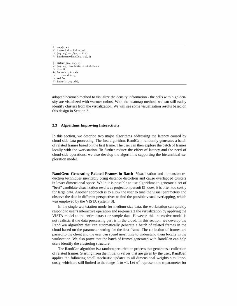
1: map(i,x)2: i: record id,x: k-d record.3: (u1, u2)← f(x, α, θ, c);4: EmitIntermediate((u1, u2), 1)

1: reduce((u1, u2), v)2: (u1, u2): coordinate,v: list of counts.3: d← 0;4: for eachvi in v do5: d← d + vi;6: end for7: Emit(〈u1, u2, d〉);

adopted heatmap method to visualize the density information - the cells with high den-sity are visualized with warmer colors. With the heatmap method, we can still easilyidentify clusters from the visualization. We will see some visualization results based onthis design in Section 3.

2.3 Algorithms Improving Interactivity

In this section, we describe two major algorithms addressing the latency caused bycloud-side data processing. The first algorithm, RandGen, randomly generates a batchof related frames based on the first frame. The user can then explore the batch of frameslocally with the workstation. To further reduce the effect of latency and the need ofcloud-side operations, we also develop the algorithms supporting the hierarchical ex-ploration model.

RandGen: Generating Related Frames in Batch Visualization and dimension re-duction techniques inevitably bring distance distortion and cause overlapped clustersin lower dimensional space. While it is possible to use algorithms to generate a set of“best” candidate visualization results as projection pursuit [5] does, it is often too costlyfor large data. Another approach is to allow the user to tune the visual parameters andobserve the data in different perspectives to find the possible visual overlapping, whichwas employed by the VISTA system [3].

In the single workstation mode for medium-size data, the workstation can quicklyrespond to user’s interactive operation and re-generate the visualization by applying theVISTA model to the entire dataset or sample data. However, this interactive model isnot realistic if the data processing part is in the cloud. In this section, we develop theRandGen algorithm that can automatically generate a batch of related frames in thecloud based on the parameter setting for the first frame. The collection of frames arepassed to the client and the user can spend most time to understand them locally in theworkstation. We also prove that the batch of frames generated with RandGen can helpusers identify the clustering structure.

The RandGen algorithm is a random perturbation process thatgenerates a collectionof related frames. Starting from the initialα values that are given by the user, RandGenapplies the following small stochastic updates to all dimensional weights simultane-ously, which are still limited to the range -1 to +1. Letαφ

i represent theα parameter for

dimensioni in frameφ, the new parameterαφ+1i is defined randomly as follows.

δi = t×B,

αφ+1i =

1 if αφi + δi > 1

αφi + δ if αφ

i + δi ∈ [−1, 1]

−1 if αφi + δi < −1,

(2)

wheret is a predefined step length, often set to small, e.g.,0.01 ∼ 0.05, andB is acoin-tossing random variable - with probability 0.5 it returns 1 or -1.δi is generatedindependently at random for each dimension.αφ+1

i is also bounded by the range [-1,1]to minimize the out-of-bound points (those mapped out of thedisplay). This processrepeats until theα parameters for a desired number of frames are generated. Since theadjustment at each step is small, the change between the neighboring frames is smalland smooth. As a result, sequentially visualized these frames will create continuouslychanging visualization. The following analysis shows why the RandGen algorithm canhelp identify visual cluster overlapping.

Identifying Clustering Patterns with RandGen.We formally analyze why this ran-dom perturbation process can help us identify the clustering structure. The change ofvisualization by adjustingα values can be described by the random movement of eachvisualized point. Letv1 andv2 be the images of the original data recordx for the twoneighboring frames, respectively. Then, the point movement is represented as

∆u = c

k∑

i=1

δixisi.

By definition ofB, we haveE[δi] = 0. Sinceδi are independent of each other, wederive the expectation ofδiδj

E[δiδj ] = E[δi]E[δj ] = 0, for i 6= j.

Thus, it follows the expectation of point movement is zero:E[∆u] = 0. That means thepoint will randomly move around the initial position. Let the coordinatesi be(si1, si2).We can derive the variance of the movement var(∆u) =

c2t2var(B)

(

∑ki=1 x

2i s

2i1

∑ki=1 x

2i si1si2

∑ki=1 x

2i si1si2

∑ki=1 x

2i s

2i2

)

(3)

There are a number of observations based on the variance. (1)The larger the step lengtht, the more actively the point moves; (2) As the valuessix andsiy are shared by allpoints, the points with larger vector length

∑ki=1 x

2i tends to move more actively.

Since we want to identify cluster overlapping by observing point movements, it ismore interesting to see how the relative positions change for different points. Letw1

andw2 be the images of another original data recordy for the neighboring frames,respectively. With the previous definition ofx, the visual squared distance between thepair of points in the initial frame would be

∆(1)w,v = ||w1 − v1||

2 = ||ck∑

i=1

αi(xi − yi)si||2. (4)

Then, the change of the squared distance between the two points is

∆w,v = 1/c2(∆(2)w,v −∆(1)

w,v)

= (∑

i=1

δi(xi − yi)si1)2 + (

∑

i=1

δi(xi − yi)si2)2

+ 2(∑

i=1

δi(xi − yi)si1)(∑

i=1

αi(xi − yi)si1)

+ 2(∑

i=1

δi(xi − yi)si2)(∑

i=1

αi(xi − yi)si2).

With the independence betweenδi andδj for i 6= j, E(δi) = 0, s2i1 + s2i2 = 1, andE2[δi] = t2var(B) = 0.25t2, it follows the expectation of the distance change is

E[∆w,v] =

k∑

i=1

E2[δi](xi − yi)2 = 0.25t2

k∑

i=1

(xi − yi)2

where , i.e., the average change of distance is proportion tothe original distance be-tween the two points. That means, if points are distant in theoriginal space, we willhave higher probability to see them distant in the visual frames; if the points are close inthe original space, we will more likely observe them move together in the visual frames.This dynamics of random point movement helps us identify possible cluster overlappingin a series of continuously changing visual frames generated with the RandGen method.

Bootstrapping RandGen and Setting the Number of Frames.One may ask howto determine the initial set ofα parameters for RandGen. We propose a bootstrappingmethod based on sampling. In the bootstrapping stage, the cloud is asked to draw anumber of samples uniformly at random (µ records, defined by the the user accordingto the client side’s visual computing capacity). The user then locally explores the smallsubset to determine an interesting visualization, theα parameters of which are sent backfor RandGen. Note that this step is used to explore the sketchof the clustering structure.Therefore, the problems with sampling we mentioned in Introduction are not important.

Another question is how many frames are appropriate in a batch for the RandGenalgorithm. The goal is to have sufficient number of frames so that one batch is sufficientfor finding the important cluster visualization for a selected subset (see the next sec-tion for the extended exploration model), but we also do not want to waste computingresources to compute excessive frames. In the initial study, we found this problem is so-phisticated because it may involve the proper setting of thestep lengtht, the complexityof the clustering structure, and the selection of the initial frame. In experiments, we willsimply use 100 frames per batch. Thorough understanding of this problem would be animportant task for our future work.

Supporting Hierarchical Exploration A hierarchical exploration model allows theuser to interactively explore the detail of any part of the dataset based on the currentvisual frame. Such an exploration model can also exponentially reduce the data to beprocessed and the number of operations to be performed in thecloud side.

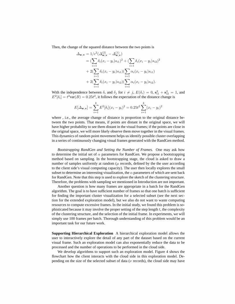
We develop algorithms to support such an exploration model.Figure 4 shows theflowchart how the client interacts with the cloud side in thisexploration model. De-pending on the size of the selected subset of data (ν records), the cloud side may have

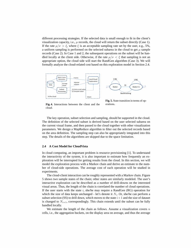
different processing strategies. If the selected data is small enough to fit in the client’svisualization capacity, i.e.,µ records, the cloud will return the subset directly (Case 1).If the rateµ/ν > ξ, whereξ is an acceptable sampling rate set by the user, e.g., 5%,a uniform sampling is performed on the selected subarea in the cloud to getµ samplerecords (Case 2). In Case 1 and 2, the subsequent operations on the subset will be han-dled locally at the client side. Otherwise, if the rateµ/ν < ξ that sampling is not anappropriate option, the cloud side will start the RandGen algorithm (Case 3). We willformally analyze the cloud-related cost based on this exploration model in Section 2.4.

Batch Frame

Generation

Subset

Processing

Data(3) large

subset

Local Visual

Exploration

Frames

Selected

subarea

(1) Entire small subset

(2) Sampled subset

In the cloud Client

Fig. 4. Interactions between the client and thecloud.

State i State i+1

1 RG

SS

Backtracking

1 RG

Fig. 5. State transition in terms of op-erations.

The key operation, subset selection and sampling, should besupported in the cloud.The definition of the selected subset is derived based on the user selected subarea onthe current visual frame, and then passed to the cloud together with other visualizationparameters. We design a MapReduce algorithm to filter out theselected records basedon the area definition. The sampling step can also be appropriately integrated into thisstep. The details of the algorithms are skipped due to the space limitation.

2.4 A Cost Model for CloudVista

In cloud computing, an important problem is resource provisioning [1]. To understandthe interactivity of the system, it is also important to estimate how frequently an ex-ploration will be interrupted for getting results from the cloud. In this section, we willmodel the exploration process with a Markov chain and derivean estimate to the num-ber of cloud-side operations. The average cost of each operation will be studied inexperiments.

The cloud-client interaction can be roughly represented with a Markov chain. Figure5 shows two sample states of the chain; other states are similarly modeled. The user’sinteractive exploration can be described as a number of drill-downs on the interestedvisual areas. Thus, the length of the chain is correlated thenumber of cloud operations.If the user starts with the statei, she/he may require a RandGen (RG) operation forwhich the size of data keeps unchanged - let’s denote itNi. Or, she/he can perform asubset selection (SS) to drill down, which moves to the statei+1 and the size of datasetis changed toNi+1, correspondingly. This chain extends until the subset can be fullyhandled locally.

We estimate the length of the chain as follows. Assume a visualization coversncells, i.e., the aggregation buckets, on the display area onaverage, and thus the average

density of the cells isNi/n for statei. We also assume the area the user may select forsubsect exploration is aboutλ percentage of then cells. So the size of data at statei+1is Ni+1 ≈ λNi. It follows Ni+1 = λi+1N0. We have defined the client’s visualizationcapacityµ and the acceptable sampling rateξ. For Ni+1 records to be handled fullylocally by the client, the boundary condition will beNi > µ/ξ andNi+1 ≤ µ/ξ.PluggingNi+1 = λi+1N0 into the inequalities, we get

logλµ

ξN0− 1 ≤ i < logλ

µ

ξN0,

i.e., i = ⌊logλµ

ξN0

⌋. Let the critical value beρ = i + 1. Assume only one RandGenwith sufficient number of frames is needed for each state. Since the number of interest-ing subareas for each level are quite limited, denoted byκ, the total number of cloudoperations isO(κρ).A concrete example may help us better understand the numberρ. Assume the client’s visualization capacity is 50,000 records, there are 500 millionrecords in the entire dataset, the acceptable sampling rateis 5%, and each time we se-lect about20% visual area, i.e.,λ = 0.2, to drill down. We getρ = 4. Therefore, thenumber of interrupts caused by cloud operations can be quiteacceptable for an extremescale dataset.

3 Experiments

The CloudVista framework addresses the sampling problem with the method of explor-ing whole dataset, and the latency problem caused by cloud data processing with theRandGen algorithm and the hierarchical exploration model.We conduct a number ofexperiments to study the unique features of the framework. First, we show the advan-tages of visualizing the entire large data, compared to the visualization of sample data.Second, we investigate how the resolution of the visual frame may affect the quality ofvisualization, and whether the RandGen can generate usefulframes. Third, we presentthe performance study on the cloud operations. The client-side visual exploration sys-tem (the VISTA system) has been extensively studied in our previous work [3, 4]. Thus,we skip the discussion on the effectiveness of VISTA clusterexploration, although theframe-based exploration will be slightly different.

3.1 Setup

The prototype system is setup in the in-house hadoop cluster. This hadoop cluster has 16nodes: 15 worker nodes and 1 master node. The master node alsoserves as the applica-tion server. Each node has two quad-core AMD CPUs, 16 GB memory, and two 500GBhard drives. These nodes are connected with a gigabit ethernet switch. Each workernode is configured with eight map slots and six reduce slots, approximately one mapslot and one reduce slot per core as recommended in the literature. The client desktopcomputer can comfortably handle about 50 thousands recordswithin 100 dimensionsas we have shown [4].

To evaluate the ability of processing large datasets, we extend two existing largescale datasets to larger scale for experiments. The following data extension method isused to preserve the clustering structure for any extensionsize. First, we replace the

categorical attributes (for KDD Cup data) with a sequence ofintegers (starting from0), and then normalize each dimension4. For a randomly selected record from the nor-malized dataset, we add a random noise (e.g., with normal distributionN(0, 0.01)) toeach dimensional value to generate a new record and this process repeats for sufficienttimes to get the desired number of records. In this way the basic clustering structure ispreserved in the extended datasets. The two original datasets are (1)Census 1990 datawith 68 attributes and (2)KDD Cup 1999 data with 41 attributes. The KDD Cup dataalso includes an additional label attribute indicating theclass of each record. We denotethe extended datasets with Censusext and KDDext respectively.

3.2 Visualizing the Whole Data

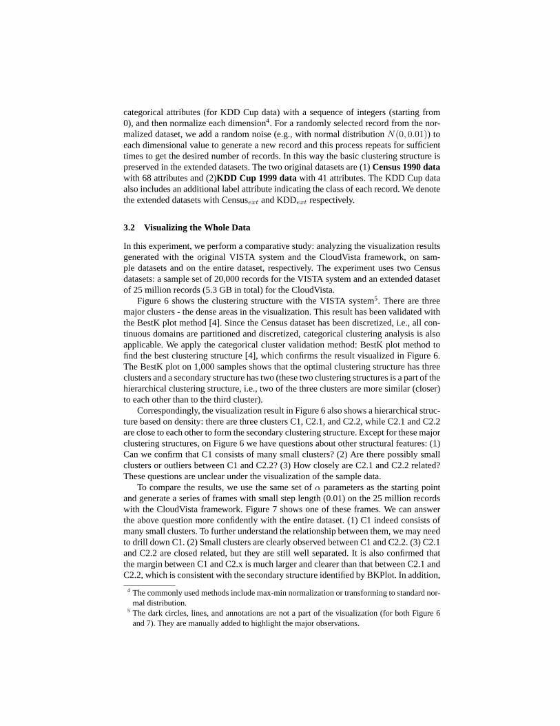
In this experiment, we perform a comparative study: analyzing the visualization resultsgenerated with the original VISTA system and the CloudVistaframework, on sam-ple datasets and on the entire dataset, respectively. The experiment uses two Censusdatasets: a sample set of 20,000 records for the VISTA systemand an extended datasetof 25 million records (5.3 GB in total) for the CloudVista.

Figure 6 shows the clustering structure with the VISTA system5. There are threemajor clusters - the dense areas in the visualization. This result has been validated withthe BestK plot method [4]. Since the Census dataset has been discretized, i.e., all con-tinuous domains are partitioned and discretized, categorical clustering analysis is alsoapplicable. We apply the categorical cluster validation method: BestK plot method tofind the best clustering structure [4], which confirms the result visualized in Figure 6.The BestK plot on 1,000 samples shows that the optimal clustering structure has threeclusters and a secondary structure has two (these two clustering structures is a part of thehierarchical clustering structure, i.e., two of the three clusters are more similar (closer)to each other than to the third cluster).

Correspondingly, the visualization result in Figure 6 alsoshows a hierarchical struc-ture based on density: there are three clusters C1, C2.1, andC2.2, while C2.1 and C2.2are close to each other to form the secondary clustering structure. Except for these majorclustering structures, on Figure 6 we have questions about other structural features: (1)Can we confirm that C1 consists of many small clusters? (2) Arethere possibly smallclusters or outliers between C1 and C2.2? (3) How closely areC2.1 and C2.2 related?These questions are unclear under the visualization of the sample data.

To compare the results, we use the same set ofα parameters as the starting pointand generate a series of frames with small step length (0.01)on the 25 million recordswith the CloudVista framework. Figure 7 shows one of these frames. We can answerthe above question more confidently with the entire dataset.(1) C1 indeed consists ofmany small clusters. To further understand the relationship between them, we may needto drill down C1. (2) Small clusters are clearly observed between C1 and C2.2. (3) C2.1and C2.2 are closed related, but they are still well separated. It is also confirmed thatthe margin between C1 and C2.x is much larger and clearer thanthat between C2.1 andC2.2, which is consistent with the secondary structure identified by BKPlot. In addition,

4 The commonly used methods include max-min normalization or transforming to standard nor-mal distribution.

5 The dark circles, lines, and annotations are not a part of the visualization(for both Figure 6and 7). They are manually added to highlight the major observations.

C1: may have substructures

Some high density cells: outliers, or the connection between C1 and C2?

C2.1 C2.2

Possible overlapping between C2 and C3

Secondary clustering structure identified by BKPlot

alpha axis

alpha widgit

Fig. 6. Visualization and Analysis of Censusdata with the VISTA system.

C1

Some high density small clusters/outliers

C2.1C2.2

C2 and C3 are close but well separated

Secondary clustering structure identified by BKPlot is confirmed:Close C2 and C3 could form a larger cluster

Confirmed Subclusters in C1

New discovery!Subclusters inC2.2

Fig. 7. Visualization and Analysis of 25 Mil-lion Census records (in 1000x1000 resolu-tion).

we also find some small sub-clusters inside C2.2, which cannot be observed in Figure6.

We summarize some of the advantages of visualizing entire large data. First, it canbe used to identify the small clusters that are often undetectable with sample dataset;Second, it helps identifying delicate secondary structures that are unclear in sampledata. Sample data has its use in determining the major clustering structure.

3.3 Usefulness of Frames Generated by RandGen

We have shown the statistical properties of the RandGen algorithm. In a sufficient num-ber of randomly generated frames by RandGen, the user will find the clustering patternin the animation created by playing the frames and distinguish potential visual clusteroverlaps. We conduct experiments on both the Censusext and KDDext datasets with thebatch size set to 100 frames. Both the random initial frame and the bootstrapping ini-tial frame are used in the experiments. We found in five runs ofexperiments, with thisnumber of frames, we could always find satisfactory visualization showing the mostdetailed clustering structure. The video at http://tiny.cc/f6d4g shows how the visual-ization of Censusext (with 25 millions of records) changes by playing the 100 framescontinuously.

3.4 Cost Evaluation on Cloud-Side Data Processing

In this set of experiments, we study the cost of the two major cloud operations: theRandGen algorithm and subset processing. We also analyze the cost distribution be-tween the cloud and the app server.

Lower resolution can significantly reduce the size of the frame data, but it may misssome details. Thus, it represents a potential tradeoff between system performance and

������������ �� �� �� ����� !"#$�%&�' ()*+,-./ -,0.-12 3*4554.627

�� 89:;<=>?�� 89:;<=>?��� 89:;<=>?Fig. 8. Running time vs data sizefor Censusext data (RandGen for 100frames).

@A@@B@@C@@D@@B@ D@ E@ F@ A@@GHIJKLMNHOPIQ RSTUVWXY Z[\S]^ YW]TV\

AB_`aa`bc defbdghBD _`aa`bc defbdghCE _`aa`bc defbdghFig. 9. Running time vs the number offrames for Censusext data.

ijikiikjiliiljimiinopqrqsotu vwwnrxsotuyz{|}~��z��{� ���� ������������� ����������

Fig. 10. Cloud processing time vs res-olutions for RandGen (100 frames,Censusext: 25 Million records, KDD-Cup ext: 40 Million records).

����������������������������� ¡�¢ £¤¥¦§¨©©ª¤«¬§­«©®¨§Fig. 11. Cost breakdown (data transfer+ compression) in app server process-ing (100 frames, Census-*: 25 Mil-lion records, KDDCup-*: 40 Millionrecords, *-high: 1000x1000 resolution,*-low: 250x250 resolution).

visual quality. Figure 7 in previous discussion is generated with 1000x1000 resolution,i.e., 1 aggregation cell for 1 pixel. Comparing with the result of 250x250 resolution,we find the visual quality is slightly reduced, but the major clustering features are wellpreserved for the Censusext data. Reducing resolution could be an acceptable methodto achieve better system performance. We will also study theimpact of resolution to theperformance.

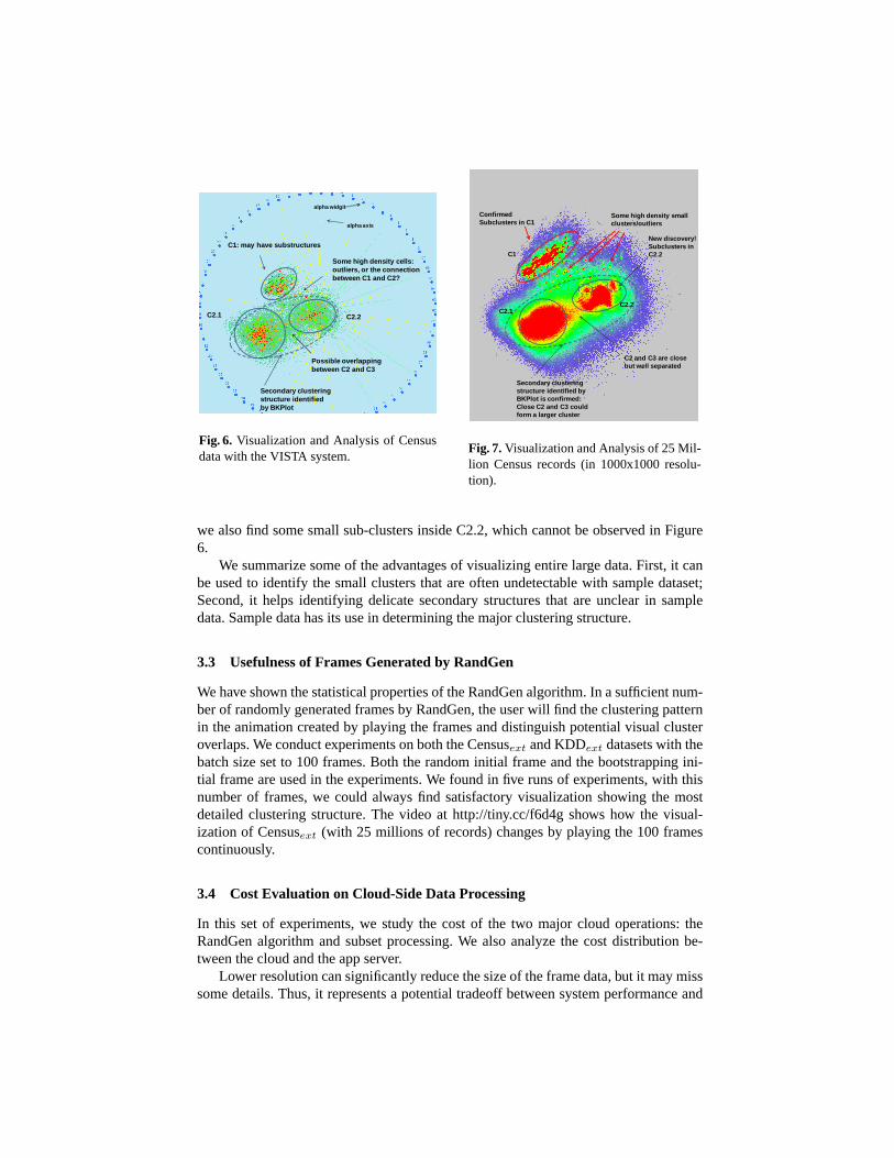
RandGen: Figure 8 demonstrates the running time of MapReduce RandGenalgo-rithm with different settings of map slots for the extended census data. We control thenumber of map slots with Hadoop’s fair scheduler. We set 100 reduces corresponding to100 frames in a batch for all the testing cases6. Note that each number in the figures isthe average of 5 test runs. The variance is small compared to the average cost and thusignored in the figures. The running time shows that the MapReduce RandGen algorithmis about linearly scalable in term of data size. With increasing number of map slots, the

6 We realized this is not an optimal setting, as only 90 reduce slots available in thesystem, whichmeans 100 reduce processes need to be scheduled in two rounds in the reduce phase.

cost also decreases proportionally. Figure 9 shows the costalso increases about linearlywithin the range of 100 frames.

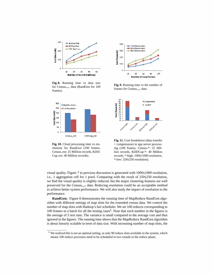
We then study the cost distribution at the server side (cloud+ application server).The total cost is split into three parts: cloud processing, transferring data to app serverfrom the cloud, and compressing. The following settings areused in this experiment.For RandGen of 100 frames, we compare two extended datasets:25 million recordsof Census (Censusext) data and 40 million records of KDD Cup (KDDext) data on 15worker nodes. The results are generated in two resolutions:1000x1000 (aggregationbucket is 1x1 pixel) and 250x250 (aggregation bucket is 4x4 pixels), respectively. Sincethe cloud processing cost dominates the total cost, we present the costs in two figures.Figure 10 shows the cost of cloud processing. KDDext takes more time since its datasize is much larger. Also, lower resolution saves a significant amount of time. Figure 11shows the cost breakdown at the app server, where the suffixesof the x-axis names: “-L”and “-H” mean low and high resolutions, respectively. Interestingly, although KDDextdata takes more time in cloud processing, it actually returns less data in frames, whichimplies a smaller number of cells are covered by the mapped points. By checking thehigh-resolution frames, we found there are about 320 thousands of covered cells perframe for census data, while only 143 thousands for KDD cup data, which results in thecost difference in app server processing.

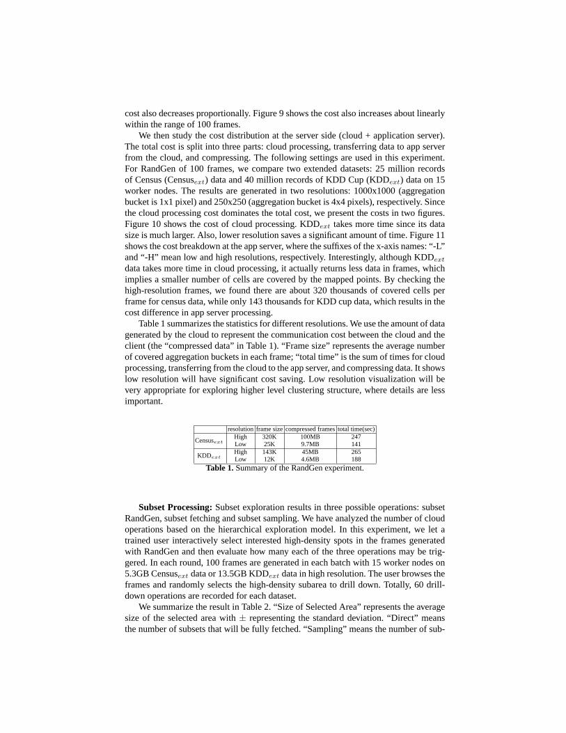
Table 1 summarizes the statistics for different resolutions. We use the amount of datagenerated by the cloud to represent the communication cost between the cloud and theclient (the “compressed data” in Table 1). “Frame size” represents the average numberof covered aggregation buckets in each frame; “total time” is the sum of times for cloudprocessing, transferring from the cloud to the app server, and compressing data. It showslow resolution will have significant cost saving. Low resolution visualization will bevery appropriate for exploring higher level clustering structure, where details are lessimportant.

resolutionframe sizecompressed framestotal time(sec)

Censusext

High 320K 100MB 247Low 25K 9.7MB 141

KDDext

High 143K 45MB 265Low 12K 4.6MB 188

Table 1. Summary of the RandGen experiment.

Subset Processing: Subset exploration results in three possible operations: subsetRandGen, subset fetching and subset sampling. We have analyzed the number of cloudoperations based on the hierarchical exploration model. Inthis experiment, we let atrained user interactively select interested high-density spots in the frames generatedwith RandGen and then evaluate how many each of the three operations may be trig-gered. In each round, 100 frames are generated in each batch with 15 worker nodes on5.3GB Censusext data or 13.5GB KDDext data in high resolution. The user browses theframes and randomly selects the high-density subarea to drill down. Totally, 60 drill-down operations are recorded for each dataset.

We summarize the result in Table 2. “Size of Selected Area” represents the averagesize of the selected area with± representing the standard deviation. “Direct” meansthe number of subsets that will be fully fetched. “Sampling”means the number of sub-

sets that can be sampled. “SS-RG” means the number of subsets, the sizes of whichare too large to be sampled - the system will perform a subset RandGen to preservethe structure. “D&S Time” is the average running time (seconds) for each “Direct” or“Sampling” operation in the cloud side processing, excluding the cost of SS-RG, sincewe have evaluated the cost of RandGen in Table 1.

Size of Selected Area# of Cloud Operations

D&S Time(sec)Direct SamplingSS-RG

Censusext 13896± 17282 4 34 22 36KDDext 6375±9646 9 33 18 43

Table 2. Summary of the subsect selection experiment.

Interestingly, the selected areas are normally small: on average about 4% of theentire covered area for both datasets. Most selections, specifically, 63% for Censusextand 70% for KDDext data, can be handled by “Direct” and “Sampling” and their costsare much less than RandGen.

4 Related Work

Most existing cluster visualization methods cannot scale up to large datasets due to theirvisual design. Parallel Coordinates [14] uses lines to represent multidimensional points.With large data, the lines are stacked together, clutteringthe visual space. Its visualdesign also does not allow a large number of dimensions to be visualized. Scatter plotmatrix and HD-Eye [12] are based on density-plots of pairwise dimensions, which arenot convenient for finding the global clustering structure and are not scale to the numberof dimensions. Star Coordinates [16] and VISTA [3] models are point-based modelsand have potential to be extended to handle really large datasets - the work describedin the paper is based on the VISTA visualization model. IHD [27] and HierarchicalClustering Explorer [23] are used to visualize the clustering structures discovered byclustering algorithms, which are different from our purpose of using the visualizationsystem to discover clusters.

Cluster visualization is also a dimensionality reduction problem in the sense that itmaps the original data space to the two dimensional visual space. The popularly useddimensionality reduction algorithms such as Principal Component Analysis and Mul-tidimensional Scaling [6] have been applied in visualization. These methods, togetherwith many dimensionality reduction algorithms [21, 22], are often costly - nonlinearto the number of records and thus they are not appropriate forlarge datasets. FastMap[9] addresses the cost problem for large datasets, but the choice of pivot points in themapping may affect the quality of the result. Random projection [25] only preservespairwise distances approximately on average and the precision is subject to the numberof projected dimensions - the lower projected dimensions the worse precision. Mostimportantly, all of these dimensionality reduction methods do not address the commonproblems - how to detect and understand distance distortionand cluster overlapping.The projection-based methods such as Grand Tour and Projection Pursuit [5] allow theuser to interactively explore multiple visualizations to discover possible distance distor-tion and cluster overlapping, but they are too costly to be used for large datasets. The

family of star coordinates systems [16, 3] address the visual distortion problem with amore efficient way, which is also the basis of our approach. The advantage of stochas-tic animation in finding patterns, as we do with RandGen, is also explored in graphvisualization [2]

The three-phase framework “sampling or summarization – clustering/cluster analy-sis – disk labeling” is often used to incorporate the algorithms of high time complexityin exploring large datasets. As the size of data grows to verylarge, the rate between thesize of the sampled or summarized dataset to the original size becomes very small, af-fecting the fidelity of the preserved clustering structure.Some clustering features suchas small clusters and the connection between closely related clusters are not easy to bediscovered with the sample set [4]. Therefore, there is a need to explore the entire largedataset.

Recently, several data mining algorithms have been developed in the cloud, show-ing that the hadoop/MapReduce [7] infrastructure is capable to reliably and efficientlyhandle large-scale data intensive problems. These instances include PLANET [20] fortree ensemble learning, PEGASUS [17] for mining peta-scalegraphs, and text miningwith MapReduce [18]. There is also an effort on visualizing scientific data (typically,low dimensional) with the support of the cloud [10]. However, none has been reportedon visualizing multidimensional extreme scale datasets inthe cloud.

5 Conclusion

The existing three-phase framework for cluster analysis onlarge scale data has reachedits limits for extreme scale datasets. The cloud infrastructure provides a unique oppor-tunity to address the problem of scalable data analysis - terabytes or even petabytes ofdata can be comfortably processed in the cloud. In this paper, we propose the Cloud-Vista framework to utilize the ability of scalable parallelprocessing power of the cloud,and address the special requirement of low-latency for user-centered visual analysis.We have implemented the prototype system based on the VISTA visualization modeland Hadoop/MapReduce. In experiments, we carefully evaluate the unique advantagesof the framework for analyzing the entire large dataset and the performance of cloud-side algorithms. The initial results and the prototype system have shown this frameworkworks effectively for exploring large datasets in the cloud. As a part of the future work,we will continue to study the setting of the batch size for RandGen and experiment withlarger hadoop cluster.

References

1. M. Armbrust, A. Fox, R. Griffith, A. D. Joseph, R. Katz, A. Konwinski, G. Lee, D. Patterson,A. Rabkin, I. Stoica, and M. Zaharia. Above the clouds: A berkeley viewof cloud computing.Technical Report, University of Berkerley, 2009.

2. J. Bovey, P. Rodgers, and F. Benoy. Movement as an aid to understanding graphs. InIEEEConference on Information Visualization, pages 472–478. IEEE, 2003.

3. K. Chen and L. Liu. VISTA: Validating and refining clusters via visualization. InformationVisualization, 3(4):257–270, 2004.

4. K. Chen and L. Liu. iVIBRATE: Interactive visualization based framework for clusteringlarge datasets.ACM Transactions on Information Systems, 24(2):245–292, 2006.

5. D. Cook, A. Buja, J. Cabrera, and C. Hurley. Grand tour and projection pursuit.Journal ofComputational and Graphical Statistics, 23:155–172, 1995.

6. T. F. Cox and M. A. A. Cox.Multidimensional Scaling. Chapman&Hall/CRC, Boca Raton,FL, US, 2001.

7. J. Dean and S. Ghemawat. MapReduce: Simplified data processing onlarge clusters. InUSENIX Symposium on Operating Systems Design and Implementation, 2004.

8. M. J. (editor). 1998.9. C. Faloutsos and K.-I. D. Lin. FastMap: A fast algorithm for indexing, data-mining and

visualization of traditional and multimedia datasets. InProceedings of ACM SIGMOD Con-ference, pages 163–174, 1995.

10. K. Grochow, B. Howe, R. Barga, and E. Lazowska. Client + cloud: Seamless architecturesfor visual data analytics in the ocean sciences. InProceedings of International Conferenceon Scientific and Statistical Database Management (SSDBM), 2010.

11. S. Guha, R. Rastogi, and K. Shim. CURE: An efficient clustering algorithm for largedatabases. InProceedings of ACM SIGMOD Conference, pages 73–84, 1998.

12. A. Hinneburg, D. A. Keim, and M. Wawryniuk. Visual mining of high-dimensional data. InIEEE Computer Graphics and Applications, pages 1–8, 1999.

13. P. J. Huber. Projection pursuit.Annals of Statistics, 13(2):435–475, 1985.14. A. Inselberg. Multidimensional detective. InIEEE Symposium on Information Visualization,

pages 100–107, 1997.15. A. Jain, M. Murty, and P. Flynn. Data clustering: A review.ACM Computing Surveys,

31:264–323, 1999.16. E. Kandogan. Visualizing multi-dimensional clusters, trends, and outliers using star coordi-

nates. InProceedings of ACM SIGKDD Conference, pages 107–116, 2001.17. U. Kang, C. E. Tsourakakis, and C. Faloutsos. Pegasus: Mining peta-scale graphs.Knowl-

edge and Information Systems (KAIS), 2010.18. J. Lin and C. Dyer.Data-intensive text processing with MapReduce. Morgan & Claypool

Publishers, 2010.19. A. Y. Ng, M. I. Jordan, and Y. Weiss. On spectral clustering: Analysis and algorithm. In

Proceedings Of Neural Information Processing Systems (NIPS), 2001.20. B. Panda, J. S. Herbach, S. Basu, and R. J. Bayardo. Planet: Massively parall learning of tree

ensembles with mapreduce. InProceedings of Very Large Databases Conference (VLDB),2009.

21. S. T. Roweis and L. K. Saul. Nonlinear dimensionality reduction by locally linear embed-ding. Science, 290(5500):2323–2326, 2000.

22. L. K. Saul, K. Q. Weinberger, F. Sha, J. Ham, and D. D. Lee. Spectral methods for dimen-sionality reduction. InSemi-supervised Learning. MIT Press, 2006.

23. J. Seo and B. Shneiderman. Interactively exploring hierarchicalclustering results.IEEEComputer, 35(7):80–86, 2002.

24. A. Thusoo, Z. Shao, S. Anthony, D. Borthakur, N. Jain, J. Sen Sarma, R. Murthy, and H. Liu.Data warehousing and analytics infrastructure at facebook. InProceedings of ACM SIGMODConference, pages 1013–1020. ACM, 2010.

25. S. S. Vempala.The Random Projection Method. American Mathematical Society, 2005.26. T. White.Hadoop: The Definitive Guide. O’Reilly Media, 2009.27. J. Yang, M. O. Ward, and E. A. Rundensteiner. Interactive hierarchical displays: a general

framework for visualization and exploration of large multivariate datasets. Computers andGraphics Journal, 27:265–283, 2002.