Clouds and the Earth's Radiant Energy System€¦ · Web view · 2011-09-08The Clouds and the...

Clouds and the Earth's Radiant Energy System (CERES)

Data Management System

Product Name (Acyonym) Collection Document

Release 1Version 1

Primary Authors

SSAI people

Science Systems and Applications, Inc. (SSAI)One Enterprise Parkway, Suite 200

Hampton, VA 23666

DMO people

NASA Langley Research CenterClimate Science Branch

Science DirectorateBuilding 1250

21 Langley BoulevardHampton, VA 23681-2199

September 2011

XYZ Collection Guide 9/8/2011

Document Revision Record

The Document Revision Record contains information pertaining to approved document changes. The table lists the date the Software Configuration Change Request (SCCR) was approved, the Release and Version Number, the SCCR number, a short description of the revision, and the revised sections. The document authors are listed on the cover. The Head of the CERES Data Management Team approves or disapproves the requested changes based on recommendations of the Configuration Control Board.

Document Revision Record

SCCRApproval

Date

Release/VersionNumber

SCCRNumber Description of Revision Section(s)

Affected

xx/xx/11 R1V1 xxx Initial draft document. All

ii


PrefaceThe Clouds and the Earth’s Radiant Energy System (CERES) Data Management System supports the data processing needs of the CERES Science Team research to increase understanding of the Earth’s climate and radiant environment. The CERES Data Management Team works with the CERES Science Team to develop the software necessary to implement the science algorithms. This software, being developed to operate at the Langley Atmospheric Sciences Data Center (ASDC), produces an extensive set of science data products.

The Data Management System consists of 12 subsystems; each subsystem represents one or more stand-alone executable programs. Each subsystem executes when all of its required input data sets are available and produces one or more archival science products.

This Collection Guide is intended to give an overview of the science product along with definitions of each of the parameters included within the product. The document has been reviewed by the CERES Working Group teams responsible for producing the product and by the Working Group Teams who use the product.

Acknowledgment is given to person1 and person2 (whoever helped with the logistics) of Science Systems and Applications, Inc. (SSAI) for their support in the preparation of this document.

iii


TABLE OF CONTENTSSection Page

Document Revision Record.............................................................................................................ii

Preface............................................................................................................................................iii

Summary..........................................................................................................................................1

1.0 Collection Overview.............................................................................................................2

1.1 Collection Identification...................................................................................................2

1.2 Collection Introduction.....................................................................................................2

1.3 Objective/Purpose.............................................................................................................2

1.4 Summary of Parameters....................................................................................................3

1.5 Discussion.........................................................................................................................3

1.6 Related Collections...........................................................................................................3

2.0 Investigators..........................................................................................................................5

2.1 Title of Investigation.........................................................................................................5

2.2 Contact Information..........................................................................................................5

3.0 Origination............................................................................................................................6

4.0 Data Description...................................................................................................................7

4.1 Spatial Characteristics.......................................................................................................7

4.1.1 Spatial Coverage........................................................................................................7

4.1.2 Spatial Coverage Map................................................................................................7

4.1.3 Spatial Resolution......................................................................................................7

4.1.4 Projection...................................................................................................................7

4.1.5 Grid Description........................................................................................................7

4.2 Temporal Characteristics..................................................................................................7

4.2.1 Temporal Coverage...................................................................................................7

4.2.2 Temporal Resolution.................................................................................................8

iv



4.3 Data Characteristics..........................................................................................................8

4.3.1 Parameter/Variable....................................................................................................8

4.3.2 Variable Description/Definition................................................................................8

4.3.2.1 Science Parameter Descriptions.............................................................................8

4.3.2.2 Instrument Parameter Descriptions......................................................................12

4.3.3 Fill Values................................................................................................................12

4.3.4 Data Types...............................................................................................................13

4.4 Sample Data Record........................................................................................................13

5.0 Data Organization...............................................................................................................14

5.1 Data Granularity..............................................................................................................14

5.2 Data Format.....................................................................................................................14

5.2.1 Scientific Data Sets (SDS).......................................................................................14

5.2.2 Vertex Data (VData)................................................................................................15

5.2.2.1 Converted Instrument Status Data.......................................................................15

6.0 Theory of Measurements and Data Manipulations.........................................................16

6.1 Theory of Measurements..............................................................................................16

6.2 Data Processing Sequence............................................................................................16

6.3 Special Corrections/Adjustments.................................................................................16

7.0 Errors..................................................................................................................................17

7.1 Quality Assessment.........................................................................................................17

7.2 Data Validation by Source..............................................................................................17

8.0 Notes...................................................................................................................................18

9.0 Application of the Data Set.................................................................................................27

10.0 Future Modifications and Plans..........................................................................................28

v



11.0 Software Description..........................................................................................................29

12.0 Contact Data Center/Obtain Data.......................................................................................30

13.0 Output Products and Availability.......................................................................................31

14.0 References...........................................................................................................................32

15.0 Glossary of Terms...............................................................................................................33

16.0 List of Acronyms................................................................................................................37

17.0 Document Information........................................................................................................41

17.1 Document Creation Date – February 1998.....................................................................41

17.2 Document Review Date - July 1998...............................................................................41

17.3 Document Revision Date................................................................................................41

17.4 Document ID...................................................................................................................41

17.5 Citation............................................................................................................................41

17.6 Redistribution of Data.....................................................................................................41

17.7 Document Curator...........................................................................................................41

Appendix A - CERES Metadata..................................................................................................A-1

vi


LIST OF FIGURES

Figure Page

Figure 1-1. CERES Top Level Data Flow Diagram.......................................................................4

Figure 4-1. Viewing Angles at Surface or TOA.............................................................................9

Figure 4-2. Clock Angle...............................................................................................................10

Figure 4-3. Cone and Clock Angles.............................................................................................11

Figure 8-1. Scanner Footprint.......................................................................................................19

Figure 8-2. Optical FOV...............................................................................................................20

Figure 8-3. CERES Field-of-View Angular Grid.........................................................................23

Figure 15-1. Subsolar Point..........................................................................................................34

Figure 15-2. Ellipsoid Earth Model..............................................................................................35

Figure 15-3. Subsatellite Point.....................................................................................................36

vii


LIST OF TABLES

Table Page

Table 3-1. CERES Instruments.......................................................................................................6

Table 4-1. ES-8 Spatial Coverage..................................................................................................7

Table 4-2. XYZ Temporal Coverage..............................................................................................8

Table 4-3. CERES Fill Values......................................................................................................12

Table 4-4. Data Types and Formats..............................................................................................13

Table 5-1. BDS Scientific Data Set (SDS) Summary...................................................................14

Table 5-2. Vdata Record Example................................................................................................15

Table 5-3. Vdata Summary...........................................................................................................15

Table 5-4. Converted Instrument Status Data Field Summary.....................................................15

Table 8-1. Detector Constant (ô seconds).....................................................................................22

Table 8-2. Julian Day Number......................................................................................................26

Table A-1. CERES Baseline Header Metadata A-1

Table A-2. CERES_metadata Vdata..........................................................................................A-3

Table A-3. XYZ Product Specific Metadata...............................................................................A-3

viii


Clouds and the Earth's Radiant Energy System (CERES)Product Acronym (XYZ) Collection Document

Summary

The Clouds and the Earth’s Radiant Energy System (CERES) is a key component of the Earth Observing System (EOS) program. The CERES instrument provides radiometric measurements of the Earth's atmosphere from three broadband channels: a shortwave channel (0.3 - 5 m), a total channel (0.3 - 200 m), and an infrared window channel (8 - 12 m). The CERES instruments are improved models of the Earth Radiation Budget Experiment (ERBE) scanner instruments, which operated from 1984 through 1990 on National Aeronautics and Space Administration’s (NASA) Earth Radiation Budget Satellite (ERBS) and on the National Oceanic and Atmospheric Administration’s (NOAA) operational weather satellites, NOAA-9 and NOAA-10. The strategy of flying instruments on Sun-synchronous, polar orbiting satellites, such as NOAA-9 and NOAA-10, simultaneously with instruments on satellites that have precessing orbits in lower inclinations, such as ERBS, was successfully developed in ERBE to reduce time sampling errors. CERES continues that strategy by flying instruments on the polar orbiting EOS platforms simultaneously with an instrument on the Tropical Rainfall Measuring Mission (TRMM) spacecraft, which has an orbital inclination of 35 degrees. The TRMM satellite carries one CERES instrument while the Terra and Aqua EOS satellites carry two CERES instruments, one operating in a FAPS mode for continuous Earth sampling and the other operating in a RAPS mode for improved angular sampling.

To preserve historical continuity, some parts of the CERES data reduction use algorithms identical with the algorithms used in ERBE. At the same time, many of the algorithms on CERES are new. To reduce the uncertainty in data interpretation and to improve the consistency between the cloud parameters and the radiation fields, CERES includes cloud imager data and other atmospheric parameters. The CERES investigation is designed to monitor the top-of-atmosphere radiation budget as defined by ERBE, to define the physical properties of clouds, to define the surface radiation budget, and to determine the divergence of energy throughout the atmosphere. The CERES DMS produces products which support research to increase understanding of the Earth’s climate and radiant environment.

[Product Specific Information]

1


1.0 Collection Overview

1.1 Collection IdentificationThe PSN filename is

CER_PSN_Sampling-Strategy_Production-Strategy_XXXXXX.YYYYMM[DD][HH] where

CER Investigation designation for CERES,PSN Product ID for the science data product (external distribution),Sampling-Strategy Platform, instrument, and imager (e.g., TRMM-PFM-VIRS),Production-Strategy Edition or campaign (e.g., At-launch, ValidationR1, Edition1),XXXXXX Configuration code for file and software version management,YYYY 4-digit integer defining data acquisition year,MM 2-digit integer defining data acquisition month, andDD 2-digit integer defining the data acquisition day,HH 2-digit hour integer which defines the data acquisition date

[Modify as needed for daily and monthly products.]

1.2 Collection Introduction[Product Specific Information]

1.3 Objective/PurposeThe overall science objectives of the CERES investigation are

1. For climate change research, provide a continuation of the ERBE record of radiative fluxes at the top of the atmosphere (TOA) that are analyzed using the same techniques used with existing ERBE data.

2. Double the accuracy of estimates of radiative fluxes at the TOA and the Earth’s surface from existing ERBE data.

3. Provide the first long-term global estimates of the radiative fluxes within the Earth’s atmosphere.

4. Provide cloud property estimates which are consistent with the radiative fluxes from surface to TOA.

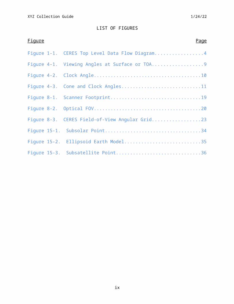
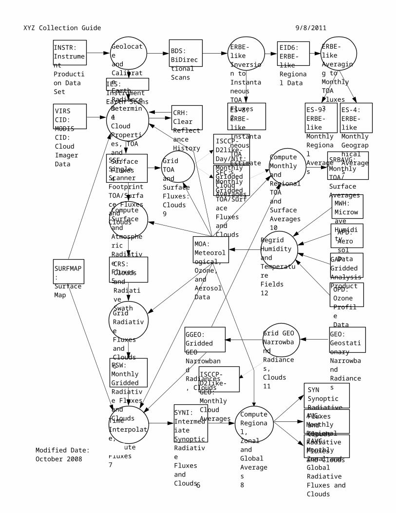
The CERES Data Management System (DMS) is a software management and processing system which processes CERES instrument measurements and associated engineering data to produce archival science and other data products. The DMS is executed at the LaRC ASDC, which is also responsible for distributing the data products. A high-level view of the CERES DMS is illustrated by the CERES Top Level Data Flow Diagram shown in Figure 1-1.

Circles in the diagram represent algorithm processes called subsystems, which are a logical collection of algorithms that together convert input products into output products. Boxes represent archival products. Two parallel lines represent data stores which are designated as nonarchival or temporary data products. Boxes or data stores with arrows entering a circle are

2


input sources for the subsystem, while boxes or data stores with arrows exiting the circles are output products.

1.4 Summary of Parameters[Product Specific Information – could be table of parameters here instead of in Section 4]

1.5 Discussion[Product Specific Information]

1.6 Related CollectionsSee the CERES Data Products Catalog (Reference 1) for a complete product listing.

3

Grid TOAand SurfaceFluxes:Clouds9

ERBE-likeAveraging toMonthly TOAFluxes3

Grid GEONarrowbandRadiances,Clouds11

GEO:GeostationaryNarrowbandRadiances

TimeInterpolate,ComputeFluxes7

Grid RadiativeFluxes andClouds6

MOA:Meteorological,Ozone, andAerosol Data

ES-8:ERBE-likeInstantaneousTOA Estimates

ERBE-likeInversion toInstantaneousTOA Fluxes2

RegridHumidityandTemperatureFields12

BDS:BiDirectionalScans

SRBAVG:Monthly TOA/Surface Averages

SYNI:IntermediateSynopticRadiativeFluxes and Clouds

ComputeMonthly andRegional TOAand SurfaceAverages10

DetermineCloudProperties, TOAand Surface Fluxes4

Geolocateand CalibrateEarthRadiances1

SSF: SingleScanner Footprint TOA/Surface Fluxes and Clouds

CRS: Cloudsand RadiativeSwath

VIRS CID:MODIS CID:CloudImager Data

SURFMAP:SurfaceMap

INSTR:InstrumentProduction Data Set

EID6:ERBE-like Regional Data

AVG:Monthly RegionalRadiative Fluxesand Clouds

ZAVG:Monthly Zonal and Global Radiative Fluxes and Clouds

ComputeRegional,Zonal andGlobalAverages8

GGEO:Gridded GEONarrowbandRadiances, CloudsFSW:

Monthly Gridded Radiative Fluxes andClouds

IES: InstrumentEarth Scans

CRH:ClearReflectanceHistory

GAP:Gridded Analysis ProductOPD:OzoneProfileData

MWH:MicrowaveHumidityAPD:AerosolData

SFC: MonthlyGridded TOA/SurfaceFluxes and Clouds

ES-9:ERBE-likeMonthly Regional Averages

ES-4:ERBE-likeMonthly Geographical Averages

ComputeSurface andAtmosphericRadiativeFluxes5

SYNSynopticRadiativeFluxes and Clouds

ISCCP-D2like-Day/Nit:Monthly Gridded Cloud Averages

ISCCP-D2like-GEO:Monthly Cloud Averages

Modified Date: October 2008


Figure 1-1. CERES Top Level Data Flow Diagram4


2.0 InvestigatorsDr. Bruce A. Wielicki, CERES Principal InvestigatorE-mail: [email protected]: (757) 864-5683FAX: (757) 864-7996Mail Stop 420Atmospheric Sciences CompetencyBuilding 125021 Langley BoulevardNASA Langley Research CenterHampton, VA 23681-2199

2.1 Title of InvestigationSubsystem Name [Subsystem #]e.g.,. Geolocate and Calibrate Earth Radiances (Subsystem 1.0)

2.2 Contact InformationWorking Group Chair Name, Subsystem X Working Group ChairMail Stop 420Atmospheric Sciences Research21 Langley BoulevardNASA Langley Research CenterHampton, Virginia 23681-2199Telephone: (757) 864-xxxxFAX: (757) 864-7996E-mail: [email protected]

5


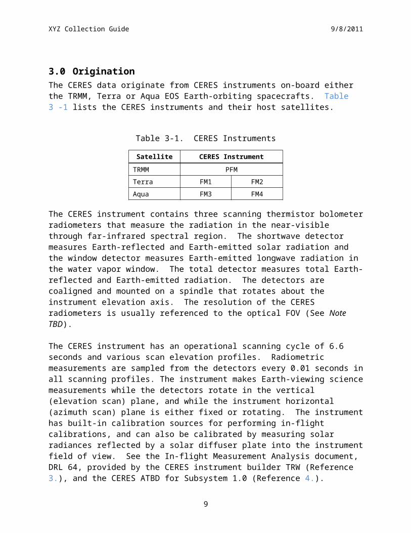
3.0 OriginationThe CERES data originate from CERES instruments on-board either the TRMM, Terra or Aqua EOS Earth-orbiting spacecrafts. Table 3-1 lists the CERES instruments and their host satellites.

Table 3-1. CERES Instruments

Satellite CERES InstrumentTRMM PFMTerra FM1 FM2Aqua FM3 FM4

The CERES instrument contains three scanning thermistor bolometer radiometers that measure the radiation in the near-visible through far-infrared spectral region. The shortwave detector measures Earth-reflected and Earth-emitted solar radiation and the window detector measures Earth-emitted longwave radiation in the water vapor window. The total detector measures total Earth-reflected and Earth-emitted radiation. The detectors are coaligned and mounted on a spindle that rotates about the instrument elevation axis. The resolution of the CERES radiometers is usually referenced to the optical FOV (See Note TBD).

The CERES instrument has an operational scanning cycle of 6.6 seconds and various scan elevation profiles. Radiometric measurements are sampled from the detectors every 0.01 seconds in all scanning profiles. The instrument makes Earth-viewing science measurements while the detectors rotate in the vertical (elevation scan) plane, and while the instrument horizontal (azimuth scan) plane is either fixed or rotating. The instrument has built-in calibration sources for performing in-flight calibrations, and can also be calibrated by measuring solar radiances reflected by a solar diffuser plate into the instrument field of view. See the In-flight Measurement Analysis document, DRL 64, provided by the CERES instrument builder TRW (Reference 3), and the CERES ATBD for Subsystem 1.0 (Reference 4).

6


4.0 Data Description

4.1 Spatial Characteristics

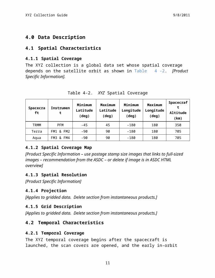
4.1.1 Spatial CoverageThe XYZ collection is a global data set whose spatial coverage depends on the satellite orbit as shown in Table 4-2. [Product Specific Information].

Table 4-2. XYZ Spatial Coverage

Spacecraft InstrumentMinimumLatitude

(deg)

MaximumLatitude

(deg)

MinimumLongitude

(deg)

MaximumLongitude

(deg)

SpacecraftAltitude

(km)TRMM PFM -45 45 -180 180 350Terra FM1 & FM2 -90 90 -180 180 705Aqua FM3 & FM4 -90 90 -180 180 705

4.1.2 Spatial Coverage Map[Product Specific Information – use postage stamp size images that links to full-sized images – recommendation from the ASDC – or delete if image is in ASDC HTML overview]

4.1.3 Spatial Resolution[Product Specific Information]

4.1.4 Projection[Applies to gridded data. Delete section from instantaneous products.]

4.1.5 Grid Description[Applies to gridded data. Delete section from instantaneous products.]

4.2 Temporal Characteristics

4.2.1 Temporal CoverageThe XYZ temporal coverage begins after the spacecraft is launched, the scan covers are opened, and the early in-orbit calibration check-out is completed (see ).

7


Table 4-3. XYZ Temporal Coverage

Spacecraft Instrument Launch Date Start Date End Date

TRMM PFM 11/27/1997 12/27/19978/31/1998Error:

Reference source not

found

Terra FM1 & FM2 12/18/1999 02/24/2000 TBDAqua FM3 & FM4 05/05/2002 06/19/2002 TBD

a. The CERES instrument on TRMM has operated only occasionally since 9/1/98 due to a power converter anomaly.

[Product Specific Information]

4.2.2 Temporal Resolution[Product Specific Information]

4.3 Data Characteristics[Product Specific Information]

4.3.1 Parameter/Variable[Product Specific Information] Table of parameters, units, ranges, …- similar to Table in Data Products Catalog. Describe the table and any hyperlinking. The XYZ metadata are listed in Appendix A.

4.3.2 Variable Description/Definition[Product Specific Information - a detailed definition of each parameter. If the parameter is copied from a product produced by a previous subsystem, the producing subsystem will define the parameter. All users must have chance to review and approve the definitions. A parameter will be defined only once and will be pulled into each relevant document - the following parameters are examples from the BDS Guide, in which the parameters are grouped into 3 major divisions - 2 of those are shown as examples.]

4.3.2.1 Science Parameter DescriptionsThe CERES science parameters are computed using the geodetic coordinate system. However, several parameters are computed in the geocentric coordinate system, and will specifically include the term "geocentric" in the parameter name. The geocentric parameters are used by the ERBElike Subsystems since ERBE products are archived in the geocentric coordinate system.

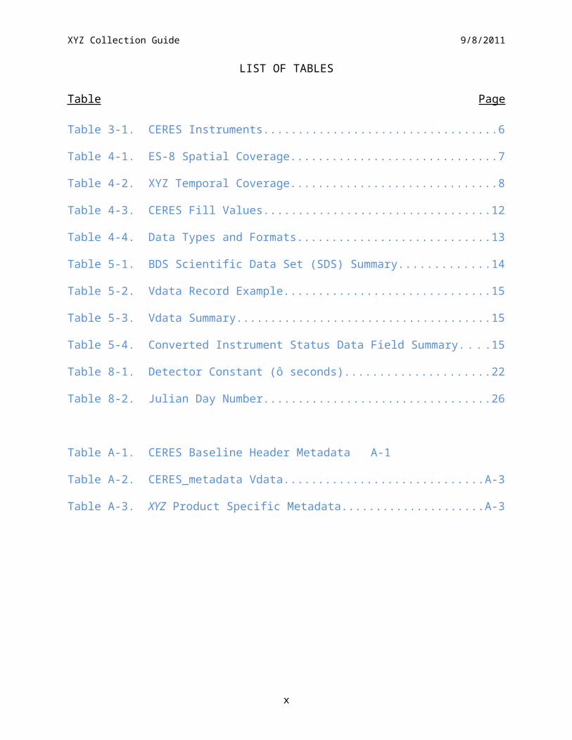
SCI-1 CERES Relative Azimuth at SurfaceThis parameter is the geodetic azimuth angle (See Figure 4-2) at the Earth point (See Term-4) of the satellite relative to the solar plane. (deg) [0 .. 360] {Section 5.2.1 Scientific Data Sets (SDS)}

The relative azimuth is measured clockwise in the plane normal to the geodetic zenith (See Term-9) so that the relative azimuth of the Sun is always 180o. The solar plane is the plane

8

Sun

Zenith (geodetic or geocentric)

Earth Point orTOA Point

Satellite

SolarPlane

ForwardScatter

Planenormalto Zenith


which contains the geodetic zenith vector and a vector from the Earth point to the Sun. If the Earth point is north of the geodetic subsolar point (See Term-8) on the same meridian, then an azimuth of 90o would imply the satellite is east of the Earth point.

Figure 4-2. Viewing Angles at Surface or TOA

SCI-2 CERES Relative Azimuth at TOA - GeocentricThis parameter is the geocentric azimuth angle (See Figure 4-2) at the TOA point (See Term-14) of the satellite relative to the solar plane. (deg) [0 .. 360] {Section 5.2.1 Scientific Data Sets (SDS)}

The relative azimuth is measured clockwise in the plane normal to the geocentric zenith (See Term-7) so that the relative azimuth of the Sun is always 180o. The solar plane is the plane which contains the geocentric zenith vector and a vector from the TOA point to the Sun. If the TOA point is north of the geocentric subsolar point (See Term-6) on the same meridian, then an azimuth of 90o would imply the satellite is east of the target point.

SCI-3 CERES Solar Zenith at SurfaceThis parameter is the geodetic zenith angle o (See Figure 4-2) at the Earth point (See Term-4) of the Sun. (deg) [0 .. 180] {Section 5.2.1 Scientific Data Sets (SDS)}

The geodetic solar zenith is the angle between the geodetic zenith (See Term-9) vector and a vector from the Earth point to the Sun.

SCI-4 CERES Solar Zenith at TOA - GeocentricThis parameter is the geocentric zenith angle o (See Figure 4-2) at the TOA point (See Term-14) of the Sun. (deg) [0 .. 180] {Section 5.2.1 Scientific Data Sets (SDS)}

The geocentric solar zenith is the angle between the geocentric zenith (See Term-7) vector and a vector from the TOA point to the Sun.

9

Angularmomentumvector

Greenw

ich

Earth Equator

Earth pointat surface

Satellite

InertialVelocity

=clock

Radius tosatellite

Z

X

Y


SCI-5 CERES Viewing Zenith at SurfaceThis parameter is the geodetic angle (See Figure 4-2) at the Earth point (See Term-4) to the satellite. (deg) [0 .. 90] {Section 5.2.1 Scientific Data Sets (SDS)}

The geodetic viewing zenith is the angle between the geodetic zenith (See Term-7) vector and a vector from the Earth point to the satellite.

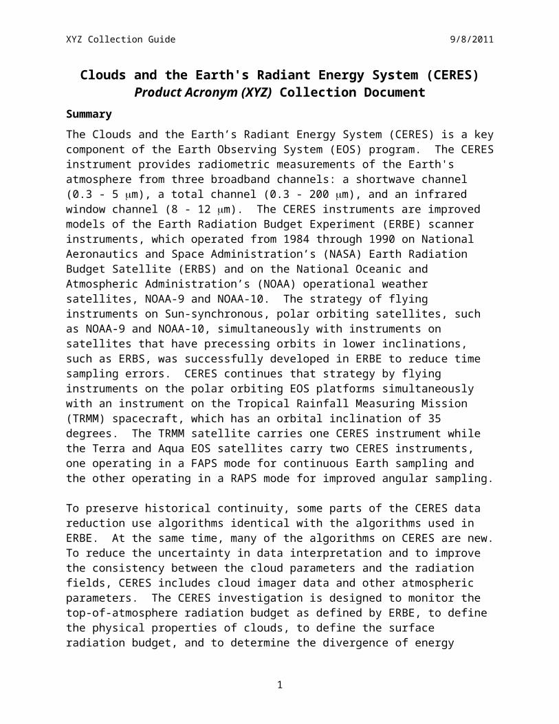
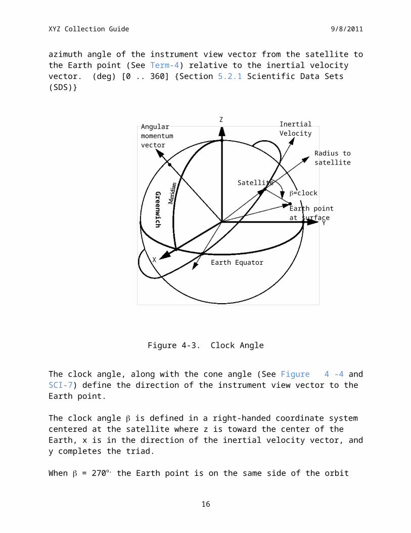
SCI-6 Clock Angle of CERES FOV at Satellite wrt Inertial VelocityThe clock angle (See Figure 4-3 and Figure 4-4) is the azimuth angle of the instrument view vector from the satellite to the Earth point (See Term-4) relative to the inertial velocity vector. (deg) [0 .. 360] {Section 5.2.1 Scientific Data Sets (SDS)}

Figure 4-3. Clock Angle

The clock angle, along with the cone angle (See Figure 4-4 and SCI-7) define the direction of the instrument view vector to the Earth point.

The clock angle is defined in a right-handed coordinate system centered at the satellite where z

10

Earthpoint

Nadir

Center of Earth

= clocksatellite

= cone


is toward the center of the Earth, x is in the direction of the inertial velocity vector, and y completes the triad.

When = 270o, the Earth point is on the same side of the orbit as the orbital angular momentum vector (See Figure 4-3). When = 0o, the Earth point is directly ahead of the satellite.

The toolkit call (See Reference 5) PGS_CSC_SCtoORB transforms the instrument view vector in spacecraft coordinates to (x,y,z) orbital coordinates and the clock angle is defined by

x /d=cos βand

y /d=sin βand

d=√x2+ y2

SCI-7 Cone Angle of CERES FOV at SatelliteThe cone angle (See Figure 4-4) is the angle between a vector from the satellite to the center of the Earth and the instrument view vector from the satellite to the Earth point (See Term-2). (deg) [0 .. 90] {Section 5.2.1 Scientific Data Sets (SDS)}

The cone angle, along with the clock angle, (See Figure 4-3 and SCI-6) define the direction of the instrument view vector to the Earth point.

The toolKit call (See Reference 5) PGS_CSC_SCtoORB transforms the instrument view vector in spacecraft coordinates to (x,y,z) orbital coordinates (See SCI-6) and the cone angle is defined by z=cos α .

Figure 4-4. Cone and Clock Angles

11


4.3.2.2 Instrument Parameter Descriptions[Bunch of parameters in alphabetical ordered related to the instrument or housekeeping parameters.]

INS-1 Elevation Offset CorrectionThis parameter indicates an internal count adjustment to compensate for the encoder position to actual gimbal position misalignment. This value will reflect the internal default value or the last update by the Set_Elevation_Offset_Correction command. The converted value is computed using DRL-64 (Reference 2) Algorithm Linear Coefficients. This value needs to be treated as a signed integer data representation. The default nominal unsigned and signed integer offset values for each instrument, as specified in the flight codes, are shown in Table B-4. (deg) [0 .. 360] {Section 5.2.2.1 Converted Instrument Status Data}

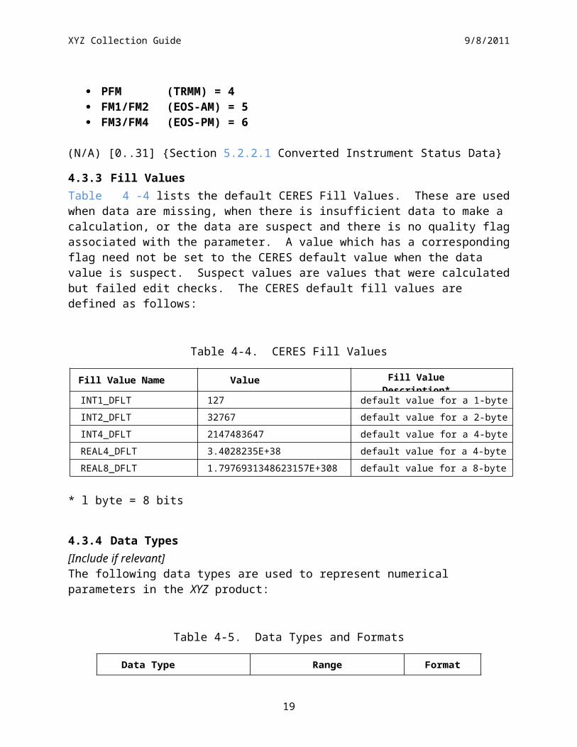
INS-2 Packet Data VersionThis parameter indicates the flight code version burned into the Instrument’s EPROMs. The default values for each of the instrument are shown below.

PFM (TRMM) = 4 FM1/FM2 (EOS-AM) = 5 FM3/FM4 (EOS-PM) = 6

(N/A) [0..31] {Section 5.2.2.1 Converted Instrument Status Data}

4.3.3 Fill ValuesTable 4-4 lists the default CERES Fill Values. These are used when data are missing, when there is insufficient data to make a calculation, or the data are suspect and there is no quality flag associated with the parameter. A value which has a corresponding flag need not be set to the CERES default value when the data value is suspect. Suspect values are values that were calculated but failed edit checks. The CERES default fill values are defined as follows:

Table 4-4. CERES Fill Values

Fill Value Name Value Fill Value Description*

INT1_DFLT 127 default value for a 1-byte integer



REAL4_DFLT 3.4028235E+38 default value for a 4-byte real

REAL8_DFLT 1.7976931348623157E+308 default value for a 8-byte real

* l byte = 8 bits

12


4.3.4 Data Types[Include if relevant]The following data types are used to represent numerical parameters in the XYZ product:

Table 4-5. Data Types and Formats

Data Type Range Format

Unsigned 8 Bit Integer 0..255 N/A

Signed 8 Bit Integer -127..127 N/A





32 Bit Float platform dependent 11.6

64 Bit Float platform dependent 13.8

4.4 Sample Data Record[Include 1 sample record with parameter labels or delete section.]

13


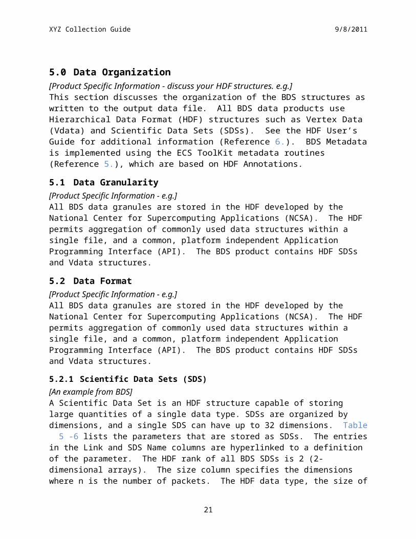
5.0 Data Organization[Product Specific Information - discuss your HDF structures. e.g.]This section discusses the organization of the BDS structures as written to the output data file. All BDS data products use Hierarchical Data Format (HDF) structures such as Vertex Data (Vdata) and Scientific Data Sets (SDSs). See the HDF User’s Guide for additional information (Reference 6). BDS Metadata is implemented using the ECS ToolKit metadata routines (Reference 5), which are based on HDF Annotations.

5.1 Data Granularity[Product Specific Information - e.g.]All BDS data granules are stored in the HDF developed by the National Center for Supercomputing Applications (NCSA). The HDF permits aggregation of commonly used data structures within a single file, and a common, platform independent Application Programming Interface (API). The BDS product contains HDF SDSs and Vdata structures.

5.2 Data Format[Product Specific Information - e.g.]All BDS data granules are stored in the HDF developed by the National Center for Supercomputing Applications (NCSA). The HDF permits aggregation of commonly used data structures within a single file, and a common, platform independent Application Programming Interface (API). The BDS product contains HDF SDSs and Vdata structures.

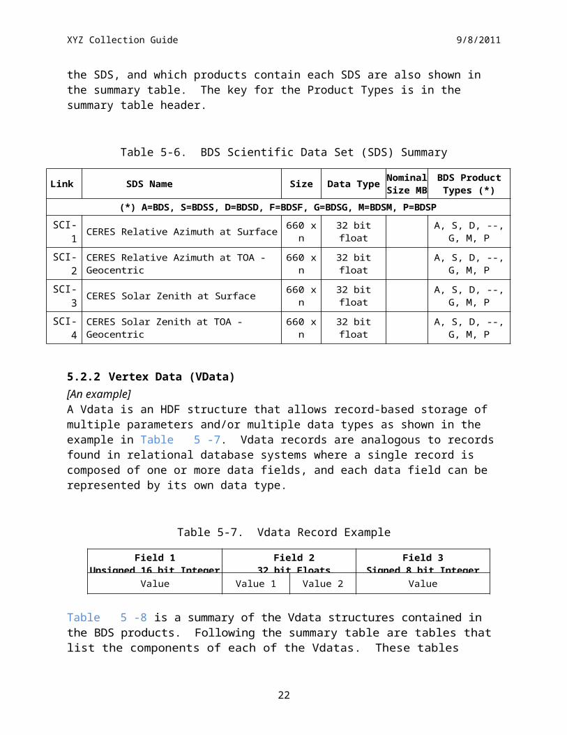
5.2.1 Scientific Data Sets (SDS)[An example from BDS]A Scientific Data Set is an HDF structure capable of storing large quantities of a single data type. SDSs are organized by dimensions, and a single SDS can have up to 32 dimensions. Table 5-6 lists the parameters that are stored as SDSs. The entries in the Link and SDS Name columns are hyperlinked to a definition of the parameter. The HDF rank of all BDS SDSs is 2 (2-dimensional arrays). The size column specifies the dimensions where n is the number of packets. The HDF data type, the size of the SDS, and which products contain each SDS are also shown in the summary table. The key for the Product Types is in the summary table header.

Table 5-6. BDS Scientific Data Set (SDS) Summary

Link SDS Name Size Data Type NominalSize MB

BDS ProductTypes (*)

(*) A=BDS, S=BDSS, D=BDSD, F=BDSF, G=BDSG, M=BDSM, P=BDSPSCI-1 CERES Relative Azimuth at Surface 660 x n 32 bit float A, S, D, --, G, M, P

SCI-2 CERES Relative Azimuth at TOA - Geocentric 660 x n 32 bit float A, S, D, --, G, M, P

SCI-3 CERES Solar Zenith at Surface 660 x n 32 bit float A, S, D, --, G, M, P

SCI-4 CERES Solar Zenith at TOA - Geocentric 660 x n 32 bit float A, S, D, --, G, M, P

14


5.2.2 Vertex Data (VData)[An example]A Vdata is an HDF structure that allows record-based storage of multiple parameters and/or multiple data types as shown in the example in Table 5-7. Vdata records are analogous to records found in relational database systems where a single record is composed of one or more data fields, and each data field can be represented by its own data type.

Table 5-7. Vdata Record Example

Field 1Unsigned 16 bit Integer

Field 232 bit Floats

Field 3Signed 8 bit Integer

Value Value 1 Value 2 Value

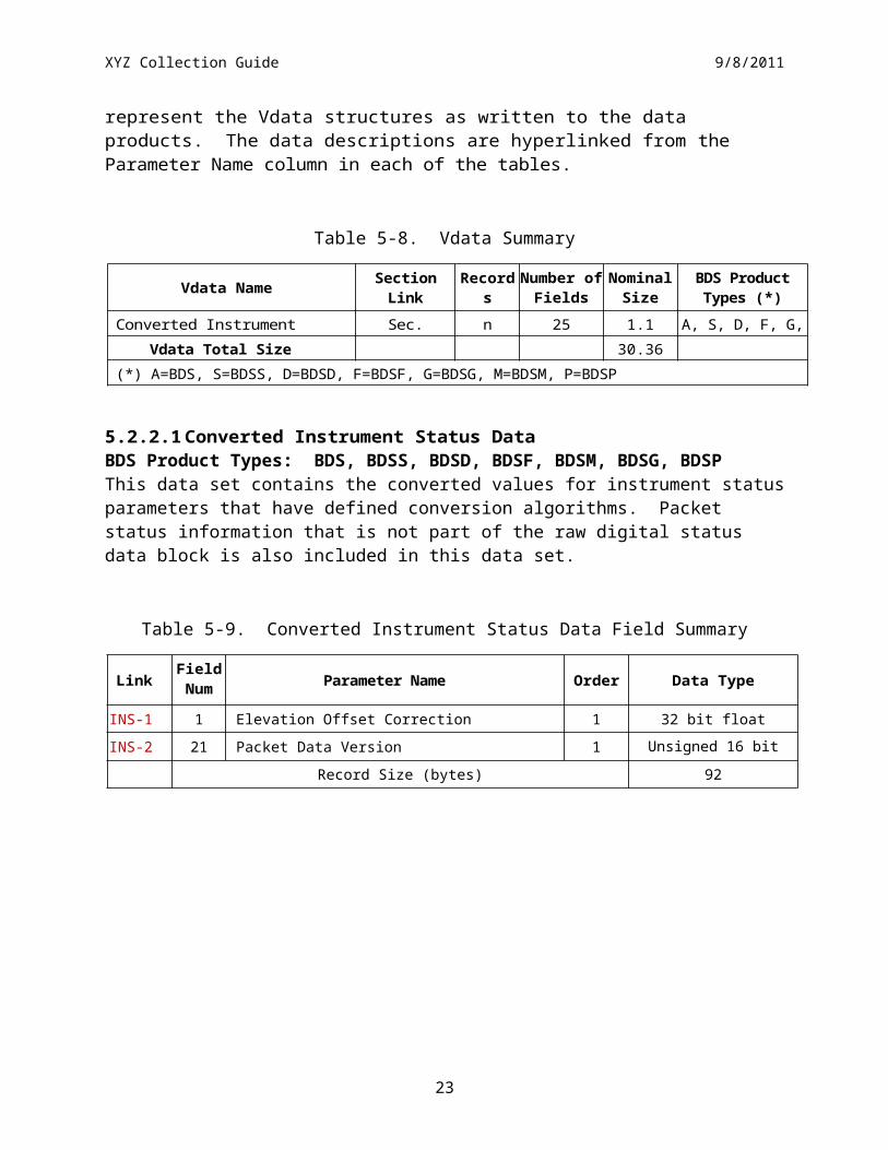
Table 5-8 is a summary of the Vdata structures contained in the BDS products. Following the summary table are tables that list the components of each of the Vdatas. These tables represent the Vdata structures as written to the data products. The data descriptions are hyperlinked from the Parameter Name column in each of the tables.

Table 5-8. Vdata Summary

Vdata Name Section Link RecordsNumber of

FieldsNominalSize (MB)

BDS Product Types (*)

Converted Instrument Status Data Sec. 5.2.2.1 n 25 1.1 A, S, D, F, G, M, P

Vdata Total Size 30.36

(*) A=BDS, S=BDSS, D=BDSD, F=BDSF, G=BDSG, M=BDSM, P=BDSP

5.2.2.1 Converted Instrument Status DataBDS Product Types: BDS, BDSS, BDSD, BDSF, BDSM, BDSG, BDSPThis data set contains the converted values for instrument status parameters that have defined conversion algorithms. Packet status information that is not part of the raw digital status data block is also included in this data set.

Table 5-9. Converted Instrument Status Data Field Summary

LinkFieldNum Parameter Name Order Data Type

INS-1 1 Elevation Offset Correction 1 32 bit float

INS-2 21 Packet Data Version 1 Unsigned 16 bit integer

15


Record Size (bytes) 92

16


6.0 Theory of Measurements and Data Manipulations

6.1 Theory of MeasurementsSee Reference 3 for the basic theory of measurements.

6.2 Data Processing Sequence[Product Specific Information]For detailed information see the Subsystem Architectural Design Document. (Reference 7)

6.3 Special Corrections/AdjustmentsAlgorithms not discussed in the ATBD are discussed in this section.

17


7.0 ErrorsSee CERES ATBD Subsystem Number. (Reference 4)[may wish to include high level accuracy goals]

7.1 Quality AssessmentQuality Assessment (QA) activities are performed at the Science Computing Facility (SCF) by the Data Management Team. Processing reports containing statistics and processing results are examined for anomalies. If the reports show anomalies, data visualization tools are used to examine those products in greater detail to begin the anomaly investigation. (See the QA flag description for this product.)

7.2 Data Validation by SourceSee Subsystem Subsystem Number Validation Document. (Reference 8) for details on the data validation plans.

18


8.0 Notes

Note-1 Field-of-View (FOV)

Field-of-View and footprint are synonymous. The CERES FOV is determined by its PSF (See Note-1 and Term-1) which is a two-dimensional, bell-shaped function that defines the CERES instrument response to the viewed radiation field.

The resolution of the CERES radiometers is usually referenced to the optical FOV which is 1.3o in the along-track direction and 2.6o in the cross-track direction. For example, on TRMM with a satellite altitude of 350 km, the optical FOV at nadir is 8 × 16 km which is frequently referred to as an equivalent circle with a 10 km diameter, or simply as 10 km resolution. On EOS-AM with a satellite altitude of 705 km, the optical FOV at nadir is 16 × 32 km or 20 km resolution.

The CERES FOV or footprint size is referenced to an oval area that represents approximately 95% of the PSF response (See Note-2 and Term-1) for numerical representation of FOV). Since the PSF is defined in angular space at the instrument, the CERES FOV is a constant in angular space, but grows in surface area from a minimum at nadir to a larger area at shallow viewing angles (See SCI-7). For TRMM, the length and width of this oval at nadir is 19 × 15 km and grows to 138 × 38 km at a viewing zenith angle (See SCI-7) of 70o. For EOS-AM/PM, the length and width at nadir is 38 × 31 km and grows to 253 × 70 km at a viewing zenith angle of 70o.

19


Note-2 CERES Point Spread Function

Note-2.1 CERES Point Spread Function

The CERES scanning radiometer is an evolutionary development of the ERBE scanning radiometer. It is desired to increase the resolution as much as possible, using a thermistor bolometer as the detector. As the resolution is increased, the sampling rate must increase to achieve spatial coverage. When the sampling rate becomes comparable to the response time of the detector, the effect of the time response of the detector on the PSF must be considered. Also, the signal is usually filtered electronically prior to sampling in order to attenuate electronic noises and to remove high frequency components of the signal which would cause aliasing errors. The time response of the filter, together with that of the detector causes a lag in the output relative to the input radiance. This time lag causes the centroid of the PSF to be displaced from the centroid of the optical FOV. Thus, the signal as sampled comes not only from where the radiometer is pointed, but includes a “memory” of the input from where it had been looking. Another effect of the time response is to broaden the PSF, which will reduce the resolution of the measurement, increase blurring errors, and decrease aliasing errors.

Note-2.2 Geometry of the Point Spread Function

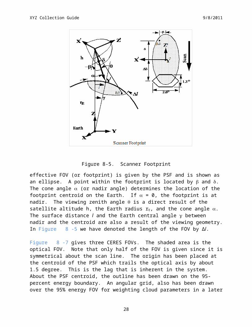
The scanner footprint geometry is given in Figure 8-5. The optical FOV is a truncated diamond (or hexagon) and is 1.3o in the along-scan direction and 2.6o in the across-scan direction. The

Figure 8-5. Scanner Footprint

20

(a,0)(-a,0)

(a,a)

(0,2a)

a=0.65

PSF=0

PSF≠0

Scan Direction


effective FOV (or footprint) is given by the PSF and is shown as an ellipse. A point within the footprint is located by and . The cone angle (or nadir angle) determines the location of the footprint centroid on the Earth. If = 0, the footprint is at nadir. The viewing zenith angle is a direct result of the satellite altitude h, the Earth radius rE, and the cone angle . The surface distance l and the Earth central angle between nadir and the centroid are also a result of the viewing geometry. In Figure 8-5 we have denoted the length of the FOV by Δl.

Figure 8-7 gives three CERES FOVs. The shaded area is the optical FOV. Note that only half of the FOV is given since it is symmetrical about the scan line. The origin has been placed at the centroid of the PSF which trails the optical axis by about 1.5 degree. This is the lag that is inherent in the system. About the PSF centroid, the outline has been drawn on the 95-percent energy boundary. An angular grid, also has been drawn over the 95% energy FOV for weighting cloud parameters in a later process. All of the pertinent dimensions are given.

Note-2.3 Analytic form of the Point Spread Function

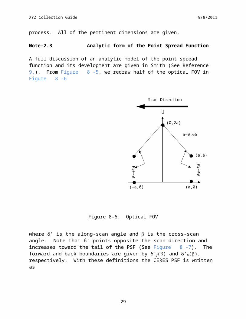
A full discussion of an analytic model of the point spread function and its development are given in Smith (See Reference 9). From Figure 8-5, we redraw half of the optical FOV in Figure 8-6

Figure 8-6. Optical FOV

where δ' is the along-scan angle and is the cross-scan angle. Note that δ' points opposite the scan direction and increases toward the tail of the PSF (See Figure 8-7). The forward and

21


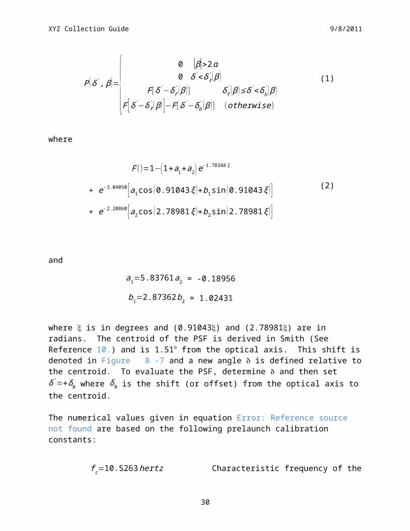
back boundaries are given by δ'f() and δ'b(), respectively. With these definitions the CERES PSF is written as

P (δ ' , β )={ 0 |β|>2α0 δ'<δ f

' ( β )F [δ'−δ f

' ( β )] δ f' (β ) ≤ δ'<δ b

' (β )F [δ '−δ f

' ( β ) ]−F [δ'−δb' ( β )] (otherwise)

(1)

where

F ()=1−(1+a1+a2 ) e−1.78348ξ

+ e−3.04050 [a1cos (0.91043 ξ )+b1 sin (0.91043 ξ ) ]

+ e−2.20860 [a2cos (2.78981 ξ )+b2 sin (2.78981ξ ) ]

(2)

and

a1=5.83761 a2 = -0.18956

b1=2.87362b2 = 1.02431

where is in degrees and (0.91043) and (2.78981) are in radians. The centroid of the PSF is derived in Smith (See Reference 10) and is 1.51o from the optical axis. This shift is denoted in Figure 8-7 and a new angle is defined relative to the centroid. To evaluate the PSF, determine and then set δ '=+δ 0 where δ 0 is the shift (or offset) from the optical axis to the centroid.

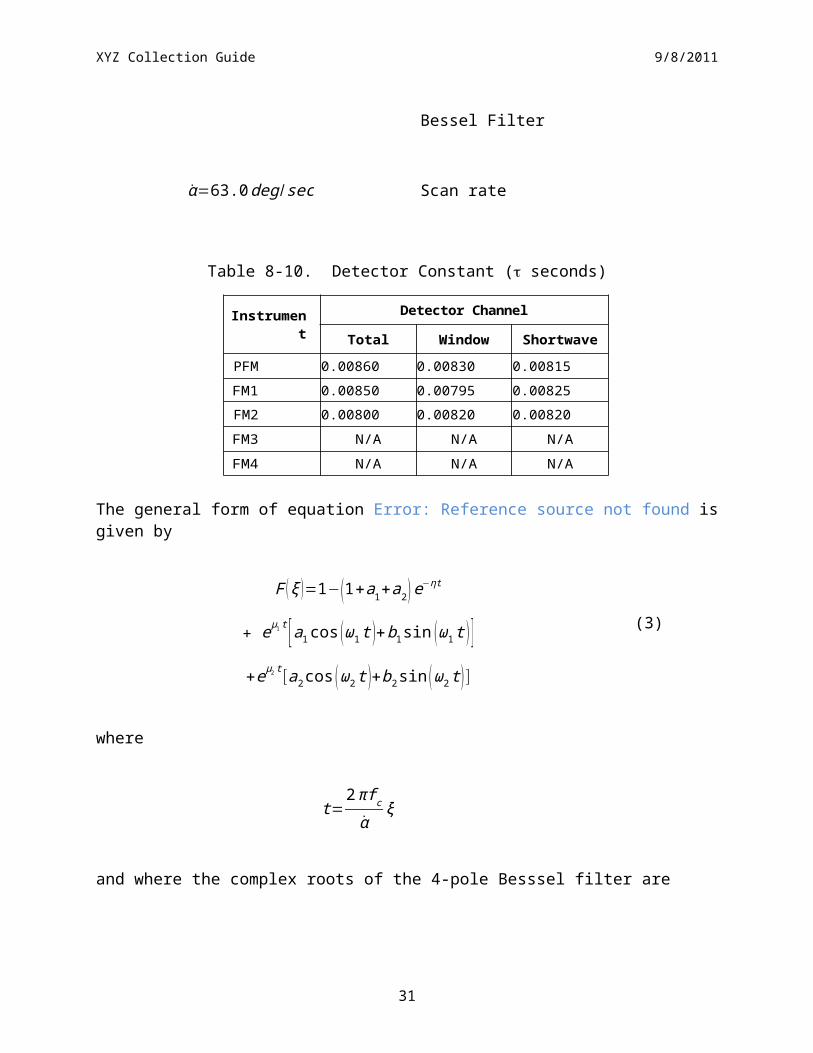
The numerical values given in equation Error: Reference source not found are based on the following prelaunch calibration constants:

f c=10.5263 hertz Characteristic frequency of the Bessel Filter

α̇=63.0deg /sec Scan rate

22


Table 8-10. Detector Constant ( seconds)

InstrumentDetector Channel

Total Window Shortwave

PFM 0.00860 0.00830 0.00815

FM1 0.00850 0.00795 0.00825

FM2 0.00800 0.00820 0.00820

FM3 N/A N/A N/A

FM4 N/A N/A N/A

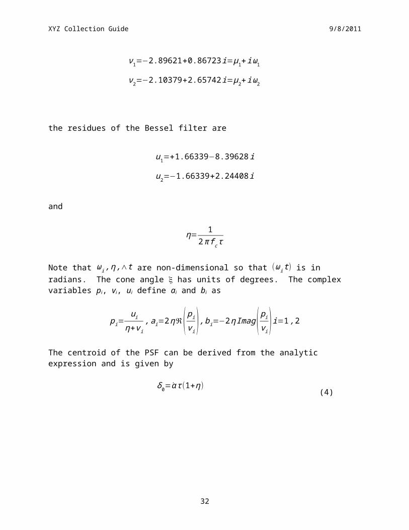
The general form of equation Error: Reference source not found is given by

F (ξ )=1−(1+a1+a2 ) e−ηt

+ eμ1 t [ a1cos (ω1 t )+b1 sin ( ω1 t ) ]

+eμ 2t [a2 cos (ω2t )+b2 sin (ω2t )]

(3)

where

t=2πf c

α̇ξ

and where the complex roots of the 4-pole Besssel filter are

ν1=−2.89621+0.86723 i=μ1+ iω1

ν2=−2.10379+2.65742i=μ2+ iω2

the residues of the Bessel filter are

u1=+1.66339−8.39628 i

u2=−1.66339+2.24408i

and

23


η= 12 π f c τ

Note that ωi , η ,∧t are non-dimensional so that (ωi t ) is in radians. The cone angle has units of degrees. The complex variables pi, vi, ui define ai and bi as

pi=ui

η+v i, ai=2 η ℜ( pi

v i) , bi=−2η Imag( pi

v i) i=1 ,2

The centroid of the PSF can be derived from the analytic expression and is given by

δ 0= α̇ τ (1+η)(4)

Figure 8-7. CERES Field-of-View Angular Grid

24


Note-3 Conversion of Julian Date to Calendar Date

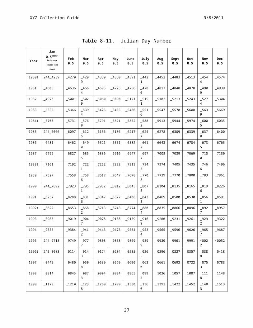
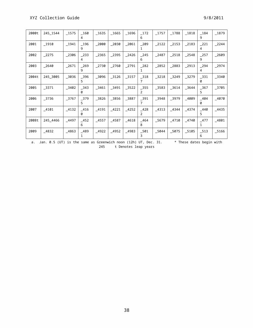
The Julian Date is a time system that has been adopted by astronomers and is used in many scientific experiments. The Julian Date or Julian Day is the number of mean solar days since 1200 hours (GMT/UT/UTC/Zulu) on Monday, 24 November 4714 BCE, based on the current Gregorian calendar, or more precisely, the Gregorian Proleptic calendar. In other words, Julian day number 0 (zero) was Monday, 24 November 4714 Before Current Era (BCE), 1200 hours (noon). A new Julian day starts when the mean Sun at noon crosses the Greenwich meridian. This differs from Universal Time (UT) or Greenwich Mean Solar Time by 12 hours since UT changes day at Greenwich midnight. Table 8-11 below provides Julian day numbers which relate Universal Time to Julian date.

Important facts related to the Gregorian calendar are:

a) There is no year zero; year -1 is immediately followed by year 1.

b) A leap year is any year which is divisible by 4, except for those centesimal years (years divisible by 100) which must also be divisible by 400 to be considered a leap year.

c) A leap year has 366 days, with the month of February containing 29 days.

d) Year -1 is defined as a leap year, thus being also defined as containing 366 days, and being divisible by 4, 100, and 400.

Information on history, calendars, and Julian day numbers can be found in Blackadar’s (Reference 10) “A Computer Almanac”, and on the WWW (Reference 11).

The Julian day whole number is followed by the fraction of the day that has elapsed since the preceding noon (1200 hours UTC). The Julian Date JDATE can be represented as:

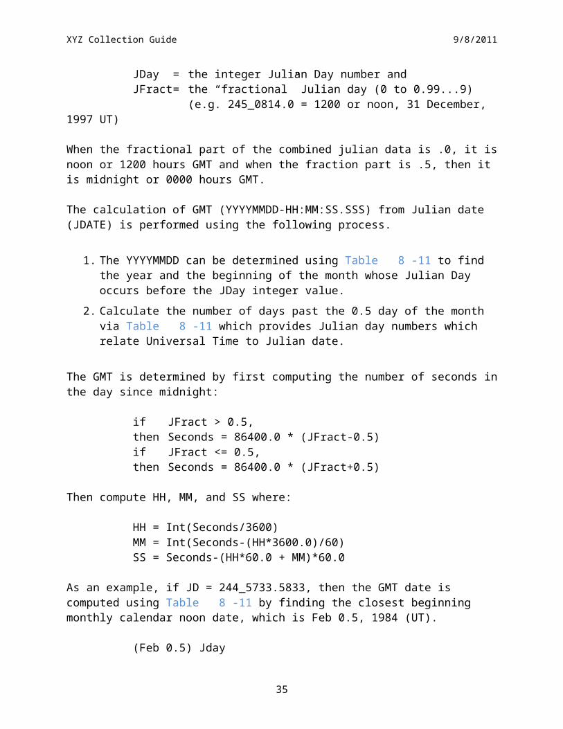
JDATE = JDay + JFract

where:JDay = the integer Julian Day number andJFract = the “fractional” Julian day (0 to 0.99...9)

(e.g. 245_0814.0 = 1200 or noon, 31 December, 1997 UT)

When the fractional part of the combined julian data is .0, it is noon or 1200 hours GMT and when the fraction part is .5, then it is midnight or 0000 hours GMT.

The calculation of GMT (YYYYMMDD-HH:MM:SS.SSS) from Julian date (JDATE) is performed using the following process.

1. The YYYYMMDD can be determined using Table 8-11 to find the year and the beginning of the month whose Julian Day occurs before the JDay integer value.

2. Calculate the number of days past the 0.5 day of the month via Table 8-11 which provides Julian day numbers which relate Universal Time to Julian date.

25


The GMT is determined by first computing the number of seconds in the day since midnight:

if JFract > 0.5,then Seconds = 86400.0 * (JFract-0.5)if JFract <= 0.5,then Seconds = 86400.0 * (JFract+0.5)

Then compute HH, MM, and SS where:

HH = Int(Seconds/3600)MM = Int(Seconds-(HH*3600.0)/60)SS = Seconds-(HH*60.0 + MM)*60.0

As an example, if JD = 244_5733.5833, then the GMT date is computed using Table 8-11 by finding the closest beginning monthly calendar noon date, which is Feb 0.5, 1984 (UT).

(Feb 0.5) Jday244 5731 < 244 5733.5833

JD = 244_5733.5833 is 2.5833 days past Feb 0.5, 1984 UT (i.e., past 1984 Jan 31d 12h 0m 0s) where 1984 Jan 31d 12h 0m 0ss = (244_5733-244_5731).

Beginning with the whole days portion of 2.5833 (i.e., 2), the GMT Date is 1984 Jan 31d 12h 0m 0s + 2 = 1984 Feb 2d 12h 0m 0s.

Next, since JFract (0.5833) is > 0.5, 12h is added to the GMT Date, yielding: 1984 Feb 2d 12h

0m 0s + 12h 0m 0s = 1984 Feb 3d 0h 0m 0s.

Finally, to get the GMT time and since JFract (0.5833) is > 0.5, the number of seconds = 86400 *(0.5833 -0.5) = 7197.12 yielding:

HH = 7197.12 / 3600 = 01.9992 = 01h

MM = 7197.12 - ((1*3600) / 60) = 59.952 = 59m

SS = 7197.12 - ((1*60) + 59)*60) = 57.12s

Therefore, the GMT Date corresponding to the Julian Date 244_5733.5833 = 1984 Feb 3d 1h 59m 57.12s, which is UT = 1984 Jan 31d 12h 0m 0s + 2.5833 days.

26


Table 8-11. Julian Day Number

Year

Jan0.5Error:

Reference source

not found

Feb 0.5

Mar 0.5

Apr 0.5

May 0.5

June 0.5

July 0.5

Aug 0.5

Sept 0.5

Oct 0.5

Nov 0.5

Dec 0.5

1980t 244_4239 _4270 _4299 _4330 _4360 _4391 _4421 _4452 _4483 _4513 _4544 _4574

1981 _4605 _4636 _4664 _4695 _4725 _4756 _4786 _4817 _4848 _4878 _4909 _4939

1982 _4970 _5001 _5029 _5060 _5090 _5121 _5151 _5182 _5213 _5243 _5274 _5304

1983 _5335 _5366 _5394 _5425 _5455 _5486 _5516 _5547 _5578 _5608 _5639 _5669

1984t _5700 _5731 _5760 _5791 _5821 _5852 _5882 _5913 _5944 _5974 _6005 _6035

1985 244_6066 _6097 _6125 _6156 _6186 _6217 _6247 _6278 _6309 _6339 _6370 _6400

1986 _6431 _6462 _6490 _6521 _6551 _6582 _6612 _6643 _6674 _6704 _6735 _6765

1987 _6796 _6827 _6855 _6886 _6916 _6947 _6977 _7008 _7039 _7069 _7100 _7130

1988t _7161 _7192 _7221 _7252 _7282 _7313 _7343 _7374 _7405 _7435 _7466 _7496

1989 _7527 _7558 _7586 _7617 _7647 _7678 _7708 _7739 _7770 _7800 _7831 _7861

1990 244_7892 _7923 _7951 _7982 _8012 _8043 _8073 _8104 _8135 _8165 _8196 _8226

1991 _8257 _8288 _8316 _8347 _8377 _8408 _8438 _8469 _8500 _8530 _8561 _8591

1992t _8622 _8653 _8682 _8713 _8743 _8774 _8804 _8835 _8866 _8896 _8927 _8957

1993 _8988 _9019 _9047 _9078 _9108 _9139 _9169 _9200 _9231 _9261 _9292 _9322

1994 _9353 _9384 _9412 _9443 _9473 _9504 _9534 _9565 _9596 _9626 _9657 _9687

1995 244_9718 _9749 _9777 _9808 _9838 _9869 _9899 _9930 _9961 _9991 *0022 *0052

1996t 245_0083 _0114 _0143 _0174 _0204 _0235 _0265 _0296 _0327 _0357 _0388 _0418

1997 _0449 _0480 _0508 _0539 _0569 _0600 _0630 _0661 _0692 _0722 _0753 _0783

1998 _0814 _0845 _0873 _0904 _0934 _0965 _0995 _1026 _1057 _1087 _1118 _1148

1999 _1179 _1210 _1238 _1269 _1299 _1330 _1360 _1391 _1422 _1452 _1483 _1513

2000t 245_1544 _1575 _1604 _1635 _1665 _1696 _1726 _1757 _1788 _1818 _1849 _1879

2001 _1910 _1941 _1969 _2000 _2030 _2061 _2091 _2122 _2153 _2183 _2214 _2244

2002 _2275 _2306 _2334 _2365 _2395 _2426 _2456 _2487 _2518 _2548 _2579 _2609

2003 _2640 _2671 _2699 _2730 _2760 _2791 _2821 _2852 _2883 _2913 _2944 _2974

2004t 245_3005 _3036 _3965 _3096 _3126 _3157 _3187 _3218 _3249 _3279 _3310 _3340

2005 _3371 _3402 _3430 _3461 _3491 _3522 _3552 _3583 _3614 _3644 _3675 _3705

2006 _3736 _3767 _3795 _3826 _3856 _3887 _3917 _3948 _3979 _4009 _4040 _4070

2007 _4101 _4132 _4160 _4191 _4221 _4252 _4282 _4313 _4344 _4374 _4405 _4435

2008t 245_4466 _4497 _4526 _4557 _4587 _4618 _4648 _5679 _4710 _4740 _4771 _4801

2009 _4832 _4863 _4891 _4922 _4952 _4983 _5013 _5044 _5075 _5105 _5136 _5166

a. Jan. 0.5 (UT) is the same as Greenwich noon (12h) UT, Dec. 31. * These dates begin with 245 t Denotes leap years

27


9.0 Application of the Data Set[Product Specific Information]

28


10.0 Future Modifications and PlansModifications to the XYZ product are driven by validation results and any EOS-AM related parameters. The ASDC provides users notification of changes.

29


11.0 Software DescriptionThere is a C/Fortran90 read program that interfaces with the HDF libraries and a README file available from the LaRC ASDC User Services. The program was designed to run on a Unix workstation and can be compiled with a C/Fortran90 compiler.

[Correct for fortran or C] {Pointer to ASDC read program}

30


12.0 Contact Data Center/Obtain DataEOSDIS Langley DAAC Telephone: (757) 864-8656USer and Data Service OfficeFAX: (757) 864-8807NASA Langley Research Center E-mail: [email protected] Mail Stop 157D URL: http://eosweb.larc.nasa.gov/ 2 South Wright StreetHampton, VA 23681-2199USA

31

http://eosweb.larc.nasa.gov/

mailto:E-mail:%20%[email protected]


13.0 Output Products and AvailabilitySeveral media types are supported by the Langley ASDC CERES Web Order Tool. Data can be downloaded from the Web or via FTP. Alternatively, data can be ordered on media tapes. The media tapes supported are 4mm 2Gb (90m), 8mm 2Gb (8200), 8mm 5Gb (8500), and 8mm 7Gb (8500c).

Data ordered via the Web or via FTP can be downloaded in either Uncompressed mode or in UNIX Compressed mode. Data written to media tape (in either Uncompressed mode or in UNIX Compressed mode) is in UNIX TAR format.

32


14.0 References1. Clouds and the Earth’s Radiant Energy System (CERES) Data Management System Data

Products Catalog Release 3, Version 0, April 1998 {URL = http://ceres.larc.nasa.gov/dpc_current.php}

2. TRW DRL 64, 55067.300.008E; In-flight Measurement Analysis (Rev. E), March 1997.

3. Clouds and the Earth’s Radiant Energy System (CERES) Algorithm Theoretical Basis Document, Instrument Geolocate and Calibrate Earth Radiances (Subsystem 1.0), Release 2.2, June 1997 {URL = http://ceres.larc.nasa.gov/atbd.php}.

4. Clouds and the Earth’s Radiant Energy System (CERES) Algorithm Theoretical Basis Document, Subsystem Name (Subsystem Number), Release 2.2, Month 1997 {URL = http://ceres.larc.nasa.gov/atbd.php}

5. Release B SCF ToolKit User's Guide for the ECS Project, June 1998.

6. HDF User's Guide, Version 4.0, February 1996 (from NCSA) {URL = http://eosweb/ HBDOCS/hdf.html }.

7. Subsystem Name (Subsystem Number) Draft Architectural Design Document Release 1.0, June 1996 {URL = http://ceres.larc.nasa.gov/sdd.php}.

8. Subsystem Validation Plan Name Release 1.1, March 1996 {URL = http://ceres.larc.nasa.gov/validation.php}

9. Smith, G. L., 1994, "Effects of time response on the point spread function of a scanning radiometer," Appl. Opt., Vol. 33, No. 30, 7031-7037.

10. Blackadar, Alfred, “A Computer Almanac,” Weatherwise, Vol 37, No 5, October 1984, p. 257-260.

11. Jefferys, William H. “Julian Day Numbers” {URL = http://quasar.as.utexas.edu/BillInfo/JulianDatesG.html}.

12. Software Bulletin "CERES Metadata Requirements for LaTIS", Revision 1, January 7, 1998 {URL = http://ceres.larc.nasa.gov/sw_bull.php}.

33

http://ceres.larc.nasa.gov/sw_bull.php

http://ceres.larc.nasa.gov/validation.php

http://ceres.larc.nasa.gov/sdd.php

http://eosweb/HBDOCS/hdf.html

http://ceres.larc.nasa.gov/atbd.php

http://ceres.larc.nasa.gov/atbd.php

http://ceres.larc.nasa.gov/dpc_current.php


15.0 Glossary of Terms

Term-1 CERES Point Spread Function

A Point Spread Function (PSF) is a two-dimensional bell-shaped function that defines the CERES instrument response to the viewed radiation field. Due to the response time, the radiometer responds to a larger FOV than the optical FOV and the resulting PSF centroid lags the optical FOV centroid by more than a degree of cone angle (See SCI-7) for normal scan rates (See Note-2).

Term-2 Earth Equator, Greenwich Meridian System

The Earth equator, Greenwich meridian system is an Earth-fixed, geocentric, rotating coordinate system with the X-axis in the equatorial plane through the Greenwich meridian, the Y-axis lies in the equatorial plane 90o to the east of the X-axis, and the Z-axis is toward the North Pole.

Term-3 Earth Surface

The surface of the Earth as defined by the WGS-84 Earth Model. The WGS-84 model of the

Earth surface is an ellipsoid x2

a2 + y2

a2 + z2

b2 =1 where a = 6378.1370 km and b = 6356.7523 km (See

Figure 15-9).

Term-4 Earth Point

The viewed point on the Earth surface (See Term-3), or the point at which the PSF centroid intersects the Earth surface.

Term-5 Field-of-View

The terms Field of View (FOV) and footprint are synonymous (See Note-1). The CERES FOV is determined by its PSF which is a two dimensional bell-shaped function that defines the CERES instrument response to the viewed radiation field.

The resolution of the CERES radiometers is usually referenced to the optical FOV and is 1.3o in the along-track direction and 2.6o in the cross-track direction. For TRMM with a satellite altitude of 350 km, the nadir optical FOV is 8 × 16 km which is frequently referred to as an equivalent circle with a 10 km diameter, or simply as 10 km resolution. For EOS-AM with a satellite altitude of 705 km, the optical FOV at nadir is 16 × 32 km or 20 km resolution.

The CERES footprint size is referenced as an oval area representing ~95% of the PSF response (See Note-1). Since the PSF is defined in instrument angular space, the CERES FOV is a constant in angular space, but grows in surface area from a minimum at nadir to a larger area at shallow viewing angles (See SCI-7). At nadir, this oval for TRMM is 19 × 15 km (EOS-AM is 38 × 31 km) and grows to 138 × 38 km (EOS-AM is 253 × 70 km) at a 70o viewing zenith angle.

34

Z

GeocentricSubsolarPoint

GeocentricSubsolarPoint

Ellipsoid

Surface Tangent

b

a

Sun

GeocentricZenith

XY

c

d

Z GeodeticZenith


The ToolKit routine PGS_CSC_GetFOV_Pixel returns the geodetic latitude and longitude of the intersection of the FOV centroid and the selected Model Surface. The returned longitudes are transformed from radians to degrees and then converted from to ±180o to 0o .. 360o. The returned geodetic latitudes are transformed from radians to degrees and then converted to geodetic colatitude using (90.0-latitude).

Term-6 Geocentric Subsolar Point

The point on a surface where the geocentric zenith (See Term-7) vector points toward the Sun (See Figure 15-8).

Term-7 Geocentric Zenith

A vector from the center of the Earth (See Figure 15-9) to the point of interest.

Term-8 Geodetic Subsolar Point

The point on a surface where the geodetic zenith (See Term-9) vector points toward the Sun (See Figure 15-8). Although the geocentric latitude c and the geodetic latitude d are equal, the geocentric subsolar point is different from the geodetic subsolar point.

Figure 15-8. Subsolar Point

The ToolKit routine PGS_CBP_Earth_CB_vector calculates the Earth-Centered Inertial (ECI) position vector from the Earth to the Sun. A second ToolKit routine, PGS_CSC_ECItoECR, transforms the position vector to the ECR or Earth equator, Greenwich meridian rectangular

35

Ellipsoid

GeodeticZenith Geocentric

Zenith

SurfaceTangent

a

b

Z

Y c d

r

X


coordinate system. From these coordinates, the geocentric colatitude and longitude of the Sun are calculated.

Term-9 Geodetic Zenith

The vector normal to an ellipsoid (See Figure 15-9) at a point on the surface. At a point on the

surface the geocentric latitude c and the geodetic latitude d are related by tanθc=b2

a2 .tanθd. We

can determine the radial distance r as a function of the geocentric latitude c by setting x = r cosc), y = 0, z = r sin(c) in the ellipsoidal model and solving for r or

r= ab

√a2sin2 θc+b2 cos2 θc

The semi-major axis (a) and the semi-minor axis (b) are defined by either the Earth Surface (See Term-3) or the TOA (See Term-13).

Figure 15-9. Ellipsoid Earth Model

Term-10 Julian Date

A continuous count of time in whole and fractional days elapsed at the Greenwich meridian since noon on January 1, 4714 BCE. (See Note-1)

Term-11 Subsatellite Point

36

Z

b

a

GeocentricSubsatellitePoint

GeocentricZenith

GeodeticZenith

SurfaceTangent

X

Ellipsoid

c dYGeocentricSubsatellitePoint

Satellite


The point on a surface below the satellite or the intersection point of a line dropped from the satellite through the surface (See Figure 15-10). The geocentric subsatellite point is on the radius vector to the center of the earth. The geodetic subsatellite point is on the geodetic zenith vector or the line dropped from the satellite is normal to the surface at the intersection point.

The ToolKit routine PGS_CSC_SubSatPoint returns the geodetic latitude and longitude of the subsatellite point. The returned longitudes are transformed from radians to degrees and then converted from to ±180o to 0o..360o. The returned latitudes are transformed from radians to degrees and then converted to colatitude using (90.0 - latitude).

Figure 15-10. Subsatellite Point

Term-12 Target Point

The point at which the PSF (See Term-1) centroid intersects the TOA (See Term-13).

Term-13 Top-of-the-Atmosphere (TOA)

The TOA is a surface approximately 30 km above the Earth surface (See Term-3). Specifically,

the TOA is an ellipsoid x2

a2 + y2

a2 + z2

b2 =1 where a = 6408.1370 km and b = 6386.651 km (See

Figure 15-9).

Term-14 TOA Point

37


The viewed point at the TOA, or the point at which the PSF centroid intersects the TOA (See Term-13).

38


16.0 List of AcronymsADM Angular Distribution ModelAPID Application IdentifierAPD Aerosol Profile DataATBD Algorithm Theoretical Basis DocumentAVG Monthly Regional Radiative Fluxes and CloudsAVHRR Advanced Very High Resolution RadiometerBCE Before Current EraBDS BiDirectional Scan (data product)CADM CERES Angular Distribution ModelCER CERESCERES Clouds and the Earth’s Radiant Energy SystemCID Cloud Imager Data (data product)CRH Clear Reflectance History (data product)CRS Clouds and Radiative Swath (data product)CW Cable WrapDAAC Distributed Active Archive CenterDAC Digital to Analog ConverterDAO Data Assimilation OfficeDAP Data Acquisition microProcessorDMA Direct Memory AccessDMS Data Management SystemECR Earth-Centered RotatingEDDB ERBE-Like Daily Database ProductEDOS EOS Data Operations SystemEOS Earth Observing SystemEOS-AM EOS Morning Crossing Mission (Renamed Terra)EOS-PM EOS Afternoon Crossing MissionEOSDIS Earth Observing System Data and Information SystemERBE Earth Radiation Budget ExperimentERBS Earth Radiation Budget SatelliteFAPS Fixed Azimuth Plane ScanFM Flight ModelFOV Field-of-View (See Term-5)FSW Monthly Single Satellite Fluxes and CloudsGAP Gridded Analysis ProductGB GigabyteGEO Geostationary Narrowband RadiancesGMS Geostationary Meteorological Satellite

39


GGEO Gridded Geostationary Narrowband RadiancesGOES Geostationary Operational Environmental SatelliteH HighHDF Hierarchical Data FormatIES Instrument Earth Scans (data product)IGBP International Geosphere Biosphere ProgrammeINSTR InstrumentISCCP International Satellite Cloud Climatology ProjectIWC Ice Water ContentLaRC Langley Research CenterLaTIS Langley TRMM Information SystemL LowLM Lower MiddleLW LongwaveLWC Liquid Water ContentMAM Mirror Attenuator MosaicMB MegabyteMETEOSAT Meteorological SatelliteMISR Multi-angle Imaging SpectroRadiometerMOA Meteorological, Ozone, and Aerosols (data product)MODIS Moderate Resolution Imaging SpectrometerMWH Microwave Humidity (data product)NASA National Aeronautics and Space AdministrationNOAA National Oceanic and Atmospheric AdministrationOPD Ozone Profile Data (data product)PFM Prototype Flight Model (on TRMM)PSA Product Specific AttributePSF Point Spread Function (See Term-1)QA Quality AssessmentRAPS Rotating Azimuth Plane ScanSARB Surface and Atmospheric Radiation BudgetSBUV-2 Solar Backscatter Ultraviolet/Version 2SDS Scientific Data SetSFC Hourly Gridded Single Satellite TOA/Surface Fluxes and Clouds (data

product)SPS Solar Presence SensorSRB Surface Radiation BudgetSRBAVG Surface Radiation Budget Average (data product)SS SubsystemSSF Single Satellite CERES Footprint TOA and Surface Fluxes, Clouds (data

product)

40


SSM/I Special Sensor Microwave/ImagerSURFMAP Surface MapSW ShortwaveSWICS Shortwave Internal Calibration SourceSYN Synoptic Radiative Fluxes and CloudsTBD To Be DeterminedTISA Time Interpolation and Spatial AveragingTMI TRMM Microwave ImagerTOA Top-of-the-Atmosphere (See Term-13)TOT TotalTRMM Tropical Rainfall Measuring MissionUM Upper MiddleURL Uniform Resource LocatorUT Universal TimeUTC Universal Time CodeVIRS Visible Infrared ScannerWN WindowZAVG Monthly Zonal and Global Average Radiative Fluxes and Clouds (data

product)

Unit DefinitionsUnits Definition

AU Astronomical Unitcm centimetercount count, countsday day, Julian datedeg degreedeg sec-1 degrees per seconddu Dobson unitsfraction fraction 0..1g kg-1 gram per kilogramg m-2 gram per square meterhhmmss hour, minute, secondhour hourhPa hectoPascalsin-oz inch-ounceK Kelvinkm kilometer, kilometers

41


Unit DefinitionsUnits Definition

km sec-1 kilometers per secondm metermA milliamp, milliampsmicron micrometer, micronmsec millisecondmW cm-2sr-1m-1 milliWatts per square centimeter per steradian per micronm sec-1 meter per secondN/A not applicable, none, unitless, dimensionlesspercent percent, percentage 0..100rad radiansec secondvolt volt, voltsW h m-2 Watt hour per square meterW2 m-4 square Watt per meter to the 4th W m-2 Watt per square meterW m-2sr-1 Watt per square meter per steradianW m-2sr-1m-1 Watt per square meter per steradian per micronoC degrees centigradem micrometer, micron

42


17.0 Document Information

17.1 Document Creation Date – February 1998

17.2 Document Review Date - July 1998

17.3 Document Revision DateMonth 1999 Comment

17.4 Document IDLD_007_010_001_00_00_0_yyyymmdd (Release Date) [get this from ASDC User Services]

17.5 CitationPlease provide a reference to the following paper when scientific results are published using the CERES XYZ TRMM data:

“Wielicki, B. A.; Barkstrom, B.R.; Harrison, E. F.; Lee III,R.B.; Smith, G.L.; and Cooper, J.E., 1996: Clouds and the Earth’s Radiant Energy System (CERES): An Earth Observing System Experiment, Bull. Amer. Meteor. Soc., 77, 853-868.”

When Langley Atmospheric Sciences Data Center (ASDC) data are used in a publication, the following acknowledgment is requested to be included:

“These data were obtained from the NASA Langley Research Center EOSDIS Distributed Active Archive Center.”

The Data Center at Langley requests two reprints of any published papers or reports which cite the use of data the Langley ASDC have distributed. This will help the ASDC to determine the use of data distributed, which is helpful in optimizing product development. It also helps the ASDC to keep product related references current.

17.6 Redistribution of DataTo assist the Langley ASDC in providing the best service to the scientific community, a notification is requested if these data are transmitted to other researchers.

17.7 Document CuratorThe Langley ASDC Science, User & Data Services Office.

43


Appendix A CERES Metadata

This section describes the metadata that are written to all CERES HDF products. Table A-1 describes the CERES Baseline Header Metadata that are written on both HDF and binary direct access output science data products. The parameters are written in HDF structures for CERES HDF output products and are written as 80-byte records for binary direct access output products. Some parameters may be written in multiple records. Table A-2 describes the CERES_metadata Vdata parameters which are a subset of the CERES Baseline Header Metadata and are also written to all CERES HDF output products. For details on CERES Metadata, see the CERES Software Bulletin “CERES Metadata Requirements for LaTIS” (Reference 12).

Table A-1 lists the item number, parameter name, units, range or allowable values, the data type, and the maximum number of elements. Note that there are two choices for parameters 22-25 and two choices for parameters 26-29. The choices depend on whether the product is described by a bounding rectangle or by a GRing. Abbreviations used in the Data Type field are defined as follows:

s = string date = yyyy-mm-ddF = float time = hh:mm:ss.xxxxxxZI = integer datetime = yyyy-mm-ddThh:mm:ss.xxxxxxZ

Table A-1. CERES Baseline Header Metadata

Item Parameter Name Units Range Data Type

No. of Elements

1 ShortName N/A N/A s(8) 1

2 VersionID N/A 0 .. 255 I3 1

3 CERPGEName N/A N/A s(20) 1

4 SamplingStrategy N/A CERES, TRMM-PFM-VIRS, AM1-FM1-MODIS, TBD

s(20) 1

5 ProductionStrategy N/A Edition, Campaign, Diagnostic- Case, PreFlight, TBD

s(20) 1

6 CERDataDateYear N/A 1997 .. 2050 s(4) 1

7 CERDataDateMonth N/A 1 .. 12 s(2) 1

8 CERDataDateDay N/A 1 .. 31 s(2) 1

9 CERHrOfMonth N/A 1 .. 744 s(3) 1

10 RangeBeginningDate N/A 1997-11-19 .. 2050-12-31 date 1

11 RangeBeginningTime N/A 00:00:00.000000Z ..24:00:00:000000Z

time 1

12 RangeEndingDate N/A 1997-11-19 .. 2050-12-31 date 1

13 RangeEndingTime N/A 00:00:00.000000Z ..24:00:00:000000Z

time 1

14 AssociatedPlatformShortName N/A TRMM, AM1, PM1, TBD s(20) 1 - 4

1


Table A-1. CERES Baseline Header Metadata

Item Parameter Name Units Range Data Type

No. of Elements

15 AssociatedInstrumentShortName N/A PFM, FM1, FM2, FM3, FM4, FM5, TBD

s(20) 1 - 4

16 LocalGranuleID N/A N/A s(80) 1

17 PGEVersion N/A N/A s(10) 1

18 CERProductionDateTime N/A N/A datetime 1

19 LocalVersionID N/A N/A s(60) 1

20 ProductGenerationLOC N/A SGI_xxx, TBD s(255) 1

21 NumberofRecords N/A 1 .. 9 999 999 999 I10 1

22 WestBoundingCoordinate deg -180.0 .. 180.0 F11.6 1

23 NorthBoundingCoordinate deg -90.0 .. 90.0 F11.6 1

24 EastBoundingCoordinate deg -180.0 .. 180.0 F11.6 1

25 SouthBoundingCoordinate deg -90.0 .. 90.0 F11.6 1

22 GRingPointLatitude deg -90.0 .. 90.0 F11.6 5

23 GRingPointLongitude deg -180.0 .. 180.0 F11.6 5

24 GRingPointSequenceNo N/A 0 .. 99999 I5 5

25 ExclusionGRingFlag N/A Y (= YES), N (= NO) s(1) 1

26 CERWestBoundingCoordinate deg 0.0 .. 360.0 F11.6 1

27 CERNorthBoundingCoordinate deg 0.0 .. 180.0 F11.6 1

28 CEREastBoundingCoordinate deg 0.0 .. 360.0 F11.6 1

29 CERSouthBoundingCoordinate deg 0.0 .. 180.0 F11.6 1

26 CERGRingPointLatitude deg 0.0 .. 180.0 F11.6 5

27 CERGRingPointLongitude deg 0.0 .. 360.0 F11.6 5

28 GRingPointSequenceNo N/A 0 .. 99999 I5 5

29 ExclusionGRingFlag N/A Y (= YES), N (= NO) s(1) 1

30 AutomaticQualityFlag N/A Passed, Failed, or Suspect s(64) 1

31 AutomaticQualityFlagExplanation N/A N/A s(255) 1

32 QAGranuleFilename N/A N/A s(255) 1

33 ValidationFilename N/A N/A s(255) 1

34 ImagerShortName N/A VIRS, MODIS, TBD s(20) 1

35 InputPointer N/A N/A s(255) 800

36 NumberInputFiles N/A 1 .. 9999 I4 1

Table A-2 describes the CERES_metadata Vdata parameters which are written to all CERES HDF output science products.

2


Table A-2. CERES_metadata Vdata

Item Parameter Name Units Range DataType

1 ShortName N/A s(32) 1

2 RangeBeginningDate 1997-11-19 .. 2050-12-31 s(32) 2

3 RangeBeginningTime 00:00:00.000000Z .. 24:00:00:000000Z s(32) 3

4 RangeEndingDate 1997-11-19 .. 2050-12-31 s(32) 4

5 RangeEndingTime 00:00:00.000000Z .. 24:00:00:000000Z s(32) 5

6 AutomaticQualityFlag Passed, Failed, or Suspect s(64) 6

7 AutomaticQualityFlagExplanation N/A s(256) 7

8 AssociatedPlatformShortName TRMM, EOS AM-1, EOS PM-1, TBD s(32) 8

9 AssociatedInstrumentShortName PFM, FM1, FM2, FM3, FM4, FM5, TBD s(32) 9

10 LocalGranuleID N/A s(96) 10

11 LocalVersionID N/A s(64) 11

12 CERProductionDateTime N/A s(32) 12

13 NumberofRecords 1 .. 9 999 999 999 4-byte Integer 13

14 ProductGenerationLOC SGI_xxx, TBD s(256) 14

The XYZ Product Specific Attribute (PSA) metadata are listed in Table A-3. The definitions that are nearly identical for several parameters are defined only once, even though individually distinct parameters exist as shown in the table below.

Table A-3. XYZ Product Specific Metadata

Item Parameter Name RangeDataType

15 Percent Total Channel Bad 0.0 .. 100.0 F11.6

16 Percent Window Channel Bad 0.0 .. 100.0 F11.6

17 Record Size (bytes) =nnn

PSA-1 Percent Total Channel BadPSA-2 Percent Window Channel BadThe percent of radiance samples that failed various edit checks and were then marked Bad during science processing.

3

Clouds and the Earth's Radiant Energy System€¦ · Web view · 2011-09-08The Clouds and the...

Documents

Transcript of Clouds and the Earth's Radiant Energy System€¦ · Web view · 2011-09-08The Clouds and the...