SANDIA REPORTSAND2001-1283Unlimited ReleasePrinted May 2001

Cloud to CAD

Arlo L. Ames

Prepared bySandia National LaboratoriesAlbuquerque, New Mexico 87185 and Livermore, California 94550

Sandia is a multiprogram laboratory operated by Sandia Corporation,a Lockheed Martin Company, for the United States Department ofEnergy under Contract DE-AC04-94AL85000.

Approved for public release; further dissemination unlimited.

Issued by Sandia National Laboratories, operated for the United States Departmentof Energy by Sandia Corporation.

NOTICE: This report was prepared as an account of work sponsored by an agencyof the United States Government. Neither the United States Government, nor anyagency thereof, nor any of their employees, nor any of their contractors,subcontractors, or their employees, make any warranty, express or implied, orassume any legal liability or responsibility for the accuracy, completeness, orusefulness of any information, apparatus, product, or process disclosed, or representthat its use would not infringe privately owned rights. Reference herein to anyspecific commercial product, process, or service by trade name, trademark,manufacturer, or otherwise, does not necessarily constitute or imply its endorsement,recommendation, or favoring by the United States Government, any agency thereof,or any of their contractors or subcontractors. The views and opinions expressedherein do not necessarily state or reflect those of the United States Government, anyagency thereof, or any of their contractors.

Printed in the United States of America. This report has been reproduced directlyfrom the best available copy.

Available to DOE and DOE contractors fromU.S. Department of EnergyOffice of Scientific and Technical InformationP.O. Box 62Oak Ridge, TN 37831

Telephone: (865)576-8401Facsimile: (865)576-5728E-Mail: reports@adonis.osti.govOnline ordering: http://www.doe.gov/bridge

Available to the public fromU.S. Department of CommerceNational Technical Information Service5285 Port Royal RdSpringfield, VA 22161

Telephone: (800)553-6847Facsimile: (703)605-6900E-Mail: orders@ntis.fedworld.govOnline order: http://www.ntis.gov/ordering.htm

SAND 2001-1283Unlimited ReleasePrinted May 2001

Cloud to CAD

Arlo L. AmesEngineering and Manufacturing SoftwareIntelligent Systems and Robotics Center

Sandia National LaboratoriesP. O. Box 5800

Albuquerque, NM 87185-1010

AbstractThis paper documents work performed to convert scanned range data to CAD solid modelrepresentation. The work successfully developed surface fitting algorithms for quadric surfaces(e.g. plane, cone, cylinder, and sphere), and a segmentation algorithm based entirely on surfacetype, rather than on a differential metric like Gaussian curvature. Extraction of all CAD-required parameters for quadric surface representation was completed. Approximate faceboundaries derived from the original point cloud were constructed. Work to extrapolatesurfaces, compute exact edges and solid connectivity was begun, but left incomplete due tofunding reductions. The surface fitting algorithms are robust in the face of noise and degeneratesurface forms.

i

AcknowledgmentsThanks to the following for contributing to the development of the Cloud to CAD: Pat Xavier,Charles Little and Chris Wilson. Special thanks are due to Ralph Peters, who got excitedenough about the results to field them, ultimately validating the work.

Thanks to Ralph Peters and David Hensinger for serving as willing reviewers and SharonBlauwkamp for help in document preparation.

ii

ContentsIntroduction.......................................................................................................................................................................1

Previous Work .................................................................................................................................................................2

Technical Issues...............................................................................................................................................................3

Representations................................................................................................................................................................4

Point Cloud ........................................................................................................................................................................5Boundary Representation................................................................................................................................................6

Approach............................................................................................................................................................................7

Directly Importing Triangles into a CAD System.....................................................................................................8

Surface Fitting..................................................................................................................................................................8

Quadric Fitting...................................................................................................................................................................8Plane Fitting.....................................................................................................................................................................11Determination of Surface Type.....................................................................................................................................11Determination of Surface Parameters ...........................................................................................................................12

Surface-Fitting Based Segmentation ........................................................................................................................ 12

Constructing a Solid..................................................................................................................................................... 15

Searching Previously Defined Models ...................................................................................................................... 18

Conclusions.................................................................................................................................................................... 20

Recommendations ......................................................................................................................................................... 20

References...................................................................................................................................................................... 22

Distribution.................................................................................................................................................................... 23

iii

Figures

Figure 1: A photograph of a wrench..............................................................................................................................1Figure 2: Raw scanned data. The “cloud” of points...................................................................................................1Figure 3: A CAD model of the wrench..........................................................................................................................2Figure 4: An example surface fit from a commercial product......................................................................................3Figure 5: Facets derived directly from the cloud of points.........................................................................................4Figure 6: Scanned representation of a landmine. Note that real-world object themselves can be dirty,

contributing further to noise in the scan............................................................................................................5Figure 7: A doorknob. This doorknob was shiny, resulting in scanning loss in annular regions around the

keyhole. Note also the knob has two shadows – one shadow was occlusion of the illuminating laser,while the other is occlusion of the camera’s view.............................................................................................6

Figure 8: CAD model used for generating synthetic data. .......................................................................................13Figure 9: Synthetic data for CAD model......................................................................................................................14Figure 10: Cylindrical surfaces automatically segmented and converted to CAD representation. The arrows

indicate an incorrectly classified toroidal surface...........................................................................................14Figure 11: Planar, cylindrical, and spherical surfaces automatically converted to CAD representation...........15Figure 12: A less-specular doorknob than the previous example. This model has 7596 points, and 15173

triangles. ................................................................................................................................................................16Figure 13: Automatically constructed “solid” representation of the doorknob. This model has 5 faces, and

716 edges, due to use of scanned-triangle edges rather than exact curve boundaries.............................17Figure 14: Two cinderblocks. Note that the cinderblocks are not segmented from each other, due to lack of

sufficient information in the range data. Additional information is necessary to complete thesegmentation.........................................................................................................................................................18

Figure 15: Pro/Engineer model of doorknob located when searching for a match to the doorknob in Figure 13..................................................................................................................................................................................20

Figure 16: A test case that we were unable to fully address....................................................................................21

1

IntroductionThis report documents the results and recommendations of the Cloud to CAD LDRD project.

A fundamental problem in applying automatic geometric reasoning algorithms to the real world isthat of acquiring appropriate models of real world objects. The problem exhibits itself whetherthe task is to field an autonomous mobile robot or trying to manage products throughout theirlife cycle. We have a variety of computational tools to assist in reasoning about collisionavoidance, grasp design, product design, analysis, manufacturing, and inspection. All of thesetasks rely on accurate geometric models. The geometric models they require are either CADsolid model representations, or can be directly derived from such models. Objects in the realworld frequently differ from their original CAD descriptions due to manufacturing process,modification or damage, and many (most?) objects in the real world have no CAD description.

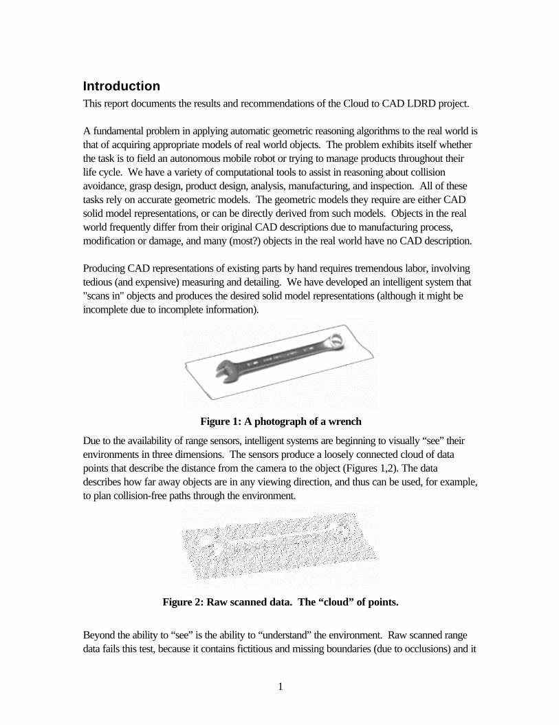
Producing CAD representations of existing parts by hand requires tremendous labor, involvingtedious (and expensive) measuring and detailing. We have developed an intelligent system that"scans in" objects and produces the desired solid model representations (although it might beincomplete due to incomplete information).

Figure 1: A photograph of a wrench

Due to the availability of range sensors, intelligent systems are beginning to visually “see” theirenvironments in three dimensions. The sensors produce a loosely connected cloud of datapoints that describe the distance from the camera to the object (Figures 1,2). The datadescribes how far away objects are in any viewing direction, and thus can be used, for example,to plan collision-free paths through the environment.

Figure 2: Raw scanned data. The “cloud” of points.

Beyond the ability to “see” is the ability to “understand” the environment. Raw scanned rangedata fails this test, because it contains fictitious and missing boundaries (due to occlusions) and it

2

fails to explicitly represent surface curvature. A robot can use range information to avoidcollisions, but will have difficulty manipulating objects because the data neither says that a bolt isround nor that it is separate from the table it is laying on. A wide variety of current geometricreasoning capabilities, including assembly and fixture planning, currently rely on CAD solidmodel data. Raw scanned data currently cannot support such applications.

Figure 3: A CAD model of the wrench.

The information we seek is implicit in the scanned range data; people are able to determine theshapes of objects in a scene merely by looking.

Previous WorkAt the inception of this project, most of the previous work had been performed at universities.Current university work [1] focused on producing a solid model by using scan facets directly forsolid model faces, without computing exact surfaces. Multiple views were accounted for byperforming Boolean intersections of solids produced from each view. Such an approachproduces incredibly complex models, which require hours to process and still lack the exactsurfaces required for use beyond visualization and production of crude approximations of realparts. Other work in the area focused mainly on producing surface models from scanned data,stopping far short of closed boundary representation topology.

3

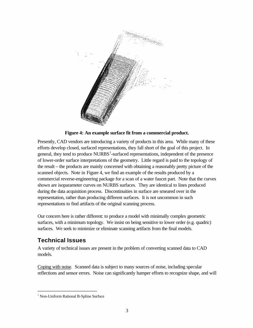
Figure 4: An example surface fit from a commercial product.

Presently, CAD vendors are introducing a variety of products in this area. While many of theseefforts develop closed, surfaced representations, they fall short of the goal of this project. Ingeneral, they tend to produce NURBS1-surfaced representations, independent of the presenceof lower-order surface interpretations of the geometry. Little regard is paid to the topology ofthe result – the products are mainly concerned with obtaining a reasonably pretty picture of thescanned objects. Note in Figure 4, we find an example of the results produced by acommercial reverse-engineering package for a scan of a water faucet part. Note that the curvesshown are isoparameter curves on NURBS surfaces. They are identical to lines producedduring the data acquisition process. Discontinuities in surface are smeared over in therepresentation, rather than producing different surfaces. It is not uncommon in suchrepresentations to find artifacts of the original scanning process.

Our concern here is rather different: to produce a model with minimally complex geometricsurfaces, with a minimum topology. We insist on being sensitive to lower order (e.g. quadric)surfaces. We seek to minimize or eliminate scanning artifacts from the final models.

Technical IssuesA variety of technical issues are present in the problem of converting scanned data to CADmodels.

Coping with noise. Scanned data is subject to many sources of noise, including specularreflections and sensor errors. Noise can significantly hamper efforts to recognize shape, and will

1 Non-Uniform Rational B-Spline Surface

4

affect the accuracy of the final results. Thus, means for minimizing the impact of noise will berequired.

Integrating data from multiple viewpoints. From a single viewpoint, it is only possible to viewthe visible side of an object. Any surfaces of the object that don’t face the sensor will bemissing from the model. Multiple sensor views can be used to fill in gaps in the model, but theymust be reconciled with each other.

Segmenting the model. Scanned data provides a map of coordinates on the surface of themodel, but does not distinguish between different surfaces of a part or between surfaces ofdifferent parts. It is necessary to partition the scanned points into groups that can be associatedwith CAD model surfaces, and these groups are not known a priori.

Dealing with multiple geometric interpretations. Scanned data is subject to a vast number ofgeometric interpretations. At one extreme, every three adjacent points can define a planarfacet, which will produce models with large numbers of planar faces (Figure 4). At anotherextreme, the grid of sample points could define the basis for one large, extremely complex splinesurface. Neither extreme case is “correct”, because correctness (for design and analysispurposes) requires the model to have a minimum number of surfaces of minimum complexity.Algorithms for proposing geometric interpretations must be very efficient in exploring variousinterpretations.

Achieving model closure. CAD systems require closed models. Even with multiple views, it ispossible for a model to lack some surfaces (e.g. surfaces in contact). Creating completelybounded manifold solid models requires the ability to construct artificial boundaries. A moresubtle solid model closure issue relates to edges. Edges define the intersection of surfaces, soadjacent surfaces must have equations of a form that produces well-defined edges. A globaladjustment of surface equations might be necessary to insure valid edge definition.

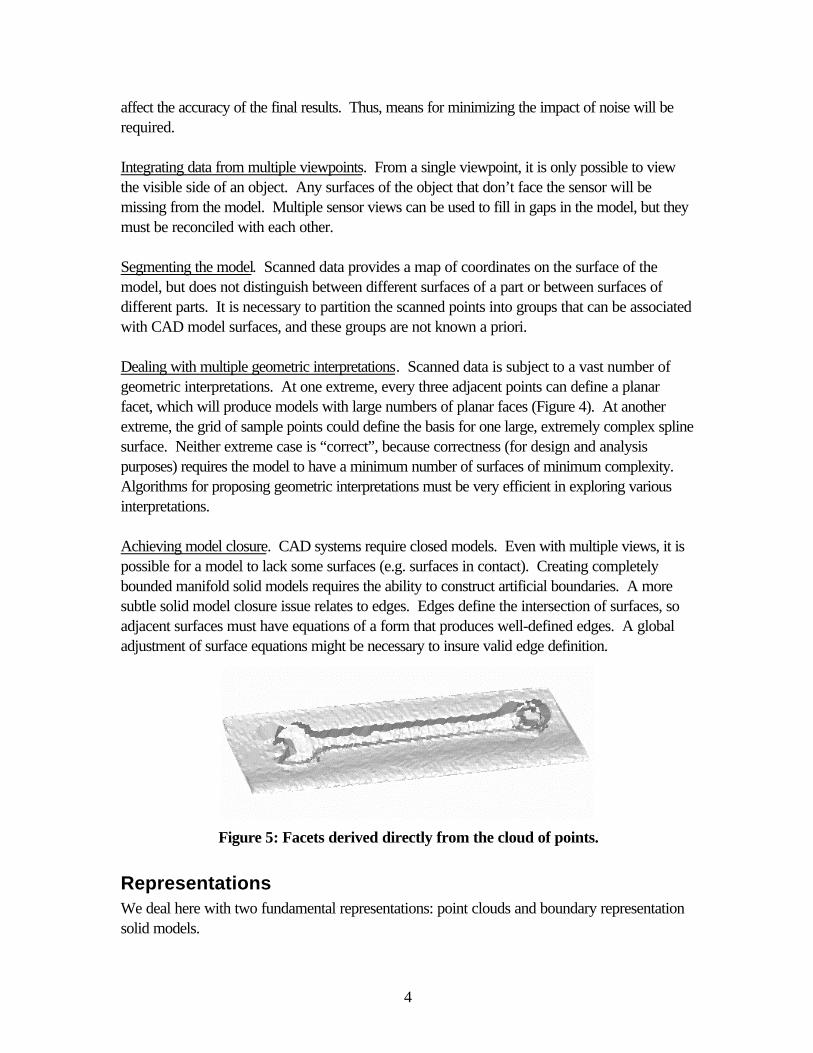
Figure 5: Facets derived directly from the cloud of points.

RepresentationsWe deal here with two fundamental representations: point clouds and boundary representationsolid models.

5

Point CloudThe data produced by a scanned range system is typically referred to as a “point cloud”. Apoint cloud is a collection of points, together with a loosely defined topology. The points aretypically three-dimensional data, defined in a coordinate system relative to the scanner (orrelative to a larger world coordinate system that the scanner is positioned within). The looselydefined topology is an artifact of the scanning process. A scanner acquires point data bysweeping through the scene. At any given instant, some collection of points is produced.Adjacency between points is determined either by geometric proximity or by some adjacencydefined by the scanner (e.g. adjacent pixels in a camera suggest some adjacency. It is possible,due to occlusion, reflection, noise, and a variety of other effects, for points to be “missing” – noreturn to the sensor occurs where we might expect adjacent points to be. Where points areclose, both topologically and geometrically, it is possible to infer adjacency.

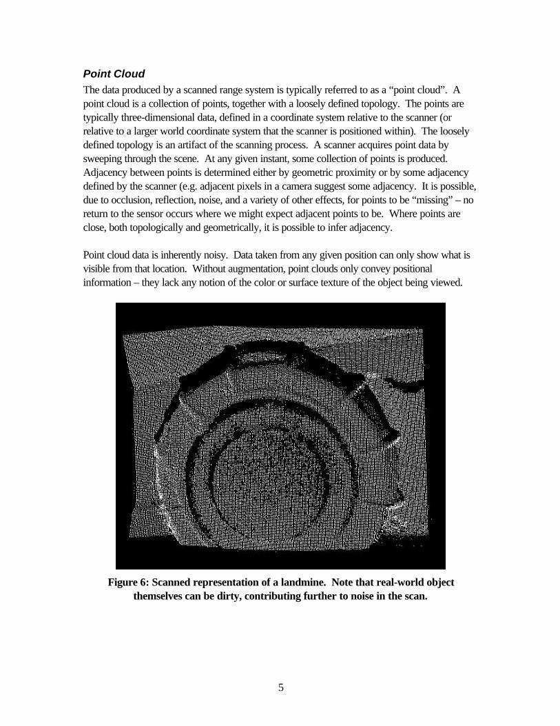
Point cloud data is inherently noisy. Data taken from any given position can only show what isvisible from that location. Without augmentation, point clouds only convey positionalinformation – they lack any notion of the color or surface texture of the object being viewed.

Figure 6: Scanned representation of a landmine. Note that real-world objectthemselves can be dirty, contributing further to noise in the scan.

6

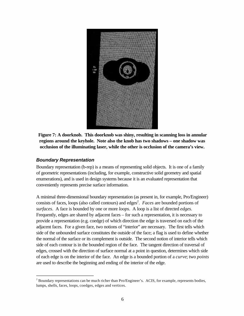
Figure 7: A doorknob. This doorknob was shiny, resulting in scanning loss in annularregions around the keyhole. Note also the knob has two shadows – one shadow wasocclusion of the illuminating laser, while the other is occlusion of the camera’s view.

Boundary RepresentationBoundary representation (b-rep) is a means of representing solid objects. It is one of a familyof geometric representations (including, for example, constructive solid geometry and spatialenumerations), and is used in design systems because it is an evaluated representation thatconveniently represents precise surface information.

A minimal three-dimensional boundary representation (as present in, for example, Pro/Engineer)consists of faces, loops (also called contours) and edges2. Faces are bounded portions ofsurfaces. A face is bounded by one or more loops. A loop is a list of directed edges.Frequently, edges are shared by adjacent faces – for such a representation, it is necessary toprovide a representation (e.g. coedge) of which direction the edge is traversed on each of theadjacent faces. For a given face, two notions of “interior” are necessary. The first tells whichside of the unbounded surface constitutes the outside of the face; a flag is used to define whetherthe normal of the surface or its complement is outside. The second notion of interior tells whichside of each contour is in the bounded region of the face. The tangent direction of traversal ofedges, crossed with the direction of surface normal at a point in question, determines which sideof each edge is on the interior of the face. An edge is a bounded portion of a curve; two pointsare used to describe the beginning and ending of the interior of the edge.

2 Boundary representations can be much richer than Pro/Engineer’s. ACIS, for example, represents bodies,lumps, shells, faces, loops, coedges, edges and vertices.

7

Each surface is represented by a geometric equation, typically in parametric (rather than implicit)form. CAD systems typically represent the following types of surface: plane, cylinder, sphere,cone, torus, and NURBS (non-uniform rational b-spline surface). In engineered objects, thenatural quadric surfaces (plane, cylinder, cone, sphere) occur much more frequently than free-form surfaces.

Each curve is also represented as a geometric equation, typically in parametric form. CADsystems ordinarily represent the following types of curves: line, ellipse, and spline. Note that foreach type of surface-surface intersection, it is possible to use a specific type of curve (e.g.parabolas and hyperbolas for cone-plane intersection). In practice, CAD systems use splinecurves for most types of intersection (other than lines and ellipses), and frequently onlyapproximate the true intersection curve.

CAD systems ordinarily represent exact, idealized geometry – that is, geometry as the designerwould wish given a perfect world. For example, the angle of intersection between two planeswould typically be 90°, and not 89° or 91°.

ApproachThe problem of extracting solid model data from scanned models can be viewed as arecognition problem: given a low-level representation of information, attempt to recognizehigher-level patterns. The recognition process involves partitioning the point set into collectionsthat define surfaces, finding intersections of those surfaces to produce edge equations, stitchingsurfaces at edges, and adjusting surfaces and adding new surfaces to improve closure.

Importing scanned data points directly into a CAD system (as either points or polygons) was abasic first milestone. Such representations may seem unimportant, but this data is appropriate incases where the scan represents non-designed geometry (e.g. a hip joint in a medicalapplication), where parts are designed to interface to scanned geometry without beingcomposed of it.

Next, we developed algorithms that search the point/facet information to determine a collectionof surfaces (e.g. planes, cylinders) that bound the object. Hints such as adjacency andsimilarity of surface normals will be used to limit the amount of search required. We willaccount for noise in the scanned points by allowing tolerance in the surface fitting algorithms. Atthis point, models consisting of disconnected surfaces can be produced.

After surface representations could be proposed, we proceeded with the task of bounding thesurfaces and determining adjacency. Producing solid model topology requires defining edgegeometry that correctly represents intersections between adjacent surfaces. In some cases,surface intersections are not well formed due to noise in the data, so surface parameters (or thesurface recognition algorithms) can require modification to form a reasonable model.

8

In support of robotic recognition applications, we began work to search a database of modelsbased on the scanned surface data. Some progress was made there.

Directly Importing Triangles into a CAD SystemPrevious work (e.g. [Little96]) with scanned range data has produced relatively stabletriangulating algorithms. Given that basis, we simply constructed faceted solid models from thetriangulations, and imported them into CAD algorithms.

As expected, the triangulations render reasonably well, albeit slowly. Most CAD constructionoperations are unwieldy with such representations, as a great deal of selecting must occur toperform a simple operation like selecting a face. Many operations, such as mass-propertiescalculation, take far longer than the same operations on models using many fewer faces havinghigher-order surface equations. Thus, we are driven by the desire for efficient representation toseek the higher-order representations.

Figure 5 shows the results of importing triangles directly into a CAD system. The results aredifficult to use, but could be acceptable if nothing else is available.

Not shown (due to difficulty visualizing the data) is a scanned representation of an automobiletire. We computed mass properties directly from scanned data for the tire. Mass propertiescomputation for a solid model of a complete tire required roughly 20 minutes; mass propertiesfor the faceted scanned representation required 1-1/2 days. Even the model construction of thefaceted representation was slow, requiring 8 hours (4 if we eliminated sharing of adjacent edges,essentially producing a surface model rather than a solid).

Surface FittingThe current surface representations of choice in CAD systems include planes, natural quadricsurfaces, tori and NURBS. Some systems use NURBS exclusively, but more frequently thesystems use the lower-order special cases as they occur frequently in design. Estimates rangethat as high as 80 percent of all the designed surfaces in mechanical parts are planar or quadric,so they certainly form an important class of surfaces to recognize. Quadric surfaces provideremarkable representational efficiency, as they possess closed-form solutions for many of thegeometric queries required.

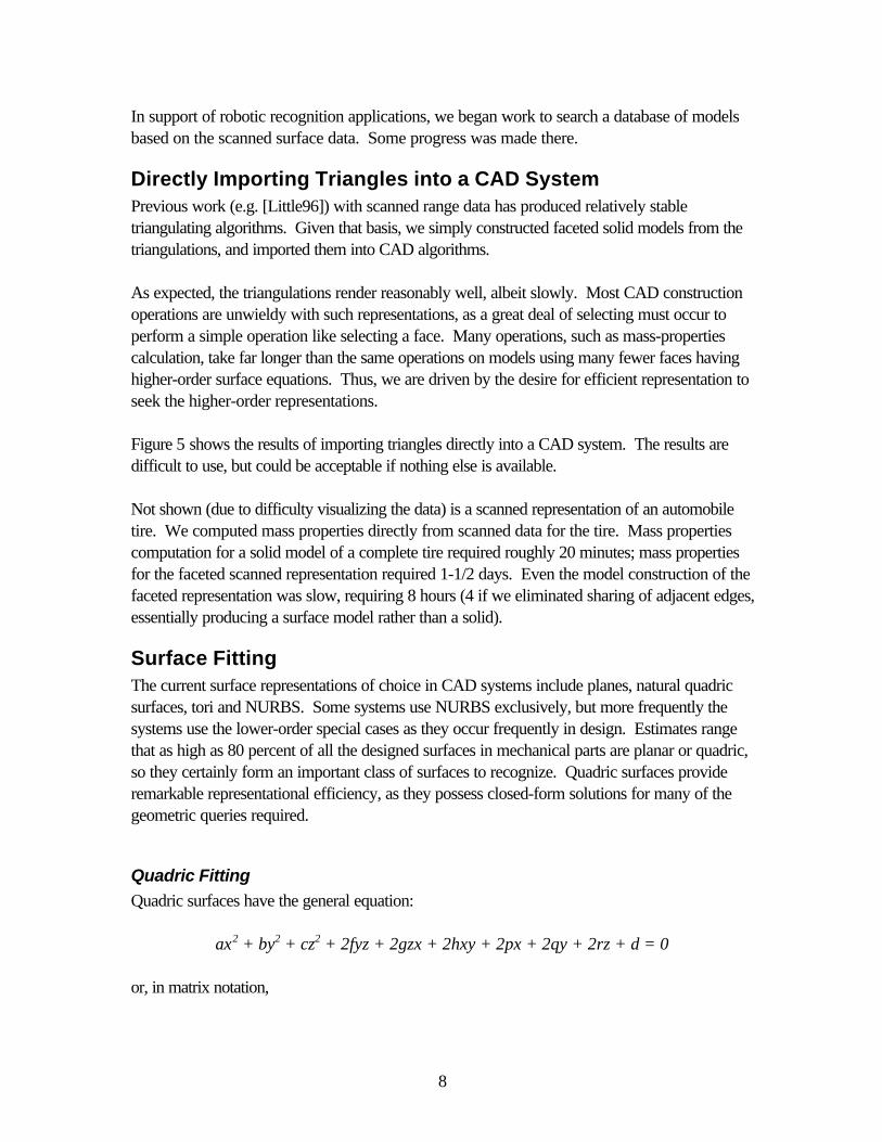
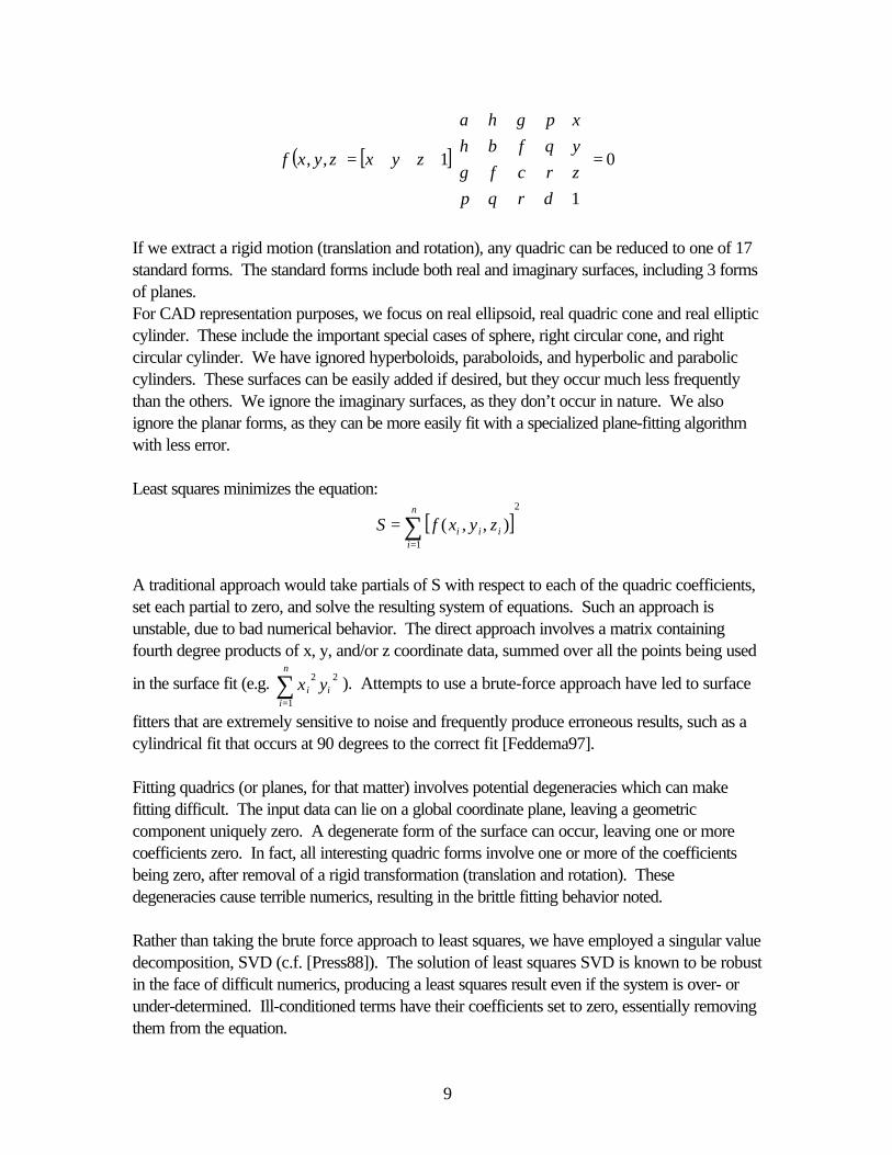
Quadric FittingQuadric surfaces have the general equation:

ax2 + by2 + cz2 + 2fyz + 2gzx + 2hxy + 2px + 2qy + 2rz + d = 0

or, in matrix notation,

9

( ) [ ] 0

1

1,, =

=zyx

drqprcfgqfbhpgha

zyxzyxf

If we extract a rigid motion (translation and rotation), any quadric can be reduced to one of 17standard forms. The standard forms include both real and imaginary surfaces, including 3 formsof planes.For CAD representation purposes, we focus on real ellipsoid, real quadric cone and real ellipticcylinder. These include the important special cases of sphere, right circular cone, and rightcircular cylinder. We have ignored hyperboloids, paraboloids, and hyperbolic and paraboliccylinders. These surfaces can be easily added if desired, but they occur much less frequentlythan the others. We ignore the imaginary surfaces, as they don’t occur in nature. We alsoignore the planar forms, as they can be more easily fit with a specialized plane-fitting algorithmwith less error.

Least squares minimizes the equation:

[ ]2

1

),,(∑=

=n

iiii zyxfS

A traditional approach would take partials of S with respect to each of the quadric coefficients,set each partial to zero, and solve the resulting system of equations. Such an approach isunstable, due to bad numerical behavior. The direct approach involves a matrix containingfourth degree products of x, y, and/or z coordinate data, summed over all the points being used

in the surface fit (e.g. ∑=

n

iii yx

1

22 ). Attempts to use a brute-force approach have led to surface

fitters that are extremely sensitive to noise and frequently produce erroneous results, such as acylindrical fit that occurs at 90 degrees to the correct fit [Feddema97].

Fitting quadrics (or planes, for that matter) involves potential degeneracies which can makefitting difficult. The input data can lie on a global coordinate plane, leaving a geometriccomponent uniquely zero. A degenerate form of the surface can occur, leaving one or morecoefficients zero. In fact, all interesting quadric forms involve one or more of the coefficientsbeing zero, after removal of a rigid transformation (translation and rotation). Thesedegeneracies cause terrible numerics, resulting in the brittle fitting behavior noted.

Rather than taking the brute force approach to least squares, we have employed a singular valuedecomposition, SVD (c.f. [Press88]). The solution of least squares SVD is known to be robustin the face of difficult numerics, producing a least squares result even if the system is over- orunder-determined. Ill-conditioned terms have their coefficients set to zero, essentially removingthem from the equation.

10

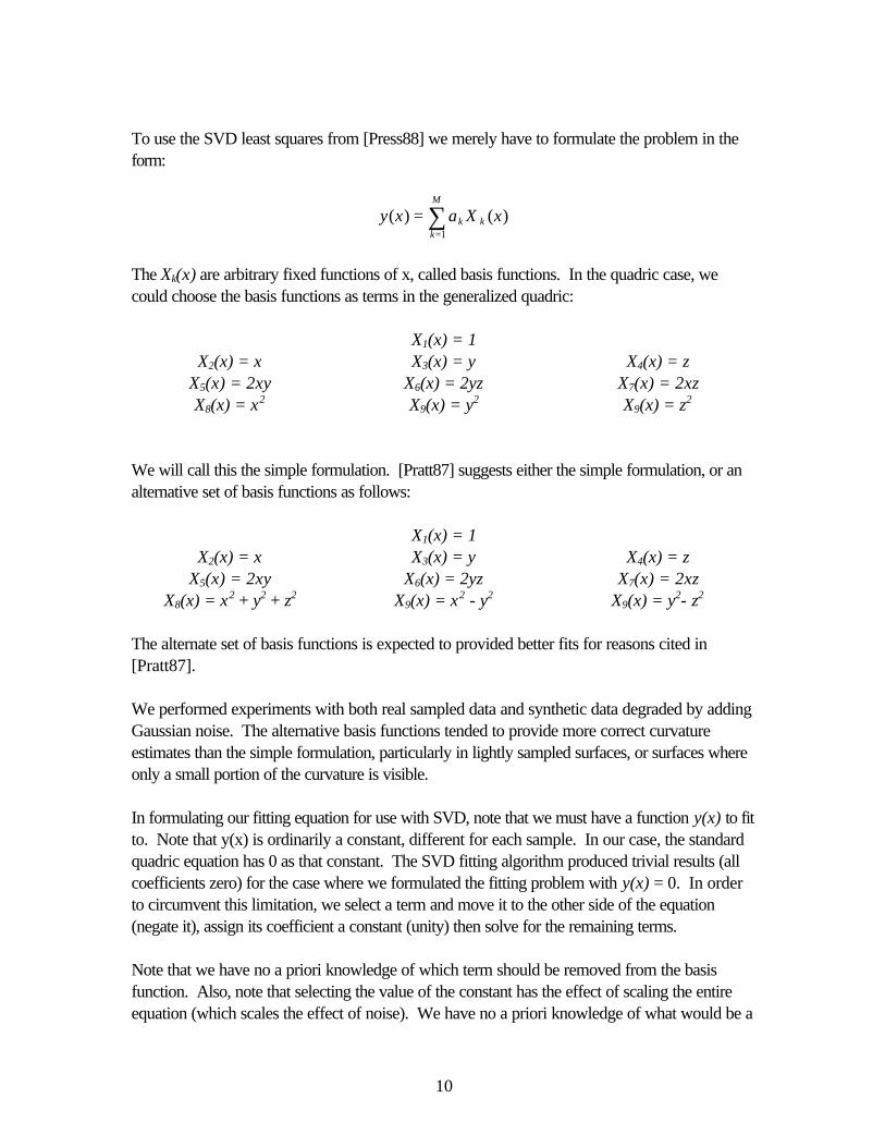
To use the SVD least squares from [Press88] we merely have to formulate the problem in theform:

∑=

=M

kkk xXaxy

1

)()(

The Xk(x) are arbitrary fixed functions of x, called basis functions. In the quadric case, wecould choose the basis functions as terms in the generalized quadric:

X1(x) = 1X2(x) = x X3(x) = y X4(x) = z

X5(x) = 2xy X6(x) = 2yz X7(x) = 2xzX8(x) = x2 X9(x) = y2 X9(x) = z2

We will call this the simple formulation. [Pratt87] suggests either the simple formulation, or analternative set of basis functions as follows:

X1(x) = 1X2(x) = x X3(x) = y X4(x) = z

X5(x) = 2xy X6(x) = 2yz X7(x) = 2xzX8(x) = x2 + y2 + z2 X9(x) = x2 - y2 X9(x) = y2- z2

The alternate set of basis functions is expected to provided better fits for reasons cited in[Pratt87].

We performed experiments with both real sampled data and synthetic data degraded by addingGaussian noise. The alternative basis functions tended to provide more correct curvatureestimates than the simple formulation, particularly in lightly sampled surfaces, or surfaces whereonly a small portion of the curvature is visible.

In formulating our fitting equation for use with SVD, note that we must have a function y(x) to fitto. Note that y(x) is ordinarily a constant, different for each sample. In our case, the standardquadric equation has 0 as that constant. The SVD fitting algorithm produced trivial results (allcoefficients zero) for the case where we formulated the fitting problem with y(x) = 0. In orderto circumvent this limitation, we select a term and move it to the other side of the equation(negate it), assign its coefficient a constant (unity) then solve for the remaining terms.

Note that we have no a priori knowledge of which term should be removed from the basisfunction. Also, note that selecting the value of the constant has the effect of scaling the entireequation (which scales the effect of noise). We have no a priori knowledge of what would be a

11

good choice for that scaling. We also lack knowledge of which terms will be zero, andremoving zero-valued terms from the basis has no useful effect on the solution of the fittingproblem (we have a problem because of the zero in the equation).

We opted for an approach that solves reduced basis functions. We iterate through the terms inthe original basis function. For each term, we construct a reduced basis function which is simplythe original function with the term removed. The coefficient of the term in question is set to 1,and the system solved. We then examine the resulting surface fits and determine which solutionfits the data best. We determine goodness-of-fit by summing the distance of each point in thesample from the surface we have found. The surface with least error is the solution of choice.3

Experiments in adding noise to the surfaces showed that as the noise increased, the number ofcorrect solutions found decreased, but that degradation of the algorithm was gradual. Sufficientexperiments were not performed to precisely quantify the degree of noise permitted.

Plane FittingWe used a lower-order form of the same equations for fitting planes. Recall that the generalequation is ax + by + cz + d = 0. In this case, we chose to use X1(x) = 1, X2(x) = x + y + z,X3(x) = x - y, X4(x) = y – z as the basis functions. This choice was forced by circumstance.We encountered scanned data where the scanner was aimed directly at a flat reference surfacex = 0. This is a very degenerate case: all of the x coordinate data is zero, the y and z arearbitrary, but with zero coefficients b and c, and the constant d is only correct if zero. If we usethe simple formulation, we cannot find an appropriate term to remove from the basis, becauseevery term ends up zero in one way or another. The alternate formulation forces more terms tobe non-zero, permitting the fitting to occur.

The specialized plane fitting algorithm was developed because the quadric fitting algorithm didnot simplify well to planar fits. The effect of noise permitted nonlinear terms to be found by thefitting algorithm much sooner for the quadric formulation than was experienced with thespecialized planar fitting algorithm. In practice, both algorithms are used, but only non-planarquadrics are sought for comparison to the specialized planar solutions.

Determination of Surface Type[Zwillinger96] provides a recipe for identifying the type of quadric given a quadric in generalform. The approach involves constructing a matrix form of the quadric and its first derivative,computing matrix ranks, eigenvalues and determinants, and performing a table lookup based onmatrix ranks, sign of a determinant, and the number of sign changes in the eigenvalues. In

3 Note that the SVD produces a measure of error, χ2, which could be used to compare solutions. Attempts tocompare solutions based on that error measure were not sufficiently reliable; this problem might be due tothe immature state of our algorithms at the time those attempts were made.

12

practice, noise in the parameters can cause near-zero conditions for some of the matrixparameters, making the determination of surface type sensitive to noise.

Our solution involved determining surface parameters for each surface type of interest,independent of classification. The errors associated with each surface type were measured andthe best fitting surface was chosen. In cases where the parameters were clearly unreasonable(e.g. negative radius), no surface was constructed for comparison.

Determination of Surface ParametersInformation on determining the values of surface parameters was provided by [Levy00]. Thecenter of central quadrics is found by taking the partial derivatives of the quadric equation,setting to zero, and solving for the center (x0, y0, z0) of the quadric. This solution is equivalent todetermining the solution of the matrix equation

0=

zyx

cfgfbhgha

The principal axes and parameters related to those axes can be determined directly from aneigenvalue analysis of the matrix of coefficients above. Each eigenvector is a dominant vector ofthe quadric; its associated eigenvalue is the square of the reciprocal of the associated parameter(i.e. radius) in that direction. A case-by-case analysis of each interesting quadric is required toextract the relevant parameters.

Surface-Fitting Based SegmentationOur approach to segmentation is very similar to [Besl88]. Our work directly uses the surfacefitting algorithms to drive segmentation. The approach is simple – take a small collection ofpoints, fit a surface, and attempt to extend the surface by adding points that belong to the initialgroup. It is necessary to begin with a sufficiently large group to permit the surface fittingalgorithm to operate (Nyquist criteria), while at the same time carefully avoiding the possibility ofcrossing edges of the object. We try a number of starting places within a geometric region. Wetake the best grouping and grow surfaces from it, if we find a sufficiently accurate fit.

Problems with initially choosing too small a patch for fitting can result in a surface that is self-limiting. Consider a cylinder for which we choose a collection of points that are sufficiently smallthat a plane is fit. In growing the surface, points that would encourage the cylindrical fit to befavored are rejected as they don’t belong to the plane that was originally fit. For this reason, wefavor initial patches that are significantly larger than the surface-finding algorithm requires. Thisrequirement drives us towards fine sampling of points. It also can produce problems in regionshaving many very small surfaces. In such cases, we have to acknowledge that tiny surfaces arebeyond recognition.

13

Each group of points is associated to a solid model face, by attribute attachment. The errorassociated with each point can be conveniently stored along with the point. This informationpermits querying of the resultant model to determine whether and where there are opportunitiesfor more detailed scanning, should a higher degree of accuracy be required.

Grouping close points for beginning the segmentation process requires an efficient model fordetermining proximity. An efficient model for this is traversing a triangulation of the point set tolocate close points. The scanning hardware itself can suggest appropriate models fortriangulation. If multiple scans must be triangulated, something like Delaunay triangulation isappropriate. The triangulation reduces the search for adjacent entities to an O(1) algorithm,which is necessary for propagation to be fast.

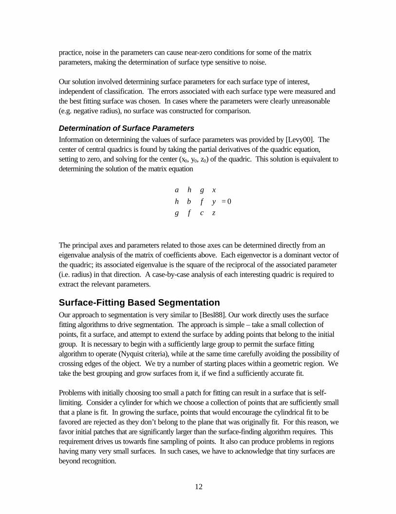
Figure 8: CAD model used for generating synthetic data.

14

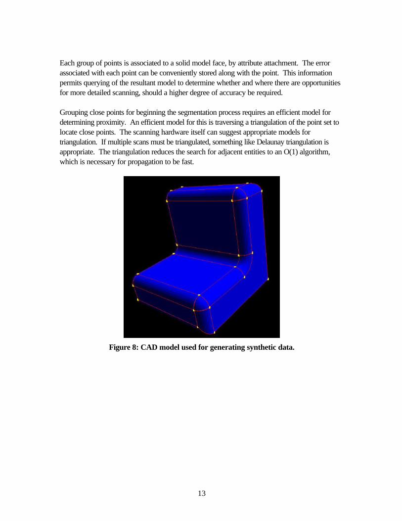
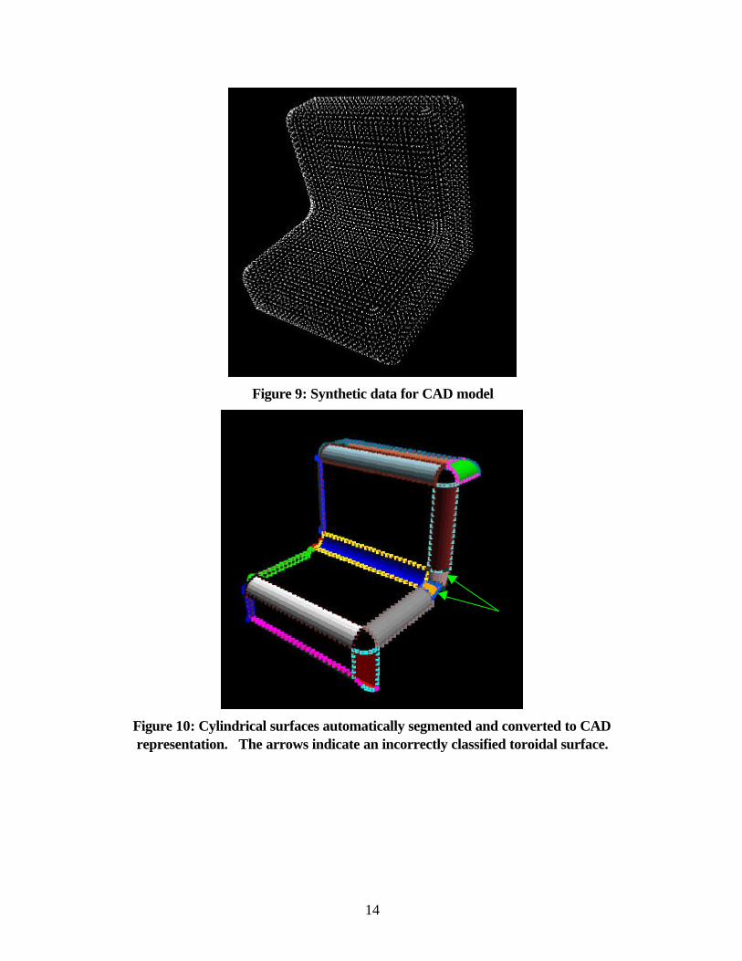
Figure 9: Synthetic data for CAD model

Figure 10: Cylindrical surfaces automatically segmented and converted to CADrepresentation. The arrows indicate an incorrectly classified toroidal surface.

15

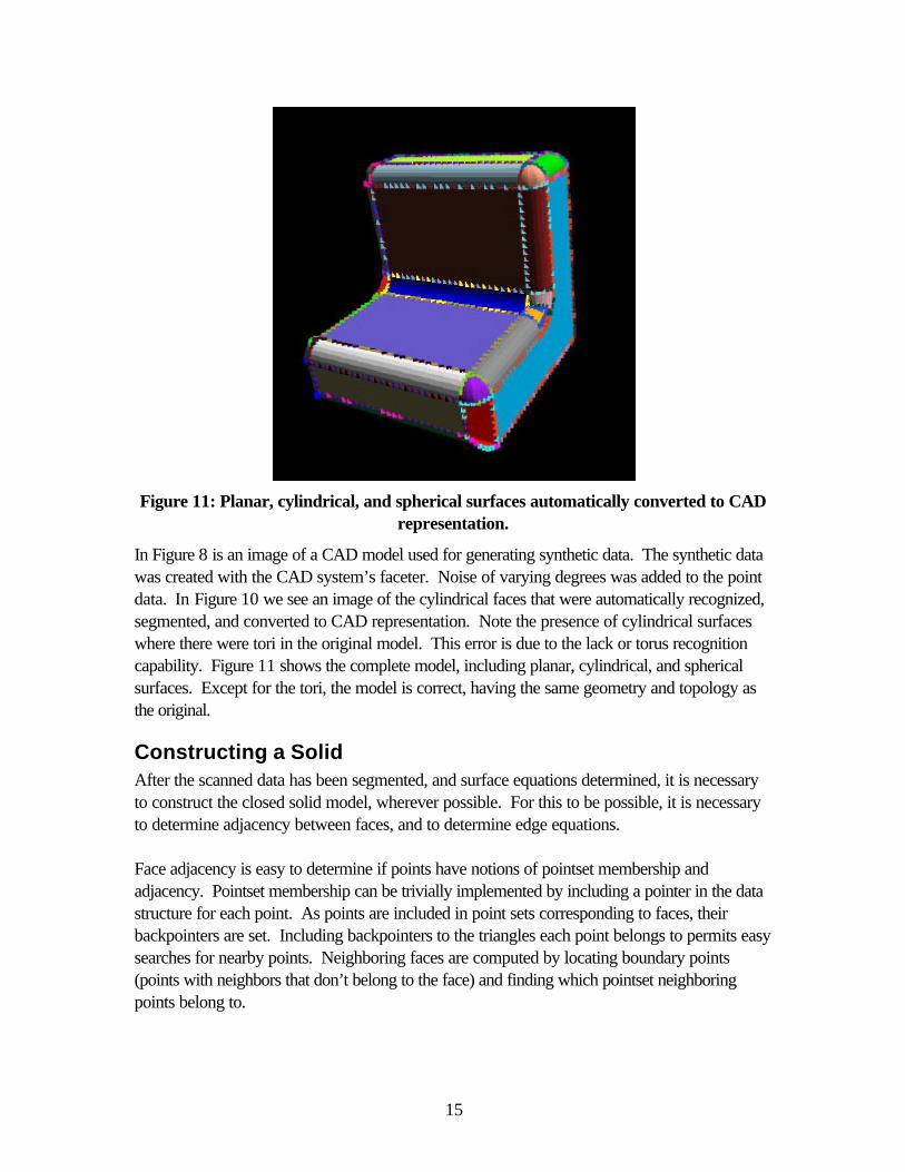
Figure 11: Planar, cylindrical, and spherical surfaces automatically converted to CADrepresentation.

In Figure 8 is an image of a CAD model used for generating synthetic data. The synthetic datawas created with the CAD system’s faceter. Noise of varying degrees was added to the pointdata. In Figure 10 we see an image of the cylindrical faces that were automatically recognized,segmented, and converted to CAD representation. Note the presence of cylindrical surfaceswhere there were tori in the original model. This error is due to the lack or torus recognitioncapability. Figure 11 shows the complete model, including planar, cylindrical, and sphericalsurfaces. Except for the tori, the model is correct, having the same geometry and topology asthe original.

Constructing a SolidAfter the scanned data has been segmented, and surface equations determined, it is necessaryto construct the closed solid model, wherever possible. For this to be possible, it is necessaryto determine adjacency between faces, and to determine edge equations.

Face adjacency is easy to determine if points have notions of pointset membership andadjacency. Pointset membership can be trivially implemented by including a pointer in the datastructure for each point. As points are included in point sets corresponding to faces, theirbackpointers are set. Including backpointers to the triangles each point belongs to permits easysearches for nearby points. Neighboring faces are computed by locating boundary points(points with neighbors that don’t belong to the face) and finding which pointset neighboringpoints belong to.

16

Approximating edges can be constructed from the edges of the triangulation. Such aconstruction will, of course, contain scanned artifacts, but this is of necessity in regions wherethe scan is incompletely closed. Boundaries constructed directly from scanned data arespecifically marked as being approximate both for use by downstream applications and for usein fitting together scans from multiple viewpoints. These fictitious boundaries are principalcandidates for regions in which data from multiple views will be merged.

“Exact” edge equations can, in principal, be determined by intersecting the surface equations ofneighboring faces. Tangent surfaces pose a special problem, as it is possible for tangentsurfaces to lack any intersection. Tangent edges can be computed on a case-wise basis (e.g.plane/cylinder, cylinder/sphere), but for sufficiently large gaps the resultant solids will not survivemany of the geometric operations they might have to endure (e.g. Boolean intersections). Webegan work in this area, completing the direct intersections, but were unable to work on tangentintersections. Loops constructed from these computed edges were unfortunately unavailable atthe end of the project for technical reasons.

Bounding loops of faces are simply computed by locating bounding edges and constructingminimal loops via a minimal spanning tree algorithm. Note that these loops can be constructedout of a combination of exact edges and scanned-data edges, depending on whether thescanned data forms a complete model.

Note that the solids created here might be incomplete, due to occlusion. It may not be possibleto scan from a sufficient number of views to find closure faces if the object being scannedcannot be adequately manipulated. It is also possible to have a problem segmenting betweenseparate objects. Neither of these subjects were adequately investigated due to fundingshortfall.

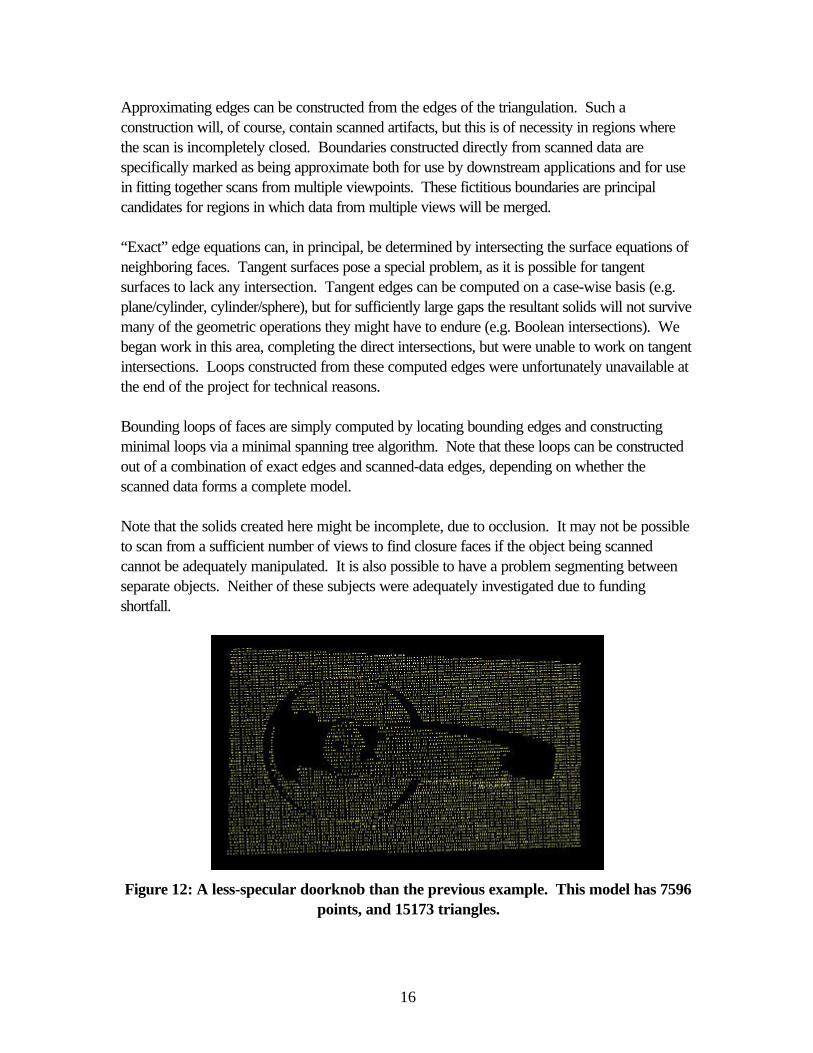
Figure 12: A less-specular doorknob than the previous example. This model has 7596points, and 15173 triangles.

17

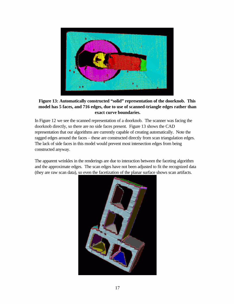
Figure 13: Automatically constructed “solid” representation of the doorknob. Thismodel has 5 faces, and 716 edges, due to use of scanned-triangle edges rather than

exact curve boundaries.

In Figure 12 we see the scanned representation of a doorknob. The scanner was facing thedoorknob directly, so there are no side faces present. Figure 13 shows the CADrepresentation that our algorithms are currently capable of creating automatically. Note theragged edges around the faces – these are constructed directly from scan triangulation edges.The lack of side faces in this model would prevent most intersection edges from beingconstructed anyway.

The apparent wrinkles in the renderings are due to interaction between the faceting algorithmand the approximate edges. The scan edges have not been adjusted to fit the recognized data(they are raw scan data), so even the facetization of the planar surface shows scan artifacts.

18

Figure 14: Two cinderblocks. Note that the cinderblocks are not segmented from eachother, due to lack of sufficient information in the range data. Additional information is

necessary to complete the segmentation.

Searching Previously Defined ModelsClearly, for constructing a complete solid it is necessary to have data from a sufficient number ofviews to permit construction of the complete manifold. Where such complete data isunavailable, we have the choice of working with an incompletely closed model, searching forpreviously defined models, or extrapolating the model to achieve closure.

We began work on algorithms for searching to locate previously modeled CAD data. Thesearch involves extracting defining parameters (e.g. plane normal, cylinder axis) from surfaces,edges, and/or vertices, and comparing the scanned model to a collection of previouslydeveloped CAD models.

The most reliable information from the scan is surface information. The surface equations areconstructed from fitting large numbers of points, negating a significant amount of noise. Noise isstill present, and both surface classification and surface parameters can be affected. Edgeinformation less reliable, as it is constructed from intersections of surfaces – if the surfaces areinaccurate, the edges are likely to be more inaccurate. Moreover, edge information may simplybe absent -- for incomplete visibility, it is possible that no surface/surface intersections areavailable for computing edges. Vertices are even more problematic, as we require the presenceof three or more faces to properly define a vertex. The point-cloud-based model is thusincomplete and somewhat inaccurate.

Solid models contain many vertices that are arbitrarily placed, such as the vertex linking the startof a periodic curve to its end. The placement of such a vertex is either dictated by theparametric representation of the curve, or might be entirely arbitrary. Comparison algorithmsmust be careful such artifacts in vertex, edge, and surface data. Edge and face data in CAD isotherwise quite reliable. CAD models frequently show surface, curve, and vertexcorrespondence of 10e-6, far better than we expect from scanned data. CAD data can exhibitstrange construction artifacts, such as small slivers. It is necessary to confine our comparisonsto the largest faces to avoid searching for modeling artifacts.

We are left with the comparison of sketchy, incomplete data to precise, likely completely closedmodels. Also, the largest, most important faces in the CAD model might be those that wereoccluded in the scanned data.

We began an algorithm for making these comparisons. We extract surface descriptors: planenormal and origin (corrected for uniqueness by passing a line through the origin); cylinder radiusand axis; sphere center and radius; and cone origin, axis, and half angle. These descriptors areassociated with the surface area of each face in the model, as well as with a representation of

19

adjacency. The descriptors are constructed for both models. We sort the faces in the point-cloud-derived model, and begin from the largest. We search the CAD model for similar faces,and seek as soon as possible to orient the model. Continue matching faces until we have areasonable match, or until failure occurs.

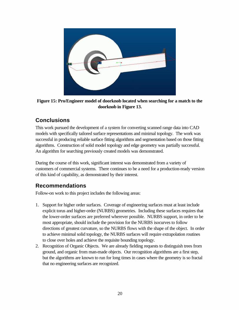
The searching algorithm worked reasonably well for a small sampling of surfaces, but has notbeen exercised with a large number of CAD models. We created a small database of CADmodels of objects, including the object in Figure 15, and searched for the doorknob in Figure13. The doorknob was correctly found, even though we lacked any side face information.Planar faces in such views are a significant problem, as they are difficult to orient without thepresence of orthogonal faces (which might be absent in a single view) or reasonable edges(which can only be approximated without the presence of adjacent faces).

20

Figure 15: Pro/Engineer model of doorknob located when searching for a match to thedoorknob in Figure 13.

ConclusionsThis work pursued the development of a system for converting scanned range data into CADmodels with specifically tailored surface representations and minimal topology. The work wassuccessful in producing reliable surface fitting algorithms and segmentation based on those fittingalgorithms. Construction of solid model topology and edge geometry was partially successful.An algorithm for searching previously created models was demonstrated.

During the course of this work, significant interest was demonstrated from a variety ofcustomers of commercial systems. There continues to be a need for a production-ready versionof this kind of capability, as demonstrated by their interest.

RecommendationsFollow-on work to this project includes the following areas:

1. Support for higher order surfaces. Coverage of engineering surfaces must at least includeexplicit torus and higher-order (NURBS) geometries. Including these surfaces requires thatthe lower-order surfaces are preferred wherever possible. NURBS support, in order to bemost appropriate, should include the provision for the NURBS isocurves to followdirections of greatest curvature, so the NURBS flows with the shape of the object. In orderto achieve minimal solid topology, the NURBS surfaces will require extrapolation routinesto close over holes and achieve the requisite bounding topology.

2. Recognition of Organic Objects. We are already fielding requests to distinguish trees fromground, and organic from man-made objects. Our recognition algorithms are a first step,but the algorithms are known to run for long times in cases where the geometry is so fractalthat no engineering surfaces are recognized.

21

3. Reduce Sensitivity to Noise. Insufficient time was available for a complete characterizationof the algorithms relative to noise. The current algorithms are robust in the face of noise,and appear to degrade gracefully, but more work to guarantee this is warranted.

4. Testing with Many Large Models. Our test suite was significant, but more, larger modelsare necessary to validate the system.

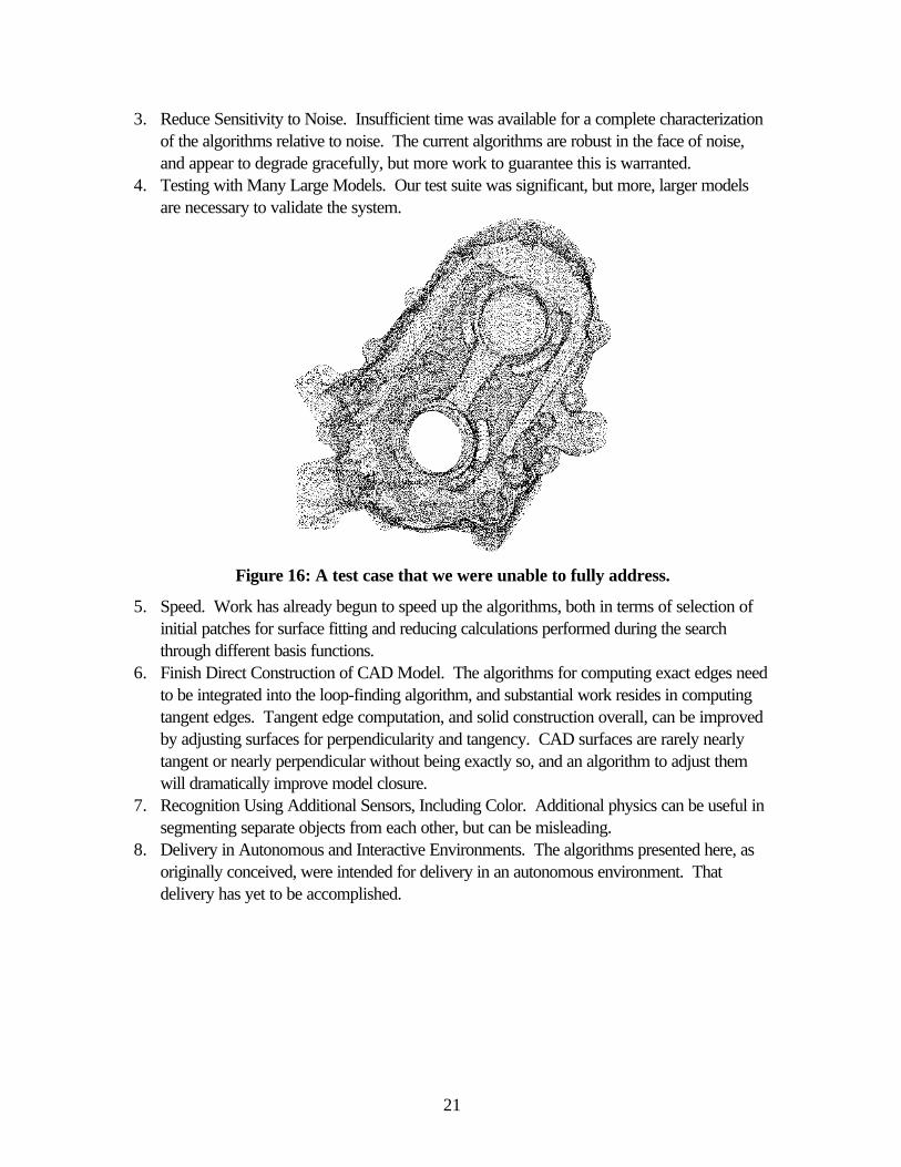
Figure 16: A test case that we were unable to fully address.

5. Speed. Work has already begun to speed up the algorithms, both in terms of selection ofinitial patches for surface fitting and reducing calculations performed during the searchthrough different basis functions.

6. Finish Direct Construction of CAD Model. The algorithms for computing exact edges needto be integrated into the loop-finding algorithm, and substantial work resides in computingtangent edges. Tangent edge computation, and solid construction overall, can be improvedby adjusting surfaces for perpendicularity and tangency. CAD surfaces are rarely nearlytangent or nearly perpendicular without being exactly so, and an algorithm to adjust themwill dramatically improve model closure.

7. Recognition Using Additional Sensors, Including Color. Additional physics can be useful insegmenting separate objects from each other, but can be misleading.

8. Delivery in Autonomous and Interactive Environments. The algorithms presented here, asoriginally conceived, were intended for delivery in an autonomous environment. Thatdelivery has yet to be accomplished.

22

References[Allen97] Allen, P. K., and Reed, M. K., “A Robotic System for 3D Model Acquisition

from Multiple Range Images”, Proceedings of IEEE InternationalConference on Robotics and Automation, Albuquerque, NM, April 1997.

[Besl88] Besl, P. J., Jain, R.C., “Segmentation Through Variable-Order Surface Fitting"”IEEE Transactions on Pattern Analysis and Machine Intelligence, Vol. 10,No. 2, March 1988.

[Feddema97] Feddema, J. and Little, C., “Rapid World Modeling: Fitting Range Data toGeometric Primitives”, Proceedings 1997 IEEE International Conference onRobotics and Automation, Albuquerque, NM, 1997.

[Levy00] Levy, S., Personal Communication, March 2000.

[Little96] Little, C., Wilson, C. W., “Rapid World Modelling for Robotics”, WorldAutomation Congress ‘96 Proceedings, May 1996.

[Pratt87] Pratt, V., “Direct Least-Squares Fitting of Algebraic Surfaces”, ComputerGraphics, Volume 21, Number 4, Association for Computing Machinery, July1987.

[Press88] Press, W. H., Teukolsky, S. A., Vetterling, W. T., Flannery, B. P., NumericalRecipes in C: The Art of Scientific Computing, Second Edition, CambridgeUniversity Press, New York, NY, 1988.

[PTC95] Pro/Develop Reference Guide, Release 16, Parametric TechnologyCorporation, Waltham, MA, 1995.

[Requicha80] Requicha, A.A.G., “Representations for rigid solids: Theory, methods, andsystems”, ACM Computing Surveys, 12(4): 437-464, December 1980.

[Spatial98] ACIS 4.0 Online Help CD, Spatial Technology Corporation, Boulder,Colorado, 1998.

[Zwillinger96] Zwillinger, D., ed., CRC Standard Mathematical Tables and Formulae, 30th

Edition, CRC Press, Boca Raton, Fl., 1996.

23

Distribution

Internal Distribution:

MS1002 P. J. Eicker, 15200

MS1010 M. E. Olson, 15222

MS1010 A. L. Ames, 15222, 20 copies

MS1010 D. M. Hensinger, 15222

MS1010 D. K. Kholwadwala, 15222

MS1008 P. G. Xavier, 15221

MS1003 C. Q. Little, 15211

MS1003 C. Lewis, 15211

MS1004 R. R. Peters, 15221

MS0188 LDRD Office, 1030

MS9018 Central Technical Files, 8945-1

MS0899 Technical Library, 9616, 2 copies

MS0612 Review & Approval Desk, 9612 For DOE/OSTI