Closed Chamber Well Test Analysis by Superposition of the … · test as often does a conventional...

Stanford Geothermal Program Interdisciplinary Research in

Engineering and Earth Sciences STANFORD UNIVERSITY

Stanford, California

S GP-TR-8 7

CLOSED CHAMBER WELL TEST ANALYSIS BY SUPERPOSITION OF THE CONSTANT PRESSURE CUMULATIVE INFLUX SOLUTION TO THE RADIAL DlFFUSlVlTY EQUATION

BY

Jeffrey F. Simmons

February 1985

Financial support was provided through t h e Stanford Geothermal Program under Department of Energy Contract

No. DE-AT03-80SF11459 and by the Department of Petroleum Engineering, Stanford University

- ii -

1: ABSTRACT

A computer Program was developed to model the closed chamber test. Super-

position Of the Constant pressure cumulative influx solution was utilized to avoid

the problems associated with direct solution of the governing partial differential

equations.

The model was tested for the ability to generate a slug test response and

then used to illustrate the difference between the slug test and closed chamber

test.

A sensitivity study was conducted by varying tool and reservoir parameters

from a control basecase. Unlike the slug test, initial fluid level, initial chamber gas

pressure, and produced fluid gravity greatly influence the closed chamber pres-

sure response. As a result, the slug test dimensionless group t D / CD is ineffective

in collapsing the closed chamber curves. Assuming ideal chamber gas behavior did

to not slgnificantly influence the closed chamber pressure response.

The developed superposition model was used t o generate dimensionless type

curves for a particular tool and reservoir situation. A log-log plot of pD versus to,

analogous to the late time slug test format of Ramey et. al (19761, yields the

greatest sensitivity to skin analysis.

. iii .

CONTENTS

Paae

1 . ABSTRACT ................................................................................................................. t i

2 . INTRODUCTION ........................................................................................................ 1

2.1 General Description ..................................................................................... 1

2.2 Previous Work .............................................................................................. 5

3 . PROPOSED SOLUTION METHOD .............................................................................. 8

3.1 Overview and Assumptions ........................................................................ 8

3.2 Constant Pressure Cumulative Influx ....................................................... 10

3.3 Superposition t o Determine Influx ............................................................ 13

3.4 Calculation of the Closed Chamber Test Response ............................... 16

3.5 Type Curve Analysis ................................................................................... 21

4 . VERIFICATION OF CLOSED CHAMBER MODEL ........................................................ 33

4.1 Slug Test Duplication .................................................................................. 33

4.2 Closed Chamber Variance from Slug Test ................................................ 35

6 . NUMERICAL CONSIDERATIONS ................................................................................ 43

6.1 Time Step Selection .................................................................................... 43

5.2 Improvements in Efficiency of Time Step ................................................ 47

8 . SENSITIVITY STUDY ................................................................................................. 49

6.1 Effect of Produced Fluid Gravity .............................................................. 60

6.2 Effect of Chamber Gas Gravity ................................................................. 52

6.3 Effect of Initial Liquid Level ...................................................................... 52

6.4 Effect of Initial Chamber Pressure ........................................................... 53

6.5 Effect of Total Chamber Length ............................................................... 54

8.6 Effect of Chamber Diameter 5~

6.7 Effect of Reservoir Sand Thickness ........................................................ 65

6.8 Effect of Initial Reservoir Pressure .......................................................... 56

E ......................................................................

... ’

. Iv .

6.9 Effect of Chamber Gas Temperature ....................................................... 56

6.10 Effect of Assuming Ideal Gas Behavior .................................................. 57

7 . CONCLUSIONS AND RECOMMENDATIONS .............................................................. 89

8 . NOMENCLATURE ........................................................................................................ 93

REFERENCES ..................................................................................................................... 96

APPENDIX A COMPUTER PROGRAM ............................................................................... 97

APPENDIX B BASECASE NUMERICAL VALUES ............................................................... 108

2: INTRODUCTION

2.1 General Description

Closed chamber well testing is common in the petroleum industry today in the

guise of backsurge perforation cleaning. In oil producing regions of the world

where sand control is required, backsurging is often performed prior to gravel

packing of the productive interval as a means of cleaning debris from the perfora-

tions. First introduced in the U.S. Gulf Coast, backsurging has proven successful

in providing more productive completions.

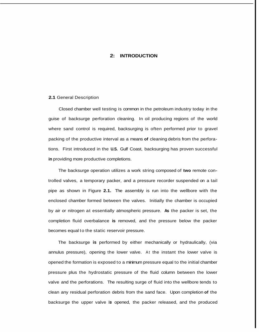
The backsurge operation utilizes a work string composed of two remote con-

trolled valves, a temporary packer, and a pressure recorder suspended on a tail

pipe as shown in Figure 2.1. The assembly is run into the wellbore with the

enclosed chamber formed between the valves. Initially the chamber is occupied

by air or nitrogen at essentially atmospheric pressure. As the packer is set, the

completion fluid overbalance is removed, and the pressure below the packer

becomes equal to the static reservoir pressure.

The backsurge is performed by either mechanically or hydraulically, (via

annulus pressure), opening the lower valve. A t the instant the lower valve is

opened the formation is exposed to a minimum pressure equal to the initial chamber

pressure plus the hydrostatic pressure of the fluid column between the lower

valve and the perforations. The resulting surge of fluid into the wellbore tends to

clean any residual perforation debris from the sand face. Upon completion of the

backsurge the upper valve Is opened, the packer released, and the produced

Drill Works

Gas liquid -

Perforations \

- 2 -

f Lower Surge Ualue

/ Pressure Recorder

Figure 2.1 Mechanical Sketch o f Backsurge Equipment

fluids are reverse circulated out of the wellbore.

The pressure response form the backsurge is commonly recorded with an

Amerada Hess type recorder to verify that a successful draw down was achieved.

A typical pressure response from a successful backsurge is presented in Figure

2.2.

E f i! k S 0

T I K

Figure 2.28 Typicol Pressure Response

As the tool assembly is run into the well, the pressure bomb records the increase

in hydrostatic pressure. Setting the packer relieves the completion fluid overbal-

ance, and the bottom hole pressure becomes equal to the static reservoir pres-

sure. When the lower surge valve is opened the draw down is obtained, and fluids

are produced. As the fluid level rises, the bottom hole pressure approaches the

static reservoir pressure. The packer Is then released, returning the bottom hole

pressure to an overbalance. Reverse circulation of produced fluids causes a

momentary pressure increase prior to pulling the tool assembly out of the well.

- 4 -

A reduced ineffective draw down results when either a valve, the packer or

drill pipe fail t o seal. If an acceptable draw down was achieved during the opera-

tion, the pressure data is often utilized only as a measure of the initial reservoir

pressure.

Permeability and Skin Analysis

The intent of this report is to present a method of analyzing backsurge pres-

sure data to determine oil reservoir parameters of permeability and Hurst skin

effect. Knowledge of these parameters will yield greater efficiency of field

development. Closed chamber well testing provides a safer method of obtaining

permeabiltity and skin values in areas often considered unsuitable for conventional

drill stem analysis, No surface pressure build up occurs during a closed chamber

test as often does a conventional drill stem test. Conventional drill stem tests are

seldom utilized in geopressured offshore oil fields for fear of well control problems.

The closed chamber well test is a more generalized form of the drill stem test

known as the slug test. Analogous to the slug test, a closed chamber well test

begins with the instantaneous removal of a volume of liquid from the wellbore. The

resulting decrease in bottom hole pressure causes an immediate influx of reservoir

fluids. As the removed fluid volume is replaced the bottom hole pressure increases

due to the hydrostatic pressure of the rising liquid column. For the closed chamber

test, the additional upper valve results in a compressing gas volume on top of the

rising fluid level. The effect is to produce continuous changing well bore storage

through out the test. Because of the gas compression, the bottom hole pressure

increases much faster than in the case of the slug test. In both cases the ever

increasing back pressure on the formation continually decreases the flow rate at

the sand face until the bottom hole pressure reaches the static reservoir pres-

sure.

- 6 -

Permeability and skin analysis of the slug test by type curve match has pro-

ven a valid solution technique. Yet attempts to analyze closed chamber well test

data by type curve matching with published slug test dimensionless solutions are

often impossible. Because the slug test assumption of constant wellbore storage

is greatly violated, as the gas compression becomes significant, late time closed

chamber pressure data deviates from the equivalent slug test response.

The deviation is often so severe that two thirds of a closed chamber test

response must be neglected in order to match the early time response with the

slug test of the correct transmissibility. In the rare case of a closed chamber

test of a low pressured formation using a long chamber containing low initial

chamber pressure, a large portion of the pressure response would be analogous to

the slug test and suitable for analysis by slug test type curve match. But, in gen-

eral, such an approach in inappropriate and may yield erroneous results.

2.2 PREVIOUS WORK

Slug Test

A detailed derivation of the slug test solution, including skin effect, was

presented in 1972 by Ramey and Agarwal. The method of solution by Laplace

transformation was similar to the solution of the heat transfer problem of a

cylinder with a heat resistance (skin effect). Solution to the heat transfer problem

was presented by Jaeger in 1956. The slug test solution was obtained by

neglecting momentum, friction, phase change, and wellbore fluid compressibility

changes.

In 1975, Ramey, Agarwal, and Martin reduced the slug test solution to a set

of dimensionless curves using the concept of effective wellbore radius. Although

somewhat empirical, the correlation effectively collapsed the slug test data using

the parameter C’eZS. Slug test analysis is obteined by type curve matching with

1

- 6 -

the collapsed set of curves.

Closed Chamber Test

Alexander, in 1977 suggested analysis of closed chamber well test data as a

qualitative method of designing conventional drill stem tests. Alexander proposed

conducting a closed chamber well test initially to determine the produced fluid pro-

perties and expected flow rates of new wells. The closed chamber test results

would then be used in the design of the conventional drill stem test equipment and

to determine the necessary flow period of the test.

In 1980 Shinohara presented a detailed analytic solution to the closed

chamber test problem. The inner boundary condition for the radial diffusivity equa-

tion was derived by applying a momentum balance to the rising fluid level within

the well bore. A dimensionless solution was obtained by assuming the gas column

length insignificant compared to the initial fluid column height. With this assump-

tion, and assuming ideal chamber gas behavior, variations of the slug test dimen-

sionless variables may be derived, resulting in a nondimensional diffusivity equa-

tion. The resulting partial differential equations were found t o be nonlinear an

unsuitable for solution by Laplace transformation. Solution was obtained numeri-

cally using a finite difference scheme. Although momentum effects were con-

sidered in the formulation, wellbore friction, phase change, and compressibility of

the wellbore fluids were considered negligible.

Saldana, in 1983, presented a detailed study of a generalized drill stem test

formulation including friction and momentum effects. A general equation was pro-

posed to analyze various test scenarios. For each test situation the general equa-

tion coefficients were defined to adapt the generalized equation. A closed

chamber well test was considered by substituting specific coefficients. As with

Shinohara's approach, ideal gas behavior was assumed to facilitate the use of

dimensionless variables. It is not clear what other assumptions were required to

- 7 -

obtain the numerical solutions offered for several examples.

3: PROPOSED SOLUTION METHOD

9.1 Overview and Assumptions

Even with the assumption of ideal gas behavior, previous solutions of the

closed chamber well test problem by Shinohara and Saldana, have resulted in

non-linear partial differential equations. The non-linearity results from the con-

tinuous changing well bore storage present through out the test caused by the

compressing column of gas above the rising fluid level interface. Numerical tech-

niques have been required to evaluate the pressure response governed by the

non-linear partial differential equations.

The method of closed chamber well test analysis presented In this report utii-

ltes superposition to avoid the limitations required when solving the diffusivity

equation in the presence of changing well bore storage. Analysis by superposition

makes possible the inclusion of non-ideal chamber gas behavior and places no

restrictions on the well bore geometry. Because the approach is not analytic, a

dimensionless general solution is not presented. But because fewer restriction are

required for solution, the influence of independent test parameters can be studied

as a guide to future analysis.

Many assumptions are still required in the superposition formulation which fol-

lows. To avoid ambiguity, the limitations of the proposed model are presented first

in the development. It is assumed that:

1) No phase change occurs between the produced liquids and the chamber gas.

Furthermore it is assumed that all solution gas remains dissolved in the liquid

phase during the test period.

I

- 9 -

2) Wellbore liquids are considered incompressible. The chamber gas compressi-

bility is assumed much greater than the produced liquid compressibility.

3) Momentum effects are not considered in the model.

4) Friction effects are not considered in the model.

6) Critical flow does not impede the flow rate during the test period.

6) Only liquid is produced from the reservoir during the test.

7 ) Throughout the test period, the reservoir behaves as an infinite homogeneous

radial system of constant thickness.

8 ) Total formation compressibility is constant and independent of pressure.

8 ) Gradient of pressure with respect to depth can be neglected in the gas

column.

10) Gradient of temperature with respect to depth can be neglected in the gas

column.

- 1 0 -

3.2: Constant Pressure Cumulative Influx

Governing Equations

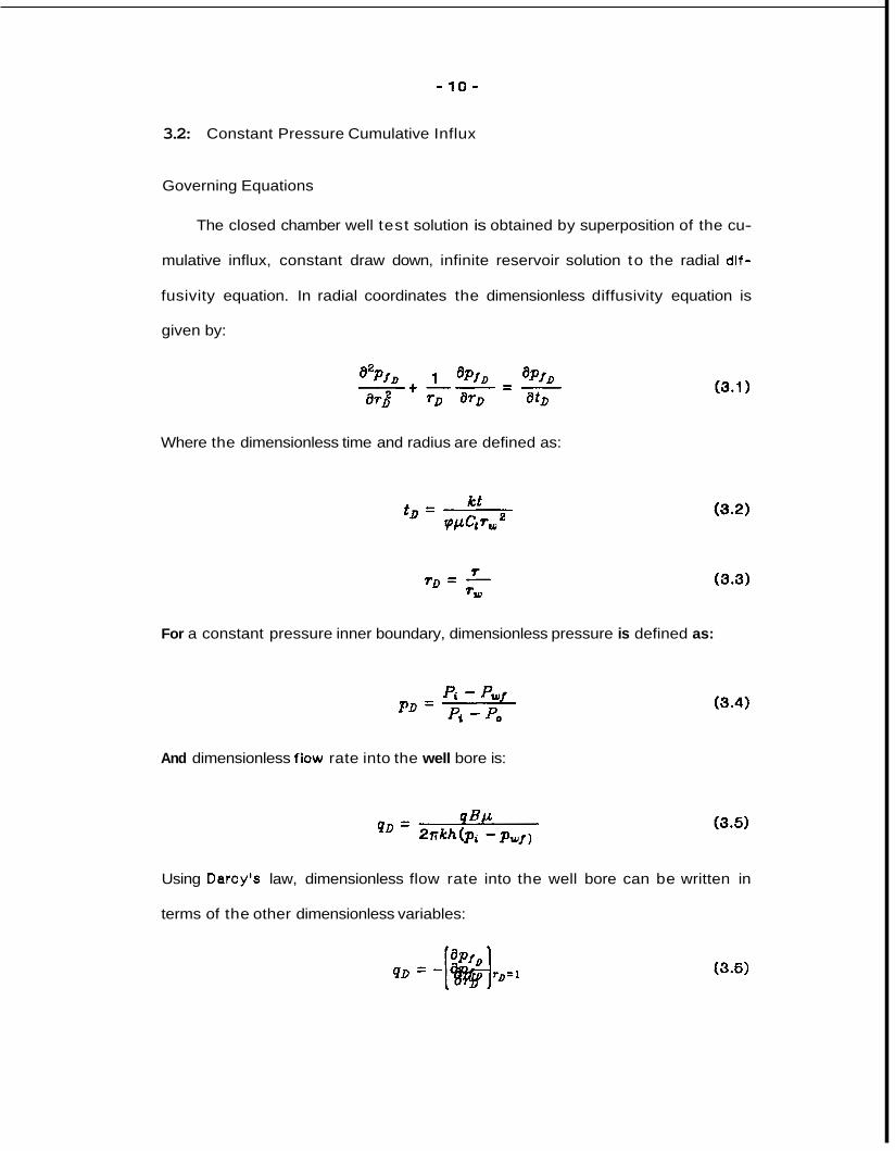
The closed chamber well test solution is obtained by superposition of the cu-

mulative influx, constant draw down, infinite reservoir solution to the radial dif-

fusivity equation. In radial coordinates the dimensionless diffusivity equation is

given by:

Where the dimensionless time and radius are defined as:

For a constant pressure inner boundary, dimensionless pressure is defined as:

And dimensionless flow rate into the well bore is:

Using Darcy's law, dimensionless flow rate into the well bore can be written in

terms of the other dimensionless variables:

40 = -1-1 apf 8TD D rD=1

- 11 -

Dimensionless cumulative influx is defined as:

Initial and Boundary Conditions

The reservoir is considered at static equilibrium prior to the onset of constant

pressure draw down. A t t =0, p =pi at all T . In terms of dimensionless variables:

A t the outer boundary, the reservoir is considered to behave as if infinite during

the test:

lim P D ( ~ D , ~ D ) = 0 (3.9) rD -Sw

Additional pressure drop at the sand face due to damage or stimulation is con-

sidered with the van Everdingen and Hurst dimensionless skin factor:

In dimensionless terms corresponding to the definitions given above:

The Inner boundary is

dimensionless terms:

(3.1 0 )

(3.1 1)

constant pressure. For all time greater than t =O; pwf =pa . In

(3.1 2)

-12-

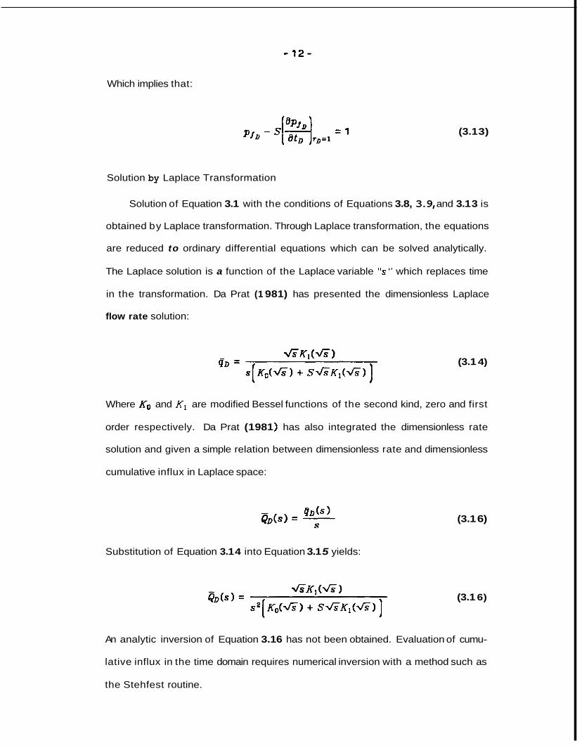
Which implies that:

(3.1 3)

Solution by Laplace Transformation

Solution of Equation 3.1 with the conditions of Equations 3.8, 3.9, and 3.1 3 is

obtained by Laplace transformation. Through Laplace transformation, the equations

are reduced to ordinary differential equations which can be solved analytically.

The Laplace solution is a function of the Laplace variable "s" which replaces time

in the transformation. Da Prat (1 981) has presented the dimensionless Laplace

flow rate solution:

(3.1 4)

Where KO and K1 are modified Bessel functions of the second kind, zero and first

order respectively. Da Prat (1 981 ) has also integrated the dimensionless rate

solution and given a simple relation between dimensionless rate and dimensionless

cumulative influx in Laplace space:

Substitution of Equation 3.1 4 into Equation 3.1 5 yields:

(3.1 6)

(3.1 6)

An analytic inversion of Equation 3.16 has not been obtained. Evaluation of cumu-

lative influx in the time domain requires numerical inversion with a method such as

the Stehfest routine.

- 1 3 -

3.3 Superposition t o Determine Cumulative Influx

Dimensionless cumulative influx for a constant pressure draw down can be

evaluated by numerical inversion of Equation 3.1 6. To relate dimensionless cumu-

lative Influx to influx a constant of proportionality is defined:

B = 2nphCtTz

Then, for the case of constant pressure draw down:

Q ( t ) = Bba -PufIBo( tD)

Where t~ is calculated using the time the draw down is in effect.

(3.1 7 )

(3.1 8 )

Pressure Draw Down Variation

During a closed chamber well test, the flowing pressure at the sand face

varies as the fluid level rises with in the well bore. Superposition of the constant

pressure, cumulative influx solution allows the cumulative influx from a radial sys-

tem to be calculated given a well bore pressure history.

Figure 3.1: Variable Pressure Response

- 1 4 -

To perform the calculation the continuous pressure response is discretized into

constant pressure intervals of short duration. Because the radial diffusivity equa-

tion is linear for a constant pressure inner boundary, the individual response to

each constant pressure interval may be summed together to determine the net in-

flux at a given time.

Consider the pressure response presented in Figure 3.1. The time scale is

discretized into equal time increments. To determine the influx after time increment

"N", the draw down pressure response is represented as a series of step func-

tions:

Figure 3.88 Constant Draw Down Representation

Because a forward looking calculation is required to model the closed chamber test

response, the initial draw down at the beginning of each time step is assumed to

remain constant over the time step interval. Accurate representation of the actual

response requires that the time increment be small, such that the pressure change

per time step is insignificant compared to the pressure.

- 15 -

Cumulative influx after time step “N” is calculated by superposing the effect

of each time step. After time step “N“, the pressure drop Ip, - p , ] has been in ef-

fect for the total time. Successive pressure changes must be subtracted during

the corresponding time in effect. Fluid produced after ”N” time steps may be

represented as:

Where A t 0 is evaluated based on the time step A t .

- 16 -

9.4 Calculation of the Closed Chamber Test Response

Using the concept of superposition as presented in the preceding section,

cumulative fluid influx at given time can be calculated from a known pressure draw

down history. With the assumption that the pressure change per time step is

small, the superposition technique can be extented to calculate the fluid influx at

one time step past the last pressure history value. Then knowing the cumulative

influx, the bottom hole flowing pressure can be calculated from the well bore

geometry and fluid properties. The pressure history is updated and the two step

process repeated to generate the pressure response,

The chamber gas pressure can be calculated from the initial gas pressure as-

suming the type of compression. If the compression occurs rapidly with out time for

significant heat transfer, the process could be treated as adiabatic. Annular fluids

and the surrounding rock would tend to maintain an isothermal process if compres-

sion occurs slow enough to allow for heat dissipation. The actual process Is prob-

ably somewhere between adiabatic and isothermal, with limited heat transfer dur-

ing the test period. Subsequent sensitivity studies, presented in this report, have

shown gas temperature variance does not significantly alter the bottom hole pres-

sure calculation. For simplicity, isothermal gas compression is assumed.

Consider the well bore geometry of Figure 3.3. Assuming the chamber cross

sectional area constant, with respect to depth, the chamber gas pressure can be

calculated from the ideal gas law. For isothermal compression of a constant molar

quantity of gas:

The chamber volume, l/Eh, may be expressed as:

(3.20)

(3.21)

- 1 7 -

Dynamic Liquid Leuel

x 1 C

lnitia Leuel

I Liquid

Figure 3.3 Geometry Defining Uariebles

- 1 8 -

Substituting Equation 3.21 into 3.20 and rearranging, yields an expression for

chamber pressure as a function of fluid level X:

(3.22)

The real gas 2 factor was calculated, assuming hydrocarbon gas composition, us-

ing the Brill and Breggs correlation. Because Z is a function of the calculation

of p c h was iterative. Convergence was reached when the change in 2 per itera-

tion was less than 0.01 X .

The fluid level, X, can be calculated form the cumulative fluid influx:

X = & + - N &h

(3.23)

Assuming momentum and friction effects are insignificant within the well bore, the

bottom hole pressure is equal to the chamber gas pressure plus the hydrostatic

pressure of liquid column:

(3.24)

For a given value of fluid influx, Equations 3.22, 3.23, and, 3.24 allow calcu-

lation of the flowing well bore pressure. Thus the pressure at one time step past

the known pressure history can be calculated from the fluid influx as calculated

by Equation 3.1 9.

In retrospect, the pressure response is generated as follows:

1) Assume the flowing pressure during time step "N" is equal to the pressure at

the start of the time step, ' @ N - I ' ' .

2) Calculate the cumulative fluid influx at the end of time step "N" using Equa-

tion 3.19.

- 19 -

3) Calculate the fluid level at the end of time step "N" using Equation 3.23.

4) Calculate the chamber pressure at the end of step "N" using Equation 3.22.

Iteration is necessary because Z is a function of pch.

6) Calculate the bottom hole pressure at the end of time step "N" using Equa-

tion 3.24.

0 ) Update the pressure history, index, and return to step number 1).

Figure 3.4 presents the computer flow chart of the superposition closed chamber

model.

- 20 -

Calculate the Cumulative

Fluid Influx at the

Calculate

Fluid Level

,I + J

Calculate Chamber Pressure Using Most Recent

Value of 2

CdlCUldtQ New VdlUQ O f

Using the New

, Chamber Pressure

I

Calculate the Bottom Hole Pressure from

Hydrostatics

Assume the Bottom Hole Pressure is 1 b

Constant for Current NO Time Step

I

I Update

Cumulative

Record

2 0 .ooo 1

Figure 3.4 Computer Progrem Flow Chart

- 2 1 -

5.5 Type Curve Analysis

The algorithm proposed in the preceding section provides a method of gen-

erating the pressure response of a closed chamber test, for a given set of tool

and reservoir parameters. Evaluation of unknown reservoir parameters requires ap-

plication of a history matching technique. As previously discussed, type curve

analysis has proven to be a practical method of slug test evaluation. Closed

chamber test response data were therefore plotted on coordinate axes used by

Ramey et. al. (1 976) for slug test analysis.

Slug Test

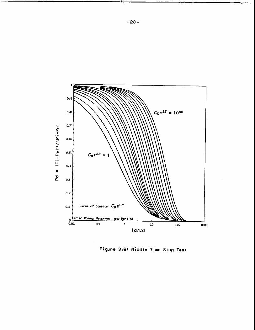
In 1975, Ramey, Agawal, and Martin proposed type curve plotting of slug

test data on three coordinate systems. Dimensionless pressure was found to be a

function of only two parameters: C’eZs and t ~ / CD . Thus a single set of curves

provides the general slug test solution. Each coordinate system emphasizes sensi-

tivity to a particular time range of the data.

Analysis of field data is obtained by plotting dimensionless pressure versus

time and type curve matching with the dimensionless solutions. Transmissibility is

calculated from the time match. Skin effect is obtained by curve shape match

with a dimensionless curve of constant C’ezs. To interpret the entire slug test

response, three plots are requlred. Slug test type curves are presented in Figure

3.5,3.6, and 3.7.

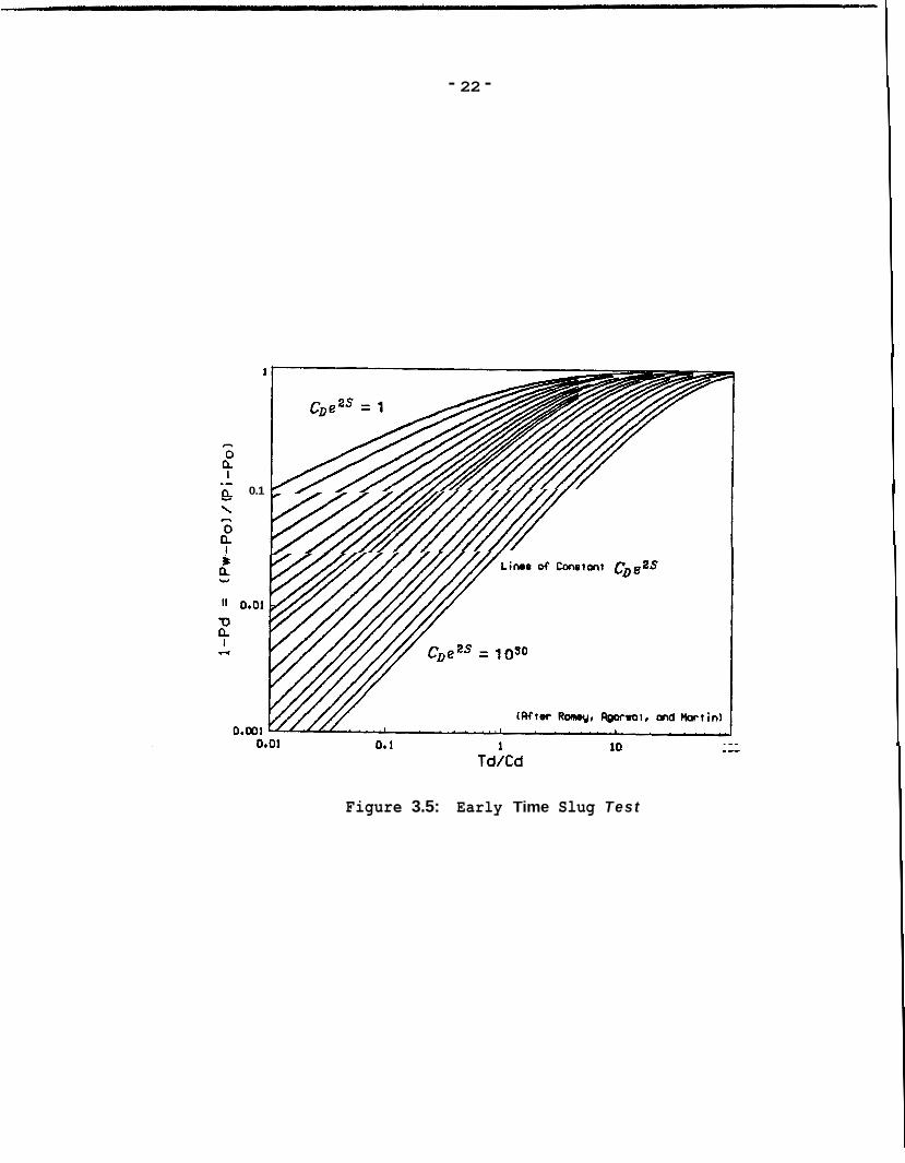
- 22 -

1

0.1

Td/Cd

Figure 3.5: Early Time Slug Test

-23-

0.g

0.E

0.7

0.6

0.5

0.4

0.3

0.2

0.1

0 0.01 0.1 1 10 100

- 2 4 -

0.1

a 0.01

II

a -0

0.001 Rtlor Romey. FrgorwoI, and Morrin)

0.01 0.1 1 10 100 1000 Y

Td/Cd

Figure 3.7: Late Time Slug Test

~~~ ~ ~ ~

- 2 6 -

Closed Chamber Test

Using the model developed in Section 3.4, closed chamber pressure response

data can be generated for a wide variety of reservoir parameters and tool confi-

gurations. Because the closed chamber test is similar to the slug test, plotting

closed chamber response data on the slug test coordinates is a logical extension

of the type curve technique. Closed chamber field data could then be analyzed by

type curve analysis, as shown to be effective for the slug test. But, as the sensi-

tivity study presented in Section 6 indicates, closed chamber pressure response

data cannot be reduced to a single set of general type curves using the slug test

dimensionless groups. In order to correctly evaluate unknown transmissibility and

skin effect, it is therefore important to understand the influence of each reservoir

end tool parameter on the dimensionless plots.

For the closed chamber test, dimensionless pressure is not a function of only

Initial CDeZs and t D / C’ because CD is not constant throughout the test.

Perhaps if C’ were evaluated at every pressure point the curves could be col-

lapsed. But such an analysis would not be practical for evaluating field data.

When C’ is evaluated using initial chamber pressure, variables such as initial

chamber pressure and initial fluid height separate curves of equal skin effect.

Thus there is no particular utility in choosing t ~ / CD as the abscissa.

Yet type curve matching is still an effective means t o match the model

parameters to actual field data. For a given set of tool parameters and estimated

reservoir properties, the pressure response can be generated using the model and

graphed in dimensionless p~ versus t D format. The resulting dimensionless curve is

independent of the assumed permeability. Type curve matching of field data can

therefore be used to calculate field permeability from the time match, and skin ef-

fect from the curve shape.

- 26 -

The optimum dimensionless format for the closed chamber type curve would

emphasize the influence of skin effect on curve shape, and minimize the effect of

tool geometry. The greater the effect of skin effect on curve shape, the greater

will be the resolution of the type curve when determining the wellbore skin effect.

Using the traditional definition of t~ for the abscissa will eliminate the effect of

other reservoir parameters, with the exception of sand thickness.

In order to determine which of the three slug test type curve formats would

yield the greatest resolution to skin effect, pressure responses were generated

for skin effect values of 0 to +8. The reservoir and tool parameters used in the

superposition model are given in Table 6.1. Similar to the slug test formulation,

negative values of skin must be represented by effective well bore radius.

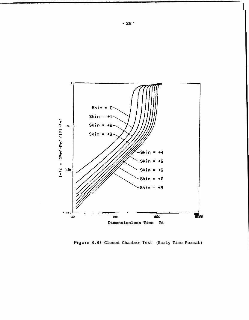
Figures 3.8, 3.0, and 3.1 0 are dimensionless plots of the simulated pressure

responses. Inspection of these three plots suggest that the late time format

yields the greatest resolution to skin effect. When transmisslbility Is also an unk-

nown, the time match would make it difficult to match the curve shape in Figures

3.8, and 3.0 because the curves are nearly similar in shape. It is therefore recom-

mended that the late time format be used for the type curve match.

3.8 Typical Response

To better understand the closed chamber well test response, the time depen-

dence of the variables was studied. Reservoir and tool parameters used in the

closed chamber superposition model to generate the followlng plots are given in

Table 6.1.

Figure 3.1 1 Illustrates how the fluid level rise occurs when the lower surge

valve opens. Note that within 20 seconds the chamber is almost entirely filled

with liquid. After 20 seconds the flow rate is essentially zero because a very

small addition of fluid to the chamber results in a large gas pressure rise.

- 27 -

Figure 3.1 2 illustrates the rise in chamber gas pressure as the gas is isother-

mally compressed. The chamber gas pressure is responsible for the abrupt rise in

the bottom hole flowing pressure. Fluid influx causes separation of the chamber

pressure curve from the bottom hole pressure. In the absence of momentum and

friction, the difference in the two curves is the hydrostatic pressure differential

of the fluid column.

Figure 3.1 3 confirms that for the moderate reservoir pressure and tempera-

ture of table 6.1, the gas compressibility factor of the chamber gas does not sig-

nificantly deviate from unity. This is expected at the moderate range of pseudo

reduced temperature. For a reservoir temperature of 175 (F) the pseudo reduced

temperature of the gas is approximately 1.7 for a hydrocarbon gas of 0.65 specif-

ic gravity relative to air.

- 28 -

1 -

51 -

1 -

I I

10 100 lo00 1 OOOO

Dimensionless Time Td 10

d . . . . . , , I

1 0 0 lo00

Dimensionless Time Td 1 OOOO

Figure 3.88 Closed Chamber Test (Early Time Format)

- 29 -

1

0. e

0.8

0.7

0.6

0.5

0.4

0.3

0.2 '

0.1 .

t

Skin = 0 1

Skin = + I /

Skin = +2/

Skin = +3/

/

/

/

Skin = +4 4

\

~ S k i n = +5 c

/Skin = +6

/-Skin = +7 I

/-Skin = +8

Dimensionless Time Td

Figure 3.98 Closed Chamber Test (tliddte Time Format)

- 30 -

0.1

0.01

Skin = +2 A

Sk

vSkin = +3 1 Skin

#

Skin #

Skin /

/Skin

(skin

+4

+5

+6

+?

+8

100 1000 loo00

Dimensionless Time Td

Figure 3.10: Closed Chamber Test [Late Time Format)

- 3 1 -

Figure 3.11 Fluid Level vs Time for Bosecose

5000 L

Pch

-

10 20 30 40 50 60 70 80 00 I00

- 32 -

1

0.88

0.96 -

0.04 -

0.82 -

0.8 -

0.88 -

0.86 -

0.84 -

0.82 -

0 10 20 30 4 0 50 60 70 80 90 100

T I E ISECONDSI

Figure 3.13 Chamber Cos Deviation Factor vs Time f o r Basecase

- 33 - 4: VERIFICATION OF CLOSED CHAMBER MODEL

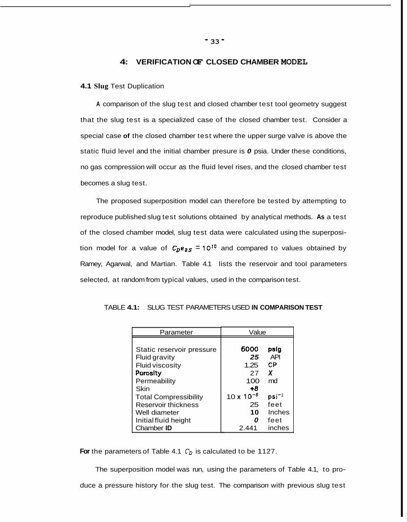
4.1 Slug Test Duplication

A comparison of the slug test and closed chamber test tool geometry suggest

that the slug test is a specialized case of the closed chamber test. Consider a

special case of the closed chamber test where the upper surge valve is above the

static fluid level and the initial chamber presure is 0 psia. Under these conditions,

no gas compression will occur as the fluid level rises, and the closed chamber test

becomes a slug test.

The proposed superposition model can therefore be tested by attempting to

reproduce published slug test solutions obtained by analytical methods. As a test

of the closed chamber model, slug test data were calculated using the superposi-

tion model for a value of CDe,, = 10" and compared to values obtained by

Ramey, Agarwal, and Martian. Table 4.1 lists the reservoir and tool parameters

selected, at random from typical values, used in the comparison test.

TABLE 4.1: SLUG TEST PARAMETERS USED IN COMPARISON TEST

Parameter

Static reservoir pressure Fluid gravity Fluid viscosity Poroslty Permeability Skin Total Compressibility Reservoir thickness Well diameter Initial fluid height Chamber ID

Value

6000 25

1.25 27

100 +8

10 x 10 -6 25 10 0

2.441

Psig API

CP x md

psi-' feet Inches feet inches

For the parameters of Table 4.1 C' is calculated to be 1 127.

The superposition model was run, using the parameters of Table 4.1, to pro-

duce a pressure history for the slug test. The comparison with previous slug test

1

- 3 4 -

solutions required calculation of dimensionless variables. Table 4.2 presents the

comparison.

TABLE 4.2: COMPARISON OF SUPERPOSITION CALCULATED SLUG TEST

2.00 5.00

10.00 20.00

Superposition

PD

0.990376 0.981 496 0.9561 87 0.9 16555 0.845057 0.668265 0.459848 0.22746 1

Analytic

P D

~~ ~

0.990324 0.981 367 0.955945 0.91 6404 0.844376 0.667704 0.458279 0.226036

Difference

( X )

~~~ ~

0.005 0.01 3 0.025 0.01 6 0.081 0.084 0.342 0.628

And the analytic values are those of Ramey, Agarwal, and Martin (1 976).

Comparison of slug test data, obtained using the superposition model, with

published results, indicate the proposed model accurately duplicates Ramey's

results obtained by numerical approximation of the integral solution to the slug

test. Close agreement is expected because many of the assumptions of the slug

test solution, including negligible friction and momentum effects, are also included

in the superposition model.

The comparison supports the proposed superposition model but does not veri-

fy correct pressure response generation in the presence of compressing chamber

gas. Yet the ability to generate slug test data, indicates correct modeling of

reservoir behavior in the superposition model. The gas chamber pressure calcula-

tion is a simple addition as shown in Section 3.4.

1

-35-

4.2 Closed Chamber Variance from Slug Test

The influence of the upper surge valve on the pressure response can be illus-

trated by comparison with the superposition results of Section 4.1. The superpo-

sltion model was used to generate a pressure response for the parameters of

Table 4.1 with the addition of an upper surge valve. A chamber length of 3000

(ft) and an initial chamber pressure of 14.7 (psia) were selected.

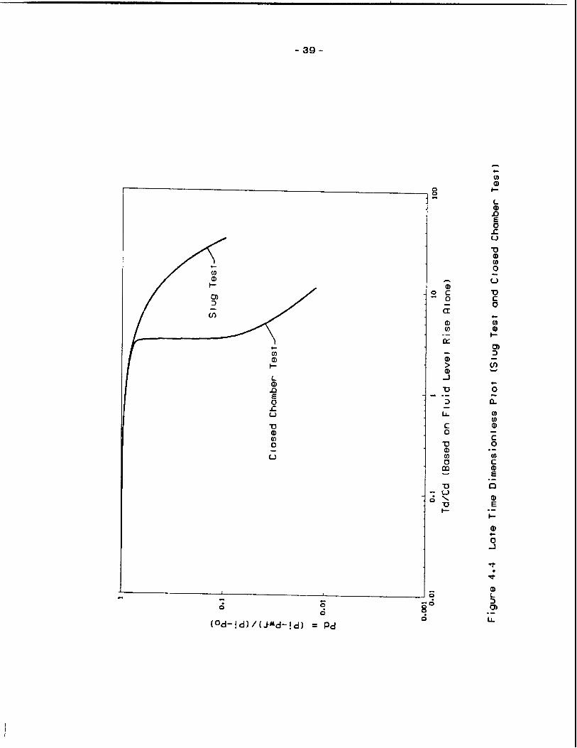
Figure 4.1 shows the pressure response for both the slug and closed chamber

test. Figures 4.2, 4.3, and 4.4 show the dimensionless comparison of the slug and

closed chamber tests.

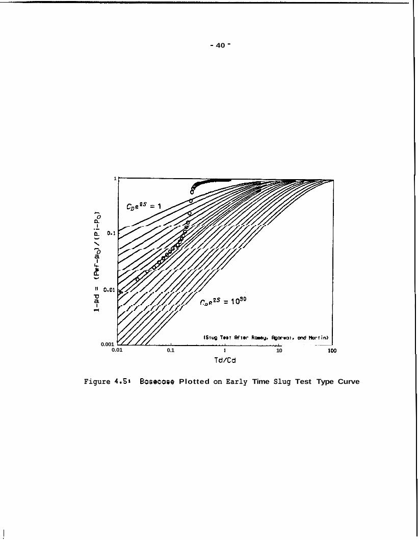
Figures 4.5, 4.6, and 4.7 show the dimensionless basecase response plotted

on the slug test type curves of Ramey, Agarwal, and Martin (1 975). Initially, the

basecase behaves as a slug test, because at early time the chamber gas pres-

sure does not rise significantly and the well bore storage is nearly constant. As

the fluid level nears the upper surge valve, an abrupt change in storage occurs.

The late time response again resembles a slug test but is shifted in time due to

the decreased value of well bore storage governed by the chamber gas pressure.

On logarlthmic coordinates the shift in time of the late time response is proportion-

al to the ratio of the initial to final well bore storage.

(UISd) 3tlnSS3tld 310H WO1108

-37-

0 0 C

e

.- cn C

- 38 -

I

0.0

0.8

0.7

0.6

0.5

0.4

0.3

0.2

0.1

0

Closed Chamber Test

1

Test

0. I I 10 100

Td/Cd (Based on Fluid Level Rise Fllone)

Figure 4.3 Middle Time Dimensionless Plot (Slug Test ond Closed Chomber Test)

-39-

al E

- 40 -

1

tL 0 I

a 0 c I L

U a I

0.001 0.01 0.1 1 10

Td/Cd

Figure 4.58 Bosecase Plotted on Early Time Slug Test Type Curve

- 4 1 -

0.01 0.1 1 10

Td/Cd

Figure 4.6: Bosecose Plotted on Middle Time Slug Test Type Curve

- 42 -

1

0. I

6.01

100 lo00

Td/Cd

igure 4.78 Bosecose Plotted on Late Time Slug Test Type Curve

I

- 43 -

5: NUMERICAL CONSIDERATIONS

6.1 Time Step Selection

As noted in the preceding section, the closed chamber test response is

equivalent to the slug test response until the chamber gas pressure becomes sig-

nificant compared t o the static reservoir pressure. When the chamber gas pres-

sure begins to effect the response, the bottom hole pressure rise is much more

rapid. Numerical modeling of the closed chamber test requires selection of a time

step size sufficiently small that the chamber pressure rise is accurately

represented. The rate at which the pressure rise occurs is dependent upon the

Initial chamber pressure, and the geometry which defines the relationship between

fluid influx and compression ratio of the chamber gas.

Momentarily assume that the chamber gas behaves as an ideal gas. Also

assume that the chamber gas compression is isothermal. Under these assump-

tions, the chamber gas pressure Is equal to the initial chamber pressure times the

volumetric compression ratio of the closed chamber. If the initial chamber pressure

is small compared to the initial reservoir, as is often common when the initial

chamber pressure is near atmospheric pressure, the chamber pressure will only

approach the reservoir pressure when the volumetric compression ratio is very

large. Simply stated, for a low initial chamber pressure, the chamber pressure will

only effect the rate of influx when the fluid level is very near the upper surge

valve.

Numerical problems occur if the time step size causes the fluid level to vary

- 44 -

excessively during one time step. When the time step is excessive, the effect is

to cause the numerical model to over shoot the upper surge valve. This occurs

because the model calculates the fluid influx during a time step assuming constant

bottom hole pressure, as illustrated in Figure 3.3. A forward looking routine is

required to extend the calculation one step past the pressure history. The bottom

hole pressure used during a time step was calculated using the chamber pressure

at the end of the previous time increment. If at the beginning of the time step the

fluid level is significantly below the upper surge valve, the assumption of constant

bottom hole pressure during the time increment may cause calculation of fluid

influx resulting in a fluid level at the end of the time step which is above the

upper valve. All subsequent chamber pressure calculations will calculate a nega-

tive value using Equation 3.22, and the fluid level rise will never feel the resis-

tance of the gas compression.

Assuming isothermal, ideal gas compression, a simple estimate may be made of

the maximum permissible time step. For an ideal gas, Equation 3.22 may be written

as:

To avoid fluid level over shoot of the upper surge valve, the maximum change in X

per time step should not exceed the chamber volume at which the chamber pres-

sure is sufficient to resist fluid influx. Neglecting the hydrostatic pressure dif-

ferential of the fluid column, this occurs when the chamber pressure is equal to

the initial static reservoir pressure. With these assumptions the following expres-

sion may be written:

- 4 5 -

Using dimensionless influx, AX, can be related to time. For conservative

estimation of the maximum permissible time step, assume the bottom hole pressure

is equal to the initial chamber pressure after the lower surge valve opens. This

assumption is consistent with neglecting the hydrostatic pressure differential of

the liquid column. With this assumption Equation 3.19 may be written to give the

influx during a single time step:

For e single time step Equation 3.23 may be written as:

N AX, = Ah

Substituting Equation 5.3 into equation 5.4 yields:

Then equating Equations 6.2 and 5.5 and rearranging to solve for maximum dimen-

sionless influx during a single time step:

After calculating the maximum allowable value of dimensionless influx during a

single time step, the maximum permissible value of AtD can be determined from

tabulated values of QD for skin equals zero. As with other assumptions used in

this development, using skin equals zero tables of dimensionless influx will result in

e conservative value of the maximum time step. The maximum permissible time

step is finally obtained from the dimensionless time step:

- 46 -

Where At- is expressed in seconds and k, is the maximum expected average

reservoir permeability expressed in millidarcys.

- 47 -

6.2 Improvements in Efficiency of Time Step

The time step requirements discussed in the preceding section often result in

use of an extremely small time step. For example the sensitivity study examples

presented in the next section required a time step of 0.01 seconds to avoid over

shoot of the upper surge valve. When pressure data is desired over a reasonable

interval of time the superposition routine can require unreasonable amounts of

computer time. To obtain 100 seconds of pressure data for the sensitivity study,

of Section 6, about one hour of run time was required on the Petroleum Engineering

department’s VAX 1 1 /750 computer.

The period during which a small time step is required is only a fraction of the

total test duration. To increase the efficiency of the superposition routine a

scheme could be developed utilizing a variable time step. This would allow use of

e larger time increment during the flow period when the chamber pressure is insig-

nificant compared to reservoir pressure. As the fluid level approaches the upper

surge valve the time step would have to be reduced to avoid over shoot of the

upper surge valve. After the chamber pressure increases to near the reservoir

pressure, the time step could be increased to a larger value again because the

rate of pressure change with respect t o time becomes small as the flow rate de-

creases. Time step size could be controlled by monitoring the derivative of

chamber pressure with respect ot time and maintaining the rate of pressure

change below some preset value.

The amount of numerical calculation could be greatly reduced by such a

scheme. The reduction is much greater than proportional to the number of time in-

crements deleted, because at each time step the superposition routine requires

subtraction of all previous pressure changes. A variable time step model could in-

crease the efficiency of the superposition model by an order of magnitude.

- 48 -

Evaluation of cumulative fluid influx a t a point in time by superposition re-

quires that the dimensionless influx be evaluated for all combinations of the previ-

ous time steps. Thus if the time step is allowed to vary continuously new dimen-

sionless influx values would have to be calculated for each pressure change in the

entire pressure history, at every time step. This requirement would negate the

benefit of varying the time increment size.

The recalculation requirement can be circumvented if all time steps are a mul-

tiple of some small basic unit of time. The basic unit of time increment should be

equal to the maximum permissible time step during the period of rapid chamber

pressure rise as predicted by Equation 5.7. By utilizing a multiple time step incre-

ment the amount of superposition required could be significantly reduced without

the need to recalculate dimensionless influx values at each time step. The only

additional required calculation, over the constant time step model, would be the

need to keep a record of the cumulative time each pressure change has been in

effect and update the record at each time increment.

Although a variable time step superposition model is not presented in this re-

port, a simple model was developed and shown to produce pressure response data

much more efficiently than the constant time increment model presented. Many

problems were encountered in developing a method of adjusting the number of time

increments per time step. When the time step size was not reduced quickly

enough, as the fluid level neared the upper surge valve, the model became un-

stable and produced oscillating pressure values. Continued development of a vari-

able time step superposition model will be necessary to quickly generate closed

chamber well test type curves as needed to analyze field data.

1

- 4 9 -

6: SENSITIVITY STUDY

General Description

Plotting of the closed chamber pressure response on slug test dimensionless

coordinates indicates that many tool and reservoir parameters influence the

dimensionless curve shape. The influence of tool and reservoir parameters should

be understood, if traditional slug test type curve format is to be used in closed

chamber test analysis. Such information is needed to predict the accuracy of

measurement required to define a closed chamber test. Furthermore, knowledge of

the influence of each input parameter will facilitate choosing realistic assumptions

for future analytic approaches to the closed chamber test solution. Many of the

tool parameters can be selected for a particular test situation. Knowing the infiu-

ence of each tool parameter would allow the tool assembly to be designed for

maximum sensitivity to unknown reservoir parameters.

Input Parameter sensitivity was therefore investigated using the superposi-

tion closed chamber computer model. Isolation of each parameter was obtained by

creating a control basecase. Sensitivity analysis was then performed by varying a

single parameter over a typical range. The basecase values were selected at ran-

dom from what are believed to be typical values. Table 6.1 lists the basecase

parameters.

- 60 -

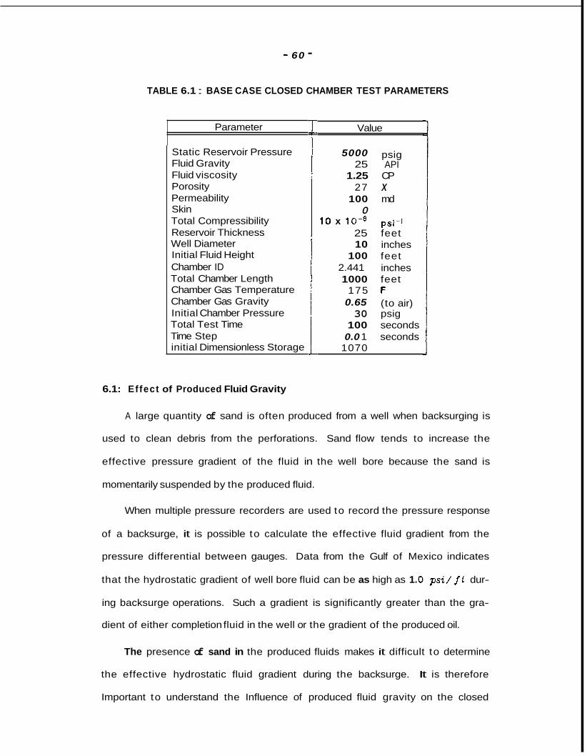
TABLE 6.1 : BASE CASE CLOSED CHAMBER TEST PARAMETERS

Parameter

Static Reservoir Pressure Fluid Gravity Fluid viscosity Porosity Permeability Skin Total Compressibility Reservoir Thickness Well Diameter Initial Fluid Height Chamber ID Total Chamber Length Chamber Gas Temperature Chamber Gas Gravity Initial Chamber Pressure Total Test Time Time Step initial Dimensionless Storage

Value

5000 psig 25 API

1.25 CP 27 X

100 md 0

10 x 10-8 psi-' 25 feet 10 inches

100 feet 2.441 inches 1000 feet

175 F 0.65 (to air) 30 psig

100 seconds 0.0 1 seconds

1070

6.1: Ef fect of Produced Fluid Gravity

A large quantity of sand is often produced from a well when backsurging is

used to clean debris from the perforations. Sand flow tends to increase the

effective pressure gradient of the fluid in the well bore because the sand is

momentarily suspended by the produced fluid.

When multiple pressure recorders are used to record the pressure response

of a backsurge, it is possible to calculate the effective fluid gradient from the

pressure differential between gauges. Data from the Gulf of Mexico indicates

that the hydrostatic gradient of well bore fluid can be as high as 1 .O ps i / f t dur-

ing backsurge operations. Such a gradient is significantly greater than the gra-

dient of either completion fluid in the well or the gradient of the produced oil.

The presence of sand in the produced fluids makes it difficult to determine

the effective hydrostatic fluid gradient during the backsurge. It is therefore

Important to understand the Influence of produced fluid gravity on the closed

- 51 -

chamber well test response.

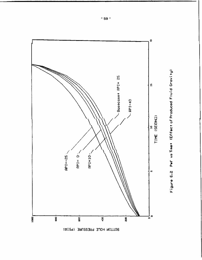
Produced fluid gravity was varied from -25 to 40 degrees API. Table 6.2

presents the pressure gradient of the fluid densities tested.

TABLE 6.2: FLUID GRADIENTS OF DENSITIES TESTED

API Gravity I Ibm/gal psi/ft

40

0,433 8.34 10 0.391 7.54 25 0.375 6.88

0 8.97 0.466 -25 11.08 0.575

Figure 6.1 presents the pressure response data generated using the super-

position model. Figure 6.2 is an enlargement of Figure 6.1 which emphasizes the

influence of fluid gravity. As expected the pressure rise is more abrupt for heaver

fluid.

Figure 6.3 presents the early time dimensionless plot of the pressure data.

Fluid gravity causes a change in the early time curve shape. Comparison of Figure

6.3 and Figure 3.5 indicates confusion may occur if the early time format were to

be used for type curve skin determination when the produced fluid gravity is also

unknown.

Figure 6.4 illustrates that fluid gravity variation has little effect on the late

time dimensionless plot. It is therefore not necessary to accurately measure the

produced fluid gravity if the late time curve is used for the type curve analysis of

field data. This is also expected because the late time pressure rise Is governed

by the gas compression.

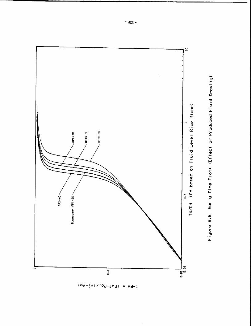
Figures 6.5 and 6.6 are included to illustrate that using tD / CD as the

abscissa to collapse the dimensionless curves is ineffective. Practical use of the

type curve technique of history matching requires that to be divided by a

- 62 -

constant value of CD. Division of dimensionless time by the changing value of

dimensionless well bore storage may collapse the curves, but the resulting graph

would be useless for field data evaluation.

In Figure 6.5 fD is divided by dimensionless well bore storage calculated from

well bore storage resulting from the rising fluid level alone. Note that this plot is

successful in collapsing the early time response. During this period the effect of

gas compression is not significant, and the response is equivalent to a slug test.

But as expected, at late time, when the gas compression becomes important, the

curves separate due to the changing value of well bore storage.

Figure 6.6 illustrates that including storage due to initial gas compression in

the constant value of CD by which tD is divided does not improve the curve col-

lapsing effect of using t ~ / CD as the abscissa.

6.2: Effect of Chamber Gas Gravity

The basecase gas gravity was varied from 0.5 to 1.6 (relative to air) to test

the influence of chamber gas gravity on the closed chamber well test pressure

response. Figure 6.7 illustrates that gas gravity does ot significantly effect the

Isothermal pressure response.

6.3: Effect of Initial Fluid Level

Well bore storage resulting from a rising fluid level is dependent upon the

cross sectional area of the liquid interface and the density of the well bore liquid.

As a result, the slug test dimensionless response is independent of the initial fluid

level. To investigate the significance of initial fluid level on the closed chamber

response, the basecase initial fluid level of 100 ft was varied between 0 and 500

ft.

Figure 6.8 illustrates how initial fluid level influences the pressure versus

time plot. Figures 6.9 and 6.10 illustrate that the influence of fluid level on the

- 53 - dimensionless plots is more significant in the late time data. Both Figures 6.9 and

6.1 0 indicate that a smaller initial chamber gas volume, due to a longer initial fluid

column, results in an earlier rise in the chamber pressure. If slug test type curves

were to be used to evaluate a closed chamber well test, a lower initial fluid level

would result in a greater portion of the data matching with the early time slug test

type curve.

To further illustrate the ineffectiveness of using tD/ CD as the abscissa,

when CD is a function of fluid level rise only, Figures 6.1 1 and 6.12 are included.

Note that as the initial fluid column length is increased the curves separate earlier.

This is because the well bore storage change occurs earlier due to the chamber

pressure rise which is a result of the smaller initial gas volume. Less fluid influx is

required before the volumetric compression ratio of the gas governs the bottom

hole pressure response.

6.4: Effect of initial Chamber Pressure

The initial gas pressure in a closed chamber test is usually ambient atmos-

pheric pressure. If either a tool joint or one of the surge valves leaks during the

run in of the test assembly the fluid level inside the chamber may rise resulting in

premature compression of the chamber gas. It is therefore Important to under-

stand the influence of initial chamber pressure.

Figure 6.13 shows how a higher initial chamber pressure tends to smooth the

pressure response. This is expected because less compression of the gas is

required before the gas pressure governs the bottom hole pressure.

Figure 6.14 illustrates that increasing the initial chamber pressure shifts the

early time dimensionless plot to the left and causes an earlier increase in

(1 - p D ) . If slug test type curves were to be used to evaluate the early time

closed chamber response an initial atmospheric chamber pressure should be main-

- 64 -

tained. Even a chamber pressure of 30 psig causes a time shift to the left that

would cause permeability determined by the slug test type curve match point to

be artificially low.

Figure 6.1 5 indicates that the late time format of data plotting is not as sig-

nificantly influenced by the initial chamber pressure. As with Figures 6.1 3 and

6.1 4 the response is smoothed by an increase in chamber pressure, but no signifi-

cant time shift occurs.

Figures 6.1 6 and 6.1 7 illustrate these points on traditional slug test coordi-

nates. But as with the other cases presented, the closed chamber curves cannot

be reduced to a single type curve by plotting on slug test coordinates.

6.5: Ef fect of Total Chamber Length

When well control problems are anticipated, safety dictates that the upper

surge valve be placed deep enough that if the chamber pipe should part and

create an upward piston action the tool assembly remain heavy. This requirement

often limits the chamber length which can be used to surge shallow high pressure

sands. To Investigate the effect of total chamber length the basecase length of

1000 ft as varied to 500 and 2000 ft.

Figure 6.1 8 indicates that the abrupt pressure rise due to chamber gas

compression can be delayed by utilizing a longer chamber. This idea is supported

by Figure 6.19 which shows that a longer chamber results in more of the response

being similar to the slug test. This effect is also expected because a slug test

can be thought of as a closed chamber test with an infinite chamber length.

Figure 6.20 illustrates that the late time format response is also delayed by

use of a longer chamber. Such a delay would allow pressure recording with a less

accurate device. Closed chamber tests are usually of such short duration that

traditional mechanical pressure recorders lack sufficient sensitivity to record the

-55-

true pressure response. Thus it appears beneficial to use as long of chamber

length as possible.

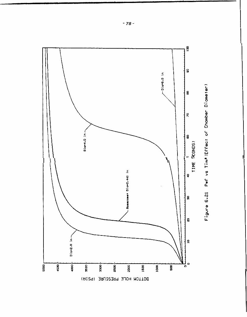
6.6: Effect of Chamber Diameter

A similar effect can be obtained by increasing the chamber diameter. This

increases the portion of well bore storage attributable to the rising fluid level.

More fluid influx is required before the gas compression becomes significant,

resulting in a time shift to the right. Because the flow period is longer a larger por-

tion of the formation is investigated.

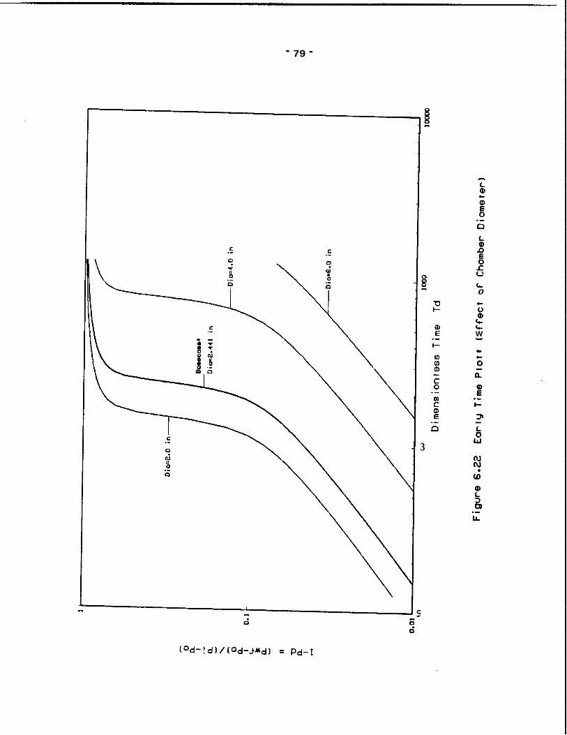
Figure 6.21 shows how the abrupt pressure rise is delayed by increasing the

chamber diameter. Figure 6.22 and 6.23 illustrate the dimensionless time shift to

the right caused by increasing the internal tool diameter.

Analogous to the tool length increase, an Increase in chamber diameter would

decrease the pressure recorder sensitivity required to accurately record the

closed chamber pressure response. But unlike increasing the chamber length,

increasing the chamber diameter does not decrease the safety of the test.

6.7: Effect of Reservoir Sand Thickness

Reservoir sand thickness also causes a time shift in the dimensionless plots.

A thicker sand increases the ability of the formation to quickly fill the chamber.

Early chamber gas compression occurs as a result, and the abrubt rise in the bot-

tom hole pressure occurs sooner.

Figure 6.24 shows the influence of reservoir sand thickness on the pressure

versus time plot. Figure 6.25 and 6.26 illustrate the time shift which occurs on

dimensionless coordinates.

Type curve generation by the superposition model requires estimation of the

reservoir sand thickness. Dimensionless time does not contain sand thickness so

the time match of field data will yield only (-1 . But because the dimensionless k P

- 66 -

curves shift with respect to time as sand thickness varies the same transmissibil-

ity, (-), should result from the field data match regardless of the initial sand

thickness estimate. This occurs because reservoirs of equal transmissibility will

yield equivalent pressure responses, if all other parameters are equal.

kh rcL

6.8: Effect of Initial Reservoir Pressure

The flow period of a closed chamber test is usually of very short duration. As

a result the bottom hole pressure of the well quickly returns to the Initial static

reservoir pressure. If the tool assembly is not quicklypemoved from the well a

good estimation of static reservoir pressure is obtained from the final pressure

recording prior to release of the temporary packer. Yet unlike the slug test

response, the closed chamber dimensionless plots are effected by the reservoir

pressure.

Figure 6.27 illustrates how initial reservoir pressure effects the pressure vs

time response. The increase in the final pressure trend of the closed chamber

test response is expected. Also note that the period of rapid pressure rise due to

gas compression occurs earlier for higher pressured formations. This occurs as a

result of the increased flow rate due to greater pressure differential at the sand

face.

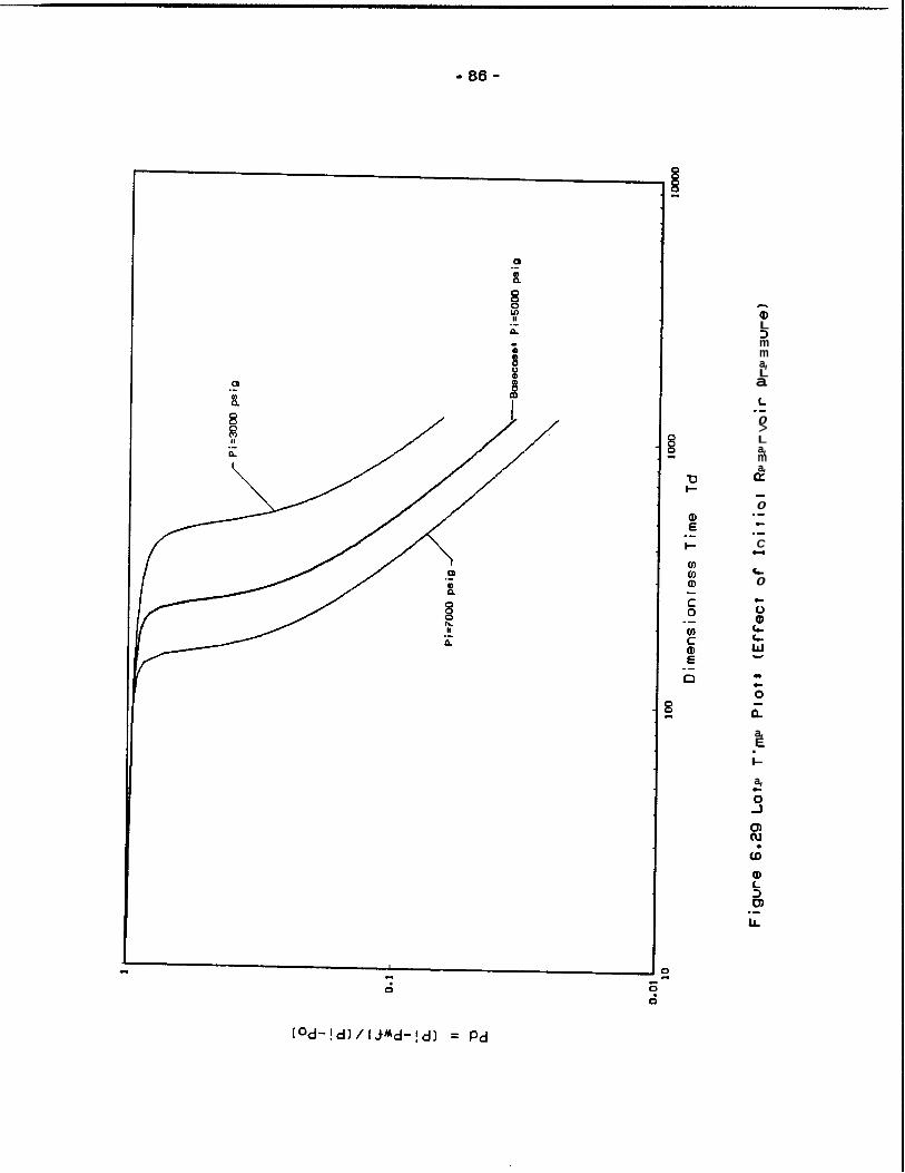
Figure 6.28 again illustrates a difference between slug and closed chamber

tests. A t very early time, when the closed chamber test behaves as a slug test,

initial reservoir pressure does not influence the dimensionless plot. But at latter

time the influence of initial reservoir pressure becomes significant as emphasised

in Figure 6.29.

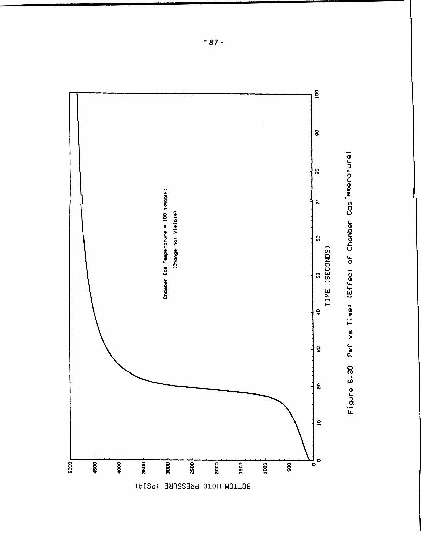
6.9: Effect of Chamber Gas Temperature

As discussed in Section 3.4, the thermodynamic path of gas compression is

not known. To simplify the mathematical model isothermal gas compression was

- 57 -

assumed. Figure 6.30 illustrates that the temperature at which the isothermal

gas compression occurs does not influence the pressure response. If the gas

compression occurs adiabatically the gas temperature will increase as the pres-

sure increases. Based on the results of Figure 6.30, it is probable that adiabatic

gas compression will not significantly alter the isothermal bottom hole pressure

response. Further studies should confirm this concept.

6.10: Effect of Assuming Ideal Gas Behavior

An assumption of ideal gas behavior would greatly simplify the partial dif-

ferential equations which govern the closed chamber pressure response. To

investigate the error induced by assuming ideal gas behavior the superposition

model was modified with the gas deviation factor set equal to unity.

Figure 6.31 illustrates that for the typical reservoir temperature and pressure

values of the basecase, the assumption of ideal gas behavior does not effect the

pressure response. For reservoir pressures approaching 10,000 psig the affect

may be more significant.

(UISdl 3tlflSS3tid 310H Roll08

- 59 -

I

c. 0

c


- 80 -

> 0

u L

0 0

I- U

D 8 0 3

c B a c 0 c

8 E

L

W 0

8 L

D 3

- e1 -

0 >

0 c

c 0

t

- 62 -

- 63 -

- 64 -

Y

(UISdl 3UnSS3Ud 310H NO1108

c 0 c 0

c a, c W - a a, E .- I-

v) >

(UISd) 3tlflSS3ltld 310H WO1108

i

b w

- 6 7 -

0

c Q,

0 d

c c

C C

U C

LL

c c

8 - II

-I .-

c L

c rr

I

D .-

(UISd) 3UnSS3Ud 310H WO1108

- 71 -

I C

L

L a,

E 0

u L

n

0 .- e .- C

a, E .- I-

a,

-I 0 c

- 73 -

- 74 -

c

' I

' c 0 _- a, a,

(D c a 0 E 0

a, c3 0

c 0 c

a c 0 - a

c O w

- 76 -

(UISd) 3tlnSS3tld 310H HOllO8

I \

I c c

\ \

- 77 -

c 0 0

c

E 4

0

C a, .J

L a,

0 E

0 f

n

a, E

I- .-

0 cu

- 78 -

\

(UISdl 3tlflSS3ad 310H WO1108

- 79 -

3

c 0,

c 0 c

c W

- 80 -

L @ c 6 0 E

c 0 c

6 E

@

J 0 c

- 81 -

(UISd) 3tlnSS3tld 310H I401108

- 02 -

fn fn

Q E

- 83 -

c c

% 2: 0

0

m x A

u) u) 8 C Y 0

W C

co 0

c 0 c

8 E .-

- 84 -

0

(UISd) 3klflSS3tld 310H WOllOB

- 85 -

\

i

J

c. - d

U C

Q) E .-

L 0 w

L 3 m m a, L a .- L

0 > L a, m a, e

0 - .- .- c U C

c 0 c

a, E .- I-

a,

- 87 -

0 Y) 0


- 88 -

C

a

(UISdl 3tlnSS3tld 310H WO1108

- 89 -

7: CONCLUSIONS AND RECOMMENDATIONS

A computer model was developed to simulate the pressure response of a

closed chamber well test. Superposition of the constant pressure, cumulative

influx solution to the radial diffusivity equation was used in the model to avoid the

direct solution of the governing non-linear partial differential equations. Although

real gas compressibility effects were included in the model, the effects of friction

and momentum were not. Chamber gas compression was assumed isothermal in the

mathematical model development.

The proposed superposition model was tested for ability t o reproduce the

slug test solution of Ramey, Agarwal, and Martin (1875). Agreement was found to

be within 0.7 X for values of t D / CD less than 20. The percent deviation was

shown to increase with respect to t,/ CD. The deviation is believed a result of

the cumulative error present in both solutions.

The superposition model provided illustration of differences between the slug

test and closed chamber test. Initially the closed chamber test behaves as a slug

test. Compression of the chamber gas causes the well bore storage to decrease

during the test resulting in a dimensionless curve change on the slug test coordi-

nates of Ramey et. al.. The final portion of the dimensionless curve is shifted on

logarithmic coordinates an amount proportional to the ratio or the initial to final well

bore storage. Because well bore storage changes during the test, there is no

advantage to using t ~ / CD as the abscissa, as is an effective curve collapsing

technique for the slug test.

- 90 -

The superposition model was used to generate dimensionless response

curves for varying values of Hurst skin effect. The late time slug test format, with

tD as the abscissa, yields the greatest resolution to skin.

A sensitivity study was conducted to evaluate the influence of nine reservoir

and tool parameters on the closed chamber pressure response. For a reservoir

pressure of 5000 psig the effect of non-ideal gas behavior was shown insignifi-

cant. As a result, the pressure response is independent of gas gravity. Chamber

gas temperature also was shown to have little effect on the bottom hole pressure

response of the closed chamber test. In addition to yielding the greatest resolu-

tion to skin effect, the late time format of dimensionless plot was shown to be the

least influenced by produced fluid gravity, which is often not known.

A greater portion of the closed chamber test response was shown to behave

as a slug test as the chamber length and chamber diameter are increased. Simi-

larly, maintaining an lnltial chamber pressure near atmospheric is required to pro-

duce slug test behavior during the early portion of the closed chamber test. Thus

proper test tool design would allow a greater portion of the closed chamber test

response to be analyzed using the slug test type curves of Ramey, Agarwal, and

Martin (1 975).

The results of the sensitivity study indicate that many variables, such as ini-

tial fluid column length, influence the closed chamber test pressure response.

Because the solution approach was not analytic the dimensionless groups required

to generalize the closed chamber test response were not derived. But the similar

effect of chamber diameter and reservoir sand thickness suggest the existence

of such groups.

Generation of closed chamber type curves for a particular test situation, by

the superposition model, will require improvements in the efficiency of the model.

An algorithm utilizing a variable time step composed of multiple increments of a

- 91 -

basic unit of time is suggested. Such a routine may require an iterative pressure

calculation. It is believed that the improved model would require an order of mag-

nitude less computer time due to the repetitive nature of the superposition calcu-

lation.

The greatest contribution of the model developed is the creation of a founda-

tion for future analytic approaches to the closed chamber governing partial dif-

ferential equations. The sensitivity study has shown that for typical reservoir

pressures the chamber gas deviation from real gas behavior can be neglected.

This result should facilitate development of the dimensionless groups needed to

generalize the closed chamber test response.

Future studies should consider the effect of adiabatic chamber gas compres-

sion. Momentum and friction effects need also to be considered in the model. Data

from backsurges performed in the Gulf of Mexico indicate limited occurrence of an

oscillating fluid level resulting form the effects of momentum and friction.

Summary

A Superposition model was developed for the closed chamber test which

neglects momentum and friction but includes real gas behavior.

The superposition model is capable of reproducing the slug test results of

Ramey, Agarwal, and Martin (1 9751, which also neglected momentum and fric-

tion effects.

Closed chamber test deviation from the slug test was illustrated. The shift

on logarithmic coordinates of the late time dimensionless closed chamber

pressure response is proportional to the ratio of the initial to final well bore

storage.

For the closed chamber well test, the late time slug test format of Ramey et.

al. (19751, yields the greatest resolution to skin effect. The late time format

- 92 -

also has the advantage of being the least influenced by the produced fluid

gravity, which is often unknown.

5) For moderate reservoir pressure, (5000 psig), non-ideal chamber gas

behavior does not affect the bottom hole pressure response of the closed

chamber test. As a result, chamber gas gravity is insignificant.

6) Over a range of 100 to 500 (F), the temperature a t which the isothermal

compression of the chamber gas occurs does not influence the bottom hole

pressure response of the closed chamber test.

7) A greater portion of the closed chamber test response wiii be equivalent to a

slug test, and thus suitable for slug test type curve analysis, if the effect of

the chamber gas compression is minimized during the test. The sensitivity

study indicates that increasing the chamber length, increasing the chamber

diameter, and decreasing the initial fluid column length will decrease the

effect of chamber gas compression. An initial chamber gas pressure near

atmospheric is required to avoid deviation from the equivalent early time slug

test response.

Recommendations for Future Study

1) Return to governing partial differential equations and attempt to define

dimensionless groups to generalize the closed chamber solution. The results

of this study indicate it is reasonable to assume ideal gas behavior and thus

neglect the real gas deviation factor in the deviation.

2) Improve the Superposition model with a variable time step.

3) Consider the effect of adiabatic chamber gas compression.

4) Determine the influence of momentum and friction on the closed chamber well

test.

- 93 -

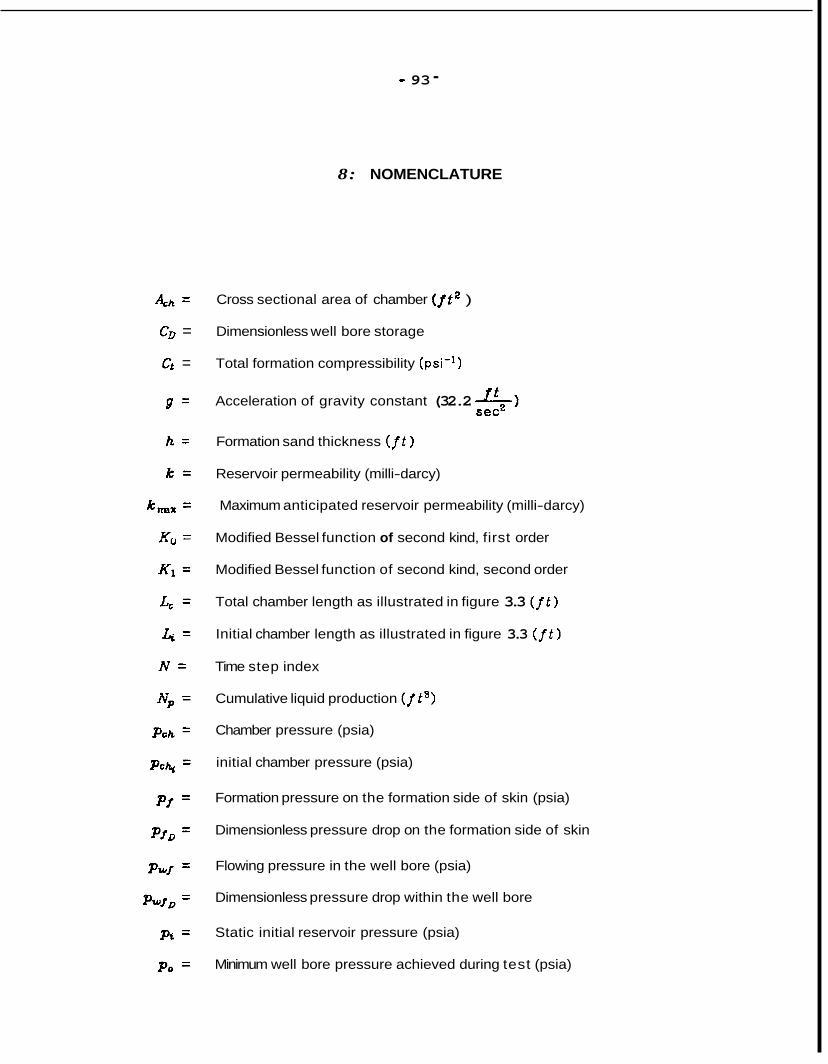
8: NOMENCLATURE

4 h =

c, =

ct =

9 =

h =

Cross sectional area of chamber ( I t 2 )

Dimensionless well bore storage

Total formation compressibility (psi-')

Acceleration of gravity constant (32.2 I t ) sec2

Formation sand thickness (ft )

Reservoir permeability (milli-darcy)

Maximum anticipated reservoir permeability (milli-darcy)

Modified Bessel function of second kind, first order

Modified Bessel function of second kind, second order

Total chamber length as illustrated in figure 3.3 (ft)

Initial chamber length as illustrated in figure 3.3 (ft)

Time step index

Cumulative liquid production ( f t s )

Chamber pressure (psia)

initial chamber pressure (psia)

Formation pressure on the formation side of skin (psia)

Dimensionless pressure drop on the formation side of skin

Flowing pressure in the well bore (psia)

Dimensionless pressure drop within the well bore

Static initial reservoir pressure (psia)

Minimum well bore pressure achieved during test (psia)

Subscripts

- 94 - Laplace Dimensionless rate of influx

Cumulative influx ( f t 9

Laplace Dimensionless cumulative influx

Dimensionless cumulative influx

Well bore radius ( f t )

Dimensionless radius

Laplace variable

Dimensionless skin factor

Time (seconds)

Time step (seconds)

Dimensionless time

Dimensionless time step

Chamber gas volume ( f t 3 )

Initial chamber gas volume ( l i s )

Dynamic fluid level as Illustrated in figure 3.3 (ft)

Fluid level change per time step ( f t )

Real gas deviation factor of chamber gas

Initial real gas deviation factor of chamber gas

Influx constant as defined in equation 3.1 7 ( f

Fluid viscosity (centi Poise)

Formation porosity (fraction)

t 3 P=

Fluid density ( -1 Lbm f t 3

ch = Chamber conditions

D = Dimensionless

- 9 5 -

o = Minimum during test

p = Produced

t = Total

zuf = Bottom hole flowing conditions

- 96 -

REFERENCES

Alexander, L. G. :"Theory and Practice of the Closed Chamber Drillstem Test Method," SOC. Pet . Eng. J . (December 1977), p. 1539.

Brill, J. P. and Beggs, H. D., University of Tulsa : "Two Phase Flow in Pipes," INTER- COMP Course, The Hague, 1974.

Dake, L. P.: Fundamentals of Reservoir Enaineerina, Elservier Scientific Publishing Company, Amsterdam, The Hague, 1974.

Da Prat, G.: "Well Test Analysis for Naturally Fractured Reservoirs," Ph.D. Disser- tation, Stanford University, July 1981.

Mateen, K.: "Slug Test Data Analysis in Reservoirs with Double Porosity Behavior," M.S. Report, Stanford University, September 1983.

Ramey, H. J., Aganval, R. G., and Martin, I.: "Analysis of Slug Test or DST Flow Period Data," Can Pet. J . (July 1975).

Saldana, M.: "Flow Phenomenon of Drill Stem Test With Inertial and Frictional Wellbore Effects," Ph.D. Dissertation, Stanford university, October 1983.

Shinohara, K.: "A Study of Inertial Effect in the Wellbore In Pressure Transient Well Testing," Ph.D. Dissertation, Stanford University, April 1980.

Stehfest, H.: "Algoritm 368, Numerical Inversion of Laplace Transforms," Commun- ications of the ACM, D-5 (January 1970) 13, No. 1 , 47-49

Standing, M. 8.: Volumetric and Phase Behavior of Oil Field Hydrocarbon Svstems , Millet the Printer, Inc., Dallas Texas 1981 , p. 122

Suman, G. O., Jr., Ellis, R. C., and Snyder, R. E.: Sand Control Handbook, Gulf Publish- ing Company, Houston Texas, 1983,30-31.

- 97 -

APPENDIX A

COMPUTER PROGRAM

- 8 8 -

C C C C C C C C C C C C C C C C C C C C C C C C C C C C C C C C C C C C C C C C C C C C C C C C C C C C C C C C C C C C C C C C

* * * * R

* I * * * * * * * * * * * * * * * * * * * * * * * * * * * * * * * R

* * * * * * * * * * * * * * * * * *

This program generates a pressure as a function of time response for a Closed Chamber D r i l l Stem test. The method of solution is a well bore material balance of the fluids produced. F l u T d influx is evaluated b y superposition of the constant pressure cumulative influx solution.

The program is written for interactive input of r u n parameters at execution time. The output file name is also specified at execution time.

Veriable Definitions:

A L C = A L I = API =

CL = B =

CT = D = DB = DF = DT = DTD = DU - DW = DZ - F P = GG = H = IFLAG

MMBSK0 MMBSKI N = N A M E = N D P = NOUT = P = PCH = PCHI = P E R M = PHI - P I = P R = Q = RW = SFG - SKN * T = TEMP - TR = U F = x = z = ZI =

Total Chamber Length as shown In ffgure 3.3 (ft) Initial Fluid Column Length (ft) Produced L i q u i d Gravity (Degrees API) Influx Constant ((ft**3)/psi) Fluid Column Length within chamber (ft) Total Formation Compressibiltlty (psi**(-l)) Internial Chamber Diameter ( i n ) - - - > (ft) Lower Surge Valve Depth (ft) Mid-Perforation Depth (ft) Time Step (seconds) Dimensionless Time Step Upper Surge Valve Depth (ft) Well Bore Diameter (in) Change in 2 during one iteration Cumulative Liquid Produced (ft**3) Chamber Gas Gravity (relative to alr) Formation Sand Thickness (ft)

0 = Convergence Achieved 1 = No Convergence

: Flag Veriable for Iteratlve 2 factor Calculation:

= Modified Bessel Function of the Second Kind, Order-0 = Modified Bessel Function o f the Seco.nd Kind, Orders1

Time Step Index Output File Name Number of Output Data points Number o f Time Steps between output data points Bottom Hole Flowlng Pressure Array (psia) Chamber Gas Pressure (psia) Initial Chamber Gas Pressure (psig) - - - > (psia) Formation Permeability (mllli-darcy) Formation Porosity (fraction) Initial Reservoir Static Pressure (psig) - - - > (psia) Pseudo Reduced Pressure Dlmtnsionlass Cumulatlve Fluid Influx Array Well Bore Radius (ft) Speclflc Liquld Gravity (relative to water) Hurst Skin Factor Time Elapsed Array (seconds) Chamber Gas Temperature ( F ) - - - > ( R ) Pseudo Reduced Temperature Produced L i q u i d Viscosity ( c P ) Fluld Level measured from Mid-Perferatlons (ft) Chamber Real Gas Deviation Factor Initial Chamber Real Gas Deviation Factor

* * * * * * * * * * * * * * * * * * * * * * * * * * * * * * * * * * * * * * * * * * * * * * * * * * * * * * * * * *

- 99 -

C C C C C C C C C C C C C C C C C C C C C C C C C C C C C C

* NOTE: Input variable units are “fiela urits” and converted to * absolute units during execution. I n the above verlable * *

* listing this change in units in denoted as: * * (input unit) - - - > (output unit) * * * * * * * * SUBROUTINES: * * * * SlPC = Pseudo Critical Temperature and Pressure Calculation * * GZ = Real Gas Deviation Factor Calculation for Hydrocarbon* * for hydrocarbon gas. *

gas. * * *

*

* FUNCTIONS: * * OD = Dimensionless Influx from Dimensionless Time and Skin* * PWD = The Stehfest Algorithm * * PWDL = Laplace Influx Solution called by Stehfest Algorltym *

* *

* * * EXTERNAL FUNCTIONS: (IMSL Library Routines Used) * * * * MMBSV.0 = Modified Bessel Function: Second Kind, Zero Order * * MMBSK1 = Modified Bessel Function: Second Kind, Flrst Order * * * * *

Jeff Simmons February 1984 * * * * * * * * * * * * t * * * * * * * R * * * * * * R * * R * * * t * * * * * * * * * * * * * * * R * * * * * * * * * * * * *

L C

IMPLICIT REAL*8(A-H,O-Z) DOUBLE PRECISION MMBSK0. MMBSKl DIMENSION T(100001). P(100001), 0(10@001) CHARACTER NAME*l0

WRITE(6,990) 990 FORMAT(///,’CLOSED CHAMBER WELL TEST SIMULATOR*,/,BB(”’))

C - WRITE(6,995)

READ(S,*)NAME

WRITE(6,1000)

995 FORMAT(///,’OUTPUT F I L E N A M E FOR THIS R U N ? (10 CHAR. M A X . ) ’ )

C

C 1000 FORMAT(//,’INPUT TOOL PARAMETERS’,/,70(’*’),/)

WRITE(6.1810)

READ(S,*)D

WRITE(6.1020)

READ(S,*)DB

WRITE16.1030)

READ(5,*)DU

WRITE(6.1040)

1010 FORMAT(’CHAMBER DIAMETER ? (INCHES)’)

C

1020 FORMAT(’L0WER SURGE VALVE DEPTH ? (FEET)’)

C

1030 FORMAT(’UPPER SURGE V A L V E DEPTH ? (FEET)’)

C

-

- 100 -

1040 FORMAT(’M1D-PERFORATION DEPTH ? (FEET)’, READ(S,*)DF

C WRITE(6.1050)

READ(S,*)CL 1050 FORMAT(’FLU1D CUSHION LENGTH ? (FEET)’)

C WRITE(6,1860)

READ(5,*)PCHI

WRITE(6,1P70)

READ(5,*)GG

WRITE(6,1080)

1060 FORMAT(‘IN1TIAL CHAMBER PRESSURE ? (PSIG)’)

C

1070 FORMAT(’CHAMBER GAS GRAVITY ? (AIR=l.0)’)

C

1080 FORMAT(/,’INPUT RESERVOIR PARAMETERS’,/.70(’*’),/) C

WRITE(6,1P90)

READ(5,*)TEMP

WRITE(6.1095)

READ(S,*)PI

1090 FORMAT(’RESERV0IR TEMPERATURE 7 (DEG F ) ’ ) C

1095 FORMATt’INITIAL RESERVOIR PRESSURE ? (PSIG)’)

C C

WRITE(6,1100)

READ(5,*)PHI

WRlTE~6,1110)

READ(S,*)PERM

WRITE(6,lIlS) 1115 FORMAT(’SK1N ? ’ )

READ(5,*)SKN

WRITE[6.1120)

1100 FORMAT(’POROS1TY ? (FRACTION)’)

C

1110 FORMAT(’PERMEAB1LITY ? (MD)’)

C

C

1120 FORMAT(’WELL DIAMETER ? (INCHES)’) READ(S.*)DW

C WRITE(6.1130)

1130 FORMAT(’FORMATI0N THICKNESS ? (FEET)’) READ(5,*)H

C WRITE(6.1140)

READ(5,*)CT 1140 FORMAT(’T0TAL FORMATION COMPRESSIBILITY ? (l/PSI)*)

C WRITE(6.1150)

READ(S,*)&PI 1150 FORMAT(’PR0DUCED F L U I D GRAVITY ? (API)’)

C WRITE(6,1155)

1155 FORMAT(’PROD1lCED F L U I D VISCOSITY ? (CP)’)

C READ(S,*)UF

WRITE(6,1160) 1160 FORMAT(/,’INPUT TEST TIME PARAMETERS’,/,70(’*’),/)

C WRITE(6,1170)

1170 FORMAT(’T0TAL ELAPSED TIME OF TEST ? (SECONCS)’)

- 101 -

C READ(5,*)TT

WRITE(6.1180)

READtS,*)DT

N = TT/DT

WRITE(6,1190)N

1180 FORMAT('T1ME INCREMENT 7 (SECONDS)')

C

C

1190 FORMAT('NUMBER OF TXME STEPS = *,110,//, &'NUMBER OF OUTPUT DATA POINTS ? ' ) READtS,*)NDP

C C C C C

C

C

C

C

C

C

C C C C C

C

C

C

C

C

C

C C C C C

C

. . . . . . . . . . . . . . . . . . . . . . . . . . . . . . . . . . . . . . . . . . . . . . . . . . . . . . . . . . . . . . . . . . . . . CORRECT UNITS TO USEABLE FORM

* * * * * * * * * * * * * * * * * R * * * * * R * * * * * * * * * * I * * * * * * * * * * * * * * * * * * * * * * * * * * * * * * * * * * * * *

D = D/12.

ALC = D F - O U

ALI = DF - DB + CL

PCHI - PCHI + 14.696 PI - P I + 14.696

TEMP = TEMP + 460

RW = DW/24

SGF = 141.5/(131.5+API) * * * * * * * * * * * * * * * * * a * * * * * * * e * * . * * * * * * * * * * * * * * * * * * * * * * * * * * * * * * * * * * * * * * * * * *

* * * * * * * * * * * * * * * * * R * * * * * * * * * * * * * * * * * * * * * * * * * * * * * * * * * * * * ~ * * * * * * * * * * * *

CALL GPC(GG,TC,PC)

TR - TEMPITC P R = PCHI/PC

CALL GZ(TR,PR,ZI)

T(1) = O.b P(1) - PCHI + 0.4333*ALI*SGF

B = I.l19*PHI*CT*(RW**Z)*H

DTD = 73.25E-9 *PERM*DT/(PHI*UF*CT*(RW**Z))

NOUT - N/NDP . . . . . . . . . . . . . . . . . . . . . . . . . . . . . . . . . . . . . . . . . . . . . . . . . . . . . . . . . . . . . . . . . . .

CALCULATE THE INITIAL CONDITIONS AkD CONSTANTS

. . . . . . . . . . . . . . . . . . . . . . . . . . . . . . . . . . . . . . . . . . . . . . . . . . . . . . . . . . . . . . . . . . . . . . . . . . . OUTPUT THE DATA CHECK

OPEN(l,FILE=NAME)

WRITE(1,3000) 3BB0 FORMATt'CLOSED CHAMBER WELL TEST',/,80('*'),///,

C &'INPUT DATA AS FOLLOWS:',//)

WRITEI1.3805)NAME 3005 FORMAT('0UTPUT FILE N A M E = ',T49,A10,/)

- 102 -

C WRITE( 1,3010)D

3010 FORMAT('CHAM6ER DIAMETER = ',T47,F6.3,' (FEET)')

3020 FORMAT('T0TAL CHAMBER LENGTH FROM PERFORATIONS = ', C

WRITE(1,3P20)ALC

&T45,F8.2,' (FEET)') C

WRITE(1.3830)ALI

C 3030 FORMAT('IN1TIAL F L U I D COLUMN LENGTH - ',T45,F8.2,' (FEET)')

WRITE(l.3P40)PCHI 3040 FORMAT('INIT1AL CHAMBER PRESSURE = ',T45,F8.2,' (PSIA)')

C WRITE(1.3845)GG

C 3045 FORMAT('CHAMBER GAS GRAVITY * ',T47.F6.4,' (AIR=l.0)**/)

URITE(1,3050)PI 3050 FORMAT('IN1TIAL RESERVOIR PRESSURE = ',T45,F8.2,' (PSIA)')

C WRITE(1,3060)TEMP

3060 FORMAT('RESERVO1R TEMPERATURE - ',T45,F8.2,' (R)') C

WRITE(1.3070)SGF 3870 FORMAT('PR0DUCED FLUID SPECIFIC GRAVITY = 'T47,F6.4)

C WRITE(1,3075)UF

3075 FORMAT('PR0DUCED F L U I D VISCOSITY = ',T4f,F6.3,' (CP)') C

URITE(1,3kf80)PHI 3080 FORMAT('RESERVO1R POROSITY = ',T47,F6.4)

C - WRIlE(1.3B90)PERM

C 3090 FORMAT('RESERVO1R PERMEABILITY - *,T45,FB.2,' (M I ) ' )

WRITE ( 1,3095 )SKN 3095 FORMAT('SK1N = ',T45,F8.3)

C WRITE(1,3100)DW/12

3100 FORMATt'WELL DIAMETER = ',T47,F6.4,* (FEET)')

WRITE(1.3110)CT 3110 FORMAT('FORMATI0N TOTAL COMPRESSIBILITY = * ,

hT43.El0.4,' (l/PSI)') C

WRITE(1.3120)H

C 3120 FORMAT('F0RMATION THICKNESS = ',T45,F8.2,' (FEET)'.)

WRlTE(1,3125)TT,DT,N,NDP 3125 FORMAT(/,'TOTAL TEST TIME = ',T43,F10.4,' (SECONDS)',/,

&*TIME INCREMENT = ',T43,F10.5.' (SECONDS)',/, &'NUMBER OF TIME STEPS = ',T43.110,/, & * N U M B E R OF DATA POINTS = ',T43,110)

C C

WRITE11,3130) 3130 FORMAT(///,'PRESSURE VS TIME DATA:',/,BB('*'),//,

LSX,'TIME*,T17,'Pwf',T25,'FLD PRD',T37,'X',T47, L'PC~',T~~,'~',T~~.'IFLAG',/,T~,'~SECONDS~'~ &T15,'(PSIA)',T26,'(BBLS)',T35,'~FEET)',T45, &'(PSIA)',/)

C

C WRITE~1 ,3200)0 ,P(1 ) ,B ,ALI .PCHI ,PCHI ,21 .0

- 103 -

C C C C C C

C

C C C

C C C

C

C

C C C

C

C C C

C C C

C

* * t * * * * * * t * * * * * * * u * * * * * * * X * * * * * * * * * * * * * * * * * * * * * * R * * * * * * * * * * * * * * * * * * * *

CALCULATE THE PRESSURE RESPONSE . . . . . . . . . . . . . . . . . . . . . . . . . . . . . . . . . . . . . . . . . . . . . . . . . . . . . . . . . . . . . . . . . . . . .

********Calculate the Cumulative Dimensionless Influx**************

DO 5 M=l,N TD = M*DTD

5 CONTINUE Q ( M ) = QD(TD,SKN,M)

z = ZI . . . . . . . . . . . . . . . . . . . . . . . Top of Tfme Step Loup .....................

DO 10 I=l,N

******* Superposition to Determine Curnulatibe F l u i d Influx * * * * * * * *

T(I+l) = I*DT IFLAG.0

F P = B*(PI-P(l))*Q(I) IF(I.EQ.1)GO TO 25

DO 20 J=2,I M (I-J+l) F P = F P - B*(P(JI-P(J-l))*O(M)

20 CONTINUE

25 CONTINUE X = A L I + (FP*5.615)/((3.1415926)R(D**2)/4)

CALL GZ(TR,PR.ZN) DZ=SQFT((ZN-Z)**Z) 2-ZN IF(DZ.LT.0.00Bl)GO TO 35

30 CONTINUE

IFLAG = 1 35 CONTINUE

*********** Bottom Hole Pressure Form Hydrostatics **************** P ( I + I ) = PCH + 0.4333*SGF*X

* * * * * * * * * * * * * * * * * * R * Data Output ***********t**R*********

R I = I AA = RIiNOUT NA = A A BB = N A IF(AA.NE.BB)GO TO 10

WRITE(l.3ZB0)T(I+l),P(I+l),FP,X,PCH,t,lFLAG 3200 FORMAT(F10.5,FI0'.2,Fl0.4,2Fl0.2,Fl0.4,I10)

c L

I0 CONTINUE C

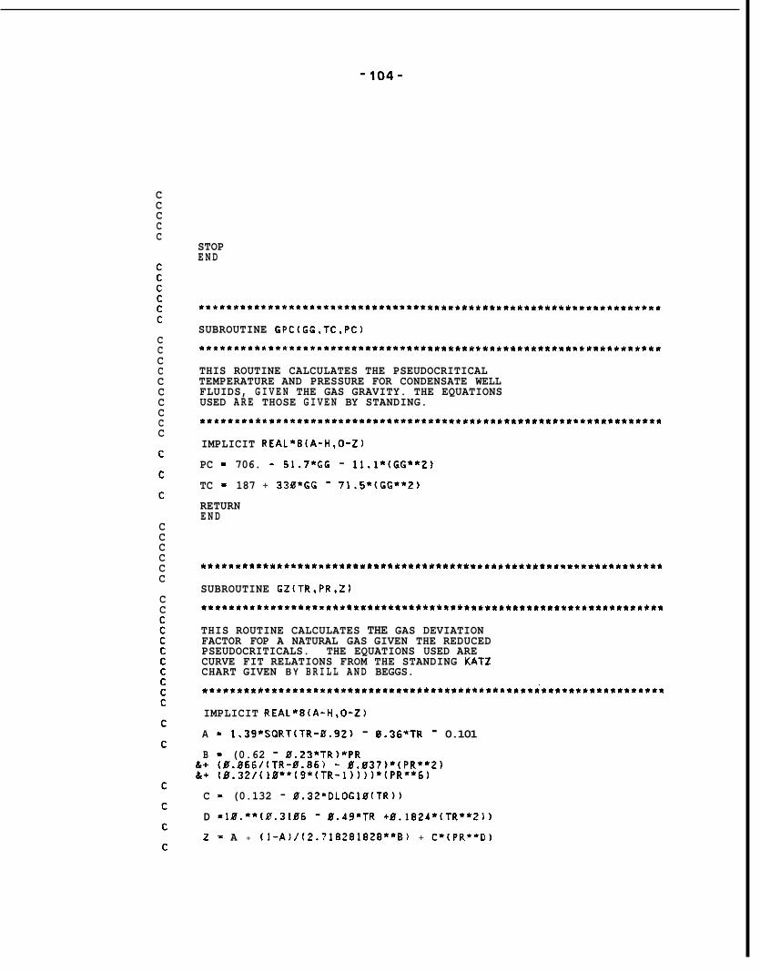
- 104-

C C C C C

STOP E N D

C C C C C C C C C C

C C C C C C

C C

SUBROUTINE GPC(GG.TC.PC) . . . . . . . . . . . . . . . . . . . . . . . . . . . . . . . . . . . . . . . . . . . . . . . . . . . . . . . . . . . . . . . . . . . . . . . . .

THIS ROUTINE CALCULATES THE PSEUDOCRITICAL TEMPERATURE AND PRESSURE FOR CONDENSATE WELL FLUIDS, G I V E N THE GAS GRAVITY. THE EQUATIONS USED A R E THOSE G I V E N BY STANDING. I * * * * * * * * t W * * * * * * * * * * * * * * * * * * * C * * L e * * * * * * * * * * * * * * * * * * * * * * * * * * * * * R * * * * * * *

IMPLICIT REAL*E(A-H,O-Z)

PC = 706. - 51.7*GG - 11.1*(66**2) TC 187 + 330*GG - 71.5*(GG**2) RETURN E N D

* * * * * * * * * * * * * * * * * * * * * * * m n * * * * * * * * * * * * * * * * * * * * * * * * * * * * * * * * * * * * * * * * * *

SUBROUTINE GZ(TR.PR.2) *****************n*************************************************

THIS ROUTINE CALCULATES THE GAS DEVIATION FACTOR FOP A NATURAL GAS GIVEN THE REDUCED PSEUDOCRITICALS. THE EQUATIONS USED ARE CURVE FIT RELATIONS FROM THE STANDING KAT2 CHART GIVEN B Y B R I L L A N D BEGGS. **t***********************.*********.*********R****~******************

IMPLICIT REAL*E(A-H.O-Z)

A = 1.39*SQRT(TR-ff.92) - 9.36*TR - 0.101 B = (0.62 - 0.23*TR)*PR

&+ (0.066/(TR-0.86) - 0.037)*(PR**2) &+ (0.32/(18**(9*(TR-l))))*(PR**6)

C = (0.132 - 0.3ZRDLOG10(TR)) D =10.**(0.3106 - 0.49*TR +0.1824*(TR**2))

2 = A + (i-A)/(2.718281828**B) + C*(PR**D)

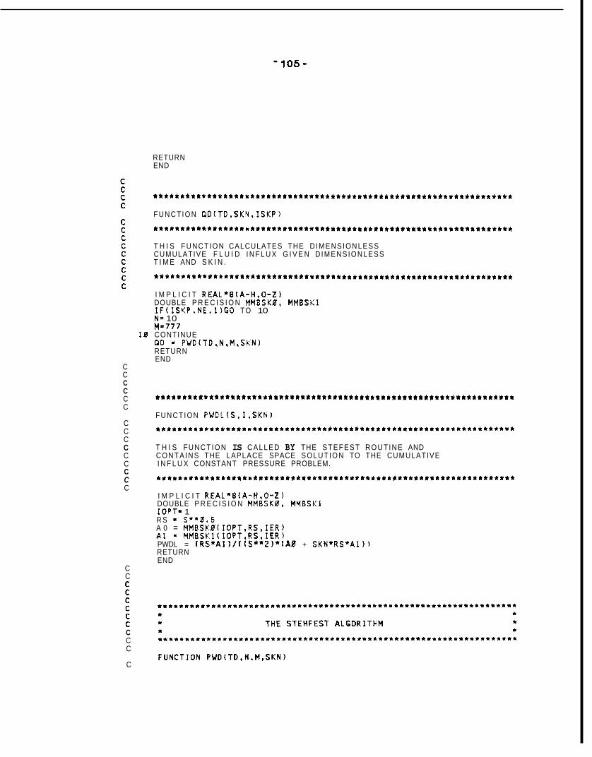
- 105-

RETURN END

C C C C C C

C C C C C C C C C

. . . . . . . . . . . . . . . . . . . . . . . . . . . . . . . . . . . . . . . . . . . . . . . . . . . . . . . . . . . . . . . . . . . . . .

F U N C T I O N Q D ( T D , S K N , I S K P )

*****************r**************.t********************~****************

T H I S F U N C T I O N CALCULATES THE D I M E N S I O N L E S S CUMULATIVE F L U I D I N F L U X G I V E N D I M E N S I O N L E S S T I M E AND S K I N .

. . . . . . . . . . . . . . . . . . . . . . . . . . . . . . . . . . . . . . . . . . . . . . . . . . . . . . . . . . . . . . . . . . . . . .

I M P L I C I T R E A L * 8 ( A - H , O - Z ) DOUBLE P R E C I S I O N MMBSK0, MMBSKI I F ( I S K P . N E . 1 ) G O TO 10 N= 10

10 CONTINUE M=777

OD - PWD(TD.N.M.SKN) RETURN END

. . .

*****************r************.**.**************************************

F U N C T I O N P W D L ( S , I . S K N )

T H I S F U N C T I O N IS C A L L E D BY THE S T E F E S T R O U T I N E AND C O N T A I N S THE LAPLACE SPACE S O L U T I O N TO THE CUMULATIVE I N F L U X CONSTANT PRESSURE PROBLEM.

DOUBLE P R E C I S I O N MMBSK0, MMBSKI I M P L I C I T R E A L * B ( A - H , O - Z )

I O P T = 1 R S - S * * 0 . 5 A 0 = M M B S K B ( I O P T , R S , I E R ) A 1 = M M B S K l ( I O P T , R S , I E R ) PWDL = ( R S * A l ) / ( ( S * * ? ) * ( A B + S K N * R S * A l ) ) RETURN END

C C

C C C

C

- 106-

C T H I S F U N T I O N COMPUTES NUMERICALLY THE L A P L A C E TRNSFORM C INVERSE OF F C S ) . THE R O U T I N E WAS WRITTEN BY DR. A. SAGEEV C OF STANFORD U N I V E R S I T Y . C C C

* * * * * * * * * * * * * * * * * * * * * * * * * * * * * * * * . * * . * * * * * * * ~ * * * * * * * * * * * * * * * w * * * * * * * * * *

I M P L I C I T R E A L * 8 fA -H ,O-Z ) D I M E N S I O N G ( 5 0 ) , V ! 5 0 ) , H ( 2 5 )

C C*****NOW I F THE ARRAY V ( I ) WAS COMPUTED BEFORE T h E PROGRAM

C F ( S ) . C

C GOES D I R E C T L Y TO THE END O f THE SUBROUTINE TO CALCULATE

I F (N.EQ.M) GO TO 1 7 M=N D L O G T W = 0 . 6 9 3 1 4 7 1 8 0 5 5 9 9 NH=N/Z

C C * * * * * T H E F A C T O R I A L S OF 1 TO N ARE CALCULATED I N T O ARRAY G . C

G ( 1 ) = l DO 1 I - 2 , N G ( I ) = G ( I - l ) * I

1 C

CONTINUE

C*****TERMS W I T H K ONLY ARE CALCULATED I N T O ARRAY H. C -

H ( l ) = Z . / G ( N H - I ) DO 6 I - 2 , N H F I = I I F l I - N H ) 4 , 5 , 6

GO TO 6 4 H(I)~FI**NH*G(2*I)/~G~NH-I)*G(I)*G(I-l)~

5 6 CONT 1 NUE

H(I)~FI**NH*G(2*I)/(G(I)*G(I-1))

C C * * * * * T H E TERMS ( - l ) * * N H + l ARE CALCULATED. C F I R S T THE TERM FOR 111 C

C

C C * * * * * T H E R E S T OF THE SN'S ARE CALCULATED I N THE M A I N R O U T I N E

S N = 2 * ( N H - N H / Z * 2 ) - 1

C C C*** * *THE ARRAY V ( 1 ) IS CALCULATED. C

C DO 7 I = l , N

C * * * * * F I R S T S E T V(I)=0 C

C C * * * * * T H E L I M I T S FOR K ARE E S T A B L I S H E D . C C

THE LOWER L I M I T IS K l r I N T E G ( ( I + 1 / 2 ) )

C Kl=(I+l)/Z

C * * * * * T H E UPPER L I M I T IS K Z = M I N ( I , N / 2 ) C

V ( I ) = 0 .

K 2 = I I F ( K 2 - N H ) 8 , 8 , 9

- 107 -

9 KL=NH C C*****THE SUMMATION TERM I N C 8 DO 10 K=Kl ,K2

11 V(I)IJ(I)+H(K)/(G(I-K

IF (2*K-I) 12.13.12 12 IF ( I - K ) 11.14.11

GO TO 10 13 V(I)=V(I)+H(K)/G(I-K)

GO TO 10 1 4 V(I)=V(J)+H(K)/G(Z*K- 10 CONTINUE c

V f I ) IS CALCULATED.

)*G(L*K-I))

I )

c. C*****THE V 1 I ) ARRAY IS FINALLY CALCULATED BY WEIGHTING C ACCORDING TO SN. C

C C*****THE TERM S N CHANGES ITS SIGN EACH ITERATION. C

7 SN=-SN CONTINUE

C C*****THE NUMERICAL APPROXIMATION IS CALCULATED.

V(I)=SN*V(I)

c 17 PWD=0.

A=DLOGTW/TD DO 15 1el.N ARG=A* I PUD=PWD+V(I)*PWDL(ARG,I,SKN)

PWD=PWD*A 15 CONTINUE

18 RETURN EN D

APPENDIX B

BASECASE NUMERICAL VALUES

- 109 -

I N P U T DATA A S FOLLOWS:

CUTPUT F I L E NAME =

CHAMBE3 DIAMETER = TOTAL CHAMBER LENGTH FROM PERFORATIONS - I N I T I A L F L U S D COLUMN LENGTH = I N I T I A L CHAMBER PRESSURE * CHAMBER GAS G R A V I T Y =

I N I T I A L R E S E R V O I T PRESSURE = CHAMBER GAS TEMPERATl iRE = PRODUCED F L U I D S P E C I F I C G R A V i T Y =

RESERVDIR P O R O S I T Y = PRODUCED F L U I D V I S C O S I T Y =

RESERVOIR P E R M E A B I L I T Y = S K I N = L E L L DIAMETER - FORMATION TOTAL C O M P R E S S I B I L i T Y = FORMATION T H I C K N E S S =

TOTAL T E S T T I M E = T I M E IVCREMENT = NUMBER OF T I M E STEPS = NUMBER OF DATA P O I N T S =

b a s a c a s a

0 . 2 8 3 ( F E E T ) 1 0 0 0 . b P ( F E E T )

100 .UP ( F E E T ) 4 4 . 7 0 ( P S I A )

0.65UG ( A I R = 1 . 0 )

5 0 1 4 . 7 0 ( P S I A ) 6 3 5 . 8 P t R ) 0 . 9 0 5 2

1 . 2 5 P ( C P ) 0 . 2 7 U g 1 0 0 . U 6 ( M D )

0 . 8 3 3 3 ( F E E T )

2 5 . 0 6 ( F E E T )

100.00bEf (SECONDS) 0.01086 (SECONDS)

0 .

0 . 1 0 0 0 e - 0 4 ( 1 / P S I )

1000d 1 0 M

(SECONDS) T I M E

b. 1 .El0200 2 . 0 0 a 0 0 3 . 0 0 8 0 0 4 . 0 0 3 0 0 5 . 0 0 8 0 0

7 . 0 0 3 0 0 6 . 0 0 a 0 8

8 . 0 0 3 0 0 9 . 0 0 2 0 0

18.08800 1 1.00a00 1 2 . 0 0 8 0 0 1 3 . 0 0 a 0 0 1 4 . 0 0 8 0 0 1 5 . 0 0 3 0 0 16 .0BB00 1 7 . 0 0 a 0 0 1 8 . 0 0 8 0 0 1 9 . 0 0 a 0 0 2J3.00.800 2 1 . 0 0 8 0 0 2 2 . 0 0 a 0 0 2 3 . 0 0 3 0 0 2 4 . 8 0 2 0 0

( P S I A ) P w f

8 3 . 8 7 1 2 7 . 1 1 1 5 6 . 7 8 1 8 4 . 0 5 2 1 0 . 2 5 2 3 6 . 0 2 2 6 1 . 7 9 2 8 7 . 9 4 3 1 4 . 8 7 3 4 3 . 0 9 3 7 3 . 2 4 4 0 6 . 2 7 4 4 3 . 6 1 4 8 7 . 6 2 5 4 2 . 4 3 6 1 5 . 9 6 7 2 5 . 1 6 91 1 . 5 9

1 2 8 7 . 6 8 2 0 5 5 . 6 8 2 8 7 9 . 1 4 3 3 1 2 . 8 7 3 5 5 7 . 0 9 3 7 2 2 . 2 3 3 8 4 5 . 5 6

F L D PRD [ B B L S )

0. 0 . 5 5 9 5 0 . 9 3 3 5 1 . 2 6 8 4 1 . 5 8 0 8 1 .E776 2 . 1 6 2 5 2 . 4 3 7 8 2 . 7 0 4 8 2 . 9 6 4 6 3 . 2 1 7 9 3 . 4 6 5 1 3 . 7 0 6 3 3 . 9 4 1 6 4 . 1 7 0 5 4 . 3 9 2 1 4 . 6 0 4 1 4 . 8 0 1 5 4 . 9 7 2 8 5 . 0 8 6 6 5 . 1 2 8 9 5 . 1 4 0 5 5 . 1 4 5 4 5 . 1 4 8 2 5 . 1 5 0 8

X ( F E E T )

100.80 1 9 6 . 6 8 2 6 1 . 2 9 3 1 9 . 1 5 3 7 3 . 1 2 4 2 4 . 4 1 4 7 3 . 6 4 5 2 1 . 1 9 5 6 7 . 3 3 6 1 2 . 2 2 6 5 5 . 9 8 6 9 8 . 6 8 7 4 0 . 3 6 7 8 1 . 0 2 8 2 0 . 5 7 8 5 8 . 8 5 8 9 5 . 4 8 9 2 9 . 5 9 9 5 9 . 0 5 9 7 8 . 8 5 9 8 6 . 1 6 9 8 8 . 1 7 9 8 9 . 0 1 9 8 9 . 4 9 9 8 9 . 8 0

( P S I A ) P c h

4 4 . 7 0 5 0 . 0 5 5 4 . 4 1 5 9 . 0 1 6 4 . 0 7 6 9 . 7 5 7 6 . 2 3 8 3 . 7 5 9 2 . 6 1

1 0 3 . 2 4 1 1 6 . 2 5 1 3 2 . 5 5 1 5 3 . 5 6 1 8 1 . 6 4 2 2 0 . 9 6 2 7 9 . 4 9 3 7 4 . 3 4 5 4 7 . 4 8 9 1 1 . 9 5

1 6 7 2 . 1 9 2 4 9 2 . 7 9 2 9 2 5 . 7 3 3 1 6 9 . 6 3 3 3 3 4 . 5 8 3 4 5 7 . 7 9

z

0 . 9 9 6 4 0 . 9 9 5 9 0 . 9 9 5 6 0 . 9 9 5 2 0 . 9 9 4 8 0 . 9 9 4 3 0 . 9 9 3 8 0 . 9 9 3 2 0 . 9 9 2 5 0 . 9 9 1 6 0 . 9 9 0 6 0 . 9 8 9 2 0 . 9 8 7 5 0 . 9 8 5 2 0 . 9 8 2 0 0 . 9 7 7 1 0 . 9 6 9 2 0 . 9 5 4 6 0 . 9 2 4 9 0 . 8 7 6 0 0 . 8 5 4 5 0 . 8 5 7 5 0 . 8 6 3 2 0 , 8 6 8 5 0 . 8 7 3 2

I F L A G

0 0 0 0 0 0

0 0

0 0 0 0 0 0 0 0 0 0 0 0 0 0 0 0 0

- 1 1 0 -

25.00000 26.00300 27.00300

29.00300 38.00300 3 1.00800 32.00300 3 3.00300 34.00800 35.00a00 3 6.00800 37.00 300 38.00 a00 39.00300 48 * 00 a00 4 1 .00.a00 4 2.00a00 4 3.00300 4 4.00a00 45.00800 4 6.00800 4 7.00300 48 -00200 4 9.00.a00 511.00300 5 1.00300 52.00200 5 3.00800 5 4 .00300 5 5.00200 5 6 .00.a00 5 7 .00a00

5 9.00.800 68.00 a00 61.00100 6 2 .00300 63.001E0 6 4.00.a00

6 6.00.808 67 .00300 6 8.00200 6 9 .00800 70.00800 7 1.00a00 7 2.00B00 7 3 .002B0

7 5 .00200 76.00100 77.00.100 78.00Zf00 79.00a00 811 .OO a00 8 1 .OO 300 82.00300 83.00100 8 4 .00.100 85.00300 8 6 .00300 87.00300 88.00300

28.00 a00

58 .ma00

65 .80300

74 . ~ 0 1 ~ m

3343.06 4023 .OO 4090.22 4147.84 4197.95 4242.06 4281.25 4316.37 4348.05 4376.81 4403.05 4427.10 4449.25 4469.72 4488.69 4506.34 4522.80 4538.20 4552.63 4566.19 4578.95 4590.99 4602.36 4613.13 4623.33 4633.02 4642.23 4651 .OO 4659.36 4667.34 4674.96 4682.25 4689.22 4695.91 4702.32 4708.48 4714.40 4720.08 4725.56 4730.83 4735.91 4740.82 4745.55 4750.11 4754.53 4758.80 4762.93 4766.92 4770.79 4774.54 4778.18

4785.13 4781.71

4791.68 4788.45

4794.81 4797.86 4800.83 4803.71 4806.52 4809.25 481 1.91 4814.51 4817.03

5.1514 5.1524 5.1532 5.1539 5.1544 5.1549 5.1553 5.1557 5.1568 5.1563 5.1566 5.1568 5.157U 5.1572 5.1574 5.1575 5.1577 5.1578 5.1579 5.1581 5.1582 5.1583 5.1584 5.1585 5.1585 5.1586 5.1587 5.1588 5.1588 5.1589 5.1598 5.1598 5.159i 5.1591 5.1592 5.1592 5.1593 5.1593 5.1594 5.1594 5.1594 5.1595 5.1595 5.1596 5.1596 5.1596 5.1597 5.1597 5.1597 5.1597 5.1596 5.1598 5.1598

5.1599 5.1598

5.1599 5.1599 5.1599 5.1608 5.1608 5.1608 5.1608 5.160fi 5.160i

990.04 990.22 990.36 990.47 990.57 990.65 990.73 990.79 990.84 990.89 990.94 990.98 991 .O1 991.05 991.08 991.10 991.13 991.15 991.17 991.19 991.21 991.23 991.25 991.26 991.28 991.29 991.31 991.32 991.33 991.34 991.35 991.36 991.37 991.38 991.39 991.40 991.41 991.41 991.42 991.43 991.43 991.44 991.45 991.45 991.46 991.47 991.47 991.48 991.48 991.49 991.49 991.50 991.50 991.50 991.51 991.51 991.52 991.52 991.52 991.53 991.53 991.53 991.54 991.54

3555.20 3635.06 3702.23 3759.80 3809.. 88 3853.95 3893.11 3928.21 3959.87 3988.60 4014.83 4038.87 4061 .I0 4081.45 4100.42 41 18.06 4134.51 4149.90 4164.32 4177.87 4190.62 4202.65 4214.02 4224.78 4234.98 4244.66 4253.87 4262.63 4270.99 4278.96 4286.58 4293.86 4300.83 4307.52 4313.93 4320.08 4325.99 4331.68 4337.15 4342.42 4347.50 4352.48 4357.13 4361.69 4366.10 4370.37 4374.50 4378.49 4382.36 4386.11 4389.74 4393.27 4396.69 4400.01 4403.24 44S6.37 4409.42 4412.38 4415.26 4418.07 4420.80 4423.46 4426.05 4428.58

0.0774 0.8810 0 . 8843 0.8872 0.8898 0.8921 0.8943 0.8963 0.8981 0.8997 0.901 3 0.9027 0.9040 0.9052 0.9064 0.9075 0.9085 0.9095 0.9104 0.9112 0.9120 0.9128 0.9135 0.9142 0.9149 0.9155 0.9161 0.9167 0.9172 0.9178 0.9183 0.9187 0.9192 0.9196 0.9201 0.9205 0.9209 0.9213 0.9216 0.9220 0.9223 0.9226 0.9230 0.9233 0.9236 0.9239 0.9241 0.9244 0.9247 0.9249 0.9252 0.9254 0.9257 0.9259 0.9261 0.9263 0.9265 0.9267 0.9269 0.9271 0.9273 0.9275 0.9277 0,9278

0 0 0 0 0 0 0 0 0 0 0 0 0 0 0 0 0 0 0 0 0 0 0 0 0 0 0 0 0 0 0 0 0 0 0 0 0 0 0 0 0 B 0 0 0 0 0 0 0 0 0 0 0 0 0 0 0 0 0 0 0 0 0 0

1

- 111 -

89.00600 91T. 00800 9 1.00808

93.00108 94.00800 95.10300 9 6.00300 9 7.00a00 98.00800 99.00108 100.00 300

92 .ma00

4819.50 5.1601 4821.90 5.1601 4824.24 5.1601 4826.53 5.1601 4828.76 5.1601 4830.94 5.1602 4833.07 5.1602 4835.15 5.168'2 4837.19 5.1602 4839.18 5.1602 4841.12 5.160'2 4843.02 5.1603

991.54 4431.04 991.55 4433.44 991.55 4435.78 991.55 4438.07 991.56 4440.38 991.56 4442.48 991.56 4444.61 991.56 4446.69 991.57 4448.72 991.57 4450.71 991.57 4452.65 991.57 4454.55

0.9280 0.9282 0.9283 0.9285 0.9287 0.9288 0.9289 0.9291 0.9292 0.9294 1. 9295 0.9296

0 0 0 0 0 0 0 0 0 0 0 0

Closed Chamber Well Test Analysis by Superposition of the … · test as often does a conventional...

Documents

Transcript of Closed Chamber Well Test Analysis by Superposition of the … · test as often does a conventional...