Clopper-Pearson Confidence Interval in SAS Using Proc · PDF fileAnik Chatterjee Novartis,...
26
Anik Chatterjee Novartis, Hyderabad, India Clopper-Pearson Confidence Interval in SAS Using Proc Freq Disclaimer: The views expressed within this paper/presentation are entirely that of the author and do not necessarily reflect the views of Novartis AG.
Transcript of Clopper-Pearson Confidence Interval in SAS Using Proc · PDF fileAnik Chatterjee Novartis,...

Anik Chatterjee
Novartis, Hyderabad, India
Clopper-Pearson Confidence Interval in SAS Using Proc Freq
Disclaimer: The views expressed within this paper/presentation are entirely that of the author and do not necessarily reflect the views of Novartis AG.
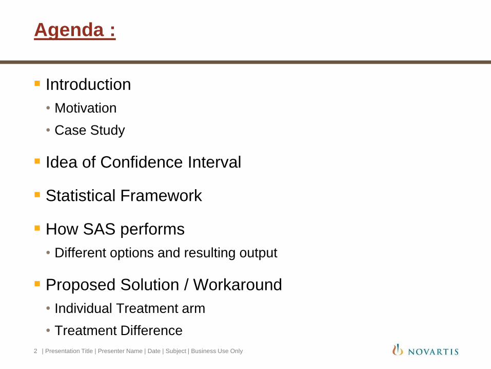
Agenda :
| Presentation Title | Presenter Name | Date | Subject | Business Use Only 2
Introduction
• Motivation
• Case Study
Idea of Confidence Interval
Statistical Framework
How SAS performs
• Different options and resulting output
Proposed Solution / Workaround
• Individual Treatment arm
• Treatment Difference
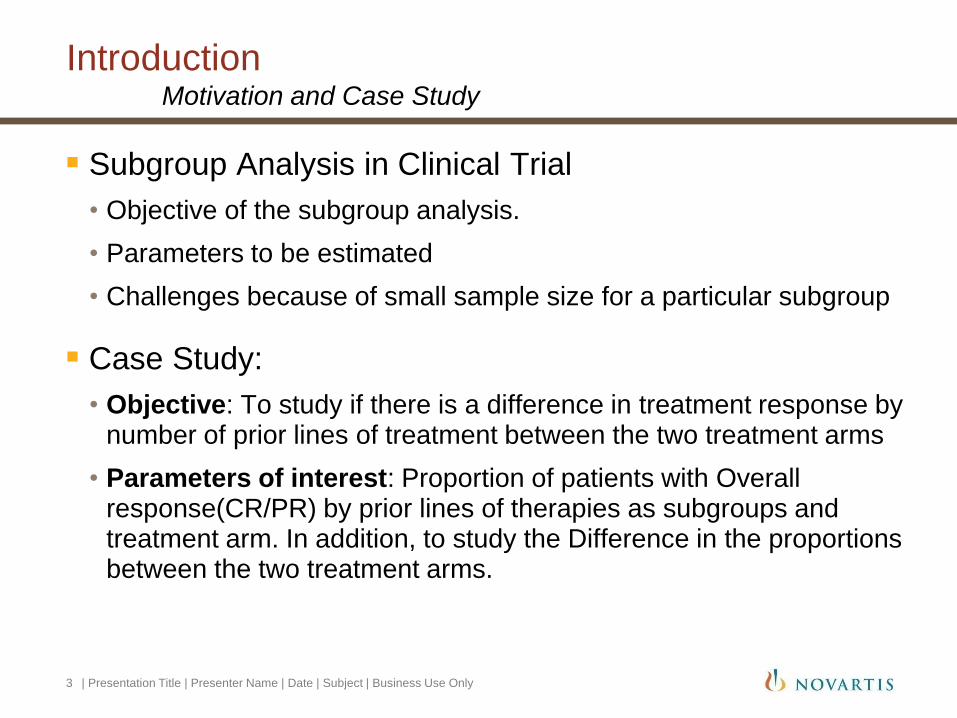
Introduction
| Presentation Title | Presenter Name | Date | Subject | Business Use Only 3
Motivation and Case Study
Subgroup Analysis in Clinical Trial
• Objective of the subgroup analysis.
• Parameters to be estimated
• Challenges because of small sample size for a particular subgroup
Case Study:
• Objective: To study if there is a difference in treatment response by number of prior lines of treatment between the two treatment arms
• Parameters of interest: Proportion of patients with Overall response(CR/PR) by prior lines of therapies as subgroups and treatment arm. In addition, to study the Difference in the proportions between the two treatment arms.
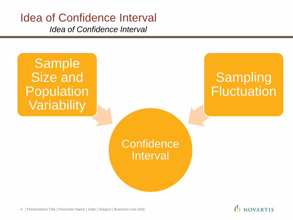
Idea of Confidence Interval
| Presentation Title | Presenter Name | Date | Subject | Business Use Only 4
Idea of Confidence Interval
Confidence Interval
Sample Size and
Population Variability
Sampling Fluctuation
Idea of Confidence Interval
| Presentation Title | Presenter Name | Date | Subject | Business Use Only 5
Sample and Population
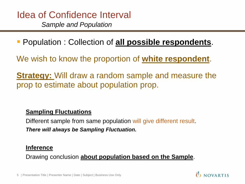
Population : Collection of all possible respondents.
We wish to know the proportion of white respondent.
Strategy: Will draw a random sample and measure the prop to estimate about population prop.
Sampling Fluctuations
Different sample from same population will give different result.
There will always be Sampling Fluctuation.
Inference
Drawing conclusion about population based on the Sample.
Idea of Confidence Interval
| Presentation Title | Presenter Name | Date | Subject | Business Use Only 6
Different Sampling methods
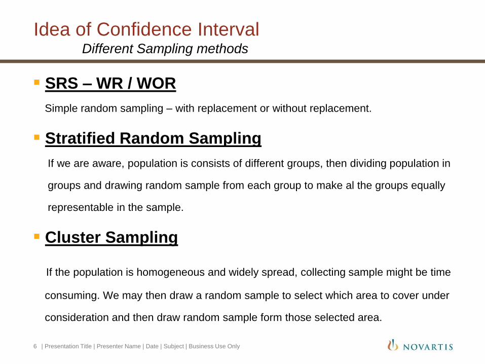
SRS – WR / WOR
Simple random sampling – with replacement or without replacement.
Stratified Random Sampling
If we are aware, population is consists of different groups, then dividing population in
groups and drawing random sample from each group to make al the groups equally
representable in the sample.
Cluster Sampling
If the population is homogeneous and widely spread, collecting sample might be time
consuming. We may then draw a random sample to select which area to cover under
consideration and then draw random sample form those selected area.
Idea of Confidence Interval
| Presentation Title | Presenter Name | Date | Subject | Business Use Only 7
Sampling Fluctuations and Inference
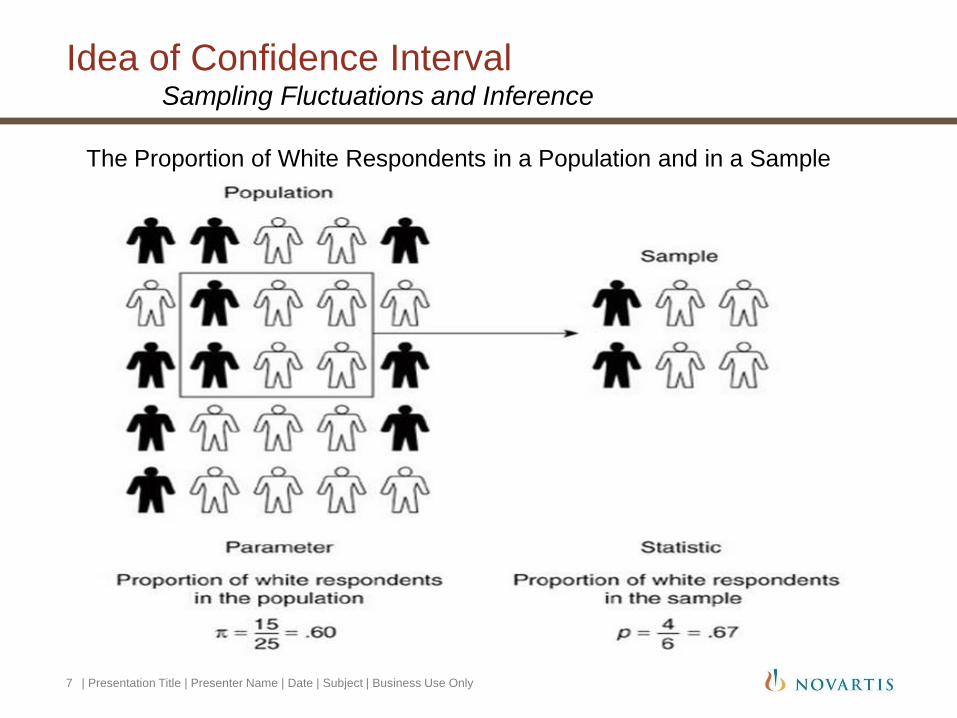
The Proportion of White Respondents in a Population and in a Sample

Idea of Confidence Interval
| Presentation Title | Presenter Name | Date | Subject | Business Use Only 8
Variation within the population
Less/More variation(P) => Less/More variation(S)
Idea of Confidence Interval
| Presentation Title | Presenter Name | Date | Subject | Business Use Only 9
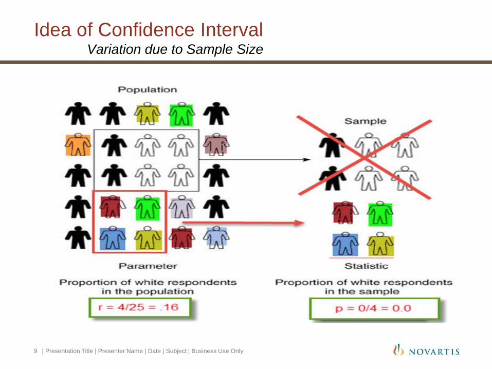
Variation due to Sample Size
Idea of Confidence Interval
| Presentation Title | Presenter Name | Date | Subject | Business Use Only 10
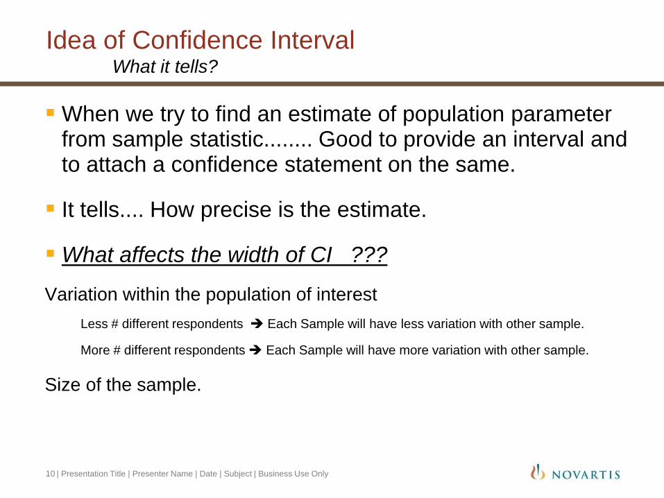
What it tells?
When we try to find an estimate of population parameter from sample statistic........ Good to provide an interval and to attach a confidence statement on the same.
It tells.... How precise is the estimate.
What affects the width of CI ???
Variation within the population of interest
Less # different respondents Each Sample will have less variation with other sample.
More # different respondents Each Sample will have more variation with other sample.
Size of the sample.
Idea of Confidence Interval
| Presentation Title | Presenter Name | Date | Subject | Business Use Only 11
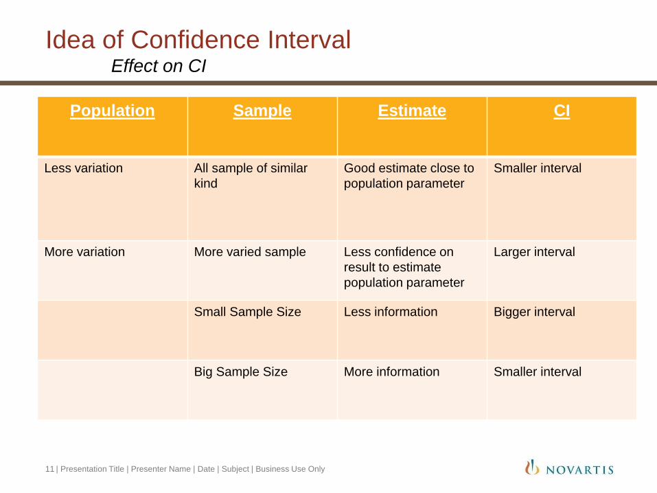
Effect on CI
Population Sample Estimate CI
Less variation All sample of similar
kind
Good estimate close to
population parameter
Smaller interval
More variation More varied sample Less confidence on
result to estimate
population parameter
Larger interval
Small Sample Size Less information Bigger interval
Big Sample Size More information Smaller interval
Idea of Confidence Interval
| Presentation Title | Presenter Name | Date | Subject | Business Use Only 12
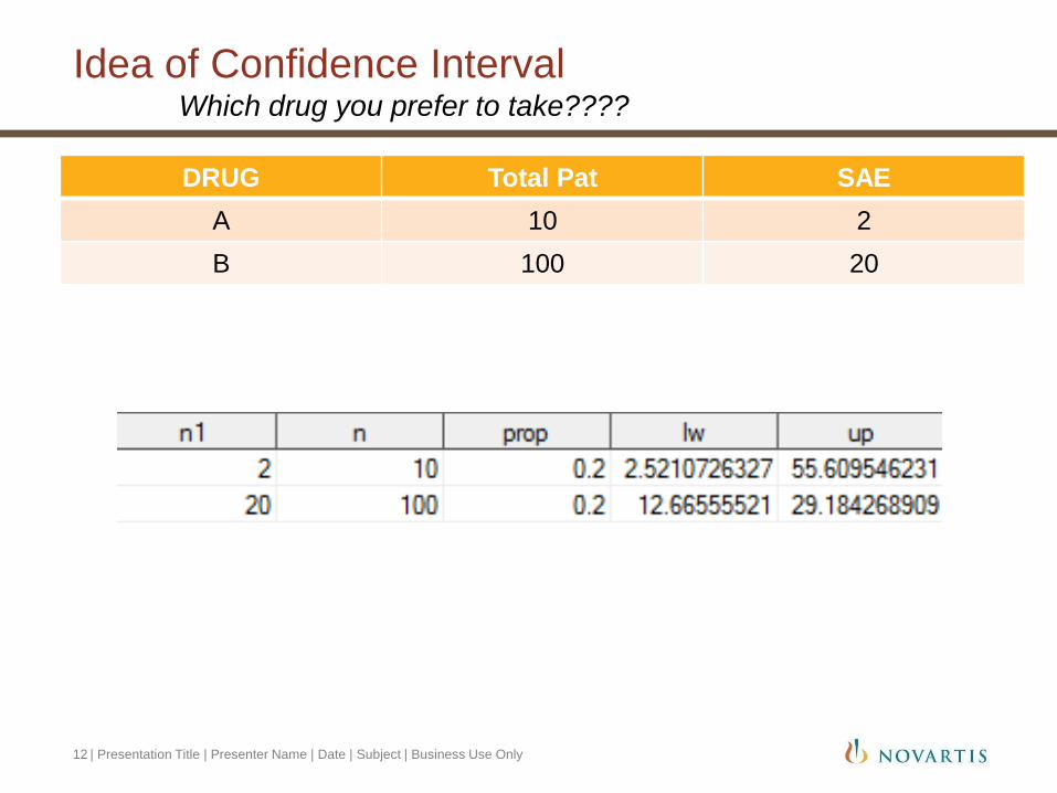
Which drug you prefer to take????
DRUG Total Pat SAE
A 10 2
B 100 20
Statistical Framework
| Presentation Title | Presenter Name | Date | Subject | Business Use Only 13
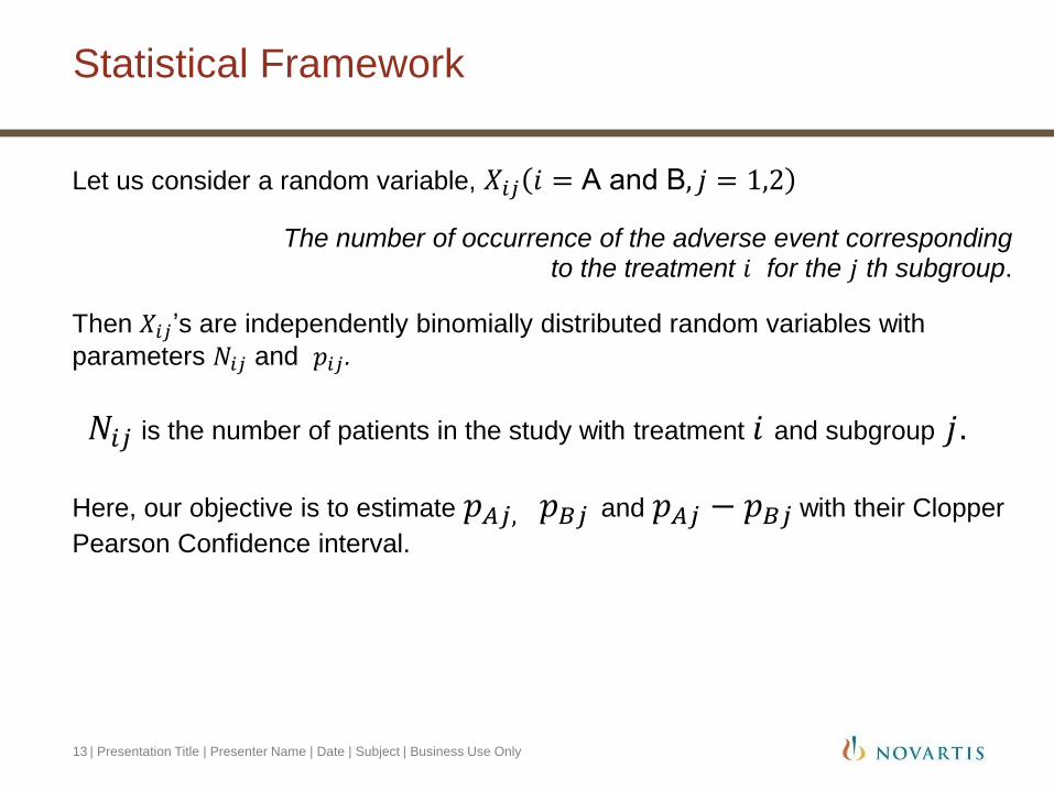
Let us consider a random variable, 𝑋𝑖𝑗 𝑖 = A and B, 𝑗 = 1,2
The number of occurrence of the adverse event corresponding to the treatment 𝑖 for the 𝑗 th subgroup.
Then 𝑋𝑖𝑗’s are independently binomially distributed random variables with
parameters 𝑁𝑖𝑗 and 𝑝𝑖𝑗.
𝑁𝑖𝑗 is the number of patients in the study with treatment 𝑖 and subgroup 𝑗.
Here, our objective is to estimate 𝑝𝐴𝑗, 𝑝𝐵𝑗 and 𝑝𝐴𝑗 − 𝑝𝐵𝑗 with their Clopper
Pearson Confidence interval.
Statistical Framework
| Presentation Title | Presenter Name | Date | Subject | Business Use Only 14
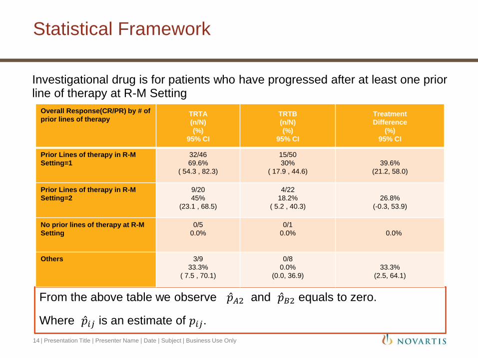
Investigational drug is for patients who have progressed after at least one prior line of therapy at R-M Setting
From the above table we observe 𝑝 𝐴2 and 𝑝 𝐵2 equals to zero.
Where 𝑝 𝑖𝑗 is an estimate of 𝑝𝑖𝑗.
Overall Response(CR/PR) by # of
prior lines of therapy TRTA
(n/N)
(%)
95% CI
TRTB
(n/N)
(%)
95% CI
Treatment
Difference
(%)
95% CI
Prior Lines of therapy in R-M
Setting=1
32/46
69.6%
( 54.3 , 82.3)
15/50
30%
( 17.9 , 44.6)
39.6%
(21.2, 58.0)
Prior Lines of therapy in R-M
Setting=2
9/20
45%
(23.1 , 68.5)
4/22
18.2%
( 5.2 , 40.3)
26.8%
(-0.3, 53.9)
No prior lines of therapy at R-M
Setting
0/5
0.0%
0/1
0.0%
0.0%
Others 3/9
33.3%
( 7.5 , 70.1)
0/8
0.0%
(0.0, 36.9)
33.3%
(2.5, 64.1)

Statistical Framework
| Presentation Title | Presenter Name | Date | Subject | Business Use Only 15
The Clopper- Pearson method is capable of finding the confidence interval of 𝑝 𝑖𝑗 when its estimate is zero.
Please see the screenshot below Clopper Pearson(1934). The green circle shows the CI for p when estimate of p = 0 for n=10.
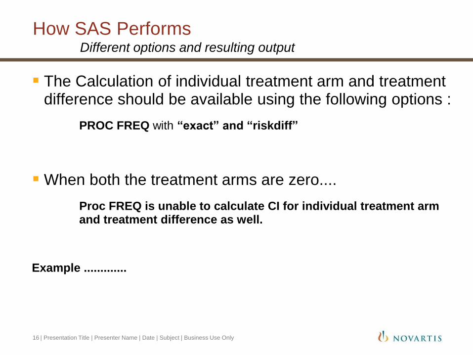
How SAS Performs
| Presentation Title | Presenter Name | Date | Subject | Business Use Only 16
Different options and resulting output
The Calculation of individual treatment arm and treatment difference should be available using the following options :
PROC FREQ with “exact” and “riskdiff”
When both the treatment arms are zero....
Proc FREQ is unable to calculate CI for individual treatment arm and treatment difference as well.
Example .............
| Presentation Title | Presenter Name | Date | Subject | Business Use Only 17
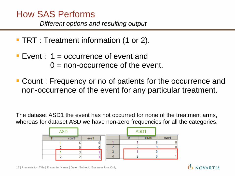
Different options and resulting output
TRT : Treatment information (1 or 2).
Event : 1 = occurrence of event and 0 = non-occurrence of the event.
Count : Frequency or no of patients for the occurrence and non-occurrence of the event for any particular treatment.
The dataset ASD1 the event has not occurred for none of the treatment arms, whereas for dataset ASD we have non-zero frequencies for all the categories.
How SAS Performs
| Presentation Title | Presenter Name | Date | Subject | Business Use Only 18
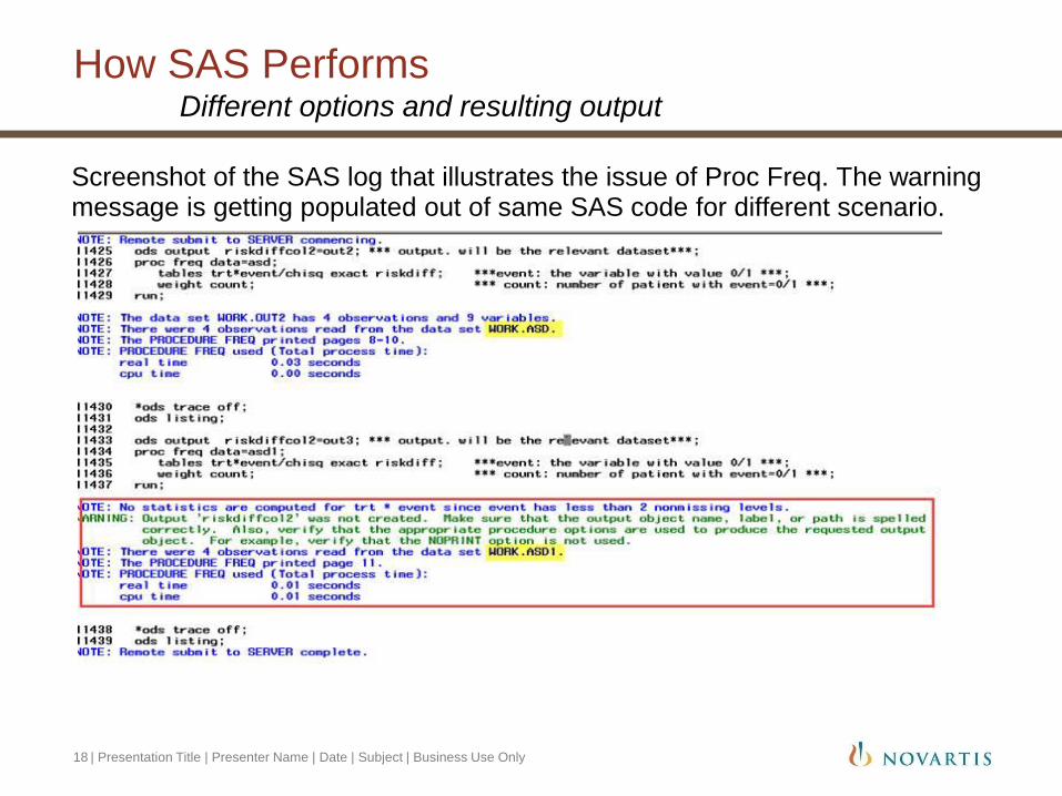
Different options and resulting output
Screenshot of the SAS log that illustrates the issue of Proc Freq. The warning message is getting populated out of same SAS code for different scenario.
How SAS Performs
| Presentation Title | Presenter Name | Date | Subject | Business Use Only 19
Different options and resulting output
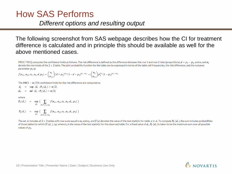
The following screenshot from SAS webpage describes how the CI for treatment difference is calculated and in principle this should be available as well for the above mentioned cases.
How SAS Performs
| Presentation Title | Presenter Name | Date | Subject | Business Use Only 20
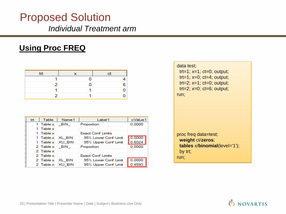
Individual Treatment arm
Using Proc FREQ
Proposed Solution
data test;
trt=1; x=1; ct=0; output;
trt=1; x=0; ct=4; output;
trt=2; x=1; ct=0; output;
trt=2; x=0; ct=6; output;
run;
proc freq data=test;
weight ct/zeros;
tables x/binomial(level='1');
by trt;
run;
| Presentation Title | Presenter Name | Date | Subject | Business Use Only 21
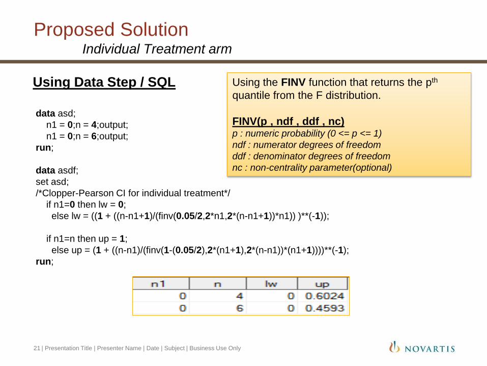
Individual Treatment arm
Using Data Step / SQL
Proposed Solution
data asd;
n1 = 0;n = 4;output;
n1 = 0;n = 6;output;
run;
data asdf;
set asd;
/*Clopper-Pearson CI for individual treatment*/
if n1=0 then lw = 0;
else lw = ((1 + ((n-n1+1)/(finv(0.05/2,2*n1,2*(n-n1+1))*n1)) )**(-1));
if n1=n then up = 1;
else up = (1 + ((n-n1)/(finv(1-(0.05/2),2*(n1+1),2*(n-n1))*(n1+1))))**(-1);
run;
Using the FINV function that returns the pth
quantile from the F distribution.
FINV(p , ndf , ddf , nc) p : numeric probability (0 <= p <= 1)
ndf : numerator degrees of freedom
ddf : denominator degrees of freedom
nc : non-centrality parameter(optional)
| Presentation Title | Presenter Name | Date | Subject | Business Use Only 22
Treatment Difference
Newcombe Interval
A good confidence interval for the difference of proportions will produce an appropriate distribution of coverage probabilities.
The standard Wald interval that SAS produces with PROC FREQ and RISKDIFF produces a zero-width interval when both proportions in a data set are zero.
The Newcombe interval, based on the two individual Wilson intervals, has excellent coverage probabilities and outperforms nearly all other methods.
It is computationally simple and will never give any aberrations (like negative proportions or zero-width intervals).
Proposed Solution
Proposed Solution
| Presentation Title | Presenter Name | Date | Subject | Business Use Only 23
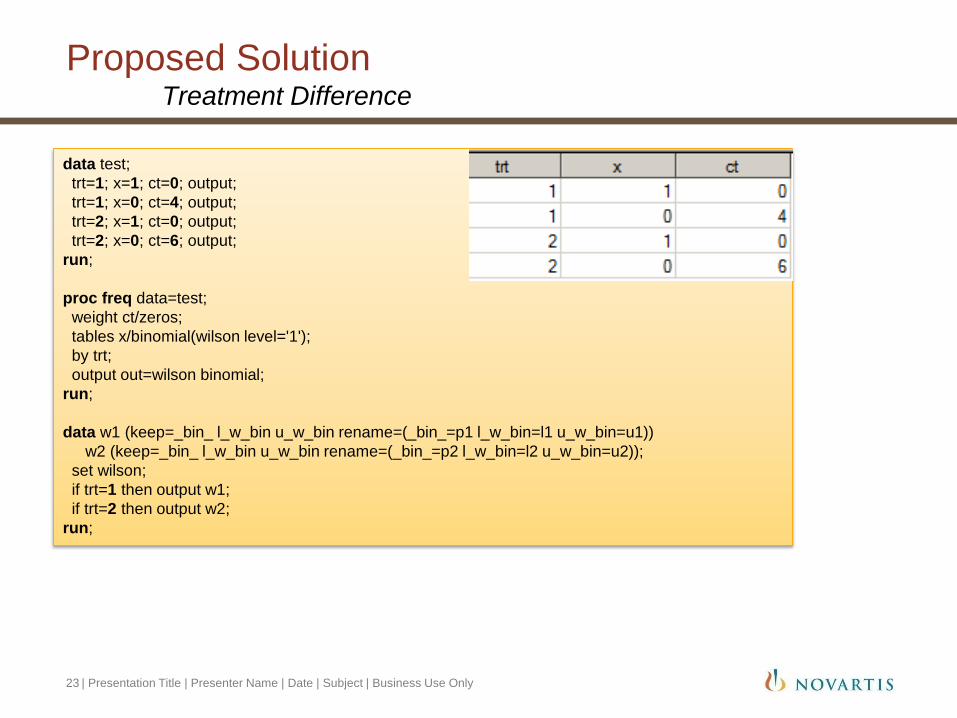
Treatment Difference
data test;
trt=1; x=1; ct=0; output;
trt=1; x=0; ct=4; output;
trt=2; x=1; ct=0; output;
trt=2; x=0; ct=6; output;
run;
proc freq data=test;
weight ct/zeros;
tables x/binomial(wilson level='1');
by trt;
output out=wilson binomial;
run;
data w1 (keep=_bin_ l_w_bin u_w_bin rename=(_bin_=p1 l_w_bin=l1 u_w_bin=u1))
w2 (keep=_bin_ l_w_bin u_w_bin rename=(_bin_=p2 l_w_bin=l2 u_w_bin=u2));
set wilson;
if trt=1 then output w1;
if trt=2 then output w2;
run;
Proposed Solution
| Presentation Title | Presenter Name | Date | Subject | Business Use Only 24
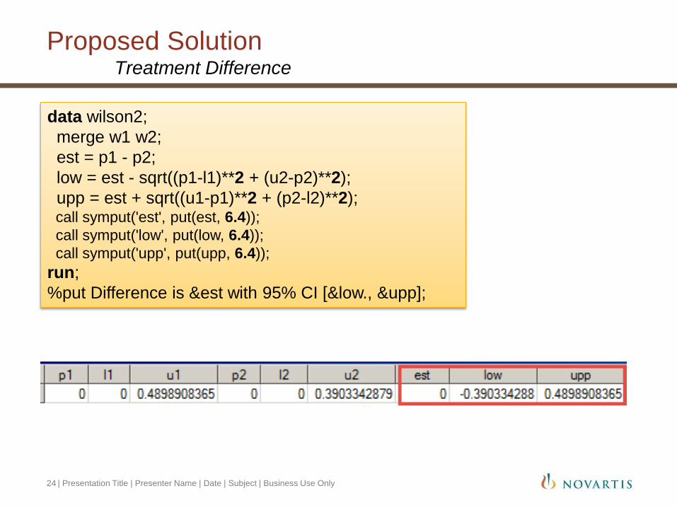
Treatment Difference
data wilson2;
merge w1 w2;
est = p1 - p2;
low = est - sqrt((p1-l1)**2 + (u2-p2)**2);
upp = est + sqrt((u1-p1)**2 + (p2-l2)**2); call symput('est', put(est, 6.4));
call symput('low', put(low, 6.4));
call symput('upp', put(upp, 6.4));
run;
%put Difference is &est with 95% CI [&low., &upp];
References :
| Presentation Title | Presenter Name | Date | Subject | Business Use Only 25
The Use of Confidence or Fiducial Limits Illustrated in the Case of the Binomial
C. J. Clopper; E. S. Pearson
INTERVAL ESTIMATION FOR THE DIFFERENCE BETWEEN INDEPENDENT PROPORTIONS: COMPARISON OF ELEVEN METHODS
ROBERT G. NEWCOMBE

Suggestion and Discussion
| Presentation Title | Presenter Name | Date | Subject | Business Use Only 26
Anik Chatterjee Principal Programmer
Novartis, India
Contact


![Interval Notation: ], not interval notationpgrant.weebly.com/uploads/2/3/2/7/23274454/6.3b_interval_notation.… · •Interval Notation: Uses different brackets to indicate an interval.](https://static.fdocuments.us/doc/165x107/5f8344624904df613146ef90/interval-notation-not-interval-ainterval-notation-uses-different-brackets.jpg)