Clinical PK introduction Lecture 1 2 Clinical Pharmacokinetics in Drug Development • Stage of...
35
Slide 1 Clinical Pharmacokinetics
Transcript of Clinical PK introduction Lecture 1 2 Clinical Pharmacokinetics in Drug Development • Stage of...

Slide 1
Clinical Pharmacokinetics
Slide 2
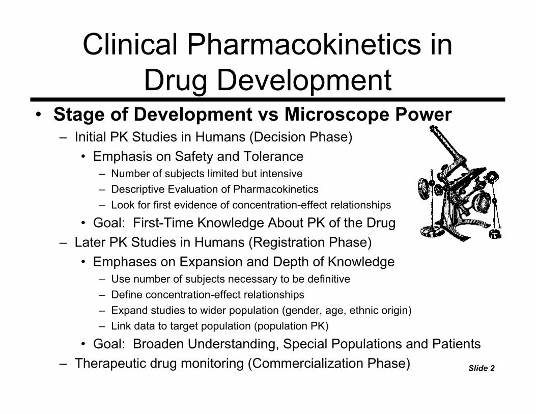
Clinical Pharmacokinetics in Drug Development
• Stage of Development vs Microscope Power– Initial PK Studies in Humans (Decision Phase)
• Emphasis on Safety and Tolerance– Number of subjects limited but intensive– Descriptive Evaluation of Pharmacokinetics– Look for first evidence of concentration-effect relationships
• Goal: First-Time Knowledge About PK of the Drug– Later PK Studies in Humans (Registration Phase)
• Emphases on Expansion and Depth of Knowledge– Use number of subjects necessary to be definitive– Define concentration-effect relationships– Expand studies to wider population (gender, age, ethnic origin)– Link data to target population (population PK)
• Goal: Broaden Understanding, Special Populations and Patients– Therapeutic drug monitoring (Commercialization Phase)

Slide 3
Definitions and Pharmacokinetic Terminology
• Pharmacokinetics– The quantitative study and characterization of
the time course of drug absorption, distribution, metabolism, and excretion.
– Pharmacokinetic data are mathematical representations (simplifications) of complex physiological processes.
– Pharmacokinetic data establish the time course of the drug in the body and are most useful when related to drug effects (pharmacodynamics).

Slide 4
Definitions and Pharmacokinetic Terminology
• Drug Absorption: the rate at which a drug enters the systemic circulation. Instantaneous for bolus intravenous administration.
• Bioavailability: F, the fraction of the dose that reaches the systemic circulation. F=1 for IV administration.
• Absolute Bioavailability: Estimation of F for any other route in comparison to intravenous administration.
• Relative Bioavailability: Estimation of F for a dosage form to another given by an extravascular (non-intravenous) route of administration.
• Distribution: Movement of drug from the central compartment (tissues) to peripheral compartments (tissues) where the drug is present.
• Elimination: The processes that encompass the effective "removal" of drug from "the body" through excretion or metabolism.

Slide 5
Definitions and Pharmacokinetic Terminology
• Excretion: the removal of drug from the body by a physical process such as excretion into urine, bile, or sweat.
• Metabolism: the removal of drug from the body by metabolic transformation of the drug into other compounds. These processes include phase 1 (oxidative) or phase 2 (conjugative) metabolism.
• Volume of Distribution: the theoretical size (volume) of the space necessary to contain the amount of drug in the body given its concentration in specific fluids.
• Clearance: the characterization of the volume which the body through elimination can completely remove all drug in a given period of time.
• Half-Life: the length of time necessary to eliminate 50% of the remaining amount of drug present in the body.
Slide 6
Definitions and Pharmacokinetic Terminology
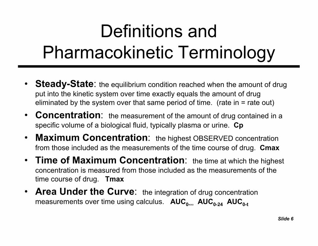
• Steady-State: the equilibrium condition reached when the amount of drug put into the kinetic system over time exactly equals the amount of drug eliminated by the system over that same period of time. (rate in = rate out)
• Concentration: the measurement of the amount of drug contained in a specific volume of a biological fluid, typically plasma or urine. Cp
• Maximum Concentration: the highest OBSERVED concentration from those included as the measurements of the time course of drug. Cmax
• Time of Maximum Concentration: the time at which the highest concentration is measured from those included as the measurements of the time course of drug. Tmax
• Area Under the Curve: the integration of drug concentration measurements over time using calculus. AUC0-∞ AUC0-24 AUC0-t

Slide 7
Key Pharmacokinetic Concepts• Key Pharmacokinetic Descriptive Variables
Half-Life, T½ Clearance, CL Volume of Distribution, V
• Primary Pharmacokinetic Measurements– Concentration (mass per volume), Cp– Rate constants (time-1), ka ke k12 λ β– Amount of Drug (mass), A Ae Dose– Area Under the Curve (integration of time and
mass per volume), AUC
CL = V ×××× 0.693 / T½
Slide 8
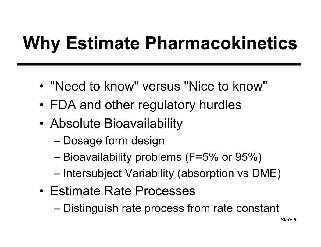
Why Estimate Pharmacokinetics
• "Need to know" versus "Nice to know"• FDA and other regulatory hurdles• Absolute Bioavailability
– Dosage form design– Bioavailability problems (F=5% or 95%)– Intersubject Variability (absorption vs DME)
• Estimate Rate Processes – Distinguish rate process from rate constant

Slide 9
Why Estimate Pharmacokinetics
• Characterize drug exposure – time duration– degree of exposure
• Predict dosage requirements– how much, how often
• Assess changes in dosage requirement– special populations– drug interactions
Slide 10
Why Estimate Pharmacokinetics
• Pharmacokinetic - PharmacodymamicRelationships– Concentration effect relationships– Use PK to provide concentration when PD
measurement is performed– Establish safety margins and efficacy
characteristics• Efficient and safe drug utilization

Slide 11
Pharmacokinetics
Pictorial and Graphical Understanding of the
Shapes of Concentration Time Profiles
Mathematical Models that describe and track these time profiles
Slide 12
Concentration profile depends on
• Route of Administration– Intravenous (bolus, infusion)– Extravascular (oral, IM, SQ)– Specialized
• Disposition of the drug (ADME)– distribution– metabolism– elimination

Slide 13
Pharmacokinetic Variability

Slide 14
IV BolusOne
Compartment

Slide 15
One Compartment Oral Administration

Slide 16
Effect of the Rate of Absorption
Rate of Absorptioncurve (fastest) 1 > 2 > 3 > 4 (slowest)
Ka Rate Constant (example)
0.1 0.01 0.001 0.0001 hr-1

Slide 17
Effect of Extent of Absorption
Hold Ka and Ke constantChange Bioavailability
(or dose)

Slide 18
Body Distribution Diagram One Compartment

Slide 19
Body Distribution Diagram Two Compartment
Slide 20
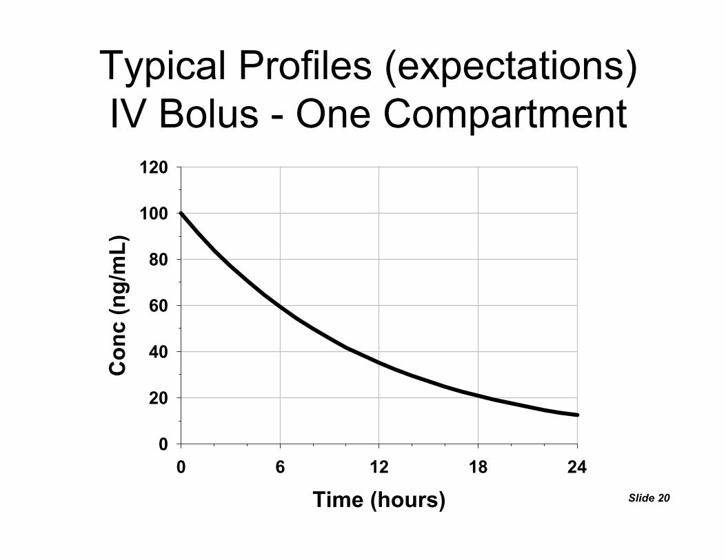
Typical Profiles (expectations)IV Bolus - One Compartment
Time (hours)0 6 12 18 24
Con
c (n
g/m
L)
0
20
40
60
80
100
120

Slide 21
Typical Profiles (expectations)IV Bolus - One Compartment
Time (hours)0 6 12 18 24
Con
c (n
g/m
L)
10
100

Slide 22
Typical Profiles (expectations)IV Bolus - Two Compartment
Time (hours)0 6 12 18 24
Con
c (n
g/m
L)
0
20
40
60
80
100
120
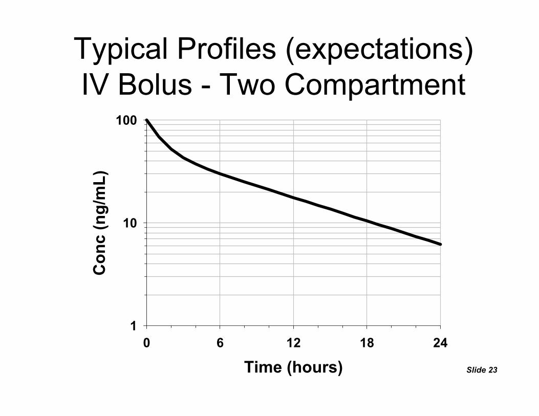
Slide 23
Typical Profiles (expectations)IV Bolus - Two Compartment
Time (hours)0 6 12 18 24
Con
c (n
g/m
L)
1
10
100

Slide 24
Typical Profiles (expectations)Oral - One Compartment
Time (hours)0 6 12 18 24
Con
c (n
g/m
L)
0
20
40
60
80
100

Slide 25
Typical Profiles (expectations)Oral - One Compartment
Time (hours)0 6 12 18 24
Con
c (n
g/m
L)
10
100

Slide 26
Typical Profiles (expectations)Oral - Two Compartment
Time (hours)0 6 12 18 24
Con
c (n
g/m
L)
0
20
40
60
80
100

Slide 27
Typical Profiles (expectations)Oral - Two Compartment
Time (hours)0 6 12 18 24
Con
c (n
g/m
L)
1
10
100

Slide 28
Noncompartmental PK AnalysisBASICS
• Gather Data - 3 Ds– Dosing, Demographic, Disposition
• Plot Data - (modeling step)– Observe any atypical features to note – Select the "terminal elimination" data / phase
• Perform Primary Calculations– Cmax, Tmax, AUC0-t, λz, AUC0-∞, Ae0-t, Ae0-∞,
AUMC0-t, AUMC0-∞
• Perform Secondary Calculations – CL, Vd, T½, MRT, MAT, Vdss, Ka, CLr, CLnr

Slide 29
Terminal Elimination Phase - Rate ConstantData Point Selection - β kel λz
• Customize for each individual and dose (treatment)
• Select from a semilog plot of conc vs time• Rough rules / helpful guidelines
– Number of selected data points ≥ 3– Avoid undue influence of any single point – "Omit" unruly data (undue influence)– Avoid influence of PK model (disposition), match
expectations– Document exact selection of data points

Slide 30
• Use linear regression of Ln(C) vs T– slope = terminal (elimination) rate constant
• Diagnostics Measures– goodness of fit measures – impact on PK analysis– impact on estimation of half-life– impact on extrapolation of AUC
Terminal Elimination Phase - Rate ConstantMethodology - β kel λz

Slide 31
• General Guidelines– AUCt-∞ - (extrapolated area) < 10% AUC0-∞
– Half-life is within timeframe of observations (NTL 1 half-life optimally 3 half-lives)
– Concentrations decline through at least one log cycle– Cmax at least 10x minimal measurable concentration– Reached point where measurements a BQL
• Does not violate basic modeling assumptions– linear pharmacokinetics– disposition described by first-order kinetics– adequately defined terminal log-linear elimination phase
Terminal Elimination Phase - Rate ConstantDiagnostics/General Rules - β kel λz

Slide 32
AUC Calculations and ReportingAUC0-t and AUC0-∞
Linear or Log-Linear Trapezoidal Rule from time 0 to the last measurable concentration.
Extrapolation from last measurable concentration to infinity
)t-(t)C(C 0.5 AUC i1i1i
1-n
1 iit0- ++
=
×+×= ∑
Z
last-t
^
-tC AUCλ
=∞
Regression line predicted concentration versus last observed concentration

Slide 33
Trapezoidal AUC

Slide 34
Steady-State versus Single DoseAUC0-tau versus AUC0-∞
Slide 35
Textbook Assignment:
Clinical Pharmacokinetics:Read Chapters 1, 2, 3, 4 Chapter 3: Problems 1, 2, 4, 5, 7, 8
Chapter 4: Problem 3
Homework for First Week


![Clinical Pharmacokinetics Samplechapter[1]](https://static.fdocuments.us/doc/165x107/577d34e41a28ab3a6b8f1c1d/clinical-pharmacokinetics-samplechapter1.jpg)