Atmos. Chem. Phys., 19, 7567–7581, 2019https://doi.org/10.5194/acp-19-7567-2019© Author(s) 2019. This work is distributed underthe Creative Commons Attribution 4.0 License.

Climatology of the mesopause relative density using a globaldistribution of meteor radarsWen Yi1,2, Xianghui Xue1,2,5, Iain M. Reid3,4, Damian J. Murphy6, Chris M. Hall7, Masaki Tsutsumi8, Baiqi Ning9,Guozhu Li9, Robert A. Vincent3,4, Jinsong Chen10, Jianfei Wu1,2, Tingdi Chen1,2, and Xiankang Dou1

1CAS Key Laboratory of Geospace Environment, Department of Geophysics and Planetary Sciences,University of Science and Technology of China, Hefei, China2Mengcheng National Geophysical Observatory, School of Earth and Space Sciences,University of Science and Technology of China, Hefei, China3ATRAD Pty Ltd., Thebarton, South Australia, Australia4School of Physical Sciences, University of Adelaide, Adelaide, South Australia, Australia5Synergetic Innovation Center of Quantum Information and Quantum Physics,University of Science and Technology of China, Hefei, China6Australian Antarctic Division, Kingston, Tasmania, Australia7Tromsø Geophysical Observatory, UiT – The Arctic University of Norway, Tromsø, Norway8National Institute of Polar Research, Tachikawa, Japan9Key Laboratory of Earth and Planetary Physics, Institute of Geology and Geophysics,Chinese Academy of Sciences, Beijing, China10National Key Laboratory of Electromagnetic Environment, China Research Institute of Radiowave Propagation,Qingdao, China

Correspondence: Xianghui Xue (xuexh@ustc.edu.cn) and Iain M. Reid (ireid@atrad.com.au)

Received: 30 September 2018 – Discussion started: 15 November 2018Revised: 19 May 2019 – Accepted: 23 May 2019 – Published: 6 June 2019

Abstract. The existing distribution of meteor radars locatedfrom high- to low-latitude regions provides a favorable tem-poral and spatial coverage for investigating the climatologyof the global mesopause density. In this study, we report theclimatology of the mesopause relative density estimated us-ing multiyear observations from nine meteor radars, namely,the Davis Station (68.6◦ S, 77.9◦ E), Svalbard (78.3◦ N,16◦ E) and Tromsø (69.6◦ N, 19.2◦ E) meteor radars lo-cated at high latitudes; the Mohe (53.5◦ N, 122.3◦ E), Bei-jing (40.3◦ N, 116.2◦ E), Mengcheng (33.4◦ N, 116.6◦ E) andWuhan (30.5◦ N, 114.6◦ E) meteor radars located in the mid-latitudes; and the Kunming (25.6◦ N, 103.8◦ E) and Darwin(12.3◦ S, 130.8◦ E) meteor radars located at low latitudes.The daily mean relative density was estimated using ambipo-lar diffusion coefficients derived from the meteor radars andtemperatures from the Microwave Limb Sounder (MLS) onboard the Aura satellite. The seasonal variations in the DavisStation meteor radar relative densities in the southern po-

lar mesopause are mainly dominated by an annual oscilla-tion (AO). The mesopause relative densities observed by theSvalbard and Tromsø meteor radars at high latitudes and theMohe and Beijing meteor radars at high midlatitudes in theNorthern Hemisphere show mainly an AO and a relativelyweak semiannual oscillation (SAO). The mesopause relativedensities observed by the Mengcheng and Wuhan meteorradars at lower midlatitudes and the Kunming and Darwinmeteor radars at low latitudes show mainly an AO. The SAOis evident in the Northern Hemisphere, especially at high lat-itudes, and its largest amplitude, which is detected at theTromsø meteor radar, is comparable to the AO amplitudes.These observations indicate that the mesopause relative den-sities over the southern and northern high latitudes exhibit aclear seasonal asymmetry. The maxima of the yearly varia-tions in the mesopause relative densities display a clear lati-tudinal variation across the spring equinox as the latitude de-creases; these latitudinal variation characteristics may be re-

Published by Copernicus Publications on behalf of the European Geosciences Union.

7568 W. Yi et al.: Climatology of the mesopause relative density

lated to latitudinal changes influenced by gravity wave forc-ing. In addition to an AO, the mesopause relative densitiesover low latitudes also clearly show an intraseasonal varia-tion with a periodicity of 30–60 d.

1 Introduction

The temperatures, winds and densities in the mesopause re-gion are essential for studying the dynamics and climate, in-cluding both short-term wave motions (e.g., gravity waves,tides and planetary waves) and long-term climate varia-tions (e.g., interannual variations, seasonal variations andintraseasonal variations), of the middle and upper atmo-sphere. The climatology of the temperature and wind withinthe mesopause region has been studied for decades usingground-based instruments such as meteor radars, medium-frequency (MF) radars, lidars (Dowdy et al., 2001; Dou et al.,2009; Li et al., 2008, 2012, 2018) and satellite instruments(Garcia et al., 1997; Remsberg et al., 2002; Xu et al., 2007).It is well established that the semiannual oscillation (SAO)dominates the seasonal variations in both the wind and thetemperature in the low-latitude mesosphere (Li et al., 2012),whereas the annual oscillation (AO) dominates the seasonalvariations in the mid- and high-latitude mesosphere (Rems-berg et al., 2002; Xu et al., 2007; Dou et al., 2009). How-ever, in contrast to temperature and wind observations, long-term continuous measurements of the atmospheric density inthe mesopause region are still quite rare; as a result, the sea-sonal variations in the mesopause, especially with regard toits global structure, are still unclear.

Meteor radar operates both day and night under all kindsof weather and geographical conditions and provides goodlong-term observations; consequently, meteor radar is a pow-erful technique for studying the dynamics and climate of themesopause region, including its wind fields and temperatures(e.g., Hocking et al., 2004; Holdsworth et al., 2006; Hall etal., 2006, 2012; Stober et al., 2008, 2012; Yi et al., 2016;Lee et al., 2016; Holmen et al., 2016; Liu et al., 2017; Limaet al., 2018; Ma et al., 2018). In addition to acquiring windand temperature measurements, meteor radar has also beenapplied in recent years to estimate the atmospheric densityin the mesopause region. For instance, the variation in thepeak height of meteor radar detections can be used to esti-mate changes in the mesopause density (e.g., Clemesha andBatista, 2006; Stober et al., 2012, 2014; Lima et al., 2015;Liu et al., 2016). However, the seasonal variations in the peakheight are not affected by the atmospheric density alone; theyare also significantly influenced by the properties of mete-oroids, especially the meteor velocity (Stober et al., 2012;Yi et al., 2018b). Furthermore, the mesospheric densities canalso be estimated from meteor-radar-derived ambipolar dif-fusion coefficients, and the mesospheric temperatures canbe derived from other measurements (e.g., Takahashi et al.,

2002; Yi et al., 2018b). Therefore, in this study, we applyambipolar diffusion coefficients derived from a global dis-tribution of meteor radars in addition to temperature mea-surements simultaneously obtained by the Microwave LimbSounder (MLS) on board the Aura satellite to determine themesopause relative density. In addition, long-term observa-tions of global atmospheric densities are used to study thelatitudinal and seasonal variations in the mesopause region.Descriptions of the instrument datasets, the method, and theerror estimation approach are presented in Sect. 2. Then, theseasonal variations in the mesopause density are presented inSect. 3, followed by a composite analysis in Sect. 4. Finally,a summary is provided in Sect. 5.

2 Data and methods

In this study, data from nine meteor radars, namely, theDavis Station (68.6◦ S, 77.9◦ E), Svalbard (78.3◦ N, 16◦ E),Tromsø (69.6◦ N, 19.2◦ E), Mohe (53.5◦ N, 122.3◦ E), Bei-jing (40.3◦ N, 116.2◦ E), Mengcheng (33.4◦ N, 116.5◦ E),Wuhan (30.6◦ N, 114.4◦ E), Kunming (25.6◦ N, 108.3◦ E)and Darwin (12.3◦ S, 130.5◦ E) meteor radars (hereinafter re-ferred to as DMR, SMR, TMR, MMR, BMR, McMR, WMR,KMR and DwMR, respectively), were used. Table 1 summa-rizes the operational frequencies, geographic locations andobservational time periods for the meteor radars used in thisstudy. These meteor radars all belong to the ATRAD meteordetection radar (MDR) series and are similar to the Buck-land Park meteor radar system described by Holdsworth etal. (2004). Figure 1 shows the locations of these nine meteorradars. The SMR and TMR are located in the northern highlatitudes, whereas the MMR, BMR, McMR and WMR arepositioned in the northern midlatitudes, and the KMR is sit-uated in the northern low latitudes. In contrast, we have onlytwo meteor radars, namely, the DMR located in the southernhigh latitudes and the DwMR situated in the southern lowlatitudes, in the Southern Hemisphere because it is coveredprimarily by oceans.

The ambipolar diffusion coefficient (Da) observed by ameteor radar describes the rate at which plasma diffuses in aneutral background and is a function of both the atmospherictemperature, T , and the atmospheric density, ρ, as given by

ρ = 2.23× 10−4K0T

Da, (1)

where K0 is the ionic zero-field mobility, which is assumedto be 2.5× 10−4 m−2 s−1 V−1 (Hocking et al., 1997). Usingthe relation given by Eq. (1), measurements of the temper-ature and Da from meteor radars can be used to retrieve theneutral mesospheric density (see, e.g., Takahashi et al., 2002;Yi et al., 2018b).

The MLS instrument on board the Earth Observing Sys-tem (EOS) Aura spacecraft was launched in 2004. For thisinvestigation, the Aura MLS temperature (Schwartz et al.,

Atmos. Chem. Phys., 19, 7567–7581, 2019 www.atmos-chem-phys.net/19/7567/2019/

W. Yi et al.: Climatology of the mesopause relative density 7569

Table 1. Main operation parameters, geographic coordinates and observational time periods for the meteor radars used in this study.

Meteor radar Geographic coordinates Frequency Data used in this study

Northern Hemisphere

Svalbard (SMR) 78.3◦ N, 16◦ E 31 MHz Jan 2005–Dec 2016Tromsø (TMR) 69.6◦ N, 19.2◦ E 30.3 MHz Jan 2005–Dec 2016Mohe (MMR) 53.5◦ N, 122.3◦ E 38.9 MHz Aug 2011–Apr 2018Beijing (BMR) 40.3◦ N, 116.2◦ E 38.9 MHz Jan 2011–Apr 2018Mengcheng (McMR) 33.4◦ N, 116.5◦ E 38.9 MHz Sep 2014–Apr 2018Wuhan (WMR) 30.6◦ N, 114.4◦ E 38.9 MHz Oct 2012–Aug 2017Kunming (KMR) 25.6◦ N, 108.3◦ E 37.5 MHz Apr 2011–Dec 2014

Southern HemisphereDavis (DMR) 68.6◦ S, 77.9◦ E 33.2 MHz Jan 2005–Dec 2016Darwin (DwMR) 12.3◦ S, 130.5◦ E 33.2 MHz Jan 2006–Dec 2009

Figure 1. The locations of the meteor radars used in this study.

2008) and geopotential height data (version 4) were re-stricted to data obtained within a 10◦× 20◦ bounding boxcentered on each of the abovementioned meteor radar loca-tions. Geometric heights, z, for Aura MLS observations werecomputed from geopotential heights, zg, via the equationz= zgRE (φ) [RE (φ)− zg]

−1 (Younger et al., 2014), whereRE (φ) is the radius of Earth at latitude φ, based on theWGS84 ellipsoid (Decker, 1986). The daily averaged MLStemperature and geometric height observations were interpo-lated into 1 km bins between 85 and 95 km to produce tem-perature profiles.

In this study, in order to avoid the possibility of excessiveerror in the height estimates of individual meteors, trail de-tections for this study were restricted to zenith angles of lessthan 60◦. All meteor radars in this study transmit a 3.6 kmlong, 4 bit complimentary coded pulse with a pulse repeti-tion frequency (PRF) of 430 Hz, so the meteor radar rangesampling resolution is 1.8 km (Holdsworth et al., 2008). With

the criterion of zenith < 60◦, the meteor height estimate un-certainty (range sampling resolution× cos(zenith)) should beless than ±1 km. The daily neutral mesospheric densitiesfrom 85 to 95 km were estimated using the daily mean Dafrom the nine meteor radars and the Aura MLS temperaturesusing Eq. (1); more details are described by Yi et al. (2018b).Yi et al. (2018b) showed that the log10Da profiles derivedfrom meteor radars are approximately linear with respectto the altitude in the range from 85 to 95 km, which indi-cates that mainly ambipolar diffusion governs the evolutionof meteor trails in this region. In general, the log10Da pro-files measured by meteor radars have larger slopes than thosederived from Sounding of the Atmosphere using BroadbandEmission Radiometry (SABER) (Yi et al., 2018b) and MLS(Younger et al., 2015) measurements. To avoid the influenceof the bias inDa, in the present study, we use the relative vari-ation in the density to examine the climatology of the globalmesopause density.

There is an uncertainty in Da caused by the estimation ofthe decay time of meteor echoes (e.g., Cervera and Reid,2000; Holdsworth et al., 2004); unfortunately, this uncer-tainty is quite difficult to estimate from the radar system di-rectly. In addition, the number of precise, simultaneously ob-served temperature and density measurements in the studyregion is insufficient to estimate the absolute error in Dathrough a comparison. Yi et al. (2018b) compared simulta-neous observations of Da acquired by two co-located me-teor radars at Kunming and found that the relative errors inthe daily mean Da and the density at 90 km obtained fromthe KMR should be less than 5 % and 6 %, respectively.Here, to estimate the relative errors in Da and the density,we conduct a similar approach using simultaneous meteorechoes observed by two co-located meteor radars with dif-ferent frequencies (33 and 55 MHz) at Davis Station. The 33and 55 MHz meteor radars at Davis Station are described inrelated studies (see, e.g., Reid et al., 2006; Younger et al.,2014).

Figure 2a shows the height distributions of meteor detec-tions in 1 km bins on 1 January and 1 July 2006 for the 33 and55 MHz meteor radars at Davis Station. The meteor count ob-

www.atmos-chem-phys.net/19/7567/2019/ Atmos. Chem. Phys., 19, 7567–7581, 2019

7570 W. Yi et al.: Climatology of the mesopause relative density

Figure 2. (a) The height distributions of meteor detections in 1 km bins on 1 January and 1 July 2006 from the 33 and 55 MHz meteor radarsat Davis Station. (b) Height variation in the correlation coefficient between the Da observed simultaneously by the 33 and 55 MHz meteorradars at Davis Station in 2006. The error bars indicate the lower and upper bounds of the 95 % confidence interval for each coefficient.(c) Comparison of the variations in the daily mean Da (blue dots) at 90 km simultaneously observed from the 33 and 55 MHz meteor radarsat Davis Station in 2006. The percentage variations in Da with respect to the yearly mean Da in 2006. N represents the number of daysobserved by these two radars in 2006, and R denotes the linear correlation coefficient.

served by the 55 MHz meteor radar is much lower than thatobserved by the 33 MHz meteor radar because the formeris a mesosphere–stratosphere–troposphere (MST) radar op-erating with time-interleaved stratosphere–troposphere (ST),meteor and polar mesosphere summer echoes (PMSE) modes(see, e.g., Reid et al., 2006). Figure 2b shows the correlationcoefficients between the Da observed simultaneously by thetwo co-located meteor radars from 85 to 95 km. The correla-tion coefficients are higher than 0.96 below 92 km, and theybecome lower as the altitude increases above 92 km; this oc-curs mainly because the meteor count (as shown in Fig. 2a)obtained by the 55 MHz meteor radar above 92 km is too lowto provide a good precision inDa. The strong correlation be-tween the Da measurements from the two independent me-teor radars indicates that the variations in Da are dominatedby the same geophysical variations (i.e., gravity waves, tidesand planetary waves) from below as well as by disturbancesby geomagnetic forcing from above (Yi et al., 2017, 2018a)rather than by random systemic errors; therefore, the differ-ence between the two Da measurements is considered to berepresentative of the relative uncertainty in Da.

The MLS temperature has an accuracy of 1–3 K from 316to 0.001 hPa (Schwartz et al., 2008). The vertical resolutionof MLS measurements near the mesopause region (about90 km) is ∼ 3–4 km. This may introduce a bias betweenthe interpolated temperatures and the actual mesopause tem-peratures because of the reversal temperature gradient inthe mesopause region. In order to estimate the uncertaintiescaused by the temperature interpolation, we also compared

the relative the interpolated MLS temperatures between theSABER temperatures over the Mohe meteor radar. The rel-ative uncertainty in the density induced by the interpolatedMLS temperature uncertainty would be less than 3 % basedon the present values. Comprehensive consideration in Ta-ble 2 shows a summary of the relative uncertainties in thedensity from 85 to 95 km. The relative density uncertaintiesare less than 6 % below 92 km and become larger as the alti-tude increases above 92 km. However, under real-world con-ditions, the meteor counts from the nine meteor radars usedin this study are much larger than those from the 55 MHz me-teor radar, and, hence, it is reasonable to believe that the un-certainties in the relative density above 92 km would be lowerthan this estimate of 6 %. The density scale height near 90 kmover the Mohe meteor radar is approximately 6 km, whichmeans an increase of 1 km in geometric height would cor-respond to a density decrease of approximately 17 %, whichmay indicate that the relatively uncertainty of the density es-timation is much smaller than 1 km.

3 Seasonal variations in the global mesopause relativedensity

Figure 3 shows the monthly mean mesopause relative densi-ties in the southern polar region derived from the DMR andin the northern polar region derived from the SMR and TMRbetween 2005 and 2016. As shown in Fig. 3a, the DMR rela-tive densities are dominated by an AO with a maximum dur-ing the spring and a minimum during the early winter. The

Atmos. Chem. Phys., 19, 7567–7581, 2019 www.atmos-chem-phys.net/19/7567/2019/

W. Yi et al.: Climatology of the mesopause relative density 7571

Table 2. The relative uncertainties in Da and the density from 85 to 95 km.

Altitude (km) 85 86 87 88 89 90 91 92 93 94 95

Relative uncertainties in Da (%) 3 2 2 2 2 3 4 6 11 18 24Relative uncertainties in the density (%) 4.2 3.6 3.6 3.6 3.6 4.2 5.2 6.7 11.4 18.2 24.2

annual variations in the DMR relative densities are approxi-mately 65 % of the mean density. Younger et al. (2015) devel-oped a novel technique using meteor radar echo decay timesfrom the DMR to determine the height of a constant-densitysurface in the mesopause region and found that the height ofthe constant-density surface is also dominated by an AO. Inthe northern polar region, the SMR relative densities mainlyshow an AO and a relatively weak SAO with a clear max-imum during the spring. However, the minima of the SMRrelative densities are not as regular as the DMR relative den-sities, and they appear approximately during the summer andwinter. The TMR relative densities mainly show an AO andSAO with a clear maximum during the spring and two dis-tinct minima during the summer and winter. As the SMR andTMR are in the northern polar region, the SMR and TMRrelative densities show a similar annual variation; however,the semiannual variations in the TMR relative densities aremore obvious than those of the SMR relative densities.

To further examine the periodicities present in themesopause relative densities derived from the meteor radars,Lomb–Scargle periodograms were calculated for the entireobservational period of the densities in each 1 km bin from 85to 95 km. Figure 4 shows the contours of the Lomb–Scargleperiodograms of the mesopause relative densities obtainedfrom the DMR, SMR and TMR. The periodograms of theDMR relative densities in Fig. 4a are clearly dominated by anAO as well as a relatively weak SAO; the largest amplitude ofthe AO appears at 87 km, where it is 20 % of the mean DMRdensities. The periodograms of the SMR relative densitiesmainly show an AO and SAO, and the amplitudes of the AOand SAO at 90 km are approximately 12 % and 8 %, respec-tively, of the mean SMR densities. The TMR mainly showsan AO and SAO, and the amplitudes of the AO and SAO at90 km are approximately 11 % and 10 %, respectively. In ad-dition to an AO and SAO, the northern polar mesosphericdensities from the SMR and TMR also exhibit clear seasonalperiodicities with quasi-120 d and quasi-90 d oscillations.

Figure 5 shows the monthly mean mesospheric relativedensities at northern midlatitudes derived from the MMR,BMR, McMR and WMR. The MMR monthly mean rela-tive densities (Fig. 5a) from August 2012 to April 2018 athigher midlatitudes clearly show both an AO and an SAO;the AO clearly reaches a maximum in the spring (April),whereas the SAO shows two distinct minima: one clearly ap-pears in the summer above 90 km, and another clearly ap-pears in the winter below 90 km. As shown in Fig. 5b, theBMR monthly mean relative densities from January 2011

to April 2018 show mainly an AO with a maximum duringthe spring and a minimum during the summer. The McMRmonthly mean relative densities (Fig. 5c) from October 2014to April 2018 show seasonal variations similar to those ex-hibited by the BMR relative densities with a clear minimumduring the summer and a maximum during the spring. Asshown in Fig. 5d, the WMR monthly mean relative densi-ties from October 2012 to September 2017 show mainly anAO with a maximum during the late winter and a minimumduring the summer. As the WMR is located close to the lowlatitudes, the annual variations in the WMR relative densi-ties are much smaller than those in the densities observed bymeteor radars at high latitudes and higher midlatitudes.

Figure 6 displays the contours of the Lomb–Scargle pe-riodograms of the mesopause relative densities from theMMR, BMR, McMR and WMR. The MMR relative densi-ties (Fig. 6a) show mainly an AO and SAO; the amplitudesof the AO reach a maximum at 87 km, where the amplitudeis approximately 8 % of the MMR mean densities, while theamplitudes of the SAO are larger than those of the AO above90 km with a maximum that is approximately 7 % of theMMR mean densities at 93 km. The BMR and McMR rel-ative densities (Fig. 6b and c, respectively) show similar pe-riodograms; they exhibit mainly an AO and a relatively weakSAO. In contrast, the WMR relative densities are dominatedby an AO above 89 km; however, below 89 km, they showboth an SAO and an AO.

Figure 7a shows the KMR monthly mean relative densi-ties in the northern low latitudes from April 2011 to Decem-ber 2014. The KMR relative densities show mainly an AOwith a maximum during the winter and a minimum duringthe summer. Figure 7b shows the DwMR relative densitiesat southern low latitudes from January 2006 to June 2009.The DwMR relative densities exhibit a large data gap; how-ever, the data still provide the opportunity to investigate theclimatology of the mesospheric density at southern low lat-itudes. The seasonal variations in the DwMR relative den-sities are more complicated than those in the KMR relativedensities and clearly show intraseasonal (with a periodicityof 30–60 d) oscillations. To more clearly examine the sea-sonal variations in the mesospheric densities, Fig. 8 showsthe Lomb–Scargle periodograms of the KMR and DwMRrelative densities. The largest component of the KMR rela-tive densities is an AO above 87 km, followed by an SAO, a90 d oscillation and a 60 d oscillation; below 87 km, the SAObecomes more obvious in the KMR relative densities, whichcan also be seen in Fig. 7a. The DwMR relative densities

www.atmos-chem-phys.net/19/7567/2019/ Atmos. Chem. Phys., 19, 7567–7581, 2019

7572 W. Yi et al.: Climatology of the mesopause relative density

Figure 3. Variations in the monthly mean relative densities at altitudes from 85 to 95 km obtained from the DMR, SMR and TMR between2005 and 2016. The color bars indicate the percentage variation in the monthly mean density relative to the mean density from the totalobservational time period.

Figure 4. Contours of the Lomb–Scargle spectral (see, e.g., Lomb, 1976; Scargle, 1982) relative amplitudes of the (a) DMR, (b) SMR and(c) TMR densities. The white lines represent the 99 % significance level.

show both an AO and an SAO above 92 km. In addition toseasonal variations, the DwMR relative densities also exhibitbroad oscillations with periodicities ranging from 30 to 60 d;these periodic variations may be similar to intraseasonal os-cillations (Eckermann and Vincent, 1994).

4 Composite analysis for the global mesopause relativedensity

In the results described above, we presented the year-to-yearvariability in the climatology of the global mesopause rela-tive density. To better appreciate the latitudinal changes ofthe seasonal variations in the global mesopause relative den-sity, we show a composite analysis for the nine meteor radar

Atmos. Chem. Phys., 19, 7567–7581, 2019 www.atmos-chem-phys.net/19/7567/2019/

W. Yi et al.: Climatology of the mesopause relative density 7573

Figure 5. Same as Fig. 3 but for the MMR, BMR, McMR and WMR monthly mean relative densities.

Figure 6. Same as Fig. 4 but for the MMR, BMR, McMR and WMR daily mean relative densities in the midlatitudes.

www.atmos-chem-phys.net/19/7567/2019/ Atmos. Chem. Phys., 19, 7567–7581, 2019

7574 W. Yi et al.: Climatology of the mesopause relative density

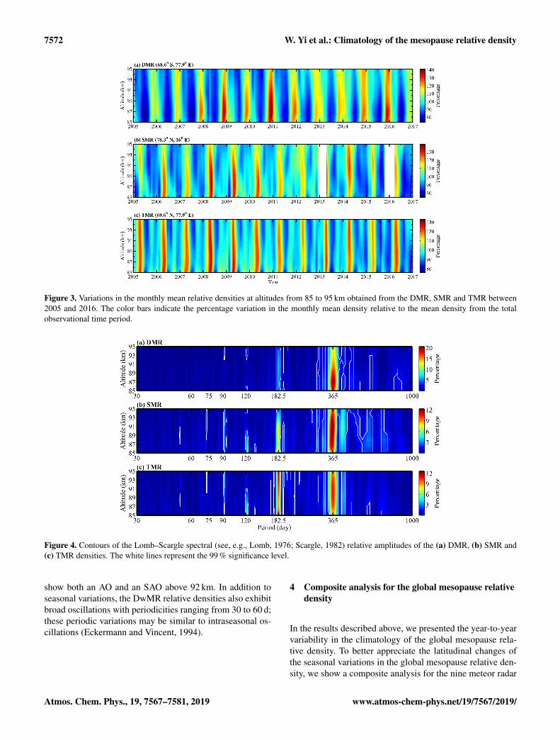
Figure 7. Same as Fig. 3 but for the KMR and DwMR monthly mean relative densities at low latitudes.

Figure 8. Same as Fig. 4 but for the KMR and DwMR daily mean relative densities at low latitudes.

measurements in Fig. 9. For this composite analysis, we firstcombine the nine meteor radar relative densities into a singleyear and then use a 30 d running average to obtain the sea-sonal variations in the global mesopause relative density. Asshown in Fig. 9, several distinct features are present in theclimatology of the global mesopause relative density.

It is clear that the seasonal variations in the mesopauserelative densities exhibit latitudinal differences. The seasonalvariations in the mesopause relative densities obtained fromthe SMR and TMR at northern high latitudes and the MMRat higher northern midlatitudes are similar; they display a pri-mary maximum after the spring equinox and a minimum dur-ing the summer. In the northern midlatitudes, the mesopauserelative densities from the BMR, McMR and WMR exhibitsimilar seasonal variations with a strong maximum near thespring equinox, a weak maximum before the winter solsticeand a minimum during the summer. As shown in Fig. 9, the

most noticeable feature is that the temporal evolution of themaximum mesopause relative density shifts as the latitudechanges. For instance, the phase of the maximum shifts fromspring (May) to winter (January) across the spring equinoxfrom the high latitudes to the low latitudes in the North-ern Hemisphere. Referring to the recent studies by Jia etal. (2018) and Ma et al. (2018), a similar feature was alsopresent in the zonal mean winds simultaneously observed bythe MMR, BMR, McMR and WMR at northern midlatitudes;they reported that the zonal winds above 85 km generally ex-hibit an annual variation with a maximum during the sum-mer (eastward), and they further demonstrated that the windshifts (i.e., the zero zonal wind) near the spring equinox. Inaddition, based on their results, we also find that the phase ofthe maximum in the zonal wind also shifts as the latitude de-creases; meanwhile, the time at which the zonal wind shiftsalso demonstrates a transition across the spring equinox from

Atmos. Chem. Phys., 19, 7567–7581, 2019 www.atmos-chem-phys.net/19/7567/2019/

W. Yi et al.: Climatology of the mesopause relative density 7575

Figure 9. Contours of the composite 30 d running mean values of the mesopause densities in the composite year from the North Pole to theSouth Pole observed by the (a) SMR, (b) TMR, (c) MMR, (d) BMR, (e) McMR, (f) WMR, (g) KMR, (h) DwMR and (i) DMR. The dashedlines indicate the spring and autumn equinoxes and the summer and winter solstices. The color bars indicate the percentage variation in the30 d running mean density relative to the mean density from the total observational time period.

the MMR to the WMR, which is similar to the observedmesopause relative densities shown in Fig. 9.

It is also worth noting that the minima of the globalmesopause relative densities appear during June, July andAugust. The minima of the northern polar mesopause rela-

tive densities obtained from the SMR and TMR occur duringthe Northern Hemisphere summer, while the DMR relativedensities also show minima during the Southern Hemispherewinter. The mesopause relative densities over the northernmidlatitudes obtained from the MMR, BMR, McMR and

www.atmos-chem-phys.net/19/7567/2019/ Atmos. Chem. Phys., 19, 7567–7581, 2019

7576 W. Yi et al.: Climatology of the mesopause relative density

WMR all appear during the Northern Hemisphere summer.Because no measurements of the mesopause relative densityover the southern midlatitudes are presented in this study, wecannot provide a comparison for the interhemispheric midlat-itudes. With regard to the low latitudes, the mesopause rela-tive densities obtained from the KMR clearly show a mini-mum during the Northern Hemisphere summer above 87 km.In contrast, the DwMR relative densities in the southern lowlatitudes show a clear minimum during August and Septem-ber, which is not during the expected Southern Hemispheresummer. These results reveal a seasonal asymmetry in themesopause relative density in both hemispheres. During theNorthern Hemisphere summer (the perihelion is on 4 July),the distance between the Sun and the Earth is 3.3 % longerthan that during the Northern Hemisphere winter (the aphe-lion is on 3 January); therefore, the longer distance betweenthe Sun and the Earth during the Northern Hemisphere sum-mer leads to a reduction of 6.7 % in the total solar radia-tion absorbed by the Earth, causing the Earth’s atmosphere toshrink. This may explain why the global mesopause relativedensities show a minimum during the Northern Hemispheresummer.

Figure 10 shows the harmonic fitting results for the com-posite global mesopause relative density (shown in Fig. 9).As shown in Fig. 10a, it is clear that the AO displays largeamplitudes exceeding 10 % at high latitudes (DMR, SMRand TMR); the maxima of the AO amplitudes observed bythe DMR, SMR and TMR reach 21 %, 13 % and 12 %, re-spectively. Moreover, the amplitudes of the AO at southernhigh latitudes (DMR) are much larger than those at northernhigh latitudes (SMR and TMR). In the midlatitudes (MMR,BMR, McMR and WMR), the AO amplitudes observed bythe McMR are stronger than those observed by the otherthree stations, especially the MMR and BMR situated in thehigher midlatitudes. At low latitudes, the AO observed by theKMR is stronger than that observed by the DwMR at lowerlatitudes in the Southern Hemisphere as well as that observedby the WMR at higher latitudes.

Similarly, Fig. 10b shows the SAO amplitudes observed bythe nine meteor radars; the SAO is much weaker than the AO,as shown in Fig. 10a. It is clear that the SAO is strongest atthe TMR and that the amplitudes are comparable to those ofthe AO with a mean of approximately 10 %. The SAOs in thenorthern high latitudes (SMR and TMR) are stronger thanthose in the southern high latitudes (DMR). In the midlati-tudes (MMR, BMR, McMR and WMR), the amplitudes ofthe SAOs decrease as the latitude decreases and roughly in-crease with decreasing altitude. The SAOs are much weakerin the low latitudes (KMR and DwMR), which is differentfrom the temperature and horizontal wind in the low-latitudemesopause. The SAO is clearly the dominant seasonal vari-ation in both the horizontal wind (Li et al., 2012) and thetemperature (Xu et al., 2007) in the mesosphere at low lat-itudes. This might be because the seasonal variations in themesopause density are influenced by the atmospheric dynam-

ics as well as atmospheric equilibrium; however, this rela-tionship is too complicated to understand at the moment.

Figure 10c and d show the phases of the AO and SAO, re-spectively, observed by the nine meteor radars. The phasesof the AO show an approximately decreasing trend as the lat-itude decreases and a downward progression as the altitudeincreases. In addition, the phases of the SAO clearly showa decreasing trend from the high latitudes (SMR) to the lowlatitudes (KMR); this can also explain the shift in the tem-poral evolution of the mesopause density maxima as the lat-itude changes. The times at which the density maxima occur(Fig. 9) are consistent with the phases of the SAO shown inFig. 10d. In addition, the phases of the SAO observed by theWMR, KMR and DwMR show a phase shift as the altitudeincreases; this is also reflected in Fig. 9. Placke et al. (2011)and Jia et al. (2018) calculated the gravity wave momen-tum fluxes in the mesosphere and lower thermosphere us-ing the meteor radars at Collm, Germany (51.3◦ N, 13.0◦ E),as well as Mohe and Beijing; they reported that the grav-ity wave variations exhibit an SAO at an altitude of approx-imately 90 km with a maximum during the summer and asecondary, weaker maximum during the winter as well astwo minima around the equinoxes. Furthermore, Dowdy etal. (2001) suggested that radiative effects are stronger in theSouthern Hemisphere and that gravity wave driving effectsare more important in the Northern Hemisphere. These re-sults may explain why the SAOs are more obvious at theSMR and TMR at high latitudes and at the MMR and BMRat higher midlatitudes as well as why the SAO at northernhigh latitudes is stronger than that at southern high latitudes.

Figure 11 shows a comparison of the climatology of themesopause relative density at 90 km in the composite yearamong the meteor radars in addition to the mesopause rela-tive densities calculated simultaneously by the US Naval Re-search Laboratory Mass Spectrometer and Incoherent Scatter(NRLMSISE-00) model (Picone et al., 2002) and Whole At-mosphere Community Climate Model version 4 (WACCM4).The WACCM is an atmospheric component of the Commu-nity Earth System Model (CESM) version 1.0.4 developedby the National Center for Atmospheric Research; the keyfeatures are described in detail in Marsh et al. (2013). Inaddition, the WACCM is a superset of the Community At-mospheric Model version 4 with 66 vertical hybrid levelsfrom the surface to the lower thermosphere (∼ 145 km); thevertical spacing increases with the altitude from ∼ 1.1 kmin the troposphere to 1.1–1.8 km in the lower stratosphereand 3.5 km above ∼ 65 km. The horizontal resolution for theWACCM4 used here is 1.9◦ latitude by 2.5◦ longitude.

The comparisons shown in Fig. 11 reveal evident differ-ences between the observations and models. The MSIS rela-tive densities show a dominant AO, the amplitude of whichdecreases as the latitude decreases. In the southern high lat-itudes, the MSIS relative densities generally exhibit an an-nual variation similar to those displayed by the DMR obser-vations with a maximum during November and December

Atmos. Chem. Phys., 19, 7567–7581, 2019 www.atmos-chem-phys.net/19/7567/2019/

W. Yi et al.: Climatology of the mesopause relative density 7577

Figure 10. Amplitudes (a, b) and phases (c, d) of the AO and SAO observed by the nine meteor radars. The amplitude values indicate thepercentage of the density relative to the mean density from the total observational time period.

and a minimum during July, but the AO shows a larger vari-ation than do the DMR observations. In the Northern Hemi-sphere from the SMR to the McMR, the difference betweenthe meteor radar observations and the MSIS model is obvi-ous because the SAOs in the meteor radar observations arestrong at these latitudes, while the SAO amplitude is muchweaker in the MSIS model. At lower latitudes, the MSIScaptures only the annual variations in the WMR, KMR andDwMR observations but fails to reproduce the other seasonaland intraseasonal variations. The WACCM relative densitiesshow mainly annual and semiannual variations but almostfail to capture the seasonal variations in the mesopause den-sity. However, it is worth noting that the WACCM relativedensities show a minimum during June, July and August; thisfeature is similar to the meteor radar observations. The com-parison between the observations and models demonstratesobvious inconsistencies, which indicate some limitations ofthe current models, such as the MSIS model and WACCM,regarding the seasonal behavior of the mesopause relativedensity.

The MSIS model is an empirical atmospheric model basedon observations acquired over a decade ago; in particular,mesospheric density data were quite scarce at that time,which is the likely reason that the MSIS model exhibits ob-vious differences from the meteor radar observations. More-over, the WACCM cannot directly provide atmospheric den-sity estimates. Hence, in this study, we calculate the WACCMdensity at 90 km using the WACCM-simulated temperatureand the geographic height corresponding to the pressurelevel. Previous studies indicated that WACCM-simulatedtemperatures are generally higher than lidar observations, but

the WACCM temperatures can reproduce the major featuresof the climatology of the mesopause temperatures (see, e.g.,Li et al., 2018). The accuracy of the pressure level (i.e., geo-graphic height) is quite difficult to estimate because of thelack of corresponding observations. This study constitutesthe first time we have compared the mesopause density simu-lated by the WACCM with meteor radar observations; hence,the remarkable differences in the seasonal variations betweenthem are difficult to understand at the moment and are be-yond the scope of this study.

5 Summary

Mesopause relative densities determined with data from aglobal distribution of meteor radars are used to investi-gate the climatology of the global mesopause relative den-sity. The multiyear observations of the mesopause rela-tive density involved nine meteor radars, namely, the DavisStation (68.6◦ S, 77.9◦ E), Svalbard (78.3◦ N, 16◦ E) andTromsø (69.6◦ N, 19.2◦ E) meteor radars located at highlatitudes; the Mohe (53.5◦ N, 122.3◦ E), Beijing (40.3◦ N,116.2◦ E), Mengcheng (33.4◦ N, 116.6◦ E) and Wuhan(30.5◦ N, 114.6◦ E) meteor radars located in the midlati-tudes; and the Kunming (25.6◦ N, 103.8◦ E) and Darwin(12.4◦ S, 130.8◦ E) meteor radars located at low latitudes.The mesopause relative densities estimated from these ninemeteor radars exhibit different seasonal and latitudinal vari-ations. The main points of the latitudinal and seasonal vari-ations in the mesopause relative density are summarized asfollows:

www.atmos-chem-phys.net/19/7567/2019/ Atmos. Chem. Phys., 19, 7567–7581, 2019

7578 W. Yi et al.: Climatology of the mesopause relative density

Figure 11. Comparisons of the mesopause relative densities at 90 km in the composite year among the meteor radars (solid red lines),the Mass Spectrometer and Incoherent Scatter (MSIS) model (solid blue lines) and the Whole Atmosphere Community Climate Model(WACCM) (solid green lines). The shaded areas represent the 30 d running averages and standard deviations of the composite density.

Atmos. Chem. Phys., 19, 7567–7581, 2019 www.atmos-chem-phys.net/19/7567/2019/

W. Yi et al.: Climatology of the mesopause relative density 7579

1. In the southern high latitudes, the AO observed by theDMR dominates the seasonal variations with a maxi-mum during the late spring and a minimum during theearly winter. In the Northern Hemisphere from high tolow latitudes (from the SMR to the KMR), the AOsdominate the seasonal variations in the mesopause rela-tive densities, and the amplitudes decrease equatorward.In addition to AOs, SAOs are also evident in the North-ern Hemisphere, especially at high latitudes, and theirlargest amplitude, which is detected at the TMR, is com-parable to the AO amplitudes. Near the Equator, themesopause relative densities observed by the DwMRshow an AO and relatively weak intraseasonal oscilla-tions with a periodicity of 30–60 d.

2. Interhemispheric observations indicate that themesopause relative densities over the southern andnorthern polar regions show a clear seasonal asym-metry. The maxima of the yearly variations in themesopause relative density exhibit a clear temporalvariation across the spring equinox as the latitudedecreases; these latitudinal variation characteristicsmay be related to the latitudinal variation in the globalcirculation of the mesosphere influenced by gravitywave forcing. In addition, the minima of the globalmesopause relative densities basically appear duringJune, July and August. A possible explanation for thisphenomenon is that the longer distance between theSun and the Earth during the Northern Hemispheresummer leads to a reduction in the total solar radiationabsorbed by the Earth that then causes the Earth’satmosphere to shrink. However, the actual mechanismcannot be comprehensively proven at the moment andthus remains an open question. Future observations andmodeling are needed to more completely characterizeand explain these phenomena.

3. Comparisons of the climatology of the mesopauserelative density at 90 km among the observationsfrom meteor radars are provided in addition to themesopause relative densities calculated simultaneouslyby the MSIS model and WACCM. The MSIS modelroughly captures the prevailing annual variation in themesopause relative density at southern high latitudesand northern low latitudes. The WACCM relative den-sities show both annual and semiannual variations butalmost fail to capture the seasonal variations in themesopause density. The comparison results show theabove inconsistencies between the observations andmodels, thereby indicating some limitations of the cur-rent models, such as the MSIS model and WACCM, re-garding the seasonal behavior of the mesopause density.

In this study, we have reported global observations of the cli-matology of the mesopause relative density for the first time.

Knowledge of the atmospheric density is essential for un-derstanding the relevant physical processes in the mesopauseregion as well as for providing a usual reference for lidars(e.g., Dou et al., 2009) or an input parameter for the air-glow phenomenon (Reid et al., 2017; Takahashi et al., 2002).However, accurately predicting the changes in the neutral at-mospheric density over time is crucial for determining theatmospheric drag on low-Earth-orbit satellites and directlygoverns the orbit cycles of satellites; moreover, safe launchesand precise spacecraft landings also require accurate knowl-edge of the neutral atmospheric density. Despite the differ-ences between the observations and model simulations, themesopause densities derived from meteor radar observationsstill have great potential and practical applications becausethe global distribution of meteor radar instruments and theirassociated long-term and continuous datasets provide a widerange of aerospace applications and the potential to improvewidely used empirical models.

Data availability. The Aura/MLS data are available fromhttp://disc.sci.gsfc.nasa.gov/Aura/data-holdings/MLS (last access:3 June 2019). The Davis meteor radar data are available fromthe Australian Antarctic Data Centre at https://data.aad.gov.au(last access: 3 June 2019). The Svalbard and Tromsø meteorradar data are available upon request from Chris Hall at theTromsø Geophysical Observatory (chris.hall@uit.no). TheMohe, Beijing and Wuhan meteor radar data are available fromhttp://data.meridianproject.ac.cn/ (last access: 3 June 2019). TheMengcheng and Kunming meteor radar data are available uponrequest from Wen Yi (yiwen@ustc.edu.cn).

Author contributions. WY designed the study, performed dataanalysis, prepared the figures and wrote the manuscript. XX initi-ated the study and contributed to the supervision and interpretation.IMR contributed to the supervision and interpretation, and helpedwrite and edit the original manuscript. DJM provided the Davis me-teor radar data. CMH and MT provided the Svalbard and Tromsømeteor radar data. BN and GL provided the Mohe, Beijing andWuhan meteor radar data. RAV provided the Darwin meteor radardata. JC provided the Kunming meteor radar data. JW is responsiblefor the WACCM model. TC and XD contributed to the interpreta-tion. All authors contributed to the discussion and interpretation.

Competing interests. The authors declare that they have no conflictof interest.

Special issue statement. This article is part of the special issue“Layered phenomena in the mesopause region (ACP/AMT inter-journal SI)”. It is a result of the LPMR workshop 2017 (LPMR-2017), Kühlungsborn, Germany, 18–22 September 2017.

www.atmos-chem-phys.net/19/7567/2019/ Atmos. Chem. Phys., 19, 7567–7581, 2019

7580 W. Yi et al.: Climatology of the mesopause relative density

Acknowledgements. We acknowledge support provided by the Uni-versity of Adelaide and ATRAD Pty Ltd, as well as the provi-sion of Davis meteor radar data by the Australian Antarctic Divi-sion; the provision of Nippon/Norway Svalbard and Tromsø meteorradar data by the National Institute of Polar Research and UiT –The Arctic University of Norway; the provision of Mohe, Beijingand Wuhan meteor radar data by the Chinese Meridian Project andSTERN (the Solar–Terrestrial Environment Research Network); theprovision of Kunming meteor radar data by the China Research In-stitute of Radiowave Propagation (CRIRP); and the provision ofDarwin meteor radar data by the University of Adelaide. Operationof the Davis meteor radar was supported under AAS projects 2529,2668 and 4025.

Financial support. This research has been supported by the Na-tional Natural Science Foundation of China (grant nos. 41774158,41474129 and 41674150) and the Youth Innovation Promotion As-sociation of the Chinese Academy of Sciences (grant no. 2011324)),as well as the Chinese Meridian Project and the China ScholarshipCouncil.

Review statement. This paper was edited by Robert Hibbins and re-viewed by two anonymous referees.

References

Cervera, M. and Reid, I.: Comparison of atmospheric parametersderived from meteor observations with CIRA, Radio Sci., 35,833–843, 2000.

Clemesha, B. and Batista, X.: The quantification of long-term at-mospheric change via meteor ablation height measurements, J.Atmos. Sol.-Terr. Phy., 68, 1934–1939, 2006.

Decker, B.: World Geodetic System 1984, Def. Mapp. AgencyAerosp. Cent., St. Louis AFS, Mo, 1986.

Dou, X., Li, T., Xu, J., Liu, H., Xue, X., Wang, S., Leblanc,T., McDermid, S., Hauchecorne, A., Keckhut, P., Bencherif,H., Heinselman, C., Steinbrecht, W., Mlynczak, M., and Rus-sell III, J.: Seasonal oscillations of middle atmosphere temper-ature observed by Rayleigh lidars and their comparisons withTIMED/SABER observations, J. Geophys. Res., 114, D20103,https://doi.org/10.1029/2008JD011654, 2009.

Dowdy, A., Vincent, R., Igarashi, K., Murayama, Y., and Murphy,D.: A comparison of mean winds and gravity wave activity inthe northern and southern polar MLT, Geophys. Res. Lett., 28,1475–1478, 2001.

Eckermann, S. D. and Vincent, R. A.: First observationsof intraseasonal oscillations in the equatorial mesosphereand lower thermosphere, Geophys. Res. Lett., 21, 265–268,https://doi.org/10.1029/93GL02835, 1994.

Garcia, R. R., Dunkerton, T. J., Lieberman, R. S., and Vincent,R. A.: Climatology of the semiannual oscillation of the trop-ical middle atmosphere, J. Geophys. Res., 102, 26019–26032,https://doi.org/10.1029/97JD00207, 1997.

Hall, C., Aso, T., Tsutsumi, M., Hoffner, J., Sigernes, F.,and Holdsworth, D.: Neutral air temperatures at 90 km

and 70◦ N and 78◦ N, J. Geophys.Res., 111, D14105,https://doi.org/10.1029/2005JD006794, 2006.

Hall, C., Dyrland, M., Tsutsumi, M., and Mulligan, F.: Temperaturetrends at 90 km over Svalbard, Norway (78◦ N l6◦ E), seen inone decade of meteor radar observations, J. Geophys. Res., 117,D08104, https://doi.org/10.1029/2011JD017028, 2012.

Hocking, W., Thayaparan, T., and Jones, J.: Meteor decay times andtheir use in determining a diagnostic mesospheric temperature-pressure parameter: methodology and one year of data, Geophys.Res. Lett., 24, 2977–2980, https://doi.org/10.1029/97GL03048,1997.

Hocking, W., Singer, W., Bremer, J., Mitchell, N., Batista, P.,Clemesha, B., and Donner, M.: Meteor radar temperatures atmultiple sites derived with SKiYMET radars and compared toOH, rocket and lidar measurements, J. Atmos. Sol-Terr. Phy., 66,585–593, 2004.

Holdsworth, D., Reid, I., and Cervera, M.: Buckland Park all-sky interferometric meteor radar, Radio Sci., 39, RS5009,https://doi.org/10.1029/2003RS003014, 2004.

Holdsworth, D., Morris, R., Murphy, D., Reid, I., Burns,G., and French. W.: Antarctic mesospheric tempera-ture estimation using the Davis mesosphere-stratosphere-troposphere radar, J. Geophys. Res., 111, D05108,https://doi.org/10.1029/2005JD006589, 2006.

Holdsworth, D., Murphy, D., Reid, I., and Morris, R.:Antarctic meteor observations using the Davis MSTand meteor radars, Adv. Space Res., 42, 143–154,https://doi.org/10.1016/j.asr.2007.02.037, 2008.

Holmen, S. E., Hall, C. M., and Tsutsumi, M.: Neutral atmo-sphere temperature trends and variability at 90 km, 70◦ N,19◦ E, 2003–2014, Atmos. Chem. Phys., 16, 7853–7866,https://doi.org/10.5194/acp-16-7853-2016, 2016.

Jia, M., Xue, X., Gu, S., Chen, T., Ning, B., Wu, J., Zeng, X.,and Dou, X.: Multiyear observations of gravity wave momentumfluxes in the midlatitude mesosphere and lower thermosphere re-gion by meteor radar, J. Geophys. Res.-Space Phys., 123, 5684–5703, https://doi.org/10.1029/2018JA025285, 2018.

Lee, C., Kim, J., Jee, G., Lee, W., Song, I., and Kim, Y.: Newmethod of estimating temperatures near the mesopause regionusing meteor radar observations, Geophys. Res. Lett., 43, 10580–10585, https://doi.org/10.1002/2016GL071082, 2016.

Li, T., Leblanc, T., and McDermid, S.: Interannual varia-tions of middle atmospheric temperature as measuredby the JPL lidar at Mauna Loa Observatory, Hawaii(19.5◦ N, 155.6◦W), J. Geophys. Res., 113, D14109,https://doi.org/10.1029/2007JD009764, 2008.

Li, T. Liu, A. Z., Lu, X., Li, Z., Franke, S. J., Swenson,G. R., and Dou, X.: Meteor-radar observed mesosphericsemi-annual oscillation (SAO) and quasi-biennial oscillation(QBO) over Maui, Hawaii, J. Geophys. Res., 117, D05130,https://doi.org/10.1029/2011JD016123, 2012.

Li, T., Ban, C., Fang, X., Li, J., Wu, Z., Feng, W., Plane, J.M. C., Xiong, J., Marsh, D. R., Mills, M. J., and Dou, X.:Climatology of mesopause region nocturnal temperature, zonalwind and sodium density observed by sodium lidar over Hefei,China (32◦ N, 117◦ E), Atmos. Chem. Phys., 18, 11683–11695,https://doi.org/10.5194/acp-18-11683-2018, 2018.

Atmos. Chem. Phys., 19, 7567–7581, 2019 www.atmos-chem-phys.net/19/7567/2019/

W. Yi et al.: Climatology of the mesopause relative density 7581

Lima, L., Araújo, L., Alves, E., Batista, P., and Clemesha, B.: Varia-tions in meteor heights at 22.7◦ S during solar cycle 23, J. Atmos.Sol.-Terr. Phy., 133, 139–144, 2015.

Lima, L., Batista, P., and Paulino, A.: Meteor radar temperaturesover the Brazilian low-latitude sectors, J. Geophys. Res.-SpacePhys., 123, 7755–7766, https://doi.org/10.1029/2018JA025620,2018.

Liu, L., Liu, H., Chen, Y., Le, H., Sun, Y., Ning, B., Hu, L., andWan, W.: Variations of the meteor echo heights at Beijing andMohe, China, J. Geophys. Res.-Space Phys., 121, 2249–2259,https://doi.org/10.1002/2016JA023448, 2016.

Liu, L., Liu. H., Le, H., Chen, Y., Sun, Y., Ning, B., Hu,L., Wan, W., Li, N., and Xiong, J.: Mesospheric tem-peratures estimated from the meteor radar observations atMohe, China, J. Geophys. Res.-Space Phys., 1117–1127,https://doi.org/10.1002/2016JA023776, 2017.

Lomb, N.: Least-squares frequency analysis of unequally spaceddata, Astrophys. Space Sci., 39, 447–462, 1976.

Ma, Z., Gong, Y., Zhang, S., Zhou, Q., Huang, C., Huang, K.,Dong , W., Li, G., and Ning, B.: Study of mean wind variationsand gravity wave forcing via a meteor radar chain and compari-son with HWM-07 results, J. Geophys. Res.-Atmos., 123, 9488–9501, https://doi.org/10.1029/2018JD028799, 2018.

Marsh, D., Mills, M., Kinnison, D., Lamarque, J., Calvo, N.,and Polvani, L.: Climate Change from 1850 to 2005 Sim-ulated in CESM1(WACCM), J. Climate, 26, 7372–7391,https://doi.org/10.1175/JCLI-D-12-00558.1, 2013.

Picone, J., Hedin, A., Drob, D., and Aikin, A.: NRLMSISE-00 empirical model of the atmosphere: Statistical compar-isons and scientific issues, J. Geophys. Res., 107, 1468,https://doi.org/10.1029/2002JA009430, 2002.

Placke, M., Hoffmann, P., Becker, E., Jacobi, C., Singer, W., andRapp, M.: Gravity wave momentum fluxes in the MLT – Part II:Meteor radar investigations at high and midlatitudes in compar-ison with modeling studies, J. Atmos. Sol.-Terr. Phy., 73, 911–920, https://doi.org/10.1016/j.jastp.2010.05.007, 2011.

Reid, I., Holdsworth, D., Morris, R., Murphy, D., and Vin-cent, R.: Meteor observations using the Davis mesosphere-stratosphere-troposphere radar, J. Geophys. Res., 111, A05305,https://doi.org/10.1029/2005JA011443, 2006.

Reid, I. M., Spargo, A. J., Woithe, J. M., Klekociuk, A. R.,Younger, J. P., and Sivjee, G. G.: Seasonal MLT-region night-glow intensities, temperatures, and emission heights at a South-ern Hemisphere midlatitude site, Ann. Geophys., 35, 567–582,https://doi.org/10.5194/angeo-35-567-2017, 2017.

Remsberg, E., Bhatt, P., and Deaver, L.: Seasonal andlonger-term variations in middle atmosphere temperaturefrom HALOE on UARS, J. Geophys. Res., 107, 4411,https://doi.org/10.1029/2001JD001366, 2002.

Scargle, J.: Studies in astronomical time series analysis. II. Statis-tical aspects of spectral analysis of unevenly spaced data, Astro-phys. J., 263, 835–853, 1982.

Schwartz, M., Lambert, A., Manney, G., Read, W., and Livesey,N.: Validation of the Aura Microwave Limb Sounder temperatureand geopotential height measurements, J. Geophys. Res., 113,D15S11, https://doi.org/10.1029/2007JD008783, 2008.

Stober, G., Jacobi, C., Frohlich, K., and Oberheide, J.: Meteor radartemperatures over Collm (51.31◦ N, 131◦ E), Adv. Space Res.,42, 1253–1258, 2008.

Stober, G., Jacobi, C., Matthias, V., Hoffmann, P., and Gerding, M.:Neutral air density variations during strong planetary wave activ-ity in the mesopause region derived from meteor radar observa-tions, J. Atmos. Sol.-Terr. Phy., 74, 55–63, 2012.

Stober, G., Matthias, V., Brown, P., and Chau, J.: Neutral den-sity variation from specular meteor echo observations span-ning one solar cycle, Geophys. Res. Lett., 41, 6919–6925,https://doi.org/10.1002/2014GL061273, 2014.

Takahashi, H., Nakamura, T., Tsuda, T., Buriti, R., and Gobbi,D.: First measurement of atmospheric density and pressureby meteor diffusion coefficient and airglow OH tempera-ture in the mesopause region, Geophys. Res. Lett., 29, 1165,https://doi.org/10.1029/2001GL014101, 2002.

Xu, J., Smith, A., Yuan, W., Liu, H., Wu, Q., Mlynczak, M., andRussell III, J.: Global structure and long-term variations of zonalmean temperature observed by TIMED/SABER, J. Geophys.Res., 112, D24106, https://doi.org/10.1029/2007JD008546,2007.

Yi, W., Xue, X., Chen, J., Dou, X., Chen, T., and Li, N.:Estimation of mesopause temperatures at low latitudes us-ing the Kunming meteor radar, Radio Sci., 51, 130–141,https://doi.org/10.1002/2015RS005722, 2016.

Yi, W., Reid, I., Xue, X., Younger, J., Murphy, D., Chen, T.,and Dou, X.:, Response of neutral mesospheric density togeomagnetic forcing, Geophys. Res. Lett., 44, 8647–8655,https://doi.org/10.1002/2017GL074813, 2017.

Yi, W., Reid, I., Xue, X., Murphy, D., Hall, C., Tsutsumi,M., Ning, B., Li, G., Younger, J., Chen, T., and Dou, X.:High- and middle-latitude neutral mesospheric density responseto geomagnetic storms, Geophys. Res. Lett., 45, 436–444,https://doi.org/10.1002/2017GL076282, 2018a.

Yi, W., Xue, X., Reid, I., Younger, J., Chen, J., Chen, T.,and Li, N.: Estimation of mesospheric densities at low lati-tudes using the Kunmingmeteor radar together with SABERtemperatures, J. Geophys. Res.-Space Phys., 123, 3183–3195,https://doi.org/10.1002/2017JA025059, 2018b.

Younger, J., Lee, C., Reid, I., Vincent, R., Kim, Y., and Murphy, D.:The effects of deionization processes on meteor radar diffusioncoefficients below 90 km, J. Geophys. Res., 119, 10027–10043,https://doi.org/10.1002/2014JD021787, 2014.

Younger, J., Reid, I., Vincent, R., and Murphy, D.: A methodfor estimating the height of a mesospheric density levelusing meteor radar, Geophys. Res. Lett., 42, 6106–6111,https://doi.org/10.1002/2015GL065066, 2015.

www.atmos-chem-phys.net/19/7567/2019/ Atmos. Chem. Phys., 19, 7567–7581, 2019