Climate Protection Potential in the Waste Management ...
144
Climate Protection Potential in the Waste Management Sector Examples: Municipal Waste and Waste Wood TEXTE 61/2010
Transcript of Climate Protection Potential in the Waste Management ...

Climate Protection Potential in the Waste Management Sector Examples: Municipal Waste and Waste Wood
TEXTE
61/2010

Climate Protection Potential in the Waste Management Sector Examples: Municipal Waste and Waste Wood
by
Günter Dehoust Dr. Doris Schüler
Öko-Institut e.V. Institute for Applied Ecology, Freiburg / Darmstadt / Berlin (Germany)
Regine Vogt Jürgen Giegrich
IFEU Institut für Energie- und Umweltforschung Heidelberg GmbH (Germany)
On behalf of the German Federal Environment Agency (UBA) and the Federation of the German Waste, Water and Raw Materials Management Industry (BDE)
UMWELTBUNDESAMT
| TEXTE | 61/2010
ENVIRONMENTAL RESEARCH OF THE FEDERAL MINISTRY OF THE ENVIRONMENT, NATURE CONSERVATION AND NUCLEAR SAFETY
Project No. (FKZ) 3708 31 302 Report No. (UBA-FB) 001347/E
This publication is only available online. It can be downloaded from http://www.uba.de/uba-info-medien-e/4049.html along with a German-language version. The contents of this publication do not necessarily reflect the official opinions. ISSN 1862-4804 Publisher: Federal Environment Agency (Umweltbundesamt) P.O.B. 14 06 06813 Dessau-Roßlau
Germany Phone: +49-340-2103-0 Fax: +49-340-2103 2285
Email: [email protected] Internet: http://www.umweltbundesamt.de http://fuer-mensch-und-umwelt.de/ Edited by: Section III 2.4 Waste Technology, Waste Technology Transfer Marlene Sieck Dessau-Roßlau, December 2010

Climate Protection Potential
in the Waste Management Sector
Report - Data Sheet
1. Report No.:
UBA-FB 001347/E
2.
3.
Waste management
4. Report Title
Climate Protection Potential in the Waste Management Sector
Examples: Municipal Waste and Waste Wood
5. Author(s), Family Name(s), First Name(s)
Öko-Institut: Dehoust, Günter; Schüler, Doris
8. Report Date
December 2009
Ifeu-Institut: Vogt, Regine; Giegrich, Jürgen 9. Publication Date
German-language version: March 2010
English- language version: December 2010
6. Performing Organisation (Name, Address)
Öko-Institut e.V. Institute for Applied Ecology
Rheinstraße 95
D-64295 Darmstadt
10. Project-No. (FKZ) 3708 31 302
ifeu – Institut für Energie-
und Umweltforschung Heidelberg GmbH
Wilckensstraße 3
D-69120 Heidelberg
11. No. of Pages
140
7. Sponsoring Agency (Name, Address)
Umweltbundesamt
Postfach 1406
06813 Dessau-Roßlau
12. No. of References
95
and:
BDE Bundesverband der Deutschen
Entsorgungswirtschaft e.V.
Behrenstraße 29
10117 Berlin
13. Tables and Diagrams
84
14. Figures
41
15. Supplementary Notes
Climate Protection Potential
in the Waste Management Sector
16. Abstract
In the National Inventory Reports only the direct greenhouse gas emissions of the waste management sector are taken into account. The overall efforts of the waste management sector in terms of reducing greenhouse gas emissions in accordance with the Kyoto Protocol are not, therefore, represented. In particular the efforts related to the separate collection of recyclables from waste and the re-use or energetic use of such recyclables or residue are shown as the savings of other sectors of the production industry and energy industry.
This research project has used the methodology of eco-balancing to examine the efforts of the municipal waste management sector – including the use of waste wood – in Germany, the 27 Member States as well as in Turkey, Tunisia and Mexico. The balances referred to the actual balance in 2006 and different optimisation scenarios for 2020. The expenditure resulting from collection, transport, treatment and recycling of waste after it has become available was compared to the savings arising from the secondary products and energy realised from waste.
Since the landfilling of untreated municipal waste has been discontinued in Germany, the key potentials of the country have already been fully tapped. Indeed, the contribution of municipal waste management to the reduction of total greenhouse gas emissions amounted to approx. 18 million t CO2-eq per annum in 2006 in Germany. In particular, these emission reductions have been brought about by improving treatment techniques (emission reductions in the biological processes and greater energy efficiency in the thermal processes) and by increases in the separate collection and use of recyclable materials stemming from municipal waste and waste wood. If both strategies are combined, there is still an optimisation potential for reducing greenhouse gas emissions of 10 million t CO2-eq per annum. Compared to 1990 data taken from previous assessments, the overall reduction amounts to approx. 56 million t CO2-eq in 2006 compared to 1990.
In the EU 27, the situation is different since approx. 40 % of waste in the EU is still landfilled. The landfills give rise to substantial methane emissions: 50 million and 80 million t CO2-eq per annum. Therefore, based on the replacement of landfilling with the high-quality material and energetic use of waste, there are still substantial climate protection potentials – within the range of 140 million to approx. 200 million t CO2-eq per annum – to be realised in the EU.
Even more substantial are the balance results for Turkey, Tunisia and Mexico where the share of municipal waste that is still being landfilled amounts to approx. 80 - 95 %.
17. Key Words
Waste management, municipal waste, greenhouse gas emissions, climate protection, recycling, resource conservation, waste wood, Germany, EU 27, Turkey, Tunisia, Mexico
18. Price
19. 20.

Climate Protection Potential
in the Waste Management Sector
Berichts-Kennblatt
1. Berichtsnummer
UBA-FB 001347/E
2.
……
3.
Siedlungsabfallwirtschaft
4. Titel des Berichts
Klimaschutzpotenziale der Abfallwirtschaft
– Am Beispiel von Siedlungsabfällen und Altholz -
5. Autor(en), Name(n), Vorname(n)
Öko-Institut: Dehoust, Günter; Schüler, Doris
8. Abschlussdatum
Dezember 2009
Ifeu-Institut: Vogt, Regine; Giegrich, Jürgen 9. Veröffentlichungsdatum
deutsche Version: März 2010
engl. Version: Dezember 2010
6. Durchführende Institutionen (Name, Anschrift)
Öko-Institut e.V. Institut für angewandte Ökologie
Rheinstraße 95
D-64295 Darmstadt
10. Förderkennzeichen (FKZ) 3708 31 302
ifeu – Institut für Energie-
und Umweltforschung Heidelberg GmbH
Wilckensstraße 3
D-69120 Heidelberg
11. Seitenzahl
140
7. Fördernde Institution (Name, Anschrift)
Umweltbundesamt
Postfach 1406
06813 Dessau-Roßlau
Zusammen mit:
BDE Bundesverband der Deutschen Entsorgungswirtschaft e.V.
12. Literaturangaben
95
Behrenstraße 29
10117 Berlin 13. Tabellen / Diagramme
84
14. Abbildungen
41
15. Zusätzliche Angaben
Climate Protection Potential
in the Waste Management Sector
16. Kurzfassung
In den Nationalen Inventarberichten werden nur direkte Treibhausgasemissionen im Sektor Abfall berücksichtigt. Die Gesamtleistungen der Abfallwirtschaft zur Reduktion der Treibhausgasemissionen nach dem Kyoto-Protokoll werden somit nicht abgebildet. Insbesondere die Leistungen durch die getrennte Erfassung von Wertstoffen aus Abfall und deren Wiederverwertung bzw. die energetische Nutzung solcher Fraktionen oder des Restes tauchen dort als Einsparungen anderer Branchen der Produktionsindustrie und Energiewirtschaft auf.
Das Forschungsprojekt hat deshalb die Leistungen der Siedlungsabfallwirtschaft inkl. der Altholznutzung in Deutschland, in den 27 Staaten der Europäischen Union sowie in den Ländern Türkei, Tunesien und Mexiko mit der Methode der Ökobilanzierung untersucht. Die Bilanzen bezogen sich auf den Ist-Zustand in 2006 und verschiedene Optimierungsszenarien für 2020. Dabei wurden die Aufwendungen für Sammlung, Transporte, Behandlung und Recycling ab Bereitstellung der Abfälle den Einsparungen durch die Bereitstellung von Sekundärprodukten und Energie gegenübergestellt.
Für Deutschland zeigt sich, dass aufgrund der erfolgten Einstellung der Deponierung unbehandelten Siedlungsabfalls die Hauptpotenziale schon ausgeschöpft wurden und bereits 2006 ein Beitrag der Siedlungsabfallwirtschaft zur Reduktion der gesamten Treibhausgasemissionen von ca. 18 Mio. t CO2-Äq je Jahr zu verzeichnen war. Steigerungen sind insbesondere durch die Verbesserung der Behandlungstechniken (Emissionsminderungen bei den biologischen Verfahren und bessere Energieausbeute bei den thermischen Verfahren) und die Steigerung der getrennten Erfassung und Verwertung der Wertstoffe aus den Siedlungsabfällen und dem Altholz bestehen. In der Kombination beider Strategien liegt nach den unterstellten Rahmenbedingungen noch ein Optimierungspotenzial zur Reduktion der Treibhausgasemissionen von 10 Mio. t CO2-Äq je Jahr. Im Abgleich mit den Daten aus 1990 aus vorangegangenen Studien beläuft sich die Gesamtreduktion auf ca. 56 Mio. t CO2-Äq im Jahr 2006 gegenüber dem Jahr 1990.
In der EU 27 ist die Situation anders, da EU-weit noch etwa 40 % der Abfälle deponiert werden. Die Deponien verursachen erhebliche Methanemissionen -50 Mio. und 80 Mio. t CO2-Äq je Jahr. Deshalb sind in der EU, durch die hochwertige stoffliche und energetische Nutzung der Abfälle anstelle deren Deponierung noch erhebliche Klimaschutzpotenziale, in der Größenordnung von 140 Mio. bis etwa 200 Mio. t CO2-Äq je Jahr, zu realisieren.
Noch deutlicher fallen die Bilanzierungsergebnisse in den Ländern Türkei, Tunesien und Mexiko aus, wo der Anteil der Siedlungsabfälle, die noch deponiert werden, zwischen etwa. 80 und 95 % liegt.
17. Schlagwörter
Abfallwirtschaft, Siedlungsabfälle, Treibhausgasemissionen, Klimaschutz, Recycling, Ressourcenschutz, Altholz; Deutschland, EU 27, Türkei, Tunesien, Mexiko
18. Preis
19. 20.

Climate Protection Potential
in the Waste Management Sector
5
CONTENTS 1 Introduction .....................................................................................................15 2 Preliminary remarks ........................................................................................16 3 Method ............................................................................................................16
3.1 System limits and assessment procedure .......................................................17 3.2 Inventory analysis and classification ................................................................17
4 Description of scenarios ..................................................................................19 4.1 Waste streams ................................................................................................20 4.2 Composition of waste ......................................................................................24 4.3 Residual waste for landfill ................................................................................29 4.4 Residual waste to waste incineration plants ....................................................29
4.4.1 Specific results for incineration plants .........................................................31 4.4.2 Specific results of sensitivity analyses for incineration plants......................32
4.5 Residual waste to M(B) plants .........................................................................33 4.5.1 Specific results for M(B) plants ...................................................................39 4.5.2 Specific results of sensitivity analyses for M(B) plants ................................41
4.6 Bio and green waste .......................................................................................42 4.6.1 Composting ................................................................................................43 4.6.2 Fermentation ..............................................................................................45 4.6.3 Compost products and their use .................................................................46 4.6.4 Substance flow models for treatment of bio waste and green waste ...........48 4.6.5 Specific results of bio and green waste recovery ........................................49 4.6.6 Specific findings of the sensitivity analysis for bio and green waste
recovery ....................................................................................................52 4.7 Paper, board and cartons (PBC) .....................................................................54
4.7.1 Specific findings for recovery of paper, board and cartons .........................56 4.7.2 Specific findings of sensitivity analysis for recovery of paper, board
and cartons ...............................................................................................57 4.8 Glass ...............................................................................................................58 4.9 Lightweight packaging (LWP) ..........................................................................58
4.9.1 Specific findings for recovery of lightweight packaging (LWP) ....................60 4.10 Waste wood ....................................................................................................62
4.10.1 Specific findings of waste wood recovery ...................................................62 5 Overall results of the standard balance ...........................................................64
5.1 Greenhouse gases (GG) .................................................................................64 5.2 Fossil energy resources ..................................................................................70 5.3 Overall greenhouse gas contribution of waste incineration plants ...................72
6 Sensitivity analyses for greenhouse gases ......................................................75
Climate Protection Potential
in the Waste Management Sector
6
6.1 Sensitivity 1: Optimisation of LWP, PBC, bio and green waste treatment ........75 6.2 Sensitivity 2: Changes in power mix ................................................................76 6.3 Other sensitivity analyses ................................................................................79
6.3.1 Sensitivities 3 and 4: variations in C renewable content of residual waste .........................................................................................................79
6.3.2 Sensitivity 5: Efficiency of waste incineration plants in line with Status Report 2005 ...................................................................................80
6.3.3 Sensitivities 6 and 7: Variation of efficiencies for substitute-fuel CHP plants ........................................................................................................80
6.3.4 Sensitivity 8: Variation in utilisation of sorting residues from bio and green waste treatment ...............................................................................80
6.3.5 Sensitivity 9: Credit of power (fossil) mix and heat mix in Germany for utilisation of energy from the wood saved in PBC recycling ..................81
6.4 Comparison of standard balance and sensitivity analyses ...............................81 7 Evaluation of balance results ...........................................................................85 8 Looking at the EU 27 .......................................................................................89
8.1 Waste quantities EU 27 ...................................................................................89 8.2 Scenarios EU 27 .............................................................................................95 8.3 Waste treatment EU 27 ...................................................................................96
8.3.1 Landfill ........................................................................................................97 8.3.2 Plastics and packaging waste .....................................................................98 8.3.3 Refuse composting .....................................................................................98 8.3.4 Bio waste recovery .....................................................................................98
8.4 Overall results EU 27 ......................................................................................99 8.4.1 Greenhouse gases (GG) ............................................................................99 8.4.2 Fossil energy resources ........................................................................... 103
9 Looking at selected countries ........................................................................ 105 9.1 Turkey ........................................................................................................... 105
9.1.1 Greenhouse gas results – Turkey ............................................................. 106 9.1.2 Results for fossil energy resources – Turkey ............................................ 109
9.2 Tunisia .......................................................................................................... 110 9.2.1 Greenhouse gas results – Tunisia ............................................................ 111 9.2.2 Results for fossil energy resources – Tunisia ........................................... 114
9.3 Mexico .......................................................................................................... 115 9.3.1 Greenhouse gas results – Mexico ............................................................ 116 9.3.2 Results for fossil energy resources – Mexico ............................................ 119
10 Summary ....................................................................................................... 121 10.1 Goals and method ......................................................................................... 121 10.2 Results .......................................................................................................... 122
10.2.1 Results of balance for Germany ............................................................... 123

Climate Protection Potential
in the Waste Management Sector
7
10.2.2 Results of the balance for the EU 27 ........................................................ 124 10.2.3 Results of the assessments for Turkey, Tunisia and Mexico..................... 126
10.3 Conclusion .................................................................................................... 128 11 Bibliography .................................................................................................. 129 12 List of Abbreviations ...................................................................................... 137 13 Prefixes in SI system ..................................................................................... 140
Climate Protection Potential
in the Waste Management Sector
8
LIST OF TABLES Table 3.1 Greenhouse potential of main greenhouse gases ................................... 18 Table 3.2 Fossil energy resources and their energy content ................................... 18 Table 4.1 Waste quantities according to Waste Balance 2006 ............................... 21 Table 4.2 Waste streams and increases or decreases due to changes in waste
streams ................................................................................................... 23 Table 4.3 Waste streams per head (for population of 82.4 million) and the
increase / decrease resulting from changes in waste streams ................ 24 Table 4.4 Average composition of residual waste from private households ............ 25 Table 4.5 Average composition of household-type commercial waste .................... 26 Table 4.6 Average composition of the mix of household waste and household-
type commercial waste for 2006 and 2020 T after Kern (2001), which is taken as the basis for the analysis, and the compositions for 2020 A and 2020 AT calculated after removal of recyclables .................. 27
Table 4.7 Effects on absolute quantities of the increase in separate collection of recyclables from residual waste, assuming additional removal of 50% of the recyclables present in residual waste ............................................ 27
Table 4.8 Calculated indicators for waste fractions (Source: as stated in text, plus own calculations) ............................................................................. 28
Table 4.9 Key figures for important waste streams ................................................. 28 Table 4.10 Key figures for high-calorific waste fractions from the various
pretreatment facilities (Source: IAA/INTECUS 2008) .............................. 29 Table 4.11 Specific greenhouse gas emission factors for incineration plants,
broken down by major contributions ....................................................... 32 Table 4.12 Influence of various sensitivity analyses on the specific emission
factors for incineration plants .................................................................. 33 Table 4.13 Substance stream data for MBT, MBS, MPS and MT for 2006 Actual ..... 34 Table 4.14 Substance stream data for MBT, MBS, MPS and MT for 2020 T ............ 35 Table 4.15 Substance stream data for MBT, MBS, MPS and MT for 2020 A ............ 35 Table 4.16 Substance stream data for MBT, MBS, MPS and MT for 2020 AT .......... 35 Table 4.17 Recovery of high-calorific fraction as a function of treatment
technology for the scenarios 2006 Actual and (with restrictions) 2020 T .................................................................................................... 36
Table 4.18 Recovery of high-calorific fraction as a function of treatment technology for the scenarios 2006 A and 2020 AT .................................. 36
Table 4.19 Energy and gas consumption figures and energy yields of M(B) plants .. 37 Table 4.20 M(B) plant data for the scenarios – an overview ..................................... 39 Table 4.21 Specific greenhouse gas emission factors for M(B) plants, broken
down by major contributions ................................................................... 40 Table 4.22 Influence of various sensitivity analyses on the specific emission
factors (EF) for M(B) plants for the scenario 2020 AT ............................. 41

Climate Protection Potential
in the Waste Management Sector
9
Table 4.23 Composting plants in Germany as of 2003 (Source: Witzenhausen-Institut/igw Witzenhausen 2007) ............................................................. 44
Table 4.24 Emission factors for composting and fermentation (gewitra 2009) .......... 45 Table 4.25 Specific greenhouse gas emission factors for bio waste treatment,
broken down by major contributions ........................................................ 50 Table 4.26 Specific greenhouse gas emission factors for green waste treatment,
broken down by major contributions ........................................................ 51 Table 4.27 Specific greenhouse gas emission factors for bio waste treatment for
the sensitivity aspect “treatment of sorting residues and separation of a wood fraction” ...................................................................................... 53
Table 4.28 Specific greenhouse gas emission factors for green waste treatment for the sensitivity aspect “treatment of sorting residues and separation of a wood fraction” .................................................................................. 54
Table 4.29 Specific greenhouse gas emission factors for paper, board and cartons, broken down by major contributions .......................................... 57
Table 4.30 Various sensitivities in relation to use of wood saved by paper recycling in the scenario 2020 AT ........................................................... 58
Table 4.31 Breakdown of LWP into recyclable fractions and sorting residues .......... 59 Table 4.32 Breakdown of plastics into recyclable fractions ....................................... 59 Table 4.33 Yields and substitution potentials used for recovery as material in
scenarios 2006 and 2020 A .................................................................... 60 Table 4.34 Specific greenhouse gas emission factors for lightweight packaging,
broken down by major contributions ........................................................ 61 Table 4.35 Specific greenhouse gas emission factors for waste wood, broken
down by major contributions ................................................................... 63 Table 5.1 Overall results of standard balance for greenhouse gases ...................... 65 Table 5.2 Comparison of greenhouse gas balance results for quantities, specific
factors and the calculated contributions for the scenarios 2006 Actual and 2020 T, and also the difference in contributions ............................... 66
Table 5.3 Comparison of greenhouse gas balance results for quantities, specific factors and the calculated contributions for the scenarios 2006 Actual and 2020 A, and also the difference in contributions ............................... 67
Table 5.4 Comparison of greenhouse gas balance results for quantities, specific factors and the calculated contributions for the scenarios 2006 Actual and 2020 AT, and also the difference in contributions ............................. 67
Table 5.5 Specific greenhouse gas emission factors for the individual waste treatment modules .................................................................................. 69
Table 5.6 Overall results of standard balance for fossil energy resources .............. 71 Table 5.7 Specific emission factors of the individual waste treatment modules
for fossil energy resources (CEDfossil) ...................................................... 72 Table 5.8 Direct and indirect deliveries to waste incineration plants ....................... 73 Table 5.9 Greenhouse gas contributions due to direct and indirect deliveries ......... 73

Climate Protection Potential
in the Waste Management Sector
10
Table 6.1 Overall results of balance “Sensitivity 1” for greenhouse gases .............. 76 Table 6.2 Specific greenhouse gas emission factors of the individual waste
treatment modules for greenhouse gases in the balance “Sensitivity 1” .......................................................................................... 76
Table 6.3 Overall results of balance “Sensitivity 2: power mix D as energy credit” for greenhouse gases .................................................................. 78
Table 6.4 Specific greenhouse gas emission factors of the individual waste treatment modules for greenhouse gases in the balance “Sensitivity 2: power mix D as energy credit” for greenhouse gases ....... 78
Table 6.5 Comparison of overall results for standard balance and sensitivities 1 to 9 ......................................................................................................... 82
Table 6.6 Specific factors and overall greenhouse gas results for the standard balance (SB) and for the sum of all minimum (sens min) and maximum sensitivities (sens max) for 2006 Actual .................................. 83
Table 6.7 Overall greenhouse gas results for the standard balance and for the sum of all minimum and maximum sensitivities for 2020 AT ................... 84
Table 7.1 Overall greenhouse gas emissions and share due to waste sector in Germany 1990 and 2006, plus savings achieved according to NIR (UBA 2009) and this study ...................................................................... 87
Table 7.2 Greenhouse gas emissions and share due to waste sector in Germany 1990 and 2006, plus annual savings achieved per head of population according to NIR and this study ............................................. 87
Table 8.1 Waste quantities for EU 27 in 2007 ......................................................... 90 Table 8.2 Specific waste quantities for EU 27 in 2007 ............................................ 91 Table 8.3 Composted quantities by waste type ....................................................... 92 Table 8.4 Waste volume and recycling share in the EU (Prognos 2008), (own
calculations) ............................................................................................ 93 Table 8.5 Waste quantities in the EU 27 in 2007, derived figures based on
Prognos (2008 and 2009) and figures used for calculation ..................... 94 Table 8.6 Waste wood potential in the EU 27 according to (EC 2009) .................... 95 Table 8.7 Waste streams in the scenarios for the EU 27 ........................................ 96 Table 8.8 Uses of compost in Germany and the EU ............................................... 98 Table 8.9 Overall results of standard balance EU 27 for greenhouse gases ......... 100 Table 8.10 Overall results of greenhouse gas balance EU 27 with C-sink .............. 102 Table 8.11 Overall results of EU standard balance for CED fossil .......................... 104 Table 9.1 Waste streams in the two scenarios for Turkey ..................................... 106 Table 9.2 Overall results of standard balance for greenhouse gases – Turkey ..... 107 Table 9.3 Overall results of greenhouse gas balance with C-sink – Turkey .......... 108 Table 9.4 Overall results of standard balance for CED fossil – Turkey ................. 110 Table 9.5 Waste streams in the two scenarios for Tunisia .................................... 111 Table 9.6 Overall results of standard balance for greenhouse gases – Tunisia .... 112 Table 9.7 Overall results of greenhouse gas balance with C-sink – Tunisia .......... 113
Climate Protection Potential
in the Waste Management Sector
11
Table 9.8 Overall results of standard balance for CED fossil – Tunisia ................. 115 Table 9.9 Waste streams in the two scenarios for Mexico .................................... 116 Table 9.10 Overall results of standard balance for greenhouse gases – Mexico ..... 117 Table 9.11 Overall results of greenhouse gas balance with C-sink – Mexico .......... 118 Table 9.12 Overall results of standard balance for CED fossil – Mexico ................. 120 Table 10.1 Overall results of standard balance for greenhouse gases in
Germany, with a breakdown of the individual contributions of residual waste, separately collected recyclables and waste wood ...................... 123
Table 10.2 Overall results of standard balance for conservation of fossil energy resources in Germany, with a breakdown of the individual contributions of residual waste, separately collected recyclables and waste wood ........................................................................................... 124
Table 10.3 Overall results of standard balance for greenhouse gases in the EU 27, with a breakdown of the individual contributions of residual waste, separately collected recyclables and waste wood ...................... 125
Table 10.4 Overall results of standard balance for conservation of fossil energy resources in the EU 27, with a breakdown of the individual contributions of residual waste, separately collected recyclables and waste wood ........................................................................................... 126
Table 10.5 Overview of main data and results for Turkey, Tunisia and Mexico ....... 127

Climate Protection Potential
in the Waste Management Sector
12
LIST OF FIGURES Figure 4.1 Specific greenhouse gas emission factors for incineration plants,
broken down by major contributions ........................................................ 31 Figure 4.2 Influence of various sensitivity analyses on the specific emission
factors for incineration plants .................................................................. 33 Figure 4.3 Specific greenhouse gas emission factors for M(B) plants, broken
down by major contributions ................................................................... 40 Figure 4.4 Influence of various sensitivity analyses on the specific emission
factors for M(B) plants............................................................................. 41 Figure 4.5 Recovery of bio and green waste in Germany 2006 ................................ 48 Figure 4.6 Recovery of bio and green waste in Germany, scenario 2020 AT ........... 49 Figure 4.7 Specific greenhouse gas emission factors for bio waste treatment,
broken down by major contributions ........................................................ 50 Figure 4.8 Specific greenhouse gas emission factors for green waste treatment,
broken down by major contributions ........................................................ 51 Figure 4.9 Specific greenhouse gas emission factors for bio waste treatment for
the sensitivity aspect “treatment of sorting residues and separation of a wood fraction” ...................................................................................... 52
Figure 4.10 Specific greenhouse gas emission factors for green waste treatment for the sensitivity aspect “treatment of sorting residues and separation of a wood fraction” .................................................................................. 53
Figure 4.11 Specific greenhouse gas emission factors for paper, board and cartons, broken down by major contributions .......................................... 56
Figure 4.12 Various sensitivities in relation to use of wood saved by paper recycling in the scenario 2020 AT ........................................................... 57
Figure 4.13 Specific greenhouse gas emission factors for lightweight packaging, broken down by major contributions ........................................................ 61
Figure 4.14 Specific greenhouse gas emission factors for waste wood, broken down by major contributions ................................................................... 63
Figure 5.1 Waste streams (destination) of the scenarios examined ......................... 64 Figure 5.2 Overall results of standard balance for greenhouse gases ...................... 65 Figure 5.3 Contributions of the municipal waste sector in Germany to reducing
greenhouse gas emissions, shown as differences between the 2020 scenarios examined and 2006 ................................................................ 68
Figure 5.4 Overall results of this balance for greenhouse gases (with and without waste wood) compared with scenarios from the Status Report 2005 ...... 69
Figure 5.5 Overall results of standard balance for fossil energy resources .............. 71 Figure 5.6 Overall results of this balance for fossil energy resources (with and
without waste wood) compared with the corresponding scenarios from the Status Report 2005 (Öko-Institut/IFEU 2005) ........................... 72
Figure 6.1 Overall results of balance “Sensitivity 1” for greenhouse gases .............. 75

Climate Protection Potential
in the Waste Management Sector
13
Figure 6.2 Overall results of balance “Sensitivity 2: power mix D as energy credit” for greenhouse gases .................................................................. 77
Figure 6.3 Results of this balance for greenhouse gases in Sensitivity 2 (with and without waste wood) compared with scenarios from the Status Report 2005 ............................................................................................ 79
Figure 6.4 Comparison of overall results for standard balance and sensitivities 1 to 9 ......................................................................................................... 81
Figure 6.5 Overall greenhouse gas results for the standard balance (SB) and for the sum of all minimum (sens min) and maximum sensitivities (sens max) for 2006 Actual ............................................................................... 83
Figure 6.6 Overall greenhouse gas results for the standard balance (SB) and for the sum of all minimum (sens min) and maximum sensitivities (sens max) for 2020 AT .................................................................................... 84
Figure 7.1 Emissions in Germany since 1990, by source groups (UBA 2009) ......... 86 Figure 8.1 Waste streams (destination) of the EU scenarios examined ................... 99 Figure 8.2 Overall results of standard balance EU 27 for greenhouse gases ......... 100 Figure 8.3 Overall results of this balance for greenhouse gases in EU 27 (with
and without waste wood) compared with results for EU 15 from the Status Report 2005 (Öko-Institut/IFEU 2005) ....................................... 101
Figure 8.4 Overall results of greenhouse gas balance EU 27 with C-sink .............. 102 Figure 8.5 Overall results of EU standard balance for CED fossil .......................... 104 Figure 9.1 Overall results of standard balance for greenhouse gases – Turkey ..... 107 Figure 9.2 Overall results of greenhouse gas balance with C-sink – Turkey .......... 108 Figure 9.3 Overall results of standard balance for CED fossil – Turkey ................. 109 Figure 9.4 Overall results of standard balance for greenhouse gases – Tunisia .... 112 Figure 9.5 Overall results of greenhouse gas balance with C-sink – Tunisia .......... 113 Figure 9.6 Overall results of standard balance for CED fossil – Tunisia ................. 114 Figure 9.7 Overall results of standard balance for greenhouse gases – Mexico ..... 117 Figure 9.8 Overall results of greenhouse gas balance with C-sink – Mexico .......... 118 Figure 9.9 Overall results of standard balance for CED fossil – Mexico ................. 119

Climate Protection Potential
in the Waste Management Sector
14
Climate Protection Potential
in the Waste Management Sector
15
1 Introduction
The purpose of this study is to determine the performance and potential of the waste management sector in Germany and Europe with regard to climate change mitigation (referred to here for convenience as climate protection). It is an update and continuation of the Status Report 2005 (Öko-Institut/IFEU 2005) and is also based on the Sustainability Study (IFEU 2004 and 2006). Whereas the focus of potential investigation in the Status Report 2005 was on optimising thermal treatment of waste, this study examines and describes the additional potential resulting from optimising recovery of materials. In addition to climate protection potential, the study also sets out the results for savings in the consumption of fossil fuels. The study does not go into other environmental impacts such as savings in mineral resources, potential reductions in acidification, or other problems in the waste management industry, such as emissions of pollutants toxic to humans and/or damaging to the ozone layer (cf. also Öko-Institut 2007, Gebhardt 2005 and Dehoust/Giegrich 2003). The study thus focuses on the pressing problems of climate change, and examines the contribution that municipal waste management can potentially make to reducing greenhouse gases. Our society is currently faced with the enormous challenge of keeping anthropogenic climate change within limits, with the aim of preventing environmental disasters. Nevertheless, there are other environmental impacts and aspects that must not be overlooked. For instance, a number of waste fractions make an important contribution to other environmental impacts. Examples include bio waste and green waste, where separate collection and recovery helps to reduce consumption of the mineral resource phosphorus. The study results obtained for Germany are shown both as overall results for the municipal waste management sector and the waste wood recycling sector, and as specific results for the individual waste fractions examined. As in the Status Report 2005, the waste fractions examined are the various types of household waste and household-type commercial waste (dry materials, bio waste and green waste, bulky waste, residual waste (“grey bin”) from households and trade and industry). Residual waste (from the “grey bin”) is also differentiated by the form of treatment – waste incineration plant or M(B) plant1
In addition to household waste, the study includes waste wood for the first time. In this field, however, the study for Germany does not confine itself to households as a source, but also covers waste wood from all sources (including waste wood in bulky waste,
. Their results are capable of direct comparison, but comparison with other waste fractions is not possible. For example, it is not possible to compare a figure for recycling of waste paper as material with a figure for treatment of residual waste in a waste incineration plant, since residual waste and waste paper have totally different waste properties and therefore give rise to different positive and negative environmental impacts in a waste incineration plant.
1 M(B) plant is defined here as a collective term for mechanical (MT) and mechanical-biological treatment plants (MBT), and also mechanical biological (MBS) and mechanical-physical stabilisation plants (MPS).
Climate Protection Potential
in the Waste Management Sector
16
wooden packaging, and wood from the construction and demolition sector). Waste wood is not limited to the waste wood in municipal waste, as it is a very homogeneous material which is used in similar ways regardless of its origin. Moreover, waste wood accounts for a particularly relevant portion of the waste management sector’s overall contribution to reducing greenhouse gases.
2 Preliminary remarks
In order to take advantage of synergies and ensure maximum consistency, the underlying data are taken as far as possible from the results of research projects conducted by the Federal Environment Agency (Umweltbundesamt – UBA) or the Federal Environment Ministry (Bundesumweltministerium – BMU). In particular, these include the current environmental research projects by IAA/INTECUS (2008) and the Witzenhausen Institute (2008), for which draft reports are available, and reports by gewitra (2009) and wasteconsult (2007). The assumptions and basic data from the Status Report 2005 (Öko-Institut/IFEU 2005) remain unchanged except where this has become necessary in the light of new findings. As far as possible, the waste quantities are derived from data published by the Federal Statistical Office (Statistisches Bundesamt). Where necessary, such data is supplemented by results from the studies mentioned above. This applies particularly to the quantities entering and leaving the various M(B) plants. As set out in the Status Report and in (IFEU 2004), the total waste quantities are not changed, to avoid creating CO2 reduction potential by increasing the amount of waste2
3 Method
.
The determination and assessment of climate protection potential is based on the environmental balance sheet (life cycle assessment) method in the waste management sector. The basic suitability of the life cycle approach for assessing waste management issues has been confirmed by a number of works, and the methodology has been underpinned by an UBA research project (IFEU 1998). However, waste management as a subject of investigation, especially against the background of the Closed Substance Cycle and Waste Management Act (Kreislaufwirtschaftsgesetz – KrW-/AbfG), involves a number of specific issues. In the context of the present project, which is concerned exclusively with determining potential for climate protection and conserving fossil resources, the following aspects are relevant:
1. The departure from the usual “cradle to grave” life cycle assessment of the material. Instead, the study considers the life cycle of the service known as “waste management”. The start of the assessment is thus determined by the occurrence of the waste. The “previous life” of the waste is not relevant to the question of recovery – i.e. it has the same impact on all recovery options and can be cancelled out of the assessment. The situation would be different if the
2 This would only be possible if the limits of the system were extended very considerably. In particular, it would also be necessary to consider the entire production process of the products which become waste.

Climate Protection Potential
in the Waste Management Sector
17
question were one of waste avoidance, which inevitably includes the generation of the waste.
2. At the end of the system there may also be a departure from the classic life cycle (“product life cycle assessment”) that a product may undergo by passing through several recycling cycles until its total elimination by incineration or landfill. If the waste management system to be assessed – in accordance with the spirit of the closed cycle approach – results in the creation of a quantifiable benefit, the latter can be “ploughed back” in the form of a credit (substitution of a primary product), thereby making it unnecessary in most cases to devote any further attention to the subsequent life of the product created from the waste. It is however important to make sure that the benefits of the systems to be compared are the same. Every benefit must be taken into account by means of a credit. In this way the same benefit is shown for every system or scenario: the “disposal of the same quantity of waste”.
The credits method uses “equivalence processes” to contrast the benefit derived from waste recovery, such as secondary products or energy, with the substituted primary products or conventionally generated energy. This is done in the same way for all scenarios. Moreover, all scenarios consider the same waste disposal quantity, which in 2006 stood at 47.38 million tonnes of municipal waste including waste wood. This quantity represents the functional unit of the comparative study. Adopting this approach guarantees equivalence of the benefits, and hence comparability of the scenarios.
3.1 System limits and assessment procedure
The defined system limits, which ensure the comparability of various scenarios, are first used to represent waste management in accordance with the definition of the scenarios (cf. Chapter 4). The data used for this purpose are essentially described in the chapters on the individual waste types. Unlike the procedure in the Status Report 2005 (Öko-Institut/IFEU 2005), this study does not account for waste management on the basis of the material flows at the end of the treatment paths. Instead, separate calculations including all subsequent steps are performed for each waste fraction considered. In the case of residual waste, the treatment paths WIP and M(B) plant are accounted for separately. The overall result is formed by aggregating the individual balances for the waste fractions. This assessment approach makes it possible to allocate the results to the individual waste fractions (e.g. residual waste disposal, bio waste recovery, etc.), and in methodological terms essentially amounts to separate accounting for these items. Conversely, and as a consequence, there is no longer any need for the focus on treatment methods that also treat secondary waste, e.g. waste incineration plants, since the relevant processing of sorting and treatment residues is included in the result for the individual waste fraction.
3.2 Inventory analysis and classification
The inventory analysis under the life cycle assessment method first draws up a list of all costs and emissions resulting from the waste management described. This forms the basis for classification. In the present study, like the Status Report 2005, only the environmental impacts “greenhouse effect” and “conserving fossil fuels” are evaluated.

Climate Protection Potential
in the Waste Management Sector
18
The main focus is thus very consciously on the possible contributions and potentials of waste management with regard to climate protection, thereby taking account of the serious challenge currently facing society of combating the impacts of anthropogenic climate change. By imposing this restriction to two impact categories, however, the study does not conform to the requirements of the life cycle assessment method of ISO 14040 and 14044. Under these standards it would also be necessary to investigate all other relevant environmental impacts such as acidification, eutrophication, toxicity to humans etc. To assess the greenhouse effect, the individual greenhouse gases in the inventory analysis are aggregated on the basis of their CO2 equivalent effect. The main greenhouse gases and their current CO2 equivalents according to IPCC (2007) are listed in Table 3.1. Methane emissions are distinguished depending on their origin. Renewable methane (from conversion of organic material) has a slightly lower equivalence factor than fossil methane (from conversion of fossil fuels), since the renewable carbon dioxide produced from the methane in the course of time by chemical reaction with the atmosphere (oxidation) is classified as having a neutral effect on the climate. Table 3.1 Greenhouse potential of main greenhouse gases
Greenhouse gas CO2 equivalent (GWPi) in kg CO2 eq/kg
Carbon dioxide (CO2), fossil 1 1 Methane (CH4), fossil 27.75 21 Methane (CH4), renewable 25 18.25 Nitrous oxide (N2O) 298 310 [IPCC 2007, WG I, Chapter 2, Table 2.14] [IPCC 1995].
The conservation of fossil resources is represented by the indicator “cumulative fossil energy demand” (CED fossil). This is arrived at by adding up the consumption of the fossil resources oil, lignite, coal and gas on the basis of their energy content (Table 3.2). Strictly speaking, this is not an environmental impact, but a value at the inventory analysis level. However, by evaluating the cumulative fossil energy demand for various scenarios it is possible to identify which system is better at conserving fossil resources. This is clear from a comparison of the results: Table 3.2 Fossil energy resources and their energy content
Reservoir resources / energy sources
Fossil energy Hu in kJ/kg
Lignite 8,303 Oil (crude) 37,781 Oil 42,622 Coal 29,809 Source: [UBA 1995]
Climate Protection Potential
in the Waste Management Sector
19
4 Description of scenarios
The following scenarios are investigated: • 2006 (Actual)3
• 2020 T (Technology) This scenario takes account of the improvements in the technical standards of the individual treatment and recycling technologies, but with no change in the waste streams. An exception here is the 94,000 t that were disposed of as landfill in 2006. These are divided pro rata between waste incineration plants and M(B) plants. In the case of bio waste and green waste, and also MBT, MBS, MPS and MT, the division of waste quantities between the individual process technologies remains unchanged. This scenario shows the influence of technical advances independently of other factors.
Life cycle assessment of actual situation in accordance with the data from the Federal Statistical Office, supplemented by own calculations; credits and debits for products and energy consumed or supplied are based on the data for 2006.
• 2020 A (Waste Streams) This scenario shows all major changes in waste management streams. The additional separate collection is based on the assumption that in 2020 it will be possible to collect a further 50% of the recyclable materials paper & board, plastics, metals, composites, bio waste/green waste and waste wood which were still present in residual waste and household-type commercial waste in 2006. This results in a decrease of around 28% in residual waste and household-type commercial waste, leading to equal decreases in input into WIP and M(B) plants. The mix within the individual M(B) plants is modified, as is the mix of treatment technologies for bio waste and green waste. This scenario does not take account of changes in the technologies used, so that the influence of changes in quantities can be shown separately from other influences.
• 2020 AT (Waste Streams & Technology) Scenario 2020 AT is a combination of scenario 2020 T and scenario 2020 A described above. It does not model any other changes.
Basically the derivation of the scenarios for 2020 is based on the idea of optimising waste management from a climate protection point of view. The scenarios do not represent any forecasts of real trends. Instead they are intended to detect and identify optimisation potentials and their impacts with a view to identifying development trends. There is no assumption that it is possible to derive action options from these development tendencies, or that these action options can be implemented by 2020. Moreover, the study does not explicitly examine what framework conditions need to be created in order to implement the improvements assumed. For this reason the scenarios described cannot simply be adopted as concrete options for planning. For example, redirection of bio waste and green waste substance streams from composting alone to processes which combine fermentation with composting of 3 2006 shows the actual situation. Since it is the only scenario for 2006, it is also known for simplicity’s sake (especially in Figures and Tables) as scenario 2006.

Climate Protection Potential
in the Waste Management Sector
20
fermentation residues presupposes that the substances involved in the individual case are basically suitable for fermentation. In this study it is assumed for the scenarios 2020 A and 2020 AT that 80% of bio waste (bio bin) and about 19% of green waste is suitable for such purposes. Whether such quantities will be suitable for fermentation is the subject of highly controversial discussion in practice4
By sounding out the optimisation potentials, the intention is to identify areas where intensive efforts to optimise waste management are particularly worthwhile from the point of view of climate protection. This will make it possible to take targeted action to promote effective areas in order to achieve ambitious objectives, as has been demonstrated by promotion of the use of renewable energy sources.
. In general, however, it is true to say that the scenarios for 2020 in this study cannot be used to forecast or prescribe the actual development of waste management. The aim is rather to sound out optimisation potentials that are based on the upper limits of what is feasible. Whether, in the final analysis, they are suitable for and capable of concrete implementation, and how cost-effective they are, are questions that basically have to be investigated in the individual case.
For instance, the increases in thermal efficiency which are assumed in the balance cannot be achieved without increased efforts aimed at selecting suitable locations and bringing about massive expansion of local and district heating networks, supported by various assistance programmes (cf. Öko-Institut/IFEU 2005). The question of what recyclable materials currently disposed of in residual waste can potentially be collected separately is an issue that has long been the subject of intense discussion. Numerous factors, such as charging systems, the utilisation levels of existing waste management installations, the quality and intensity of information and motivation of the public, and – not least – the technical systems installed to support separate collection, all have an influence on the quantities of recyclable materials that can be collected in practice. It is not the aim of this study to give a detailed account of these discussions. To make this clear, while at the same time making feasible assumptions about separate collection, a deliberate decision was taken to adopt for this study the global assumption that it will be possible to collect separately 50% of each of the recyclable material fractions (paper, plastics, bio waste, metals) currently present in residual waste. This assumption consciously accepts that this will be easier for certain fractions (e.g. bio waste) than for others (e.g. paper).
4.1 Waste streams
The waste streams investigated in the present study are confined to two waste management sectors:
• municipal waste and • waste wood recycling (in Germany this includes wood from construction and
demolition waste, packaging etc.) 4 The specific quantity of 64 kg/head*a of separately collected bio waste, 80% of which is
allocated to bio waste fermentation in the scenarios 2020 A and 2020 AT, is already being achieved in Germany today. In some cases 100% of this goes to wet fermentation. And this although the number of households with bio bins falls well short of 100% (AWM 2007).
Climate Protection Potential
in the Waste Management Sector
21
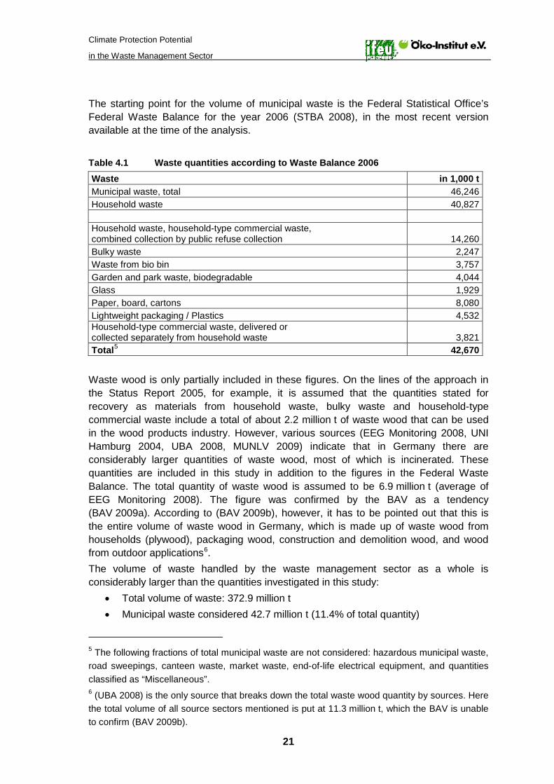
The starting point for the volume of municipal waste is the Federal Statistical Office’s Federal Waste Balance for the year 2006 (STBA 2008), in the most recent version available at the time of the analysis. Table 4.1 Waste quantities according to Waste Balance 2006 Waste in 1,000 t Municipal waste, total 46,246 Household waste 40,827 Household waste, household-type commercial waste, combined collection by public refuse collection 14,260 Bulky waste 2,247 Waste from bio bin 3,757 Garden and park waste, biodegradable 4,044 Glass 1,929 Paper, board, cartons 8,080 Lightweight packaging / Plastics 4,532 Household-type commercial waste, delivered or collected separately from household waste 3,821 Total5 42,670
Waste wood is only partially included in these figures. On the lines of the approach in the Status Report 2005, for example, it is assumed that the quantities stated for recovery as materials from household waste, bulky waste and household-type commercial waste include a total of about 2.2 million t of waste wood that can be used in the wood products industry. However, various sources (EEG Monitoring 2008, UNI Hamburg 2004, UBA 2008, MUNLV 2009) indicate that in Germany there are considerably larger quantities of waste wood, most of which is incinerated. These quantities are included in this study in addition to the figures in the Federal Waste Balance. The total quantity of waste wood is assumed to be 6.9 million t (average of EEG Monitoring 2008). The figure was confirmed by the BAV as a tendency (BAV 2009a). According to (BAV 2009b), however, it has to be pointed out that this is the entire volume of waste wood in Germany, which is made up of waste wood from households (plywood), packaging wood, construction and demolition wood, and wood from outdoor applications6
The volume of waste handled by the waste management sector as a whole is considerably larger than the quantities investigated in this study:
.
• Total volume of waste: 372.9 million t • Municipal waste considered 42.7 million t (11.4% of total quantity)
5 The following fractions of total municipal waste are not considered: hazardous municipal waste, road sweepings, canteen waste, market waste, end-of-life electrical equipment, and quantities classified as “Miscellaneous”. 6 (UBA 2008) is the only source that breaks down the total waste wood quantity by sources. Here the total volume of all source sectors mentioned is put at 11.3 million t, which the BAV is unable to confirm (BAV 2009b).

Climate Protection Potential
in the Waste Management Sector
22
• Waste wood volume 6.9 million t (1.9% of total quantity) Rather more than half the total volume for the waste management sector is due to construction and demolition waste, and there are also large amounts of production waste and commercial waste, plus mining rubble. The assumption described above – that the 2.2 million t of household and bulky waste recovered as material consists of waste wood – implies that roughly 70% is recovered as energy. This figure is lower than the assumption made by the BAV. The BAV members alone needed some 4.13 million t of waste wood in 2007, so the BAV assumes that at least 80% is recovered as energy (cf. Chapter 4.10). As regards the quantity of waste wood recovered as energy, this study furthermore assumes that about 83,000 t/a of waste wood originates from M(B) plants. This is based on a plausibility assumption regarding the destinations of the high-calorific fraction from M(B) plants (cf. Chapter 4.5). Table 4.2 shows the waste streams in the scenarios for investigation. The individual streams are reported as shown. In other words: the credits for recycling of metals recovered from the ashes are credited to waste incineration plants, and the credits for thermal recovery of the high-calorific fraction are similarly credited to M(B) plants. Accordingly it has to be borne in mind that the quantities stated in the row “WIP (direct)” only reflect the input sent directly to WIPs (household waste, household-type commercial waste, bulky waste). Considerable additional quantities from M(B) plants are also incinerated in WIPs (cf. Chapter 4.5), as are in particular sorting and treatment residues from recovery of lightweight packaging. The paper, board and cartons (PBC) fraction can be increased by about 1.2 million t in 2020 by collecting 50% of the paper quantities which in 2006 were still present in the 18.1 million t of residual waste (14.3 million t of household waste and 3.8 million t of household-type commercial waste). In the case of bio waste and green waste it is assumed that the additional 2.3 million t removed from residual waste in 2020 (50% of bio waste and green waste in residual waste 2006) breaks down into roughly two thirds bio waste and one third green waste. This means that in 2020 separate collection shows an increase of approx. 1.5 million t bio waste and about 0.8 million t green waste. The Witzenhausen Institute (2009) arrives at similar results for bio waste. As a result of the increased collection of lightweight packaging and especially its extension to include non-packaging items made of the same materials, 50% of the metals (0.32 million t), plastics (0.64 million t) and recyclable composites (0.37 million t) contained in residual waste in 2006 are covered. Here it is assumed that only 50% of the total composites present in residual waste are recoverable. Thus in 2020 an additional 1.3 million t are collected as a result of the recyclables bin. Furthermore, it is assumed that of the nearly 700,000 t of waste wood in residual waste and household-type commercial waste, an additional 50% can be collected separately in 2020 (cf. Table 4.7).

Climate Protection Potential
in the Waste Management Sector
23
Table 4.2 Waste streams and increases or decreases due to changes in waste streams
Increase/ 2006 Actual 2020 T 2020 A Reduction
2020 AT 2020 A from
2006 mill. t/a % mill. t/a % mill. t/a % mill. t/a %* Landfill 0.09 0.2 0 0.0 0 0.0 -0.09 -100.0 WIP 10.80 22.8 10.86 22.9 7.80 16.5 -3.00 -27.8 M(B) plants 7.24 15.3 7.28 15.4 5.23 11.0 -2.01 -27.8 MBT 3.19 6.7 3.21 6.8 2.01 4.2 -1.18 -36.9 MBS/MPS 1.79 3.8 1.80 3.8 1.79 3.8 0.00 0.0 MA 2.26 4.8 2.27 4.8 1.43 3.0 -0.83 -36.9 Bio waste 3.76 7.9 3.76 7.9 5.27 11.1 1.51 40.2 Bio waste, compost 2.59 5.5 2.59 5.5 1.05 2.2 -1.54 -59.3 Bio waste, fermentation 1.17 2.5 1.17 2.5 4.22 8.9 3.05 260.3 Green waste 4.04 8.5 4.04 8.5 4.80 10.1 0.76 18.8 Green waste, compost 4.04 8.5 4.04 8.5 3.00 6.3 -1.04 -25.7 Green waste, fermentation 0 0.0 0 0.0 0.90 1.9 0.90 100.0 Green waste, incineration 0 0.0 0 0.0 0.90 1.9 0.90 100.0 PBC 8.08 17.1 8.08 17.1 9.24 19.5 1.16 14.4 Glass 1.93 4.1 1.93 4.1 1.93 4.1 0.00 0.0 LWP 4.53 9.6 4.53 9.6 0 0.0 -4.53 -100.0 Recyclables incl. LWP 0 0.0 0 0.0 5.85 12.3 5.85 100.0 Waste wood 6.9 14.6 6.9 14.6 7.25 15.3 0.35 5.1 Thermal recycling 4.71 9.9 4.71 9.9 5.06 10.7 0.35 7.4 Material recycling 2.19 4.6 2.19 4.6 2.19 4.6 0.00 0.0 Total 47.38 100.0 47.38 100.0 47.38 100.0 0.00 0.0
* percentage increase or decrease. Not change in percentage points! ** The term “LWP” is also used for the extended lightweight packaging fraction that includes non-packaging waste of similar material and small electrical appliances in scenarios 2020 A and 2020 AT. This also applies to all other tables and figures. Discrepancies in the totals are due to rounding differences
The recyclable quantities of around 5 million t/a that are no longer present in residual waste because of the increase in separate collection in 2020 A and 2020 AT are deducted in equal parts on a weighted basis from WIP (approx. 3 million t/a) and M(B) plants (approx. 2 million t/a) , which corresponds to a decline of about 28% in each case. Within the M(B) plants there is a shift away from MBT and MT towards MBS and MPS. As a result, MBT and MT lose about 37% throughput, while the input into MBS/MPS shows a slight increase of 1%. Owing to the relative increase in MBS/MPS, the decline in the share of residual waste which reaches a WIP after treatment in the M(B) plants is less marked.

Climate Protection Potential
in the Waste Management Sector
24
MBT is reported as a mix of aerobic and anaerobic MBT. According to the survey by (IAA/INTECUS 2008), anaerobic MBTs account for about 32% of throughput. For the scenarios 2020 A and 2020 AT it is assumed, on the lines of the thinking for bio waste, that there is an increase in the share due to anaerobic MBT. The scenario 2020 T includes optimisation in the fields of gas yield and the efficiency of micro CHP plants (cf. Chapter 4.5). For the quantity of approx. 2.2 million t which is shown in the Federal Waste Balance for residual waste for recovery as material, there is no clear statement of what recovery paths are actually meant. The survey by the Federal Statistical Office confines itself to asking whether the process involved is a D or R process under Annex II A or B of the Closed-Substance Cycle and Waste Management Act (KrW-/AbfG). The further analysis of this does not go into detailed processes, but merely into whether the recovery is as material or energy. Recovery of waste wood constituents appears plausible. As in the Status Report 2005, these are assumed to be used in the wood products industry. The entire additional waste wood quantity of around 0.35 million t/a in 2020 A is assumed to be thermally recycled, while the quantity recovered as material in 2006 remains constant in 2020. Table 4.3 shows the waste quantities per head that result from the waste streams in Table 4.2. Table 4.3 Waste streams per head (for population of 82.4 million) and the increase /
decrease resulting from changes in waste streams
2006 Actual 2020 T 2020 A Increase/ Reduction
2020 AT 2020 A from 2006 kg/head*a % kg/head*a % kg/head*a % kg/head*a % Landfill 1.1 0.2 0.0 0.0 0.0 0.0 -1.1 -100.0 WIP 131.1 22.8 131.8 22.9 94.7 16.5 -36.4 -27.8 MBT/MBS/MT 87.9 15.3 88.3 15.4 63.5 11.0 -24.4 -27.8 Bio waste 45.6 7.9 45.6 7.9 64.0 11.1 18.3 40.2 Green waste 49.0 8.5 49.0 8.5 58.3 10.1 9.2 18.8 PBC 98.1 17.1 98.1 17.1 112.1 19.5 14.1 14.4 Glass 23.4 4.1 23.4 4.1 23.4 4.1 0.0 0.0 LWP 55.0 9.6 55.0 9.6 71.0 12.4 16.0 29.1 Waste wood 83.7 14.6 83.7 14.6 88.0 15.3 4.2 5.1 Total 574.9 100.0 574.9 100.0 574.9 100.0 0.0 0.0
Discrepancies in the totals are due to rounding differences
4.2 Composition of waste
The calculations for the individual treatment stages and the possible quantity changes in the scenarios are largely based on the data on the composition of residual waste and household-type commercial waste by individual waste fractions. Here there is a lack of reliable up-to-date data. A nationwide sorting analysis of household waste was performed in 1987. More recent sorting analyses have been performed for the whole of Bavaria, and otherwise on a sample basis in other parts of Germany. However, these

Climate Protection Potential
in the Waste Management Sector
25
figures are not necessarily representative of the whole of Germany, and in some cases they display substantial discrepancies from each other due to different methods of sampling and classification. In view of the lack of reliable current data, this study uses the same data that formed the basis for the Status Report 2005 following Kern (2001), in the interests of keeping the results comparable. For the purpose of comparison, the IAA/INTECUS data for 2006 from the UFO-Plan research project 2008 are also shown in Table 4.4 and Table 4.5, as are the data for 2004 from the EdDE study 2005 and the data from the Bavarian sorting analysis of 2003. Table 4.4 Average composition of residual waste from private households
Average waste composition:
EdDE
(2005) for 2004 IAA/INTECUS (2008) for 2006
BayLfU (2003)7
Kern (2001)
Organic material 38.3% 30.9% 22.5% 29.6% Middle fraction 14.2% Wood 2.1% 1.9% 1.2% 1.6% Textiles 4.3% 4.9% 3.7% 2.6% Minerals 5.9% 4.6% 2.8% Composites 3.3% 4.7% 7.0% 6.9% Pollutants 0.6% 0.6% 0.4% Substances n.o.s. 8.4% 10.6% 1.1% 9.0% Fine fraction < 8 mm 14.3% 14.7% 10.9% 14.0% Ferrous/NF metals 2.5% 2.7% 2.4% 3.8% PBC 9.0% 10.5% 7.7% 14.3% Glass 4.6% 4.9% 4.4% 6.9% Plastics 6.7% 9.2% 7.0% 5.8% Nappies 14.7% 5.5% Checksum 100% 100% 100% 100%
Discrepancies in the totals are due to rounding differences
7 In Bavaria, 17 sorting campaigns were carried out over a period of a 5 years. The sorting campaigns lasted a total of 36 weeks. The analysis covered approx. 113 t, or the residual waste of some 29,000 people.

Climate Protection Potential
in the Waste Management Sector
26
Table 4.5 Average composition of household-type commercial waste
Average waste composition:
IAA/INTECUS (2008) for 2006
Kern (2001)
Organic material 13.2% 8.3% Middle fraction Wood 6.3% 12.2% Textiles 3.0% 1.8% Minerals 4.8% Composites 8.6% 12.5% Pollutants - Substances n.o.s. 7.3% 25% Fine fraction < 8 mm 17.5% 14.7% Ferrous/NF metals 3.0% 2.6% PBC 17.1% 7.4% Glass 4.4% 3.8% Plastics 14.8% 11.7% Nappies 0% Checksum 100% 100% To determine the quantities of recyclables that can be skimmed off from residual waste, a mix of the composition of waste collected via the grey bin (14.3 million t/a) and household-type commercial waste (3.8 million t/a) was created after Kern (2001). The resulting absolute quantities for the year 2006 and the quantities skimmed off from these for 2020 as described above are listed in Table 4.78 Table 4.6. shows the percentage composition of the residual waste mix for 2006 and the scenario 2020 T, and the composition for the scenarios 2020 A and 2020 AT that results after the recyclables have been skimmed off by separate collection.
8 The difference between the quantity of the residual waste mix in Table 4.7 and the total of the quantities in Table 4.2 disposed of in M(B) plants, WIPs and as landfill is due to the bulky waste which is also disposed of there. Its slight influence on the composition is unknown and is disregarded.
Climate Protection Potential
in the Waste Management Sector
27
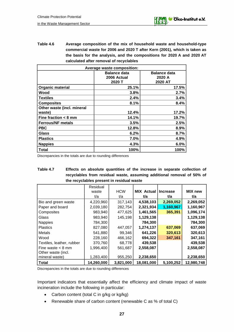
Table 4.6 Average composition of the mix of household waste and household-type commercial waste for 2006 and 2020 T after Kern (2001), which is taken as the basis for the analysis, and the compositions for 2020 A and 2020 AT calculated after removal of recyclables
Average waste composition:
Balance data 2006 Actual
2020 T
Balance data 2020 A
2020 AT Organic material 25.1% 17.5% Wood 3.8% 2.7% Textiles 2.4% 3.4% Composites 8.1% 8.4% Other waste (incl. mineral waste) 12.4% 17.2% Fine fraction < 8 mm 14.1% 19.7% Ferrous/NF metals 3.5% 2.5% PBC 12.8% 8.9% Glass 6.2% 8.7% Plastics 7.0% 4.9% Nappies 4.3% 6.0% Total 100% 100%
Discrepancies in the totals are due to rounding differences
Table 4.7 Effects on absolute quantities of the increase in separate collection of
recyclables from residual waste, assuming additional removal of 50% of the recyclables present in residual waste
Residual
waste HCW MIX Actual Increase MIX new t/a t/a t/a t/a t/a Bio and green waste 4,220,960 317,143 4,538,103 2,269,052 2,269,052 Paper and board 2,039,180 282,754 2,321,934 1,160,967 1,160,967 Composites 983,940 477,625 1,461,565 365,391 1,096,174 Glass 983,940 145,198 1,129,138 1,129,138 Nappies 784,300 784,300 784,300 Plastics 827,080 447,057 1,274,137 637,069 637,069 Metals 541,880 99,346 641,226 320,613 320,613 Wood 228,160 466,162 694,322 347,161 347,161 Textiles, leather, rubber 370,760 68,778 439,538 439,538 Fine waste < 8 mm 1,996,400 561,687 2,558,087 2,558,087 Other waste (incl. mineral waste) 1,283,400 955,250 2,238,650 2,238,650 Total 14,260,000 3,821,000 18,081,000 5,100,252 12,980,748
Discrepancies in the totals are due to rounding differences
Important indicators that essentially affect the efficiency and climate impact of waste incineration include the following in particular:
• Carbon content (total C in g/kg or kg/kg) • Renewable share of carbon content (renewable C as % of total C)

Climate Protection Potential
in the Waste Management Sector
28
• Fossil share of carbon content (fossil C as % of total C) • Calorific value (Hu in MJ/kg or kJ/kg)
In the case of the quantities of metal which are separated in M(B) plants or during treatment of ashes and which are capable of re-use, the content of ferrous and non-ferrous metals is also relevant. The indicators explained are listed in Table 4.9 for the relevant waste fractions. These are calculated on the basis of the composition of household waste and household-type commercial waste in 2006 and 2020 in conjunction with average indicators for the individual waste fractions. These indicators set out in Table 4.8 are averages obtained from the figures in various studies. As well as (IAA/INTECUS 2008), (Kern 2001) and (BayLfU 2003), these are (UBA Wien 2003), (AEA 2001), (IPCC 2006), (Ecoinvent 2007) and (ETC RWM 2008). Table 4.8 Calculated indicators for waste fractions
(Source: as stated in text, plus own calculations) C total C biogenic Cal. value Hu kg C/kg waste % of total C kJ/kg waste Bio and green waste 0.16 100% 4,620 Paper and board 0.37 100% 13,020 Composites 0.43 49% 18,017 Glass 0 0% 0 Nappies 0.18 75% 4,447 Plastics 0.68 0% 30,481 Metals 0 0% 0 Wood 0.38 100% 13,250 Textiles, leather, rubber 0.39 56% 15,020 Fine waste < 8mm 0.13 65% 5,133 Other waste (incl. mineral waste) 0.21 53% 7,800 Table 4.9 Key figures for important waste streams (Source: as stated in text, plus own calculations)
Unit Household
waste HCW Mix 2006 Mix 2020 A (HW) HW + HCW HW + HCW
Calorific value kJ/kg FS 8,508 11,757 9,195 8,478 C total g/kg FS 231 297 245 225 C renewable % Ctot 67 53 63 62 C fossil % Ctot 33 47 37 38 NF metals % solids 0.5 0.2 0.5 0.3 Iron and steel % solids 3.3 2.4 3.1 2.1 The metal contents in total residual waste as input into WIPS and M(B) plants are shown in Table 4.4 and Table 4.5 on the basis of the waste composition according to (Kern 2001). Ferrous and non-ferrous metals as shares of the total metals shown are derived on the basis of the ratio in the Status Report 2005.
Climate Protection Potential
in the Waste Management Sector
29
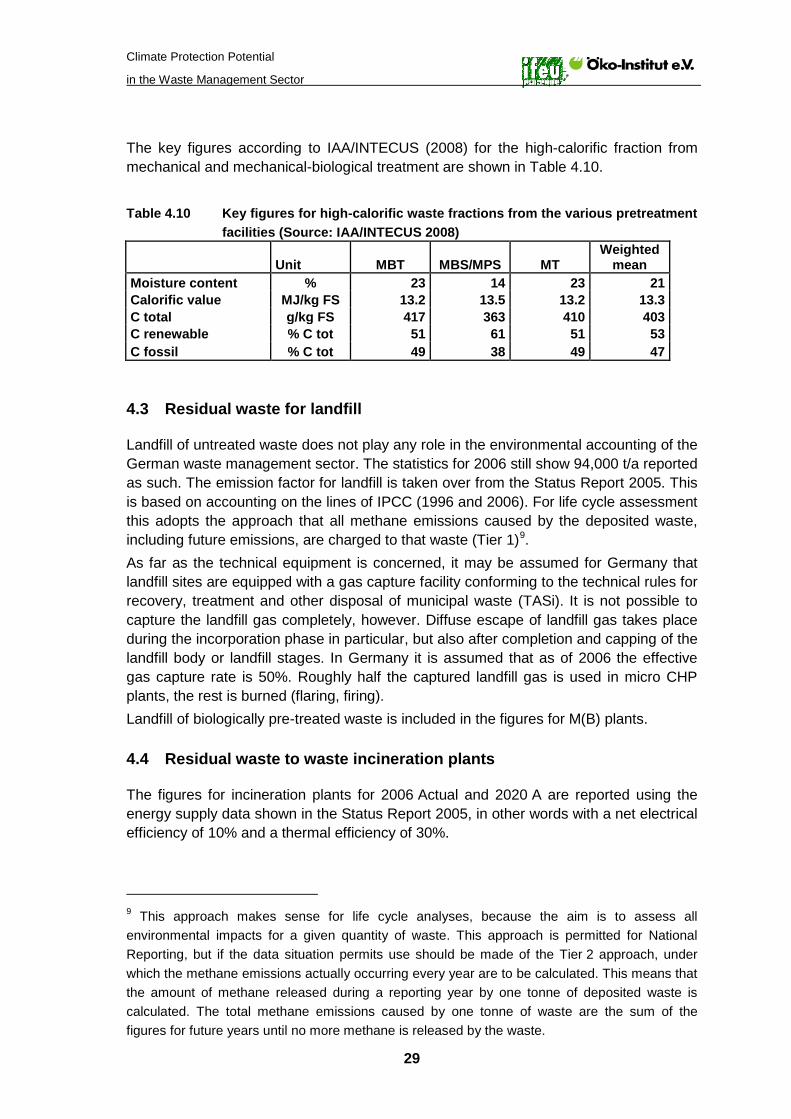
The key figures according to IAA/INTECUS (2008) for the high-calorific fraction from mechanical and mechanical-biological treatment are shown in Table 4.10. Table 4.10 Key figures for high-calorific waste fractions from the various pretreatment
facilities (Source: IAA/INTECUS 2008)
Unit MBT MBS/MPS MT Weighted
mean Moisture content % 23 14 23 21 Calorific value MJ/kg FS 13.2 13.5 13.2 13.3 C total g/kg FS 417 363 410 403 C renewable % C tot 51 61 51 53 C fossil % C tot 49 38 49 47
4.3 Residual waste for landfill
Landfill of untreated waste does not play any role in the environmental accounting of the German waste management sector. The statistics for 2006 still show 94,000 t/a reported as such. The emission factor for landfill is taken over from the Status Report 2005. This is based on accounting on the lines of IPCC (1996 and 2006). For life cycle assessment this adopts the approach that all methane emissions caused by the deposited waste, including future emissions, are charged to that waste (Tier 1)9
As far as the technical equipment is concerned, it may be assumed for Germany that landfill sites are equipped with a gas capture facility conforming to the technical rules for recovery, treatment and other disposal of municipal waste (TASi). It is not possible to capture the landfill gas completely, however. Diffuse escape of landfill gas takes place during the incorporation phase in particular, but also after completion and capping of the landfill body or landfill stages. In Germany it is assumed that as of 2006 the effective gas capture rate is 50%. Roughly half the captured landfill gas is used in micro CHP plants, the rest is burned (flaring, firing).
.
Landfill of biologically pre-treated waste is included in the figures for M(B) plants.
4.4 Residual waste to waste incineration plants
The figures for incineration plants for 2006 Actual and 2020 A are reported using the energy supply data shown in the Status Report 2005, in other words with a net electrical efficiency of 10% and a thermal efficiency of 30%.
9 This approach makes sense for life cycle analyses, because the aim is to assess all environmental impacts for a given quantity of waste. This approach is permitted for National Reporting, but if the data situation permits use should be made of the Tier 2 approach, under which the methane emissions actually occurring every year are to be calculated. This means that the amount of methane released during a reporting year by one tonne of deposited waste is calculated. The total methane emissions caused by one tonne of waste are the sum of the figures for future years until no more methane is released by the waste.

Climate Protection Potential
in the Waste Management Sector
30
For 2020 T and 2020 AT an improvement in net efficiency on the lines of (UBA 2007) is assumed for 2020: 14% electrical, 45% thermal. All electricity not needed to meet the plant’s internal requirements is fed into the grid. The relevant electricity credit is effected on the lines of the BMU method for determining the greenhouse gas saving due to electricity from renewable sources. The new expertise prepared for this purpose (ISI 2009) finds that of the electricity produced from biogenic waste in 2006, 16% replaced power from lignite, 59% power from coal, and 25% power from natural gas10. This is subject to a reduction factor of 852 g CO2/kWhel. However, this reduction factor takes account of direct CO2 emissions only, i.e. it does not include other greenhouse gases such as methane or laughing gas or the emissions due to providing the fuel supply. This study uses the above mentioned substitution mix according to (ISI 2009) consistently for all electricity generated in the waste management sector11
For the heat generated in the waste management system, credits are given for the substitution of oil and gas heating (50/50) in households. This too is largely in line with the BMU method as described in (BMU 2008), for example. New substitution potentials for heat from renewable energy sources are being worked out at the Federal Environment Agency (UBA), but were not yet available at the time of preparing this study. Losses of 10% are applied to distribution in district heating systems (cf. also Öko-Institut 2008c).
, but the relevant reduction factors are determined using own calculations, including prior chains and other greenhouse gases. In addition, the German electricity mix according to GEMIS is calculated for sensitivity purposes. Power requirements in incineration plants are met from their own electricity (GEMIS 1994 and 2008).
In 2006 and 2020 A, approx. 50% of the iron and 10% of the non-ferrous metals in the residual waste input into the incineration plants is separated from the ashes. The scenarios 2020 T and 2020 AT assume an improvement in metal separation to 70% for iron and 50% for non-ferrous metals (Öko-Institut 2002b). The change in waste composition resulting from the increase in separate collection is also accounted for in scenarios 2020 A and 2020 AT.
10 In 2007 the figure for electricity from gas was again 25%, but otherwise there was a marked change, with only 2% electricity from lignite and 73% from coal (reduction factor 820 g CO2/kWhel). The shift from lignite to coal was due to the unavailability of several nuclear power plants, which had to be made good by coal-fired power stations, and the lower price of CO2 allowances. 11 Regardless of the fact that under the BMU method electricity from different renewable energy sources is treated differently and that electricity from the fossil component of the waste is ignored. This uniform procedure has the advantage that the results are clearer and easier to analyse. It also serves the purpose in view, since this study is concerned with waste management issues and not, as in the BMU method, with the greenhouse gas savings potential of power generation from renewable energy sources.
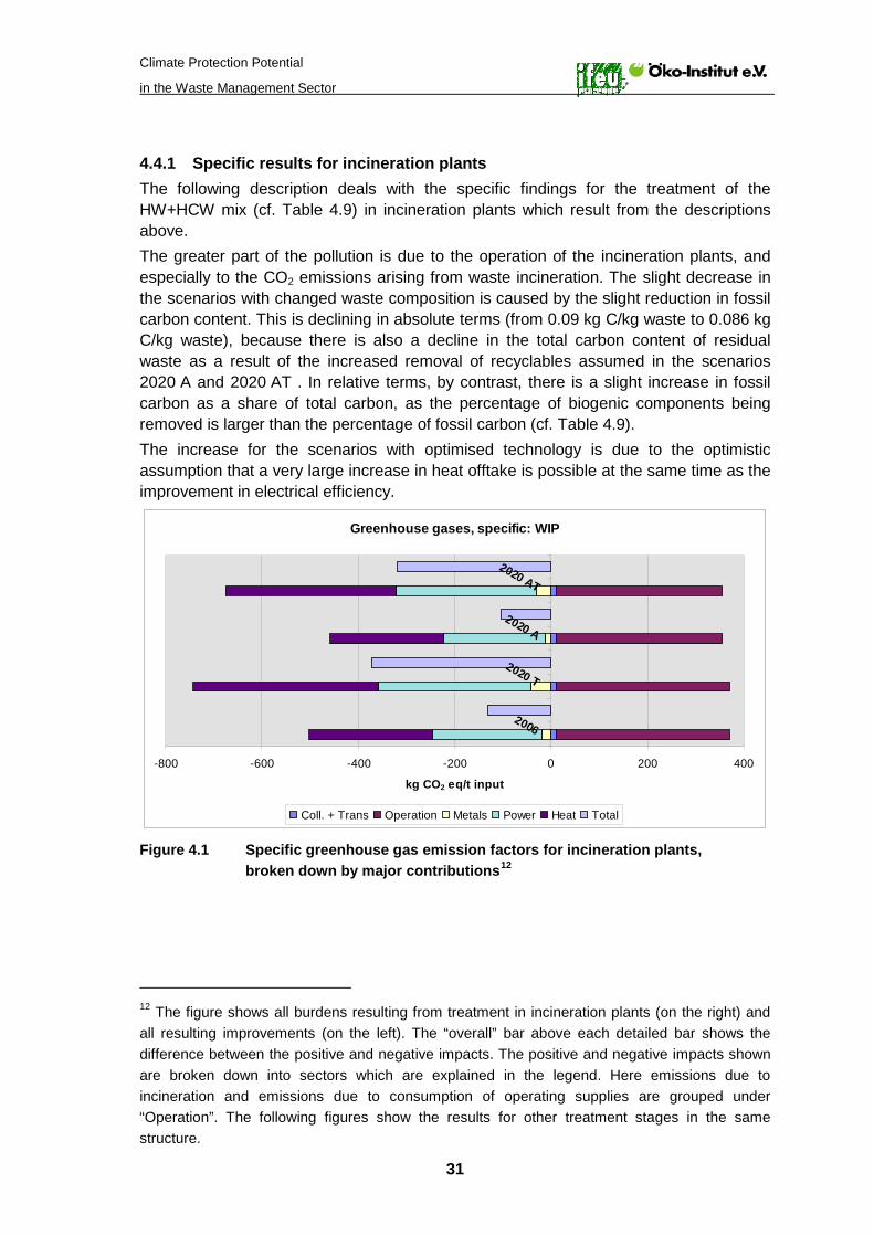
Climate Protection Potential
in the Waste Management Sector
31
4.4.1 Specific results for incineration plants The following description deals with the specific findings for the treatment of the HW+HCW mix (cf. Table 4.9) in incineration plants which result from the descriptions above. The greater part of the pollution is due to the operation of the incineration plants, and especially to the CO2 emissions arising from waste incineration. The slight decrease in the scenarios with changed waste composition is caused by the slight reduction in fossil carbon content. This is declining in absolute terms (from 0.09 kg C/kg waste to 0.086 kg C/kg waste), because there is also a decline in the total carbon content of residual waste as a result of the increased removal of recyclables assumed in the scenarios 2020 A and 2020 AT . In relative terms, by contrast, there is a slight increase in fossil carbon as a share of total carbon, as the percentage of biogenic components being removed is larger than the percentage of fossil carbon (cf. Table 4.9). The increase for the scenarios with optimised technology is due to the optimistic assumption that a very large increase in heat offtake is possible at the same time as the improvement in electrical efficiency.
Greenhouse gases, specific: WIP
-800 -600 -400 -200 0 200 400
2006
2020 T
2020 A
2020 AT
kg CO2 eq/t input
Coll. + Trans Operation Metals Power Heat Total
Figure 4.1 Specific greenhouse gas emission factors for incineration plants, broken down by major contributions12
12 The figure shows all burdens resulting from treatment in incineration plants (on the right) and all resulting improvements (on the left). The “overall” bar above each detailed bar shows the difference between the positive and negative impacts. The positive and negative impacts shown are broken down into sectors which are explained in the legend. Here emissions due to incineration and emissions due to consumption of operating supplies are grouped under “Operation”. The following figures show the results for other treatment stages in the same structure.

Climate Protection Potential
in the Waste Management Sector
32
Table 4.11 Specific greenhouse gas emission factors for incineration plants, broken down by major contributions
Greenhouse gases, specific kg CO2 eq/t
Components 2006 2020 T 2020 A 2020 AT Coll. +Trans. 9.5 9.5 9.4 9.5 Operation 361.5 361.5 346.1 346.1 Metals -18.9 -42.0 -13.2 -29.2 Electricity -226.5 -317.2 -208.9 -292.4 Heat -255.8 -383.6 -235.8 -353.7 EF WIP -130.2 -371.7 -102.3 -319.8
As expected, collection and transport (Coll. + Trans.) is not very important. Owing to the declining metal content of residual waste, the credits for recycling of metals show a considerable drop despite the assumption that they can be recovered with greater efficiency from grate ash. Recycling of waste incineration ash in road construction can offset the cost of processing, and thus accounts for a small share of the credits for metal recycling.
4.4.2 Specific results of sensitivity analyses for incineration plants A number of sensitivity analyses (cf. Chapter 6) were made to investigate the influence of various factors on the results of the balance. The following have a particularly large influence on the contributions made by incineration plants:
• electricity supplied is not credited to the fossil electricity mix according to (ISI 2009), but to the electricity mix for Germany (Sens 2: E mix, see also Chapter 6.2)
• the share of renewable carbon is adjusted upwards (Sens 3: C reg high (10% higher than standard)) and
• the share of renewable carbon is adjusted downwards (Sens 4: C reg low (13% lower than standard)) (see also Chapter 6.3.1)
• for scenarios 2020 T and 2020 AT the efficiency of the incineration plants is reduced to the standard assumed for the 2020 scenarios in the Status Report 2005: power 15%, heat 36.8% (Sens 5: eta Status Report)
Figure 4.2 and Table 4.12 show the effect of these sensitivity analyses on the specific emission factors for incineration plants in the scenario 2020 AT.
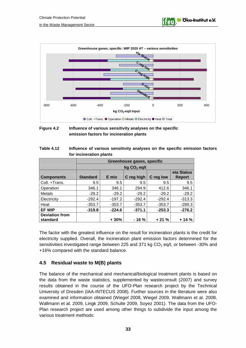
Climate Protection Potential
in the Waste Management Sector
33
Greenhouse gases, specific: WIP 2020 AT – various sensitivities
-800 -600 -400 -200 0 200 400
Standard
E mix
C reg high
C reg low
eta Status
kg CO2-eq/t input
Coll. +Trans. Operation Metals Electricity Heat Total
Figure 4.2 Influence of various sensitivity analyses on the specific emission factors for incineration plants
Table 4.12 Influence of various sensitivity analyses on the specific emission factors
for incineration plants
Greenhouse gases, specific
kg CO2 eq/t
Components Standard E mix C reg high C reg low eta Status
Report Coll. +Trans. 9.5 9.5 9.5 9.5 9.5 Operation 346.1 346.1 294.9 412.6 346.1 Metals -29.2 -29.2 -29.2 -29.2 -29.2 Electricity -292.4 -197.2 -292.4 -292.4 -313.3 Heat -353.7 -353.7 -353.7 -353.7 -289.3 EF WIP -319.8 -224.6 -371.1 -253.3 -276.2 Deviation from standard + 30% - 16 % + 21 % + 14 %
The factor with the greatest influence on the result for incineration plants is the credit for electricity supplied. Overall, the incineration plant emission factors determined for the sensitivities investigated range between 225 and 371 kg CO2 eq/t, or between -30% and +16% compared with the standard balance.
4.5 Residual waste to M(B) plants
The balance of the mechanical and mechanical/biological treatment plants is based on the data from the waste statistics, supplemented by wasteconsult (2007) and survey results obtained in the course of the UFO-Plan research project by the Technical University of Dresden (IAA-INTECUS 2008). Further sources in the literature were also examined and information obtained (Wiegel 2008, Wiegel 2009, Wallmann et al. 2008, Wallmann et al. 2009, Lingk 2009, Schulte 2009, Soyez 2001). The data from the UFO-Plan research project are used among other things to subdivide the input among the various treatment methods:
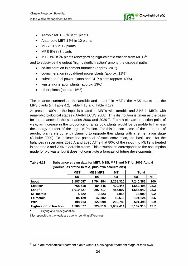
Climate Protection Potential
in the Waste Management Sector
34
• Aerobic MBT 30% in 21 plants • Anaerobic MBT 14% in 10 plants • MBS 19% in 12 plants • MPS 6% in 3 plants • MT 31% in 26 plants (disregarding high-calorific fraction from MBT)13
and to subdivide the output “high-calorific fraction” among the disposal paths
• co-incineration in cement furnaces (approx. 20%) • co-incineration in coal-fired power plants (approx. 11%) • substitute-fuel power plants and CHP plants (approx. 40%) • waste incineration plants (approx. 13%) • other plants (approx. 16%)
The balance summarises the aerobic and anaerobic MBTs, the MBS plants and the MPS plants (cf. Table 4.2, Table 4.13 and Table 4.17). At present, 69% of the input is treated in MBTs with aerobic and 31% in MBTs with anaerobic biological stages (IAA-INTECUS 2008). This distribution is taken as the basis for the balances in the scenarios 2006 and 2020 T. From a climate protection point of view, an increase in the proportion of anaerobic plants would be desirable to harness the energy content of the organic fraction. For this reason some of the operators of aerobic plants are currently planning to upgrade their plants with a fermentation stage (Schulte 2009). To indicate the potential of such conversion, the basis used for the balances in scenarios 2020 A and 2020 AT is that 80% of the input into MBTs is treated in anaerobic and 20% in aerobic plants. This assumption corresponds to the assumption made for bio waste, but it does not constitute a forecast of future developments. Table 4.13 Substance stream data for MBT, MBS, MPS and MT for 2006 Actual (Source: as stated in text, plus own calculations) MBT MBS/MPS MT Total t/a t/a t/a t/a % Input 3,187,087 1,794,984 2,258,310 7,240,381 100 Losses* 768,618 484,345 429,445 1,682,408 23.2 Landfill 1,019,327 207,717 457,997 1,685,042 23.3 NF metals 5,722 3,223 4,055 13,000 0.2 Fe metals 84,129 47,382 59,613 191,124 2.6 WIP 108,713 122,998 269,786 501,498 6.9 High-calorific fraction 1,200,577 929,319 1,037,414 3,167,310 43.7
* Drying and biodegradation Discrepancies in the totals are due to rounding differences
13 MTs are mechanical treatment plants without a biological treatment stage of their own
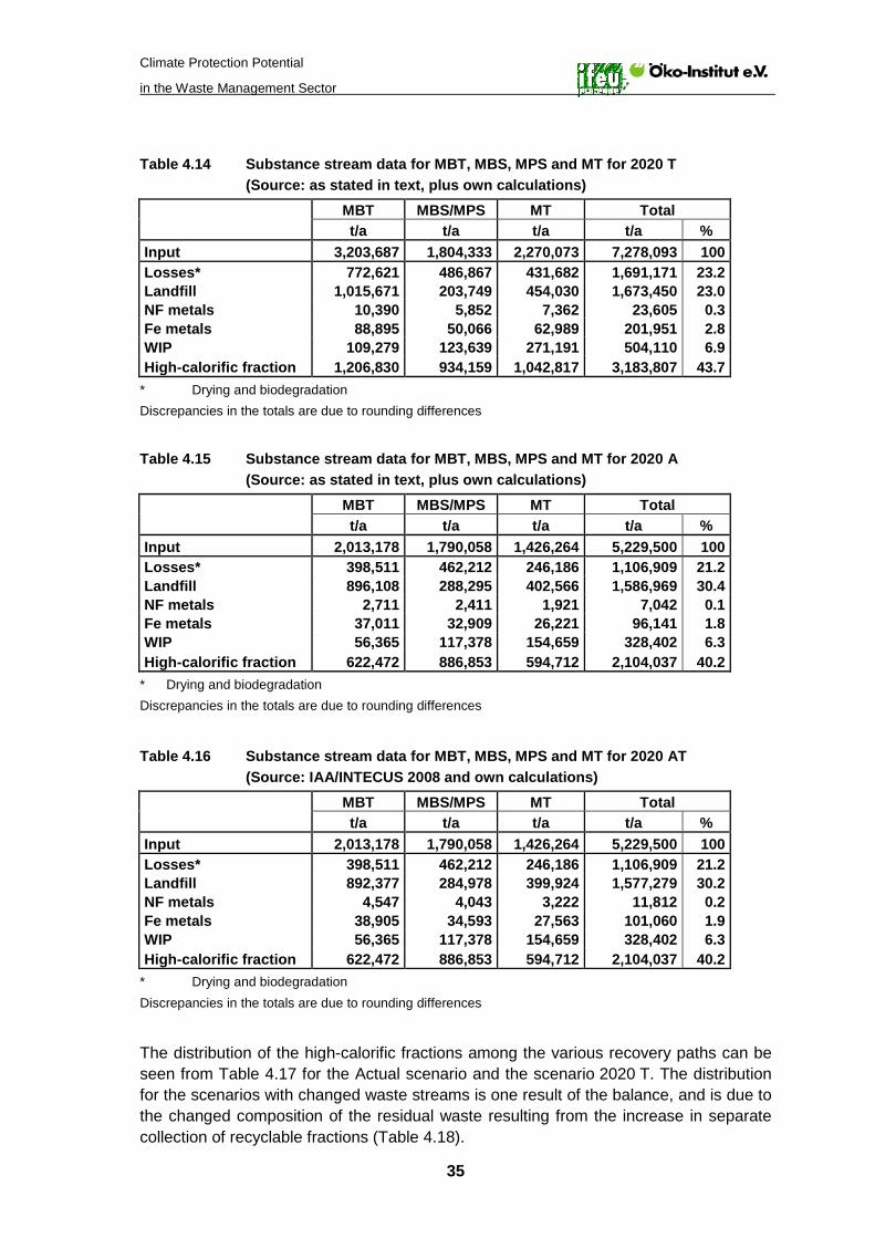
Climate Protection Potential
in the Waste Management Sector
35
Table 4.14 Substance stream data for MBT, MBS, MPS and MT for 2020 T (Source: as stated in text, plus own calculations) MBT MBS/MPS MT Total t/a t/a t/a t/a % Input 3,203,687 1,804,333 2,270,073 7,278,093 100 Losses* 772,621 486,867 431,682 1,691,171 23.2 Landfill 1,015,671 203,749 454,030 1,673,450 23.0 NF metals 10,390 5,852 7,362 23,605 0.3 Fe metals 88,895 50,066 62,989 201,951 2.8 WIP 109,279 123,639 271,191 504,110 6.9 High-calorific fraction 1,206,830 934,159 1,042,817 3,183,807 43.7
* Drying and biodegradation Discrepancies in the totals are due to rounding differences
Table 4.15 Substance stream data for MBT, MBS, MPS and MT for 2020 A (Source: as stated in text, plus own calculations) MBT MBS/MPS MT Total t/a t/a t/a t/a % Input 2,013,178 1,790,058 1,426,264 5,229,500 100 Losses* 398,511 462,212 246,186 1,106,909 21.2 Landfill 896,108 288,295 402,566 1,586,969 30.4 NF metals 2,711 2,411 1,921 7,042 0.1 Fe metals 37,011 32,909 26,221 96,141 1.8 WIP 56,365 117,378 154,659 328,402 6.3 High-calorific fraction 622,472 886,853 594,712 2,104,037 40.2
* Drying and biodegradation Discrepancies in the totals are due to rounding differences
Table 4.16 Substance stream data for MBT, MBS, MPS and MT for 2020 AT (Source: IAA/INTECUS 2008 and own calculations) MBT MBS/MPS MT Total t/a t/a t/a t/a % Input 2,013,178 1,790,058 1,426,264 5,229,500 100 Losses* 398,511 462,212 246,186 1,106,909 21.2 Landfill 892,377 284,978 399,924 1,577,279 30.2 NF metals 4,547 4,043 3,222 11,812 0.2 Fe metals 38,905 34,593 27,563 101,060 1.9 WIP 56,365 117,378 154,659 328,402 6.3 High-calorific fraction 622,472 886,853 594,712 2,104,037 40.2
* Drying and biodegradation Discrepancies in the totals are due to rounding differences
The distribution of the high-calorific fractions among the various recovery paths can be seen from Table 4.17 for the Actual scenario and the scenario 2020 T. The distribution for the scenarios with changed waste streams is one result of the balance, and is due to the changed composition of the residual waste resulting from the increase in separate collection of recyclable fractions (Table 4.18).
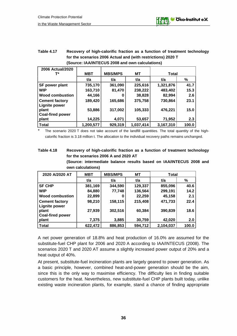
Climate Protection Potential
in the Waste Management Sector
36
Table 4.17 Recovery of high-calorific fraction as a function of treatment technology
for the scenarios 2006 Actual and (with restrictions) 2020 T (Source: IAA/INTECUS 2008 and own calculations)
2006 Actual/2020 T* MBT MBS/MPS MT Total
t/a t/a t/a t/a % SF power plant 735,170 361,090 225,616 1,321,876 41.7 WIP 163,710 81,470 238,222 483,402 15.3 Wood combustion 44,166 0 38,828 82,994 2.6 Cement factory 189,420 165,686 375,758 730,864 23.1 Lignite power plant 53,886 317,002 105,333 476,221 15.0 Coal-fired power plant 14,225 4,071 53,657 71,952 2.3 Total 1,200,577 929,319 1,037,414 3,167,310 100.0 * The scenario 2020 T does not take account of the landfill quantities. The total quantity of the high-
calorific fraction is 3.18 million t. The allocation to the individual recovery paths remains unchanged.
Table 4.18 Recovery of high-calorific fraction as a function of treatment technology
for the scenarios 2006 A and 2020 AT (Source: intermediate balance results based on IAA/INTECUS 2008 and
own calculations)
2020 A/2020 AT MBT MBS/MPS MT Total t/a t/a t/a t/a % SF CHP 381,169 344,590 129,337 855,096 40.6 WIP 84,880 77,748 136,564 299,191 14.2 Wood combustion 22,899 0 22,259 45,158 2.1 Cement factory 98,210 158,115 215,408 471,733 22.4 Lignite power plant 27,939 302,516 60,384 390,839 18.6 Coal-fired power plant 7,375 3,885 30,759 42,020 2.0 Total 622,472 886,853 594,712 2,104,037 100.0 A net power generation of 18.8% and heat production of 16.0% are assumed for the substitute-fuel CHP plant for 2006 and 2020 A according to IAA/INTECUS (2008). The scenarios 2020 T and 2020 AT assume a slightly increased power output of 20% and a heat output of 40%. At present, substitute-fuel incineration plants are largely geared to power generation. As a basic principle, however, combined heat-and-power generation should be the aim, since this is the only way to maximise efficiency. The difficulty lies in finding suitable customers for the heat. Nevertheless, new substitute-fuel CHP plants built today, unlike existing waste incineration plants, for example, stand a chance of finding appropriate
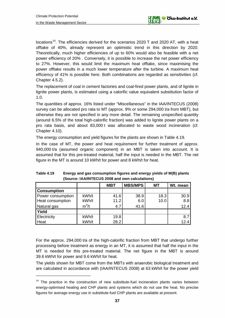
Climate Protection Potential
in the Waste Management Sector
37
locations14
4.5.2
. The efficiencies derived for the scenarios 2020 T and 2020 AT, with a heat offtake of 40%, already represent an optimistic trend in this direction by 2020. Theoretically, much higher efficiencies of up to 60% would also be feasible with a net power efficiency of 20% . Conversely, it is possible to increase the net power efficiency to 27%. However, this would limit the maximum heat offtake, since maximising the power offtake results in a much lower temperature after the turbine. A maximum heat efficiency of 41% is possible here. Both combinations are regarded as sensitivities (cf. Chapter ). The replacement of coal in cement factories and coal-fired power plants, and of lignite in lignite power plants, is estimated using a calorific value equivalent substitution factor of 1.0. The quantities of approx. 16% listed under “Miscellaneous” in the IAA/INTECUS (2008) survey can be allocated pro rata to MT (approx. 9% or some 294,000 t/a from MBT), but otherwise they are not specified in any more detail. The remaining unspecified quantity (around 6.5% of the total high-calorific fraction) was added to lignite power plants on a pro rata basis, and about 83,000 t was allocated to waste wood incineration (cf. Chapter 4.10). The energy consumption and yield figures for the plants are shown in Table 4.19. In the case of MT, the power and heat requirement for further treatment of approx. 940,000 t/a (assumed organic component) in an MBT is taken into account. It is assumed that for this pre-treated material, half the input is needed in the MBT. The net figure in the MT is around 10 kWh/t for power and 8 kWh/t for heat. Table 4.19 Energy and gas consumption figures and energy yields of M(B) plants (Source: IAA/INTECUS 2008 and own calculations)
MBT MBS/MPS MT Wt. mean Consumption Power consumption kWh/t 41.6 38.9 18.3 30.9 Heat consumption kWh/t 11.2 6.0 10.0 8.8 Natural gas m3/t 4.7 41.6 12.4 Yield Electricity kWh/t 19.8 8.7 Heat kWh/t 28.2 12.4 For the approx. 294,000 t/a of the high-calorific fraction from MBT that undergo further processing before treatment as energy in an MT, it is assumed that half the input in the MT is needed for this pre-treated material. The net figure in the MBT is around 39.6 kWh/t for power and 9.6 kWh/t for heat. The yields shown for MBT come from the MBTs with anaerobic biological treatment and are calculated in accordance with (IAA/INTECUS 2008) at 63 kWh/t for the power yield
14 The practice in the construction of new substitute-fuel incineration plants varies between energy-optimised heating and CHP plants and systems which do not use the heat. No precise figures for average energy use in substitute-fuel CHP plants are available at present.

Climate Protection Potential
in the Waste Management Sector
38
and 90 kWh/t for the heat yield. The associated biogas yield works out at 38 m³/t waste. These results are based on the figures for three plants. The data obtained were compared with figures according to (Wallmann et al. 2008), which are based on reports from five anaerobic MBTs. The resulting power yield for biogas recovery is 99 kWh/t, and the heat yield is 115 kWh/t for a mean gas yield of 45 Nm³/t waste normalised to a methane content of 60 vol%. In (Wallmann et al. 2008) this gas yield is regarded as low, since this average value also takes account of two split-stream fermentation plants which have relatively low gas yields of 9 and 26 Nm³/t waste respectively. For the three full-stream fermentation plants, by contrast, gas yields of between 60 and 65 Nm³/t waste were calculated. It is also reported in (Wallmann et al. 2008) that pilot-scale and large-scale tests revealed gas yields of between 60 and 90 Nm³/t waste with a methane content of 64 vol%, and that figures of up to 100 Nm³/t waste were possible as a result of further optimisation measures. The findings of (IAA/INTECUS 2008) and (Wallmann et al. 2008) show that there are considerable differences between the individual plants with regard to their energy balance. For the purpose of balances for the M(B) plants, (IAA/INTECUS 2008) was used as the sole source for the scenario 2006, and hence also the above mentioned heat and power yields for the anaerobic MBTs. Figures based on (Wallmann et al. 2008) are derived to take account of technical optimisation potential in the scenarios 2020 T and 2020 AT. The gas yield is taken as 75 Nm³/t waste, with a methane content of 60 vol%. The efficiency figures for micro CHP plants are calculated as 37% for power and 43% for heat. This results in a power yield of around 166 kWh/t and a heat yield of around 193 kWh/t. As for a waste incineration plant, the energy generated was reduced by deducting internal power requirements, which were again calculated in accordance with (Wallmann et al. 2008). Of the remaining excess energy, the power is credited in full, while in the case of heat it is assumed, on the lines of the procedure in bio waste fermentation in scenario 2006 Actual, that 20% can be used externally. For the scenario 2020 T an increase to 80% utilisation of the excess heat is assumed. The assumptions described above for the scenarios for residual waste treatment in M(B) plants are summed up again in Table 4.20.
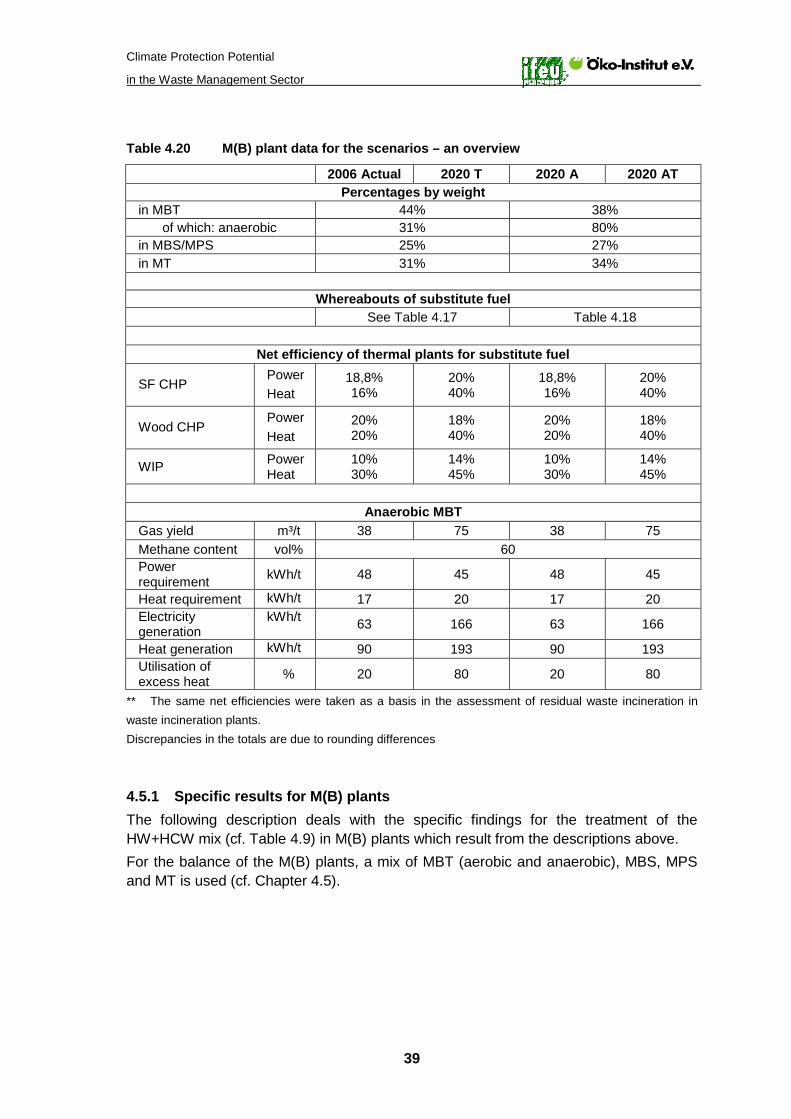
Climate Protection Potential
in the Waste Management Sector
39
Table 4.20 M(B) plant data for the scenarios – an overview
2006 Actual 2020 T 2020 A 2020 AT Percentages by weight
in MBT 44% 38% of which: anaerobic 31% 80%
in MBS/MPS 25% 27% in MT 31% 34%
Whereabouts of substitute fuel
See Table 4.17 Table 4.18
Net efficiency of thermal plants for substitute fuel
SF CHP Power Heat
18,8% 16%
20% 40%
18,8% 16%
20% 40%
Wood CHP Power Heat
20% 20%
18% 40%
20% 20%
18% 40%
WIP Power Heat
10% 30%
14% 45%
10% 30%
14% 45%
Anaerobic MBT
Gas yield m³/t 38 75 38 75 Methane content vol% 60 Power requirement kWh/t 48 45 48 45
Heat requirement kWh/t 17 20 17 20 Electricity generation
kWh/t 63 166 63 166
Heat generation kWh/t 90 193 90 193 Utilisation of excess heat % 20 80 20 80
** The same net efficiencies were taken as a basis in the assessment of residual waste incineration in waste incineration plants. Discrepancies in the totals are due to rounding differences
4.5.1 Specific results for M(B) plants The following description deals with the specific findings for the treatment of the HW+HCW mix (cf. Table 4.9) in M(B) plants which result from the descriptions above. For the balance of the M(B) plants, a mix of MBT (aerobic and anaerobic), MBS, MPS and MT is used (cf. Chapter 4.5).

Climate Protection Potential
in the Waste Management Sector
40
Greenhouse gases, specific: M(B) plants
-350 -300 -250 -200 -150 -100 -50 0 50 100
2006
2020 T
2020 A
2020 AT
kg CO2-eq/t input
Coll. + Trans Operation Power & Heat Landfill Metals WIP High-cal. Total
Figure 4.3 Specific greenhouse gas emission factors for M(B) plants, broken down by major contributions
Table 4.21 Specific greenhouse gas emission factors for M(B) plants, broken down by
major contributions Greenhouse gases, specific kg CO2 eq/t
Components 2006 2020 T 2020 A 2020 AT Coll. +Trans. 17.2 17.3 16.5 16.6 Operation 28.4 28.6 25.4 25.4 Power & Heat -2.5 -21.2 -5.6 -47.3 Landfill 3.4 3.4 4.5 4.4 Metals -41.7 -56.4 -29.0 -39.3 WIP -6.4 -42.6 -3.5 -34.3 High-calorific -136.6 -199.9 -130.0 -186.4 EF M(B) plants -138.1 -270.8 -121.7 -260.8
Collection, transport and landfill deposition represent a very constant burden. Operating expenses are down in the scenarios 2020 A and 2020 AT as a result of redirection from aerobic to anaerobic within the MBT, which means that considerably less external energy needs to be purchased. The result is dominated by the use of the high-calorific fractions. In the scenarios 2006 Actual and 2020 T, another major factor is the recycling of the metals. In scenarios 2020 A and 2020 AT the contribution by metals is lower, as the metal concentrations in the residual waste are also lower. The incineration component is increased by the efficiency improvements in waste incineration plants. This applies similarly to the share of power and heat achieved as a result of the improvement in efficiency (gas yield, micro CHP efficiency) in anaerobic MBTs.
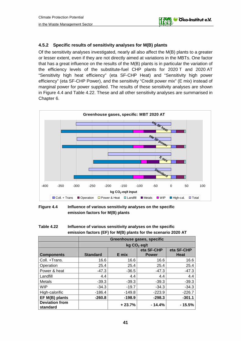
Climate Protection Potential
in the Waste Management Sector
41
4.5.2 Specific results of sensitivity analyses for M(B) plants Of the sensitivity analyses investigated, nearly all also affect the M(B) plants to a greater or lesser extent, even if they are not directly aimed at variations in the MBTs. One factor that has a great influence on the results of the M(B) plants is in particular the variation of the efficiency levels of the substitute-fuel CHP plants for 2020 T and 2020 AT “Sensitivity high heat efficiency” (eta SF-CHP Heat) and “Sensitivity high power efficiency” (eta SF-CHP Power), and the sensitivity “Credit power mix” (E mix) instead of marginal power for power supplied. The results of these sensitivity analyses are shown in Figure 4.4 and Table 4.22. These and all other sensitivity analyses are summarised in Chapter 6.
Greenhouse gases, specific: MBT 2020 AT
-400 -350 -300 -250 -200 -150 -100 -50 0 50 100
Standard
E mix
eta SF power
eta SF heat
kg CO2-eq/t input
Coll. + Trans Operation Power & Heat Landfill Metals WIP High-cal. Total
Figure 4.4 Influence of various sensitivity analyses on the specific emission factors for M(B) plants
Table 4.22 Influence of various sensitivity analyses on the specific
emission factors (EF) for M(B) plants for the scenario 2020 AT Greenhouse gases, specific kg CO2 eq/t
Components Standard E mix eta SF-CHP
Power eta SF-CHP
Heat Coll. +Trans. 16.6 16.6 16.6 16.6 Operation 25.4 25.4 25.4 25.4 Power & heat -47.3 -36.5 -47.3 -47.3 Landfill 4.4 4.4 4.4 4.4 Metals -39.3 -39.3 -39.3 -39.3 WIP -34.3 -19.7 -34.3 -34.3 High-calorific -186.4 -149.8 -223.9 -226.7 EF M(B) plants -260.8 -198.9 -298.3 -301.1 Deviation from standard + 23.7% - 14.4% - 15.5%

Climate Protection Potential
in the Waste Management Sector
42
Compared with the standard case, the sensitivity analysis “E mix” has the greatest influence on the results for the M(B) plants (+24%). If, instead of marginal power, the average power mix is credited for electricity supplied, the net relief achieved is much lower because the power mix also includes electricity from renewable energy sources and nuclear power, which involve little or no emission of greenhouse gases. Higher average efficiency levels of the substitute-fuel power plants result in an increase of around 15% in greenhouse gas savings, regardless of whether the main focus of the increase is power efficiency or heat efficiency. Since M(B) plants also supply fractions to waste incineration plants, the sensitivities for waste incineration plants “Sensitivity high/low carbon content” (C reg high, C reg low) and “Sensitivity efficiencies waste incineration plants” (eta Status Report) have a certain influence on the balance for the M(B) plants (cf. Chapters 4.4.2 and Table 4.12). However, the resulting reductions or increases in the emission factor of the M(B) plants do not exceed about 4%.
4.6 Bio and green waste
At present, bio waste and green waste15
According to (FZKA 2003) the capacity merely for fermentation of bio waste was determined from a survey of the federal states as 821,000 t/a, which corresponds to about 22% of the bio waste volume for 2006. However, it is not possible to provide any information on utilisation levels. (IE/IZES 2006) also cites anaerobic treatment capacities, but these only come to around 420,000 t/a. These figures are further subdivided into about 350,000 t/a for bio waste and 70,000 t/a for green waste.
are largely composted. In (Witzenhausen-Institut 2008), the capacity of fermentation plants accounts for about 15% of the total capacity of about 13 million t/a quoted for bio and green waste. In terms of the quantity of bio waste from households, this would be about 30%. However, the study does not provide any information on utilisation levels or the share of bio waste from households. According to reports by RETERRA (2009), only about 10% of bio waste from its corporate association is sent for fermentation.
A recently published analysis by the Federal Composting Association (BGK 2009) indicates that in the currently 88 biogas plants subject to quality assurance, with a total input quantity of 2.3 million t/a. a share of 17% comes from bio bins. Recalculated in terms of the bio waste quantity from households in 2006, this corresponds to 10%. The sources mentioned suggest a range of between 10 and 30% for the possible share of bio waste fermented. The balance for the scenario 2006 Actual uses the mean of 15%. For 2020 A and 2020 AT it is assumed that composting units are upgraded by adding a fermentation stage in order to achieve the combined energy and materials recovery which makes sense from a climate protection point of view (Öko-Institut 2004, IFEU/Öko-Institut 2006). According to (Witzenhausen-Institut/igw Witzenhausen 2007), suitable candidates for upgrading are technically advanced systems with a minimum size of 10,000 t/a. This corresponds to a potential of 220-250 plants or an annual 15 In the context of the balance, the distinction between bio waste and green waste is defined as follows: bio waste is the contents of the bio bin, while the remainder is referred to as green waste.

Climate Protection Potential
in the Waste Management Sector
43
capacity of around 7 million t/a. For the 5.27 million t of bio waste (Chapter 4.1) resulting from increased separate collection in 2020, it is assumed that 80% will be fermented in upgraded plants and 20% will continue to go to existing composting units. In combination with the green waste also sent for fermentation in the scenario 2020 A (see below), there will then be a total of 5.1 million t/a for fermentation. In the scenarios 2020 A and 2020 AT, a separation of substance streams (50% composting, 25% fermentation, 25% combustion) is entered in the balance for 75% of the volume of green waste. According to (EdDE 2007) it is possible to separate 25-30% wood waste with a calorific value of up to 15 MJ/kg by means of suitable grading and drying. The calculations use a conservative calorific value of 9.36 MJ/kg for black wood chips (IFEU/igw Witzenhausen 2008). Combustion of the woody green waste takes place in energy-efficient biomass or wood incineration plants. The efficiencies that can be achieved are the same as those used for incineration of waste wood (cf. Chapter 4.10). Also according to (EdDE 2007), 15-30% of green waste is suitable for fermentation. The herbaceous green waste which accounts for 19% of total green waste and which is allocated to fermentation in the scenarios 2020 A and 2020 AT, is assumed to be mixed and jointly treated in fermentation plants. For the gas yield from this mixture, it is assumed that the slightly lower gas potential is cancelled out by technical improvements in the fermentation plants and that, as with fermentation of bio waste in 2006 Actual, 100 m3 of biogas is obtained per tonne of bio and green waste mixture.
4.6.1 Composting No statistical data are available on the technical facilities of composting plants. According to the requirements of the Technical Instructions for Air Quality Control (TA Luft 2002), plants with an annual throughput of over 10,000 t/a are now to be designed on a closed basis. In practice this is not always the case. However, it may largely be assumed that plants with an annual throughput in excess of 20,000 t/a are run on a closed basis. In terms of treatment capacity this is equivalent to 5.4 million t/a, or 56% of the total capacity investigated as of 2003 according to (Witzenhausen-Institut/igw Witzenhausen 2007) (Table 4.23)16
According to (BGK 2004), of the 431 member plants with a treatment capacity of around 7 million t/a some 290 plants or about 67% were of open design
.
17
16 This survey analysed 668 of the 813 plants which existed at the time according to BGK (
. Approximately 70% of these plants have a capacity in excess of 10,000 t/a. Applied to the figures in (Witzenhausen-Institut/igw Witzenhausen 2007), the 67% open plants would account for only 27% of the total treatment capacity, in other words approximately 2.6 million t/a would be treated in open plants and about 7 million t/a in closed ones. In 2008 some 534 plants with a capacity of around 8 million t/a were members of the BGK (H&K aktuell 3/2009), and for these the analyses according to (BGK 2004) should still be transferable. This would mean that the above mentioned assumption that only plants
www.bgk.de; status 2006). It is assumed that the 145 remaining plants with a capacity of around 0.45 million t/a are mostly small green waste composting plants. 17 123 straight green waste composting plants, 167 plants handling bio and green waste. Of the latter, 67 were in the New Länder.

Climate Protection Potential
in the Waste Management Sector
44
with a capacity in excess of 20,000 t/a were of closed design was an under-estimate. According to (Burth 2009), however, there are – especially in the New Länder – large plants which do not belong to the BGK and which perform open composting in clamps. According to an overview of plants in Saxony-Anhalt for 2004, there were about 125 composting plants with a total capacity of over 1 million t/a. Of these, however, only 9 plants with open clamp composting have a throughput capacity in excess of 20,000 t/a, and these are used to treat not only bio and green waste, but also other waste such as sewage sludge. According to (IE/IZES 2006), the federal states of Thuringia, Saxony-Anhalt, Saxony and Brandenburg have a total aerobic and anaerobic treatment capacity about 1 to 1.5 million t/a in each case, but the throughput capacity for bio and green waste is only around 150,000 to 200,000 t/a per state. According to the Federal Environment Agency18, green waste is almost entirely treated in open plants, which agrees with the information supplied by (BGK 2004)19
. Since green waste is also treated jointly with bio waste, it is assumed for 2006 that 90% of the total green waste quantity was treated in open plants. This corresponds to 3.6 million t/a, which is well above the figure of 2.6 million t/a found by (BGK 2004). Conversely, it is assumed for bio waste that this is largely treated in closed plants and only 10% in open plants. Overall, this results in a total of nearly 4 million t/a treated in open plants, which is regarded as average for Germany.
Table 4.23 Composting plants in Germany as of 2003 (Source: Witzenhausen-Institut/igw Witzenhausen 2007)
Annual throughput in t/a Number Total throughput in t/a
Share of capacity in %
< 6,500 287 1,460,260 6,500 – 10,000 123 949,610 10,000 – 15,000 70 914,550 15,000 – 20,000 49 911,820 20,000 – 30,000 69 1,796,925 30,000 – 50,000 42 1,654,856 > 50,000 28 1,962,940 Total 668 9,650,961 Plants < 10,000 410 2,409,870 25% Plants > 10,000 258 7,241,091 75% Plants < 20,000 529 4,236,240 44% Plants > 20,000 139 5,414,721 56%
For the scenarios 2020 T and 2020 AT it is assumed that bio waste is all treated in closed plants. For green waste it is assumed that treatment in closed composting plants is expanded to 50%, which on the basis of treatment capacity (Table 4.23) corresponds to closed design of all plants in excess of 10,000 t/a and hence complete compliance with the requirements of the Technical Instructions for Air Quality Control (TA Luft).
18 Communication from Mr. Tim Hermann (UBA) 19 Of the 124 straight composting units for green waste, only one was of closed design.

Climate Protection Potential
in the Waste Management Sector
45
The emissions for open and closed composting plants, and also for fermentation plants, are modelled on the basis of recent measurements analysed under a UFO-Plan research project (gewitra 2009). The figures thereby obtained are preliminary values and are intended to replace the emission factors for composting hitherto used in national reporting. Also, green and bio waste will no longer be shown separately in national reporting in the future. Since green waste is treated at the same time as bio waste, this study also uses the emission factor determined for the two waste types (Table 4.24). Differences exist in the treatment technology only. In (gewitra 2009) the mean from the measurement series shown in Table 4.24 for bio and green waste in open plants was classified as not representative and instead an emission factor based on literature data was given as preliminary value. This study likewise uses this value. It was decided not to make a sensitivity analysis using the mean from the measurement series. A sensitivity analysis would also have to take account of the fact that emissions of methane and nitrous oxide are lower for straight green waste composting. In view of these two opposing aspects (higher emission levels in individual measurement and lower emissions in straight green waste composting), there would be no more than a slight difference in the net result. For the 2020 scenarios, the composting emission factors are retained. The above mentioned increase in treatment in closed plants results in optimisation of the greenhouse gas emission situation. Table 4.24 Emission factors for composting and fermentation (gewitra 2009) Methane Nitrous oxide g/t g/t Closed plants, bio and green waste (EF)* 710 68 Open plants, bio and green waste (EF)* 1,000 110 Open plants, bio and green waste (measurement series) 1,800 190 Open plants, green waste only (measurement series) 850 72 Plants with fermentation and closed follow-up pit (EF)* 3,700 120 Mean EF, emission reporting 1,100 99
EF: Emission factor * Values used for calculation in this study
4.6.2 Fermentation There is currently no breakdown showing the relative proportions of the plant technologies used for bio waste fermentation. Basically both wet processes and continuous or discontinuous dry processes are possible. Although these differ in energy requirements and gas yields, even (Witzenhausen-Institut 2008) provided no relevant data for differentiated accounting. Bio waste fermentation is therefore shown throughout using average values, even if the biogas yields may differ sharply both for specific substance streams and with the variance of the substance stream itself. The mean gas yield was taken as 100 Nm³/t bio waste, with a mean methane content of 60 vol%. This corresponds to 60 m³ methane per tonne of bio waste. In practice, wet fermentation and continuous dry fermentation often yield considerably higher figures of approx. 75 m³ methane per tonne of bio waste. It is assumed that the biogas produced can be used in micro CHP plants with a power efficiency of 37.5% and a heat efficiency of 43%. Internal energy requirements are

Climate Protection Potential
in the Waste Management Sector
46
calculated as 20% of the power generated and 25% of the heat produced (IFEU 2008). The excess energy is credited in full for electricity. As far as heat is concerned, it is assumed for 2006 Actual that only 20% of the excess heat can actually be used. The scenario 2020 T makes the idealised assumption that utilisation of the excess heat can be increased to 80%. Emissions for fermentation plants are modelled, like those for composting, on the latest measured data in (gewitra 2009) (Table 4.24). The resulting figure for methane is more than five times higher than for closed composting. Here there is a need for action to minimise the figure. for the scenarios 2020 T and 2020 AT it is assumed that a reduction to 10% of measured methane emissions can be achieved. This could conceivably be done by means of suitable technical measures such as targeted small-scale gas capture and combustion of the resulting lean gas in the micro CHP plant.
4.6.3 Compost products and their use Composting produces fresh compost and ready compost. According to the BGK (2008), the proportion of fresh compost in Germany is around 37%. The destinations of the fresh and ready compost are also modelled on the basis of information from BGK (2008). Scenarios 2020 T and 2020 AT assume that only ready compost is produced. In combination with reduced methane and nitrous oxide emissions due to increased treatment in closed plants (see Table 4.24), this leads overall to a reduction in greenhouse gas emissions, since fresh compost undergoes further biodegradation processes during its use, and the emissions – as with open plants – can escape unhindered into the atmosphere. The marketing split for ready compost according to BGK (2008) is not changed. Further optimisation in the direction of complete substitution of peat in commercial horticulture and in earthworks is conceivable. According to (EdDE 2007), green waste composts in particular are very suitable. In the medium term they could replace 1.5 to 2 million m³ of peat, or in the long term up to as much as 3 million m³, which would cover about one third of the country’s entire peat requirements. In addition to benefits such as resource conservation, biodiversity and landscape maintenance, this recovery as material, by completely replacing peat, also makes a substantial contribution to climate protection. It has been shown (EdDE 2007) that this contribution is equivalent to that of recovery as energy. Fermentation products are dehydrated and post-composted fermentation residues. According to BGK (2008), no information is available about their shares. It is assumed that in Germany an average of half the fermentation residues are dehydrated and used directly, while the other half are post-composted and marketed as composted fermentation residues. Dehydrated fermentation residues are usually used in the agricultural sector, and for composted fermentation residues the application split according to (IFEU 2001) has been taken over. For scenario 2020 T, as for aerobically produced compost, it is assumed that only stabilised composts are produced. For fermentation plants, post-composting of fermentation residues is a precondition for payment under (EEG 2009). Regarding the use of the composted fermentation residues, it is assumed that these are marketed just like ready composts as described by BGK (2008).

Climate Protection Potential
in the Waste Management Sector
47
The benefits of compost vary depending on its use. They are credited as in (DBU 2002). Its use in the agricultural sector replaces the use of mineral fertilisers according to the concentrations of phosphorus, potassium, magnesium, calcium and nitrogen in the compost. Credits are given for this which take account of the associated emissions of greenhouse gases for the entire life cycle of the mineral fertiliser (see Table 4.25)20
.
Table 4.25 GHG emissions for mineral fertilizer (IFEU 2008b)
Mineral fertilizer N-fertilizer P2O5-fertilizer
K2O-fertilizer
CaO-fertilizer
CO2 fossil g/kg 2,686 1,114 616.5 284.3 CH4 g/kg 7.45 2.42 1.38 0.29 CH4 reg g/kg N2O g/kg 12 0.032 0.049 0.019 CO2 fossil g CO2-eq/kg 2,686 1,114 616.5 284.3 CH4 g CO2-eq/kg 207 67.1 38.2 7.9 CH4 reg g CO2-eq/kg 0 0 0 0 N2O g CO2-eq/kg 3,576 9.6 14.6 5.78 Total IPCC 2007 g CO2-eq/kg 6,469 1,191 669 298 This is also the case if compost is used in home gardens or in horticulture or landscape gardening. Here, however, the organic fertiliser effect is credited as well, because expert discussions in the course of the study (DBU 2002) found that in these areas bark humus or (formerly) peat would be used in the absence of compost. The saving in these is credited to the compost in the ratio 50% bark humus and 50% peat in terms of the mass equivalent of the organic content of the compost. Uses for substrate creation in commercial horticulture or earthworks replace only peat, and here too this is credited based on the mass equivalent of the organic content. The possibility of carbon storage (C sink) is taken into account as a sensitivity aspect for the use of compost in the agricultural sector. In accordance with (AEA 2001), 8% of the carbon in the compost is credited on the assumption that it remains stored in the soil for a period of at least 100 years. To date there are no studies of a sufficiently long-term nature to show that the use of compost in the agricultural sector does in fact lead to long-term storage of carbon and hence makes a contribution to climate protection. This is also confirmed by the latest publication on this topic (EdDE 2009). However, agricultural use of compost makes an important contribution to humus-C reproduction, even if this does not make itself felt as a contribution to climate protection. Particularly on impoverished sites, the use of compost can be expected to produce substantial humus enrichment which is important for agricultural production.
20 As described in Chapter 3, no further criteria are considered apart from climate protection and savings in fossil energy sources. For this reason the positive effect of using compost, the saving in phosphate fertiliser as a scarce resource, is only taken into account as far as the relevant climate effects are concerned.

Climate Protection Potential
in the Waste Management Sector
48
4.6.4 Substance flow models for treatment of bio waste and green waste Figure 4.5 shows the framework conditions described above for treatment of bio and green waste in Germany as of 2006. Figure 4.6 shows the recovery of bio and green waste for the scenario 2020 AT, which is a combination of the scenarios 2020 A and 2020 T. Scenario 2020 A reflects the changes due to modified waste streams, such as separation of substance streams for 75% of green waste and fermentation for 80% of bio waste. Scenario 2020 T contains the changes due to technical optimisation, such as reduced methane emissions in fermentation, closed composting of 100% of bio waste and 50% of green waste, and production of only ready compost and composted fermentation residues. The latter is also the reason for the changes in use of compost which, as already mentioned, correspond to the marketing split for ready compost according to BGK (2008). In Figure 4.6, which illustrates the combined scenario 2020 AT, the changes which apply solely to scenario 2020 T are shown in blue text.
Bio wasteGreen waste
Benefit: PowerHeat
Landfill
Slag,filter ash
WIP
Digestion
563,550 tBio waste: 90% closedGreen waste: 10% closed
Collection
Composting
4,044,000 t 3,757,000 t
15% bio waste
7,237,450 t
Contaminants Contaminants
Inert
Application Application
Micro CHP
Fertilizer(C-sink)PeatBark humus
37% fresh compost63% ready compost
50% digestate, dewatered50% composted digestate
58% Agriculture29% Horticulture11% Earth works2% Recultivation
74% Agriculture15% Horticulture4% Earth works6% Recultivation
(no credit)
85% bio waste100% green waste
20% use of surplus heat
PowerHeat
Fertilizer(C-sink)PeatBark humus
Figure 4.5 Recovery of bio and green waste in Germany 2006 For the sake of clarity, composting and fermentation are shown separately in Figure 4.5 and Figure 4.6. In fact they are not competing treatment concepts: the fermentation stage is a practical extension of composting facilities.
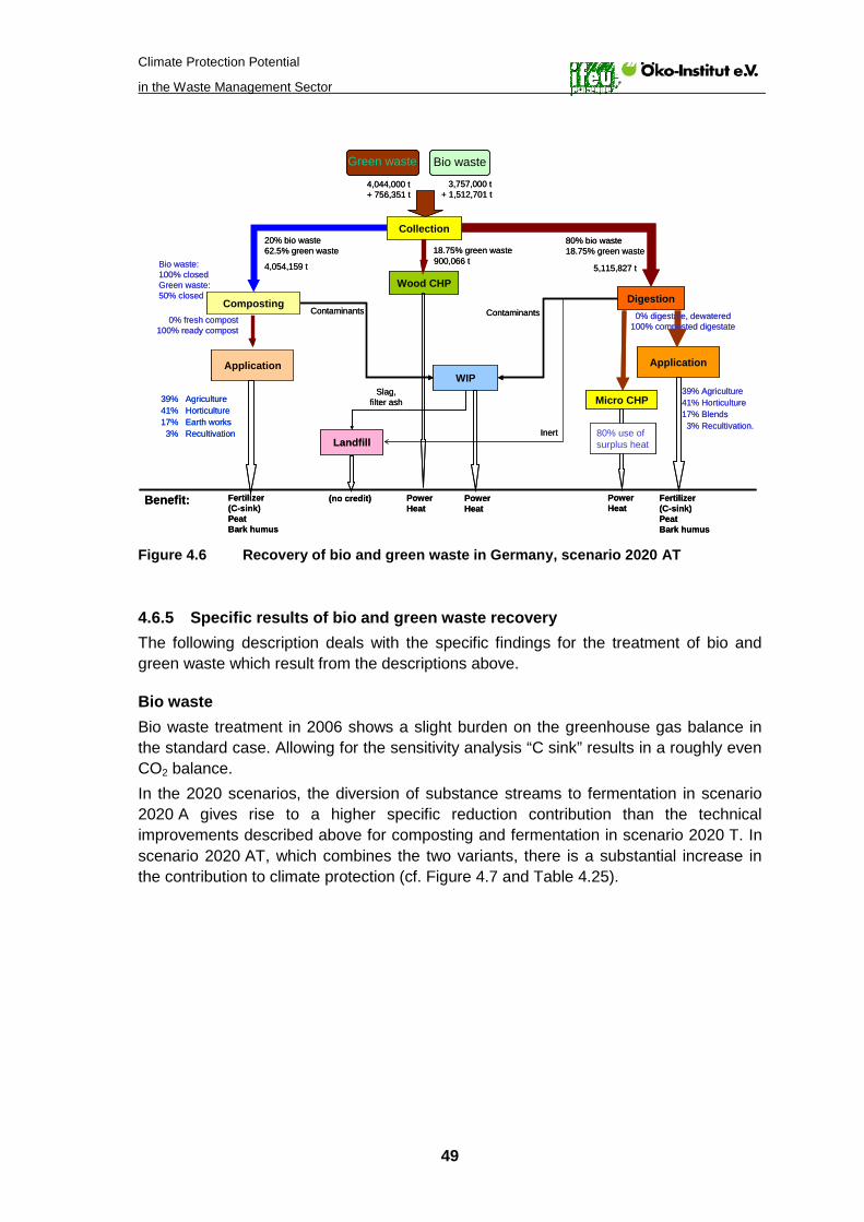
Climate Protection Potential
in the Waste Management Sector
49
Benefit:
Landfill
Slag,filter ash
WIP
Digestion
Collection
Composting
4,044,000 t+ 756,351 t
3,757,000 t+ 1,512,701 t
Contaminants Contaminants
Inert
Application Application
Wood CHP
0% fresh compost100% ready compost
0% digestate, dewatered100% composted digestate
39% Agriculture41% Horticulture17% Blends3% Recultivation.
20% bio waste62.5% green waste
5,115,827 t
80% bio waste18.75% green waste
4,054,159 t
18.75% green waste900,066 tBio waste:
100% closedGreen waste: 50% closed
80% use of surplus heat
39% Agriculture41% Horticulture17% Earth works3% Recultivation
PowerHeat
Fertilizer(C-sink)PeatBark humus
(no credit) PowerHeat
Fertilizer(C-sink)PeatBark humus
PowerHeat
Bio wasteGreen waste
Micro CHP
Figure 4.6 Recovery of bio and green waste in Germany, scenario 2020 AT
4.6.5 Specific results of bio and green waste recovery The following description deals with the specific findings for the treatment of bio and green waste which result from the descriptions above.
Bio waste Bio waste treatment in 2006 shows a slight burden on the greenhouse gas balance in the standard case. Allowing for the sensitivity analysis “C sink” results in a roughly even CO2 balance. In the 2020 scenarios, the diversion of substance streams to fermentation in scenario 2020 A gives rise to a higher specific reduction contribution than the technical improvements described above for composting and fermentation in scenario 2020 T. In scenario 2020 AT, which combines the two variants, there is a substantial increase in the contribution to climate protection (cf. Figure 4.7 and Table 4.25).

Climate Protection Potential
in the Waste Management Sector
50
Greenhouse gases, specific: Bio waste (with and without C-sink)
-300 -250 -200 -150 -100 -50 0 50 100 150
20062020 T
2020 A
2020 AT
kg CO2-eq/t input
Coll. + Trans Operation Power & Heat Compost WIP C-sink Total Plus C-sink Figure 4.7 Specific greenhouse gas emission factors for bio waste treatment, broken
down by major contributions21
Table 4.26 Specific greenhouse gas emission factors for bio waste treatment, broken down by major contributions
Greenhouse gases, specific kg CO2 eq/t
Components 2006 2020 T 2020 A 2020 AT Coll. +Trans. 10.5 10.5 10.5 10.5 Operation 79.3 85.7 76.8 47.2 Power + Heat -24.3 -29.8 -129.8 -159.0 Compost -42.7 -88.0 -0.8 -78.2 WIP -6.0 -17.0 -4.9 -15.0 EF bio waste 16.7 -38.6 -48.3 -194.5 C-sink -17.9 -14.0 -19.6 -12.2 EF bio waste with C sink -1.2 -52.7 -67.8 -206.6
There is a drop in operating emissions in scenario 2020 AT, because here the decline in composting alone (as in 2020 A) coincides with the considerable optimisation of fermentation with regard to methane emissions (as in 2020 T). The conversion from straight composting facilities in 2006 and 2020 T to combined fermentation processes with follow-up pit results in an increased credit for energy use in scenario 2020 A, and this shows a further rise in scenario 2020 AT as a result of better heat utilisation.
21Figure 4.7, Figure 4.8 and Figure 4.13 show the results of the standard balance (without hatched bar segment) and the sensitivity analysis taking account of the C sink (with the hatched bar segment) for all the scenarios.
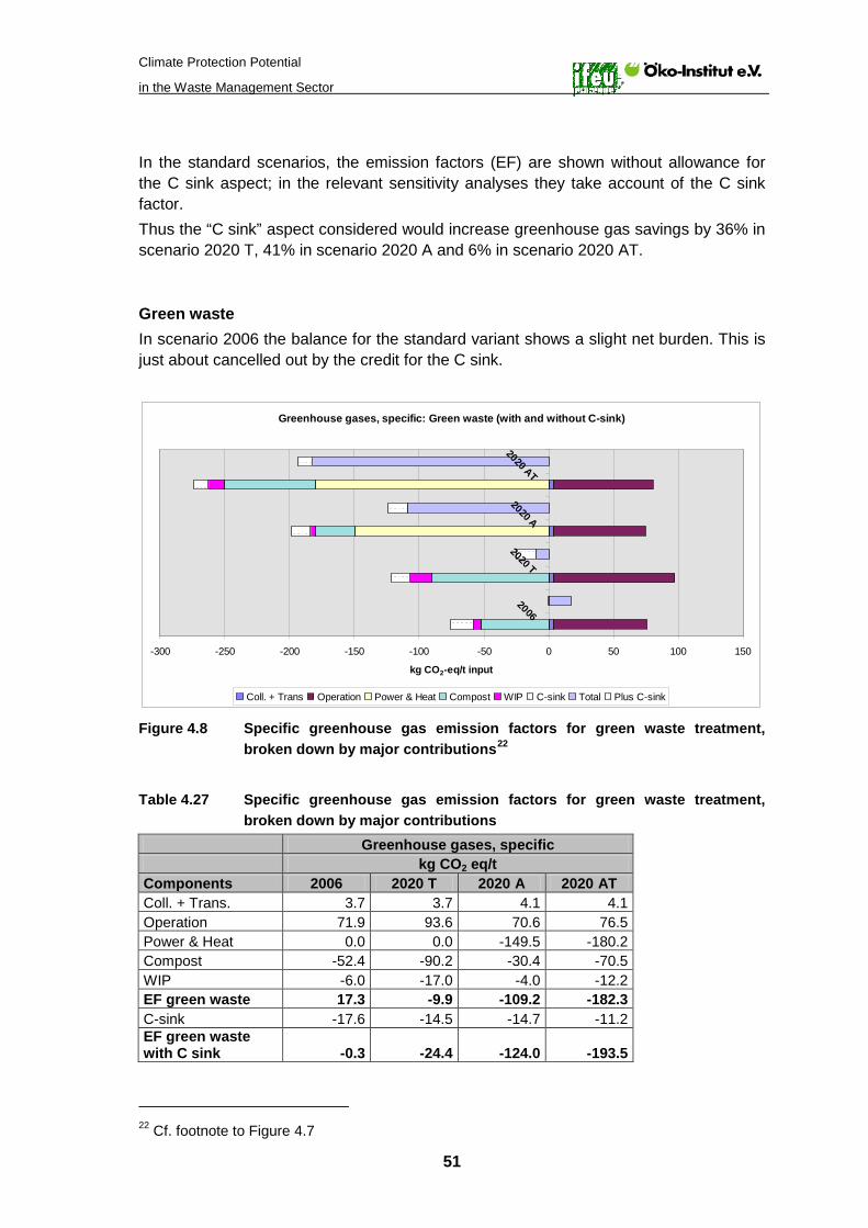
Climate Protection Potential
in the Waste Management Sector
51
In the standard scenarios, the emission factors (EF) are shown without allowance for the C sink aspect; in the relevant sensitivity analyses they take account of the C sink factor. Thus the “C sink” aspect considered would increase greenhouse gas savings by 36% in scenario 2020 T, 41% in scenario 2020 A and 6% in scenario 2020 AT.
Green waste In scenario 2006 the balance for the standard variant shows a slight net burden. This is just about cancelled out by the credit for the C sink.
Greenhouse gases, specific: Green waste (with and without C-sink)
-300 -250 -200 -150 -100 -50 0 50 100 150
2006
2020 T
2020 A
2020 AT
kg CO2-eq/t input
Coll. + Trans Operation Power & Heat Compost WIP C-sink Total Plus C-sink
Figure 4.8 Specific greenhouse gas emission factors for green waste treatment, broken down by major contributions22
Table 4.27 Specific greenhouse gas emission factors for green waste treatment, broken down by major contributions
Greenhouse gases, specific kg CO2 eq/t
Components 2006 2020 T 2020 A 2020 AT Coll. + Trans. 3.7 3.7 4.1 4.1 Operation 71.9 93.6 70.6 76.5 Power & Heat 0.0 0.0 -149.5 -180.2 Compost -52.4 -90.2 -30.4 -70.5 WIP -6.0 -17.0 -4.0 -12.2 EF green waste 17.3 -9.9 -109.2 -182.3 C-sink -17.6 -14.5 -14.7 -11.2 EF green waste with C sink -0.3 -24.4 -124.0 -193.5
22 Cf. footnote to Figure 4.7
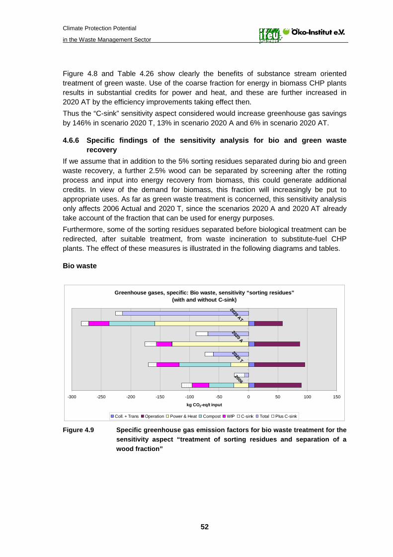
Climate Protection Potential
in the Waste Management Sector
52
Figure 4.8 and Table 4.26 show clearly the benefits of substance stream oriented treatment of green waste. Use of the coarse fraction for energy in biomass CHP plants results in substantial credits for power and heat, and these are further increased in 2020 AT by the efficiency improvements taking effect then. Thus the “C-sink” sensitivity aspect considered would increase greenhouse gas savings by 146% in scenario 2020 T, 13% in scenario 2020 A and 6% in scenario 2020 AT.
4.6.6 Specific findings of the sensitivity analysis for bio and green waste recovery
If we assume that in addition to the 5% sorting residues separated during bio and green waste recovery, a further 2.5% wood can be separated by screening after the rotting process and input into energy recovery from biomass, this could generate additional credits. In view of the demand for biomass, this fraction will increasingly be put to appropriate uses. As far as green waste treatment is concerned, this sensitivity analysis only affects 2006 Actual and 2020 T, since the scenarios 2020 A and 2020 AT already take account of the fraction that can be used for energy purposes. Furthermore, some of the sorting residues separated before biological treatment can be redirected, after suitable treatment, from waste incineration to substitute-fuel CHP plants. The effect of these measures is illustrated in the following diagrams and tables.
Bio waste
Greenhouse gases, specific: Bio waste, sensitivity “sorting residues”(with and without C-sink)
-300 -250 -200 -150 -100 -50 0 50 100 150
20062020 T
2020 A
2020 AT
kg CO2-eq/t input
Coll. + Trans Operation Power & Heat Compost WIP C-sink Total Plus C-sink Figure 4.9 Specific greenhouse gas emission factors for bio waste treatment for the
sensitivity aspect “treatment of sorting residues and separation of a wood fraction”

Climate Protection Potential
in the Waste Management Sector
53
Table 4.28 Specific greenhouse gas emission factors for bio waste treatment for the sensitivity aspect “treatment of sorting residues and separation of a wood fraction”
Greenhouse gases, specific kg CO2 eq/t
Components 2006 2020 T 2020 A 2020 AT Coll. + Trans. 10.5 10.5 10.5 10.5 Operation 79.3 85.7 76.8 47.2 Power & Heat -24.3 -29.8 -129.8 -159.0 Compost -42.7 -88.0 -0.8 -78.2 WIP -28.7 -38.1 -25.8 -34.5 EF bio waste -5.9 -59.7 -69.2 -214.0 C-sink -17.9 -14.0 -19.6 -12.2 EF bio waste with C sink -23.8 -73.8 -88.7 -226.1
Whereas bio waste treatment in the standard balance for 2006 without C sink shows a slight debit of 17 kg CO2 eq/t, after allowing for this sensitivity aspect it achieves a small credit of 6 kg CO2 eq/t as early as 2006. Bio waste treatment also displays an improvement of around 20 kg CO2 eq/t in the other scenarios as well. Thus the sensitivity analysis considered would, without taking account of the C sink aspect, increase greenhouse gas savings by 55% in scenario 2020 T, 43% in scenario 2020 A and 10% in scenario 2020 AT.
Green waste
Greenhouse gases, specific: Green waste, sensitivity “sorting residues”(with and without C-sink)
-300 -250 -200 -150 -100 -50 0 50 100 150
2006
2020 T
2020 A
2020 AT
kg CO2-eq/t input
Coll. + Trans Operation Power & Heat Compost WIP C-sink Total Plus C-sink
Figure 4.10 Specific greenhouse gas emission factors for green waste treatment for the sensitivity aspect “treatment of sorting residues and separation of a wood fraction”

Climate Protection Potential
in the Waste Management Sector
54
Table 4.29 Specific greenhouse gas emission factors for green waste treatment for the sensitivity aspect “treatment of sorting residues and separation of a wood fraction”
Greenhouse gases, specific
kg CO2 eq/t Components 2006 2020 T 2020 A 2020 AT Coll. + Trans. 3.7 3.7 4.1 4.1 Operation 71.9 93.6 70.6 76.5 Power + Heat 0.0 0.0 -149.5 -180.2 Compost -52.4 -90.2 -30.4 -70.5 WIP -28.7 -38.1 -9.3 -14.0 EF green waste -5.4 -31.0 -114.5 -184.1 C-sink -17.6 -14.5 -14.7 -11.2 EF green waste with C sink -22.9 -45.5 -129.2 -195.3
In the standard balance for 2006, composting of green waste still results in a debit of around 17 kg CO2 eq/t, which is just cancelled out by the C sink credit. For this sensitivity it shows a small credit of about 5 kg CO2 eq/t in 2006. The improvement is much the same in scenario 2020 T. Scenarios 2020 A and 2020 AT do not bring any appreciable improvement compared with the standard balance, which is already optimised for substance streams. Thus the sensitivity analysis considered would, without taking account of the C sink aspect, increase greenhouse gas savings by 146% in scenario 2020 T, 13% in scenario 2020 A and 6% in scenario 2020 AT.
4.7 Paper, board and cartons (PBC)
As far as collected quantities of paper, board and cartons are concerned, it is assumed that 50% of the paper in residual waste can be collected separately in 2020. This results in the paper, board and carton quantity increasing from 8.08 million t/a to 9.24 million t/a. In the case of waste paper there is no change in the recovery technology. After sorting, waste paper is processed and recovered in paper mills. This gives rise to reject material and paper sludge as waste. The reject material (about 0.6% of the input) is burned in waste incineration plants, and paper sludge (approx. 5.3% of the input) in coal-fired power plants. The avoidance of primary fibre production from industrial wood is applied as a credit for the waste paper fibre produced in this way. A technical substitution factor (SF) is used to take account of the fact that the secondary fibres from paper, board and cartons are of slightly lower quality than primary fibres (SF=0.95)23
Regarding the question of which primary fibres are replaced by waste paper recycling, focussing on one paper segment would not do justice to the intertwined nature of the paper market. For example, the packaging sector traditionally has a high level of waste
.
23 According to information from experimental studies by commercial recovery operations. In waste paper recycling, unlike glass, tinplate or aluminium, it is always necessary to feed a small proportion of primary fibre into the products, regardless of material losses, to ensure they perform the intended functions such as stability, tear strength etc.

Climate Protection Potential
in the Waste Management Sector
55
paper input. Reducing this would make it necessary to use new fibres in this segment24. It is more likely, however, that better quality fibres would be diverted from the graphic papers sector, where they would have to be replaced by new fibres. To determine the probable replacement of new fibres, the paper market is therefore regarded as a whole. The proportions of cellulose and/or wood material are estimated for the main segments (newsprint, magazine paper, copy paper, PBC for packaging) and weighted in accordance with the VDP25
Furthermore, the authors take the view that another aspect needs to be taken into account in the case of biogenic resources such as paper: biogenic resources are not available in unlimited quantities, and there are cases where targets for expanding renewable energy sources at German, EU and global level give rise to marked competition between uses. If waste paper is recycled, for example, it is very likely that the wood saved in this way will be used for generating energy. But even if this does not happen and the wood is left in the forest, there is a difference from fossil resources: if they remain in their reservoir, there is in fact no impact on the environment, whereas in the case of wood there is a change which influences climate protection. If forest is conserved, it changes over time and increased amounts of carbon are accumulated. In order to take account of the increasing use of biogenic resources and the climate protection contribution of wood conservation in a life cycle assessment approach, the system boundaries should be expanded to take in “raw material deposits”.
marketing figures for paper products. This results in a new fibre mix in Germany of around 57% chemical pulp and 43% mechanical pulp. There is no integrated paper production in Germany. Even if there were no waste paper, no cellulose industry would be built up, but imports would increase, so accounting for substitution at fibre level is appropriate for Germany.
In this study the standard scenario assumes that there is great pressure to use wood and that the wood saved will be used in a wood-burning CHP plant. This assumes use in Sweden as one of the main source countries for new fibre for paper manufacture. Use for energy purposes in Sweden is compared with average heat and power production there. This assumption is a deliberately conservative one, i.e. fully conscious of the fact that the resulting credits are comparatively small, since most of the electricity generated in Sweden comes from nuclear power and renewable energy sources, and even heat in household heating systems is largely due to electric heaters (approx. 80%) and oil-fired systems26
The sensitivity aspects examined below are leaving the wood in the forests (“conservation”), and the assumption that the wood is imported into Germany and used there in wood-burning CHP plants (“energy D”). As a credit for the latter, the marginal
.
24 When produced from primary material, paper, board and carton for packaging consist of roughly 70% chemical pulp and 30% mechanical pulp. 25 Verband Deutscher Papierfabriken e.V. (Association of German Paper Mills): Leistungsbericht Papier (Paper Performance Report), published annually 26 Here we are concerned with the energy mixes in Sweden with large proportions of electricity and heat from renewable and nuclear sources, and not – as with the other credits in this balance – the replacement of entirely fossil energy sources. If one attempted to generate fossil mixes for Sweden, which would hardly be in line with the real situation in Sweden, the result would correspond roughly to the sensitivity aspect of transporting the wood to Germany.

Climate Protection Potential
in the Waste Management Sector
56
power and marginal heat is allocated according to the BMU method as in the standard scenario. Where the wood remains in the forest, a conservative estimate of 0.8 t C/t industrial wood is made on the basis of IFC Consulting (2006) and depreciated over the usual period of 20 years.
4.7.1 Specific findings for recovery of paper, board and cartons The following description deals with the specific findings for the recovery of paper, board and cartons which result from the descriptions above. In addition to the contribution for the provision of waste paper and the replacement of production from primary raw materials (coll. + trans, paper recycling, waste incineration), the credit for the wood saved accounts for a relevant proportion of this result (transport of wood, input for wood, power from wood, heat from wood), especially in the technically optimised scenarios with increased heat offtake from wood-burning CHP plants.
Greenhouse gases, specific: PBC (use of wood for energy in Sweden)
-1200 -1000 -800 -600 -400 -200 0 200 400
2006
2020 T
2020 A
2020 AT
kg CO2-eq/t input
Coll. + Trans. Paper Recycling WIP Trans: wood Input wood Power wood Heat wood Total
Figure 4.11 Specific greenhouse gas emission factors for paper, board and cartons, broken down by major contributions

Climate Protection Potential
in the Waste Management Sector
57
Table 4.30 Specific greenhouse gas emission factors for paper, board and cartons, broken down by major contributions
Greenhouse gases, specific kg CO2 eq/t
Components 2006 2020 T 2020 A 2020 AT Coll. + Trans. 33.8 33.8 33.8 33.8 Paper recycling* -706.6 -706.6 -706.6 -706.6 WIP -1.2 -3.4 -1.0 -3.0 Transport of wood 41.9 41.9 41.9 41.9 Input for wood** 107.4 107.4 107.4 107.4 Power from wood -50.6 -45.5 -50.6 -45.5 Heat from wood -156.2 -312.4 -156.2 -312.4 EF PBC -731.5 -884.8 -731.3 -884.4
* Net credit (input minus credit) for paper recycling ** Effort involved in supplying and transporting wood
4.7.2 Specific findings of sensitivity analysis for recovery of paper, board and cartons
The credit for the wood savings depends heavily on whether the wood remains in the forest or whether it is assumed to be used for energy purposes. The effect is even greater if one compares different use scenarios. The credits generated are smallest if the wood is used in Sweden and if, contrary to the assumptions for other energy supplied, only the normal power mix is balanced there (standard balance, “energy S”). In Sweden, electricity and heat are to a large extent generated from non-fossil energy sources.
Greenhouse gases, specific: PBC 202 AT – sensitivity “variation wood credits”
-3000 -2500 -2000 -1500 -1000 -500 0 500
Energy S
Energy D
Conservation
No wood CR
kg CO2-eq/t input
Coll. + Trans. Paper Recycling WIP Trans: wood Input wood Power wood Heat wood Total
Figure 4.12 Various sensitivities in relation to use of wood saved by paper recycling in the scenario 2020 AT
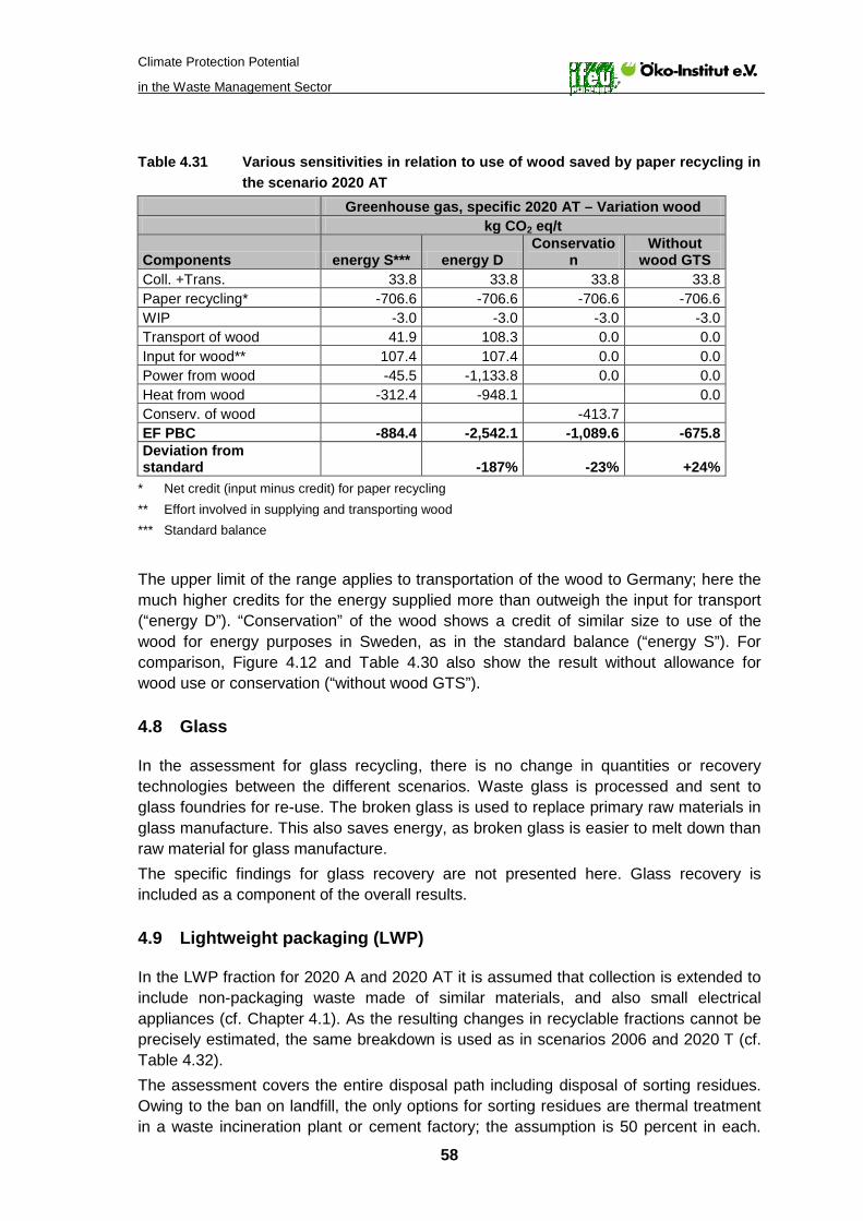
Climate Protection Potential
in the Waste Management Sector
58
Table 4.31 Various sensitivities in relation to use of wood saved by paper recycling in the scenario 2020 AT
Greenhouse gas, specific 2020 AT – Variation wood kg CO2 eq/t
Components energy S*** energy D Conservatio
n Without
wood GTS Coll. +Trans. 33.8 33.8 33.8 33.8 Paper recycling* -706.6 -706.6 -706.6 -706.6 WIP -3.0 -3.0 -3.0 -3.0 Transport of wood 41.9 108.3 0.0 0.0 Input for wood** 107.4 107.4 0.0 0.0 Power from wood -45.5 -1,133.8 0.0 0.0 Heat from wood -312.4 -948.1 0.0 Conserv. of wood -413.7 EF PBC -884.4 -2,542.1 -1,089.6 -675.8 Deviation from standard -187% -23% +24%
* Net credit (input minus credit) for paper recycling ** Effort involved in supplying and transporting wood *** Standard balance
The upper limit of the range applies to transportation of the wood to Germany; here the much higher credits for the energy supplied more than outweigh the input for transport (“energy D”). “Conservation” of the wood shows a credit of similar size to use of the wood for energy purposes in Sweden, as in the standard balance (“energy S”). For comparison, Figure 4.12 and Table 4.30 also show the result without allowance for wood use or conservation (“without wood GTS”).
4.8 Glass
In the assessment for glass recycling, there is no change in quantities or recovery technologies between the different scenarios. Waste glass is processed and sent to glass foundries for re-use. The broken glass is used to replace primary raw materials in glass manufacture. This also saves energy, as broken glass is easier to melt down than raw material for glass manufacture. The specific findings for glass recovery are not presented here. Glass recovery is included as a component of the overall results.
4.9 Lightweight packaging (LWP)
In the LWP fraction for 2020 A and 2020 AT it is assumed that collection is extended to include non-packaging waste made of similar materials, and also small electrical appliances (cf. Chapter 4.1). As the resulting changes in recyclable fractions cannot be precisely estimated, the same breakdown is used as in scenarios 2006 and 2020 T (cf. Table 4.32). The assessment covers the entire disposal path including disposal of sorting residues. Owing to the ban on landfill, the only options for sorting residues are thermal treatment in a waste incineration plant or cement factory; the assumption is 50 percent in each.

Climate Protection Potential
in the Waste Management Sector
59
The composition of the waste is simplified in line with the average composition of substitute fuels shown in Table 4.10. The breakdown of constituents in the LWP fraction is adopted from IFEU (2006) (cf. Table 4.31). Liquid cartons and other composites are essentially made of paper and are recovered like paper in paper factories. This too conserves wood. For waste paper in the standard scenario it is assumed, in view of the pressure on uses in Sweden, that the quantity of industrial wood saved is used in a wood-burning CHP plant. Table 4.32 Breakdown of LWP into recyclable fractions and sorting residues* (IFEU 2006)
Shares in % Plastics 36.0 Tinplate 11.7 Aluminium 1.7 LC 5.0 Other composites 5.3 Residues 40.3 Total 100.0
* Used for all scenarios even after extension to include non-packaging waste and small electrical appliances
The further breakdown of plastics (Table 4.32) uses the distribution of recyclable fractions according to IFEU/HTP (2001). Table 4.33 Breakdown of plastics into recyclable fractions (IFEU/HTP 2001)
Shares in % Film 18.3 Mixed plastics 65.0 Bottles 14.7 Tubs 2.0 Miscellaneous 0 100.0 The further recycling of plastic fractions is modelled on IFEU/HTP (2001). The relevant figures for yields and substitution potentials of recovery as materials are listed in Table 4.33. For the bottle fraction it is assumed that 10% are PET bottles (shown separately in Table 4.33) and the rest consists of equal amounts of PE and PP bottles. It is assumed that the treatment residues resulting from recovery of plastic as materials are sent for co-incineration in cement factories. The combustion parameters used are the data shown in Table 4.10 as a weighted mean for substitute fuels.

Climate Protection Potential
in the Waste Management Sector
60
Table 4.34 Yields and substitution potentials used for recovery as material in scenarios 2006 and 2020 A
(after IFEU/HTP 2001)
Film Bottles Tubs PET MP SF % % % % % Treatment residue 21 17 23 25 10 Water 15 1 6 PET 1.0 75 Plastic substitute PO 0.9 5 1 Regrind PO 0.7 60 67 30 Regrind PP 0.9 14 Regrind PS 0.9 56 Palisades wood 7 3 27 Palisades concrete 7 3 27
SF = substitution factor
A proportion of mixed plastics is also recovered as energy. At the time of the IFEU/HTP (2001) study the proportion of recovery as energy was very high, at 95%. According to recyclers, however, the thermal recovery figure for 2006 can be expected to be very much lower, at 50%. This is the figure used in this study. Use in blast furnaces or cement factories is a possibility for recovery of mixed plastics as energy. A 50:50 split is assumed (cf. also Öko-Institut 1999 and Jenseit 1995). In scenarios 2020 T and 2020 AT it is assumed that there are possibilities for higher-grade use of the secondary plastics produced through recovery as material. For these it is assumed that only primary plastics are replaced – in other words as a general rule no longer the primary products wood and concrete palisades, which are made of different materials. Furthermore, a substitution factor of 0.9 is generally used for secondary products from films, bottles and tubs (substitute plastic or regrind), and a substitution factor of 0.7 for secondary products from mixed plastics (regrind PO). In view of the fact that treatment technologies and the recycling market have undergone further development since the collection of the IFEU/HTP (2001) project data, this assumption would seem appropriate (cf. also Öko-Institut 2001 and 2002a). The uses of the 50% mixed plastics recovered as energy are the same as in 2006.
4.9.1 Specific findings for recovery of lightweight packaging (LWP) The following description deals with the specific findings for lightweight packaging recovery which result from the descriptions above. The balance for LWP shows separately the credit for the wood used in Sweden which is saved by recycling liquid cartons and other composites containing paper, board and cartons (“Wood GTS”).
Climate Protection Potential
in the Waste Management Sector
61
Greenhouse gases, specific: LWP(with and without wood credit for liquid cartons and other composites)
-900 -750 -600 -450 -300 -150 0 150
20062020 T
2020 A
2020 AT
kg CO2-eq/t input
Coll.+ Trans. Operation Material Energy WIP Wood CR Total Plus wood CR
Figure 4.13 Specific greenhouse gas emission factors for lightweight packaging, broken down by major contributions27
Table 4.35 Specific greenhouse gas emission factors for lightweight packaging, broken down by major contributions
Greenhouse gases, specific kg CO2 eq/t
Components 2006 2020 T 2020 A 2020 AT Coll. +Trans. 47.8 47.8 47.8 47.8 Operation 56.1 56.1 56.1 56.1 as Material -345.5 -470.1 -345.5 -470.1 as Energy -207.7 -210.6 -207.7 -210.6 WIP 6.0 -57.7 6.0 -57.7 EF LWP without wood GTS -443.3 -634.4 -443.3 -634.4 Plus wood GTS -53.6 -106.6 -55.9 -106.6 EF LWP -496.9 -734.1 -499.2 -734.1
The substitution effects resulting from the recovery of separately collected substances as materials and energy – such as substitution of primary plastics and primary energy sources – far outweigh the input for collection and transport and the operation of the treatment plants. On present standards the sorting residues, half of which are burned in waste incineration plants and half in cement factories, can only yield net relief if used for co-incineration in cement factories (included in total for “as energy”). Combustion in waste incineration plants does not result in a net credit in 2006 Actual and 2020 A, as the fossil
27 Cf. footnote to Figure 4.7. Here the hatched parts of the bars represent the wood credit resulting from use of the wood quantities conserved by recycling liquid cartons and paper composites (as part of the standard balance, as in the case of paper, board and cartons). The balance is based on the same procedure as for paper, board and cartons.
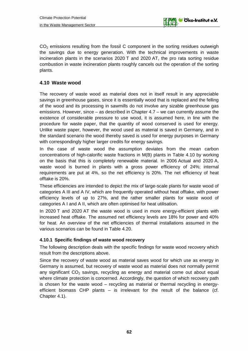
Climate Protection Potential
in the Waste Management Sector
62
CO2 emissions resulting from the fossil C component in the sorting residues outweigh the savings due to energy generation. With the technical improvements in waste incineration plants in the scenarios 2020 T and 2020 AT, the pro rata sorting residue combustion in waste incineration plants roughly cancels out the operation of the sorting plants.
4.10 Waste wood
The recovery of waste wood as material does not in itself result in any appreciable savings in greenhouse gases, since it is essentially wood that is replaced and the felling of the wood and its processing in sawmills do not involve any sizable greenhouse gas emissions. However, since – as described in Chapter 4.7 – we can currently assume the existence of considerable pressure to use wood, it is assumed here, in line with the procedure for waste paper, that the quantity of wood conserved is used for energy. Unlike waste paper, however, the wood used as material is saved in Germany, and in the standard scenario the wood thereby saved is used for energy purposes in Germany with correspondingly higher larger credits for energy savings. In the case of waste wood the assumption deviates from the mean carbon concentrations of high-calorific waste fractions in M(B) plants in Table 4.10 by working on the basis that this is completely renewable material. In 2006 Actual and 2020 A, waste wood is burned in plants with a gross power efficiency of 24%; internal requirements are put at 4%, so the net efficiency is 20%. The net efficiency of heat offtake is 20%. These efficiencies are intended to depict the mix of large-scale plants for waste wood of categories A III and A IV, which are frequently operated without heat offtake, with power efficiency levels of up to 27%, and the rather smaller plants for waste wood of categories A I and A II, which are often optimised for heat utilisation. In 2020 T and 2020 AT the waste wood is used in more energy-efficient plants with increased heat offtake. The assumed net efficiency levels are 18% for power and 40% for heat. An overview of the net efficiencies of thermal installations assumed in the various scenarios can be found in Table 4.20.
4.10.1 Specific findings of waste wood recovery The following description deals with the specific findings for waste wood recovery which result from the descriptions above. Since the recovery of waste wood as material saves wood for which use as energy in Germany is assumed, but recovery of waste wood as material does not normally permit any significant CO2 savings, recycling as energy and material come out about equal where climate protection is concerned. Accordingly, the question of which recovery path is chosen for the waste wood – recycling as material or thermal recycling in energy-efficient biomass CHP plants – is irrelevant for the result of the balance (cf. Chapter 4.1).

Climate Protection Potential
in the Waste Management Sector
63
Greenhouse gases, specific: Waste wood
-1400 -1200 -1000 -800 -600 -400 -200 0 200
2006
2020 T
2020 A
2020 AT
kg CO2-eq/t input
Coll.+ Trans. Material Operation incin. Power Heat Wood CR Total
Figure 4.14 Specific greenhouse gas emission factors for waste wood, broken down by major contributions
Table 4.36 Specific greenhouse gas emission factors for waste wood, broken down by major contributions
Greenhouse gases, specific kg CO2 eq/t
Components 2006 2020 T 2020 A 2020 AT Coll. +Trans. 6.9 6.9 6.7 6.7 as Material -3.7 -3.7 -3.5 -3.5 WIP operation 41.6 41.6 42.5 42.5 Electricity -504.9 -454.4 -516.1 -464.5 Heat -190.0 -380.0 -194.2 -388.5 Wood GTS -292.3 -354.9 -278.3 -337.9 EF waste wood -942.4 -1,144.5 -943.0 -1,145.2
The technical improvements are due to the better heat production from the combustion of wood. Since the absolute quantity of wood recycling as material is not increasing, despite the additional quantities in the scenarios 2020 A and 2020 AT, its share of the total is declining. As a result, the specific findings also show a reduction in the greenhouse gas emissions for collection and transport and the credits for “as energy” and wood-GTS, while there is a corresponding increase in the share of EF waste wood accounted for by energy modules.

Climate Protection Potential
in the Waste Management Sector
64
5 Overall results of the standard balance
This chapter describes the overall results of the standard balance for greenhouse gases (GG) and energy resources (CED fossil) in accordance with the framework conditions described. The overall results for greenhouse gases are the product of the specific results already explained in Chapters 4.3 to 4.10 and the relevant absolute waste quantities. The same applies to the conservation of fossil resources, expressed as the cumulative energy demand (CED fossil), for which no specific individual results are presented (cf. also Chapter 3.2). The standard balance results are followed by a summary description of the overall contribution of waste incineration plants (cf. Chapter 5.3), since the accounting method means that the overall results only show the contribution of waste incineration in respect of the residual waste delivered directly to waste incineration plants. The sensitivity analyses follow in Chapter 6. The overall results are shown for the scenarios described in Chapter 4 and the waste streams set out in Table 4.2 and Figure 5.1.
Destination
0
5,000
10,000
15,000
20,000
25,000
30,000
35,000
40,000
45,000
50,000
2006 Actual 2020 T 2020 A 2020 AT
1,00
0 t/a
Waste WoodLWPGlassPBCGreen wasteBio wasteMBT/MBS/MTWIPLandfill
Figure 5.1 Waste streams (destination) of the scenarios examined
5.1 Greenhouse gases (GG)
Figure 5.2 and Table 5.1 show the overall balance results for greenhouse gases. It will be seen that the effects of the technical improvements applied result in a greater increase in greenhouse gas emission savings than the change in waste streams alone. The biggest savings are achieved through recycling of paper, board and cartons (PBC) and waste wood, followed by LWP recycling and waste incineration. The savings due to PBC, LWP (liquid cartons and other composites) and waste wood in each case include the savings arising from wood saved (cf. Chapters 4.7, 4.9 and 4.10). In the standard case this is the credit for use of the wood for energy purposes in Sweden. This involves

Climate Protection Potential
in the Waste Management Sector
65
relatively small credits, since the average energy generation in Sweden which is credited here is largely the result of renewable or nuclear energy (cf. Figure 4.12).
Greenhouse gases, total
-30,000
-25,000
-20,000
-15,000
-10,000
-5,000
0
5,000
1,00
0 t C
O2/a
Waste WoodLWPGlassPBCGreen wasteBio wasteMBT/MBS/MTWIPLandfill
2006 Actual 2020 T 2020 A 2020 AT
Figure 5.2 Overall results of standard balance for greenhouse gases28
Table 5.1 Overall results of standard balance for greenhouse gases
2006
Actual 2020 T 2020 A 2020 AT
1,000 t
CO2 eq/a 1,000 t
CO2 eq/a 1,000 t
CO2 eq/a 1,000 t
CO2 eq/a Landfill 62 0 0 0 WIP -1,407 -4,038 -799 -2,497 M(B) plants -1,000 -1,971 -637 -1,364 Bio waste 62,9 -145 -254 -1,025 Green waste 70 -40 -524 -875 PBC -5,911 -7,149 -6,758 -8,173 Glass -897 -897 -897 -897 LWP -2,252 -3,358 -2,923 -4,339 Waste wood -6,503 -7,897 -6,834 -8,299 Total -17,773 -25,496 -19,625 -27,468
For the municipal waste sector in Germany the scenario 2006 Actual already shows a reduction in greenhouse gas emissions by around 18 million t CO2 eq/a for 2006. To put this in perspective: a comparison of this quantity with car traffic in Germany shows that on the basis of current average emission levels per car of around 180 g CO2/km and an average mileage of around 13,000 km/a, the reductions achieved by the German
28 This and the following figures summarise the contributions of the waste sector as a whole and its individual sectors. Figures with a minus sign indicate a contribution to relieving the climate situation. Positive figures, where present, indicate additional burdens on the climate situation.
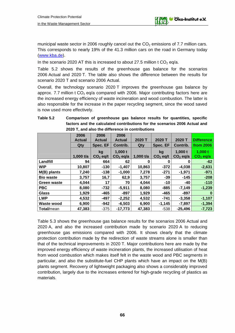
Climate Protection Potential
in the Waste Management Sector
66
municipal waste sector in 2006 roughly cancel out the CO2 emissions of 7.7 million cars. This corresponds to nearly 19% of the 41.3 million cars on the road in Germany today (www.kba.de). In the scenario 2020 AT this is increased to about 27.5 million t CO2 eq/a. Table 5.2 shows the results of the greenhouse gas balance for the scenarios 2006 Actual and 2020 T. The table also shows the difference between the results for scenario 2020 T and scenario 2006 Actual. Overall, the technology scenario 2020 T improves the greenhouse gas balance by approx. 7.7 million t CO2 eq/a compared with 2006. Major contributing factors here are the increased energy efficiency of waste incineration and wood combustion. The latter is also responsible for the increase in the paper recycling segment, since the wood saved is now used more effectively.
Table 5.2 Comparison of greenhouse gas balance results for quantities, specific factors and the calculated contributions for the scenarios 2006 Actual and 2020 T, and also the difference in contributions
2006 Actual
2006 Actual
2006 Actual 2020 T 2020 T 2020 T Difference
Qty Spec. EF Contrib. Qty Spec. EF Contrib. from 2006
1,000 t/a kg
CO2 eq/t 1,000 t
CO2 eq/a 1,000 t/a kg
CO2 eq/t 1,000 t
CO2 eq/a 1,000 t
CO2 eq/a Landfill 94 664 62 0 0 0 -62 WIP 10,807 -130 -1,407 10,863 -372 -4,038 -2,631 M(B) plants 7,240 -138 -1,000 7,278 -271 -1,971 -971 Bio waste 3,757 16,7 62,9 3,757 -39 -145 -208 Green waste 4,044 17 70 4,044 -10 -40 -110 PBC 8,080 -732 -5,911 8,080 -885 -7,149 -1,239 Glass 1,929 -465 -897 1,929 -465 -897 0 LWP 4,532 -497 -2,252 4,532 -741 -3,358 -1,107 Waste wood 6,900 -942 -6,503 6,900 -1,145 -7,897 -1,394 Total/mean 47,383 -375 -17,773 47,383 -538 -25,496 -7,723
Table 5.3 shows the greenhouse gas balance results for the scenarios 2006 Actual and 2020 A, and also the increased contribution made by scenario 2020 A to reducing greenhouse gas emissions compared with 2006. It shows clearly that the climate protection contribution made by the redirection of waste streams alone is smaller than that of the technical improvements in 2020 T. Major contributions here are made by the improved energy efficiency of waste incineration plants, the increased utilisation of heat from wood combustion which makes itself felt in the waste wood and PBC segments in particular, and also the substitute-fuel CHP plants which have an impact on the M(B) plants segment. Recovery of lightweight packaging also shows a considerably improved contribution, largely due to the increases entered for high-grade recycling of plastics as materials.

Climate Protection Potential
in the Waste Management Sector
67
Table 5.3 Comparison of greenhouse gas balance results for quantities, specific factors and the calculated contributions for the scenarios 2006 Actual and 2020 A, and also the difference in contributions
2006 Actual
2006 Actual
2006 Actual 2020 A 2020 A 2020 A Difference
Qty Spec. EF Contrib. Qty Spec. EF Contrib. from 2006
1,000 t/a kg
CO2 eq/t 1,000 t
CO2 eq/a 1,000 t/a kg
CO2 eq/t 1,000 t
CO2 eq/a 1,000 t
CO2 eq/a Landfill 94 664 62 0 0 0 -62 WIP 10,807 -130 -1,407 7,809 -102 -799 608 M(B) plants 7,240 -138 -1,000 5,229 -122 -637 363 Bio waste 3,757 16,7 62,9 5,270 -48 -254 -317 Green waste 4,044 17 70 4,800 -109 -524 -594 PBC 8,080 -732 -5,911 9,241 -731 -6,758 -847 Glass 1,929 -465 -897 1,929 -465 -897 0 LWP 4,532 -497 -2,252 5,855 -499 -2,923 -671 Waste wood 6,900 -942 -6,503 7,247 -943 -6,834 -331 Total/mean 47,383 -375 -17,773 47,381 -414 -19,625 -1,852
The comparison between the scenarios 2006 Actual and 2020 AT can be seen in Table 5.4. As expected, the increase in the contribution to greenhouse gas emission reductions corresponds approximately to the sum of the individual contributions in the scenarios 2020 T and 2020 A. In line with the changes in waste streams, the share of improvements accounted for by waste incineration is down, and there is a corresponding increase in the shares due to combustion of waste wood and recycling as material. Table 5.4 Comparison of greenhouse gas balance results for quantities, specific
factors and the calculated contributions for the scenarios 2006 Actual and 2020 AT, and also the difference in contributions
2006 Actual
2006 Actual
2006 Actual 2020 AT 2020 AT 2020 AT Difference
Qty Spec. EF Contrib. Qty Spec. EF Contrib. from 2006
1,000 t/a kg
CO2 eq/t 1,000 t
CO2 eq/a 1,000 t/a kg
CO2 eq/t 1,000 t
CO2 eq/a 1,000 t
CO2 eq/a Landfill 94 664 62 0 0 0 -62 WIP 10,807 -130 -1,407 7,809 -320 -2,497 -1,090 M(B) plants 7,240 -138 -1,000 5,229 -261 -1,364 -364 Bio waste 3,757 16,7 62,9 5,270 -194 -1,025 -1,088 Green waste 4,044 17 70 4,800 -182 -875 -945 PBC 8,080 -732 -5,911 9,241 -884 -8,173 -2,262 Glass 1,929 -465 -897 1,929 -465 -897 0 LWP 4,532 -497 -2,252 5,855 -741 -4,339 -2,087 Waste wood 6,900 -942 -6,503 7,247 -1,145 -8,299 -1,796 Total/mean 47,383 -375 -17,773 47,381 -580 -27,468 -9,695

Climate Protection Potential
in the Waste Management Sector
68
Figure 5.3 provides a comparative view of the differences between the overall climate protection contributions (totals) of the scenarios 2020 T, 2020 A and 2020 AT in relation to 2006 Actual.
-10,000
-8,000
-6,000
-4,000
-2,000
0
2020 T 2020 A 2020 AT
1.00
0 t C
O2-
eq/a
Contributions to greenhouse gas reductionDifferences from 2006
Figure 5.3 Contributions of the municipal waste sector in Germany to reducing
greenhouse gas emissions, shown as differences between the 2020 scenarios examined and 2006
Table 5.5 summarises the specific greenhouse gas emission factors (EF) of the individual waste treatment modules for the scenarios investigated. A comparison of the scenarios 2006 Actual with 2020 A and 2020 T with 2020 AT reveals that the changes in waste streams also have an influence on the specific emission factors of certain modules. For example, the removal of various recyclable materials (especially bio and green waste, paper and waste wood) results in a slight drop in the calorific value and the proportion of renewable carbon in the residual waste, leading to a corresponding reduction in the specific emission factor of waste incineration. This effect is reinforced by the reduction in the proportion of metals in residual waste due to the separate collection of metals (cf. Chapter 4.4.1). The same effects lead to a reduction in specific emission factors in the case of M(B) plants as well. This is slightly smaller than for waste incineration plants, since the changes in the breakdown of input in favour of MBS lead in turn to a pro rata increase in the specific emission factors. In the absolute results (cf. Table 5.1), this effect is even more marked because of the simultaneous decrease in the quantities for waste incineration and M(B) plants.
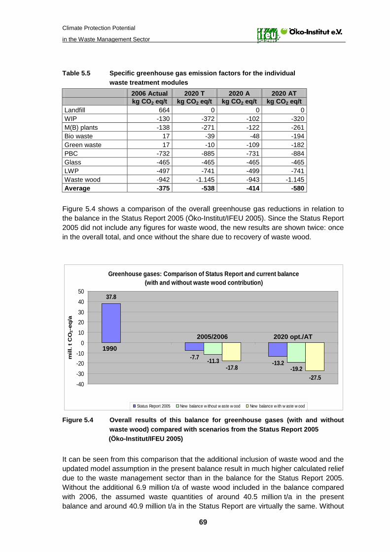
Climate Protection Potential
in the Waste Management Sector
69
Table 5.5 Specific greenhouse gas emission factors for the individual waste treatment modules
2006 Actual 2020 T 2020 A 2020 AT kg CO2 eq/t kg CO2 eq/t kg CO2 eq/t kg CO2 eq/t Landfill 664 0 0 0 WIP -130 -372 -102 -320 M(B) plants -138 -271 -122 -261 Bio waste 17 -39 -48 -194 Green waste 17 -10 -109 -182 PBC -732 -885 -731 -884 Glass -465 -465 -465 -465 LWP -497 -741 -499 -741 Waste wood -942 -1.145 -943 -1.145 Average -375 -538 -414 -580
Figure 5.4 shows a comparison of the overall greenhouse gas reductions in relation to the balance in the Status Report 2005 (Öko-Institut/IFEU 2005). Since the Status Report 2005 did not include any figures for waste wood, the new results are shown twice: once in the overall total, and once without the share due to recovery of waste wood.
Greenhouse gases: Comparison of Status Report and current balance(with and without waste wood contribution)
-13.2
37.8
-7.7
-19.2-11.3
-27.5-17.8
-40
-30
-20-10
0
10
2030
40
50
mill
. t C
O2-
eq/a
Status Report 2005 New balance w ithout w aste w ood New balance w ith w aste w ood
Figure 5.4 Overall results of this balance for greenhouse gases (with and without waste wood) compared with scenarios from the Status Report 2005 (Öko-Institut/IFEU 2005)
It can be seen from this comparison that the additional inclusion of waste wood and the updated model assumption in the present balance result in much higher calculated relief due to the waste management sector than in the balance for the Status Report 2005. Without the additional 6.9 million t/a of waste wood included in the balance compared with 2006, the assumed waste quantities of around 40.5 million t/a in the present balance and around 40.9 million t/a in the Status Report are virtually the same. Without
1990
2005/2006 2020 opt./AT

Climate Protection Potential
in the Waste Management Sector
70
the waste wood contribution, the overall contributions to reduction of greenhouse gas emissions are already very similar. The remaining differences in the form of an increase of approx. 3.6 million t CO2 eq/a for 2006 and approx. 6 million t CO2 eq/a for 2020 are due in particular to the inclusion of the wood saved by waste paper recycling (cf. Chapters 4.7, 4.9 and 4.10) and several adjustments to the framework conditions for recycling as material which were not included in the balance in the Status Report 2005 (cf. Chapter 4). Compared with the burden of 37.8 million t CO2 eq/a determined for 1990 in the Status Report 2005, the relief of 11.3 million t CO2 eq/a calculated for 2006 (disregarding the waste wood component) results in a reduction contribution of 49.1 million t CO2 eq/a (difference between the two years compared). In the scenario 2020 AT the reduction in greenhouse gas emissions is even higher, with a further 7.9 million t CO2 eq/a. Compared with 1990, the difference in the reduction contribution in 2020 thus works out at 57 million t CO2 eq/a.
5.2 Fossil energy resources
As might be expected, fossil energy resources show a similar picture to greenhouse gases where absolute totals are concerned (cf. Figure 5.5 and Table 5.6). The results for individual waste treatment modules show slight increases in the shares due to M(B) plants and waste incineration. In particular, the recycling of lightweight packaging accounts for a large proportion of the total relief, despite the small quantities. In the scenario 2020 AT, thanks to the combination of increased quantities (2020 A) with greater substitution of primary plastics (2020 T), it makes the largest contribution to saving fossil energy resources, followed by waste wood and paper, board and cartons. Overall, the municipal waste sector in Germany, including waste wood recovery, already contributes approx. 325 PJ/a to saving fossil energy resources. In the scenario 2020 AT this contribution increases to 455 PJ/a. In 2006 the total consumption of fossil primary energy in Germany came to about 12,000 PJ (DIW 2007). Given 82.4 million people in Germany, this represents an average consumption of 146 GJ per person per year. On this basis, the contribution of the municipal waste sector and waste wood recovery in 2006 corresponds to the average consumption of about 2 million persons. If one translates the savings from the scenario 2020 AT into present-day average consumption per head of the population, they make it possible to meet the requirements of 3 million people.

Climate Protection Potential
in the Waste Management Sector
71
CEDfossil, total
-500,000
-450,000
-400,000
-350,000
-300,000
-250,000
-200,000
-150,000
-100,000
-50,000
0
50,000
TJ/a
Waste WoodLWPGlassPBCGreen wasteBio wasteMBT/MBS/MTWIPLandfill
2006 Actual 2020 T 2020 A 2020 AT
Figure 5.5 Overall results of standard balance for fossil energy resources Table 5.6 Overall results of standard balance for fossil energy resources
2006
Actual 2020 T 2020 A 2020 AT TJ/a TJ/a TJ/a TJ/a Landfill 26 0 0 0 WIP -64,766 -95,826 -43,080 -63,443 M(B) plants -31,436 -43,250 -20,802 -29,667 Bio waste -591 -1,444 -7,533 -10,642 Green waste -572 -825 -8,546 -11,251 PBC -69,266 -85,550 -79,175 -97,778 Glass -7,037 -7,037 -7,037 -7,037 LWP -71,927 -98,785 -93,101 -127,625 Waste wood -79,140 -102,433 -83,164 -107,641 Total -324,708 -435,148 -342,436 -455,083
The specific emission factors for CEDfossil can be seen in Table 5.7.

Climate Protection Potential
in the Waste Management Sector
72
Table 5.7 Specific emission factors of the individual waste treatment modules for fossil energy resources (CEDfossil)
2006
Actual 2020 T 2020 A 2020 AT MJ/t MJ/t MJ/t MJ/t Landfill 276 0 0 0 WIP -5,993 -8,821 -5,517 -8,124 M(B) plants -4,342 -5,943 -3,978 -5,673 Bio waste -157 -384 -1,429 -2,019 Green waste -141 -204 -1,780 -2,344 PBC -8,573 -10,588 -8,568 -10,581 Glass -3,648 -3,648 -3,648 -3,648 LWP -15,871 -21,797 -15,901 -21,797 Waste wood -11,470 -14,845 -11,475 -14,853 Average -6,853 -9,184 -7,227 -9,605
A comparison with the results of the Status Report 2005 shows similar differences to the greenhouse gases balance. Here too the recovery of waste wood and the wood saved as a result of paper recycling account for a significant share.
CEDfossil: Comparison of Status Report and current balance(with and without waste wood contribution)
-46
-189
-260-246
-347-325
-455-500
-450
-400
-350
-300
-250
-200
-150
-100
-50
01990 2005/2006 2020 opt./AT
PJ/a
Status Report 2005 New balance without waste wood New balance with waste wood
Figure 5.6 Overall results of this balance for fossil energy resources (with and without waste wood) compared with the corresponding scenarios from the Status Report 2005 (Öko-Institut/IFEU 2005)
5.3 Overall greenhouse gas contribution of waste incineration plants
Since the balance for waste incineration plants shows only the direct inputs of residual waste, it has to be pointed out that such plants handle not only this waste stream, but also other waste quantities. A large proportion of this is commercial waste, which is not the subject of this study.
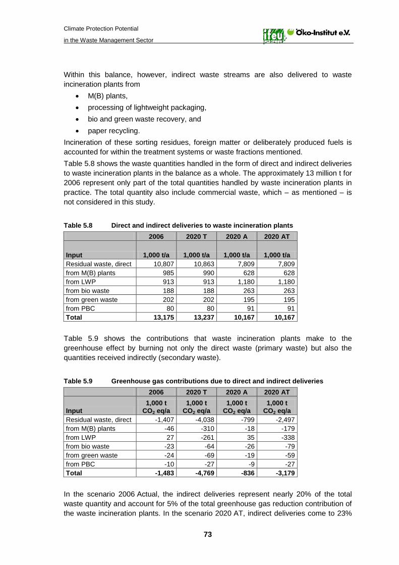
Climate Protection Potential
in the Waste Management Sector
73
Within this balance, however, indirect waste streams are also delivered to waste incineration plants from
• M(B) plants, • processing of lightweight packaging, • bio and green waste recovery, and • paper recycling.
Incineration of these sorting residues, foreign matter or deliberately produced fuels is accounted for within the treatment systems or waste fractions mentioned. Table 5.8 shows the waste quantities handled in the form of direct and indirect deliveries to waste incineration plants in the balance as a whole. The approximately 13 million t for 2006 represent only part of the total quantities handled by waste incineration plants in practice. The total quantity also include commercial waste, which – as mentioned – is not considered in this study. Table 5.8 Direct and indirect deliveries to waste incineration plants 2006 2020 T 2020 A 2020 AT
Input 1,000 t/a 1,000 t/a 1,000 t/a 1,000 t/a Residual waste, direct 10,807 10,863 7,809 7,809 from M(B) plants 985 990 628 628 from LWP 913 913 1,180 1,180 from bio waste 188 188 263 263 from green waste 202 202 195 195 from PBC 80 80 91 91 Total 13,175 13,237 10,167 10,167
Table 5.9 shows the contributions that waste incineration plants make to the greenhouse effect by burning not only the direct waste (primary waste) but also the quantities received indirectly (secondary waste). Table 5.9 Greenhouse gas contributions due to direct and indirect deliveries 2006 2020 T 2020 A 2020 AT
Input 1,000 t
CO2 eq/a 1,000 t
CO2 eq/a 1,000 t
CO2 eq/a 1,000 t
CO2 eq/a Residual waste, direct -1,407 -4,038 -799 -2,497 from M(B) plants -46 -310 -18 -179 from LWP 27 -261 35 -338 from bio waste -23 -64 -26 -79 from green waste -24 -69 -19 -59 from PBC -10 -27 -9 -27 Total -1,483 -4,769 -836 -3,179
In the scenario 2006 Actual, the indirect deliveries represent nearly 20% of the total waste quantity and account for 5% of the total greenhouse gas reduction contribution of the waste incineration plants. In the scenario 2020 AT, indirect deliveries come to 23%

Climate Protection Potential
in the Waste Management Sector
74
of the total quantity of waste delivered. They contribute 21% to the overall greenhouse gas reduction.

Climate Protection Potential
in the Waste Management Sector
75
6 Sensitivity analyses for greenhouse gases
6.1 Sensitivity 1: Optimisation of LWP, PBC, bio and green waste treatment
The following assumptions are made in the sensitivity analyses: • The C-sink effects are credited in the case of landfill and bio and green waste
treatment. • In recycling of lightweight packaging, less mixed plastic is produced (46%
instead of 65% of plastics in LWP). This is assumed to be used entirely for energy recovery. It is assumed that the difference in quantity can be recovered as homogeneous plastic fractions – equal quantities of films and bottles.
• Use of mixed plastics for energy purposes in blast furnaces is discontinued in favour of use in cement factories.
• The credit for use of wood in PBC recycling is increased slightly. The power mix is formed on the basis of the major timber exporting countries Sweden, Finland and Brazil (1:1:1). Since there is no such mix for heat, the mean of the heat supply credits in Germany and Sweden is used here.
The results are presented in the same way as for the standard balance. The sensitivities examined here increase the reduction contributions by between about 17.4% for scenario 2020 T and about 20.5% for scenario 2006 Actual. The biggest contribution to the increase, around 90%, comes from paper, board and cartons.
Greenhouse gases, total – Sensitivity 1
-35,000
-30,000
-25,000
-20,000
-15,000
-10,000
-5,000
0
5,000
1,00
0 t C
O2/a
Waste WoodLWPGlassPBCGreen wasteBio wasteMBT/MBS/MTWIPLandfill
2006 Actual 2020 T 2020 A 2020 AT
Figure 6.1 Overall results of balance “Sensitivity 1” for greenhouse gases

Climate Protection Potential
in the Waste Management Sector
76
Table 6.1 Overall results of balance “Sensitivity 1” for greenhouse gases
2006
Actual 2020 T 2020 A 2020 AT
1,000 t
CO2 eq/a 1,000 t
CO2 eq/a 1,000 t
CO2 eq/a 1,000 t
CO2 eq/a Landfill 36 0 0 0 WIP -1,407 -4,038 -799 -2,497 M(B) plants -1,000 -1,971 -637 -1,364 Bio waste -4 -198 -358 -1,089 Green waste -1 -99 -595 -929 PBC -9,040 -11,378 -10,335 -13,008 Glass -897 -897 -897 -897 LWP -2,603 -3,456 -3,362 -4,460 Waste wood -6,503 -7,897 -6,834 -8,299 Total -21,419 -29,933 -23,816 -32,543
The figures that change compared with the standard balance are highlighted in yellow.
In the balance “Sensitivity 1”, scenario 2020 AT with approx. 32.5 million t CO2 eq/a shows an increase of about 11 million t CO2 eq/a compared with the 2006 scenario. Table 6.2 Specific greenhouse gas emission factors of the individual waste
treatment modules for greenhouse gases in the balance “Sensitivity 1”
2006
Actual 2020 T 2020 A 2020 AT
kg
CO2 eq/t kg
CO2 eq/t kg
CO2 eq/t kg
CO2 eq/t Landfill 380 0 0 0 WIP -130 -372 -102 -320 M(B) plants -138 -271 -122 -261 Bio waste -1 -53 -68 -207 Green waste -0,3 -24 -124 -193 PBC -1,119 -1,408 -1,118 -1,408 Glass -465 -465 -465 -465 LWP -574 -762 -574 -762 Waste wood -942 -1,145 -943 -1,145 Average -452 -632 -503 -687
The figures that change compared with the standard balance are highlighted in yellow.
6.2 Sensitivity 2: Changes in power mix
In life cycle assessments there are basically two methods of accounting for energy produced:
a) the average power supply from the electricity supply grid and the average heat production for the period are accounted for as substituted;
b) one considers which fuels used for energy production are in fact replaced or might realistically be replaced (marginal approach).
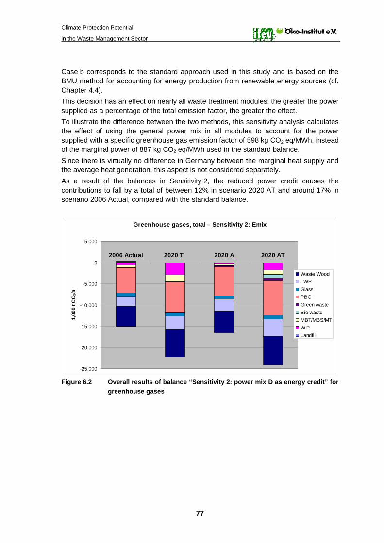
Climate Protection Potential
in the Waste Management Sector
77
Case b corresponds to the standard approach used in this study and is based on the BMU method for accounting for energy production from renewable energy sources (cf. Chapter 4.4). This decision has an effect on nearly all waste treatment modules: the greater the power supplied as a percentage of the total emission factor, the greater the effect. To illustrate the difference between the two methods, this sensitivity analysis calculates the effect of using the general power mix in all modules to account for the power supplied with a specific greenhouse gas emission factor of 598 kg CO2 eq/MWh, instead of the marginal power of 887 kg CO2 eq/MWh used in the standard balance. Since there is virtually no difference in Germany between the marginal heat supply and the average heat generation, this aspect is not considered separately. As a result of the balances in Sensitivity 2, the reduced power credit causes the contributions to fall by a total of between 12% in scenario 2020 AT and around 17% in scenario 2006 Actual, compared with the standard balance.
Greenhouse gases, total – Sensitivity 2: Emix
-25,000
-20,000
-15,000
-10,000
-5,000
0
5,000
1,00
0 t C
O2/a
Waste WoodLWPGlassPBCGreen wasteBio wasteMBT/MBS/MTWIPLandfill
2006 Actual 2020 T 2020 A 2020 AT
Figure 6.2 Overall results of balance “Sensitivity 2: power mix D as energy credit” for
greenhouse gases

Climate Protection Potential
in the Waste Management Sector
78
Table 6.3 Overall results of balance “Sensitivity 2: power mix D as energy credit” for greenhouse gases
2006
Actual 2020 T 2020 A 2020 AT
1,000 t
CO2 eq/a 1,000 t
CO2 eq/a 1,000 t
CO2 eq/a 1,000 t
CO2 eq/a Landfill 62 0 0 0 WIP -610 -2,916 -268 -1,754 M(B) plants -624 -1,512 -394 -1,040 Bio waste 104,3 -98 -30 -794 Green waste 85 -19 -332 -691 PBC -5,905 -7,141 -6,752 -8,164 Glass -897 -897 -897 -897 LWP -2,147 -3,183 -2,746 -4,112 Waste wood -4,860 -6,418 -5,107 -6,745 Total -14,790 -22,184 -16,526 -24,196
All figures except those for landfill and glass recycling are affected by this sensitivity.
In the balance “Sensitivity 2”, scenario 2020 AT with approx. 24,2 million t CO2 eq/a shows an increase of about 9,4 million t CO2 eq/a compared with the 2006 scenario. Table 6.4 shows the specific emission factors of the individual waste fractions for the case where the German power mix is taken as a basis for the credit. In the standard case this table corresponds to Table 5.5. Table 6.4 Specific greenhouse gas emission factors of the individual waste
treatment modules for greenhouse gases in the balance “Sensitivity 2: power mix D as energy credit” for greenhouse gases
2006
Actual 2020 T 2020 A 2020 AT
kg
CO2 eq/t kg
CO2 eq/t kg
CO2 eq/t kg
CO2 eq/t Landfill 664 0 0 0 WIP -56 -268 -34 -225 M(B) plants -86 -208 -75 -199 Bio waste 28 -26 -6 -151 Green waste 21 -5 -69 -144 PBC -731 -884 -731 -883 Glass -465 -465 -465 -465 LWP -474 -702 -469 -702 Waste wood -704 -930 -705 -931 Average -312 -468 -349 -511
All figures except those for landfill and glass recycling are affected by this sensitivity.
Figure 6.3 compares the balance results for this sensitivity with the results in the Status Report 2005. Since 2005 was also calculated using the power mix D, this is the closest approximation to the results obtained then.
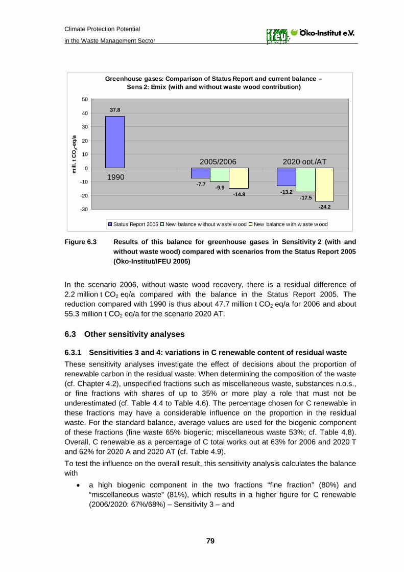
Climate Protection Potential
in the Waste Management Sector
79
Greenhouse gases: Comparison of Status Report and current balance – Sens 2: Emix (with and without waste wood contribution)
-13.2-7.7
37.8
-17.5
-9.9
-24.2
-14.8
-30
-20
-10
0
10
20
30
40
50
mill
. t C
O2-
eq/a
Status Report 2005 New balance w ithout w aste w ood New balance w ith w aste w ood
1990
2005/2006 2020 opt./AT
Figure 6.3 Results of this balance for greenhouse gases in Sensitivity 2 (with and
without waste wood) compared with scenarios from the Status Report 2005 (Öko-Institut/IFEU 2005) In the scenario 2006, without waste wood recovery, there is a residual difference of 2.2 million t CO2 eq/a compared with the balance in the Status Report 2005. The reduction compared with 1990 is thus about 47.7 million t CO2 eq/a for 2006 and about 55.3 million t CO2 eq/a for the scenario 2020 AT.
6.3 Other sensitivity analyses
6.3.1 Sensitivities 3 and 4: variations in C renewable content of residual waste These sensitivity analyses investigate the effect of decisions about the proportion of renewable carbon in the residual waste. When determining the composition of the waste (cf. Chapter 4.2), unspecified fractions such as miscellaneous waste, substances n.o.s., or fine fractions with shares of up to 35% or more play a role that must not be underestimated (cf. Table 4.4 to Table 4.6). The percentage chosen for C renewable in these fractions may have a considerable influence on the proportion in the residual waste. For the standard balance, average values are used for the biogenic component of these fractions (fine waste 65% biogenic; miscellaneous waste 53%; cf. Table 4.8). Overall, C renewable as a percentage of C total works out at 63% for 2006 and 2020 T and 62% for 2020 A and 2020 AT (cf. Table 4.9). To test the influence on the overall result, this sensitivity analysis calculates the balance with
• a high biogenic component in the two fractions “fine fraction” (80%) and “miscellaneous waste” (81%), which results in a higher figure for C renewable (2006/2020: 67%/68%) – Sensitivity 3 – and
Climate Protection Potential
in the Waste Management Sector
80
• a reduced biogenic component in the two fractions “fine fraction” (55%) and “miscellaneous waste” (10%)29
Since the proportion of unspecified waste fractions shows a marked rise after the increased removal of recyclables, an assumption that their content of renewable carbon is low results in a sizeable reduction in the biogenic component of the residual waste, whereas conversely an assumption that the content of renewable carbon is high increases the biogenic component.
, which results in a reduced figure for C renewable (2006/2020: 58%/54%) – Sensitivity 4.
The results of this sensitivity analysis have the greatest impact on waste incineration plants, for which they are set out in Chapter 4.4.2. The influence of this analysis on the overall result is shown in Chapter 6.4.
6.3.2 Sensitivity 5: Efficiency of waste incineration plants in line with Status Report 2005
Sensitivity analysis 5 investigates the effects that reduced efficiency of waste incineration plants in the scenarios 2020 T and 2020 AT has on the results for the waste incineration plants and the overall results. Power efficiency is raised from 14% to 15% compared with the standard balance, while heat efficiency is reduced from 45% to 36.8%. The results of this sensitivity analysis – Sens 5 – are set out for waste incineration plants in Chapter 4.4.2. The influence of this analysis on the overall result is shown in Chapter 6.4.
6.3.3 Sensitivities 6 and 7: Variation of efficiencies for substitute-fuel CHP plants
These sensitivity analyses investigate the effect of increasing the efficiency of substitute-fuel CHP plants. In Sensitivity 6, heat efficiency is raised from 40% to 60% while power efficiency remains unchanged. In Sensitivity 7, power efficiency is raised from 20% to 27%. The results of this sensitivity analysis have the greatest impact on M(B) plants, for which they are set out in Chapter 4.5.2. The influence of this analysis on the overall result is shown in Chapter 6.4.
6.3.4 Sensitivity 8: Variation in utilisation of sorting residues from bio and green waste treatment
This sensitivity analysis investigates the influence of optimised utilisation of sorting residues (treatment and partial recovery in substitute-fuel CHP plants) and additional screening out of a woody fraction (about 2.5% of the input) in the treatment of bio waste and green waste.
29 The high figures for the fine fraction and miscellaneous waste are in line with information from (IAA/INTECUS 2008), the low figures are from (Kern 2001).

Climate Protection Potential
in the Waste Management Sector
81
The results of this sensitivity analysis – Sens 8 – are set out for bio and green waste treatment in Chapter 4.6.6. The influence of this analysis on the overall result is shown in Chapter 6.4.
6.3.5 Sensitivity 9: Credit of power (fossil) mix and heat mix in Germany for utilisation of energy from the wood saved in PBC recycling
In Germany, the power (fossil) mix and heat mix to be credited for energy supplied is much higher than the figures used in the standard balance for average energy production in Sweden. This sensitivity analysis investigates the influence that utilisation of the wood in Germany, or as an approximation the delivery of the resulting electricity to Germany, has on the results for PBC recycling and on the overall result. The results of this sensitivity analysis – Sens 9 – are set out for PBC recycling in Chapter 4.7.2. The influence of this analysis on the overall result is shown in Chapter 6.4.
6.4 Comparison of standard balance and sensitivity analyses
As far as the overall results are concerned, only Sensitivities 1 and 9 display significant deviations from the standard balance (cf. Figure 6.4 and Table 6.5).
Greenhouse gases – Overall results, comparison of SB and sensitivities
-45
-40
-35
-30
-25
-20
-15
-10
-5
0
mill
. t C
O2-
eq/a
StandardSens 1Sens 2Sens 3Sens 4Sens 5Sens 6Sens 7Sens 8Sens 9
2006 Actual 2020 T 2020 A 2020 AT
Figure 6.4 Comparison of overall results for standard balance and sensitivities 1 to 9
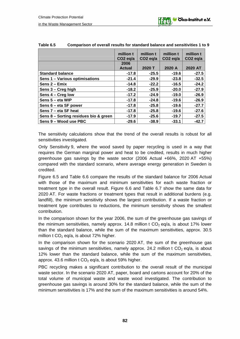
Climate Protection Potential
in the Waste Management Sector
82
Table 6.5 Comparison of overall results for standard balance and sensitivities 1 to 9
million t CO2 eq/a
million t CO2 eq/a
million t CO2 eq/a
million t CO2 eq/a
2006
Actual 2020 T 2020 A 2020 AT Standard balance -17.8 -25.5 -19.6 -27.5 Sens 1 – Various optimisations -21.4 -29.9 -23.8 -32.5 Sens 2 – Emix -14.8 -22.2 -16.5 -24.2 Sens 3 – Creg high -18.2 -25.9 -20.0 -27.9 Sens 4 – Creg low -17.2 -24.9 -19.0 -26.9 Sens 5 – eta WIP -17.8 -24.8 -19.6 -26.9 Sens 6 – eta SF power -17.8 -25.8 -19.6 -27.7 Sens 7 – eta SF heat -17.8 -25.8 -19.6 -27.6 Sens 8 – Sorting residues bio & green -17.9 -25.6 -19.7 -27.5 Sens 9 – Wood use PBC -29.6 -38.9 -33.1 -42.7
The sensitivity calculations show that the trend of the overall results is robust for all sensitivities investigated. Only Sensitivity 9, where the wood saved by paper recycling is used in a way that requires the German marginal power and heat to be credited, results in much higher greenhouse gas savings by the waste sector (2006 Actual +66%, 2020 AT +55%) compared with the standard scenario, where average energy generation in Sweden is credited. Figure 6.5 and Table 6.6 compare the results of the standard balance for 2006 Actual with those of the maximum and minimum sensitivities for each waste fraction or treatment type in the overall result. Figure 6.6 and Table 6.7 show the same data for 2020 AT. For waste fractions or treatment types that result in additional burdens (e.g. landfill), the minimum sensitivity shows the largest contribution. If a waste fraction or treatment type contributes to reductions, the minimum sensitivity shows the smallest contribution. In the comparison shown for the year 2006, the sum of the greenhouse gas savings of the minimum sensitivities, namely approx. 14.8 million t CO2 eq/a, is about 17% lower than the standard balance, while the sum of the maximum sensitivities, approx. 30.5 million t CO2 eq/a, is about 72% higher. In the comparison shown for the scenario 2020 AT, the sum of the greenhouse gas savings of the minimum sensitivities, namely approx. 24.2 million t CO2 eq/a, is about 12% lower than the standard balance, while the sum of the maximum sensitivities, approx. 43.6 million t CO2 eq/a, is about 59% higher. PBC recycling makes a significant contribution to the overall result of the municipal waste sector. In the scenario 2020 AT, paper, board and cartons account for 20% of the total volume of municipal waste and waste wood investigated. The contribution to greenhouse gas savings is around 30% for the standard balance, while the sum of the minimum sensitivities is 17% and the sum of the maximum sensitivities is around 54%.
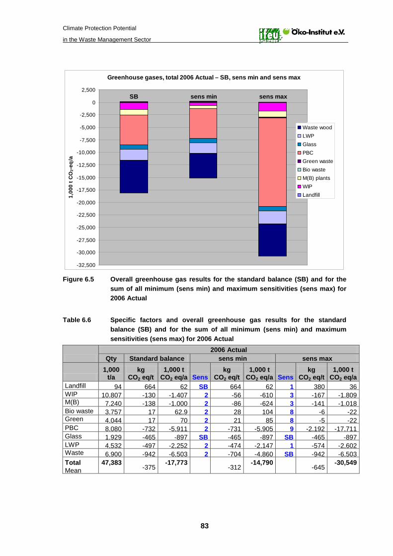
Climate Protection Potential
in the Waste Management Sector
83
Greenhouse gases, total 2006 Actual – SB, sens min and sens max
-32,500
-30,000
-27,500
-25,000
-22,500
-20,000
-17,500
-15,000
-12,500
-10,000
-7,500
-5,000
-2,500
0
2,500
1,00
0 t C
O2-
eq/a
Waste woodLWPGlassPBCGreen wasteBio wasteM(B) plantsWIPLandfill
SB sens min sens max
Figure 6.5 Overall greenhouse gas results for the standard balance (SB) and for the
sum of all minimum (sens min) and maximum sensitivities (sens max) for 2006 Actual
Table 6.6 Specific factors and overall greenhouse gas results for the standard
balance (SB) and for the sum of all minimum (sens min) and maximum sensitivities (sens max) for 2006 Actual
2006 Actual
Qty Standard balance sens min sens max
1,000
t/a kg
CO2 eq/t 1,000 t
CO2 eq/a Sens kg
CO2 eq/t 1,000 t
CO2 eq/a Sens kg
CO2 eq/t 1,000 t
CO2 eq/a Landfill 94 664 62 SB 664 62 1 380 36 WIP 10,807 -130 -1,407 2 -56 -610 3 -167 -1,809 M(B)
7,240 -138 -1,000 2 -86 -624 3 -141 -1,018
Bio waste 3,757 17 62,9 2 28 104 8 -6 -22 Green
4,044 17 70 2 21 85 8 -5 -22
PBC 8,080 -732 -5,911 2 -731 -5,905 9 -2,192 -17,711 Glass 1,929 -465 -897 SB -465 -897 SB -465 -897 LWP 4,532 -497 -2,252 2 -474 -2,147 1 -574 -2,602 Waste
6,900 -942 -6,503 2 -704 -4,860 SB -942 -6,503
Total Mean
47,383
-375 -17,773
-312
-14,790
-645 -30,549
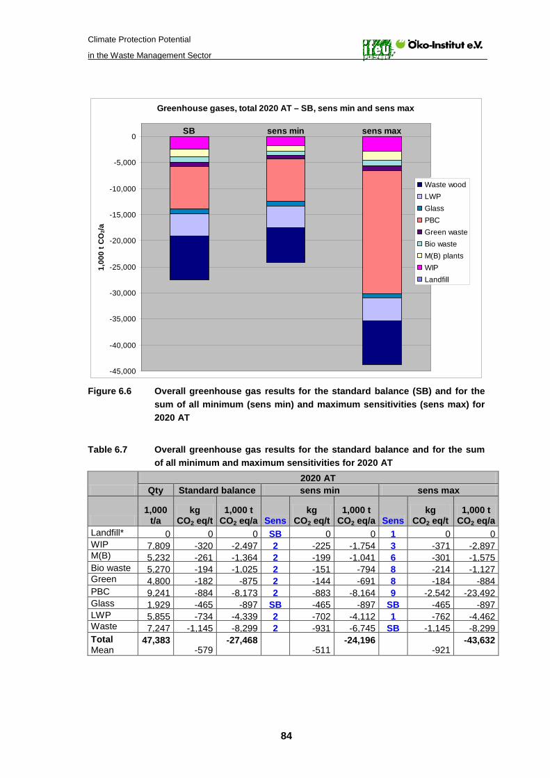
Climate Protection Potential
in the Waste Management Sector
84
Greenhouse gases, total 2020 AT – SB, sens min and sens max
-45,000
-40,000
-35,000
-30,000
-25,000
-20,000
-15,000
-10,000
-5,000
0
1,00
0 t C
O2/a
Waste woodLWPGlassPBCGreen wasteBio wasteM(B) plantsWIPLandfill
sens maxsens minSB
Figure 6.6 Overall greenhouse gas results for the standard balance (SB) and for the
sum of all minimum (sens min) and maximum sensitivities (sens max) for 2020 AT
Table 6.7 Overall greenhouse gas results for the standard balance and for the sum
of all minimum and maximum sensitivities for 2020 AT
2020 AT
Qty Standard balance sens min sens max
1,000
t/a kg
CO2 eq/t 1,000 t
CO2 eq/a Sens kg
CO2 eq/t 1,000 t
CO2 eq/a Sens kg
CO2 eq/t 1,000 t
CO2 eq/a Landfill* 0 0 0 SB 0 0 1 0 0 WIP 7,809 -320 -2,497 2 -225 -1,754 3 -371 -2,897 M(B)
5,232 -261 -1,364 2 -199 -1,041 6 -301 -1,575
Bio waste 5,270 -194 -1,025 2 -151 -794 8 -214 -1,127 Green
4,800 -182 -875 2 -144 -691 8 -184 -884
PBC 9,241 -884 -8,173 2 -883 -8,164 9 -2,542 -23,492 Glass 1,929 -465 -897 SB -465 -897 SB -465 -897 LWP 5,855 -734 -4,339 2 -702 -4,112 1 -762 -4,462 Waste
7,247 -1,145 -8,299 2 -931 -6,745 SB -1,145 -8,299
Total Mean
47,383 -579
-27,468 -511
-24,196 -921
-43,632
Climate Protection Potential
in the Waste Management Sector
85
7 Evaluation of balance results
Under the Kyoto Protocol, the EU (EU 15) undertook to make an 8% reduction in greenhouse gas emissions by 2012 compared with the base year 199030
The National Inventory Report (NIR) (UBA 2009) shows that during the same period the emissions reported in the “Waste” sector (consisting largely of waste deposition as landfill and wastewater treatment) fell from 40.4 to 12.3 million t CO2 eq/a. Thus the national reporting also shows that the waste sector’s contribution up to 2006, with a drop of around 70%, was well above the percentage decrease in total emissions.
. In order to achieve this target, Germany promised under the EU burden-sharing agreement to reduce its national emissions by 21%. According to the latest National Inventory Report for Germany (UBA 2009), total emissions in 2006 (excluding Land Use, Land Use Change and Forestry – LULUCF) came to 981 million t CO2 eq. Compared with the total burden of 1,215 million t CO2 eq in the base year 1990 this corresponds to a reduction of 235 million t CO2 eq/a or 19%. This means that the above mentioned reduction target for 2012 had already been nearly met in 2006.
The goal of tracking compliance with the national contributions to the Kyoto Protocol means it is not necessary, and is in fact virtually impossible, to give a precise representation of the contributions made by the individual segments. For this reason the most important climate-relevant emissions are reported under the heading “Waste”, for example methane emissions from landfill, methane and nitrous oxide emissions from biological treatment (including MBT), and nitrous oxide and methane emissions from wastewater treatment. The benefits achieved by the waste sector, such as substitution of primary raw materials by recycling or energy generation from waste incineration, are not found under the heading “Waste”, but make themselves felt in the sectors where they are saved. For the substitution of primary raw materials this is the “Industrial Processes” sector, where the greenhouse gas emissions which would have been caused by the substituted primary product are now replaced by the emissions due to the recycling product produced. Generation of energy from waste is reported under the “Energy” sector, and this logically applies to emissions from combustion of waste in incineration plants if this is used to generate energy.
0102030405060708090
1. Qrtl. 2. Qrtl. 3. Qrtl. 4. Qrtl.
OstWestNord
30 For the parameters HFC, PFC and SF6 the base year is 1995

Climate Protection Potential
in the Waste Management Sector
86
Figure 7.1 Emissions in Germany since 1990, by source categories (UBA 2009)
For a comprehensive evaluation of the overall contribution of an industry or sector, the life cycle assessment approach is more suitable. It was therefore chosen in the Status Report 2005 and is chosen in this study to present an overall balance of the waste sector’s contribution to climate protection. There are thus considerable limitations on the extent to which the overall emissions and the reductions achieved or targeted as shown by national reporting can be compared with the results of this balance and climate balances with a life cycle assessment approach. In life cycle assessments and climate balances for the waste sector, a comprehensive description of waste sector performance in the field of recycling and thermal utilisation is therefore achieved by “crediting” the waste sector with emissions saved by reduced primary production or by reduced energy generation with primary fuels. These credits include all upstream chains (cf. Chapter 3). By contrast, as described above, the emissions reported in the NIR are allocated to the individual sectors in which they directly occur. The resulting restrictions on comparability of the results obtained using the different methodological approaches must be borne in mind in the following comparisons and assessments. The fall of 49.1 million t CO2 eq/a31
31 Bearing in mind the limited comparability of this study with the Status Report 2005, from which the figure for 1990 is taken (cf.
or 130% shown in this study from 1990 to 2006 for the waste sector excluding waste wood accounts for about 21% of the drop of 235 million t CO2 eq in 2006 compared with 1990 which is reported in the NIR. Including
Figure 5.4)

Climate Protection Potential
in the Waste Management Sector
87
waste wood recycling32
Table 7.1, the fall from 1990 to 2006 rises to 55.6 million t CO2 eq/a or
147% (cf. ) and accounts for 24% of the total drop shown by national reporting. Table 7.1 Overall greenhouse gas emissions and share due to waste sector in
Germany 1990 and 2006, plus savings achieved according to NIR (UBA 2009) and this study
1990 2006 Reduction
mill. t/a mill. t/a mill. t/a % Total emissions NIR without LULUCF* 1,215 981 235 19 Waste sector acc. to NIR 40.4 12.3 28.1 70 Waste sector LCA approach excl. waste wood 37.8 -11.3 49.1 130 Waste sector LCA approach incl. waste wood 37.8 -17.8 55.6 147 Table 7.2 Greenhouse gas emissions and share due to waste sector in Germany
1990 and 2006, plus annual savings achieved per head of population according to NIR and this study
1990 2006 Reduction
t/(head*a) t/(head*a) t/(head*a) % Total emissions NIR without LULUCF 15 12 2.8 19 Waste sector acc. to NIR 0.49 0.15 0.34 70 Waste sector LCA approach excl. waste wood 0.46 -0.14 0.60 130 Waste sector LCA approach incl. waste wood 0.46 -0.22 0.67 147
Based on a population of 82.4 million
Table 7.2 shows that on an overall calculation based on the life cycle assessment approach, the optimised waste sector contributed some 600 kg CO2 eq/(head*a) of the total saving of 2.8 t CO2 eq/(head*a) which national reporting indicates was achieved in 2006 compared with 1990 (taking the results of this study for 2006 excluding waste wood). Using the figure including waste wood33
Germany is seeking to reduce total emissions by 40% by 2020. Compared with 1990 this would, according to national reporting, correspond to 486 million t CO2 eq/a. For comparison: the scenario 2020 AT investigated in this study, excluding waste wood, would save 57 million t CO2 eq/a compared with 1990 (according to Status Report 2005). This would amount to the waste sector making a contribution of 11.7% to the savings target for Germany. If waste wood utilisation is included, the greenhouse gas saving by the waste sector increases to 65.3 million t CO2 eq/a in 2020 compared with 1990, and the possible contribution to the national target increases to 13.4%.
increases the contribution to 670 kg CO2 eq/(head*a).
On the basis of a population of 82.4 million, the 40% reduction target for Germany corresponds to a saving of around 5.9 t CO2 eq/(head*a) of the population of Germany. According to this study, the waste sector’s possible contribution is around 690 kg
32 Waste wood was not investigated in the balance for 1990. 33 Cf. footnote 32.

Climate Protection Potential
in the Waste Management Sector
88
CO2 eq/(head*a) without waste wood, or about 790 kg per head per year with waste wood.

Climate Protection Potential
in the Waste Management Sector
89
8 Looking at the EU 27
The calculations for the EU 27 are performed solely for “Municipal Solid Waste” (MSW), i.e. the quantities of municipal waste that are reported to EUROSTAT by the Member States. For the EU 27 this also applies to waste wood, i.e. only quantities from the municipal sector are taken into account. Thus the results inevitably differ from the results in (Prognos/IFEU/INFU 2008), which looks at the total waste potential of all source sectors. Since municipal waste, although a very important part, is not the largest part of the waste management sector, the overall climate protection contribution made by the waste sector, to which the industrial and construction sectors contribute relevant quantities of waste, is considerably larger.
8.1 Waste quantities EU 27
The EUROSTAT data for 2007 are now available for the EU 27 and all Member States with regard to total quantities of municipal waste and the components deposited as landfill, incinerated, recycled (dry recyclables) and composted (with no distinction as to type of waste or composting method). As the relevant data for 2006 are less detailed, the figures for 2007 are used in the balance for the EU 27.

Climate Protection Potential
in the Waste Management Sector
90
Table 8.1 Waste quantities for EU 27 in 2007 (EUROSTAT 2009)
Total Landfill WIP Recycling Compost Residual 1,000 t/a 1,000 t/a 1,000 t/a 1,000 t/a 1,000 t/a 1,000 t/a EU27 258,199 105,785 51,286 55,017 42,012 4,098 EU15 220,201 76,546 50,302 53,052 41,423 -1,122 Austria AT 4,951 712 1,497 1,143 2,016 -417 Belgium BE 5,211 224 1,712 1,964 1,153 158 Bulgaria BG 3,593 2,980 0 0 0 613 Cyprus CY 587 512 0 75 0 0,00 Czech Rep. CZ 3,025 2,498 375 54 34 63 Denmark DK 4,364 224 2,324 1,064 763 -11 Estonia EE 719 390 1 205 10 113 Finland FI 2,675 1,411 310 695 258 0 France FR 34,309 11,750 12,321 5,381 4,857 0 Germany DE 46,448 271 15,803 20,830 8,010 1,534 Greece EL 5,002 4,148 0 756 98 0 Hungary HU 4,594 3,429 382 490 64 228 Ireland IE 3,398 2,015 0 1,081 79 223 Italy IT 32,548 16,912 3,955 4,063 12,171 -4,553 Latvia LV 861 735 3 106 5 11 Lithuania LT 1,354 1,245 0 29 22 57 Luxembourg LU 331 62 117 1 71 80 Malta MT 266 247 0 6 12 0 Netherlands NL 10,308 224 3,268 2,760 2,384 1,672 Poland PL 12,264 9,098 41 580 363 2,181 Portugal PT 5,007 3,150 968 400 490 0 Romania RO 8,183 6,122 0 34 2 2,024 Slovak. Rep. SK 1,669 1,295 180 28 76 90 Slovenia SI 886 688 0 357 0 -160 Spain ES 26,154 15,569 2,591 3,496 4,498 0 Sweden SE 4,717 189 2,191 1,738 561 38 United Kingdom UK 34,780 19,685 3,245 7,680 4,016 154
EU 15 countries marked in blue

Climate Protection Potential
in the Waste Management Sector
91
Table 8.2 Specific waste quantities for EU 27 in 2007 (EUROSTAT 2009)
Total Landfill WIP Recycling Compost Residual
kg/(head*a) kg/(head*a) kg/(head*a) kg/(head*a) kg/(head*a) kg/(head*a) EU27 522 214 104 111 85 8 EU15 562 195 128 135 106 -3 Austria AT 597 86 180 138 243 -50 Belgium BE 492 21 162 186 109 15 Bulgaria BG 468 388 0 0 0 80 Cyprus CY 754 658 0 96 0 0.00 Czech Rep. CZ 294 243 36 5 3 6 Denmark DK 801 41 427 195 140 -2 Estonia EE 536 291 1 153 8 84 Finland FI 507 267 59 132 49 0 France FR 541 185 194 85 77 0 Germany DE 564 3 192 253 97 19 Greece EL 448 371 0 68 9 0 Hungary HU 456 341 38 49 6 23 Ireland IE 788 467 0 251 18 52 Italy IT 550 286 67 69 206 -77 Latvia LV 377 322 2 47 2 5 Lithuania LT 400 368 0 9 7 17 Luxembourg LU 694 130 245 3 149 167 Malta MT 652 606 0 15 30 0 Netherlands NL 630 14 200 169 146 102 Poland PL 322 239 1 15 10 57 Portugal PT 472 297 91 38 46 0 Romania RO 379 284 0 2 0 94 Slovak. Rep. SK 309 240 33 5 14 17 Slovenia SI 441 342 0 178 0 -79 Spain ES 588 350 58 79 101 0 Sweden SE 518 21 240 191 62 4 United Kingdom UK 572 324 53 126 69
EU 15 countries marked in blue
With regard to the quantities recycled and composted, EUROSTAT has no further information as to what types of waste are involved. At least for the composted quantities there is another source (ORBIT/ECN 2008) which can be used for a breakdown by country. The relevant figures are shown in Table 8.3. The information in ORBIT/ECN (2008) on separately collected bio waste in the EU and the information for the individual countries on quantities composted from bio waste, green waste, sewage sludge and household waste has been used to estimate, on the basis of the composted quantities reported to EUROSTAT, the bio waste quantities that can be assumed to be collected separately and sent for bio waste or green waste composting.

Climate Protection Potential
in the Waste Management Sector
92
Table 8.3 Composted quantities by waste type (EUROSTAT 2009), (ORBIT/ECN 2008), (own estimate)
Compost
Separately collected organic
Composted bio waste (estim.)
Composted household waste (estim.)
Composted sewage sludge (estim.)
EUROSTAT ORBIT/ECN 1,000 t/a 1,000 t/a 1,000 t/a 1,000 t/a 1,000 t/a EU27 42,012 23,599 32,386 5,170 4,457 EU15 41,423 23,196 31,806 5,170 4,447 Austria AT 2,016 1,496 1,902 13 102 Belgium BE 1,153 885 1,153 0 0 Bulgaria BG 0 0 0 0 0 Cyprus CY 0 0 0 0 0 Czech Rep. CZ 34 133 34 0 0 Denmark DK 763 775 763 0 0 Estonia EE 10 0 10 0 0 Finland FI 258 450 215 0 43 France FR 4,857 2,700 2,126 1,170 1,560 Germany DE 8,010 8,338 8,010 0 0 Greece EL 98 2 9 88 0 Hungary HU 64 127 64 0 0 Ireland IE 79 123 79 0 0 Italy IT 12,171 2,430 10,447 0 1,724 Latvia LV 5 0 5 0 0 Lithuania LT 22 0 22 0 0 Luxembourg LU 71 52 71 0 0 Malta MT 12 0 12 0 0 Netherlands NL 2,384 3,356 2,384 0 0 Poland PL 363 70 363 0 0 Portugal PT 490 34 63 385 41 Romania RO 2 0 2 0 0 Slovak. Rep. SK 76 73 67 0 9 Slovenia SI 0 0 0 0 0 Spain ES 4,498 308 184 3,367 947 Sweden SE 561 375 503 58 0 United Kingdom UK 4,016 1,872 3,898 89 30
EU 15 countries marked in blue
This study also examines the quantities of household waste that are composted. Household waste composting is still very common in France, Spain and Portugal. Unlike the composted quantities, there are no data on the recycled quantities with a similar degree of accuracy and detail for the individual countries. On the basis of the Prognos (2008) findings, estimates have been made of how the total recycling quantities reported to EUROSTAT break down into waste fractions for the EU 27. The Prognos (2008) figures were updated on the basis of a personal communication (Prognos 2009), and the relevant figures can be seen in Table 8.4. This table first lists the overall potentials and recycled quantities (energy and material) of recyclable waste – from
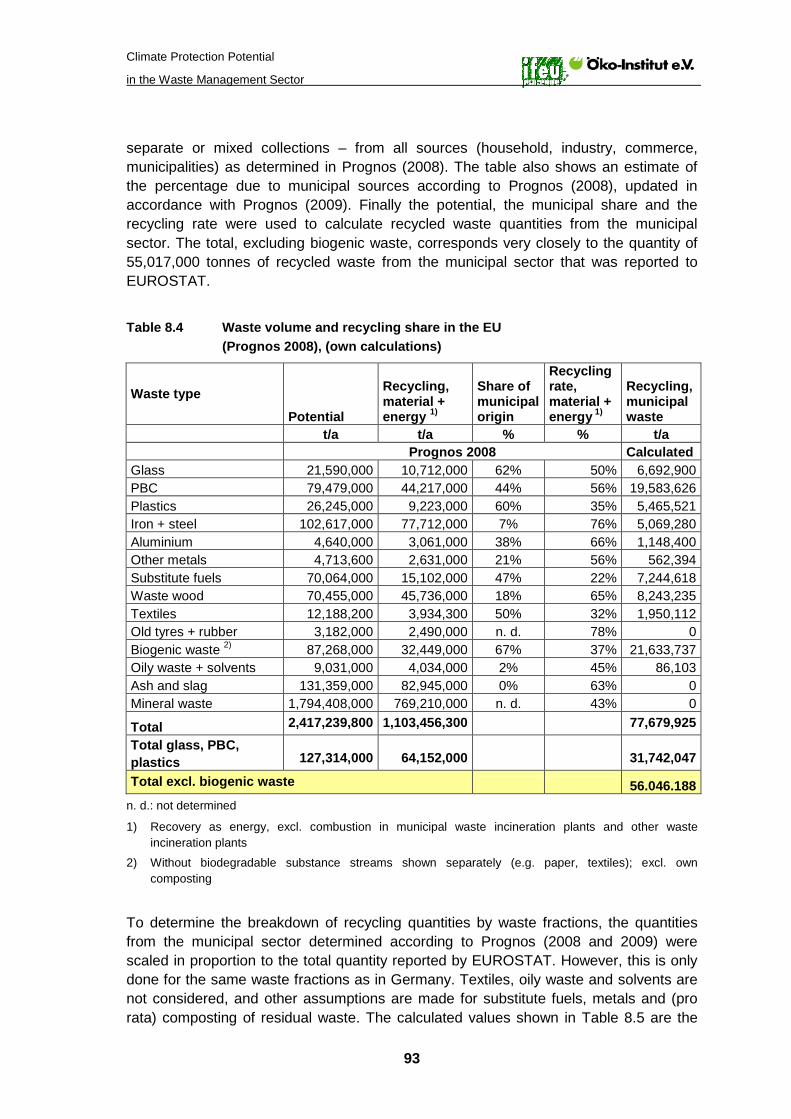
Climate Protection Potential
in the Waste Management Sector
93
separate or mixed collections – from all sources (household, industry, commerce, municipalities) as determined in Prognos (2008). The table also shows an estimate of the percentage due to municipal sources according to Prognos (2008), updated in accordance with Prognos (2009). Finally the potential, the municipal share and the recycling rate were used to calculate recycled waste quantities from the municipal sector. The total, excluding biogenic waste, corresponds very closely to the quantity of 55,017,000 tonnes of recycled waste from the municipal sector that was reported to EUROSTAT. Table 8.4 Waste volume and recycling share in the EU
(Prognos 2008), (own calculations)
Waste type Potential
Recycling, material + energy 1)
Share of municipal origin
Recycling rate, material + energy 1)
Recycling, municipal waste
t/a t/a % % t/a Prognos 2008 Calculated Glass 21,590,000 10,712,000 62% 50% 6,692,900 PBC 79,479,000 44,217,000 44% 56% 19,583,626 Plastics 26,245,000 9,223,000 60% 35% 5,465,521 Iron + steel 102,617,000 77,712,000 7% 76% 5,069,280 Aluminium 4,640,000 3,061,000 38% 66% 1,148,400 Other metals 4,713,600 2,631,000 21% 56% 562,394 Substitute fuels 70,064,000 15,102,000 47% 22% 7,244,618 Waste wood 70,455,000 45,736,000 18% 65% 8,243,235 Textiles 12,188,200 3,934,300 50% 32% 1,950,112 Old tyres + rubber 3,182,000 2,490,000 n. d. 78% 0 Biogenic waste 2) 87,268,000 32,449,000 67% 37% 21,633,737 Oily waste + solvents 9,031,000 4,034,000 2% 45% 86,103 Ash and slag 131,359,000 82,945,000 0% 63% 0 Mineral waste 1,794,408,000 769,210,000 n. d. 43% 0
Total 2,417,239,800 1,103,456,300 77,679,925 Total glass, PBC, plastics 127,314,000 64,152,000 31,742,047
Total excl. biogenic waste 56.046.188 n. d.: not determined
1) Recovery as energy, excl. combustion in municipal waste incineration plants and other waste incineration plants
2) Without biodegradable substance streams shown separately (e.g. paper, textiles); excl. own composting
To determine the breakdown of recycling quantities by waste fractions, the quantities from the municipal sector determined according to Prognos (2008 and 2009) were scaled in proportion to the total quantity reported by EUROSTAT. However, this is only done for the same waste fractions as in Germany. Textiles, oily waste and solvents are not considered, and other assumptions are made for substitute fuels, metals and (pro rata) composting of residual waste. The calculated values shown in Table 8.5 are the

Climate Protection Potential
in the Waste Management Sector
94
result of these assumptions. These figures are taken as a basis for the scenario 2007 Actual. The EUROSTAT figures for landfill and incineration were adopted as such. In addition to the waste fractions mentioned above which were not included, this section also disregards sewage sludge composting and the residual quantities for which EUROSTAT has no information about what happens to them. Composting of MSW is subdivided into bio and green waste composting derived from ORBIT/ECN (2008), and a proportion of residual waste composting (calculated from 1.36 million t of residual waste compost according to (ORBIT/ECN 2008)). It is assumed that the remaining difference goes for treatment in M(B) plants. For the recycling quantity, the recalculated figures for glass, paper, plastics and waste wood are adopted directly as values for calculation. For the relatively large quantities of iron + steel, aluminium, other metals and substitute fuels, by contrast, the situation has been simplified by estimating an input quantity into M(B) plants which represents the latter in the calculations. Table 8.5 Waste quantities in the EU 27 in 2007, derived figures based on Prognos
(2008 and 2009) and figures used for calculation
EUROSTAT Derived figures Calculated figures
t/a t/a t/a Municipal waste, landfill 105,785,285 105,785,285 105,785,285 Municipal waste, WIP 51,286,132 51,286,132 51,286,132 Municipal waste, composting 42,012,432 Composting of separately collected bio waste 32,385,981 32,385,981
Refuse composting 5,169,827 2,721,370 Sewage sludge comp. (not considered) 4,456,624 Municipal waste, recycling 55,017,271 Glass 6,570,029 6,570,029 PBC 19,224,102 19,224,102 Plastics 5,365,183 5,365,183 Iron + steel 4,976,216 Aluminium 1,127,317 Other metals 552,069 SF 7,111,618 Input M(B) plants 17,779,046 Waste wood 8,091,903 8,091,903 Textiles (not considered) 1,914,311 Oily waste + solvents (not considered) 84,522 Remainder (not considered) 4,098,202 4,098,202 1)
Total municipal waste 258,199,323 258,199,323 249,209,032 1) The total of the quantities derived as calculation figures diverges from the overall Eurostat total by 8,990,291 t/a.
In the case of waste wood, a different approach than for Germany is adopted when considering the EU 27. Instead of the total volume in the EU 27, only the municipal sector is examined here in the form of the calculated 8 million tonnes, as for all other waste fractions. Although it is basically possible, according to (EC 2009), to include the entire volume of waste wood in the balance in the same way as for Germany, this total
Climate Protection Potential
in the Waste Management Sector
95
quantity (as Table 8.6 shows) is very high by comparison with the other waste fractions investigated, which means the waste wood potential would play a very dominant role in the results. Moreover, the waste wood potential according to (EC 2009) is in particular dominated by the item “Packaging wood, sawdust, wood chips etc.” and hence by commercial waste, which must not be included in the figures for Germany because these quantities are often used directly or within the company. Table 8.6 Waste wood potential in the EU 27 according to (EC 2009) Source sector Volume [t/a] Municipal waste or bulky waste 8,225,000 Packaging wood, sawdust, wood chips etc. 45,718,000 Construction and demolition wood 9,757,000 Production sector 6,715,000 End-of-life vehicles 40,000 Total 70,455,000
8.2 Scenarios EU 27
A total of three scenarios were defined for the EU 27: one “Actual” scenario with the waste quantities derived above (2007) and two separate future scenarios 2020 I and 2020 II. Calculation of credits and debits is largely on the basis of the emission factors determined for Germany. This also means that no adjustment is made to power consumption, i.e. the German power mix is retained. This simplification produces only a slight discrepancy in the result, since the difference for greenhouse gases at 541 g CO2 eq/kWhel in the EU 27 mix instead of 598 g CO2 eq/kWhel for Germany is negligible. Conversely, however, the power credit, instead of the marginal power figure for Germany (887 g CO2 eq/kWhel), uses a substitution mix of 50% coal and 50% natural gas for the EU 27, which works out at 749 g CO2 eq/kWhel. Further exceptions concern individual treatment processes, for which more information was available or for which plausible assumptions could be made. These are described in Chapter 8.3. • 2007 (Actual)
Life cycle assessment of actual situation in accordance with the data from Eurostat, supplemented by own calculations; credits and debits for products and energy consumed or supplied are based, with a few exceptions (Chapter 8.3) on the data for Germany.
• 2020 I Assumes that landfill will be discontinued and that the quantities hitherto sent for landfill will, with the exception of waste wood, be divided among the waste fractions (bio and green waste, glass, PBC, plastics) and disposal paths (incineration, M(B) plants), weighted on the basis of their share of the Actual situation. For waste wood it is assumed that the recycling rate will increase from the current 65% to 90%. It is also assumed that refuse composting34
34 Here “refuse composting” is taken to mean composting of household waste not separately collected, with the resulting refuse compost being used largely in agriculture and forestry. By
will be

Climate Protection Potential
in the Waste Management Sector
96
discontinued and – for the sake of simplicity – that the relatively small quantity will be added to the bio waste quantity. Implementing these assumptions would mean that a total of 47% of waste would be recycled in the scenario 2020 I. This almost meets the requirements of the Framework Directive on Waste, under which at least 50% is to be recycled by 2020.
• 2020 II Assumes that landfill will be discontinued, and that the quantities hitherto sent for landfill will now be redistributed as in the situation assumed for Germany in the scenario 2020 T. This is essentially the Actual situation in Germany in 2006, except that there is definitely no longer any direct deposition of waste as landfill. Again the waste wood quantity is an exception. Here it is assumed, as in scenario 2020 I, that the recycling rate increases from 65% to 90%. Unlike the German situation, it is not assumed that a “Dual System” will become established in the EU 27. Instead, the quantity corresponding to LWP in Germany is modelled as plastics, composites and metal packaging, and is summarised under “Plastics and packaging waste” in Table 4.31.
Table 8.7 shows the resulting quantities in the three scenarios. Table 8.7 Waste streams in the scenarios for the EU 27 2007 Actual 2020 I 2020 II 1,000 t/a % 1,000 t/a % 1,000 t/a % Landfill 105,785 42.4% 0 0% 0 0% WIP 51,286 20.6% 90,196 36.2% 63,866 25.6% M(B) plants 17,779 7.1% 31,268 12.5% 42,788 17.2% Refuse composting 2,721 1.1% 0 0% 0 0% Bio waste (bio bin) 14,898 6.0% 30,986 12.4% 22,088 8.9% Green waste (total) 17,488 7.0% 30,756 12.3% 23,775 9.5% PBC 19,224 7.7% 33,809 13.6% 47,503 19.1% Glass 6,570 2.6% 11,555 4.6% 11,341 4.6% Plastics + packaging waste 5,365 2.2% 9,436 3.8% 26,644 10.7% Waste wood 8,092 3.2% 11,204 4.5% 11,204 4.5% Total 249,209 100.0% 249,209 100.0% 249,209 100.0%
8.3 Waste treatment EU 27
As already mentioned, the calculation of the EU 27 scenarios largely follows the basic data for Germany (input, emissions, waste composition). This is the case in scenario 2007 Actual for residual waste treatment in waste incineration plants and M(B) plants, and for PBC, glass, waste wood and green waste recovery. Consequently, glass recovery – as in Germany – is not subject to technical changes. Unlike in the German contrast, biological treatment of residual waste in M(B) plants, with landfill of the rotted residues and creation and use of compost from separately collected bio waste meeting quality criteria defined under legal (Bio Waste Ordinance) or voluntary (BGK) requirements, is a promotable alternative to such refuse composting.

Climate Protection Potential
in the Waste Management Sector
97
balance, for waste wood an individual split is used for the components recovered as energy and material. According to (Prognos 2008), 47% of the recycled waste wood is recovered as material and 53% as energy. Since, as in the balance for Germany, a credit is given not only for recovery as material, but also for utilisation of the saved wood as energy, the shift in the split between material and energy utilisation produces only a slight difference in the emission factor for waste wood. Changes in the future scenarios for waste wood and waste paper arise solely from the improvements in efficiency (wood-burning CHP plants). For the scenarios for 2020, the emission factors of scenario 2020 T for Germany were used, except for bio and green waste, which means that the associated technical optimisations, in particular, were also assumed for EU 27. This also applies in principle to waste incineration plants (cf. Chapter 4.4) and M(B) plants (cf. Chapter 4.5) , though for waste incineration plants a less optimistic heat efficiency level is assumed (including for utilisation of substitute fuels from M(B) plants) in the 2020 scenarios (35% instead of 45%). Treatment in M(B) plants benefits from improvements, likewise as a result of efficiency optimisation in the substitute-fuel power plants and wood-burning CHP plants. For utilisation of green waste, the technical optimisations and the division of substance streams are assumed to be similar to the situation in Germany (18.75% woody component for energy use in wood-burning CHP plants and 18.75% for combined material and energy utilisation in fermentation plants) and the emission factors of scenario 2020 AT are used accordingly. Further assumptions about waste treatment are described in more detail below.
8.3.1 Landfill The modelling of landfill for the scenario 2007 Actual is also based on the IPCC (1996) requirements. Unlike the situation in Germany, however, it cannot be assumed that all landfill sites have a gas capture facility. It is basically assumed for the EU 27 that about 40% of landfill sites are equipped with a gas capture facility. Given a mean effective gas capture potential of about 50%, this works out at a mean effective gas capture rate of 20% for the EU 27. Experience in other studies shows (ETC 2009) that the gas capture rate is the subject of controversy at EU level. Individual Member States such as the UK claim that they achieve a much higher effective gas capture rate of up to 80%. Although the authors take the view that such a high gas capture rate is not technically plausible, especially in view of the filling phase of a landfill site, they nevertheless cater for the divergent opinions in the EU by including an effective gas capture rate of 40% as well as the 20% rate mentioned above. The results show variants with and without carbon storage (C-sink). Here C-sink means the organic carbon component in the waste that is not degraded and converted into landfill gas, but remains for a long period in the landfill site. Although this amount is quantifiable, it is not included in the greenhouse gas inventory under IPCC (1996, 2006). Including the C-sink as standard for landfill sites is problematical in that this would only be correct if the C-sink were taken into account in all other possible areas, e.g. in furniture or books as well. Such comprehensive inclusion of the C-sink is not feasible, however. For landfill sites it is therefore shown as a sensitivity analysis.
Climate Protection Potential
in the Waste Management Sector
98
8.3.2 Plastics and packaging waste For plastics and packaging waste (cans, composites) it is assumed that “take systems” will tend to predominate. On the one hand this will probably result in a smaller proportion of the total potential being achieved, but on the other it will probably reduce the proportion of sorting residues resulting from sorting errors. Unlike the German LWP system, the sorting residue component is assumed to be 20% (Germany approx. 40% in 2006, Table 4.31) and, also unlike the German system, this is all allocated to thermal treatment in waste incineration plants. It is also assumed that plastics can largely be recycled as homogeneous plastic fractions (films, bottles, tubs, PET), without any appreciable quantities of mixed plastics occurring. The further recovery of plastic fractions and packaging waste is assumed to be in line with the data for Germany.
8.3.3 Refuse composting Refuse composting, which is common in France, Spain and Portugal in particular, is accounted for without any benefit. As a rule the resulting refuse compost products contain high levels of pollutants and should not be used for high-quality applications. It is assumed that they are only suitable for use in recultivation situations, e.g. on landfill sites. The input for refuse composting is derived from green waste composting (largely open systems and use of diesel-powered units).
8.3.4 Bio waste recovery In the case of bio waste recovery the German actual data for operating expenditure and emissions are largely retained. On average, the uses to which the compost is put show only slight differences from the German situation, as can be seen in Table 8.8. Therefore, as in the German balance, the data according to (BGK 2008) are used. Unlike the German situation, however, a smaller share is assumed for fermentation, with 10% instead of 15%. For the scenarios for 2020, the same technical optimisations and optimisations in the steering of substance streams as for Germany were also assumed for EU27 (Chapter 4.6), as in the case of green waste. Here too, the only exception is the share for fermentation, which is assumed to rise to 50% instead of to 80%. Table 8.8 Uses of compost in Germany and the EU
Anaerobic compost Germany
Aerobic compost Germany
Aerobic compost EU
IFEU (2001) BGK (2008) ORBIT/ECN (2008) % % % Agriculture 73 52 56 Fruit growing 1 6 Market gardening 1 7 11 Earthworks 4 11 6 GaLa + municipal 13 12 10 Private gardening 1 11 12 Recultivation 6 2 5
GaLa: Horticulture and Landscape Gardening
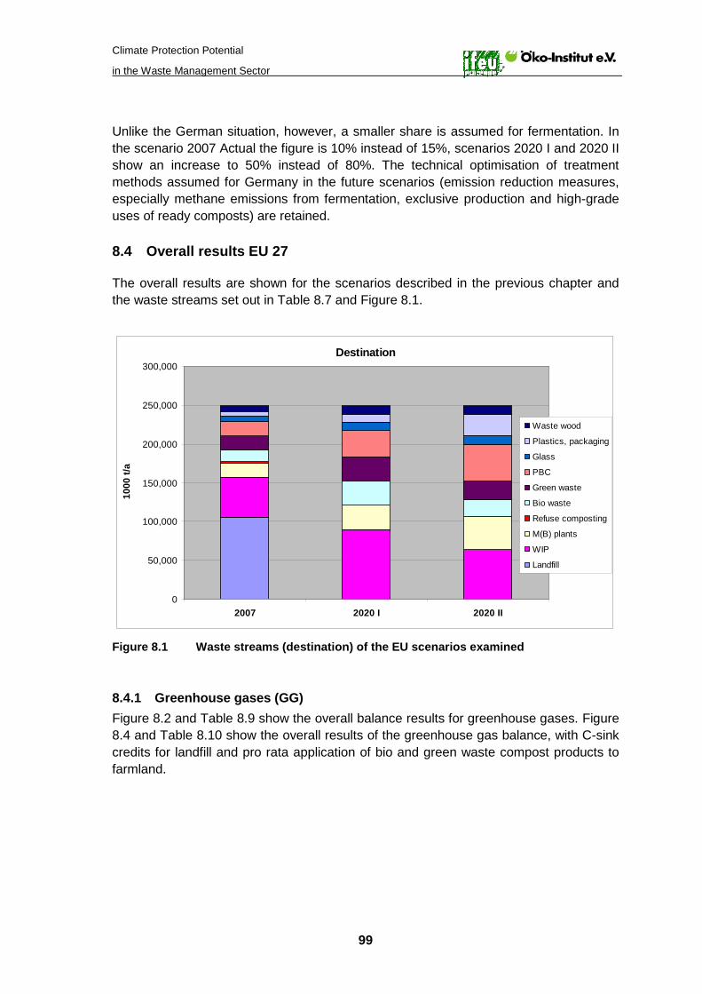
Climate Protection Potential
in the Waste Management Sector
99
Unlike the German situation, however, a smaller share is assumed for fermentation. In the scenario 2007 Actual the figure is 10% instead of 15%, scenarios 2020 I and 2020 II show an increase to 50% instead of 80%. The technical optimisation of treatment methods assumed for Germany in the future scenarios (emission reduction measures, especially methane emissions from fermentation, exclusive production and high-grade uses of ready composts) are retained.
8.4 Overall results EU 27
The overall results are shown for the scenarios described in the previous chapter and the waste streams set out in Table 8.7 and Figure 8.1.
Destination
0
50,000
100,000
150,000
200,000
250,000
300,000
2007 2020 I 2020 II
1000
t/a
Waste wood
Plastics, packaging
Glass
PBC
Green waste
Bio waste
Refuse composting
M(B) plants
WIP
Landfill
Figure 8.1 Waste streams (destination) of the EU scenarios examined
8.4.1 Greenhouse gases (GG) Figure 8.2 and Table 8.9 show the overall balance results for greenhouse gases. Figure 8.4 and Table 8.10 show the overall results of the greenhouse gas balance, with C-sink credits for landfill and pro rata application of bio and green waste compost products to farmland.

Climate Protection Potential
in the Waste Management Sector
100
Greenhouse gases, total
-150,000
-100,000
-50,000
0
50,000
100,000
150,000
2007 2020 I 2020 II
1.00
0 t C
O2
eq/a
Waste woodPlastics, packagingGlassPBCGreen wasteBio wasteRefuse compostingM(B) plantsWIPLandfillLandfill
40% eff. gas capture
20% eff. gas capture
Figure 8.2 Overall results of standard balance EU 27 for greenhouse gases Table 8.9 Overall results of standard balance EU 27 for greenhouse gases 2007 2020 I 2020 II 1,000 t CO2 eq/a 1,000 t CO2 eq/a 1,000 t CO2 eq/a Landfill 20% eff. 109,930 0 0 Landfill 40% eff. 83,112 0 0 WIP -4,864 -21,374 -15,135 M(B) plants -2,012 -7,080 -9,688 Refuse composting 204 0 0 Bio waste 386 -3,214 -2,291 Green waste 333 -4,942 -3,820 PBC -14,056 -29,870 -41,968 Glass -3,054 -5,371 -5,271 Plastics, packaging -2,233 -6,936 -24,636 Waste wood -6,665 -11,608 -11,608 Total (landfill 20%) 77,970 -90,395 -114,418 Total (landfill 40%) 51,152 -90,395 -114,418

Climate Protection Potential
in the Waste Management Sector
101
Greenhouse gases: Comparison of Status Report and current balance – EU 27 (with and without waste wood contribution)
87.0
-47.0
84.6
-102.8
78.0
-114.4 -114.4
40.8
-150
-100
-50
0
50
100
mill
. t C
O2-
eq/a
Status Report 2005 New balance w ithout w aste w ood (20% eff. GC)
New balance, overall result (20% eff. GC) New balance, overall result (40% eff. GC)
2000 / 2007
2020 I / 2020 II
Figure 8.3 Overall results of this balance for greenhouse gases in EU 27 (with and
without waste wood) compared with results for EU 15 from the Status Report 2005 (Öko-Institut/IFEU 2005)
In the Status Report the balance for the EU 15 was based on a waste quantity of 202 million t/a, whereas in the present balance for 2007 the quantity of waste is 241 million t/a without waste wood and 249 million t/a with waste wood. The quantity of waste wood collected separately and used for energy is assumed to increase from 8 million t/a in 2007 to about 11 million t/a in 2020.

Climate Protection Potential
in the Waste Management Sector
102
Greenhouse gases, total with C-sink
-150,000
-100,000
-50,000
0
50,000
100,000
150,000
2007 2020 I 2020 II
1.00
0 t C
O2 e
q/a
Waste woodPlastics, packagingGlassPBCGreen wasteBio wasteRefuse compostingM(B) plantsWIPLandfillLandfill
40% eff. gas capture
20% eff. gas capture
Figure 8.4 Overall results of greenhouse gas balance EU 27 with C-sink
Table 8.10 Overall results of greenhouse gas balance EU 27 with C-sink 2007 2020 I 2020 II 1,000 t CO2 eq/a 1,000 t CO2 eq/a 1,000 t CO2 eq/a Landfill 20% eff. 79,869 0 0 Landfill 40% eff. 53,051 0 0 WIP -4,864 -21,374 -15,135 M(B) plants -2,012 -7,080 -9,688 Refuse composting 204 0 0 Bio waste 49 -3,617 -2,579 Green waste 26 -5,287 -4,087 PBC -14,056 -29,870 -41,968 Glass -3,054 -5,371 -5,271 Plastics, packaging -2,233 -6,936 -24,636 Waste wood -6,665 -11,608 -11,608 Total (landfill 20%) 47,264 -91,143 -114,972 Total (landfill 40%) 20,446 -91,143 -114,972 Regardless of whether an effective gas capture rate of 40% or 20% is assumed for the EU 27 or whether credits are given for carbon storage (C-sink), deposition of waste as landfill has the most unfavourable effects from a climate protection point of view. Even assuming the most favourable boundary conditions, deposition of municipal waste as landfill results in more than 50 million t CO2 eq being emitted in the EU 27 every year. In the worst case, emissions of greenhouse gases from landfill sites are more than twice as high: 110 million t CO2 eq (Figure 8.2 and Table 8.9). Thus deposition of waste as landfill causes one of the last major additional burdens in the field of waste management in Europe. If there are appropriate changes in waste
Climate Protection Potential
in the Waste Management Sector
103
management practices in this respect, a significant reduction in greenhouse gases can be achieved simply by avoiding the greenhouse gases released by landfill sites. In the scenario 2020 I, assuming appropriate utilisation of the waste quantities hitherto sent for landfill as described in Chapter 8.2, the waste management sector in Europe can contribute a total of between approximately
• 112 million t CO2 eq/a (Table 8.10: taking account of C-sink; difference between total for 2020 I and 2007 Actual for 40% effective gas capture) and
• 168 million t CO2 eq/a (Table 8.9: excluding C-sink; difference between total for 2020 I and 2007 Actual for 20% effective gas capture)
to the necessary overall saving in Europe. In the scenario 2020 II this contribution increases to between 135 million t and 192 million t CO2 eq/a. The EU 27 does not have a common Kyoto target. To assess the possible contribution of the waste sector in the EU 27, a reduction of 20% between 1990 and 2020 is assumed for the EU 27, a target for which the Member States have given reciprocal undertakings (EEA 2009). On the basis of the burden of 5,558 million t CO2 eq shown for 1990 (EEA 2009), a reduction of 9.2% to 5,047 million t CO2 eq is entered for 2007. To achieve the target for 2020, the overall reduction in the EU by 2020 must be 1,112 million t CO2 eq compared with 1990. If the quantity of 511 million t CO2 eq already saved in 2007 is deducted from this, the remaining reduction required by 2020 is a further 600 million t CO2 eq. Of this, the waste sector in the EU 27 can, according to the findings of this study, contribute between 19% (with a saving of 112 million t CO2 eq/a, see above) and 32% (with a saving of 192 million t CO2 eq/a, see above). From a climate protection point of view, a ban on landfill would make the crucial contributions to improving the climate protection balance of the waste management sector. It is also an essential precondition for necessary optimisation in the group of sources.
8.4.2 Fossil energy resources Figure 8.5 and Table 8.11 show the overall results of the balance for the conservation of fossil resources, expressed as cumulative fossil energy demand (CED fossil).
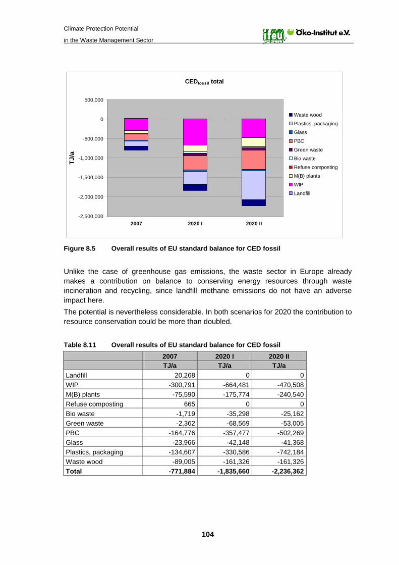
Climate Protection Potential
in the Waste Management Sector
104
CEDfossil total
-2,500,000
-2,000,000
-1,500,000
-1,000,000
-500,000
0
500,000
2007 2020 I 2020 II
TJ/a
Waste wood
Plastics, packaging
Glass
PBC
Green waste
Bio waste
Refuse composting
M(B) plants
WIP
Landfill
Figure 8.5 Overall results of EU standard balance for CED fossil Unlike the case of greenhouse gas emissions, the waste sector in Europe already makes a contribution on balance to conserving energy resources through waste incineration and recycling, since landfill methane emissions do not have an adverse impact here. The potential is nevertheless considerable. In both scenarios for 2020 the contribution to resource conservation could be more than doubled. Table 8.11 Overall results of EU standard balance for CED fossil 2007 2020 I 2020 II TJ/a TJ/a TJ/a Landfill 20,268 0 0 WIP -300,791 -664,481 -470,508 M(B) plants -75,590 -175,774 -240,540 Refuse composting 665 0 0 Bio waste -1,719 -35,298 -25,162 Green waste -2,362 -68,569 -53,005 PBC -164,776 -357,477 -502,269 Glass -23,966 -42,148 -41,368 Plastics, packaging -134,607 -330,586 -742,184 Waste wood -89,005 -161,326 -161,326 Total -771,884 -1,835,660 -2,236,362

Climate Protection Potential
in the Waste Management Sector
105
9 Looking at selected countries
Another part of the study is concerned with looking at three selected countries in an international context. This is intended to show what impact waste management practices with relatively low technology and extensive use of landfill, or even uncontrolled disposal, have in terms of climate effects and resource conservation, compared with Germany and to a large extent the EU 27. The countries selected are Turkey, Tunisia and Mexico. Turkey was selected as a country with strong ambitions to join the EU, while Tunisia and Mexico were chosen as two countries with different degrees of development: whereas Tunisia, incidentally much like Turkey, does not possess any organised nationwide waste management sector, this at least exists in the threshold country Mexico. Another selection criterion was the study and/or data situation. A study on Tunisia (BIFA 2009) was recently performed for the Federal Environment Agency (UBA), and there is also a very comprehensive dissertation on the waste management situation in Tunisia (Cherif 2005). In the case of Mexico, long-standing relations exist with the IFEU through GTZ (development aid) projects. The scenarios examined for the three countries selected are confined to determining the actual situation and a further scenario for 2020. The scenario for 2020 assumes that the waste management sector in the three countries will develop as envisaged for the EU 27 in scenario 2020 I (cf. Chapter 8.2). This assumption is a great simplification and does not take account of possible developments in the countries concerned during the period up to 2020. This would require a more comprehensive study.
9.1 Turkey
According to (EUROSTAT 2009), total municipal waste in Turkey came to around 30 million t. This corresponds to about 430 kg/a per head of the population. An item in (Recycling Magazin 2008) states that about 80% of the waste produced is dumped, often on “wild” rubbish tips. In (bfai 2008) it is claimed that about 100,000 t of the waste is composted. On the basis of this information, it is assumed for the purpose of the balance that a total of 5 million t of the present volume is separately collected and recovered, particularly by the informal sector. With the exception of the composted quantity mentioned, no information is available on the breakdown of the individual recyclable fractions. For the sake of simplicity it is assumed that the breakdown corresponds to the derived EU 27 breakdown for the year 2007. According to the (KfW 2009) there are now 25 controlled landfill sites in Turkey. Roughly half of these sites have gas capture facilities. The captured gas is largely flared off, but on one landfill site the gas is utilised. The mean effective gas capture rate is assumed to be 20%. In addition to the controlled landfill sites there are some 3,000-3,200 “wild” rubbish dumps. Although waste incineration plants exist in Turkey, they only process industrial or special waste (Recycling Magazin 2008). According to (bfai 2008) the quantity of waste deposited on controlled landfill sites in 2006 amounted to 9.95 million t. In terms of the quantity deposited in 2007, this represents about 40%. This means that 60% of waste is dumped on uncontrolled tips.

Climate Protection Potential
in the Waste Management Sector
106
The type of deposition is crucial to their emission potential. If waste is disposed of over a large area, there is scarcely any formation of anaerobic conditions, so little methane is created. If however the waste is deposited in stratified form or in a bed of water, anaerobic conditions are created with associated formation of methane. This means that – purely from a climate protection point of view – uncontrolled disposal of waste over large areas would be preferable to organised deposition. This is a particularly drastic demonstration of how important it is not to lose sight of other environmental impacts in addition to climate protection. Waste disposal practices of this kind give rise to serious environmental problems for the protected assets water, soil and air, and involve great risks for the general public. As regards the waste dumped on uncontrolled tips, the extent to which it is subject to aerobic or anaerobic conditions is not known. Two cases are calculated for the balance: a) half the 60% of waste that is disposed of on uncontrolled tips is spread over large
areas without methane formation, b) all of the 60% of waste that is disposed of on uncontrolled tips is deposited in
stratified form; methane formation is calculated as for controlled landfill sites. The derived waste streams for the two scenarios 2007 Actual and 2020 are shown in Table 9.1. Table 9.1 Waste streams in the two scenarios for Turkey 2007 2020 1,000 t/a % 1,000 t/a % Landfill 25,000 83.3% 0 0% WIP 0 0% 10,858 36.2% M(B) plants 0 0% 3,764 12.5% Refuse composting 0 0% 0 0% Bio waste (bio bin) 0 0% 3,730 12.4% Green waste (total) 100 0.3% 3,702 12.3% PBC 3,023 10.1% 4,070 13.6% Glass 1,033 3.4% 1,391 4.6% Plastics + packaging waste 844 2.8% 1,136 3.8% Waste wood 0 0% 1,349 4.5% Total 30,000 100% 30,000 100%
9.1.1 Greenhouse gas results – Turkey Figure 9.1 and Table 9.5 show the overall balance results for greenhouse gases. Figure 9.2 and Table 9.9 show the overall results of the greenhouse gas balance, with C-sink credits for landfill and pro rata application of green waste compost products to farmland.

Climate Protection Potential
in the Waste Management Sector
107
Greenhouse gases, total
-20,000
-10,000
0
10,000
20,000
30,000
40,000
50,000
2007 2020
1.00
0 t C
O2 e
q/a
Waste wood
Plastics, packaging
Glass
PBC
Green waste
Bio waste
Refuse composting
M(B) plants
WIP
Landfill
Landfill
30% wide-area disposal
0% wide-area disposal
Figure 9.1 Overall results of standard balance for greenhouse gases – Turkey Table 9.2 Overall results of standard balance for greenhouse gases – Turkey 2007 2020 1,000 t CO2 eq/a 1,000 t CO2 eq/a Landfill, 30% wide-area disposal 26,843 0 Landfill, 0% wide-area disposal 39,219 0 WIP 0 -2,573 M(B) plants 0 -852 Refuse composting 0 0 Bio waste 0 -387 Green waste 2 -595 PBC -2,210 -3,596 Glass -480 -647 Plastics + packaging waste -351 -835 Waste wood 0 -1,397 Total (landfill, 0% wide-area) 36,179 -10,882 Total (landfill, 30% wide-area) 23,803 -10,882

Climate Protection Potential
in the Waste Management Sector
108
Greenhouse gases, total with C-sink
-20,000
-10,000
0
10,000
20,000
30,000
40,000
50,000
2007 2020
1.00
0 t C
O2 e
q/a
Waste wood
Plastics, packaging
Glass
PBC
Green waste
Bio waste
Refuse composting
M(B) plants
WIP
Landfill
Landfill
30% wide-areadisposal
0% wide-areadisposal
Figure 9.2 Overall results of greenhouse gas balance with C-sink – Turkey Table 9.3 Overall results of greenhouse gas balance with C-sink – Turkey 2007 2020 1,000 t CO2 eq/a 1,000 t CO2 eq/a Landfill, 30% wide-area disposal 18,597 0 Landfill, 0% wide-area disposal 30,974 0 WIP 0 -2,573 M(B) plants 0 -852 Refuse composting 0 0 Bio waste 0 -435 Green waste 0 -636 PBC -2,210 -3,596 Glass -480 -647 Plastics + packaging waste -351 -835 Waste wood 0 -1,397 Total (landfill, 0% wide-area) 27,932 -10,972 Total (landfill, 30% wide-area) 15,556 -10,972 Regardless of whether a widespread disposal rate of 0% or 30% is assumed for Turkey or whether credits are given for carbon storage (C-sink), deposition of waste as landfill has the most unfavourable effects from a climate protection point of view. Even assuming the most favourable boundary conditions, emissions in Turkey come to more than 15 million t CO2 eq. In the worst case the figure is more than double, at 36 million t CO2 eq. In 2004 Turkey legally became an Annex I member of the United Nations Framework Convention on Climate Change (UNFCCC). Accordingly, two National Inventory Reports have been submitted to the Secretariat of the UNFCCC (NIR Turkey 2007). Tables have also been drawn up in line with the Common Reporting Format (CRF). The latest collection of tables available dated from 2009 for the year 2007. On this basis, Turkey’s

Climate Protection Potential
in the Waste Management Sector
109
national greenhouse gas emissions without land use changes came to 373 million t CO2 eq in 2007. Of this, the “Waste” sector was responsible for about 32 million t CO2 eq or 8.5%. This figure relates exclusively to methane emissions from landfill. This shows that upper end of the range of emissions from landfill is more likely to be correct for the actual situation. Assuming utilisation of the waste quantities hitherto disposed of as landfill, as described above, the waste sector in Turkey can achieve overall savings in the scenario 2020 of between
• 26 million t CO2 eq/a (Table 9.3: taking account of C-sink; difference between total for 2020 and 2007 Actual for 30% wide-area deposition) and
• 47 million t CO2 eq/a (Table 9.2: without C-sink; difference between total for 2020 and 2007 Actual for 0% wide-area deposition).
Whether Turkey has now quantified a reduction target is not clear from (NIR Turkey 2007). However, the greenhouse balance makes it clear that the very extensive measures in the waste management sector for the scenario 2020 could reduce greenhouse gas emissions in Turkey by between 7% (a saving of 26 million t CO2 eq/a, see above) and 13% (a saving of 47 million t CO2 eq/a, see above) compared with 2007. If at least a ban on landfill of organic waste can be successfully introduced, this would reduce greenhouse gases by the 8.5% mentioned above.
9.1.2 Results for fossil energy resources – Turkey Figure 9.3 and Table 9.4 show the overall results of the balance for the conservation of fossil resources, expressed as cumulative fossil energy demand (CED fossil).
CEDfossil total
-250,000
-200,000
-150,000
-100,000
-50,000
0
50,000
2007 2020
TJ/a
Waste wood
Plastics, packaging
Glass
PBC
Green waste
Bio waste
Refuse composting
M(B) plants
WIP
Landfill
Figure 9.3 Overall results of standard balance for CED fossil – Turkey
Unlike the situation for greenhouse gas emissions, the waste sector in Turkey is already making a net contribution to conservation of energy resources. By contrast, landfill has only a slight impact on CED fossil, with a burden resulting from the energy demand. Compared with the actual situation, the scenario 2020 also offers considerable savings potential: the contribution to resource conservation could be more than quadrupled.

Climate Protection Potential
in the Waste Management Sector
110
Table 9.4 Overall results of standard balance for CED fossil – Turkey 2007 2020 TJ/a TJ/a Landfill 4,790 0 WIP 0 -79,991 M(B) plants 0 -21,160 Refuse composting 0 0 Bio waste 0 -4,249 Green waste -14 -8,254 PBC -25,912 -43,033 Glass -3,769 -5,074 Plastics + packaging waste -21,168 -39,796 Waste wood 0 -19,421 Total -46,073 -220,978
9.2 Tunisia
According to (BIFA 2007) the volume of waste in Tunisia in 2007 came to 2.5 million t. In Tunisia, according to (Cherif 2005), waste collection is a local authority duty. There is neither a standardised system nor standardised vehicles. Every municipality seeks to solve the problem individually. The collection vehicles used range from modern collection trucks with built-in compaction equipment to donkey carts or wheelbarrows. In Tunisia’s major cities there is usually a daily waste collection. In the peripheral areas, however, there is a litter problem, especially with plastic packaging. Local authorities generally dump their waste on areas that are no longer in use, e.g. old quarries, dried-out river beds or dried-out salt lakes. As a general rule, uncontrolled disposal results in the waste being spread in thin layers over a certain area (0.5-1.5 m) and not being compacted or covered. In total, there are about 400 uncontrolled tips in Tunisia. These would cost about €90 million to refurbish (Cherif 2005). As of 2005 there were five controlled landfill sites in operation, four of which were almost full. A further nine were under construction. According to (BIFA 2007) there has been little change in this situation. Also according to (BIFA 2007), about half the country’s municipal waste is disposed of on the five controlled landfill sites. The nine landfill sites under construction have been starting to operate successively since 2007. In futures, these will permit controlled deposition of 80% of municipal waste. The existing landfill sites do not have any facilities for landfill gas treatment. Landfill gas is emitted into the atmosphere. In 1997 Tunisia enacted “EcoLef”, a Tunisian packaging ordinance for PET bottles, PE films and tin cans. The relevant licence fees were to be paid by the end of 2003 by fillers/packers and importers on the basis of the packaging-oriented “polluter pays” principle (calculated from the quantity and weight of the packaging material used). At the beginning of 2004 the licence fee was changed to a special levy on imported and locally produced plastic base materials. It is 2.5% of the customs value of plastic base materials for imports, and 2.5% of sales excluding value-added tax for locally produced materials (Cherif 2005).

Climate Protection Potential
in the Waste Management Sector
111
The effective collection rate is still very low, however. According to (BIFA 2007),some 6,000 t of plastic waste was collected in 2007. Packaging waste as a percentage of total municipal waste is around 3.2%, and of this about 4.7% was collected separately (Cherif 2005). These figures can also be found in (BIFA 2007). The same source also states that at present a total about 5% of household waste is sent for recycling. Apart from packaging waste, this largely consists of waste paper and metals. Accordingly, a total recycled quantity of 125,000 t/a is assumed for the scenario 2007, and its assumed breakdown is shown in Table 9.5. Since the breakdown of the scenario 2020 I for the EU 27 does not contain any metals, these are – for the sake of simplicity – kept constant within packaging waste. It is also stated in (BIFA 2007) that about 0.1% of household waste in Tunisia is composted. This small quantity is disregarded here, especially since composting of household waste does not yield any benefits (cf. Chapter 8.3.3). Of the remaining landfill quantity of 2.375 million t/a, the scenario 2007 assumes that half is deposited as controlled landfill, but without gas capture. On the lines of the procedure for Turkey, it was decided that the remaining half of the uncontrolled waste deposits was either
a) all spread over a wide area without any methane formation, or b) all deposited in stratified form with methane formation, as in controlled landfill
sites. The derived waste streams for the two scenarios 2007 and 2020 are shown in Table 9.5. Table 9.5 Waste streams in the two scenarios for Tunisia 2007 2020 1,000 t/a % 1,000 t/a % Landfill 2,375 95.0% 0 0% WIP 0 0% 905 36.2% M(B) plants 0 0% 314 12.5% Refuse composting 0 0% 0 0% Bio waste (bio bin) 0 0% 311 12.4% Green waste (total) 0 0% 309 12.3% PBC 98 3.9% 339 13.6% Glass 0 0% 116 4.6% Plastics + packaging waste 27 1.1% 95 3.8% Waste wood 0 0% 112 4.5% Total 2,500 100% 2,500 100%
9.2.1 Greenhouse gas results – Tunisia Figure 9.4 and Table 9.6 show the overall balance results for greenhouse gases. Figure 9.5 and Table 9.7 show the overall results for greenhouse gases with a C-sink credit for landfill.
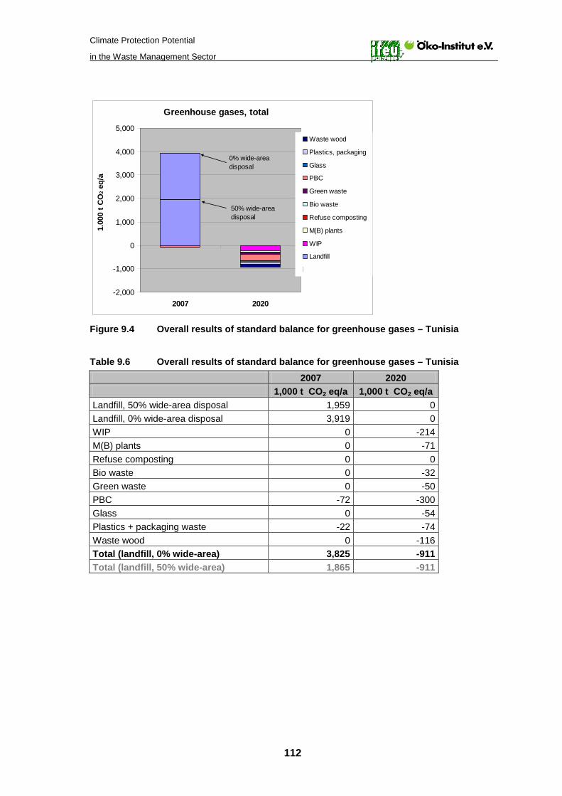
Climate Protection Potential
in the Waste Management Sector
112
Greenhouse gases, total
-2,000
-1,000
0
1,000
2,000
3,000
4,000
5,000
2007 2020
1.00
0 t C
O2 e
q/a
Waste wood
Plastics, packaging
Glass
PBC
Green waste
Bio waste
Refuse composting
M(B) plants
WIP
Landfill
Landfill
50% wide-area disposal
0% wide-areadisposal
Figure 9.4 Overall results of standard balance for greenhouse gases – Tunisia Table 9.6 Overall results of standard balance for greenhouse gases – Tunisia 2007 2020 1,000 t CO2 eq/a 1,000 t CO2 eq/a Landfill, 50% wide-area disposal 1,959 0 Landfill, 0% wide-area disposal 3,919 0 WIP 0 -214 M(B) plants 0 -71 Refuse composting 0 0 Bio waste 0 -32 Green waste 0 -50 PBC -72 -300 Glass 0 -54 Plastics + packaging waste -22 -74 Waste wood 0 -116 Total (landfill, 0% wide-area) 3,825 -911 Total (landfill, 50% wide-area) 1,865 -911
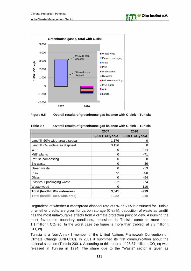
Climate Protection Potential
in the Waste Management Sector
113
Greenhouse gases, total with C-sink
-2,000
-1,000
0
1,000
2,000
3,000
4,000
5,000
2007 2020
1.00
0 t C
O2 e
q/a
Waste wood
Plastics, packaging
Glass
PBC
Green waste
Bio waste
Refuse composting
M(B) plants
WIP
Landfill
Landfill
50% wide-area disposal
0% wide-areadisposal
Figure 9.5 Overall results of greenhouse gas balance with C-sink – Tunisia
Table 9.7 Overall results of greenhouse gas balance with C-sink – Tunisia 2007 2020 1,000 t CO2 eq/a 1,000 t CO2 eq/a Landfill, 50% wide-area disposal 1,176 0 Landfill, 0% wide-area disposal 3,136 0 WIP 0 -214 M(B) plants 0 -71 Refuse composting 0 0 Bio waste 0 -36 Green waste 0 -53 PBC -72 -300 Glass 0 -54 Plastics + packaging waste -22 -74 Waste wood 0 -116 Total (landfill, 0% wide-area) 3,041 -919 Total (landfill, 50% wide-area) 1,082 -919 Regardless of whether a widespread disposal rate of 0% or 50% is assumed for Tunisia or whether credits are given for carbon storage (C-sink), deposition of waste as landfill has the most unfavourable effects from a climate protection point of view. Assuming the most favourable boundary conditions, emissions in Tunisia come to more than 1.1 million t CO2 eq. In the worst case the figure is more than trebled, at 3.8 million t CO2 eq. Tunisia is a Non-Annex I member of the United Nations Framework Convention on Climate Change (UNFCCC). In 2001 it submitted its first communication about the national situation (Tunisia 2001). According to this, a total of 28.87 million t CO2 eq was released in Tunisia in 1994. The share due to the “Waste” sector is given as

Climate Protection Potential
in the Waste Management Sector
114
1.031 million t CO2 eq, which corresponds to about 3.6% of total greenhouse gas emissions. To date there are no more recent communications, and comparison with the emissions determined here is only of limited value because of the different reference years. The figure for the “Waste” is of similar size to the figure calculated here for the best case. If Tunisia were to achieve a ban on landfill and introduce closed substance cycles by 2020, the overall savings would be between:
• 2.0 million t CO2 eq/a (Table 9.7: taking account of C-sink; difference between total for 2020 and 2007 Actual for 50% wide-area deposition) and
• 4,7 million t CO2 eq/a (Table 9.6: without C-sink; difference between total for 2020 and 2007 Actual for 0% wide-area deposition).
It is not known whether Tunisia has quantified a voluntary reduction target. In relation to the total national greenhouse gas emissions in 1994, the possible reduction contributions range from 7% (a saving of 2 million t CO2 eq, see above) to 16% (a saving of 4.7 million t CO2 eq, see above).
9.2.2 Results for fossil energy resources – Tunisia Figure 9.6 and Table 9.8 show the overall results of the balance for the conservation of fossil resources, expressed as cumulative fossil energy demand (CED fossil).
CEDfossil total
-20,000
-15,000
-10,000
-5,000
0
5,000
2007 2020
TJ/a
Waste wood
Plastics, packaging
Glass
PBC
Green waste
Bio waste
Refuse composting
M(B) plants
WIP
Landfill
Figure 9.6 Overall results of standard balance for CED fossil – Tunisia

Climate Protection Potential
in the Waste Management Sector
115
Table 9.8 Overall results of standard balance for CED fossil – Tunisia 2007 2020 TJ/a TJ/a Landfill 455 0 WIP 0 -6,666 M(B) plants 0 -1,763 Refuse composting 0 0 Bio waste 0 -354 Green waste 0 -688 PBC -840 -3,586 Glass 0 -423 Plastics + packaging waste -348 -2,778 Waste wood 0 -1,618 Total -733 -17,877 In the scenario 2007 the low proportionate recycling of suitable materials only makes a small contribution to the conservation of energy resources. By contrast, the scenario 2020 offers considerable savings potential: a 24-fold increase in the contribution to resource conservation would be possible.
9.3 Mexico
Unlike Tunisia and Turkey, Mexico has achieved controlled waste management. Waste is no longer dumped on “wild” tips, but deposited on controlled landfill sites. According to (SEMARNAT, INE 2006a), the volume of waste for 2005 was 0.91 kg/(head*d). This corresponds to about 330 kg/(head*a) or around 35.3 million t/a. In the past, the volume of waste has largely been determined on a sample basis and calculated using the number of inhabitants. For some time now there have been intensive efforts in Mexico to develop waste treatment and management plans including, for example, the establishment of a system for quantitative recording of the entire volume of waste. Mexico has also made a start on the separation collection and recovery of recyclables. According to (SEMARNAT, INE 2006a) about 7% of total waste was recycled in 2004. The largest component of total waste is the organic fraction, at 53%. Three percent of the organic waste was separately collected and recovered; here it is counted as green waste. The remaining recyclable fractions collected separately are paper (14% in residual waste, 16% separately collected), glass (13% of 6% in residual waste), plastics (8% of 4% in residual waste) and metals (80% of 3% in residual waste). The resulting waste streams for 2005 are shown in Table 9.9. Here too, as in the case of Tunisia, the quantity of metal within packaging waste is kept constant in the scenario 2020 for simplicity’s sake, since the underlying scenario 2020 I for the EU 27 does not include a metal fraction. The remaining 19% of miscellaneous waste in residual waste consists largely of wood, leather, rubber and textiles. These are materials which could potentially be recycled, but at great expense. It is estimated in (SEMARNAT, INE 2006a) that, all in all, around 28% of the total volume of waste would potentially be available for recycling, which amounts to about 10 million t/a.

Climate Protection Potential
in the Waste Management Sector
116
Table 9.9 Waste streams in the two scenarios for Mexico 2005 2020 1,000 t/a % 1,000 t/a % Landfill 32,766 92.7% 0 0% WIP 0 0% 12,797 36.2% M(B) plants 0 0% 4,436 12.5% Refuse composting 0 0% 0 0% Bio waste (bio bin) 0 0% 4,396 12.4% Green waste (total) 562 1.6% 4,364 12.3% PBC 792 2.2% 4,797 13.6% Glass 276 0.8% 1,639 4.6% Plastics + packaging waste 962 2.7% 1,339 3.8% Waste wood 0 0% 1,590 4.5% Total 35,358 100.0% 35,358 100.0% As of 2005, the quantity deposited as landfill comes to about 32.8 million t/a. About 20% is deposited on controlled landfill sites with gas capture, and about 80% on controlled landfill sites without gas capture. As in the standard for the EU 27, the effective gas capture rate is assumed to be 20%. In Mexico, about 80% of the captured landfill gas is utilised in CHP plants, and about 20% of the captured landfill gas is flared off (Aguilar 2009). A sensitivity analysis for Mexico considers the case that all landfill sites have gas capture facilities.
9.3.1 Greenhouse gas results – Mexico Figure 9.7 and Table 9.10 show the overall balance results for greenhouse gases. Figure 9.8 and Table 9.11 show the overall results of the greenhouse gas balance, with C-sink credits for landfill and pro rata application of green waste compost products to farmland.
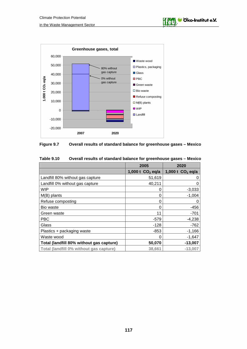
Climate Protection Potential
in the Waste Management Sector
117
Greenhouse gases, total
-20,000
-10,000
0
10,000
20,000
30,000
40,000
50,000
60,000
2007 2020
1.00
0 t C
O2 e
q/a
Waste wood
Plastics, packaging
Glass
PBC
Green waste
Bio waste
Refuse composting
M(B) plants
WIP
Landfill
Landfill
0% without gas capture
80% withoutgas capture
Figure 9.7 Overall results of standard balance for greenhouse gases – Mexico Table 9.10 Overall results of standard balance for greenhouse gases – Mexico 2005 2020 1,000 t CO2 eq/a 1,000 t CO2 eq/a Landfill 80% without gas capture 51,619 0 Landfill 0% without gas capture 40,211 0 WIP 0 -3,033 M(B) plants 0 -1,004 Refuse composting 0 0 Bio waste 0 -456 Green waste 11 -701 PBC -579 -4,238 Glass -128 -762 Plastics + packaging waste -853 -1,166 Waste wood 0 -1,647 Total (landfill 80% without gas capture) 50,070 -13,007 Total (landfill 0% without gas capture) 38,661 -13,007

Climate Protection Potential
in the Waste Management Sector
118
Greenhouse gases, total with C-sink
-20,000
-10,000
0
10,000
20,000
30,000
40,000
50,000
60,000
2007 2020
1.00
0 t C
O2
eq/a
Waste wood
Plastics, packaging
Glass
PBC
Green waste
Bio waste
Refuse composting
M(B) plants
WIP
Landfill
Landfill
0% withoutgas capture
80% withoutgas capture
Figure 9.8 Overall results of greenhouse gas balance with C-sink – Mexico Table 9.11 Overall results of greenhouse gas balance with C-sink – Mexico 2005 2020 1,000 t CO2 eq/a 1,000 t CO2 eq/a Landfill 80% without gas capture 40,733 0 Landfill 0% without gas capture 29,324 0 WIP 0 -3,033 M(B) plants 0 -1,004 Refuse composting 0 0 Bio waste 0 -513 Green waste 1 -750 PBC -579 -4,238 Glass -128 -762 Plastics + packaging waste -853 -1,166 Waste wood 0 -1,647 Total (landfill 80% without gas capture) 39,174 -13,114 Total (landfill 0% without gas capture) 27,765 -13,114 Regardless of whether the gas capture rate on landfill sites in Mexico is assumed to be 20%, as at present, or 100%, or whether credits are given for carbon storage (C-sink), deposition of waste as landfill has the most unfavourable effects from a climate protection point of view. Assuming the most favourable boundary conditions with complete gas capture and C-sink credits, nearly 28 million t CO2 eq is emitted in Mexico every year. Without C-sink credits and with the present gas capture of only 20%, the annual greenhouse gas emissions are nearly twice as high, at 50 million t CO2 eq. Mexico is a Non-Annex I member of the UNFCCC and has already submitted its third communication about the national situation (SEMARNAT, INE 2006b). According to this, a total of around 643 million t of greenhouse gas emissions were released in Mexico in

Climate Protection Potential
in the Waste Management Sector
119
2002. The share of the “waste” sector is given as 10% of total emissions or about 65.6 million t CO2 eq. After allowing for the different reference years, this figure corresponds roughly to the figure calculated here without C-sink credit. The Kyoto Protocol does not recognise the C-sink for the purpose of national reporting (IPCC 2006). If Mexico were to achieve a ban on landfill and the establish further closed substance cycles by 2020, the overall savings would be between:
• 41 million t CO2 eq/a (Table 9.11: taking account of C-sink; difference between total for 2020 and 2007 Actual for 0% without gas capture) and
• 63 million t CO2 eq/a (Table 9.10: without C-sink; difference between total for 2020 and 2007 Actual for 80% without gas capture).
It is not known whether Mexico has quantified a voluntary reduction target. In relation to the total national greenhouse gas emissions in 2002, the possible reduction contributions range from about 6% (a saving of 41 million t CO2 eq, see above) to 10% (a saving of 63 million t CO2 eq, see above).
9.3.2 Results for fossil energy resources – Mexico Figure 9.9 and Table 9.12 show the overall results of the balance for the conservation of fossil resources, expressed as cumulative fossil energy demand (CED fossil).
CEDfossil total
-300,000
-250,000
-200,000
-150,000
-100,000
-50,000
0
50,000
2007 2020
TJ/a
Waste woodPlastics, packagingGlassPBCGreen wasteBio wasteRefuse compostingM(B) plantsWIPLandfill
Figure 9.9 Overall results of standard balance for CED fossil – Mexico
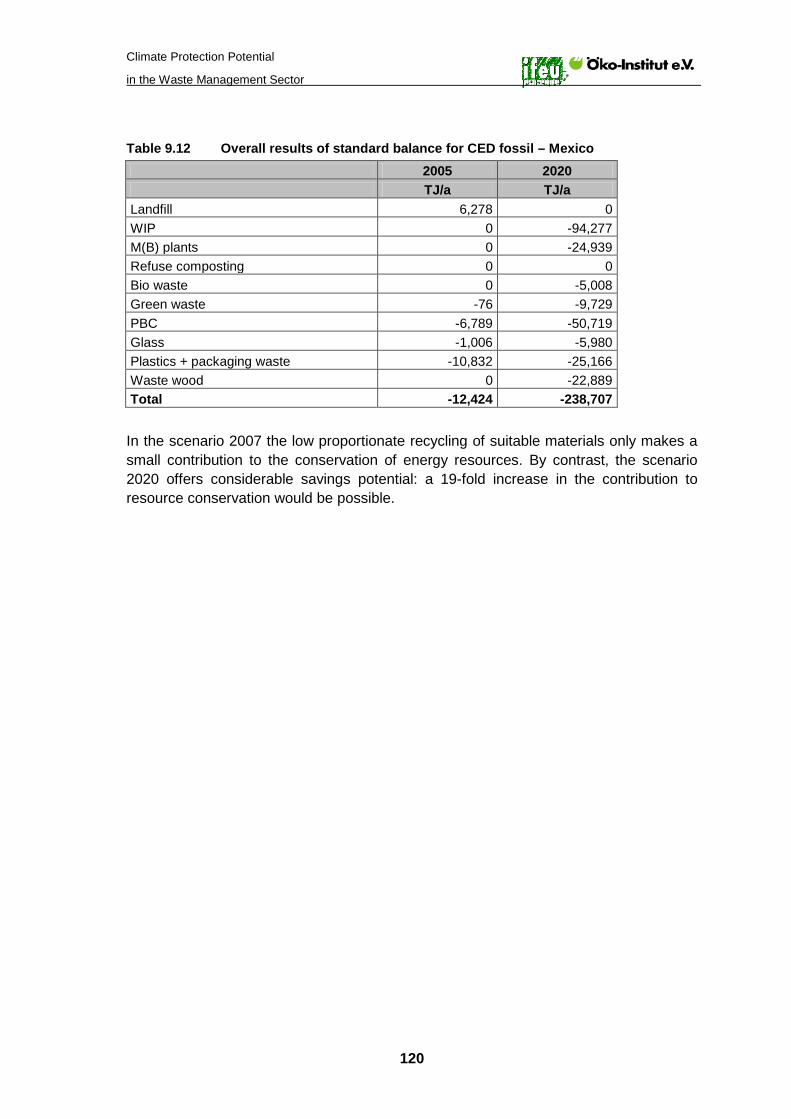
Climate Protection Potential
in the Waste Management Sector
120
Table 9.12 Overall results of standard balance for CED fossil – Mexico 2005 2020 TJ/a TJ/a Landfill 6,278 0 WIP 0 -94,277 M(B) plants 0 -24,939 Refuse composting 0 0 Bio waste 0 -5,008 Green waste -76 -9,729 PBC -6,789 -50,719 Glass -1,006 -5,980 Plastics + packaging waste -10,832 -25,166 Waste wood 0 -22,889 Total -12,424 -238,707 In the scenario 2007 the low proportionate recycling of suitable materials only makes a small contribution to the conservation of energy resources. By contrast, the scenario 2020 offers considerable savings potential: a 19-fold increase in the contribution to resource conservation would be possible.

Climate Protection Potential
in the Waste Management Sector
121
10 Summary
10.1 Goals and method
By ratifying the Kyoto Protocol, Germany undertook to make annual reports to the United Nations Framework Convention on Climate Change (UNFCCC) about Germany’s emissions of greenhouse gases. This is done in the National Inventory Report (NIR), which under the Common Reporting Format (CRF) is required to observe a specific organisation. This means that waste management aspects are only to be found in the “Waste” sector. However, this sector includes only those greenhouse gas emissions which are associated with landfill, biological treatment (including biological treatment in M(B) plants), and incineration without energy generation. By contrast, the benefits of waste recovery as material or energy are integrated in other sectors (“Energy”, “Industrial Process”). This method of reporting is practical for the purposes of the National Inventory Reports, i.e. compliance with the national reduction targets. It is not, however, suitable for presenting the successes achieved by the waste management sector as a service industry, since it does not clearly show the benefits of waste management that accrue in other sectors. This study uses the life cycle assessment method to determine the climate protection potential of the waste management sector, examining the example of municipal waste and waste wood. Life cycle assessment investigates all process steps such as collection, treatment and recovery of secondary products from the moment the waste is produced, and also includes the relevant benefits generated, such as substitution of primary raw materials and energy. This study assesses the contributions currently made by municipal waste management in Germany, the EU 27 and, in a first inventory, the countries Turkey, Tunisia and Mexico through separate collection of recyclable fractions from municipal waste and their recovery as material and energy. In addition it examines the waste wood fraction in view of its special importance for climate protection. In the case of Germany this is not confined to the municipal waste management sector, but is also extended to include waste wood from all sources. The possible optimisation measures from a climate protection point of view are determined in scenarios for the year 2020. For the waste management sector in Germany, the optimisation potential is assessed separately in terms of technical measures (scenario 2020 T) and waste stream steering measures (scenario 2020 A), and as a combination of these two scenarios (2020 AT). In the EU 27, and especially in the three countries selected as example, landfill still plays a significant or even dominant role. For these countries the main focus of the optimisation scenarios for 2020 is on the complete discontinuation of landfill. This measure, which by avoiding methane emissions makes a significant contribution to climate protection, has already been completely implemented in Germany (Öko-Institut/IFEU 2005). The scenario with technical measures for Germany assumes in particular efficiency improvements in plants for energy utilisation and to some extent in recycling as material (cf. Chapters 4.3 to 4.10). The quantities of the waste streams are kept constant. The measures to influence waste streams are concerned with increasing separate collection

Climate Protection Potential
in the Waste Management Sector
122
of recyclables from household waste and redirecting individual waste streams within the treatment paths (cf. Chapter 4.1). One objective of the study is to ascertain the system performance of the municipal waste sector by totalling the individual fractions. In doing so it is possible to analyse not only the contributions of the individual waste fractions such as waste paper recycling or residual waste disposal, but also the overall performance of the waste sector, but not specific treatment technologies. The achievements of the individual treatment technologies such as waste incineration plants are therefore found not only under direct combustion but also under the various treatment paths such as M(B) plants, LWP, bio waste etc. In view of the question, the assessment is restricted to the criteria climate protection and conservation of energy resources. As a result, it ignores important contributions by the waste management sector such as savings in mineral resources or the environmental impacts of acidification and eutrophication. The removal of pollutants from the animate environment by waste incineration is not taken into account either (cf. Öko-Institut 2008d). For a final, comprehensive assessment of appropriate measures for developing and improving the municipal waste management sector it would be necessary to undertake a full life cycle assessment taking account of all environmental achievements. Furthermore, the scenarios for 2020 are not – and cannot be – specific action recommendations for the further development of the municipal waste management sector. For this purpose it would be necessary to extend the assessment to include additional environmental impacts, and in particular to undertake detailed studies of technical feasibility, implementation possibilities such as site conditions, and the cost of the measures. Such aspects do not form part of this study, however. Instead it explores and identifies the potential of the municipal waste sector to take advantage of optimisation measures and aim for the upper limits of what is feasible. Whether, in the final analysis, these measures are suitable for and capable of concrete implementation, and how cost-effective they are, are questions that basically have to be investigated in the individual case. To test the robustness of the findings, having regard to data uncertainties, sensitivity analyses are performed for the greenhouse gas balance in Germany.
10.2 Results
When evaluating the results, it must be borne in mind that within the waste management sector the assessment covered only the two fields:
• municipal waste and • waste wood recycling (in Germany this includes wood from construction and
demolition waste, packaging etc.). The waste management sector as a whole would probably display considerably great potential, as indicated by the relative waste quantities for Germany in 2006:
• Total volume of waste: 372.9 million t • Municipal waste considered 42.7 million t (11.4% of total quantity) • Waste wood volume 6.9 million t (1.9% of total quantity)
These proportions are more or less correct for the EU 27 as well.

Climate Protection Potential
in the Waste Management Sector
123
10.2.1 Results of balance for Germany The main results of the study for Germany are set out briefly below.
Greenhouse gases Today the municipal waste sector, together with waste wood utilisation, is already contributing a saving of about 18 million t CO2 eq to climate protection. In 1990 the municipal waste sector was still a polluter responsible for some 38 million t CO2 eq of Germany’s total emissions. Thus the overall reduction since 1990 amounts to 56 million t CO2 eq/a35
Including waste wood utilisation, and assuming that all optimisation measures in the assessment for 2020 are implemented, the municipal waste sector’s contribution to reducing greenhouse gas emissions increases to about 65 million t CO2 eq/a
or about 670 kg CO2 eq/(head*a). This corresponds to about 24% of the total decrease of 235 million t CO2 eq/a or 2.8 t CO2 eq/(head*a) achieved from 1990 to 2006, according to the National Inventory Report.
36
All waste fractions contribute to the successes of the municipal waste sector on the climate protection front: not only the utilisation of residual waste in waste incineration plants and M(B) plants, but also the separate collection and recovery of recyclables. The utilisation of the entire waste wood occurring in Germany also makes a substantial contribution (see
or 790 kg CO2 eq/(head*a). By 2020 Germany is aiming to reduce greenhouse gas emissions by 40% compared with 1990. This corresponds to a total of 486 million t CO2 eq/a or 5.9 t CO2 eq/(head*a). On the basis of the figures mentioned above, the municipal waste sector’s potential contribution to this targeted reduction is around 13%.
Table 10.1). Table 10.1 Overall results of standard balance for greenhouse gases in Germany, with
a breakdown of the individual contributions of residual waste, separately collected recyclables and waste wood
2006 Actual 2020 T 2020 A 2020 AT 1,000 t
CO2 eq/a 1,000 t
CO2 eq/a 1,000 t
CO2 eq/a 1,000 t
CO2 eq/a Residual waste disposal -2,344 -6,009 -1,435 -3,861 Recovery of separately collected recyclables -8,926 -11,589 -11,356 -15,308 Waste wood recycling -6,503 -7,897 -6,834 -8,299 Total -17,773 -25,496 -19,625 -27,468
It is interesting to compare the greenhouse gas reduction of approx. 18 million t CO2 eq already achieved by the municipal waste sector and waste wood utilisation in 2006 with the greenhouse gas emissions produced by car traffic: at present an average car emits about 180 g CO2/km. Assuming that the average annual mileage per car is around 13,000 km, the achievements of the municipal waste sector in Germany cancel out the
35 It must be remembered that the balance for 1990 did not include waste wood. Without waste wood the saving is in the region of 49 million t CO2 eq/a (cf. also Chapter 7). 36 Without waste wood the saving is in the region of 57 million t CO2 eq/a (cf. Footnote 35).

Climate Protection Potential
in the Waste Management Sector
124
CO2 emissions of 7.7 million cars. This corresponds to nearly 19% of the 41.3 million cars on the road in Germany (www.kba.de). The sensitivity analyses show that the results of the standard balance can be described as robust. Even if the fluctuations are considerable after allowing for all individual analyses, the overall trend of the results remains stable.
Fossil energy resources Today the German municipal waste sector, together with waste wood utilisation, is already contributing approx. 325 PJ/a to savings in fossil energy resources, expressed as CEDfossil. By 2020 this contribution could increase to 455 PJ, assuming that scenario 2020 AT is implemented. In 2006 the total consumption of fossil primary energy in Germany came to about 12,000 PJ (DIW 2007). Given 82.4 million people in Germany, this represents an average consumption of 146 GJ per person per year. On this basis, the contribution of the municipal waste sector and waste wood recovery in 2006 corresponds to the average consumption of about 2 million persons. If one translates the savings from the scenario 2020 AT into present-day average consumption per head of the population, they make it possible to meet the requirements of 3 million people. Table 10.2 shows the contributions to the conservation of fossil energy resources that are made by the utilisation of residual waste in waste incineration plants and M(B) plants, the separate collection and recovery of recyclables, and waste wood recycling. Table 10.2 Overall results of standard balance for conservation of fossil energy
resources in Germany, with a breakdown of the individual contributions of residual waste, separately collected recyclables and waste wood
2006 Actual 2020 T 2020 A 2020 AT TJ/a TJ/a TJ/a TJ/a
Residual waste disposal -96,176 -139,076 -63,881 -93,110 Recovery of separately collected recyclables -149,393 -193,640 -195,391 -254,332 Waste wood recycling -79,140 -102,433 -83,164 -107,641 Total -324,708 -435,148 -342,436 -455,083
Discrepancies in the totals are due to rounding differences
10.2.2 Results of the balance for the EU 27 The main results of the study for the EU 27 are set out below.
Greenhouse gases The results of the assessment for the municipal waste sector in the EU 27, including waste wood recycling, are not based on data of comparable quality and depth to the data used for the assessments in Germany. The results can nevertheless be regarded as a good guide to the potential that exists in the EU 27. In 2007 the contribution to greenhouse gas emission reductions that is made by the municipal waste sector in the EU 27, including waste wood recycling, was still strongly influenced by the fact that some 106 million t of municipal waste was deposited as
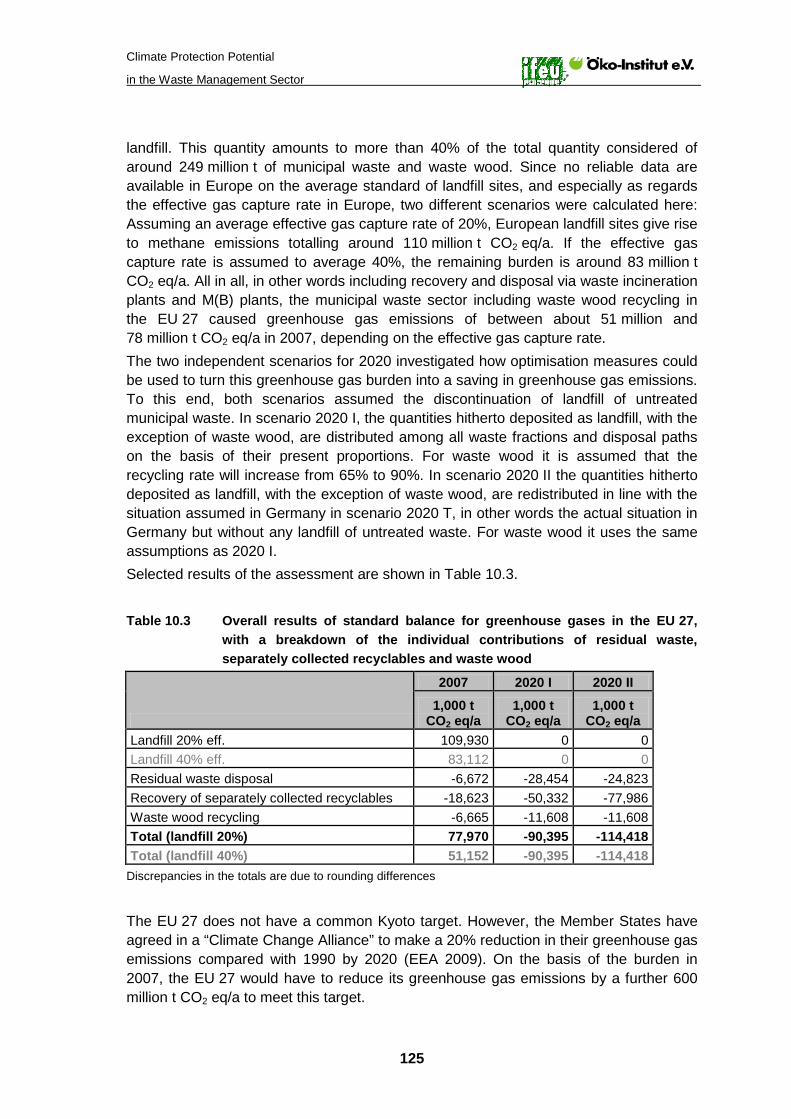
Climate Protection Potential
in the Waste Management Sector
125
landfill. This quantity amounts to more than 40% of the total quantity considered of around 249 million t of municipal waste and waste wood. Since no reliable data are available in Europe on the average standard of landfill sites, and especially as regards the effective gas capture rate in Europe, two different scenarios were calculated here: Assuming an average effective gas capture rate of 20%, European landfill sites give rise to methane emissions totalling around 110 million t CO2 eq/a. If the effective gas capture rate is assumed to average 40%, the remaining burden is around 83 million t CO2 eq/a. All in all, in other words including recovery and disposal via waste incineration plants and M(B) plants, the municipal waste sector including waste wood recycling in the EU 27 caused greenhouse gas emissions of between about 51 million and 78 million t CO2 eq/a in 2007, depending on the effective gas capture rate. The two independent scenarios for 2020 investigated how optimisation measures could be used to turn this greenhouse gas burden into a saving in greenhouse gas emissions. To this end, both scenarios assumed the discontinuation of landfill of untreated municipal waste. In scenario 2020 I, the quantities hitherto deposited as landfill, with the exception of waste wood, are distributed among all waste fractions and disposal paths on the basis of their present proportions. For waste wood it is assumed that the recycling rate will increase from 65% to 90%. In scenario 2020 II the quantities hitherto deposited as landfill, with the exception of waste wood, are redistributed in line with the situation assumed in Germany in scenario 2020 T, in other words the actual situation in Germany but without any landfill of untreated waste. For waste wood it uses the same assumptions as 2020 I. Selected results of the assessment are shown in Table 10.3. Table 10.3 Overall results of standard balance for greenhouse gases in the EU 27,
with a breakdown of the individual contributions of residual waste, separately collected recyclables and waste wood
2007 2020 I 2020 II 1,000 t
CO2 eq/a 1,000 t
CO2 eq/a 1,000 t
CO2 eq/a Landfill 20% eff. 109,930 0 0 Landfill 40% eff. 83,112 0 0 Residual waste disposal -6,672 -28,454 -24,823 Recovery of separately collected recyclables -18,623 -50,332 -77,986 Waste wood recycling -6,665 -11,608 -11,608 Total (landfill 20%) 77,970 -90,395 -114,418 Total (landfill 40%) 51,152 -90,395 -114,418
Discrepancies in the totals are due to rounding differences
The EU 27 does not have a common Kyoto target. However, the Member States have agreed in a “Climate Change Alliance” to make a 20% reduction in their greenhouse gas emissions compared with 1990 by 2020 (EEA 2009). On the basis of the burden in 2007, the EU 27 would have to reduce its greenhouse gas emissions by a further 600 million t CO2 eq/a to meet this target.

Climate Protection Potential
in the Waste Management Sector
126
The possible EU 27 reduction potentials for 2020 compared with 2007 range from 142 to 192 million t CO2 eq/a depending on the scenario and the effective gas capture rate assumed. This corresponds to 24% or 32% of the additional reduction of 600 million t CO2 eq needed to achieve the joint reduction target for 2020. From a climate protection point of view, a strict ban on landfill of untreated waste following the example set by Germany, Austria or Switzerland would make the crucial contributions to improving the climate protection balance of the waste management sector. It is also an essential precondition for significant optimisation in the EU 27.
Fossil energy resources In 2007 the European municipal waste sector, together with waste wood recycling, was already contributing approx. 772 PJ/a to savings in fossil energy resources, expressed as CEDfossil. Unlike the climate balance, landfill methane emissions do not make themselves felt in the assessment for fossil energy resources. By 2020 this contribution could increase to 2,236 PJ/a, assuming that scenario 2020 II is implemented. Table 10.4 Overall results of standard balance for conservation of fossil energy
resources in the EU 27, with a breakdown of the individual contributions of residual waste, separately collected recyclables and waste wood
2007 2020 I 2020 II TJ/a TJ/a TJ/a
Landfill 20,268 0 0 Residual waste recycling -375,716 -840,255 -711,048 Recovery of separately collected recyclables -327,430 -834,078 -1,363,987 Waste wood recycling -89,005 -161,326 -161,326 Total -771,883 -1,835,659 -2,236,361
10.2.3 Results of the assessments for Turkey, Tunisia and Mexico Only very limited data are available for the selected countries Turkey, Tunisia and Mexico. Landfill is the dominant solution in these countries. In Turkey and Tunisia, uncontrolled landfill of waste is usual. Mexico, by contrast, has at least succeeded in establishing a controlled waste management sector. The results of the greenhouse gas assessment 2007 for all three countries are therefore dominated by methane emissions from controlled and uncontrolled landfill. In uncontrolled landfill it is important to distinguish between waste thrown away over a wide area and waste deposited in stratified form. In view of the aerobic conditions, wide-area disposal produces very little methane. This is a particularly drastic example of how important it is not to lose sight of other environmental impacts in addition to climate protection. Uncontrolled deposition of waste gives rise to serious environmental problems for the protected assets water, soil and air, and involves great risks to the general public.
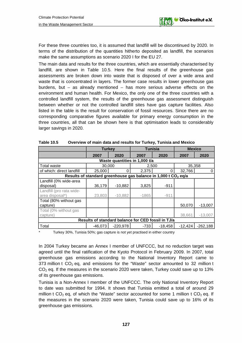
Climate Protection Potential
in the Waste Management Sector
127
For these three countries too, it is assumed that landfill will be discontinued by 2020. In terms of the distribution of the quantities hitherto deposited as landfill, the scenarios make the same assumptions as scenario 2020 I for the EU 27. The main data and results for the three countries, which are essentially characterised by landfill, are shown in Table 10.5. Here the final results of the greenhouse gas assessments are broken down into waste that is disposed of over a wide area and waste that is concentrated in layers. The former case results in lower greenhouse gas burdens, but – as already mentioned – has more serious adverse effects on the environment and human health. For Mexico, the only one of the three countries with a controlled landfill system, the results of the greenhouse gas assessment distinguish between whether or not the controlled landfill sites have gas capture facilities. Also listed in the table is the result for conservation of fossil resources. Since there are no corresponding comparative figures available for primary energy consumption in the three countries, all that can be shown here is that optimisation leads to considerably larger savings in 2020. Table 10.5 Overview of main data and results for Turkey, Tunisia and Mexico Turkey Tunisia Mexico 2007 2020 2007 2020 2007 2020
Waste quantities in 1,000 t/a Total waste 30,000 2,500 35,358 of which: direct landfill 25,000 0 2,375 0 32,766 0
Results of standard greenhouse gas balance in 1,000 t CO2 eq/a Landfill (0% wide-area disposal) 36,179 -10,882 3,825 -911 Landfill (pro rata wide-area disposal*) 23,803 -10,882 -1865 -911 Total (80% without gas capture) 50,070 -13,007 Total (0% without gas capture) 38,661 -13,007
Results of standard balance for CED fossil in TJ/a Total -46,073 -220,978 -733 -18,458 -12,424 -262,188
* Turkey 30%, Tunisia 50%; gas capture is not yet practised in either country
In 2004 Turkey became an Annex I member of UNFCCC, but no reduction target was agreed until the final ratification of the Kyoto Protocol in February 2009. In 2007, total greenhouse gas emissions according to the National Inventory Report came to 373 million t CO2 eq, and emissions for the “Waste” sector amounted to 32 million t CO2 eq. If the measures in the scenario 2020 were taken, Turkey could save up to 13% of its greenhouse gas emissions. Tunisia is a Non-Annex I member of the UNFCCC. The only National Inventory Report to date was submitted for 1994. It shows that Tunisia emitted a total of around 29 million t CO2 eq, of which the “Waste” sector accounted for some 1 million t CO2 eq. If the measures in the scenario 2020 were taken, Tunisia could save up to 16% of its greenhouse gas emissions.
Climate Protection Potential
in the Waste Management Sector
128
Mexico, also a Non-Annex I member of the UNFCCC, has already submitted its third National Inventory Report. The latest report for the year 2002 shows that Mexico emitted a total of around 643 million t CO2 eq, of which the “Waste” sector accounted for some 65.6 million t CO2 eq. If Mexico implemented the measures in the scenario 2020, the country could reduce its total greenhouse gas emissions by up to 10%.
10.3 Conclusion
A direct comparison of the results for Germany, the EU 27 and the three selected countries is not possible, since the framework conditions differ from case to case and the comparisons are based on different reference quantities depending on the information available. In qualitative terms, however, it is possible to state as a general conclusion that phasing out landfill makes a decisive contribution to climate protection. This has already been done in Germany. Here the reduction due to the municipal waste sector is currently around 24% of the greenhouse gas reduction according to the National Inventory Report. In the years between now and 2020 the municipal waste sector can make a further contribution to greenhouse gas reduction, though not such a dramatic one as was achieved by the end of landfill. The municipal waste sector in Germany can contribute up to 13% of the target of a 40% reduction by 2020 compared with 1990. The EU 27 still releases up to 110 million t CO2 eq from landfill every year. Simply phasing out landfill would make a major additional contribution to climate protection. For the EU 27, unlike Germany, no base year in the past was investigated for comparison purposes, so it is not possible to make statements about any greenhouse gas reduction contributions which the EU 27 may already have made to climate protection. However, on the basis of the assessment year 2007, the municipal waste sector in the EU 27 could contribute up to 32% to the EU 27 reduction target for 2020. Landfill is also the dominant source of greenhouse gas emissions in the waste sector in Turkey, Tunisia and Mexico. These countries have yet to agree reduction targets. However, if the potential reduction results – primarily of phasing out landfill – are seen in relation to the present greenhouse gas emissions of the three countries, the municipal waste sector can contribute up to 13% in Turkey, up to 16% in Tunisia and up to 10% in Mexico.
Climate Protection Potential
in the Waste Management Sector
129
11 Bibliography
AEA 2001 AEA Technology Environment: Waste Management Options and Climate Change. Final Report to the European Commission, DG Environment. July, 2001
Aguilar 2009 Persönliche Mitteilung M. en I. Guillermo Encarnación Aguilar, Subdirector de Investigación sobre el Manejo Integral los Residuos, Centro Nacional de Investigación y Capacitación Nacional del Instituto Nacional de Ecología México, 2009
AWM 2007 Abfallwirtschaftsbetriebe Münster: Abfallwirtschaftskonzept der Stadt Münster 2007, Münster, November 2007
Barth 2009 Barth, M., BSR Berlin, e-mail dated 8.07.2009 BAV 2009a Bundesverband der Altholzaufbereiter und -verwerter e.V.:
Personal communication from Ms Boelling to BDE dated 29.5.2009
BAV 2009b Stellungnahme des Bundesverbandes der Altholzaufbereiter und -verwerter e.V. zur Studie vom 10.7.2009
BayLfU 2003 Zusammensetzung und Schadstoffgehalt von Siedlungs-abfällen. Bayerisches Landesamt für Umweltschutz (Ed.), Augsburg, 2003
bfai 2008 Türkei entdeckt das Abfallrecycling. Datenbank Länder und Märkte der Bundesagentur für Außenwirtschaft (bfai), 4.07.2008
BGK 2004 Excerpts from a presentation by Mr Kehres dated 2004, supplied by UBA
BGK 2008 Kompostanwendung 2007. Written communication BGK, Dec. 2008
BGK 2009 Zusammensetzung von Bioabfällen in Vergärungsanlagen. Auswertung der BGK in: H&K aktuell 7/8 2009, p. 8
BIFA 2009 Text excerpts kindly supplied from a UBA study on Tunisia BMU 2008 Bundesministerium für Umwelt, Naturschutz und Reaktor-
sicherheit: „Erneuerbare Energien in Zahlen – Nationale und internationale Entwicklung“, Berlin/Bonn, June 2008
Cherif 2005 Cherif, M.: Strukturen und Entwicklungspotenziale der Abfallwirtschaft in Tunesien. Dissertation an der RWTH Aachen, Fakultät für Bauingenieurwesen, August 2005
Dehoust/Giegrich 2003 Dehoust, G., Giegrich, J.: Critical Review: „Beurteilung der Umweltverträglichkeit von thermischen Entsorgungs-maßnahmen; Leitfaden Sekundärbrennstoffe“, im Auftrag des Ministeriums für Umwelt und Naturschutz, Landwirtschaft und Verbraucherschutz des Landes Nord-rhein-Westfalen, Öko-Institut e. V., Institut für Energie- und

Climate Protection Potential
in the Waste Management Sector
130
Umweltforschung Heidelberg (IFEU) GmbH; Darmstadt/-Heidelberg, 2003
DBU 2002 Vogt, R., Knappe, F., Giegrich, J., Detzel, A., IFEU Heidel-berg: Ökobilanz Bioabfallverwertung. Gefördert von der Deutschen Bundesstiftung Umwelt (DBU). Initiativen zum Umweltschutz 52. Erich Schmidt Verlag, Berlin 2002
DIW 2007 DIW Berlin: Wochenbericht No. 8/2007 EC 2009 Study on the selection of waste streams for End of Waste
assessment. European Commission, Joint Research Centre (JRC), Institute for Prospective Technological Studies (ipts), 2009
Ecoinvent 2007 Ecoinvent Data v.2.0. Ecoinvent report No. 13_I (Waste treatment_General)
EdDE 2005 Bilitewski, B. et al.: Ökologische Effekte der Müllverbren-nung durch Energienutzung“. Entsorgergemeinschaft der Deutschen Entsorgungswirtschaft e.V., Pirna, December 2005
EdDE 2007 Gottschall, R. (Humus & Erden Kontor GmbH), Kranert, M. (ISWA), et al.: Grünabfälle – besser kompostieren oder energetisch verwerten? – Vergleich unter den Aspekten der CO2-Bilanz und der Torfsubstitution – Entsorgergemein-schaft der Deutschen Entsorgungswirtschaft e.V. (EdDE), Cologne, December 2007
EdDE 2009 Widmann, R. et al.: Bewertung der Kohlenstoffeinbindung in Böden durch Kompost. Literaturstudie im Auftrag der Entsorgergemeinschaft der Deutschen Entsorgungswirt-schaft (EdDE) e.V., January 2009
EEA 2009 European Environment Agency: Annual European Community greenhouse gas inventory 1990 – 2007 an inventory report 2009 – Submission to the UNFCC Secretariat, Copenhagen 2009
EEG Monitoring 2008 Anschlussvorhaben zum Monitoring zur Wirkung des novellierten Erneuerbare-Energien-Gesetzes (EEG) auf die Entwicklung der Stromerzeugung aus Biomasse. IE Leipzig, Fichtner Stuttgart, TLL Jena, Prof. Dr. jur. Stefan Klinski Berlin. Im Auftrag des Bundesministerium für Umwelt, Naturschutz und Reaktorsicherheit (BMU), March 2008
ETC RWM 2008 Skovgaard, M., Hedal, N., Villanueva, A. (European Topic Centre on Resource and Waste Management) and Moller Andersen, F., Larsen, H. (Technical University of Denmark): Municipal Waste Management and Greenhouse Gases. ETC/RWM working paper 2008/1
ETC 2009 EU Achievements, Opportunities and Barriers to reduce waste management GHG emissions. European Topic Centre on Sustainable Consumption and Production (ETC)

Climate Protection Potential
in the Waste Management Sector
131
under contract with the European Environment Agency, presentation Christian Fischer 2009
FZKA 2003 Leible, L., Arlt, A., Fürniß, B., Kälber, S., Kappler, G., Lange, S., Nieke, E., Rösch, C., Wintzer, D.: Energie aus biogenen Rest- und Abfallstoffen. Forschungszentrum Karlsruhe, Institut für Technikfolgenabschätzung und Systemanalyse. Wissenschaftliche Berichte FZKA 6882. July 2003
Gebhardt 2005 Gebhardt, P.: „Quecksilberemissionen durch die Müll-verbrennung“, Salzböden 2005
GEMIS 1994 „Umweltanalyse von Energie-, Transport- und Stoff-systemen – Gesamt-Emissions-Modell Integrierter Systeme (GEMIS) – Version 2.1, aktualisierter und erweiterter Endbericht“; Öko-Institut e. V., i. A. des Hessischen Ministeriums für Umwelt, Energie, und Bundesangelegen-heiten, Darmstadt/Kassel 1994
GEMIS 2008 „Globales Emissions-Modell Integrierter Systeme (GEMIS), Version 4.4“; Öko-Institut e. V., download from www.gemis.de, Darmstadt 2008
gewitra 2009 Cuhls, C. et al.: „Ermittlung der Emissionssituation bei der Verwertung von Bioabfällen“, UFO-Plan FKZ 206 33 326, February 2009 (unpublished draft)
IAA/INTECUS 2008 Bilitewski, B. et al.: „Nutzung der Potenziale des biogenen Anteils im Abfall zur Energieerzeugung“; Institut für Abfallwirtschaft und Altlasten der Technischen Universität Dresden und INTECUS GmbH; UFO-Plan FKZ 206 33 303, December 2008, hitherto unpublished
IE/IZES 2006 Zwischenbericht zum Monitoring zur Wirkung der Biomasse-verordnung (FKZ 204 411 33). Institut für Energetik und Umwelt (IE) Leipzig und Institut für ZukunftsEnergieSysteme (IZES) Saarbrücken. Im Auftrag des Umweltbundesamtes, 2006
IFC Consulting 2006 Revised Memorandum for EPA/OSW and USDA-FS, Estimates of Effect of paper Recycling on Forest Carbon, Feb 2006
IFEU 1997 Ökologischer Vergleich graphischer Papiere. Im Auftrag des Umweltbundesamtes, FKZ 103 50 120, Heidelberg, 1997
IFEU 1998 Ökologische Bilanzen in der Abfallwirtschaft; Fallbeispiele: Verwertung von Altreifen und Haushaltskühlgeräten. Im Auftrag des Umweltbundesamtes, 1998 (UBA-Texte 10/99)
IFEU 2001 Untersuchung zur Umweltverträglichkeit von Systemen zur Verwertung von biologisch-organischen Abfällen. Gefördert von der Deutschen Bundesstiftung Umwelt, Osnabrück (AZ 08848), December 2001
IFEU 2004 Beitrag der Abfallwirtschaft zur nachhaltigen Entwicklung in Deutschland - Siedlungsabfälle. Im Auftrag des Umwelt-

Climate Protection Potential
in the Waste Management Sector
132
bundesamtes. UFO-Plan Vorhaben FKZ 203 92 309, April 2005
IFEU 2006 Beitrag der Abfallwirtschaft zur nachhaltigen Entwicklung - Fortschreibung 2006. Im Auftrag des Umweltbundesamtes. UFO-Plan Vorhaben FKZ 206 92 300, July 2006
IFEU 2008 Optimierung für einen nachhaltigen Ausbau der Biogaserzeugung und -nutzung in Deutschland. IFEU, Heidelberg (Koordinator), IE, Leipzig, Öko-Institut, Darmstadt, Institut für Landschaftsarchitektur und Umwelt-planung, TU Berlin, S. Klinski, Berlin, sowie im Unterauftrag Peters Umweltplanung, Berlin. Forschungsprojekt des Bundesministeriums für Umwelt, Naturschutz und Reaktor-sicherheit (BMU), Heidelberg 2008
IFEU/igw Witzenhausen 2008 Energieerzeugung aus Biomasse in Heidelberg. Gemeinschaftsprojekt IFEU Heidelberg und igw Witzen-hausen. Im Auftrag des Amtes für Umweltschutz, Gewerbe-aufsicht und Energie der Stadt Heidelberg. November, 2008
IFEU/HTP 2001 Grundlagen für eine ökologisch und ökonomisch sinnvolle Verwertung von Verkaufsverpackungen. Gemeinschafts-projekt IFEU Heidelberg und HTP, Ingenieurgesellschaft für Aufbereitungstechnik und Umweltverfahrenstechnik, Aachen. Im Auftrag des Umweltbundesamtes Berlin, 2001
IFEU/Öko-Institut 2006 Knappe, F., Böß, A., Fehrenbach, H., Vogt, R., Giegrich, J., Wiegmann, K., Dehoust, G., Schüler, D.: „Stoffstrom-management von Biomasseabfällen mit dem Ziel der Optimierung der Verwertung organischer Abfälle“. UFO-Plan des Bundesministeriums für Umwelt, Naturschutz und Reaktorsicherheit, Heidelberg, Darmstadt, June 2006
IPCC 1995 Intergovernmental Panel on Climate Change „Climate Change 1995 - The Science of Climate Change“ Houghton, J. T. (Hg), Cambridge University Press, Cambridge 1996
IPCC 1996 Revised 1996 IPCC Guidelines for National Greenhouse Gas Inventories
IPCC 2006 2006 IPCC Guidelines for National Greenhouse Gas Inventories. Volume 5, Chapter 2: Waste Generation, Composition and Management data, and Chapter 3: Solid Waste Disposal
IPCC 2007 Intergovernmental Panel on Climate Change (IPCC): Contribution of Working Group I to the 4th Assessment Report: Climate Change 2007, www.ipcc.ch
ISI 2009 CO2-Minderung im Stromsektor durch den Einsatz erneuerbarer Energien im Jahr 2006 und 2007. Fraunhofer Institut für System- und Innovationsforschung (ISI). Im Auftrag des Zentrum für Sonnenenergie- und Wasserstoff-Forschung Baden-Württemberg (ZSW), Feb. 2009
Climate Protection Potential
in the Waste Management Sector
133
Jenseit 1995 Jenseit, W.; Buchert, M.; Bunke, D.; Ewen, C.; Gensch, C.-O.; Wollny, V.: „Vergleichende Ökobilanz des Kunststoff-einsatzes im Hochofen“, im Auftrag der Stahlwerke Bremen GmbH, Öko-Institut e. V., Darmstadt/Freiburg, 1995
Kern 2001 Kern, M., Sprick, W.: Abschätzung des Potenzials an regenerativen Energieträgern im Restmüll. In: Bio- und Restabfallbehandlung V. Wiemer/Kern (Ed.). Witzenhausen-Institut - Neues aus Forschung und Praxis. Witzenhausen 2001
KfW 2009 Information by phone from Ms Thom June 2009 Lingk 2009 Lingk, H., ZAB Nuthe-Spree: personal communication, 2009 MUNLV 2009 Ressourcen- und Klimaschutz in der Siedlungsabfall-
wirtschaft des Landes Nordrhein-Westfalen. Wissen-schaftliche Bearbeitung INFA – ISFM e.V., LASU, UMSICHT. Im Auftrag des Ministerium für Umwelt und Naturschutz, Landwirtschaft und Verbraucherschutz des Landes Nordrhein-Westfalen (Ed.)
NIR Türkei 2007 Turkey Greenhouse Gas Inventory, 1990 to 2005. National Inventory Report, Ankara 2007.
Öko-Institut 1999b Dehoust, G. et al.: „Vergleich der rohstofflichen und energetischen Verwertung von Verpackungskunststoffen“, in Kooperation mit der Deutschen Projekt Union; im Auftrag der Arbeitsgemeinschaft Verpackung und Umwelt (AGVU); Öko-Institut e.V., Darmstadt, 1999
Öko-Institut 2001 Wollny, V. et al.: „DSD 2020: Beiträge der Dualen System Deutschland AG zur Nachhaltigen Entwicklung – Stand und Perspektiven“, Endbericht; im Auftrag der Duales System Deutschland AG (DSD), Köln; Öko-Institut e. V. 2001
Öko-Institut 2002a Wollny, V. et al.: „Prospektive Stoffstromanalyse DSD – Abfallmanagement Leichtverpackungen“, Hauptband. Im Auftrag der Duales System Deutschland AG (DSD), Köln, Öko-Institut e. V.; Darmstadt, 2002
Öko-Institut 2002b Dehoust, G.; Gebhard, P.; Gärtner, S.: „Der Beitrag der thermischen Abfallbehandlung zu Klimaschutz, Luftrein-haltung und Ressourcenschonung“, Studie des Öko-Instituts im Auftrag der Interessengemeinschaft der Betreiber thermischer Abfallbehandlungsanlagen in Deutschland (ITAD), 2002
Öko-Institut 2002c Dehoust, G.; Schüler, D.; Stahl, H.: „Zukünftige Restmüllentsorgung im Landkreis Ebersberg“ im Auftrag der IGW Fricke & Turk GmbH, Witzenhausen, 2002
Öko-Institut 2004 Fritsche, U., Dehoust, G. et al: „Stoffstromanalyse zur nach-haltigen energetischen Nutzung von Biomasse“; Endbericht und Anlagenband, Öko-Institut e. V., Umsicht, IE, IFEU,

Climate Protection Potential
in the Waste Management Sector
134
IZES, TU München, Verbundprojekt des BMU im Rahmen des ZIP, Darmstadt 2004
Öko-Institut 2007 Schüler, D., Dehoust, G. et al: „Ökobilanzielle Untersuchung zur Verwertung von FCKW- und KW-haltigen Kühlgeräten“, im Auftrag der RAL-Gütegemeinschaft Kühlgeräte; Darmstadt 2007
Öko-Institut 2008a Dehoust, G. et al.: „Optimierung der Abfallwirtschaft in Hamburg unter dem besonderen Aspekt des Klimaschutzes – Abfallwirtschaft und Klimaschutz“; Öko-Institut e.V., Ingenieursgemeinschaft Witzenhausen, FH Mainz, Darmstadt, Witzenhausen, Mainz, September 2008
Öko-Institut 2008b Fritsche, U. et al.: „Energetische Nutzung biogener Rest- und Abfallstoffe“, Öko-Institut e.V., Darmstadt, December 2008
Öko-Institut 2008c Fritsche, U. et al: „Bestimmung spezifischer Treibhausgas-Emissionsfaktoren für Fernwärme“; Climate Change 8/08; Umweltforschungsplan des Bundesministeriums für Umwelt, Naturschutz und Reaktorsicherheit, Darmstadt 2008
Öko-Institut 2008d Schüler, D., Dehoust, G, Schmidt, G. et al.: „Methoden-entwicklung für die ökologische Bewertung der Entsorgung gefährlicher Abfälle unter und über Tage und Anwendung auf ausgewählte Abfälle“, BMBF-Forschungsvorhaben, Darmstadt 2008
Öko-Institut/IFEU 2005 Dehoust, G. et al.: „Beitrag der Abfallwirtschaft zum Klimaschutz – Statusbericht zum Beitrag der Abfallwirtschaft zum Klimaschutz und mögliche Potenziale“, Öko-Institut e.V. und IFEU Heidelberg, Ufoplan-Vorhaben 205 33 314. Darmstadt, Heidelberg 2005
ORBIT/ECN 2008 ORBIT Association und European Compost Network (ECN): Compost production and use in the EU. Final Report to the European Commission, DG Joint Research Centre/ITPS. February 2008
Prognos 2009 Data supplied by Prognos on 6 July 2009 on basis of (EC 2009)
Prognos 2008 European Atlas of Secondary Raw Material. 2004 Status Quo and Potentials. Prognos AG, January 2008
Prognos/INFU/IFEU 2008 Resource savings and CO2-reduction potential in waste management in Europe and the possible contribution to the CO2 reduction target in 2020. Prognos AG Berlin, Institut für Umweltforschung (INFU) TU Dortmund, Institut für Energie- und Umweltforschung (IFEU) Heidelberg. Im Auftrag einer Koalition europäischer Organisationen der Abfallwirtschaft, May 2008.
Recycling Magazin 2008 Lukrativer Markt Türkei. Recycling magazin 05 – 2008, p. 16-18

Climate Protection Potential
in the Waste Management Sector
135
RETERRA 2009 Statement by RETERRA Service GmbH dated 8.07.2009 Soyez 2001 Soyez, K. (Ed.): Mechanisch-biologische Abfallbehandlung:
Technologien, Ablagerungsverhalten und Bewertung, Gesamtdarstellung der wissenschaftlichen Ergebnisse des Verbundvorhabens „Mechanisch-biologische Behandlung von zu deponierenden Abfällen“, ESV Berlin 2001
STBA 2008 Umwelt, Abfallentsorgung 2006, published July 2008. Statistisches Bundesamt, Wiesbaden 2008
Schulte 2009 Schulte, B., AML Pohlsche Heide: personal communication, 2009
SEMARNAT, INE 2006a Diagnóstico básico para la gestión integral des residuos. Secretaría de Medio Ambiente y Recursos Naturales (SMERNAT), Instituto Nacional de Ecología (INE), 26.10.2006
SEMARNAT, INE 2006b México tercera communicación nacional ante la convención marco de las Naciones Unidas sobre el Cambio Climático. Secretaría de Medio Ambiente y Recursos Naturales (SMERNAT), Instituto Nacional de Ecología (INE). October 2006
Tunisia 2001 Republic of Tunisia, Ministry of Environment and Land Planning: Initial Communication of Tunisia under the United Nations Framework Convention on Climate Change. Summary Version, October 2001
UBA 2007 Umweltbundesamt: Beispielhafte Darstellung einer vollständigen, hochwertigen Verwertung in einer MVA unter besonderer Berücksichtigung der Klimarelevanz. Institut für Energie- und Umweltforschung (IFEU) Heidelberg. Im Auftrag des Umweltbundesamtes, UBA-Text 16/08, FZK 205 33 311, Dessau-Roßlau Oct. 2007
UBA 2008 Aufkommen und Verwertung von Verpackungsabfällen in Deutschland im Jahr 2006. Gesellschaft für Verpackungs-marktforschung (GVM) Wiesbaden. Im Auftrag des Umweltbundesamtes, UBA-Text 37/08, FZK 3707 31 303, Dessau-Roßlau Sept. 2008
UBA 2009 Berichterstattung unter der Klimarahmenkonvention der Vereinten Nationen 2009 – Nationaler Inventarbericht - Zum Deutschen Treibhausgasinventar 1990 – 2007, Dessau 2009
UBA Vienna 2003 Rolland, C., Scheibengraf, M.: Biologisch abbaubarer Kohlenstoff im Restmüll. Umweltbundesamt, Berichte BE-236. Vienna, 2003
UNI Hamburg 2004 Holzrohstoffbilanz Deutschland – Bestandsaufnahme 2002. Im Auftrag Holzabsatzfonds (HAF) und Verband deutscher Papierfabriken (VDP). Mantau et al. Universität Hamburg, Zentrum Holzwirtschaft, Dec. 2004
Climate Protection Potential
in the Waste Management Sector
136
Wallmann et al. 2008 Wallmann, R., Fricke, K., Hake, J.: Energieeffizienz bei der Mechanisch-biologischen Restabfallbehandlung, Müll und Abfall 7/2008
Wallmann et al. 2009 Wallmann, R., Fritz, T., Fricke, K.: Energie aus Abfall – Potenziale und Nutzungsmöglichkeiten, Müll und Abfall 5/2009
Wallmann 2009 Wallmann, R., HAWK Göttingen, personal communication, 2009
wasteconsult 2007 „Anlagen zur mechanisch biologischen Restabfall-behandlung“; UFO-Plan FKZ 206 33 301, June 2007
WasteWatch 2005 Wood Recycling Information Sheet, Waste Watch UK website: http://www.wasteonline.org.uk/resources/informationsheets/wood.htm
Wiegel 2008 Wiegel, U.: Ökologische Effektivierung der MBA unter Mitverarbeitung von Bioabfall, Müll und Abfall 5/2008
Wiegel 2009 Wiegel, U., ICU – Ingenieurconsulting Umwelt und Bau: personal communication, 2009
Witzenhausen-Institut / igw 2007 Wirtschaftliche Bewertung von Kompostierungs-anlagen hinsichtlich der Integration einer Anaerob-Stufe als Vorschaltanlage. Witzenhausen-Institut für Abfall, Umwelt und Energie und Ingenieurgemeinschaft Witzenhausen. Im Unterauftrag für IFEU Heidelberg, June 2007
Witzenhausen-Institut 2008 Kern, M. et al.: „Aufwand und Nutzen einer optimierten Bioabfallverwertung hinsichtlich Energieeffizienz, Klima- und Ressourcenschutz“; Witzenhausen-Institut für Abfall, Umwelt und Energie GmbH, UFO-Plan FKZ 3707 33 304; December 2008

Climate Protection Potential
in the Waste Management Sector
137
12 List of Abbreviations
2006 Actual Assessment of the actual situation on the basis of statistical waste data for 2006
2020 A Waste stream scenario, with changes in waste streams only 2020 AT Waste stream scenario as combination of waste stream and
technology scenarios 2020 T Technology scenario, with technological changes only A I to A IV Waste wood categories according to Waste Wood Ordinance (Alt-
holzverordnung), A I untreated, A II without wood preservatives or organohalogen compounds, A III without wood preservatives but with organohalogen compounds, A IV with wood preservatives
Agr. agriculture BAV Bundesverband der Altholzaufbereiter und -verwerter e.V.
(Federal Association of Waste Wood Processors and Recyclers) BDE Bundesverband der Deutschen Entsorgungswirtschaft (National
Association of the Federal Waste Management Industry) BGK Bundesgütegemeinschaft Kompost (Federal Compost Quality
Association) BioAbfV Bioabfallverordnung (Bio Waste Ordinance) BMU Bundesministerium für Umwelt, Naturschutz und Reaktor-
sicherheit (Federal Ministry for the Environment, Nature Conservation and Nuclear Safety)
BW Bio waste C fossil fossil share of carbon content C renewable biogenic share of carbon content C total (Ctot) total carbon CED cumulative energy demand CED fossil fossil share of cumulative energy demand CFR composted fermentation residue CH4 methane CHP plant Combined heat-and-power plant CO2 carbon dioxide CO2 eq CO2 equivalent Coll. collection Coll. +Trans. collection and transport CR credit C-sink biogenic carbon stored in waste which is not degraded over a
period of 100 years, but remains in landfill or as humus-C in agricultural soils

Climate Protection Potential
in the Waste Management Sector
138
DIP de-inking paper DSD Duales System Deutschland (German dual system for waste
collection and sorting) EEG Renewable Energy Sources Act EF emission factor Em. emission eta efficiency EVU Energieversorgungsunternehmen (energy supply company) EW earthworks Fe metals ferrous metals FKN Flüssigkeitskarton (cartons for liquids) FR fermentation residue FS fresh substance GEMIS Gesamt-Emissions-Modell Integrierter Systeme (Total Emissions
Model Integrated System), www.gemis.de GG greenhouse gas GGE greenhouse gas emissions GPC garden, park and cemetery waste GW green waste GWP global warming potential HW household waste HCW household-type commercial waste Hu lower calorific value IPCC Intergovernmental Panel on Climate Change ISO International Organization for Standardization ITAD Interessengemeinschaft der Betreiber thermischer Abfall-
behandlungsanlagen in Deutschland (Association of Thermal Waste Plant Operators in Germany)
kg/head kg per head of the population kWhel kilowatt-hour, electrical LG private gardening, horticulture and landscape gardening LULUCF land use, land use change and forestry LWP lightweight packaging (extended in scenarios 2020 A and
2020 AT to include non-packaging waste of similar material and small electrical appliances)
M(B) plants collective term for MT, MBT, MBS, MPT MBS mechanical-biological stabilisation plant MBT mechanical-biological waste treatment plant MP mixed plastics MPS mechanical-physical stabilisation plant

Climate Protection Potential
in the Waste Management Sector
139
MSW municipal solid waste MT mechanical waste treatment plant N2O nitrous oxide NF metals non-ferrous metals NIR National Inventory Report n.o.s. not otherwise specified PBC paper/board/cartons PE polyethylene PET polyethylene terephthalate PO polyolefins (PP and PE) PP polypropylene PS polystyrene RC recultivation Rec recycling SB standard balance SecF secondary fuels Sens sensitivity Sens max sensitivity displaying the greatest contribution to savings or the
smallest contribution to additional greenhouse gas emissions Sens min sensitivity displaying the smallest contribution to savings or the
largest contribution to additional greenhouse gas emissions SF substitute fuels SF CHP substitute-fuel CHP plant Spec. EF specific emission factor(s) Spec. specific Status Report 2005 Beitrag der Abfallwirtschaft zum Klimaschutz – Statusbericht zum
Beitrag der Abfallwirtschaft zum Klimaschutz und mögliche Potenziale (Öko-Institut/IFEU 2005) (Status Report on Waste Sector Contribution to Climate Protection and Possible Potentials)
t tonne (1 t = 1 Mg = 1,000 kg = 1,000,000 g) Trans. transport UBA Umweltbundesamt (Federal Environment Agency) UFO-Plan environmental research plan UNFCCC United Nations Framework Convention on Climate Change VDP Verband Deutscher Papierfabriken e.V. (Association of German
Paper Mills) Trec tonne of recyclable material WIP waste incineration plant Wood CHP wood-burning CHP plant
Climate Protection Potential
in the Waste Management Sector
140
13 Prefixes in SI system
Name Symbol Power Factor yotta Y 1024 1,000,000,000,000,000,000,000,000
zetta Z 1021 1,000,000,000,000,000,000,000
exa E 1018 1,000,000,000,000,000,000
peta P 1015 1,000,000,000,000,000
tera T 1012 1,000,000,000,000
giga G 109 1,000,000,000
mega M 106 1,000,000
kilo k 103 1,000
hecto h 102 100
deca da 101 10
deci d 10-1 0.1
centi c 10-2 0.01
milli m 10-3 0.001
micro µ 10-6 0.000 001
nano n 10-9 0.000 000 001
pico p 10-12 0.000 000 000 001
femto f 10-15 0.000 000 000 000 001
atto a 10-18 0.000 000 000 000 000 001
zepto z 10-21 0.000 000 000 000 000 000 001
yocto y 10-24 0.000 000 000 000 000 000 000 001