
Climate Modelling: Basics Modelling: Basics Lecture at APN-TERI Student Seminar Teri University, ......
55
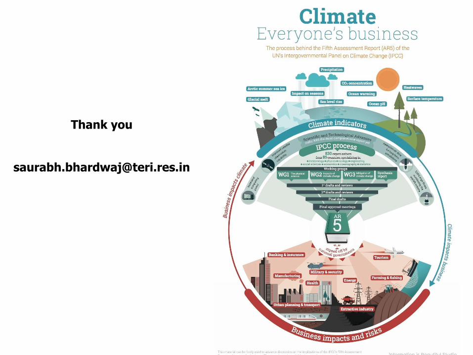
Climate Modelling: Basics Lecture at APN-TERI Student Seminar Teri University, 16 th Feb 2015 Saurabh Bhardwaj Associate Fellow Earth Science & Climate Change Division TERI [email protected]
Transcript of Climate Modelling: Basics Modelling: Basics Lecture at APN-TERI Student Seminar Teri University, ......

Climate Modelling:
Basics
Lecture at
APN-TERI Student Seminar
Teri University, 16th Feb 2015
Saurabh Bhardwaj
Associate Fellow
Earth Science & Climate Change Division
TERI
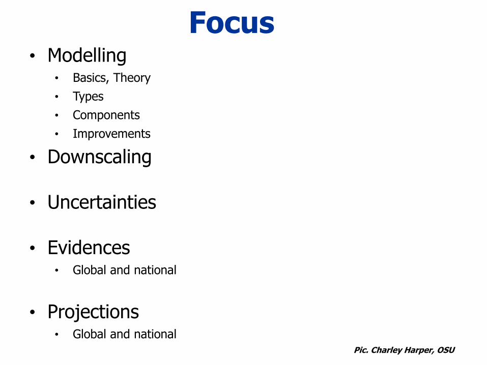
Focus • Modelling
• Basics, Theory
• Types
• Components
• Improvements
• Downscaling
• Uncertainties
• Evidences • Global and national
• Projections • Global and national
Pic. Charley Harper, OSU

Factors influencing climate
Incident solar radiation - variation with latitude
Closeness to large water bodies - distribution of land & water
Mountain barriers
Altitude
Ocean temperature and currents
Land cover
Atmospheric composition

The non-linear interaction among the components leads to climate variability at a range of spatial and temporal scales
Pic . NOAA
Interactions

Added
warming by
human
intervention
Review of Basics: Climate System
The non-linear interaction among the components leads to climate variability at a range of spatial and temporal scales

• The response of the climate system to this forcing agents is complicated by: feedbacks
the non-linearity of many processes
different response times of the different components to a given perturbation
• The only means available to calculate the response is by using numerical models of the climate system.
How do we quantify the response of the climate?

How do we define a Climate Model ?
“A climate model is a mathematical representation of the physical
processes that determine climate”
Why do we need Climate Models ?
To create an understanding of the climate processes.
To create plausible-scenarios, reflecting the current state of
scientific understanding.
To plan for the future.
“a simplified description, esp. a mathematical one, of a system or process, to assist calculations and predictions”
- dictionary
What is a Model ?

Models
Observations
Theory
Warner (2011) Numerical Weather and Climate Prediction. Cambridge University Press. McGuffie, K. and Henderson-Sellers, A. (2005) A Climate Modelling Primer. 3rd ed., Wiley.

Climate Modeling Climate model - an attempt to simulate many processes that produce climate
The simulation is accomplished by describing the climate system of basic physical laws.
Model is comprised of series of equations expressing these laws.
Climate models can be slow and costly to use, even on the faster computer, and the results can only be approximations.
The objective is to understand the processes and to predict the effects of changes and interactions.

Need for simplification The processes of climate system interact with each other, producing feedbacks, which in turn involves great deal of computation to simulate.
The solutions start from some “initialized” state and investigate the effects of changes in different components of climate system.
Boundary conditions – solar radiation or SST – set from obs. data, but since data itself aren‟t that complete, hence inherent uncertainty exists.
2 sets of simplifications
–Involving process
–Involving resolution of model in time and space
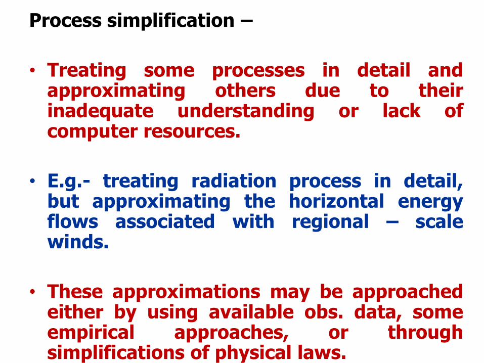
Process simplification –
• Treating some processes in detail and approximating others due to their inadequate understanding or lack of computer resources.
• E.g.- treating radiation process in detail, but approximating the horizontal energy flows associated with regional – scale winds.
• These approximations may be approached either by using available obs. data, some empirical approaches, or through simplifications of physical laws.
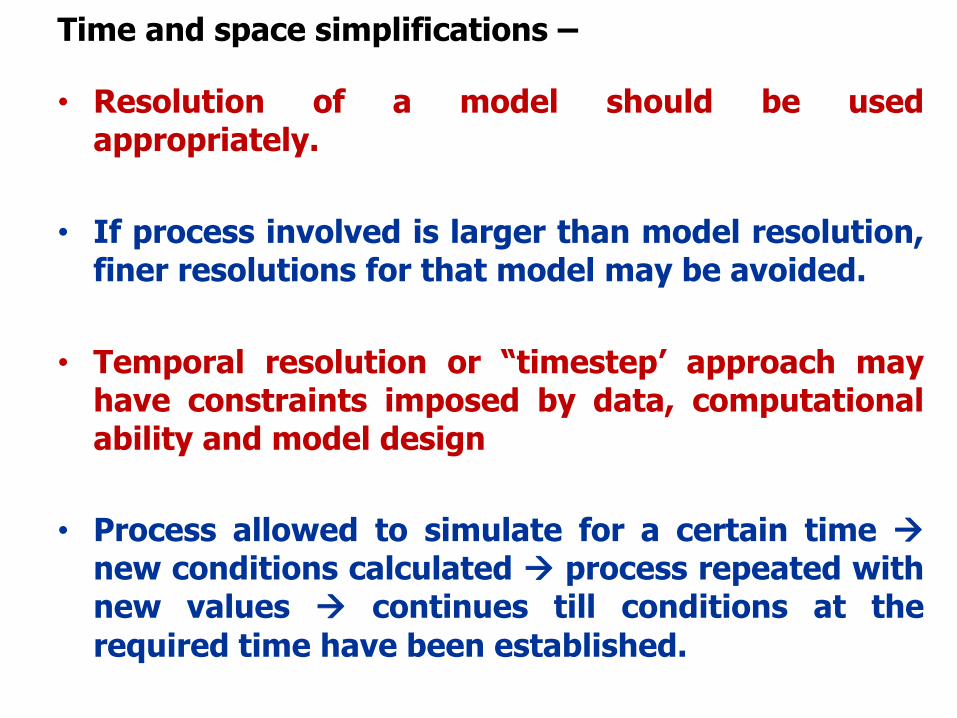
Time and space simplifications –
• Resolution of a model should be used appropriately.
• If process involved is larger than model resolution, finer resolutions for that model may be avoided.
• Temporal resolution or “timestep‟ approach may have constraints imposed by data, computational ability and model design
• Process allowed to simulate for a certain time new conditions calculated process repeated with new values continues till conditions at the
required time have been established.

Components of Climate models • Radiation – input and absorption of solar radiation and
emission of infrared radiation handled.
• Dynamics – horizontal movements of energy around the
globe (low to high lat.) and vertical movements
(convection etc.)
• Surface processes – inclusion of land/ocean/ice and the
resultant change in albedo, emissivity and surface-
atmosphere energy interactions.
• Resolution in both time and space – the time step of the
model and the horizontal and vertical scales resolved.

Framework for a Model
Source: MPI, Germany

McGuffie, K. and Henderson-Sellers, A. (2005) A Climate Modelling Primer. 3rd ed., Wiley.
Components of a weather/climate model
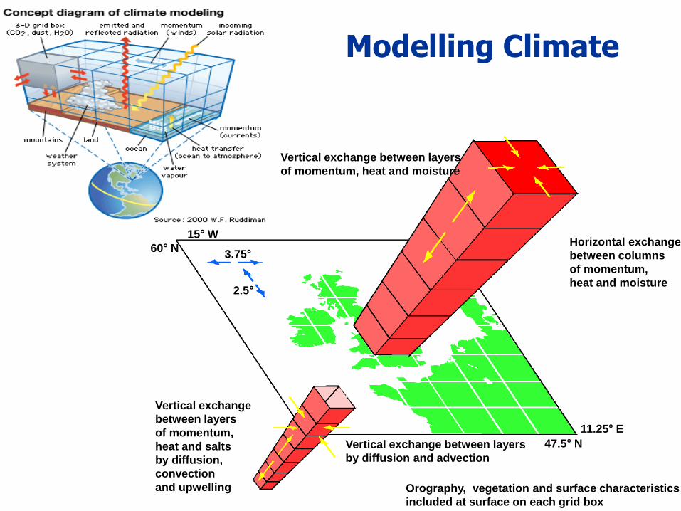
Vertical exchange between layers
of momentum, heat and moisture
Horizontal exchange
between columns
of momentum,
heat and moisture
Vertical exchange
between layers
of momentum,
heat and salts
by diffusion,
convection
and upwelling Orography, vegetation and surface characteristics
included at surface on each grid box
Vertical exchange between layers
by diffusion and advection
15° W
60° N 3.75°
2.5°
11.25° E
47.5° N
Modelling Climate

Numerical Solution: Time steps and Grid boxes
All the physical processes occurring in the climate system are resolved at
individual grid and the coupling occurs at these grids. Source: NASA

General Circulation Model:
Basic equations

Process of Model Simulation
Source: Goosse et al 2010
Generation of model source code
Supply of Initial and boundary conditions
Model Simulation

Types of climate Models 1. Energy Balance Models (EBMs)
zero or one dimensional
2. Radiative Convective (RC) Models one dimensional
3. Statistical Dynamical (SD) Models
two dimensional
4. Global Circulation Models (GCMs)
Three dimensional

Energy Balance Models (EBMs)
Zero or one-dimensional models predicting the variation of the surface (strictly sea level) temperature as a function of the energy balance of the earth with latitude.
Used to investigate sensitivity of climate systems to external changes and interpret results from complex models.
Radiative-Convective climate Models
Are 1-D with respect to altitude and compute the vertical (usually globally averaged) temperature profile by explicit modelling of radiative processes and „convective adjustment‟ which re-establishes a predetermined lapse rate.
RC models study the effects of changing atmospheric composition and investigate likely relative influences of different external and internal forcings.

Statistical Dynamical (SD) Models
Are 2-D models that deal explicitly with surface processes and dynamics in a zonally averaged framework and have vertically resolved atmosphere.
SD models used to make simulations of the chemistry of stratosphere and mesosphere.
Global Circulation Models (GCMs)
Where the 3-dimensional nature of the atmosphere and/or ocean is incorporated. Vertical resolution is generally finer than horizontal resolution. Includes AGCM, OGCM and the coupled AOGCM.
The resulting set of coupled non-linear equations are solved at each grid point using numerical techniques that use time step approach.
Atmospheric grid points ~ 2o-5o with time steps ~ 20-30 min. Vertical resolution ~ 6-50 levels (20 being typical).

Development of climate models
2000 2005
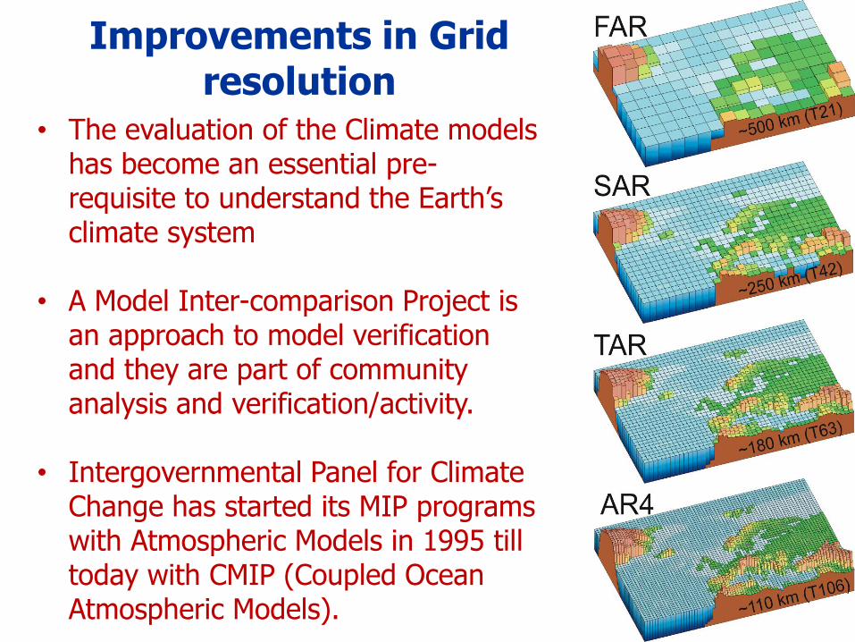
Improvements in Grid resolution
• The evaluation of the Climate models has become an essential pre-requisite to understand the Earth’s climate system
• A Model Inter-comparison Project is an approach to model verification and they are part of community analysis and verification/activity.
• Intergovernmental Panel for Climate Change has started its MIP programs with Atmospheric Models in 1995 till today with CMIP (Coupled Ocean Atmospheric Models).

Computational Capabilities and Needs
Improvements in computational capabilities have paved the
developments of atmospheric simulation capabilities
As an example, a 10-year global atmospheric simulation using a
state-of-art GCM can require several tens of hours of supercomputer
time approx 109 floating operations per second (1 Giga Flops)
Source: McGuffe, Henderson and sellers
Source: NCAR

1. Basic features of the general circulation of the
atmosphere (e.g. Hadley cell, mid-latitude jets)
2. Climatology (based on at least 5-10 years) e.g.
seasonal and monthly means.
3. Climate variability, e.g. behaviour of dominant
modes of inter-annual variability such as ENSO,
NAO.
4. Statistics of sub-seasonal variability e.g. monsoon
active/break cycles, storm-track characteristics
What can we expect to simulate?
What can we not expect to simulate?
1. The actual weather observed at individual
locations, at specific times.
2. A 100 % correlation with observations due to
inherent climate uncertainty. Hence, ensemble
approach is utilized.
3. Individual weather events. But climatological
statistics able to provide future frequency and
magnitude of such events.
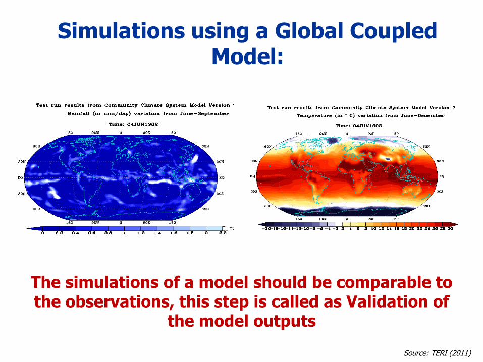
Simulations using a Global Coupled Model:
The simulations of a model should be comparable to the observations, this step is called as Validation of
the model outputs
Source: TERI (2011)

Typical data used to evaluate climate models
Re-analyses of the global circulation (ERA40, NCEP)
Synthesised climatologies e.g. precipitation
Satellite observations
In situ measurements
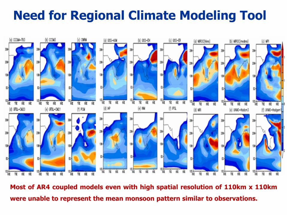
Need for Regional Climate Modeling Tool
Most of AR4 coupled models even with high spatial resolution of 110km x 110km
were unable to represent the mean monsoon pattern similar to observations.
Need for Regional Climate Modeling Tool
Most of AR4 coupled models even with high spatial resolution of 110km x 110km
were unable to represent the mean monsoon pattern similar to observations.
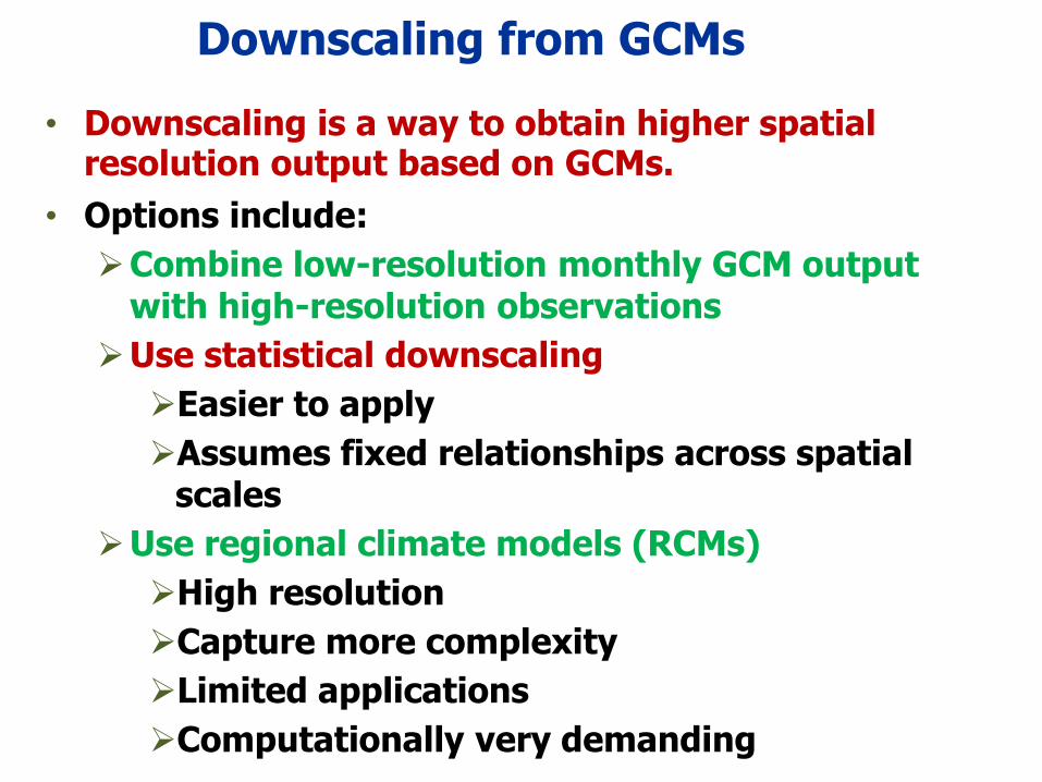
Downscaling from GCMs
• Downscaling is a way to obtain higher spatial resolution output based on GCMs.
• Options include:
Combine low-resolution monthly GCM output with high-resolution observations
Use statistical downscaling
Easier to apply
Assumes fixed relationships across spatial scales
Use regional climate models (RCMs)
High resolution
Capture more complexity
Limited applications
Computationally very demanding
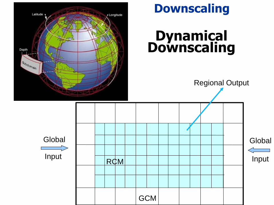
GCM
RCM Input
Global
Input
Global
Regional Output
Downscaling
Dynamical Downscaling

Regional Climate Models (RCMs)
• These are high resolution models that are “nested” within GCMs
• A common grid resolution is 50 km or lesser.
• RCMs are run with boundary conditions from GCMs
• They give much higher resolution output than GCMs
• Hence, much greater sensitivity to smaller scale factors such as mountains, lakes

Regional Modelling Product
RCM is able to capture the major features but overestimates the rainfall in
few regions.
Source: TERI (2011)

Lack of observations: poor model result
Annamalai, 2012

Uncertainties in Observation and Models
Turner and Annamalai, 2012

OBSERVATIONAL EVIDENCES
Temperature has risen
Warming is Unequivocal
IPCC, 2013, AR5 WG1
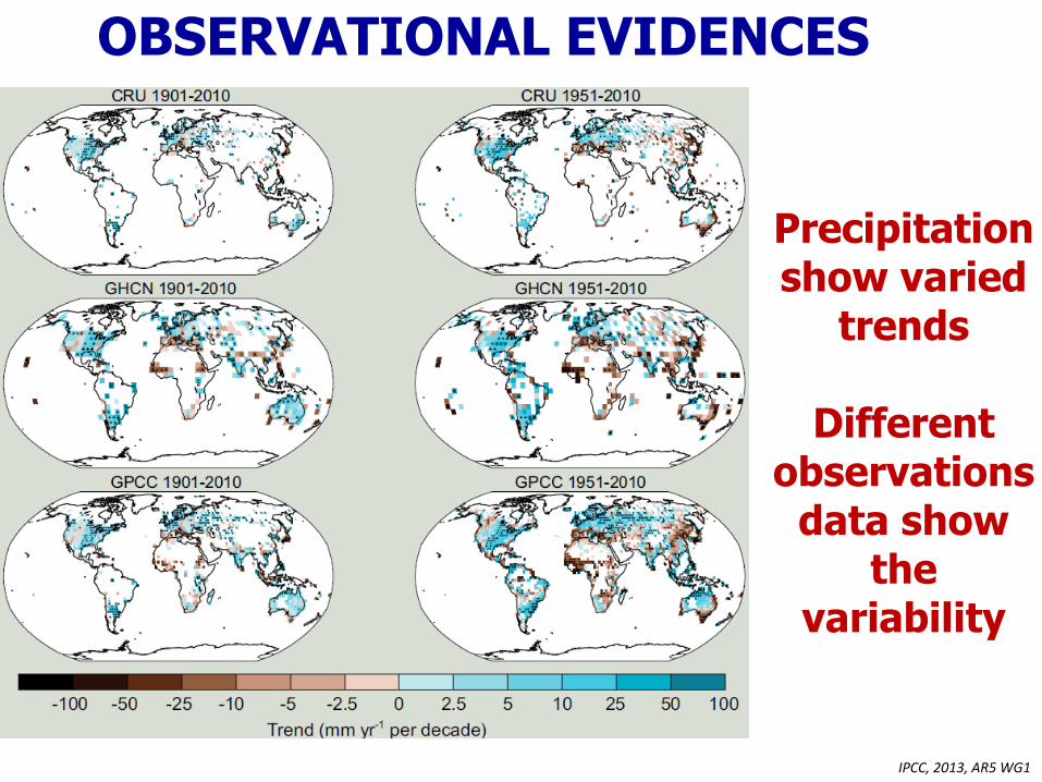
OBSERVATIONAL EVIDENCES
Precipitation show varied
trends
Different observations
data show the
variability
IPCC, 2013, AR5 WG1

S. Asia showing increasing
climate extremes

Decreasing cold nights and days
Increasing warm nights and days
IPCC, 2013, AR5 WG1

All India Mean Annual Temperature Anomalies
(1901-2007) (Base: 1961-1990)
Krishna Kumar, 2009

-6
-4
-2
0
2
4
6
-30
-25
-20
-15
-10
-5
0
5
10
15
20
25
30
18
75
18
80
18
85
18
90
18
95
19
00
19
05
19
10
19
15
19
20
19
25
19
30
19
35
19
40
19
45
19
50
19
55
19
60
19
65
19
70
19
75
19
80
19
85
19
90
19
95
20
00
20
05
20
10
31
Year ru
nn
ing m
ean
R
ain
fall
(% D
ep
artu
re)
YEAR
All India Rainfall (IITM ) and 31 Year Running Mean
All India Rainfall (IITM)
31 Year running mean
All-India monsoon season rainfall time series shows NO long term trends. It is marked by large year to year variations. There is a tendency of occurrence of more droughts in some epochs (for example, 1901-1930, 1961-1990).
Rajeevan, 2013
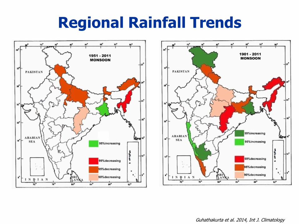
Regional Rainfall Trends
Guhathakurta et al. 2014, Int J. Climatology
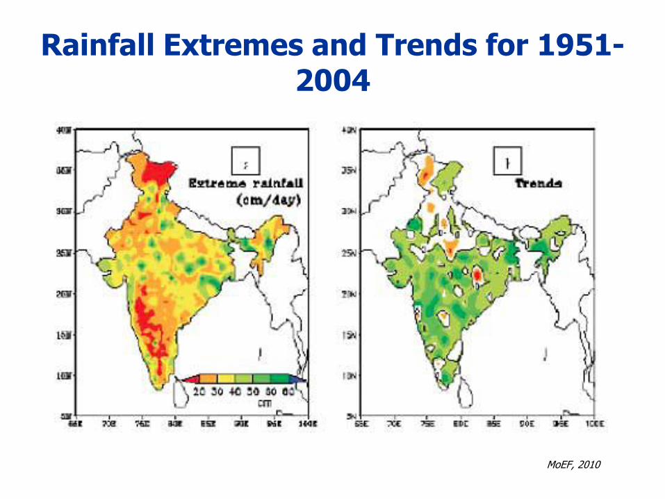
Rainfall Extremes and Trends for 1951-2004
MoEF, 2010

PROJECTIONS

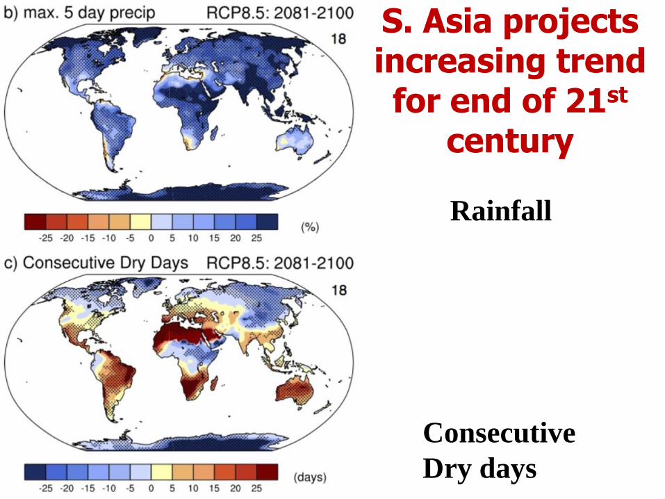
Rainfall
Consecutive
Dry days
S. Asia projects increasing trend for end of 21st
century

Difference in tropical easterly wave and cyclone statistics for 850 RV, between the 21C and 20C periods (21C – 20C), averaged over the three ensemble members before differencing. Mean intensity differences are only plotted where the track density is greater than 0.5 per month per unit area.
Source: Bengtsson et al. (2006) using TRACK
Track density
Mean intensity (10-5 s-1)
White lines: p-values < 5%
Projections for Tropical cyclones
Track density
Mean intensity (10-5 s-1)
SRES scenario A1B. Periods: 1961–90 (20th cent.) and 2071–2100 (21st cent.) Experiments from: Muller and Roeckner (2006)
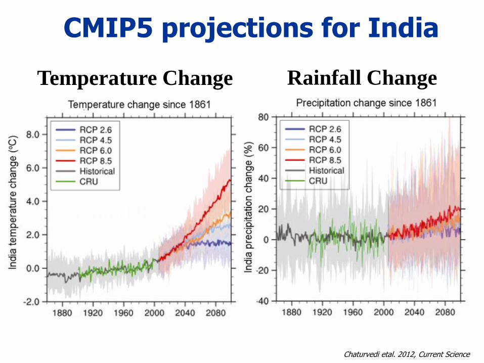
CMIP5 projections for India
Temperature Change Rainfall Change
Chaturvedi etal. 2012, Current Science
18 models

But how good are the models?
Temperature
Rainfall
Chaturvedi etal. 2012, Current Science
Observations Versus Ensemble mean for 1971-
1990
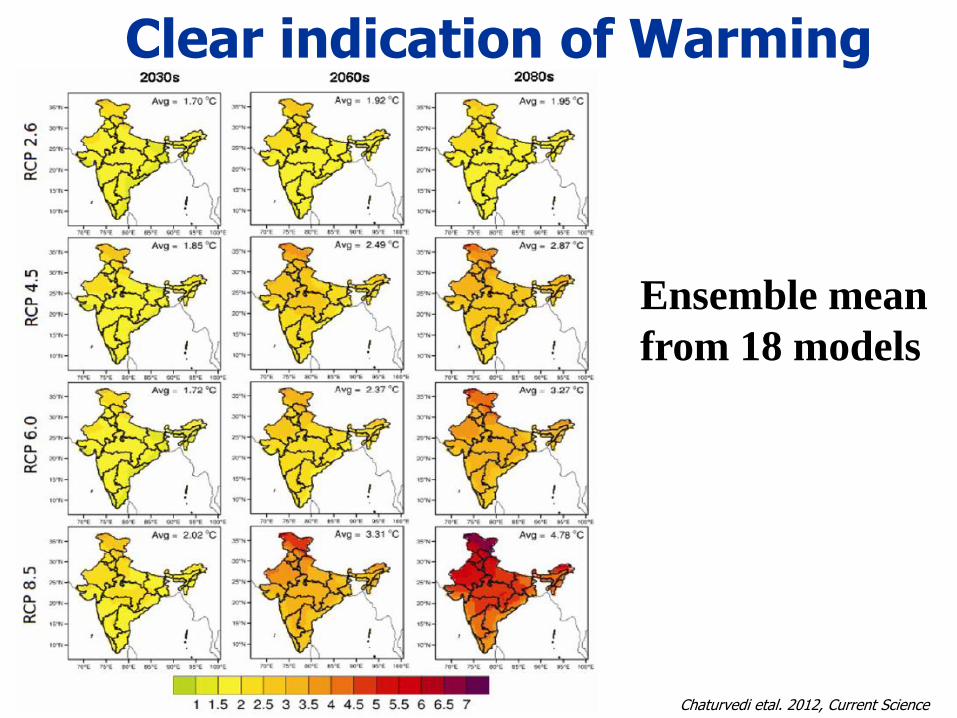
Clear indication of Warming
Chaturvedi etal. 2012, Current Science
Ensemble mean
from 18 models

% change in rainfall
Chaturvedi etal. 2012, Current Science
Ensemble mean
from 18 models
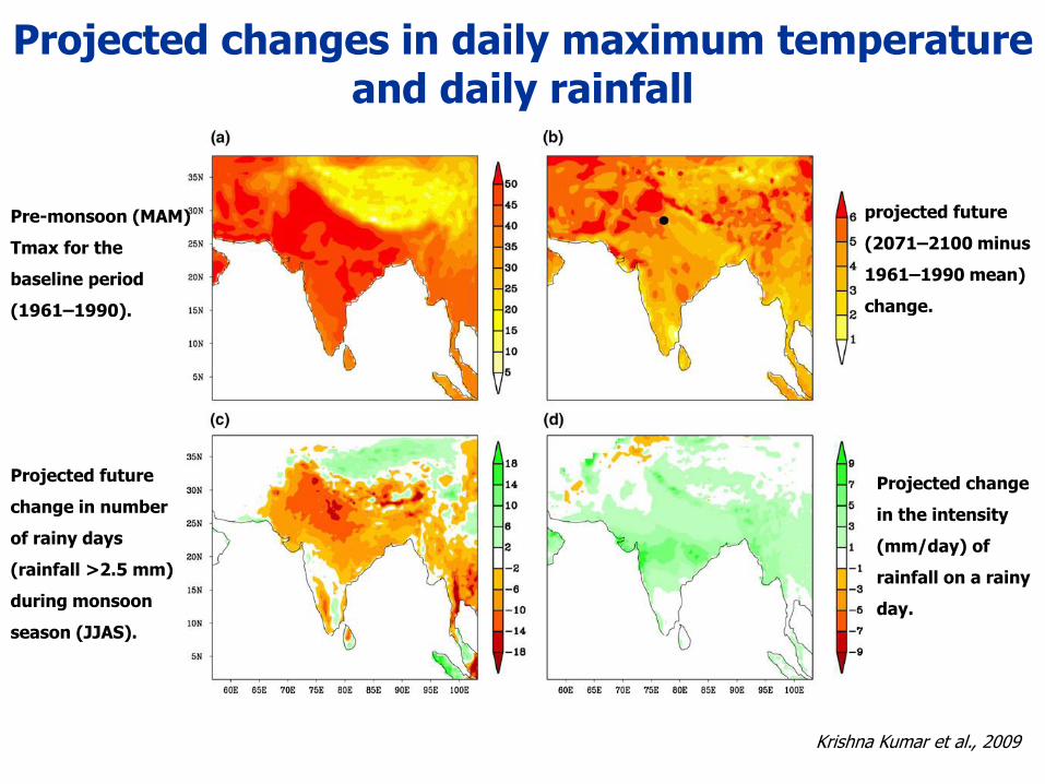
Krishna Kumar et al., 2009
Projected changes in daily maximum temperature and daily rainfall
Pre-monsoon (MAM)
Tmax for the
baseline period
(1961–1990).
projected future
(2071–2100 minus
1961–1990 mean)
change.
Projected future
change in number
of rainy days
(rainfall >2.5 mm)
during monsoon
season (JJAS).
Projected change
in the intensity
(mm/day) of
rainfall on a rainy
day.

Source-IMD