Climate change impacts in the Mediterranean resulting from a 2oC global temperature rise

A report for WWF

1 July 2005

C. Giannakopoulos, M. Bindi, M. Moriondo, P. LeSager and T. Tin

Published in July 2005 by WWF, the global conservation organization, Gland, Switzerland. Any reproduction in full or in part of this publication must mention the title and credit the above-mentioned publisher as the copyright owner. © text (2005) WWF. All rights reserved. The geographical designations in this report do not imply the expression of any opinion whatsoever on the part of WWF concerning the legal status of any country, territory, or area, or concerning the delimination of its frontiers or boundaries.

B

Climate change impacts in the Mediterranean resulting from a 2oC global temperature rise

Summary Tina Tin, Christos Giannakopoulos, Marco Bindi

The goal of the present study is to provide the first piece of the puzzle in

understanding the impacts of a 2°C global temperature rise on the Mediterranean region,

using high temporal resolution climate model output that has been made newly available.

The analysis has been based on the temperature, precipitation and wind daily outputs of

the HadCM3 model using the IPCC SRES A2 and B2 emission scenarios. The study is

focussed on the thirty-year period (2031-2060) centred on the time that global

temperature is expected to reach 2oC above pre-industrial levels, as defined by an

earlier companion study. Changes in both the mean (temperature, precipitation) and the

extremes (heatwaves, drought) under the different scenarios were assessed. The

impacts of these climatic changes on energy demand, forest fire, tourism and agriculture

were subsequently investigated either using existing numerical models or an expert-

based approach. Based on recent studies, the impacts on biodiversity, water resources

and sea level rise in the region were also discussed.

Our results show that a global temperature rise of 2°C is likely to lead to a

corresponding warming of 1-3 °C in the Mediterranean region. The warming is likely to

be higher inland than along the coast. The largest increase in temperature is expected to

take place in the summer, when extremely hot days and heatwaves are expected to

increase substantially, especially in inland and southern Mediterranean locations.

Under the A2 scenario, a drop in precipitation seems to be the dominant feature of

the future precipitation regime. Under the B2 scenario, rainfall increases in the northern

Mediterranean, particularly in winter. However, under both scenarios precipitation

decreases substantially in the summer in both the north and the south. In the south, the

reduction in precipitation extends year round. Longer droughts are shown to be common,

and are accompanied by shifts in timing. In terms of extremes, the number of dry days is

shown to increase while the number of wet and very wet days remains unchanged. This

C

can imply that when it rains it will rain more intensely and strongly, especially at certain

locations in the northern Mediterranean.

Based on the above climatic variables, we calculated the Canadian Fire Weather

Index to provide an indication of the forest fire risk under the future climate scenarios.

Under both A2 and B2 scenarios, fire risk is shown to increase nearly everywhere in the

Mediterranean region, especially in inland locations. The southern Mediterranean is at

risk of forest fire all year round. In the Iberian Peninsula, northern Italy and over the

Balkans, the period of extreme fire risk lengthens substantially. The only region that

shows little change in fire risk is in the southeastern Mediterranean.

Based on the same climatic data, we investigated the changes in agricultural crop

yields using a well-established numerical model. Our results show a general reduction in

crop yields (e.g. C3 and C4 summer crops, legumes, cereals, tuber crops). The southern

Mediterranean is likely to experience an overall reduction of crop yields due to the

change in climate. In some locations in the northern Mediterranean, the effects of

climate change and its associated increase in carbon dioxide may have little or small

positive impacts on yields, provided that additional water demands can be met. The

adoption of specific crop management options (e.g. changes in sowing dates or cultivars)

may help in reducing the negative responses of agricultural crops to climate change.

However, such options could require up to 40% more water for irrigation, which may or

may not be available in the future.

We calculated heating degree days (HDD) and cooling degree days (CDD) in order

to examine the change in heating and cooling requirements. Under both climate

scenarios, HDD decreases substantially in the northern Mediterranean and CDD

increases everywhere in the Mediterranean, especially in the south. This change can

potentially shift the peak in energy demand to the summer season with implications for

the need for additional energy capacity and increased stress on water resources.

Changes to tourism in the Mediterranean were examined through discussions with

experts and stakeholders. We expect that warmer northern European summers would

encourage northern Europeans to take domestic holidays and thus, not travel to the

Mediterranean. In addition, more frequent and intense heat waves and drought are likely

D

E

to discourage holidays in the Mediterranean in the summer. We expect that the

Mediterranean holiday season may shift to spring and autumn.

Based on results from existing studies, a global warming of 2°C and its associated

reduction in precipitation are expected to reduce surface runoff and water yields in the

Mediterranean region. In some countries, this could result in water demand exceeding

available water supply. In terms of biodiversity, climate change is likely to lead to shifts in

the distributions and abundances of species, potentially increasing the risks of extinction.

In addition, forest fires are expected to encourage the spread of invasive species which

in turn, have been shown to fuel more frequent and more intense forest fires.

Acknowledgments

The authors would like to thank Clare Goodess, Bob Bunce, Rafael Navarro, Antonio

Navarra, Riccardo Valentini, Michael Case and Lara Hansen for their comments on

earlier drafts of this report. Special thanks goes to Clare Goodess for her help during the

initial phase of the project, and to Mark New, Daniel Scott and Jacqueline Hamilton for

their helpful discussions.

F

Contents::

Page

C Summary

1 Climate change impacts on the Mediterranean resulting from a 2°C

temperature rise.

54 Impact of a 2° C global temperature rise on the Mediterranean

region: Agriculture analysis assessment.

G

H

Climate change impacts in the Mediterraneanresulting from a 2oC global temperature rise

Dr. Christos Giannakopoulos,

Dr. Philippe LeSager,

National Observatory of Athens, Athens, Greece

2

1. The Mediterranean region and climate: Basic issuesThe Mediterranean Region has many morphologic, geographical, historical and

societal characteristics, which make its climate scientifically interesting. In general, the

Mediterranean climate is characterised by mild wet winters and by warm to hot, dry

summers and may occur on the West Side of continents between about 30° and 40°

latitude.

The Mediterranean Sea, a marginal and semi-enclosed sea, is located on the

western side of a large continental area and is surrounded by Europe to the north, Africa

to the south, and Asia to the east. Its area, excluding the Black Sea, is about 2.5 million

km 2; its extent is about 3700 km in longitude, 1600 km in latitude and surrounded by 21

African, Asian and European countries. The average depth is 1500 m. with a maximum

depth of 5150 m in the Ionian Sea. The Mediterranean Sea is an almost completely

closed basin, being connected to the Atlantic Ocean through the narrow Gibraltar strait

(14.5 km wide, less than 300m deep at the sill). These morphologic characteristics are

rather unique. In fact, most of the other marginal basins have much smaller extent and

depth or they are connected through much wider openings to the open ocean. Moreover,

high mountain ridges surround the Mediterranean Sea on almost every side.

Furthermore, strong albedo differences exist in south-north directions (Bolle, 2003).

These characteristics have important consequences on air masses and atmospheric

circulation at the regional scale (e.g. Xoplaki 2002). The Mediterranean sea is an

important heat reservoir and source of moisture for surrounding land areas. It represents

an important source of energy and moisture for cyclone development and its complex

land topography plays a crucial role in steering air flow, so that energetic meso-scale

features are present in the atmospheric circulation.

Because of its latitude, the Mediterranean Sea is located in a transitional zone where

both mid-latitude and tropical variability is important and competes against each other.

The Mediterranean climate is exposed to the South Asian Monsoon in summer and the

Siberian high- pressure system in winter. The southern part of the region is mostly under

the influence of the descending branch of the Hadley cell, while the northern part is more

linked to the mid-latitude variability.

A further important characteristic of the Mediterranean Sea is the emergence of the

first highly populated and technologically advanced societies since, at least, 2000BC.

3

Because of the demographic pressure and exploitation of land for agriculture, the region

presents since ancient times important patterns of land-use change and important

anthropogenic effects on the environment, which are themselves interesting research

topics.

Nowadays, about 400 million people live in the countries around the Mediterranean

Sea. This densely populated area has large economic, cultural and demographic

contrasts. There are approximately 10-fold differences in GDP between the largest

economies of the European Union countries and small Middle East nations, and a 3 to 6-

fold difference in the GDP per-capita between Western European countries and the

other nations. Demographic trends are also quite different. European countries (also

including non EU nations) are close to a null growth and expected to stabilise or even

decrease their population, while North African and Asian countries are growing and are

expected to double their population by mid 21st century. In contrast to European

Countries, urbanisation for most African Nations is an ongoing process that is changing

the socio-economic structures of these regions. All these different trends are likely to

produce contrasts and conflicts in a condition of limited available resources. Moreover,

different level of services, of readiness to emergencies, technological and economical

resources, are likely to result in very different adaptation capabilities to environmental

and climate changes. Poorer societies with recently increased urbanisation are likely to

be critically vulnerable to weather extremes and incapable of adapting to changing

climate patterns. Hence the need is paramount for the best possible prediction of future

climate scenarios and descriptions of possible impacts and adaptation strategies.

2. Present trends of the Mediterranean climate2.1 Introduction

Instrumental data reveal significant trends of Mediterranean temperature and

precipitation at different time and space scales. For instance, during the last 50 years of

the 20th century large parts of the Mediterranean experienced winter and summer

warming. For the same period, precipitation over the Mediterranean decreased.

However, the statistical significance is low due to the large interannual variability. These

trends, however, differ across regions and periods under consideration showing

variability at a range of scales in response to changes in the direct radiative forcing and

variations in internal modes of the climate system. It is one of the main challenges for

future research to understand the physical processes and causes responsible for these

trends. They seem to be hemispheric to global (such as external forcings and changes in

the large-scale atmospheric circulation), anthropogenic as well as local/regional (such as

changes in earth surface and land use, orography).

2.2 Observed Temperature Trends over the Mediterranean Giorgi (2002) analysed the surface air temperature variability and trends over the

larger Mediterranean land-area for the 20th century based on gridded data of New et al.

(2000). He found a significant warming trend of 0.75°C per century, mostly from

contributions in the early and late decades of the century. Slightly higher values were

observed for winter and summer. Based on the same data, Jacobeit et al. (2003) found a

distinct summer warming for the 1969-1998 period. The structure of climate series can

differ considerably across regions showing variability at a range of scales in response to

changes in the direct radiative forcing and variations in internal modes of the climate

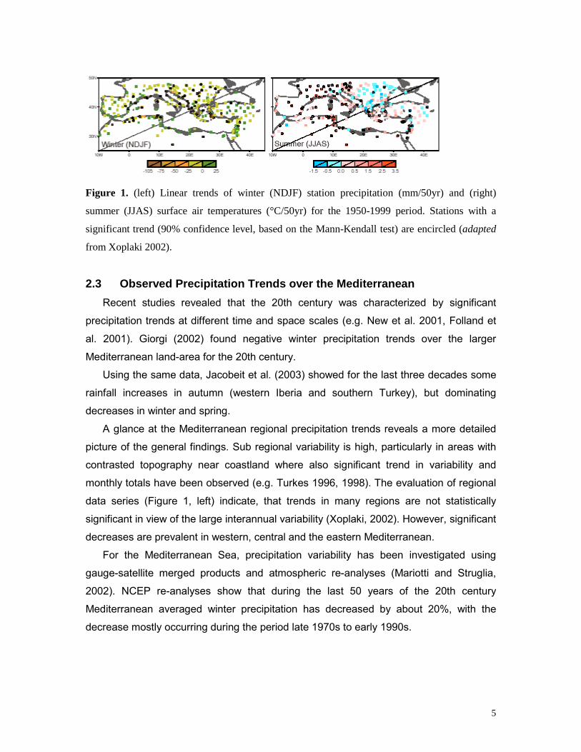
system (New et al. 2001; Hansen et al. 2001; Giorgi 2002). Figure 1 (right) presents the

linear trends of summer surface air temperatures (°C/50yr) for the period 1950-1999. It

also shows the stations, which experienced a significant trend.

A clear east-west differentiation in Mediterranean summer air temperature trends is

visible. Cooling, though mostly not significant, was experienced over the Balkans, and

parts of the eastern basin. In the other areas, there is a significant warming trend of up

to 3°C/50yr. However, the warming in these regions did not occur in a steady or

monotonic fashion. Over most of western Mediterranean for instance, it has been mainly

registered in two phases: from the mid-1920s to 1950 and from the mid-1970s onwards

(e.g. Brunet et al. 2001a, 2002, Galan et al. 2001). A glance at summer air temperature

trends for the 1900-1949 period reveals that warming, though less extreme than that in

1950-1999, was experienced in the western basin. A cooling trend over 1900-1949 was

only prevalent over Libya and Egypt. The trend of winter temperature over 1900-1949

indicates a general cooling in the central basin but a warming in the east and west. For

the 1950-1999 period, except for the eastern part, there was warming experienced.

Xoplaki et al. (2003) found a significant cooling trend of Mediterranean winter Sea

Surface Temperatures (SSTs) east of 20°E over the period 1950-1999, while the

western basin experienced warming.

4

5

Figure 1. (left) Linear trends of winter (NDJF) station precipitation (mm/50yr) and (right)

summer (JJAS) surface air temperatures (°C/50yr) for the 1950-1999 period. Stations with a

significant trend (90% confidence level, based on the Mann-Kendall test) are encircled (adapted

from Xoplaki 2002).

2.3 Observed Precipitation Trends over the MediterraneanRecent studies revealed that the 20th century was characterized by significant

precipitation trends at different time and space scales (e.g. New et al. 2001, Folland et

al. 2001). Giorgi (2002) found negative winter precipitation trends over the larger

Mediterranean land-area for the 20th century.

Using the same data, Jacobeit et al. (2003) showed for the last three decades some

rainfall increases in autumn (western Iberia and southern Turkey), but dominating

decreases in winter and spring.

A glance at the Mediterranean regional precipitation trends reveals a more detailed

picture of the general findings. Sub regional variability is high, particularly in areas with

contrasted topography near coastland where also significant trend in variability and

monthly totals have been observed (e.g. Turkes 1996, 1998). The evaluation of regional

data series (Figure 1, left) indicate, that trends in many regions are not statistically

significant in view of the large interannual variability (Xoplaki, 2002). However, significant

decreases are prevalent in western, central and the eastern Mediterranean.

For the Mediterranean Sea, precipitation variability has been investigated using

gauge-satellite merged products and atmospheric re-analyses (Mariotti and Struglia,

2002). NCEP re-analyses show that during the last 50 years of the 20th century

Mediterranean averaged winter precipitation has decreased by about 20%, with the

decrease mostly occurring during the period late 1970s to early 1990s.

2.4 Observed Daily Rainfall and Temperature Trends over the Mediterranean

Only few areas have been studied on a daily basis in the Mediterranean because

high quality data are rather scarce (e.g. De Luis et al. 2000). Difficulties exist in

determining trends of very rare events (e.g. Frei and Schär, 2001). One exception is the

dense daily rainfall data-base for the east of the Iberian Peninsula (Romero et al. 1998,

1999) which show successive drying in western Catalonia and central and western

Andalusia for the period 1964-1993. Brunetti et al. (2001ab) have found a negative trend

for the number of wet days and annual rainfall in Italy, while the heaviest events class

interval show a positive trends. Alpert et al. (2002), Brunetti et al. (2001ab), Goodess

and Jones (2002) also report on a tendency to more intense concentration of rainfall to

have occurred along some Mediterranean coastal areas, essentially Italy and Spain.

Similar results were found in two long observations in the north-eastern inland of Spain

(Ramos, 2001).

Over the western Mediterranean little change or even an increase of the day/night

temperature differences has been highlighted for the last 130 years (Brunet et al.

2001bc) and for the 20th century (Brunet et al. 1999, Abaurrea et al. 2001, Horcas et al.

2001). Maximum temperature increased at larger rates than minimum temperature. This

diurnal differential rate of warming, opposite to the observed on larger spatial scales, has

been mainly intensified during the second half of the 20th century.

3. Study overview

In this study, we conduct a “first-order” investigation on the impacts of a 2oC global

temperature rise in the Mediterranean basin. The analysis is based on the temperature,

precipitation and wind daily outputs of the HadCM3 model using two emission scenarios.

The study period is a thirty-year period (2031-2060) centred on the time of the 2oC global

temperature rise. Changes in both the mean (temperature, precipitation) and the

extremes (heatwaves, drought) under different future climate scenarios are assessed.

Subsequently, the impacts of these climatic changes on energy demand, forest fire,

tourism and agriculture are investigated. Impacts are examined using impact models

where such models exist in the literature (such as agriculture, forest fire, energy) or

using an expert-based approach when such models have not yet been developed (such

as for tourism). The likely magnitudes of uncertainties and the sensitivity of HadCM3

6

7

relative to other climate models are discussed. Based on recent work in the published

literature, we also examine the consequences of such a change in climate on water

availability, biodiversity and sea level rise in the region. The goal of the present study is

to provide the first piece of the puzzle in understanding the impacts of a 2°C global

temperature rise on the Mediterranean region, using high temporal resolution climate

model output that has been made newly available. Although only a single climate model

has been used in this study, we believe that our results are representative of average or

conservative values within the range of similar estimates from currently available climate

models. This arises from the use of a model of average sensitivity to investigate a period

during which there is reasonable agreement among models (Section 4.3). Before larger

scale and more comprehensive multi-model, multi-year studies are undertaken, such a

first-order study can provide invaluable information in the planning of future research or

policy directions.

Within the context of ongoing studies, the present study is an extension of the 3-year

European project MICE (Modeling the Impacts of Climate Extremes), which has involved

8 institutes since 2002 in analyzing the occurrence of extremes in climate models and

quantifying the impacts of climate extremes on selected European environments, using

the same climate model output from HadCM3 (Giannakopoulos and Palutikof, 2005;

Palutikof, 2004). MICE has now been superseded by the Integrated EU project

ENSEMBLES (involving 72 European research Institutes) , which compliments MICE by

providing probabilistic estimates of climatic risk and by characterising the level of

confidence in future climate scenarios through ensemble integrations of climate models

(Hewitt and Griggs, 2004).

4. Data and methods 4.1 Time of 2oC global temperature rise

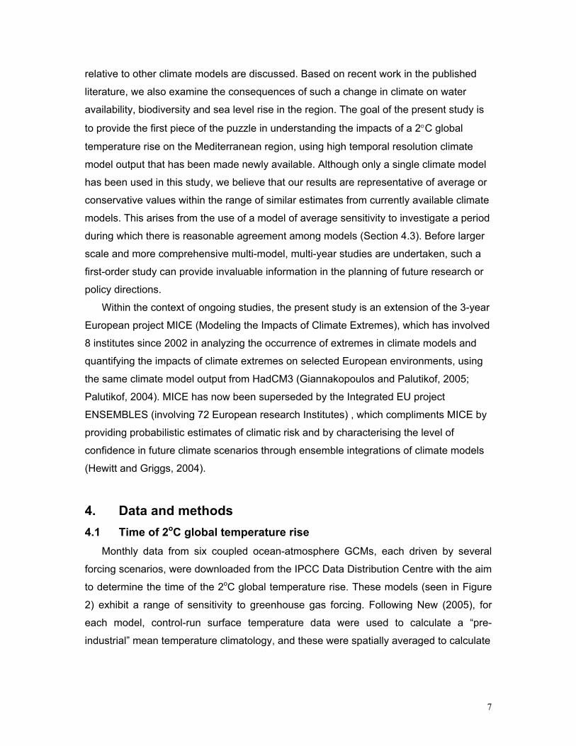
Monthly data from six coupled ocean-atmosphere GCMs, each driven by several

forcing scenarios, were downloaded from the IPCC Data Distribution Centre with the aim

to determine the time of the 2oC global temperature rise. These models (seen in Figure

2) exhibit a range of sensitivity to greenhouse gas forcing. Following New (2005), for

each model, control-run surface temperature data were used to calculate a “pre-

industrial” mean temperature climatology, and these were spatially averaged to calculate

8

a global mean pre-industrial surface temperature. For each climate change simulation,

the global temperature fields were spatially averaged to calculate time-series of global

mean annual temperature, which were then differenced from the “pre-industrial” global

mean temperature. The resulting global mean temperature-anomaly series were then

smoothed with a 21-year moving average, and the date at which the 21-year mean

global temperature anomaly exceeded 2°C above pre-industrial levels was taken as the

time of 2°C global temperature change.

The time at which the simulated global mean temperature exceeds the control run

global mean by 2°C ranges from between 2026 and 2060. The inter-model spread for a

single scenario (e.g. B2) is nearly as large as the total spread; however, there is a

tendency for the scenarios with greater accumulated radiative forcing (e.g. A2) to exhibit

a greater rate of warming, and an earlier year of 2oC global rise.

Figure 2. Global mean annual temperature anomalies relative to control climatology, smoothed with a 21-year moving average. Vertical lines indicate the range in time at which the 21-year global meantemperature anomaly exceeds +2°C. Figures on the right show the time at which the 21-year mean globaltemperature anomaly exceeds +2°C for each GCM-scenario combination (adapted from New, 2005).

9

300

400

500

600

700

800

900

1000

1990 2000 2010 2020 2030 2040 2050 2060 2070 2080 2090 2100

CO

2 Con

cetra

tion

(ppm

)A1B A1T A1FI A2 B1 B2 IS92a

1.0

3.0

5.0

7.0

9.0

1990 2000 2010 2020 2030 2040 2050 2060 2070 2080 2090 2100

Rad

iativ

e Fo

rcin

g (W

/m2 )

A1B A1T A1FI A2 B1 B2 IS92agsIS92agg

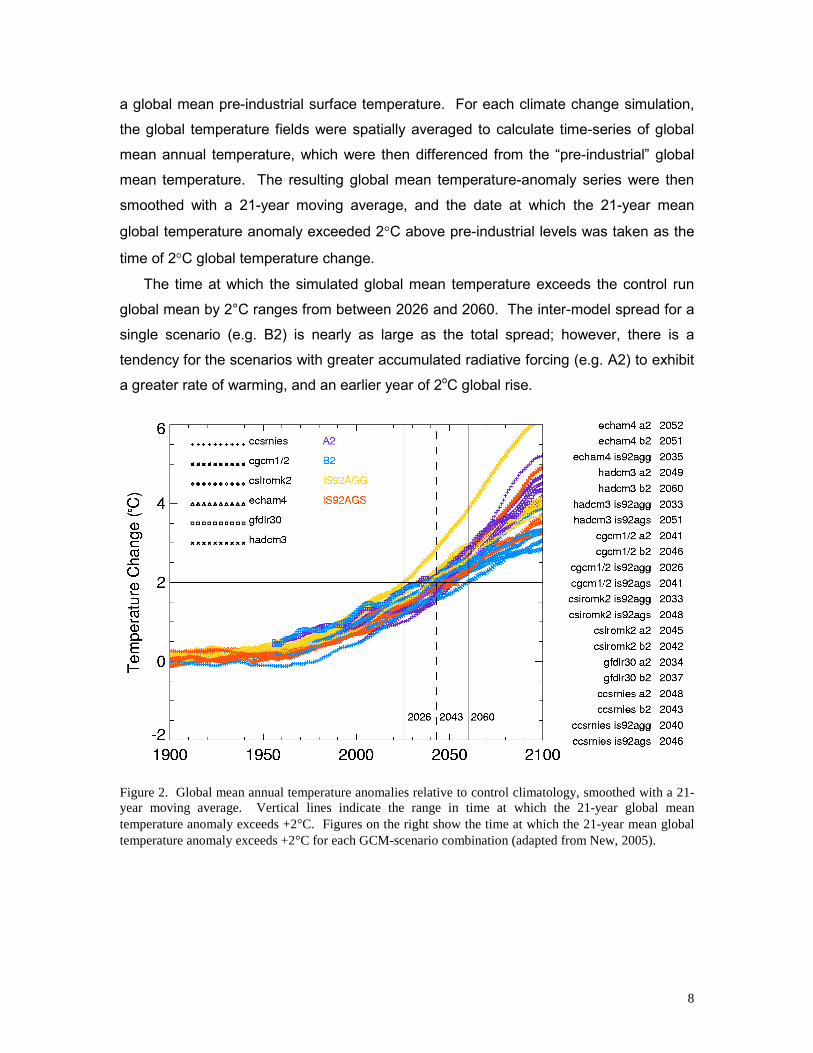
Figure 3. Estimated concentrations of CO2 and globally averaged increase in radiative forcing from allgreenhouse gases and aerosols (relative to preindustrial levels) arising from various IPCC emissionsscenarios. Scenarios used in this study are in bold. Data from Appendix II of IPCC (2001b). Adapted fromNew (2005).

We focused on the results from 2 IPCC forcing scenarios, namely A2 and B2. As

described in Nakicenovic et al. (2000), the A2 storyline and scenario family describes a

very heterogeneous world. The underlying theme is self-reliance and preservation of

local identities. Fertility patterns across regions converge very slowly, which results in

continuously increasing global population. Economic development is primarily regionally

oriented and per capita economic growth and technological change are more

10

fragmented and slower than in other storylines. The B2 storyline and scenario family

describes a world in which the emphasis is on local solutions to economic, social, and

environmental sustainability. It is a world with continuously increasing global population

at a rate lower than A2 and intermediate levels of economic development. While the

scenario is also oriented toward environmental protection and social equity, it focuses on

local and regional levels. The B2 scenario family is based on the long-term UN Medium

1998 population projection of 10.4 billion by 2100. The A2 scenario family is based on a

high population growth scenario of 15 billion by 2100 that assumes a significant decline

in fertility for most regions and stabilization at above replacement levels. It falls below

the long-term 1998 UN High projection of 18 billion.

The radiative forcing under the two scenarios are less divergent for the expected

period of 2°C global temperature rise (2026-2060, Fig. 2) than for the latter part of the

century (Fig. 3).

4.2 The HadCM3 ocean-atmosphere coupled GCMWe have used daily output data from a coupled atmosphere-ocean general

circulation model (GCM) HadCM3, consisting of an atmospheric GCM coupled to an

ocean GCM. HadCM3 is a coupled atmosphere-ocean GCM, developed at the Hadley

Centre and described by Gordon et al (2000) and Pope et al (2000). Unlike earlier

atmosphere-ocean GCMs at the Hadley Centre and elsewhere, HadCM3 does not need

flux adjustment (additional "artificial" heat and freshwater fluxes at the ocean surface) to

produce a good simulation. The higher ocean resolution of HadCM3 is a major factor in

this. HadCM3 has been run for over a thousand years, showing little drift in its surface

climate. The control run is basically the GCM being run for 240 years at 1961-1990

atmospheric concentrations. Any variation in the control run is, hopefully, due solely to

natural variability. The last 30 years of the control run, 1961-1990, are used here as

reference for comparison with future predictions. The control run is unforced and thus

common to any scenario that may apply after 1990.

The atmospheric component of HadCM3 has 19 levels with a horizontal resolution of

2.5° of latitude by 3.75° of longitude, which produces a global grid of 96 x 73 grid cells.

This is equivalent to a surface resolution of about 417 km x 278 km at the Equator,

reducing to 295 km x 278 km at 45° of latitude (comparable to a spectral resolution of

T42). Thus the model geography is much simpler than the real-world geography. As an

example, only five grid boxes cover the UK and one land grid box represents continental

11

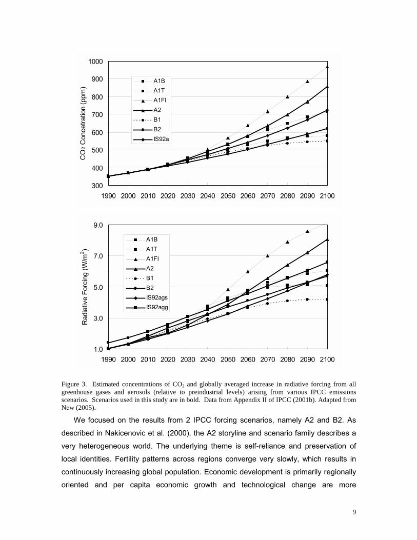
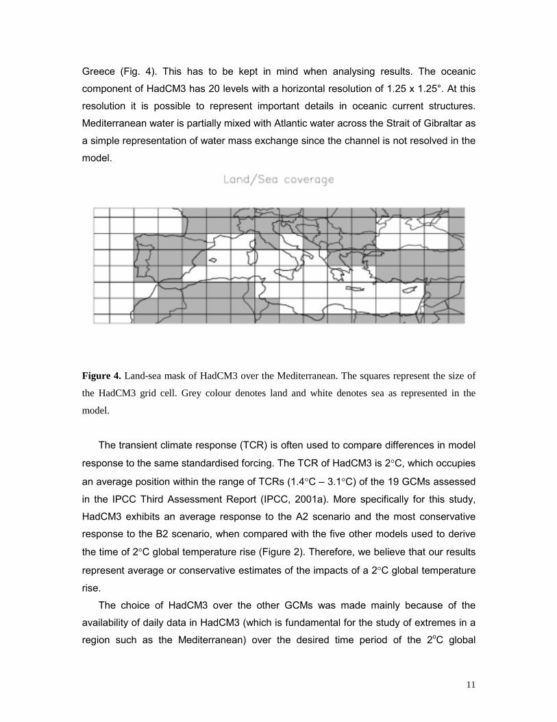
Greece (Fig. 4). This has to be kept in mind when analysing results. The oceanic

component of HadCM3 has 20 levels with a horizontal resolution of 1.25 x 1.25°. At this

resolution it is possible to represent important details in oceanic current structures.

Mediterranean water is partially mixed with Atlantic water across the Strait of Gibraltar as

a simple representation of water mass exchange since the channel is not resolved in the

model.

Figure 4. Land-sea mask of HadCM3 over the Mediterranean. The squares represent the size of

the HadCM3 grid cell. Grey colour denotes land and white denotes sea as represented in the

model.

The transient climate response (TCR) is often used to compare differences in model

response to the same standardised forcing. The TCR of HadCM3 is 2°C, which occupies

an average position within the range of TCRs (1.4°C – 3.1°C) of the 19 GCMs assessed

in the IPCC Third Assessment Report (IPCC, 2001a). More specifically for this study,

HadCM3 exhibits an average response to the A2 scenario and the most conservative

response to the B2 scenario, when compared with the five other models used to derive

the time of 2°C global temperature rise (Figure 2). Therefore, we believe that our results

represent average or conservative estimates of the impacts of a 2°C global temperature

rise.

The choice of HadCM3 over the other GCMs was made mainly because of the

availability of daily data in HadCM3 (which is fundamental for the study of extremes in a

region such as the Mediterranean) over the desired time period of the 2oC global

12

temperature rise. Output from regional models would provide higher spatial resolution

but are not available for this period. A study that uses one model, with one ensemble,

only gives one picture of the climate response to a given forcing scenario. In theory,

using more models and more ensembles should give more statistically reliable results. In

practice, this can be misleading because the models may all use the same forcing

model, which can influence the projected climate response more than the emissions

scenario. Moreover, there may be insufficient models/ensembles to give a representative

mean projected climate response so that the climate response can be biased towards

the least representative (probably the worst) model. Under these cases, it is arguably

better to use a single model that generally gives a good overall representation of current

climate and extremes and where you understand its weaknesses, which is what was

done in the present study. In addition, model comparison studies have shown that

results from different models for the study period agree with one another fairly well, while

most of the divergence takes place in the latter part of the century (2070-2100) (IPCC,

2001a).

4.3 MethodologyIn order to determine the changes in the Mediterranean climate and their impacts as

a result of a 2°C global temperature rise, our study focused on the period of 2031-2060

(Fig. 2).

The meteorological data from HadCM3 model have been processed to produce

yearly characteristics such as the maximum length of the drought, the number of

summer days, or percentile values. These parameters have been averaged over the

1961-1990 (reference or control period) and the 2031-2060 periods. The results for the

two periods are then compared.

Both scenarios (A2 and B2) give similar results, except in few cases specifically

noted hereafter. The two scenarios bring more differences in the 2070-2100 period,

which is not the period of interest here.

Precipitation, and maximum (daytime), minimum (night- time), and mean

temperatures have been examined. Wind (max and mean) do not show any significant

changes and will not be discussed here.

13

4.4 UncertaintiesMost of our findings in this study will be subject to uncertainties corresponding to

more than one of the classes below:

1. Incomplete or imperfect observation. This is a joint property of the system being

studied (e.g., Earth’s climate, crop responses to climate) and our ability to measure it.

2. Incomplete conceptual frameworks, e.g., models that do not include all relevant

processes, etc.

3. Inaccurate prescriptions of known processes, e.g., poor parameterizations etc.

4. Chaos. This is a property of the system (e.g., Earth’s climate, crop responses to

climate) being studied.

5. Lack of predictability. Some aspects of societal prediction are much less amenable to

prediction than others. For example, in considering new technologies, uncertainties

associated with rates of market penetration of new technologies are smaller than those

associated with rates of onset of the new technologies themselves.

In seeking to characterize uncertainty, the concept of the ‘uncertainty cascade’,

shown below, has been developed (IPCC, 2001b). This starts with different socio-

economic assumptions that affect projections of GHG emissions, and flows through

differing potential emission scenarios and ranges of GHG concentrations, radiative

forcing, and climate system responses and feedbacks. These in turn affect the

estimation of the range of potential impacts, and the consideration of adaptation and

mitigation responses and policies.

Figure 5. The concept of “uncertainty cascade” in climate change impact analyses. Adapted from

IPCC (2001b).

14

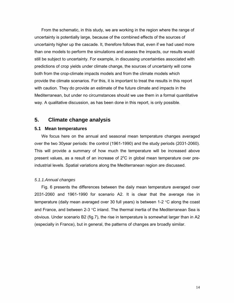
From the schematic, in this study, we are working in the region where the range of

uncertainty is potentially large, because of the combined effects of the sources of

uncertainty higher up the cascade. It, therefore follows that, even if we had used more

than one models to perform the simulations and assess the impacts, our results would

still be subject to uncertainty. For example, in discussing uncertainties associated with

predictions of crop yields under climate change, the sources of uncertainty will come

both from the crop-climate impacts models and from the climate models which

provide the climate scenarios. For this, it is important to treat the results in this report

with caution. They do provide an estimate of the future climate and impacts in the

Mediterranean, but under no circumstances should we use them in a formal quantitative

way. A qualitative discussion, as has been done in this report, is only possible.

5. Climate change analysis5.1 Mean temperatures

We focus here on the annual and seasonal mean temperature changes averaged

over the two 30year periods: the control (1961-1990) and the study periods (2031-2060).

This will provide a summary of how much the temperature will be increased above

present values, as a result of an increase of 2oC in global mean temperature over pre-

industrial levels. Spatial variations along the Mediterranean region are discussed.

5.1.1.Annual changes

Fig. 6 presents the differences between the daily mean temperature averaged over

2031-2060 and 1961-1990 for scenario A2. It is clear that the average rise in

temperature (daily mean averaged over 30 full years) is between 1-2 °C along the coast

and France, and between 2-3 °C inland. The thermal inertia of the Mediterranean Sea is

obvious. Under scenario B2 (fig.7), the rise in temperature is somewhat larger than in A2

(especially in France), but in general, the patterns of changes are broadly similar.

15

Figure 6. Difference between the daily mean temperature averaged over 2030-2060 and over 1961-1990,for scenario A2.

Figure 7. As Fig. 6 but for scenario B2.

Figs. 8 and 9 show also the same pattern as Figure 6 but for the daily maximum (Tmax)

and minimum temperatures (Tmin) respectively. It is worth noting that the average rise is

slightly larger for Tmax than for Tmin. In the figures, this is particularly evident in the

Iberian Peninsula.

16

Figure 8. As Fig. 6 but for the daily maximum temperature.

Figure 9. As Fig. 6 but for the daily minimum temperature.

17

5.1.2 Seasonal changes

Figs. 10, 11 & 12 present the variations in mean (Tmean), maximum (Tmax), and

minimum (Tmin) temperatures, respectively, for each of the four seasons, as projected

under the A2 scenario.

Figure 10. As Fig. 6 but for each season (Winter=DJF, Spring=MAM, Summer=JJA, Fall=SON).

For Tmean (Fig. 10), the rise occurs mainly in summer, when it reaches 4 °C inland

on average. Fall is the second season to get warmer, with temp rises above the 2 °C

average. Winter is likely to be uniformly warmer by 1-2 °C. Spring experiences the

average 2 °C increase, except in the north-western part of the region, where the

warming is less.

Tmin (Fig. 11) features the same seasonal variation, with a slightly smaller increase

in summer than Tmean.

18

Figure 11. As Fig. 10 but for the daily minimum temperature.

Tmax (Fig. 12) features the same seasonal variation, with a rise notably larger than

Tmean in summer and slightly larger in fall.

19

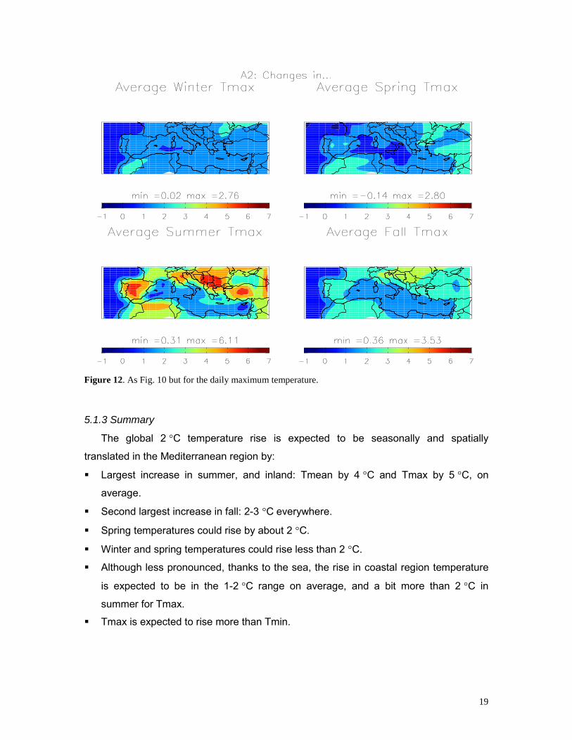
Figure 12. As Fig. 10 but for the daily maximum temperature.

5.1.3 Summary

The global 2 °C temperature rise is expected to be seasonally and spatially

translated in the Mediterranean region by:

� Largest increase in summer, and inland: Tmean by 4 °C and Tmax by 5 °C, on

average.

� Second largest increase in fall: 2-3 °C everywhere.

� Spring temperatures could rise by about 2 °C.

� Winter and spring temperatures could rise less than 2 °C.

� Although less pronounced, thanks to the sea, the rise in coastal region temperature

is expected to be in the 1-2 °C range on average, and a bit more than 2 °C in

summer for Tmax.

� Tmax is expected to rise more than Tmin.

20

5.2 High temperatures5.2.1 Summer days

The increase in the number of summer days, defined as the number of days when

Tmax exceeds 25oC, is from 2-to-6 weeks (Fig. 13 top). This is translated to about one

additional month of summer days on average.

� Large increases are found in Central Mediterranean Region (i.e. Crete,

Peloponnese, South Greece, Sicily), North Adriatic, and inland (within Maghreb,

Spain, Turkey, South of France and the Balkans). In this group, the largest increase

seems to occur in Crete with an additional 7 weeks of summer and the smallest in

the Maghreb with an additional 3-5 weeks of summer.

� On the other hand, the coastal regions of the western Mediterranean, the Black Sea

and the Middle East is expected to have the smallest increases with only 2-3

additional weeks of summer.

� It is expected that there will be, on average, one additional summer month

everywhere inland, as well as in the central Mediterranean coastal region, and about

half a month on all other coastal regions except the central Mediterranean Region.

5.2.2 Hot days

The pattern in the number of hot days, defined as the number of days with Tmax> 30 °C

(Fig. 13 bottom) is somewhat different from the pattern of the number of summer days.

The increase is from 2 weeks along the coast to 5-6 weeks inland (within Spain, Turkey,

South of France, the Balkans and in the Maghreb) indicating the role the Mediterranean

Sea exerts in preventing too hot days.

5.2.3 Summary

According to our study, there exist four types of regions:

� Inland: on average one additional month of hot days, and also one additional month

of summer days.

� Along the coasts outside Central Mediterranean region: 1-3 weeks of additional hot

days, and 2-3 weeks of additional summer days.

� The coastal regions in Central and Eastern Mediterranean region are expected to

have only few additional hot days (like the other coastal regions), but one additional

month of summer days, as in the continental part of the Mediterranean. Crete is the

21

perfect example: no change in the number of hot days, but an average of 7 additional

weeks of summer days.

It looks as if the Mediterranean Sea moderates temperature increases in the coastal

areas so while more summer days are forecast, few of these days will be on the hot

side.

Figure 13. Differences in the number of summer (top) and hot (bottom) days between control and futureperiod for scenario A2.

5.2.4 Tropical nights

The number of tropical nights, defined as the number of nights with Tmin > 20 °C

(fig.14) increases by about a month almost everywhere. Only regions well within land are

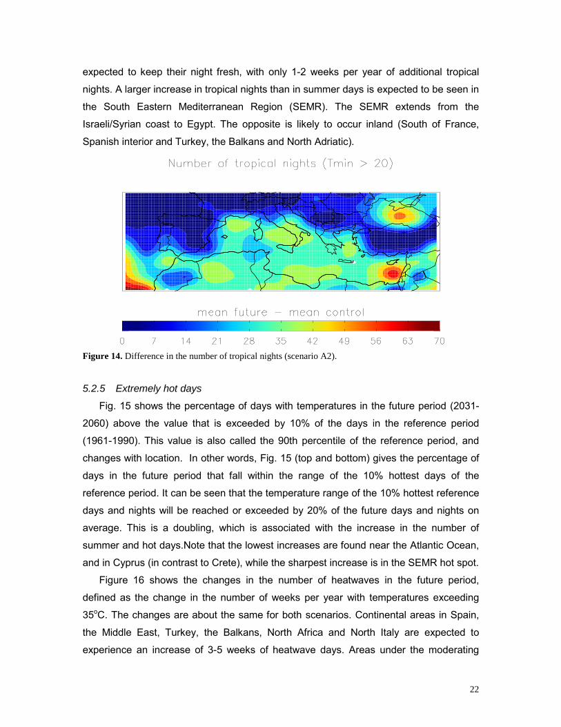
22

expected to keep their night fresh, with only 1-2 weeks per year of additional tropical

nights. A larger increase in tropical nights than in summer days is expected to be seen in

the South Eastern Mediterranean Region (SEMR). The SEMR extends from the

Israeli/Syrian coast to Egypt. The opposite is likely to occur inland (South of France,

Spanish interior and Turkey, the Balkans and North Adriatic).

Figure 14. Difference in the number of tropical nights (scenario A2).

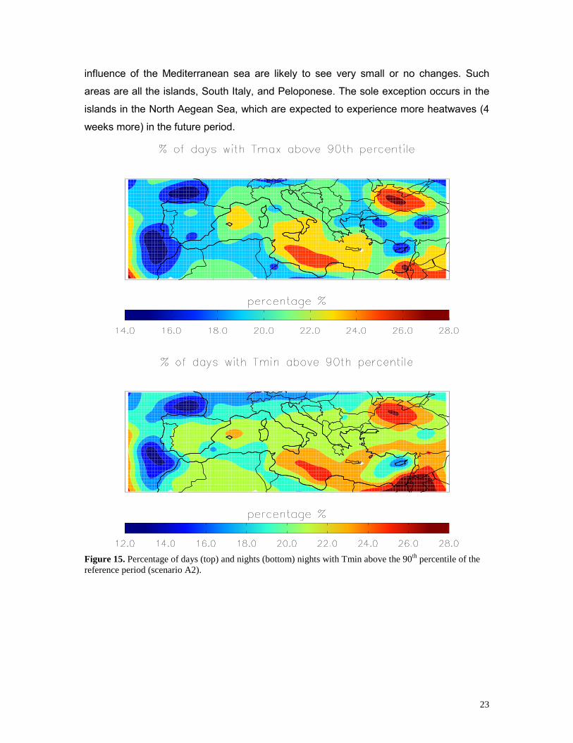
5.2.5 Extremely hot days

Fig. 15 shows the percentage of days with temperatures in the future period (2031-

2060) above the value that is exceeded by 10% of the days in the reference period

(1961-1990). This value is also called the 90th percentile of the reference period, and

changes with location. In other words, Fig. 15 (top and bottom) gives the percentage of

days in the future period that fall within the range of the 10% hottest days of the

reference period. It can be seen that the temperature range of the 10% hottest reference

days and nights will be reached or exceeded by 20% of the future days and nights on

average. This is a doubling, which is associated with the increase in the number of

summer and hot days.Note that the lowest increases are found near the Atlantic Ocean,

and in Cyprus (in contrast to Crete), while the sharpest increase is in the SEMR hot spot.

Figure 16 shows the changes in the number of heatwaves in the future period,

defined as the change in the number of weeks per year with temperatures exceeding

35oC. The changes are about the same for both scenarios. Continental areas in Spain,

the Middle East, Turkey, the Balkans, North Africa and North Italy are expected to

experience an increase of 3-5 weeks of heatwave days. Areas under the moderating

23

influence of the Mediterranean sea are likely to see very small or no changes. Such

areas are all the islands, South Italy, and Peloponese. The sole exception occurs in the

islands in the North Aegean Sea, which are expected to experience more heatwaves (4

weeks more) in the future period.

Figure 15. Percentage of days (top) and nights (bottom) nights with Tmin above the 90th percentile of thereference period (scenario A2).

24

Figure 16. Difference in the number of heatwaves (i.e. weeks with Tmax>35oC) under A2 scenariobetween the two periods.

5.3 Low temperaturesFig. 17 reveals that the number of frost nights, defined as the number of nights

with Tmin < 0 °C, falls by 1-2 weeks along the coast, and up to a month inland. The

number of very cold nights (Tmin < -5 °C) is not shown but it also has a decreasing

trend (though not as strong).

Figure 17. Difference in the number of frost nights (scenario A2).

25

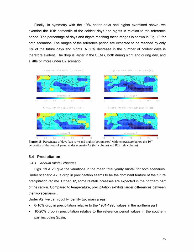
Finally, in symmetry with the 10% hotter days and nights examined above, we

examine the 10th percentile of the coldest days and nights in relation to the reference

period. The percentage of days and nights reaching these ranges is shown in Fig. 18 for

both scenarios. The ranges of the reference period are expected to be reached by only

5% of the future days and nights. A 50% decrease in the number of coldest days is

therefore evident. The drop is larger in the SEMR, both during night and during day, and

a little bit more under B2 scenario.

Figure 18. Percentage of days (top row) and nights (bottom row) with temperature below the 10th

percentile of the control years, under scenario A2 (left column) and B2 (right column).

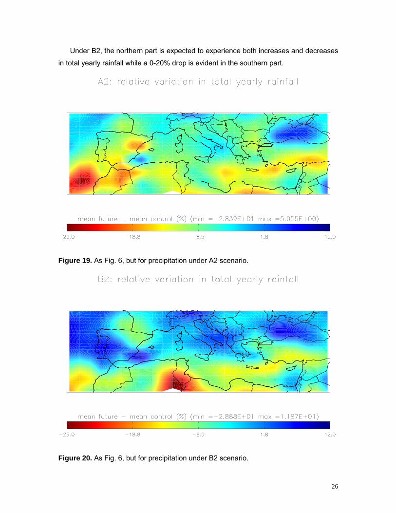
5.4 Precipitation5.4.1 Annual rainfall changes

Figs. 19 & 20 give the variations in the mean total yearly rainfall for both scenarios.

Under scenario A2, a drop in precipitation seems to be the dominant feature of the future

precipitation regime. Under B2, some rainfall increases are expected in the northern part

of the region. Compared to temperature, precipitation exhibits larger differences between

the two scenarios .

Under A2, we can roughly identify two main areas:

� 0-10% drop in precipitation relative to the 1961-1990 values in the northern part

� 10-20% drop in precipitation relative to the reference period values in the southern

part including Spain.

26

Under B2, the northern part is expected to experience both increases and decreases

in total yearly rainfall while a 0-20% drop is evident in the southern part.

Figure 19. As Fig. 6, but for precipitation under A2 scenario.

Figure 20. As Fig. 6, but for precipitation under B2 scenario.

27

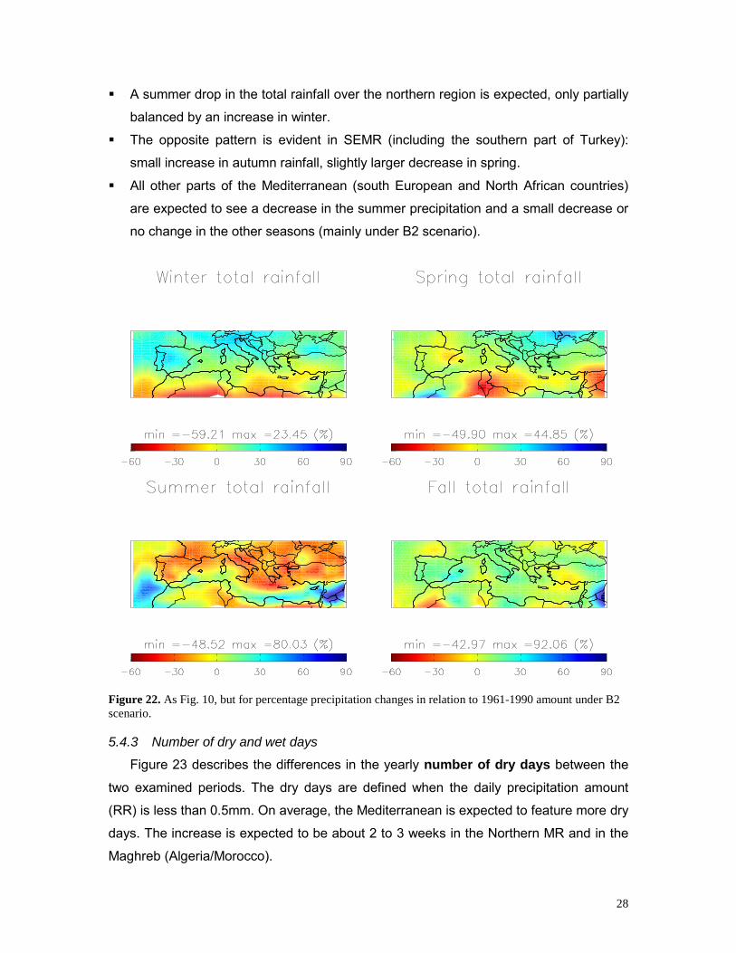
5.4.2 Seasonal rainfall changes

Figs. 21 and 22 represent the relative changes in precipitation between the two

periods and for scenarios A2 and B2 respectively. From these two figures it becomes

evident that:

� Spring and summer rainfall regime exhibits no differences between the two

scenarios.

� Fall seems to experience a little bit more rain under B2 scenario.

� Winter exhibits the main differences between the two scenarios, with more rainfall

under B2, especially in France and Spain.

Figure 21. As Fig. 10, but for percentage precipitation changes in relation to 1961-1990

amount under A2 scenario.

The main feature of the seasonal variations in precipitation is the contrast between

the North - South and winter- summer:

28

� A summer drop in the total rainfall over the northern region is expected, only partially

balanced by an increase in winter.

� The opposite pattern is evident in SEMR (including the southern part of Turkey):

small increase in autumn rainfall, slightly larger decrease in spring.

� All other parts of the Mediterranean (south European and North African countries)

are expected to see a decrease in the summer precipitation and a small decrease or

no change in the other seasons (mainly under B2 scenario).

Figure 22. As Fig. 10, but for percentage precipitation changes in relation to 1961-1990 amount under B2scenario.

5.4.3 Number of dry and wet days

Figure 23 describes the differences in the yearly number of dry days between the

two examined periods. The dry days are defined when the daily precipitation amount

(RR) is less than 0.5mm. On average, the Mediterranean is expected to feature more dry

days. The increase is expected to be about 2 to 3 weeks in the Northern MR and in the

Maghreb (Algeria/Morocco).

29

The increase is likely to be lower along the coast (~2 weeks), but higher inland (3

weeks in the south of France, the Balkans, Turkey, and Italy, and almost a month in the

Iberian peninsula and in Bulgaria).

This increase is balanced by the situation in the greater SEMR (Libya-Egypt-Israel-

Lebanon-Cyprus) where no significant change or even a slight decrease will be

experienced (between -4 and +5 dry days).

Figure 23: Difference between the average yearly number of dry days in the future and in the control years.

RR <0.5 mm defines dry days. Future scenario is A2.

Note that under the B2 scenario, fewer dry days are expected everywhere, which is

not a significant difference between the two scenarios. The results are also very similar if

RR <1mm is used to define dry days (not shown here).

To summarise, we have an increase in general in the number of dry days, ranging

from ~1 month more dry days within the Iberian peninsula to just few extra dry days in

the SEMR or even a slight decrease in Cyprus.

The number of wet days was also examined. One may ask if a dry day increase is

associated with a decrease in the very or extremely wet days or simply in the wet days.

The number of very wet days (RR > 10 mm) does not change much (+/- <3 days on

average, not shown). No change is also seen in the number of extremely wet days(RR > 20 mm, not shown).

Finally, variation of rainy days that fall in the 1-10 mm range is shown in Fig. 24. This

corresponds to the middle range of precipitation. It is expected to drop by 2 weeks in the

North Med, and by a less than a week in the southern Mediterranean (except in the

30

Maghreb where the drop will be closer to 2 weeks). This decrease in the middle range is

associated with the increase in dry days, as clearly seen by comparing Figs. 24 and 23,

and taking into account that no change in the number of very wet days is expected.

Figure 24: Variation in the number of days with precipitation between 1 and 10 mm.

5.4.4 Precipitation intensity

Figure 25 shows the annual maximum amount of total rainfall over 3 days. It is worth

noting that some areas in the North Mediterranean are likely to see this parameter

increasing while their total annual precipitation actually decreases and the number of wet

days remains unchanged. This can imply that when it rains it will rain more intensely and

strongly. This is particularly true in Italy, Western Greece, South of France, and the

northwestern part of the Iberian Peninsula. On the contrary, rainfall is likely to become

less intense over the Southern Mediterranean.

5.4.5 Spells

Changes in the length of wet spells and dry spells (also referred to as droughts) are

examined. Our results show little change in the length of wet (RR> 0.5 or 1mm) or

extremely wet (RR> 10 or 20mm) spells (not shown). This is in accordance with our

results under Section 4.4.3 which show little change in the number of days associated

with these ranges of precipitation.

Greater variations are seen in dry spells. Longer dry spells are likely to be common.

The biggest changes for RR<1mm, shown in Figure 26, are likely to be 2 to 4 weeks

31

increase in the south of Italy and the Peloponese region in Greece, from the south of

Iberian Peninsula to Morocco, and in Libya.

Figure 25. Difference in the annual maximum 3-day cumulative rainfall.

Figure 26. Difference in the length of the longest dry spell (RR<1mm defines dry spells, scenario A2).

Other areas in the SEMR and the Cartagena-Algiers axis do not feature longer dry

spells. On the other hand, the northern part of Algeria, which is expected to have more

dry days, is not expected have longer dry spells. The extra dry days are scattered in

time.

The start and the end of these longest dry spells are also of interest since these are

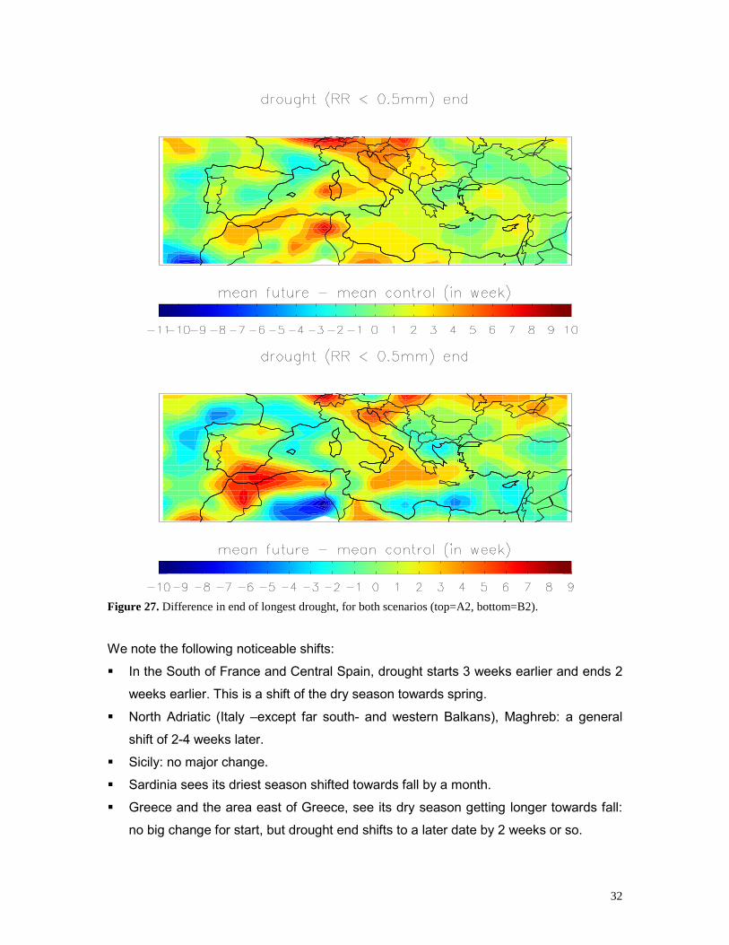
expected to affect agriculture. Fig. 27 (Fig. 28) shows the shift in the end (start) of the

drought.

32

Figure 27. Difference in end of longest drought, for both scenarios (top=A2, bottom=B2).

We note the following noticeable shifts:

� In the South of France and Central Spain, drought starts 3 weeks earlier and ends 2

weeks earlier. This is a shift of the dry season towards spring.

� North Adriatic (Italy –except far south- and western Balkans), Maghreb: a general

shift of 2-4 weeks later.

� Sicily: no major change.

� Sardinia sees its driest season shifted towards fall by a month.

� Greece and the area east of Greece, see its dry season getting longer towards fall:

no big change for start, but drought end shifts to a later date by 2 weeks or so.

33

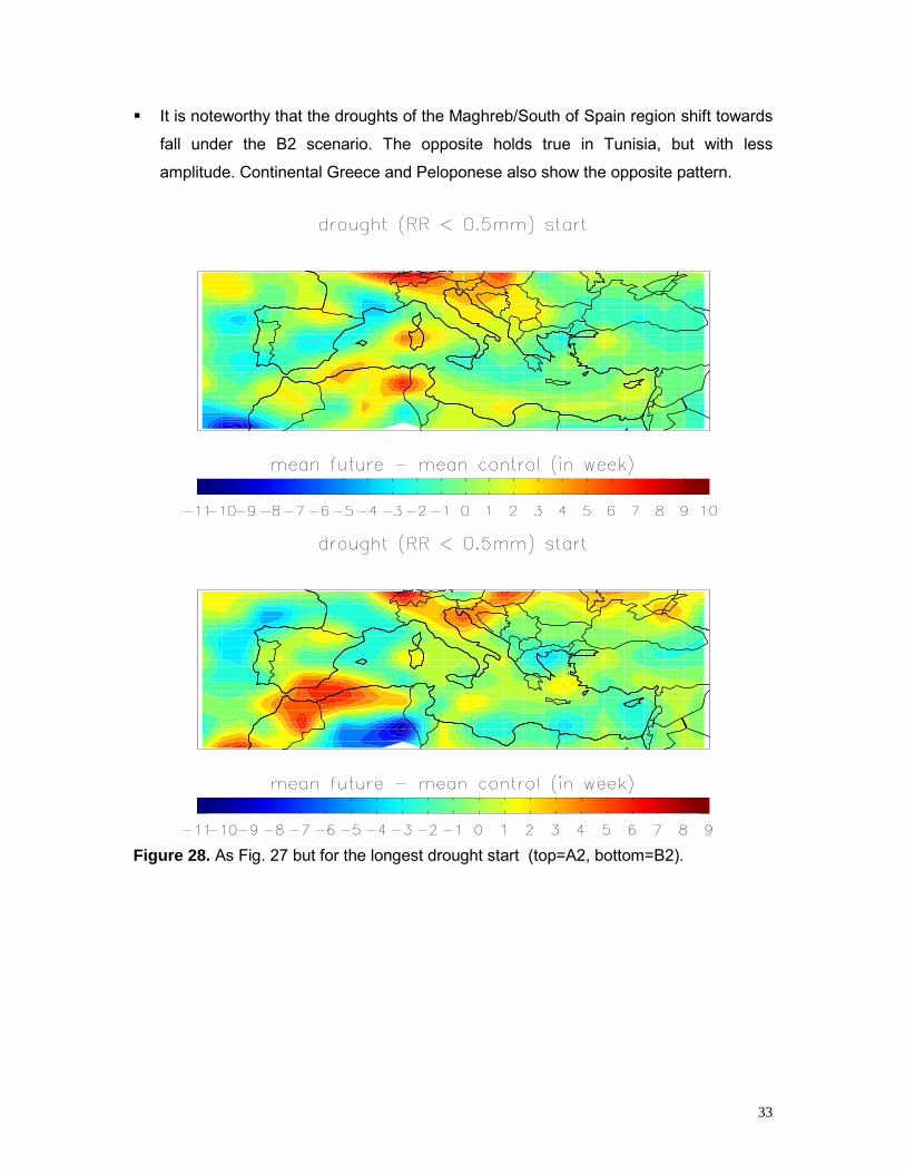
� It is noteworthy that the droughts of the Maghreb/South of Spain region shift towards

fall under the B2 scenario. The opposite holds true in Tunisia, but with less

amplitude. Continental Greece and Peloponese also show the opposite pattern.

Figure 28. As Fig. 27 but for the longest drought start (top=A2, bottom=B2).

35

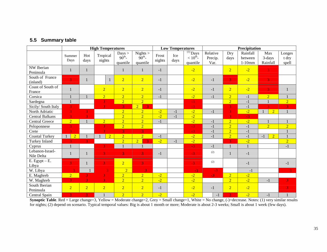
5.5 Summary tableHigh Temperatures Low Temperatures Precipitation

SummerDays

Hotdays

Tropicalnights

Days >90th-

quantile

Nights >90th-

quantile

Frostnights

Icedays

(1) Days< 10th-

quantile

RelativePrecip.

Var.

Drydays

Rainfallbetween1-10mm

Max3-days

Rainfall

Longest dryspell

NW IberianPeninsula 1 1 1 1 -1 -2 2 -2 3

South of France(inland) 3 1 1 2 2 -1 -2 -1 3 -2 3

Coast of South ofFrance 1 2 2 2 -1 -2 -1 2 -2 3 1

Corsica 1 1 2 2 2 -1 -2 -1 2 -1 2 1Sardegna 1 3 2 2 -3 2 -1 1 2Sicily/ South Italy 3 3 3 2 3 -3 3 -1 3 3North Adriatic 3 3 2 2 -2 -1 -2 -1 3 -2 1 2 1Central Balkans 3 3 2 2 -2 -1 -2 3 -3Central Greece 2 1 2 2 2 -1 -2 -1 2 -2 1 1Peloponnese 3 3 2 2 -3 -1 2 -1 2 2Crete 3 3 3 3 -3 -1 2 -1 1Coastal Turkey 1 2 1 1 2 2 2 -1 -2 -1 2 -1 -1 2 1Turkey Inland 3 3 2 2 3 -2 -1 -2 3 -2 2Cyprus 1 3 1 1 -3 -1 1 1 -1Lebanon-Israel-Nile Delta 1 1 3 3 3 -1 -3 (2) 1 -1

E. Egypt – E.Libya 3 1 3 2 3 -3 (2) -1 -1

W. Libya 3 1 3 2 3 -3 -3 -1 3E. Maghreb 2 3 3 2 2 -2 -2 -3 2 -2W. Maghreb 3 3 3 2 2 -2 -2 2 -2 -1 3South IberianPeninsula 2 2 2 2 2 -1 -2 -1 2 -2 3

Central Spain 3 3 1 2 2 -2 -2 -1 3 -2 -1 1Synoptic Table. Red = Large change=3, Yellow = Moderate change=2, Grey = Small change=1, White = No change, (-)=decrease. Notes: (1) very similar resultsfor nights; (2) depend on scenario. Typical temporal values: Big is about 1 month or more; Moderate is about 2-3 weeks; Small is about 1 week (few days).

36

6. Impact analysis6.1 Energy demand

Energy demand is linked to climatic conditions (Giannakopoulos and Psiloglou,

2005) and the relationship of energy demand and temperature is non-linear. The

variability of ambient air temperature is closely linked to energy consumption, whose

maximum values correlate with the extreme values of air temperature (maximum or

minimum). In the Mediterranean region, during January, the maximum values of

energy consumption are related to the appearance of the lowest temperatures.

During the transient season of March-April, energy consumption levels are nearly

constant until about May, while air temperatures are constantly rising. From about

mid-May onwards, and throughout the summer period, any increase in air

temperature translates to an increase in energy consumption mainly due to the

extensive use of air conditioning. The exception is August since most people in the

Mediterranean region tend to take their summer holidays. Another transient period

exists in the months of September and October where energy demand and

consumption are at constant levels. This transient period is followed by a period of

continually increasing energy demand with a peak before the Christmas festive

period. Therefore, it is expected that with warmer weather decreased demand should

be typical in winter and increased demand should be typical in the summer

(Giannakopoulos and Psiloglou, 2005, Valor et al., 2001). Moreover, the effect of

higher temperatures chiefly in the summer is likely to be considerably greater on

peak energy demand than on net demand, suggesting that there will be a need to

install additional generating capacity over and above that needed to cater for

underlying economic growth unless adaptation or mitigation strategies are put into

place.

Since the energy-temperature relationship is non-linear and has distinct winter

and summer branches, it would be more convenient to separate these two branches.

The easiest way to achieve this is to use the idea of Degree-Day, which is defined as

the difference of mean daily temperature from a base temperature.

Base temperature should be the temperature where energy consumption is at its

minimum. If this temperature is chosen, then the degree-day index is positive in the

summer branch and negative in the winter branch. Instead of having both positive

and negative values for this index, the definition of two indices is used: heating

(HDD) and cooling degree days (CDD).

For the calculation of the HDD and CDD indices, the following equations were

used:

37

HDD = max (T* - T, 0) (Eq. 1)

CDD = max (T - T**, 0) (Eq. 2)

where T* and T** are the base temperatures for HDD and CDD respectively, which

can be either the same or different and T is the mean daily temperature as this is

calculated from the daily data of HadCM3 for both the reference and the future

periods.

HDD (CDD) is a measure of the severity of winter (summer) conditions in terms of

the outdoor bry-bulb air temperature, an indication of the sensible heating (cooling)

requirements for the particular location. Kadioğlu et al. (2001) used different base

levels of 15oC and 24oC for the calculations of HDD and CDD in Turkey, respectively.

In our study we use 15oC for the calculation of HDDs and 25oC for the calculation of

CDDs. We identify the changes in energy demand levels by showing differences in

the cumulative numbers of CDDs and HDDs between the reference (1961-1990) and

the future period (2031-2060).

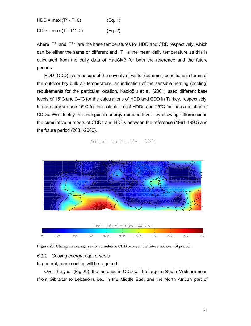
Figure 29. Change in average yearly cumulative CDD between the future and control period.

6.1.1 Cooling energy requirements

In general, more cooling will be required.

Over the year (Fig.29), the increase in CDD will be large in South Mediterranean

(from Gibraltar to Lebanon), i.e., in the Middle East and the North African part of

38

Mediterranean Region. In northern side, the main increase will be in the South

Iberian Peninsula, North-Italy-Balkans-Greece, and South Turkey.

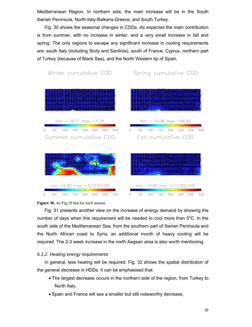
Fig. 30 shows the seasonal changes in CDDs. As expected the main contribution

is from summer, with no increase in winter, and a very small increase in fall and

spring. The only regions to escape any significant increase in cooling requirements

are: south Italy (including Sicily and Sardinia), south of France, Cyprus, northern part

of Turkey (because of Black Sea), and the North Western tip of Spain.

Figure 30. As Fig.29 but for each season.

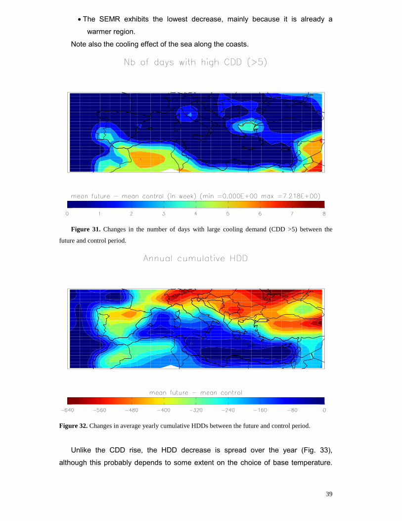
Fig. 31 presents another view on the increase of energy demand by showing the

number of days when this requirement will be needed to cool more than 5oC. In the

south side of the Mediterranean Sea, from the southern part of Iberian Peninsula and

the North African coast to Syria, an additional month of heavy cooling will be

required. The 2-3 week increase in the north Aegean area is also worth mentioning.

6.1.2. Heating energy requirements

In general, less heating will be required. Fig. 32 shows the spatial distribution of

the general decrease in HDDs. It can be emphasised that:

• The largest decrease occurs in the northern side of the region, from Turkey to

North Italy.

• Spain and France will see a smaller but still noteworthy decrease,

39

• The SEMR exhibits the lowest decrease, mainly because it is already a

warmer region.

Note also the cooling effect of the sea along the coasts.

Figure 31. Changes in the number of days with large cooling demand (CDD >5) between the

future and control period.

Figure 32. Changes in average yearly cumulative HDDs between the future and control period.

Unlike the CDD rise, the HDD decrease is spread over the year (Fig. 33),

although this probably depends to some extent on the choice of base temperature.

40

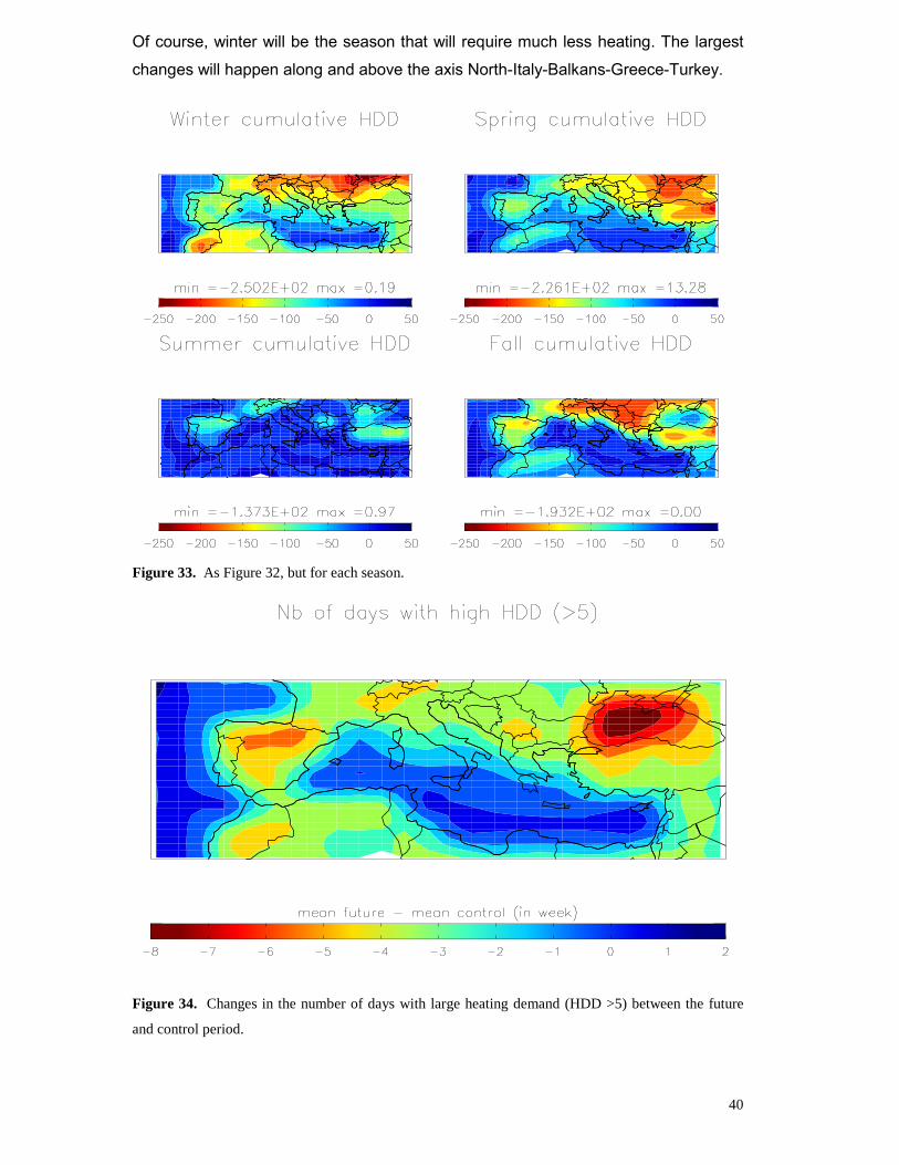
Of course, winter will be the season that will require much less heating. The largest

changes will happen along and above the axis North-Italy-Balkans-Greece-Turkey.

Figure 33. As Figure 32, but for each season.

Figure 34. Changes in the number of days with large heating demand (HDD >5) between the future

and control period.

41

As shown in Fig.34, the decrease in the number of days that require warming more

than 5oC (HDD>5) varies from about 2 weeks along the coast to a month inland.

6.1.3 Summary of impacts on energy demand and supply

Summarising about the CDDs and the HDDs, three areas can be identified:

� South Side of the Mediterranean (North Africa to Syria): very large rise in CDD,

small drop in HDD

� North Side of the Mediterranean (Italy-to-Turkey): small rise in CDD, very large

drop in HDD

� Atlantic Side (Spain / France): small rise in CDD, large drop in HDD

As expected, the northern Mediterranean region is likely to reduce energy use in

the winter due to reduced heating needs. However, during summer, substantial

increases in energy demand are expected everywhere and especially in the south.

The peak in energy demand hence falls in the dry season, which is expected to

become even drier in the future (Section 5.4). A low water supply reduces energy

production from hydroelectric plants, as well as from conventional power plants,

which require water for cooling and for driving the turbines. As a result, energy

demands may not be able to be met in the warm period of the year. Additional

capacity may need to be installed unless adaptation or mitigation strategies are to put

into place. On the other hand, conditions for renewable energy production, such as

solar power, may improve under climate change.

Data in Spain show that the response of mean daily demand for electricity to an

increase of 1°C has steadily increased over the past 30 years (Rodriguez et al.,

2005). The energy demand for per degree of cooling is likely to continue to rise as a

society becomes richer and increased incomes allow the population to afford more

comfort. More air conditioning facilities could be installed. In turn, the heat generated

by air conditioning units could raise temperatures further and further increase the

demand for cooling.

6.2 Forest fire risk6.2.1 About the Fire Weather Index (FWI)

One of the many possible detrimental impacts of anthropogenic climate change is

increased wildfire occurrence. Mediterranean Europe, in particular, has been

identified as likely to suffer hotter, drier summers towards the end of the century

(IPCC, 2001a), and hence potentially increased fire risk (e.g. Pinol et al., 1998,

42

Moriondo et al., 2005). The contribution of meteorological factors to fire risk is

simulated by various non-dimensional indices of fire risk. Viegas et al. (1999)

validated a number of such indices in the Mediterranean against observed fire

occurrence, with the Canadian Fire Weather Index (FWI, van Wagner, 1987)

amongst the best performers. Viegas et al. (2001) demonstrated that in summer, the

slow response of live fine fuel moisture content to meteorological conditions is well

described by the Drought Code sub-component of the FWI system. FWI is also one

of the most widely used indices of fire risk. Hence, it is natural to use output from

climate model simulations (here of HadCM3) of the coming decades (here 2031-

2060) as input to the FWI model to suggest how Mediterranean fire risk may change.

The Canadian Fire Weather Index system is described in detail in van Wagner

(1987). Briefly, it consists of six components that account for the effects of fuel

moisture and wind on fire behaviour. These include numeric ratings of the moisture

content of litter and other fine fuels, the average moisture content of loosely

compacted organic layers of moderate depth, and the average moisture content of

deep, compact organic layers. The remaining components are fire behaviour indices,

which represent the rate of fire spread, the fuel available for combustion, and the

frontal fire intensity; their values rise as the fire danger increases.

Fire risk is low for FWI<15, and increases more rapidly with FWI>15 (Good et al.,

2005). A threshold of FWI>30 was selected as a measure of increased fire risk.

6.2.2 FWI results

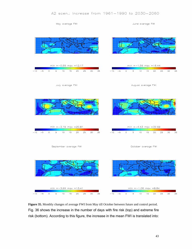
Fig. 35 shows the monthly changes of average FWI from May till October

between the future and the control period. We note that:

• The increase is higher during the summer, with maximum increase in August in

the North Mediterranean inland.

• Balkans, Maghreb, North Adriatic, Central Spain, and Turkey are the most

affected regions.

• South of France is as strongly affected as Spain, but only in August and

September.

• The SEMR (from Lebanon to Libya) sees no increase or decrease.

• The same seems to hold for the islands of Crete, Sardinia, Sicily (southernmost

Italy too), Peloponnese, and Cyprus. Cyprus may even see a small decrease

every month.

• The results are very similar under scenario B2 (not shown).

43

Figure 35. Monthly changes of average FWI from May till October between future and control period.

Fig. 36 shows the increase in the number of days with fire risk (top) and extreme fire

risk (bottom). According to this figure, the increase in the mean FWI is translated into:

44

• 2 to 6 additional weeks of fire risk everywhere, except south Italy and Cyprus and

the SEMR.

• The maximum increase is again inland (Spain, Maghreb, Balkans, North Italy,

and Central Turkey), where at least an additional month with risk of fire has to be

expected.

• A significant proportion of this increase in fire risk is actually extreme fire risk

(FWI>30).

• South of France, Crete, and the coastal area of the rest of Mediterranean Region:

significant increase in the number of days with fire risk (1-4 weeks), but not in the

number of extreme fire risk.

Figure 36. Changes in the number of days with fire risk (top) and extreme fire risk (bottom)between

the future and the control period.

45

To conclude, Fig. 37 shows the number of weeks with fire risk in the future. In the

south part of the Mediterranean, practically the whole year is expected to be a period

of fire risk.

Figure 37. No of weeks with fire risk (FWI>15) in the future period (2031-2060).

6.3 Impacts on tourismAs some measure of the economic importance of summer tourism to the

Mediterranean, 147 million international tourists visited the Mediterranean in 2003

(this is 22% of the international tourism market) and generated US$113 billion for the

region. 70% of these tourists visited just two countries, Italy and Spain. It is very

difficult to model the potential response of tourists to climate change. However, by

discussions with experts at the MICE regional workshop entitled “Impacts of climate

extreme events on Mediterranean tourism and beach holidays”, (which took place in

June 2004 in Crete), it was possible to identify some of the impacts climate change

may have on the tourism industry (Table 1).

Rising temperatures over the Mediterranean region in 2031-2060 will certainly

affect the thermal comfort of tourists and their ability to acclimatise to a region prone

to high temperatures and heatwaves. Rainfall is also projected to decrease, leading

in turn to shortages in the public water supply and more widespread desertification,

which may affect the aesthetics of the region. Water shortages due to extended

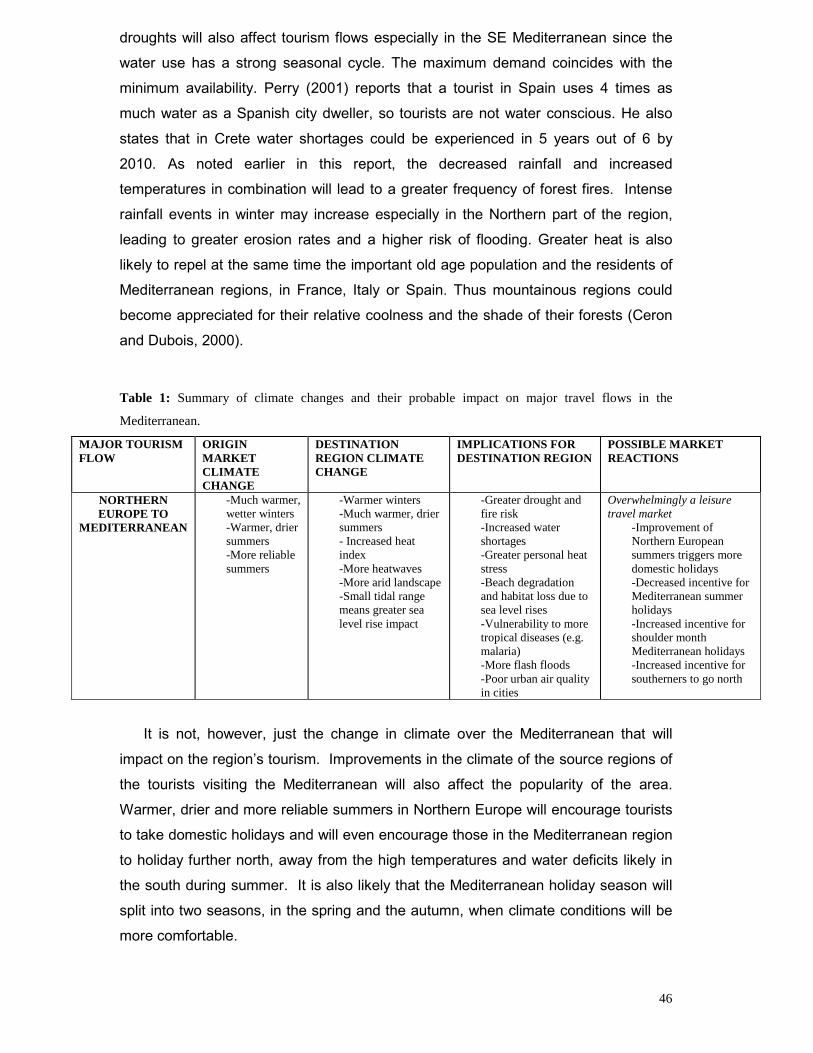
46

droughts will also affect tourism flows especially in the SE Mediterranean since the

water use has a strong seasonal cycle. The maximum demand coincides with the

minimum availability. Perry (2001) reports that a tourist in Spain uses 4 times as

much water as a Spanish city dweller, so tourists are not water conscious. He also

states that in Crete water shortages could be experienced in 5 years out of 6 by

2010. As noted earlier in this report, the decreased rainfall and increased

temperatures in combination will lead to a greater frequency of forest fires. Intense

rainfall events in winter may increase especially in the Northern part of the region,

leading to greater erosion rates and a higher risk of flooding. Greater heat is also

likely to repel at the same time the important old age population and the residents of

Mediterranean regions, in France, Italy or Spain. Thus mountainous regions could

become appreciated for their relative coolness and the shade of their forests (Ceron

and Dubois, 2000).

Table 1: Summary of climate changes and their probable impact on major travel flows in the

Mediterranean.

MAJOR TOURISMFLOW

ORIGINMARKETCLIMATECHANGE

DESTINATIONREGION CLIMATECHANGE

IMPLICATIONS FORDESTINATION REGION

POSSIBLE MARKETREACTIONS

NORTHERNEUROPE TO

MEDITERRANEAN

-Much warmer,wetter winters-Warmer, driersummers-More reliablesummers

-Warmer winters-Much warmer, driersummers- Increased heatindex-More heatwaves-More arid landscape-Small tidal rangemeans greater sealevel rise impact

-Greater drought andfire risk-Increased watershortages-Greater personal heatstress-Beach degradationand habitat loss due tosea level rises-Vulnerability to moretropical diseases (e.g.malaria)-More flash floods-Poor urban air qualityin cities

Overwhelmingly a leisuretravel market

-Improvement ofNorthern Europeansummers triggers moredomestic holidays-Decreased incentive forMediterranean summerholidays-Increased incentive forshoulder monthMediterranean holidays-Increased incentive forsoutherners to go north

It is not, however, just the change in climate over the Mediterranean that will

impact on the region’s tourism. Improvements in the climate of the source regions of

the tourists visiting the Mediterranean will also affect the popularity of the area.

Warmer, drier and more reliable summers in Northern Europe will encourage tourists

to take domestic holidays and will even encourage those in the Mediterranean region

to holiday further north, away from the high temperatures and water deficits likely in

the south during summer. It is also likely that the Mediterranean holiday season will

split into two seasons, in the spring and the autumn, when climate conditions will be

more comfortable.

47

In conclusion:

� Warmer northern European summers encourage an increase in domestic

holidays.

� In a warmer future, there is an increased likelihood of people from the

Mediterranean holidaying in the north.

� More frequent and more intense heat waves and drought are likely to

discourage Mediterranean summer holidays.

� There is likely to be a shift in the Mediterranean holiday season to spring and

autumn.

6.4 Impacts on water resourcesOne of the greatest potential impacts of climate change on human society is

through its effect on water resources. The Mediterranean is already a region,

experiencing moderate to high water stresses and climate change has the potential

to exacerbate further these stresses.

The implications of climate change for water resources stress in the

Mediterranean were assessed by the UK Meteorological Office (Arnell, 1999). First,

river runoff was simulated with a macro-scale hydrological model. Then changes in

national water resource availability were computed (taking into account imports from

upstream), and the estimated volume of water available for use was compared with

the amount withdrawn by water users. For the period in question in this report (2031-

2060), it was projected that runoff decreases substantially in the Mediterranean

Europe, North Africa and the Middle East. The North Mediterranean will see a

50mm/year reduction in runoff while the South (already dry) will experience a

25mm/year decrease or less. However, these changes can be very large in

percentage terms.

The rise in temperature is expected to also affect the timing of streamflow through

the year with particularly large changes in the North Mediterranean, where the higher

winter temperatures mean that a much smaller proportion of winter precipitation falls

as snow to be stored on the land surface until the spring melt. In these areas winter

flows might increase but it is highly likely that spring flows will decrease.

One measure of national water resource stress is the ratio of water used to water

available (although this hides within-country variations and the risk of stress during

drought conditions), and countries using more than 20% of their total annual water

supply are generally held to be exposed to water stress. Using this measure, all

countries around the Mediterranean are expected see an increase in water stress.

48

The sole exception can be Egypt where river runoff from the Nile may actually

increase due to floods in the Central African Nile springs.

Some countries have conducted further studies to illuminate the impact of such

changes on their countries. In the northern Mediterranean, the Spanish Government

estimates that a 1°C increase in the mean annual temperature is likely to lead to a

reduction of 5-14% in water yields in the country. In the extreme case of a 4°C

increase, water yields could reduce by as much as 22% in some regions (Rodriguez

et al., 2005). In the southern Mediterranean, the Algerian Government estimates that

a 1°C rise in mean annual temperature would lead to decreases in precipitation by

15% and in influx of surface waters by 30%. Subsequently, water demand would

exceed available water resources by 800 million m3 (Government of Algeria, 2001).

In the southeastern Mediterranean, the Lebanon Government estimates that by

2050, climate change would be responsible for nearly doubling the water shortage to

350 million m3 of water (Khawli, 1999).

6.5 Impacts on sea level riseResults from the HadCM3 give a projection of a global rise in sea level of 21cm

by the 2050s due to rise in greenhouse gases from human activities (IPCCa, 2001).

This estimate includes direct prediction of thermal expansion combined with

estimates of land-based ice-melt.

However, global mean sea level rise does not manifest itself uniformly around the

world. Regional variations in atmospheric circulation, ocean circulation and warming

rates and the interactions between them have led to significant deviations of

regionally sea level change from the globally averaged trend.

Model projections of regional sea level patterns show very little agreement. For

the Mediterranean, the values range from 1 to 2cm of regional sea level rise per 1 cm

of global sea level rise (IPCCa, 2001). This is due to the low tidal range in the

Mediterranean combined with the limited potential for wetland migration. The most

vulnerable region seems to be the Southern Mediterranean from Turkey to Algeria

where flooding impacts can occur particularly in deltaic countries (such as Egypt).

6.6 Impacts on biodiversityClimate change over the past 30 years has produced numerous shifts in the

distributions and abundances of species. Recent studies have tried to quantify future

changes under different warming scenarios. Thuiller et al. (2005) shows that a 3.6°C

global warming could lead to a loss of over 50% of plant species in the northern

49

Mediterranean and the Mediterranean mountain region, while species loss is likely to

exceed 80% in northcentral Spain and the Cevennes and Massif Central in France.

These results are in the direction of earlier studies (e.g., Thomas et al., 2004)

although estimates of the magnitudes extinction risks are lower than earlier

predictions. Climate change may also have indirect effects on the ecosystem.

Grigulis et al. (2005) shows that increased fires due to climate change could increase

the spread of invasive grass species which in turn, could lead to more frequent and

more intense fires.

ReferencesAbaurrea J, Asín J, Erdozain O, Fernández E, 2001: Climate variability analysis of

temperature series in the Medium Ebro River Basin, In Brunet, M. and López, (Eds.):

Detecting and modelling regional climate change, Springer Verlag, Berlin,

Heidelberg, New York, pp 109-118.

Alpert P, Ben-Gai T, Baharad A, Benjamini Y, Yekutieli D, Colacino M, Diodato L,

Ramis C, Homar V, Romero R, Michaelides S, Manes A, 2002: The paradoxical

increase of Mediterranean extreme daily rainfall in spite of decrease in total values.

Geophys. Res. Lett., 29, art. no.1536.

Bolle, H.-J. (Ed), 2003: Mediterranean Climate – Variability and Trends. Springer

Verlag, Berlin, Heidelberg, New York.

Brunet M, Aguilar E, Saladie O, Sigró J, López D, 1999: Variaciones y tendencias

contemporáneas de la temperatura máxima, mínima y amplitud térmica diaria en el

NE de España. In Raso Nadal, J. M. and Martin-Vide, J. (Eds.): La Climatologia

española en los albores del siglo XXI, Publicaciones de la A.E.C., Serie A, 1,

Barcelona, pp. 103-112.

Brunet M, Aguilar E, Saladie O, Sigró J, López D, 2001a: The variations and trends

of the surface air temperature in the Northeastern of Spain from middle nineteenth

century onwards, In Brunet, M. and López, (Eds.): Detecting and modelling regional

climate change, Springer Verlag, Berlin, Heidelberg, New York, pp 81-93.

Brunet M, Aguilar E, Saladie O, Sigró J, López D, 2001b: A differential response of

Northeastern Spain to asymmetric trends in diurnal warming detected on a global

scale, In Brunet, M. and López, (Eds.): Detecting and modelling regional climate

change, Springer Verlag, Berlin, Heidelberg, New York, pp 95-107.

50

Brunet M, Aguilar E, Saladie O, Sigró J, López D, 2001c: The Spanish Diurnal

Warming: A different pattern to the observed on a global scale, Geophysical

Research Abstracts, 3, 5332.

Brunet M, Aguilar E, Saladie O, Sigró J, López D, 2002: Warming phases in long-

term Spanish temperature change, In 13th Symposium on Global change and

Climate Variations, Orlando 13-17 January 2002, American Meteorological Society,

Boston, pp. 30-32.

Brunetti M, Colacino M, Maugeri M, Nanni T, 2001a: Trends in the daily intensity of

precipitation in Italy from 1951-1996. Int. J. Climatol., 21, 299-316.

Brunetti M, Maugeri M, Nanni T, 2001b: Changes in total precipitation, rainy days and

extreme events in north-eastern Italy. Int. J. Climatol., 21, 861-871.

Ceron, J-P. and G. Dubois, 2000: Tourisme et changement climatique, In Impacts

potentiels du changement climatique en France au XXIème siècle. Premier ministre.

Ministère de l’aménagement du territoire et de l’environnement 1998. pp 104-111.

(deuxième édition 2000).

De Luís M, Raventós J, González-Hidalgo JC, Sánchez JR, Cortina J, 2000: Spatial

analysis of rainfall trends: a case study in Valencia Region (E Spain). Int. J. Climatol.,

20, 1451-1469.

Folland CK, et al., 2001: Observed climate variability and change, in Chapter 2 of

climate change 2001; the scientific basis, Contribution of Working Group I to the

Third Assessment Report of the Intergovernmental Panel on Climate Change, edited

by edited by Houghton JT et al, 881pp., Cambridge University Press, Cambridge, UK

and New York, NY, USA, 2001.

Frei C, Schär C, 2001: Detection probability of trends in rare events: theory and

application to heavy precipitation in the Alpine Region. J. Climate, 14, 1568-1584.

Galán E, Cañada R, Fernández F, Cervera B, 2001: Annual temperature evolution in

the Southern Plateau of Spain from the construction of regional climatic time series,

In Brunet, M. and López, (Eds.): Detecting and modelling regional climate change,

Springer Verlag, Berlin, Heidelberg, New York, pp 119-131

Giannakopoulos C. and J.P. Palutikof, 2004: Modeling climate extreme events: The

EU project MICE for the case study area of Greece The EGGS (11), 30-35.

Giannakopoulos, C. and B.E. Psiloglou, 2005: Trends in energy load demand for

Athens, Greece: Weather and non-weather related factors, submitted to Climate

Research.

Giorgi F, 2002: Variability and trends of sub-continental scale surface climate in the

twentieth century. Part I: Observations, Clim. Dyn., DOI 10.1007/s00382-001-0204-x.

51

Good, P., M.Moriondo, C.Giannakopoulos, M.Bindi, 2005: The meteorological

conditions associated with extreme fire risk in Italy and Greece: relevance to climate

model studies, submitted to Climate Research.

Goodess CM, Jones PD, 2002: Links between circulation and changes in the

characteristics of Iberian rainfall. Int. J. Climatol., 22, 1593-1615.

Government of Algeria, 2001: Elaboration de la stratégie et du plan d’action national

des changements climatiques. 2001. République Algérienne Démocratique et

Populaire, Ministère de l’Aménagement du Territoire et de l’Environnement, Direction

Générale de l’Environnement.Gordon, C., C. Cooper, C.A. Senior, H. Banks, J.M.

Gregory, T.C. Johns, J.F.B. Mitchell and R.A. Wood, 2000: The simulation of SST,

sea ice extents and ocean heat transports in a version of the Hadley Centre coupled

model without flux adjustments. Climate Dynamics, 16, 147-168.

Grigulis, K., Lavorel, S., Davies, I.D., Dossantos, A., Lloret, F. and Vilà M. ,

Landscape-scale positive feedbacks between fire and expansion of the large tussock

grass, Ampelodesmos mauritanica in Catalan shrublands, Global Change Biology

(2005) 11, 1–12.

Hansen J, Ruedy R, Sato M, Imhoff M, Lawrence W, Easterling D, Peterson T, Karl

T, 2001: A closer look at United States and global surface temperature change. J.

Geophys. Res., 106, 23947-23963.

Hewitt C. and D. Griggs, 2004: Ensembles-based predictions of climate changes and

their impacts. Eos, 85, 566.Horcas R, Rasilla D, Fernández-García F, 2001:

Temperature variations and trends in the Segura River Basin. An exploratory

analysis, In Brunet, M. and López, (Eds.): Detecting and modelling regional climate

change, Springer Verlag, Berlin, Heidelberg, New York, pp 133-142.

IPCC, 2001a: Climate Change 2001: The Scientific Basis. Contribution of WG1 to the

Third Assessment Report of the Ingergovernmental Panel on Climate Change.

Cambridge University Press.

IPCC, 2001b: Climate Change 2001: Impacts, Adaptation and Vulnerability.

Contribution of WG2 to the Third Assessment Report of the Ingergovernmental Panel

on Climate Change. Cambridge University Press.

Jacobeit J, Wanner H, Luterbacher J, Beck C, Philipp. A, Sturm K, 2003:

Atmospheric circulation variability in the North-Atlantic-European area since the mid-

seventeenth century. Clim. Dyn. 20, 341-352.

Kadioğlu M, Şen Z, Gültekin L, 2001: Variations and trends in turkish seasonal

heating and cooling degree-days. Climatic Change 49: 209-223.

52

Khawli, 1999: Water Resources: Assessment of Lebanon’s Vulnerability to Climate

Change. Lebanon’s National Communication on Climate Change. Ministry of

Environment, UNDP, GEF. Beirut.

Mariotti A, Struglia MV, 2002: The hydrological cycle in the Mediterranean region and

implications for the water budget of the Mediterranean Sea, J. Climate, 15, 1674-

1690.

Met Office, 1998: Climate change and its impacts, Report: A first look at results from

the Hadley Centre’s new climate model.

Moriondo M., P. Good, R. Durao, M. Bindi, C. Giannakopoulos and J. Corte Real,

2005: Potential impacts of climate change on forest fire risk in the Mediterranean

area, submitted to Climate Research.

Nakicenovic N, Alcamo J, Davis G, de Vries B, Fenhann J, Gaffin S, Gregory K,

Grübler A, Jung TY, Kram T, La Rovere EL, Michaelis L, Mori S, Morita T, Pepper W,

Pitcher H, Price L, Raihi K, Roehrl A, Rogner HH, Sankovski A, Schlesinger M,

Shukla P, Smith S, Swart R, van Rooijen S, Victor N and Dadid Z. 2000. Emissions

scenarios. A Special Report of Working Group III of the Intergovernmental Panel on

Climate Change. Cambridge University Press.

New M, 2005: Arctic climate change with a 2°C global warming. In Rosentrater L

(Ed.): Evidence and Implications of Dangerous Climate Change in the Arctic, WWF

International Arctic Programme..New MG, Hulme M, Jones PD, 2000: Representing

twentieth-century space time climate fields. Part II: development of a 1901-1996

mean monthly terrestrial climatology, J. Climate, 13, 2217-2238.

New M, Todd M, Hulme M, Jones PD, 2001: Precipitation measurements and trends

in the twentieth century, Int. J. Climatol., 21, 1899-1922.

Palutikof J.P, 2004: Understanding the impacts of climate extremes in Europe:

Progress in the MICE project, Geophysical Research Abstracts, Vol. 6, 06200.

Perry, A., 2001: More heat and drought - Can Mediterranean tourism survive and

prosper?, In Proceedings of the First International Workshop on Climate, Tourism

and Recreation, A. Matzarakis and C.R. De Freitas, eds., 1-6, International Society of

Biometeorology.

Pinol, J., Terradas, J. and Lloret, F., 1998: Climate warming, wildfire hazard, and

wildfire occurrence in coastal eastern Spain Climatic Change, 38, 345–357.

Rodriguez and 48 others, 2005: A preliminary assessment of the impacts in Spain

due to the effects of climate change, Ministry of the Environment, Government of

Spain.

53

Pope, V. D., M. L. Gallani, P. R. Rowntree and R. A. Stratton, 2000: The impact of

new physical parametrizations in the Hadley Centre climate model -- HadAM3.

Climate Dynamics, 16: 123-146.

Ramos MC, 2001: Rainfall distribution patterns and their change over time in a

Mediterranean area. Theor. Appl. Climatol., 69, 163-170.

Romero R, Guijarro JA, Alonso S, 1998: A 30-year (1964-1993) daily rainfall data

base for the Spanish Mediterranean regions: First exploratory study. Int. J. Climatol.,

18, 541-560.

Romero R, Ramis C, Guijarro JA, 1999: Daily rainfall patterns in the Spanish

Mediterranean area: an objective classification. Int. J. Climatol., 19, 95-112.

Thomas C.D. and 18 others. 2004. Extinction risks from climate change. Nature, 427,

145–148.

Thuiller W., Lavorel S., Araújo M.B., Sykes M.T. and Prentice I.C. 2005. Climate

change threats to plant diversity in Europe. PNAS 102 (23), 8245–8250.

Türkes M, 1996: Spatial and temporal analysis of annual rainfall variations in Turkey,

Int. J. Climatol., 16, 1057-1076.

Türkes M, 1998: Influence of geopotential heights, cyclone frequency and southern

oscillation on rainfall variations in Turkey, Int. J. Climatol., 18, 649-680.

Valor E., Meneu V. and Caselles V., 2001: Daily air temperature and electricity load

in Spain. J. Appl. Meteor., 40(8), 1413-1421.

van Wagner, C.E., 1987: Development and structure of the canadian forest fire

weather index system. Canadian Forestry Service, Forestry Technical Report35.

Viegas, D.X., Bovio G. Ferreira A. Nosenzo A. and B. Sol, 1999: Comparative Study

of Various Methods of Fire Danger Evaluation in Southern Europe. Int. J. Wildland

Fire, 9, 235–246.

Viegas, D.X., Pinol J. Viegas M.T. and R. Ogaya, 2001: Estimating live fine fuels

moisture content using meteorologically-based indices. Int. J. Wildland Fire, 10, 223–

240.

Xoplaki E, 2002: Climate Variability over the Mediterranean, Ph.D. Thesis, University

of Bern, 193pp. Available at: http://sinus.unibe.ch/klimet/docs/phd_xoplaki.pdf.

Xoplaki E, González-Rouco JF, Luterbacher J, Wanner H, 2003: Mediterranean

summer air temperature variability and its connection to the large-scale atmospheric

circulation and SSTs, Clim. Dyn., 20: 723-739, DOI 10.1007/s00382-003-0304-x.

Impact of a 2° C global temperature rise on the Mediterranean region: Agriculture analysis assessment.

M. Bindi & M. Moriondo Department of Agronomy and Land Management, Florence, Italy

d changes in ime-slice

3 and C4 severe in the

ing is likely to

locations in ange and its associated increase in

CO2 may have little or small positive impacts on yields, provided that additional water demands can be met. The adoption of specific crop management options (e.g. changes in sowing dates or cultivars) may help in reducing the negative responses of agricultural crops to climate change. However, such options could require up to 40% more water for irrigation, which may or may not be available in the future.

Summary The climate change impact analysis on agriculture showed that the expectetemperature and precipitation for SRES-IPCC scenarios A2 and B2 in the t2031-2060 determined a general reduction in yield of agricultural crops (e.g. Csummer crops, legumes, cereals, tuber crops). Reductions in yields are moresouthern Mediterranean than in the northern Mediterranean, even when the fertilizeffect of increased CO2 is taken into account. The southern Mediterranean experience an overall reduction of crop yields due to climate change. In somethe northern Mediterranean, the effects of climate ch

54

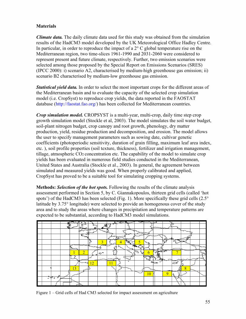
Materia

1 2

3 4 5

6 7

1

ls

imulation Hadley Centre.

rise on the ered to

narios were (SRES)

greenhouse gas emission; ii)

different areas of p simulation

model (i.e. CropSyst) to reproduce crop yields, the data reported in the FAOSTAT tries.

ep crop e soil water budget,

el allows etic

leaf area index, n management,

to simulate crop

ent between d,

alysis hirteen grid cells (called ‘hot

spots’) of the HadCM3 has been selected (Fig. 1). More specifically these grid cells (2.5° latitude by 3.75° longitude) were selected to provide an homogenous cover of the study area and to study the areas where changes in precipitation and temperature patterns are expected to be substantial, accordin odel simulations.

Figure 1 – Grid cells

Climate data. The daily climate data used for this study was obtained from the sresults of the HadCM3 model developed by the UK Meteorological Office In particular, in order to reproduce the impact of a 2° C global temperatureMediterranean region, two time-slices 1961-1990 and 2031-2060 were considrepresent present and future climate, respectively. Further, two emission sceselected among those proposed by the Special Report on Emissions Scenarios (IPCC 2000): i) scenario A2, characterised by medium-high scenario B2 characterised by medium-low greenhouse gas emission. Statistical yield data. In order to select the most important crops for the the Mediterranean basin and to evaluate the capacity of the selected cro

database (http://faostat.fao.org/) has been collected for Mediterranean coun Crop simulation model. CROPSYST is a multi-year, multi-crop, daily time stgrowth simulation model (Stockle et al, 2003). The model simulates thsoil-plant nitrogen budget, crop canopy and root growth, phenology, dry matter production, yield, residue production and decomposition, and erosion. The modthe user to specify management parameters such as sowing date, cultivar gencoefficients (photoperiodic sensitivity, duration of grain filling, maximumetc. ), soil profile properties (soil texture, thickness), fertilizer and irrigatiotillage, atmospheric CO2 concentration etc. The capability of the modelyields has been evaluated in numerous field studies conducted in the Mediterranean, United States and Australia (Stockle et al., 2003). In general, the agreemsimulated and measured yields was good. When properly calibrated and applieCropSyst has proved to be a suitable tool for simulating cropping systems. Methods: Selection of the hot spots. Following the results of the climate anassessment performed in Section 5, by C. Giannakopoulos, t

g to HadCM3 m

2

of Had CM3 selected

for i mpact asse ssme

90

nt on agriculture

8

55

1

11

1 3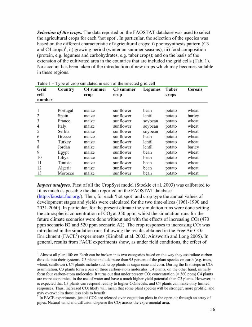

Selection of the crops. The data reported on the FAOSTAT database was usthe agricultural crops for each ‘hot spot’. In particular, the selection of the spbased on the different characteristic of agricultural crops: i) photosynthesisand C4 crops)1, ii) growing period (winter an summer seasons), iii) food(protein, e.g. legumes and carbohydrates, e.g. tuber crops); and on the basis oextension of the cultivated area in the countries that are included the grid cellsNo account ha

ed to select ecies was

pattern (C3 composition

f the (Tab. 1).

s been taken of the introduction of new crops which may becomes suitable

ble 1 – Type of cr ulated i of the selected grid

cell numbe

Country C4 summer crop

C3 summer crop

Legumes Tuber Cereals

in these regions. TaGrid

op sim n each cell

r crops

m sun er an potato m sun er ntil potato m sun er ybean potato m sun er ybean potato m sun er ybean potato m sun er an potato

7 Turk m sun er ntil potato 8 Jord m sun er ntil potato 9 Egypt m sun er an potato

1 Portugal aize flow be wheat 2 Spain aize flow le barley 3 France aize flow so wheat 4 Italy aize flow so wheat 5 Serbia aize flow so wheat 6 Greece aize flow be wheat

ey aize flow le wheat an aize flow le barley aize flow be wheat

10 Libya maize sunflower bean potato wheat

potato wheat wheat

11 Tunisia maize sunflower bean potato wheat 12 Algeria maize sunflower bean 13 Morocco maize sunflower bean potato Impact analyses. First of all the CropSyst model (Stockle et al. 2003) was cafit as much as possible the data

librated to

lues of 1990 and

one setting s for the

future climate scenarios were done without and with the effects of increasing CO2 (470 CO2 was r CO2

005). In ffect of

reported on the FAOSTAT database (http://faostat.fao.org/). Then, for each ‘hot spot’ and crop type the annual vadevelopment stages and yields were calculated for the two time-slices (1961-2031-2060). In particular, for the present climate the simulation runs were dthe atmospheric concentration of CO2 at 350 ppm; whilst the simulation run

ppm scenario B2 and 520 ppm scenario A2). The crop responses to increasingintroduced in the simulation runs following the results obtained in the Free AiEnrichment (FACE2) experiments (Kimball et al. 2002; Ainsworth and Long 2general, results from FACE experiments show, as under field conditions, the e 1 Almost all plant life on Earth can be broken into two categories based on the way they assimdioxide into their systems. C3 plants

ilate carbon include more than 95 percent of the plant species on earth (e.g. trees,

t steps in CO2

plants, on the other hand, initially form four carbon-atom molecules. It turns out that under present CO2 concentration (≈ 360 ppm) C4 plants are more economical in the use of water and have a much higher yield potential than C3 plants. However, it is expected that C3 plants can respond readily to higher CO2 levels, and C4 plants can make only limited responses. Thus, increased CO2 likely will mean that some plant species will be stronger, more prolific, and may overwhelm those less able to benefit. 2 In FACE experiments, jets of CO2 are released over vegetation plots in the open-air through an array of pipes. Natural wind and diffusion disperse the CO2 across the experimental area.

wheat, sunflower). C4 plants include such crop plants as sugar cane and corn. During the firsassimilation, C3 plants form a pair of three carbon-atom molecules. C4

56

CO2 on crop yields is significantly lower than that obtained in controlled environmental studies.

strategies (e.g. f climate r crops (i.e.

t the rest rainfed crops”. Moreover, all the crops were considered

fully fertilised (i.e. no nitrogen stress).

t climate ported in

mer crop, the different

ica which is expected to have lower water availability. Whilst for the irrigated crops (C4 summer

re less

apacity of ach

error is the ses and can

ths study. put with

for individual grid cells while the statistical data from FAO has been collected at the nation level. The climate

on over a gical trend,

pest and disease stresses, etc.) that cannot be reproduced by the model.

e 2. M Absolute r (MAE, % een observ nd simulated crop yields for the Medi nean regi N-W = Por l, Spain, France and Italy, N-E = Serbia, Greece and ey, S ordan, E nd Libya, sia, Algeria and Morocco

Mean olute Error

Finally, the CropSyst model was rerun introducing adaptation managementchanges in sowing dates, cultivar, etc.) that may reduce the negative impact ochange or enhance positive impacts. In all the simulation runs the C4 summemaize) and tuber crops (i.e. potato) were considered as “irrigated crops”, whilsof the crops were considered as “

Results: Crop yields under present climate The simulated crop yields for the presenobtained by calibrating CropSyst model on the basis of the FAO data were reFig. 2. The results showed a pattern of crop yields in rainfed crops (C3 sumlegumes, cereals) that is strongly correlated to the precipitation regimes ofgrid cells. Hence, lower crop yields were seen in regions of Northern Afr

crops and tuber crops) the differences in crop yields among the grid cells weevident and these were mainly driven by the temperature regimes. In order to provide a quantitative estimate of the uncertainties related to the cCropSyst to simulate crop yields, Mean Absolute Errors (MAEs) were calculated for ecrop type in four main regions in the Mediterranean (Table 2). Mean absoluteaverage of the difference between modeled and observed value in all test cabe considered as the average prediction error for CropSyst simulations forMAEs also include inherent errors that arise from the comparison of model outobserved data. Simulated values from CropSyst are calculated

conditions of the grid cells cannot completely represent the average conditination, and the statistical data also include sources of variability (e.g. technolo

Tabl ean Erro ) betw ed amain terra ons: tugaTurk -E = J gypt a S-W = Tuni

Abs (MAE, %) Region C4 summer Legumes C3 summer Tuber crops Cereals

.8 N-W 9.3 4.6 10.8 8.7 9N-E 4.4 1.4 2.1 6.7 S-E 12.1 13.8 4.4 11.7 S-W 13.4 0.9 2.7 3.3

4.3 1.3 6.4

Table 2 shows that CropSyst results match quite closely with the statistical data collected by FAO, with MAEs ranging from less than 1% to under 14%. The MAEs can also be used as a measure of the uncertainties of crop yield estimates due to the bias between observed and simulated yields. The total uncertainty is likely to be larger due to the uncertainties cascaded from the emission scenarios and the global climate model (see Section 4.4 for a discussion of uncertainty cascades).

57

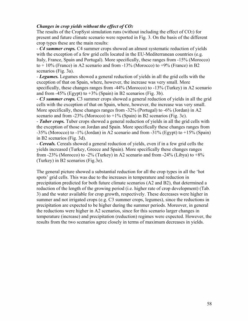
Changes in crop yields without the effect of CO2

The results of the CropSyst simulation runs (without including the effect of Cpresent and future climate scenar

O2) for io were reported in Fig. 3. On the basis of the different

ion of yields es (e.g.

5% (Morocco) e) in B2

ith the as very small. More

2 scenario

s in all the grid se was very small.

in A2

rops showed a general reduction of yields in all the grid cells with s ranges from +15% (Spain)

eneral reduction of yields, even if in a few grid cells the yields increased (Turkey, Greece and Spain). More specifically these changes ranges

a) to +8%

l the ‘hot

ermined a lopment) (Tab.

higher in reductions in

precipitation are expected to be higher during the summer periods. Moreover, in general the reductions were higher in A2 scenarios, since for this scenario larger changes in temperature (increase) and precipitation (reduction) regimes were expected. However, the results from the two scenarios agree closely in terms of maximum decreases in yields.

crop types these are the main results: - C4 summer crops. C4 summer crops showed an almost systematic reductwith the exception of a few grid cells located in the EU-Mediterranean countriItaly, France, Spain and Portugal). More specifically, these ranges from -1to + 10% (France) in A2 scenario and from -13% (Morocco) to +9% (Francscenarios (Fig. 3a). - Legumes. Legumes showed a general reduction of yields in all the grid cells wexception of that on Spain, where, however, the increase wspecifically, these changes ranges from -44% (Morocco) to -13% (Turkey) in Aand from -45% (Egypt) to +3% (Spain) in B2 scenarios (Fig. 3b). - C3 summer crops. C3 summer crops showed a general reduction of yieldcells with the exception of that on Spain, where, however, the increaMore specifically, these changes ranges from -32% (Portugal) to -6% (Jordan)scenario and from -23% (Morocco) to +1% (Spain) in B2 scenarios (Fig. 3c). - Tuber crops. Tuber cthe exception of those on Jordan and Spain. More specifically these change-35% (Morocco) to -1% (Jordan) in A2 scenario and from -31% (Egypt) toin B2 scenarios (Fig. 3d). - Cereals. Cereals showed a g

from -23% (Morocco) to -2% (Turkey) in A2 scenario and from -24% (Liby(Turkey) in B2 scenarios (Fig.3e). The general picture showed a substantial reduction for all the crop types in alspots’ grid cells. This was due to the increases in temperature and reduction inprecipitation predicted for both future climate scenarios (A2 and B2), that detreduction of the length of the growing period (i.e. higher rate of crop deve3) and the water available for crop growth, respectively. These decreases were summer and not irrigated crops (e.g. C3 summer crops, legumes), since the

58

0 2 4 6

Portugal

Spain

France

Italy

Serbia

Greece

Turkey

Jordan

Egypt

Libya

Tunisia

Algeria

Morocco

8b

0 2 4 6

Portugal

Spain

France

Italy

Serbia

Greece

Turkey

Jordan

Egypt

Libya

Tunisia

Algeria

Morocco

a8

c0 2 4 6

Portugal

Spain

France

Italy

Serbia

Greece

Turkey

Jordan

Egypt

Libya

Tunisia

Algeria

Morocco

8d

0 2 4 6

Portugal

Spain

France

Italy

Serbia

Greece

Turkey

Jordan

Egypt

Libya

Tunisia

Algeria

Morocco

8

e0 2 4 6

Portugal

Spain

Serbia

Greece

Turkey

Jordan

Egypt

Libya

Tunisia

Algeria

Morocco

France

Italy

8

Figure 2- Crop yields (t ha-1) in the selected ‘hot spots’ grid cells: a) C4 summer crop, b) legumes, c) C3 summer crop, d) tuber crops, e) cereals.

59

-55 -45 -35 -25 -15 -5 5 15

Portugal

Spain

France

Italy

Serbia

Greece

Turkey

Jordan

Egypt

Libya

Tunisia

Algeria

Morocco

B2A2

b-55 -45 -35 -25 -15 -5 5 15

Portugal

Spain

France

Italy

Serbia

Greece

Turkey

Jordan

Egypt

Libya

Tunisia

Algeria

Morocco

B2A2

a

-55 -45 -35 -25 -15 -5 5 15

Portugal

Spain

France

Italy

Serbia

Greece

Turkey

Jordan

Egypt

Libya

Tunisia

Algeria

Morocco

B2A2

d-55 -45 -35 -25 -15 -5 5 15

Portugal

Spain

France

Italy

Serbia

Greece

Turkey

Jordan

Egypt

Libya

Tunisia

Algeria

Morocco

B2A2

c

e-55 -45 -35 -25 -15 -5 5 15

Serbia

Greece

Turkey

Jordan

Egypt

Libya

Tunisia

Algeria

Morocco

Figure 3- Impact of climate change on crop yields without CO2 effect: a) C4 summer crop, b) legumes, c) C3 summer crop, d) tuber crops, e) cereals. The changes reported in the figures were expressed as % and obtained as differences between the mean yields of the two futures and the present yields.

Portugal

Spain

France

Italy B2A2

60

Table 3 – Mean length of the growing season for the different crop types under the present cenario and me hange ce

Crop type Length (days) A2 (% change) B2 (% change) climate s an percentage c d under future s narios

C4 summer crop 126.3 -8.0 -7.5

mer crop 131.2 -6.7 -6.4 108.0 -5.9 -5.7

crops 170.4 -5.5 -4.7 -1.7 -1.8

C3 sumLeguTuber

mes

Cereals 214.0

Syst simulation runs (including the effect of CO2) for present and ops types

lds in the grid , Tunisia,

increase. ce) in A2

a general reduction of yields in all the grid cells with the

anges ranges ) to +15%

the grid ls located on Northern and South-western shores of the Mediterranean basin; whereas

antially al) to +6% B2 scenarios (Fig.

r crops showed an inconsistent response among selected grid cells, nd

cenario and from -27% (Egypt) to +30% (Jordan) in

e changes m -19% (Libya) to

n tropical lizing effect an, er climate,

but is not able to completely offset the losses. In the cooler northeastern Mediterranean, CO2 increase and the associated climate change result in little net effect on most crops, provided that the increase in water demands, especially for irrigated crops, can be satisfied (Table 4). Similarly in the northwestern Mediterranean, yields of irrigated crop may increase if water demands can be met. However, rainfed summer crops are likely to experience a net reduction in yield, even when the fertilizing effect of CO2 is considered.

Changes in crop yields with the effect of CO2 The results of the Cropfuture climate scenario were reported in Fig. 4. On the basis of the different crthese are the main results: - C4 summer crops. C4 summer crops showed a prevalent reduction in yiecells located in the African and Asian Mediterranean countries (e.g. MoroccoJordan, etc.); whereas on the European grid cells yields showed a consistentMore specifically, these changes ranges from -12% (Morocco) to + 16% (Franscenario and from -11% (Egypt) to +13% (France) in B2 scenarios (Fig. 4a). - Legumes. Legumes showedexception of those on Spain, Turkey and Greece. More specifically, these chfrom -39% (Morocco) to +2% (Turkey) in A2 scenario and from -41% (Egypt(Spain) in B2 scenarios (Fig. 4b). - C3 summer crops. C3 summer crops showed a general reduction of yields in celin the grid cells located on the Southern or Eastern shores, yields were substunchanged. More specifically, these changes ranges from -21% (Portug(Turkey) in A2 scenario and from -16% (Morocco) to +11% (Spain) in4c). - Tuber crops. Tubewith a general reduction of yields in those on the African shores of the basin, aprevalent increase in the rest. More specifically these changes ranges from -25%(Morocco) to +16% (Jordan) in A2 sB2 scenarios (Fig. 4d). - Cereals. Cereals showed a prevalent increase in yields. More specifically thesranges from -15% (Morocco) to +13% (Tunisia) in A2 scenario and fro+19% (Turkey) in B2 scenarios (Fig. 4e). The general picture showed that the effect of climate change on agriculture iareas are likely to be more severe than in temperate areas, even when the fertiof increased CO2 is considered (Table 4). In the warmer southern Mediterraneincreases in CO2 help to reduce the loss in yield arising from a warmer and dri

61

-40 -30 -20 -10 0 10 20 30

Portugal

Spain

France

Italy

Serbia

Greece

Turkey

Jordan

Egypt

Libya

Tunisia

Algeria

Morocco

B2A2

b-40 -30 -20 -10 0 10 20 30

Portugal

Spain

France

Italy

Serbia

Greece

Turkey

Jordan

Egypt

Libya

Tunisia

Algeria

Morocco

B2A2

a

c-40 -30 -20 -10 0 10 20 30

Portugal

Spain

France

Italy

Serbia

Greece

Turkey

Jordan

Egypt

Libya

Tunisia

Algeria

Morocco

B2A2

d-40 -30 -20 -10 0 10 20 30

Portugal

Spain

France

Italy

Serbia

Greece

Turkey

Jordan

Egypt

Libya

Tunisia

Algeria

Morocco

B2A2

e

-40 -30 -20 -10 0 10 20 30

Portugal

Serbia

Greece

Turkey

Jordan

Egypt

Libya

Tunisia

Algeria

Morocco

Figure 4- Impact of climate change on crop yields with CO2 effect: a) C4 summer crop, b) legumes, c) C3 summer crop, d) tuber crops, e) cereals. The changes reported in the figures were expressed as % and obtained as differences between the mean yields of the two futures and the present yields.

Spain

France

Italy B2A2

62

Table 4 – Percentage changes of crop yields for the main Mediterranean regions: N-WSpain, France and Italy, N

= Portugal, -E = Serbia, Greece and Turkey, S-E = Jordan, Egypt and Libya, S-W =

Tunisia, Al ria a it O W O2

ge nd Morocco W hout C 2 ith C

A2-A -A B2-A C4 summe 0.1 5 4 8.78

B2 A2-A r N-W 9 .80 .19

NS

-4.43 -1

.54

.260.607.89 1. 4 -9 -

S -1 .87 8.94 9.38

-2 .90 - 3.42 4.38N -1 .59 8.11 -7.19

2. -2 S -3 .26 - 5.81 3.92

r N -2 .79 - 0.44 2.41

5. -6 - S -7.44 9 .66

S -1 4 - .81 .33

-1 .37 4.24 4.872. -6 -

SS

-1 2 - .77 4.31 -2 .88 - .10 3.28

-E -2 - 0.21 -E 4 -6.70

-W 2 - - -6.37 Legumes N-W 4 1 -1 -4.86 -E 8 - 0.97 S-E -3 72 -36.43 3.30 -30.15

-W 3 2 -2 -18.48 C3 summe -W 1 1 -1 -2.85 N-E -1 57 .92 5.44 0.96

-E -8.1 3 -0.41 -W 9.9 11 -10 -4.34 Tubers N-W 0 - 7.53 N-E -2 50 .80 9.33 4.39

-E 8.2 15 - -5.66 -W 5 12 -1 -1.55 Cereals N-W -10.97 -3.49 -0.29 4.68

9 3.71 4.39 12.49 S-E -15.08 -17.17 -4.88 -10.15 N-E -6.7

S-W -13.77 -11.29 -3.42 -3.77 Impacts of adaptation options

r present nt crops

ultivars with a d positive effects

– 1% with with longer growing

tandard rage

+4% with an .

early sowing of standard cultivars determined positive effects on crop yields. More specifically, the average changes of yields passed from – 3% with standard cultivar to +5% and -1% with an early sowing and cultivar with longer growing cycles, respectively (Fig. 5c). - Tuber crops. Tuber crops showed that the introduction of cultivars with a shorter growing cycle or the early sowing of standard cultivars determined positive effects on crop yields. More specifically, the average changes of yields passed from – 3% with

The results of the CropSyst simulation runs (including adaptation strategies) foand future climate scenarios were reported in Fig. 5. On the basis of the differetypes these are the main results: - C4 summer crops. C4 summer crops showed that the introduction of clonger growing cycle or the early sowing of standard cultivars determineon crop yields. More specifically, the average changes of yields passed fromstandard cultivar to +1% and +9% with an early sowing and cultivarcycles, respectively (Fig. 5a). - Legumes. Legumes showed that the introduction of an early sowing of scultivars determined positive effects on crop yields. More specifically, the avechanges of yields passed from – 15% with standard cultivar to -10% andearly sowing and cultivar with longer growing cycles, respectively (Fig. 5b)- C3 summer crops. C3 summer crops showed that the introduction of an

63

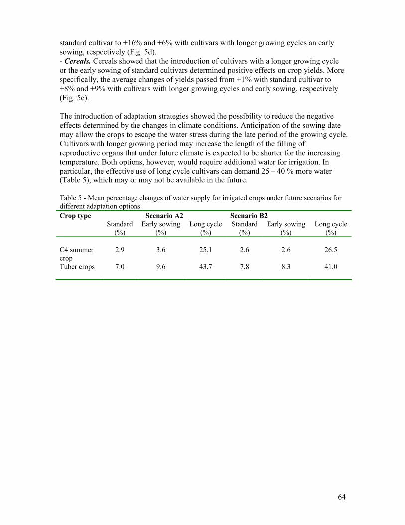
standard cultivar to +16% and +6% with cultivars with longer growing cycles an early

ing cycle p yields. More

ltivar to d +9% with cultivars with longer growing cycles and early sowing, respectively

(Fig. 5e).

gative n of the sowing date

owing cycle. of he increasing

dditional water for irrigation. In particular, the effective use of long cycle cultivars can demand 25 – 40 % more water

Table 5 - M n o p ga e narios for different adaptation optionCrop type cenario A2 Scenario B2

sowing, respectively (Fig. 5d). - Cereals. Cereals showed that the introduction of cultivars with a longer growor the early sowing of standard cultivars determined positive effects on crospecifically, the average changes of yields passed from +1% with standard cu+8% an

The introduction of adaptation strategies showed the possibility to reduce the neeffects determined by the changes in climate conditions. Anticipatiomay allow the crops to escape the water stress during the late period of the grCultivars with longer growing period may increase the length of the fillingreproductive organs that under future climate is expected to be shorter for ttemperature. Both options, however, would require a

(Table 5), which may or may not be available in the future.

ean perce tage changess

f water sup ly for irri ted crops und r future sce

S Standard

(%) ly sowin

(%) ong cy

(%) Standa

(%) Early sowing

(%Long cycle

(%)

Ear g L cle rd )

C4 summer crop

2.9

3.6

25.1

2.6

2.6

26.5

Tuber crops 7.0

9.6

43.7

7.8

8.3

41.0

64

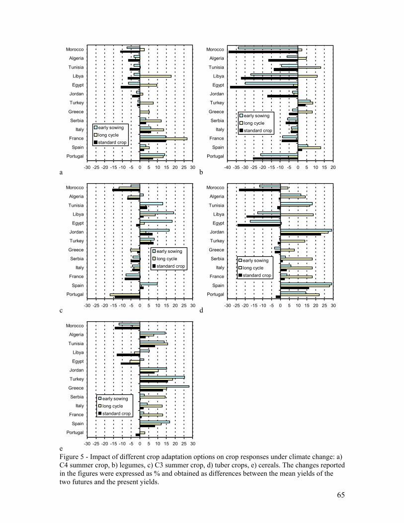
-30 -25 -20 -15 -10 -5 0 5 10 15 20 25 30

Portugal

Spain

France

Italy

Serbia

Greece

Turkey

Jordan

Egypt

Libya

Tunisia

Algeria

Morocco

early sowinglong cyclestandard crop

b-40 -35 -30 -25 -20 -15 -10 -5 0 5 10 15 20

Portugal

Spain

France

Italy

Serbia

Greece

Turkey

Jordan

Egypt

Libya

Tunisia

Algeria

Morocco

early sowinglong cyclestandard crop

a

-30 -25 -20 -15 -10 -5 0 5 10 15 20 25 30

Portugal

Spain

France

Italy

Serbia

Greece

Turkey

Jordan

Egypt

Libya

Tunisia

Algeria

Morocco

early sowinglong cyclestandard crop

d-30 -25 -20 -15 -10 -5 0 5 10 15 20 25 30

Portugal

Spain

France

Italy

Serbia

Greece

Turkey

Jordan

Egypt

Libya

Tunisia

Algeria

Morocco

early sowinglong cyclestandard crop

c

e-30 -25 -20 -15 -10 -5 0 5 10 15 20 25 30

Serbia

Greece

Turkey

Jordan

Egypt

Libya

Tunisia

Algeria

Morocco

early sowing

Figure 5 - Impact of different crop adaptation options on crop responses under climate change: a) C4 summer crop, b) legumes, c) C3 summer crop, d) tuber crops, e) cereals. The changes reported in the figures were expressed as % and obtained as differences between the mean yields of the two futures and the present yields.

Portugal

Spain

France

Italy long cyclestandard crop

65

Discussions and Conclusions

ion reduction of

uction of the ons in

ler northern account.

ields due to editerranean, the effects of climate

change and its associated increase in CO2 may have little or small positive impacts on

ates may be crop yield determined

re up to 40%

heric losses under a of ground d (Morgan et

d by it, zone concentrations are expected to increase globally. Thus, if the effects of to be included in an assessment of crop yields in the Mediterranean under a

n presented in

References -air CO2

tosynthesis, -372

2001) Ecosystems and their goods and services, In: Climate Change 2001: Impacts, Adaptation and Vulnerability, McCarthy, JJ

BA, Kobayashi K, Bindi M (2002) Responses of agricultural crops to free-air CO enrichment. Advances in Agronomy, 77: 293-368

Long SP (2003) How does elevated ozone impact soybean? A meta-analysis of photosynthesis, growth and yield. Plant, Cell and Environment 2003 26:8 1317 Stockle CO, Donatelli M, Nelson R (2003) CropSyst, a cropping systems simulation model. Eur J Agron 18: 289-307

Our study showed that the increases in temperature and reduction in precipitatpredicted for both future climate scenarios (A2 and B2) lead to a substantial yields for all the crop types in all the ‘hot spots’ grid cells, through the redlength of the growing period and the water available for crop growth. Reductiyields are more severe in the warmer southern Mediterranean than in the cooMediterranean, even when the fertilizing effect of increased CO2 is taken intoThe southern Mediterranean is likely to experience an overall reduction of yclimate change. In some locations in the northern M

yields, provided that additional water demands can be met. Strategies such as early sowing dates or cultivar with slower development rconsidered as helpful options to reduce some of the reductions in by the changes in climate conditions. However, such options could requimore water for irrigation, which may or may not be available in the future. Moreover, according to recent studies on the effects on crop yields of troposppollutants such ozone, there is reason to believe that our estimates of yieldfuture scenario may be conservative. Current and increased concentrationslevel ozone have been shown to lead to decreases in plant biomass and yielal., 2003; Gitay et al., 2001). Independently of climate change, but exacerbatesurface oozone are future climate scenario, the results are likely to greater yield reductions thathis report.

Ainsworth EA, Long SP (2005) What have we learned from 15 years of freeenrichment (FACE)? A meta-analytic review of responses to rising CO2 in phocanopy properties and plant production. New Phytol., 165:351 Gitay H, Brown S, Easterling W and Jallow B. (

Canziani, OF, Leary, NA, Dokken DJ and White KS (ed.), p.735-800. Kimball

2

Morgan PB, Ainsworth EA,

66

67