
Climate Change 2001: Synthesis Report - Home | …€¦ · · 2018-04-14Question 3 Question 4...
151
Core Writing Team Daniel L. Albritton, Terry Barker, Igor A. Bashmakov, Osvaldo Canziani, Renate Christ, Ulrich Cubasch, Ogunlade Davidson, Habiba Gitay, David Griggs, John Houghton, Joanna House, Zbigniew Kundzewicz, Murari Lal, Neil Leary, Christopher Magadza, James J. McCarthy, John F.B. Mitchell, Jose Roberto Moreira, Mohan Munasinghe, Ian Noble, Rajendra Pachauri, Barrie Pittock, Michael Prather, Richard G. Richels, John B. Robinson, Jayant Sathaye, Stephen Schneider, Robert Scholes, Thomas Stocker, Narasimhan Sundararaman, Rob Swart, Tomihiro Taniguchi, and D. Zhou All IPCC Authors Editorial Team David J. Dokken, Maria Noguer, Paul van der Linden, Cathy Johnson, Jiahua Pan, and the GRID-Arendal Design Studio Based on a draft prepared by: Climate Change 2001: Synthesis Report Edited by: Robert T. Watson The World Bank and the Core Writing Team
Transcript of Climate Change 2001: Synthesis Report - Home | …€¦ · · 2018-04-14Question 3 Question 4...

Core Writing TeamDaniel L. Albritton, Terry Barker, Igor A. Bashmakov, Osvaldo Canziani, Renate Christ, Ulrich Cubasch, Ogunlade Davidson, Habiba Gitay, David Griggs, John Houghton, Joanna House, Zbigniew Kundzewicz, Murari Lal, Neil Leary, Christopher Magadza, James J. McCarthy, John F.B. Mitchell, Jose Roberto Moreira, Mohan Munasinghe, Ian Noble, Rajendra Pachauri, Barrie Pittock, Michael Prather, Richard G. Richels, John B. Robinson, Jayant Sathaye, Stephen Schneider, Robert Scholes, Thomas Stocker, Narasimhan Sundararaman, Rob Swart, Tomihiro Taniguchi, and D. Zhou
All IPCC Authors
Editorial TeamDavid J. Dokken, Maria Noguer, Paul van der Linden, Cathy Johnson, Jiahua Pan, and the GRID-Arendal Design Studio
Based on a draft prepared by:
Climate Change 2001:Synthesis Report
Edited by:
Robert T. WatsonThe World Bank
and theCore Writing Team

Synthesis ReportQuestion 1Question 2Question 3Question 4Question 5Question 6Question 7Question 8Question 9
AnnexesA. Authors and Expert ReviewersB. Glossary of TermsC. Acronyms, Abbreviations, and Units
Summary for Policymakers
3537 40 47 57 61 68 74 84 91
149A-1B-1C-1
1
Climate Change 2001:Synthesis Report
Contents

An Assessment of the Intergovernmental Panel on Climate Change
This summary, approved in detail at IPCC Plenary XVIII (Wembley, United Kingdom, 24-29 September 2001), represents the formally agreed statement of the IPCC concerning key findings and uncertainties contained in the Working Group contributions to the Third Assessment Report.
Climate Change 2001:Synthesis Report
Robert T. Watson, Daniel L. Albritton, Terry Barker, Igor A. Bashmakov, Osvaldo Canziani, Renate Christ, Ulrich Cubasch, Ogunlade Davidson, Habiba Gitay, David Griggs, John Houghton, Joanna House, Zbigniew Kundzewicz, Murari Lal, Neil Leary, Christopher Magadza, James J. McCarthy, John F.B. Mitchell, Jose Roberto Moreira, Mohan Munasinghe, Ian Noble, Rajendra Pachauri, Barrie Pittock, Michael Prather, Richard G. Richels, John B. Robinson, Jayant Sathaye, Stephen Schneider, Robert Scholes, Thomas Stocker, Narasimhan Sundararaman, Rob Swart, Tomihiro Taniguchi, D. Zhou, and many IPCC authors and reviewers
Summary for Policymakers
Based on a draft prepared by:

2
Climate Change 2001 Synthesis Report
IPCC Third Assessment Report
Introduction
In accordance with a decision taken at its Thirteenth Session (Maldives, 22 and 25-28 September1997) and other subsequent decisions, the IPCC decided:
To include a Synthesis Report as part of its Third Assessment ReportThat the Synthesis Report would provide a policy-relevant, but not policy-prescriptive, synthesisand integration of information contained within the Third Assessment Report and also drawingupon all previously approved and accepted IPCC reports that would address a broad range ofkey policy-relevant, but not policy-prescriptive, questionsThat the questions would be developed in consultation with the Conference of the Parties(COP) to the United Nations Framework Convention on Climate Change (UNFCCC).
The following nine questions were based on submissions by governments and were approved bythe IPCC at its Fifteenth Session (San Jose, Costa Rica, 15-18 April 1999).
Question 1
What can scientific, technical, and socio-economic analyses contribute tothe determination of what constitutes dangerous anthropogenicinterference with the climate system as referred to in Article 2 of theFramework Convention on Climate Change?
Natural, technical, and social sciences can provide essentialinformation and evidence needed for decisions on what constitutes“dangerous anthropogenic interference with the climate system.” Atthe same time, such decisions are value judgments determinedthrough socio-political processes, taking into account considerationssuch as development, equity, and sustainability, as well asuncertainties and risk.
The basis for determining what constitutes “dangerous anthropogenic interference”will vary among regions—depending both on the local nature and consequencesof climate change impacts, and also on the adaptive capacity available to copewith climate change—and depends upon mitigative capacity, since the magnitudeand the rate of change are both important. There is no universally applicable best set ofpolicies; rather, it is important to consider both the robustness of different policy measures againsta range of possible future worlds, and the degree to which such climate-specific policies can beintegrated with broader sustainable development policies.
The Third Assessment Report (TAR) provides an assessment of new scientificinformation and evidence as an input for policymakers in their determination ofwhat constitutes “dangerous anthropogenic interference with the climate system.”It provides, first, new projections of future concentrations of greenhouse gases in theatmosphere, global and regional patterns of changes and rates of change in temperature,precipitation, and sea level, and changes in extreme climate events. It also examines possibilitiesfor abrupt and irreversible changes in ocean circulation and the major ice sheets. Second, it providesan assessment of the biophysical and socio-economic impacts of climate change, with regard torisks to unique and threatened systems, risks associated with extreme weather events, the distributionof impacts, aggregate impacts, and risks of large-scale, high-impact events. Third, it provides anassessment of the potential for achieving a broad range of levels of greenhouse gasconcentrations in the atmosphere through mitigation and information about how adaptation canreduce vulnerability.
••
•
Q1.1
Q1.2
Q1.3-6
Q1

3
Summary for Policymakers
��������������������� ������ ����� �
����������������������������
��������� ������������������������ ���
���������������� �����
������������ ������������������� ����������
������������ � ���� ���������������� ������ ����
!��������������!��������
� ������������"� �����
����� ��� �� ������������� ���
� ���������������# ���������������
"��������$��������
"��������
Figure SPM-1: Climate change – an integrated framework. Schematic and simplified representation of anintegrated assessment framework for considering anthropogenic climate change. The yellow arrows show thecycle of cause and effect among the four quadrants shown in the figure, while the blue arrow indicates thesocietal response to climate change impacts. See the caption for Figure 1-1 for an expanded description ofthis framework.
Q1
Q1 Figure 1-1
Q1.7
Q1.8
An integrated view of climate change considers the dynamics of the complete cycleof interlinked causes and effects across all sectors concerned (see Figure SPM-1).The TAR provides new policy-relevant information and evidence with regard to all quadrants ofFigure SPM-1. A major new contribution of the Special Report on Emissions Scenarios (SRES)was to explore alternative development paths and related greenhouse gas emissions, and the TARassessed preliminary work on the linkage between adaptation, mitigation, and development paths.However, the TAR does not achieve a fully integrated assessment of climate change because ofthe incomplete state of knowledge.
Climate change decision making is essentially a sequential process under generaluncertainty. Decision making has to deal with uncertainties including the risk of non-linear and/or irreversible changes and entails balancing the risks of either insufficient or excessive action,and involves careful consideration of the consequences (both environmental and economic), theirlikelihood, and society’s attitude towards risk.

4
Climate Change 2001 Synthesis Report
IPCC Third Assessment Report
The climate change issue is part of the larger challenge of sustainable development.As a result, climate policies can be more effective when consistently embeddedwithin broader strategies designed to make national and regional developmentpaths more sustainable. This occurs because the impact of climate variability and change,climate policy responses, and associated socio-economic development will affect the ability ofcountries to achieve sustainable development goals. Conversely, the pursuit of those goals will inturn affect the opportunities for, and success of, climate policies. In particular, the socio-economicand technological characteristics of different development paths will strongly affect emissions,the rate and magnitude of climate change, climate change impacts, the capability to adapt, and thecapacity to mitigate.
The TAR assesses available information on the timing, opportunities, costs, benefits,and impacts of various mitigation and adaptation options. It indicates that there areopportunities for countries acting individually, and in cooperation with others, to reduce costs ofmitigation and adaptation and to realize benefits associated with achieving sustainable development.
Question 2
What is the evidence for, causes of, and consequences of changes in theEarth’s climate since the pre-industrial era?
Has the Earth’s climate changed since the pre-industrial era at theregional and/or global scale? If so, what part, if any, of the observedchanges can be attributed to human influence and what part, if any,can be attributed to natural phenomena? What is the basis for thatattribution?What is known about the environmental, social, and economicconsequences of climate changes since the pre-industrial era withan emphasis on the last 50 years?
The Earth’s climate system has demonstrably changed on both globaland regional scales since the pre-industrial era, with some of thesechanges attributable to human activities.
Human activities have increased the atmospheric concentrations of greenhousegases and aerosols since the pre-industrial era. The atmospheric concentrations of keyanthropogenic greenhouse gases (i.e., carbon dioxide (CO
2), methane (CH
4), nitrous oxide (N
2O),
and tropospheric ozone (O3)) reached their highest recorded levels in the 1990s, primarily due to
the combustion of fossil fuels, agriculture, and land-use changes (see Table SPM-1). The radiativeforcing from anthropogenic greenhouse gases is positive with a small uncertainty range; that fromthe direct aerosol effects is negative and smaller; whereas the negative forcing from the indirecteffects of aerosols on clouds might be large but is not well quantified.
An increasing body of observations gives a collective picture of a warming worldand other changes in the climate system (see Table SPM-1).
Globally it is very likely that the 1990s was the warmest decade, and 1998 thewarmest year, in the instrumental record (1861–2000) (see Box SPM-1). The increasein surface temperature over the 20th century for the Northern Hemisphere is likely to have beengreater than that for any other century in the last thousand years (see Table SPM-1). Insufficientdata are available prior to the year 1860 in the Southern Hemisphere to compare the recent warmingwith changes over the last 1,000 years. Temperature changes have not been uniform globally buthave varied over regions and different parts of the lower atmosphere.
Q1.9-10
Q1.11
Q2.2
Q2.4-5
Q2.6
Q2.7
(a)
(b)
Q2

5
Summary for Policymakers Q1 | Q2
Table SPM-1 20th century changes in the Earth’s atmosphere, climate, and biophysical system.a
Indicator
Concentration indicators
Atmospheric concentration of CO2
Terrestrial biospheric CO2 exchange
Atmospheric concentration of CH4
Atmospheric concentration of N2O
Tropospheric concentration of O3
Stratospheric concentration of O3
Atmospheric concentrations of HFCs, PFCs, and SF6
Weather indicators
Global mean surface temperature
Northern Hemisphere surface temperature
Diurnal surface temperature range
Hot days / heat index
Cold / frost days
Continental precipitation
Heavy precipitation events
Frequency and severity of drought
Observed Changes
280 ppm for the period 1000-1750 to 368 ppm in year 2000 (31±4% increase).
Cumulative source of about 30 Gt C between the years 1800 and 2000; but during the 1990s, a net sink of about 14±7 Gt C.
700 ppb for the period 1000-1750 to 1,750 ppb in year 2000 (151±25% increase).
270 ppb for the period 1000-1750 to 316 ppb in year 2000 (17±5% increase).
Increased by 35±15% from the years 1750 to 2000, varies with region.
Decreased over the years 1970 to 2000, varies with altitude and latitude.
Increased globally over the last 50 years.
Increased by 0.6±0.2°C over the 20th century; land areas warmed more than the oceans (very likely).
Increased over the 20th century greater than during any other century in the last 1,000 years; 1990s warmest decade of the millennium (likely).
Decreased over the years 1950 to 2000 over land: nighttime minimum temperatures increased at twice the rate of daytime maximum temperatures (likely).
Increased (likely).
Decreased for nearly all land areas during the 20th century (very likely).
Increased by 5-10% over the 20th century in the Northern Hemisphere (very likely), although decreased in some regions (e.g., north and west Africa and parts of the Mediterranean).
Increased at mid- and high northern latitudes (likely).
Increased summer drying and associated incidence of drought in a few areas (likely). In some regions, such as parts of Asia and Africa, the frequency and intensity of droughts have been observed to increase in recent decades.
Box SPM-1 Confidence and likelihood statements.
Where appropriate, the authors of the Third Assessment Report assigned confidence levels that represent their collective judgment in the validity of a conclusion based on observational evidence, modeling results, and theory that they have examined. The following words have been used throughout the text of the Synthesis Report to the TAR relating to WGI findings: virtually certain (greater than 99% chance that a result is true); very likely (90–99% chance); likely (66–90% chance); medium likelihood (33–66% chance); unlikely (10–33% chance); very unlikely (1–10% chance); and exceptionally unlikely (less than 1% chance). An explicit uncertainty range (±) is a likely range. Estimates of confidence relating to WGII findings are: very high (95% or greater), high (67–95%), medium (33–67%), low (5–33%), and very low (5% or less). No confidence levels were assigned in WGIII.
There is new and stronger evidence that most of the warming observed over thelast 50 years is attributable to human activities. Detection and attribution studiesconsistently find evidence for an anthropogenic signal in the climate record of the last 35 to 50years. These studies include uncertainties in forcing due to anthropogenic sulfate aerosols andnatural factors (volcanoes and solar irradiance), but do not account for the effects of other types ofanthropogenic aerosols and land-use changes. The sulfate and natural forcings are negative overthis period and cannot explain the warming; whereas most of these studies find that, over the last50 years, the estimated rate and magnitude of warming due to increasing greenhouse gases alone
Q2.9-11
Q2 Box 2-1

6
Climate Change 2001 Synthesis Report
IPCC Third Assessment Report
are comparable with, or larger than, the observed warming. The best agreement between modelsimulations and observations over the last 140 years has been found when all the aboveanthropogenic and natural forcing factors are combined, as shown in Figure SPM-2.
Changes in sea level, snow cover, ice extent, and precipitation are consistent witha warming climate near the Earth’s surface. Examples of these include a more activehydrological cycle with more heavy precipitation events and shifts in precipitation, widespreadretreat of non-polar glaciers, increases in sea level and ocean-heat content, and decreases in snowcover and sea-ice extent and thickness (see Table SPM-1). For instance, it is very likely that the20th century warming has contributed significantly to the observed sea-level rise, through thermalexpansion of seawater and widespread loss of land ice. Within present uncertainties, observationsand models are both consistent with a lack of significant acceleration of sea-level rise during the20th century. There are no demonstrated changes in overall Antarctic sea-ice extent from the years1978 to 2000. In addition, there are conflicting analyses and insufficient data to assess changes inintensities of tropical and extra-tropical cyclones and severe local storm activity in the mid-latitudes.Some of the observed changes are regional and some may be due to internal climate variations,natural forcings, or regional human activities rather than attributed solely to global human influence.
Observed changes in regional climate have affected many physicaland biological systems, and there are preliminary indications thatsocial and economic systems have been affected.
Table SPM-1 20th century changes in the Earth’s atmosphere, climate, and biophysical system.a (continued)
Indicator
Biological and physical indicators
Global mean sea level
Duration of ice cover of rivers and lakes
Arctic sea-ice extent and thickness
Non-polar glaciers
Snow cover
Permafrost
El Niño events
Growing season
Plant and animal ranges
Breeding, flowering, and migration
Coral reef bleaching
Economic indicators
Weather-related economic losses
Observed Changes
Increased at an average annual rate of 1 to 2 mm during the 20th century.
Decreased by about 2 weeks over the 20th century in mid- and high latitudes of the Northern Hemisphere (very likely).
Thinned by 40% in recent decades in late summer to early autumn (likely) and decreased in extent by 10-15% since the 1950s in spring and summer.
Widespread retreat during the 20th century.
Decreased in area by 10% since global observations became available from satellites in the 1960s (very likely).
Thawed, warmed, and degraded in parts of the polar, sub-polar, and mountainous regions.
Became more frequent, persistent, and intense during the last 20 to 30 years compared to the previous 100 years.
Lengthened by about 1 to 4 days per decade during the last 40 years in the Northern Hemisphere, especially at higher latitudes.
Shifted poleward and up in elevation for plants, insects, birds, and fish.
Earlier plant flowering, earlier bird arrival, earlier dates of breeding season, and earlier emergence of insects in the Northern Hemisphere.
Increased frequency, especially during El Niño events.
Global inflation-adjusted losses rose an order of magnitude over the last 40 years (see Q2 Figure 2-7). Part of the observed upward trend is linked to socio-economic factors and part is linked to climatic factors.
This table provides examples of key observed changes and is not an exhaustive list. It includes both changes attributable to anthropogenic climate change and those that may be caused by natural variations or anthropogenic climate change. Confidence levels are reported where they are explicitly assessed by the relevant Working Group. An identical table in the Synthesis Report contains cross-references to the WGI and WGII reports.
a
Q2.12-19
Q2.20 & Q2.25

7
Summary for Policymakers
Figure SPM-2: Simulating the Earth’s temperature variations (°C) and comparing the results to themeasured changes can provide insight to the underlying causes of the major changes. A climate modelcan be used to simulate the temperature changes that occur from both natural and anthropogenic causes. Thesimulations represented by the band in (a) were done with only natural forcings: solar variation and volcanicactivity. Those encompassed by the band in (b) were done with anthropogenic forcings: greenhouse gasesand an estimate of sulfate aerosols. And those encompassed by the band in (c) were done with both naturaland anthropogenic forcings included. From (b), it can be seen that the inclusion of anthropogenic forcingsprovides a plausible explanation for a substantial part of the observed temperature changes over the pastcentury, but the best match with observations is obtained in (c) when both natural and anthropogenic factorsare included. These results show that the forcings included are sufficient to explain the observed changes, butdo not exclude the possibility that other forcings may also have contributed.
����� ��� �������������%� ����� ��� �������������%�
&�'�(��� ����� ������� & '�"� ���������� �������
����
����
���
���
���
���� ���� ���� ����
�� ����� ��
�����������
���� ���� ���� ��������
����
���
���
���
�� ����� ��
�����������
����� ���� ������������������ �� ��������������� ��� �� ��������������� �)*+,
����
����
���
���
���
����
����
���
���
���
����� ��� �������������%�
&�'�(��� ���-�"� ���������� ���
����
����
���
���
���
�� ����� ��
���������������
����
���
���
���
���� ���� ���� ����
Recent regional changes in climate, particularly increases in temperature, havealready affected hydrological systems and terrestrial and marine ecosystems inmany parts of the world (see Table SPM-1). The observed changes in these systems1 arecoherent across diverse localities and/or regions and are consistent in direction with the expectedeffects of regional changes in temperature. The probability that the observed changes in the expecteddirection (with no reference to magnitude) could occur by chance alone is negligible.
Q2
Q2 Figure 2-4
Q2.21-24
There are 44 regional studies of over 400 plants and animals, which varied in length from about 20 to 50 years,mainly from North America, Europe, and the southern polar region. There are 16 regional studies covering about100 physical processes over most regions of the world, which varied in length from about 20 to 150 years.
1

8
Climate Change 2001 Synthesis Report
IPCC Third Assessment Report
The rising socio-economic costs related to weather damage and to regional variationsin climate suggest increasing vulnerability to climate change. Preliminary indicationssuggest that some social and economic systems have been affected by recent increases in floodsand droughts, with increases in economic losses for catastrophic weather events. However, becausethese systems are also affected by changes in socio-economic factors such as demographic shiftsand land-use changes, quantifying the relative impact of climate change (either anthropogenic ornatural) and socio-economic factors is difficult.
Question 3
What is known about the regional and global climatic, environmental, andsocio-economic consequences in the next 25, 50, and 100 years associatedwith a range of greenhouse gas emissions arising from scenarios used inthe TAR (projections which involve no climate policy intervention)?
To the extent possible evaluate the:Projected changes in atmospheric concentrations, climate, and sea levelImpacts and economic costs and benefits of changes in climate andatmospheric composition on human health, diversity and productivity ofecological systems, and socio-economic sectors (particularly agricultureand water)The range of options for adaptation, including the costs, benefits, andchallengesDevelopment, sustainability, and equity issues associated with impactsand adaptation at a regional and global level.
Carbon dioxide concentrations, globally averaged surface temperature,and sea level are projected to increase under all IPCC emissions scenariosduring the 21st century.2
For the six illustrative SRES emissions scenarios, the projected concentration ofCO2 in the year 2100 ranges from 540 to 970 ppm, compared to about 280 ppm inthe pre-industrial era and about 368 ppm in the year 2000. The different socio-economicassumptions (demographic, social, economic, and technological) result in the different levels offuture greenhouse gases and aerosols. Further uncertainties, especially regarding the persistenceof the present removal processes (carbon sinks) and the magnitude of the climate feedback on theterrestrial biosphere, cause a variation of about -10 to +30% in the year 2100 concentration, aroundeach scenario. Therefore, the total range is 490 to 1,260 ppm (75 to 350% above the year 1750 (pre-industrial) concentration). Concentrations of the primary non-CO
2 greenhouse gases by year 2100
are projected to vary considerably across the six illustrative SRES scenarios (see Figure SPM-3).
Projections using the SRES emissions scenarios in a range of climate modelsresult in an increase in globally averaged surface temperature of 1.4 to 5.8°C overthe period 1990 to 2100. This is about two to ten times larger than the central valueof observed warming over the 20th century and the projected rate of warming isvery likely to be without precedent during at least the last 10,000 years, based onpaleoclimate data. Temperature increases are projected to be greater than those in the SecondAssessment Report (SAR), which were about 1.0 to 3.5°C based on six IS92 scenarios. The higherprojected temperatures and the wider range are due primarily to lower projected sulfur dioxide(SO
2) emissions in the SRES scenarios relative to the IS92 scenarios. For the periods 1990 to
2025 and 1990 to 2050, the projected increases are 0.4 to 1.1°C and 0.8 to 2.6°C, respectively. By
Projections of changes in climate variability, extreme events, and abrupt/non-linear changes are covered in Question 4.
Q3.2
Q3.3-5
Q3.6-7 & Q3.11
Q3
••
•
•
2
Q2.25-26

9
Summary for Policymakers
the year 2100, the range in the surface temperature response across different climate models forthe same emissions scenario is comparable to the range across different SRES emissions scenariosfor a single climate model. Figure SPM-3 shows that the SRES scenarios with the highest emissionsresult in the largest projected temperature increases. Nearly all land areas will very likely warmmore than these global averages, particularly those at northern high latitudes in winter.
Globally averaged annual precipitation is projected to increase during the 21stcentury, though at regional scales both increases and decreases are projected oftypically 5 to 20%. It is likely that precipitation will increase over high-latitude regions in bothsummer and winter. Increases are also projected over northern mid-latitudes, tropical Africa, andAntarctica in winter, and in southern and eastern Asia in summer. Australia, Central America, andsouthern Africa show consistent decreases in winter rainfall. Larger year-to-year variations inprecipitation are very likely over most areas where an increase in mean precipitation is projected.
Glaciers are projected to continue their widespread retreat during the 21st century.Northern Hemisphere snow cover, permafrost, and sea-ice extent are projected to decrease further.The Antarctic ice sheet is likely to gain mass, while the Greenland ice sheet is likely to lose mass(see Question 4).
Global mean sea level is projected to rise by 0.09 to 0.88 m between the years 1990and 2100, for the full range of SRES scenarios, but with significant regionalvariations. This rise is due primarily to thermal expansion of the oceans and melting of glaciersand ice caps. For the periods 1990 to 2025 and 1990 to 2050, the projected rises are 0.03 to 0.14m and 0.05 to 0.32 m, respectively.
Projected climate change will have beneficial and adverse effects onboth environmental and socio-economic systems, but the larger thechanges and rate of change in climate, the more the adverse effectspredominate.
The severity of the adverse impacts will be larger for greater cumulative emissionsof greenhouse gases and associated changes in climate (medium confidence). Whilebeneficial effects can be identified for some regions and sectors for small amounts of climate change,these are expected to diminish as the magnitude of climate change increases. In contrast manyidentified adverse effects are expected to increase in both extent and severity with the degree ofclimate change. When considered by region, adverse effects are projected to predominate for muchof the world, particularly in the tropics and subtropics.
Overall, climate change is projected to increase threats to human health, particularlyin lower income populations, predominantly within tropical/subtropical countries.Climate change can affect human health directly (e.g., reduced cold stress in temperate countriesbut increased heat stress, loss of life in floods and storms) and indirectly through changes in theranges of disease vectors (e.g., mosquitoes),3 water-borne pathogens, water quality, air quality,and food availability and quality (medium to high confidence). The actual health impacts will bestrongly influenced by local environmental conditions and socio-economic circumstances, and bythe range of social, institutional, technological, and behavioral adaptations taken to reduce the fullrange of threats to health.
Ecological productivity and biodiversity will be altered by climate change and sea-level rise, with an increased risk of extinction of some vulnerable species (high tomedium confidence). Significant disruptions of ecosystems from disturbances such as fire,drought, pest infestation, invasion of species, storms, and coral bleaching events are expected to
Q2 | Q3
Q3.8 & Q3.12
Q3.14
Q3.9 & Q3.13
Q3.16
Q3.15
Q3.17
Q3.18-20
Eight studies have modeled the effects of climate change on these diseases—five on malaria and three on dengue.Seven use a biological or process-based approach, and one uses an empirical, statistical approach.
3

*�+*�,
*�-$
*�+�
+�
$.���
���� ���
��
��
& '��51����������&����'
)��
���
����
&�'��!6����������&����!6'
�)
��
�(
&�'�(15����������&���('
��
���
���
&�'��51����������&����'
&�'��51������ �����&���'
&�'��!6������ �����&�� '
&'�(15������ �����&�� '
&�'����������� �����&����'
'��
���
9��
���
����
'��
���
���
��(
���
(��
���
����
'���&�'
����������������� ��� �������� ����� �����
$� ���� ��
$� � ������
$� ��������
$� ���� ������
")��4�������
7��� �����7�!��� ����������7����!���
"1
414)
'�
,#��*������ ����������������!��� �������������!������&� ��!��������0������������&�#4� �� �00� ������#���0�������������������������� ������#����!���4������#����0��������������!��&����������!!����������#� �������2������ ������#������������������������������4���0��������� ����4���������������� � � �� ���� ��� � � �� � � � ��� � � �� 4 �& � � # ��
���������� ������������������� ���!!����������0�����0�����������,#��*����������!��� ����� 0�������#�������0���#�� ������ ���� ��������������������!����#� ���� ��#��������#�����������������,#���#����*�����0���������������#�������#�������#� ���� ���0#����:!��� �����������;*�-$<4 ����!��� ��������� � ��� �;*�, < 4 � � �� ��� ���� ��� ��� ��
�������;*�+<�;&#������ �����������!��������� ��� � ������#��� � � ������0�� � ��� ��������������4����#�������0�����#������� ����0��������������00 ����� ����������00 ����������������#� ����<�
���� ���� ����
���� ���� ����
���� ���� ����
���� ���� ����
���� ���� ����
���� ���� ����
���� ���� ����
���� ���� ����
�����������������������
�������������������� �����
�����������
���������������
��� ����������
�����������������������
�������������������� �����
�����������������������
�������������������� �����
�����������
���������������
��� ���������������������
���������������
��� ����������
")��8�")�8����")4
10
Climate Change 2001 Synthesis Report
IPCC Third Assessment Report

�����������
�������������
�������!�����������
�������������� �������
"��#��
���������� $�������
�������!����������� %���� &
$ $$ $$$ $% %
�
�
�
'
(
�
)
���
%�
�
�
�
'
(
�
)
���
%�
*�+*�,
*�-$
*�+�
+�
$.���
���� ���
/������������������������0����1��2�����!0�0 �������� ��!!�����
.����������� ���
�
�
(
)
&�'������ ��� �������&%�'
���
���
��(
��)
���
���
&�'����������� ����&�'
&/'�.����������� ����&0��1' &�'��������
���� ���������
�
��
+�����#&��#��������������0��������������� ���� �
+�����#&��#��������������0��������������� ���� �
���� ��������
���� ��������
����� ��� ���������2��������� .�������� �����
* �$.���� ������� �� �.�3.����� 0�
�� ������� �� �.�3.����� 0�
�� ������� �� �.�3.����� 0�
,#��*������ ����������������!��� ������������������#�����������&� ���,#������� �����#��������� !��� ����������0�����������!� �� ������������-���� ����0������������������������ ��� ��� � � �� & �4 �&# � �# ����� � � �� ��������� �������������00� ������3��������� 0��������0������ �������� ���������� � � �0 � � �� � 0 � � � �� � � � � � �� � & � # �� � ����#� ���� ��#���������!�������������� &����#����#������� �����
,#��+������ ����������������!��� �����������������������&� ��&� �#��#�������� �� 00� ������#���0�������������������������� ������#����!���4��������#��*������ ���4����&��#���0����#��������������������������&��������������������!������������4�&��#������ ������ ������ �� ��� ���� � �� ������#������������!�� �����������������!!���������#� ������,#����0#������� ���� �� � � � � � � �� �� � � � � � 4 �� � � � 4 �� � ������������ ����������� ���4���� ��������0�����5����4�����&��#����������� �� ������������������
,#��+������ ����������������!��� �������������&� �����&#��#��#����0#���������� �� � � � � � � �� �� � � � � � 4 �� � � � 4 �� � ������������ ����������� �����$�������&� ��&��#�������� �������������� �� �00� ����4���������� &����#���*�4�������������� ��� ��!����������� 0����4����� ������0���������������������#� ���� ��#������#�������#�+������*������ ������6#� ���#������������� �����������&���������������� �0��������������� ��5����4�� � �!�������� �� ���������� � ��� ��
�����������
�����������������������
����
�����������
���������������
��� ����������
* �.�3.����� 0���� ������ ������������������
�����������5��������#����������������������!����7������� ������������8�����������!���0����*�����������0����������!���!������ �������� ����������������
.�������� �����
�������33
�����������������������
����
���������������
��� ����������
���������������� �����
���������������� �����
�� ������� �� �.�3.����� 0�
"1 4) 41
11
Summary for Policymakers Q3
Figure SPM-3: The different socio-economic assumptions underlying the SRES scenarios result in different levels offuture emissions of greenhouse gases and aerosols. These emissions in turn change the concentration of these gases andaerosols in the atmosphere, leading to changed radiative forcing of the climate system. Radiative forcing due to the SRES scenarios results in projectedincreases in temperature and sea level, which in turn will cause impacts. The SRES scenarios do not include additional climate initiatives and noprobabilities of occurrence are assigned. Because the SRES scenarios had only been available for a very short time prior to production of the TAR,the impacts assessments here use climate model results that tend to be based on equilibrium climate change scenarios (e.g., 2xCO2), a relativelysmall number of experiments using a 1% per year CO
2 increase transient scenario, or the scenarios used in the SAR (i.e., the IS92 series). Impacts
in turn can affect socio-economic development paths through, for example, adaptation and mitigation. The highlighted boxes along the top of thefigure illustrate how the various aspects relate to the integrated assessment framework for considering climate change (see Figure SPM-1).
Q3 Figure 3-1

12
Climate Change 2001 Synthesis Report
IPCC Third Assessment Report
increase. The stresses caused by climate change, when added to other stresses on ecologicalsystems, threaten substantial damage to or complete loss of some unique systems and extinctionof some endangered species. The effect of increasing CO
2 concentrations will increase net primary
productivity of plants, but climate changes, and the changes in disturbance regimes associatedwith them, may lead to either increased or decreased net ecosystem productivity (mediumconfidence). Some global models project that the net uptake of carbon by terrestrial ecosystemswill increase during the first half of the 21st century but then level off or decline.
Models of cereal crops indicate that in some temperate areas potential yields increasewith small increases in temperature but decrease with larger temperature changes(medium to low confidence). In most tropical and subtropical regions, potential yieldsare projected to decrease for most projected increases in temperature (mediumconfidence). Where there is also a large decrease in rainfall in subtropical and tropical dryland/rainfed systems, crop yields would be even more adversely affected. These estimates include someadaptive responses by farmers and the beneficial effects of CO
2 fertilization, but not the impact of
projected increases in pest infestations and changes in climate extremes. The ability of livestockproducers to adapt their herds to the physiological stresses associated with climate change ispoorly known. Warming of a few °C or more is projected to increase food prices globally, and mayincrease the risk of hunger in vulnerable populations.
Climate change will exacerbate water shortages in many water-scarce areas of theworld. Demand for water is generally increasing due to population growth and economicdevelopment, but is falling in some countries because of increased efficiency of use. Climatechange is projected to substantially reduce available water (as reflected by projected runoff) inmany of the water-scarce areas of the world, but to increase it in some other areas (mediumconfidence) (see Figure SPM-4). Freshwater quality generally would be degraded by higher watertemperatures (high confidence), but this may be offset in some regions by increased flows.
The aggregated market sector effects, measured as changes in gross domesticproduct (GDP), are estimated to be negative for many developing countries for allmagnitudes of global mean temperature increases studied (low confidence), andare estimated to be mixed for developed countries for up to a few °C warming (lowconfidence) and negative for warming beyond a few degrees (medium to lowconfidence). The estimates generally exclude the effects of changes in climate variability andextremes, do not account for the effects of different rates of climate change, only partially accountfor impacts on goods and services that are not traded in markets, and treat gains for some ascanceling out losses for others.
Populations that inhabit small islands and/or low-lying coastal areas are at particularrisk of severe social and economic effects from sea-level rise and storm surges.Many human settlements will face increased risk of coastal flooding and erosion, and tens ofmillions of people living in deltas, in low-lying coastal areas, and on small islands will face risk ofdisplacement. Resources critical to island and coastal populations such as beaches, freshwater,fisheries, coral reefs and atolls, and wildlife habitat would also be at risk.
The impacts of climate change will fall disproportionately upon developing countriesand the poor persons within all countries, and thereby exacerbate inequities inhealth status and access to adequate food, clean water, and other resources.Populations in developing countries are generally exposed to relatively high risks of adverse impactsfrom climate change. In addition, poverty and other factors create conditions of low adaptivecapacity in most developing countries.
Adaptation has the potential to reduce adverse effects of climatechange and can often produce immediate ancillary benefits, but willnot prevent all damages.
Q3.22
Q3.21
Q3.25
Q3.23
Q3.33
Q3.26

13
Summary for Policymakers
Numerous possible adaptation options for responding to climate change have beenidentified that can reduce adverse and enhance beneficial impacts of climate change,but will incur costs. Quantitative evaluation of their benefits and costs and how they varyacross regions and entities is incomplete.
Figure SPM-4: Projected changes in average annual water runoff by the year 2050, relative to averagerunoff for the years 1961 to 1990, largely follow projected changes in precipitation. Changes in runoffare calculated with a hydrologic model using as inputs climate projections from two versions of the HadleyCentre atmosphere-ocean general circulation model (AOGCM) for a scenario of 1% per annum increase ineffective CO2 concentration in the atmosphere: (a) HadCM2 ensemble mean and (b) HadCM3. Projectedincreases in runoff in high latitudes and southeast Asia and decreases in central Asia, the area around theMediterranean, southern Africa, and Australia are broadly consistent across the Hadley Centre experiments,and with the precipitation projections of other AOGCM experiments. For other areas of the world, changes inprecipitation and runoff are scenario- and model-dependent.
Q3 Figure 3-5
< -250
(a)
(b)
-250 to -150 -150 to -50 -50 to -25 -25 to 0 0 to 25 25 to 50 50 to 150 >150
Change in Annual Runoff (mm yr-1)
Q3
Q3.27

14
Climate Change 2001 Synthesis Report
IPCC Third Assessment Report
Greater and more rapid climate change would pose greater challenges for adaptationand greater risks of damages than would lesser and slower change. Natural andhuman systems have evolved capabilities to cope with a range of climate variability within whichthe risks of damage are relatively low and ability to recover is high. However, changes in climatethat result in increased frequency of events that fall outside the historic range with which systemshave coped increase the risk of severe damages and incomplete recovery or collapse of the system.
Question 4
What is known about the influence of the increasing atmosphericconcentrations of greenhouse gases and aerosols, and the projectedhuman-induced change in climate regionally and globally on:
The frequency and magnitude of climate fluctuations, including daily,seasonal, inter-annual, and decadal variability, such as the El NiñoSouthern Oscillation cycles and others?The duration, location, frequency, and intensity of extreme eventssuch as heat waves, droughts, floods, heavy precipitation, avalanches,storms, tornadoes, and tropical cyclones?The risk of abrupt/non-linear changes in, among others, the sourcesand sinks of greenhouse gases, ocean circulation, and the extent ofpolar ice and permafrost? If so, can the risk be quantified?The risk of abrupt or non-linear changes in ecological systems?
An increase in climate variability and some extreme events is projected.
Models project that increasing atmospheric concentrations of greenhouse gaseswill result in changes in daily, seasonal, inter-annual, and decadal variability. Thereis projected to be a decrease in diurnal temperature range in many areas, decrease of daily variabilityof surface air temperature in winter, and increased daily variability in summer in the NorthernHemisphere land areas. Many models project more El Niño-like mean conditions in the tropicalPacific. There is no clear agreement concerning changes in frequency or structure of naturallyoccurring atmosphere-ocean circulation patterns such as that of the North Atlantic Oscillation(NAO).
Models project that increasing atmospheric concentrations of greenhouse gasesresult in changes in frequency, intensity, and duration of extreme events, such asmore hot days, heat waves, heavy precipitation events, and fewer cold days. Manyof these projected changes would lead to increased risks of floods and droughts in many regions,and predominantly adverse impacts on ecological systems, socio-economic sectors, and humanhealth (see Table SPM-2 for details). High resolution modeling studies suggest that peak wind andprecipitation intensity of tropical cyclones are likely to increase over some areas. There is insufficientinformation on how very small-scale extreme weather phenomena (e.g., thunderstorms, tornadoes,hail, hailstorms, and lightning) may change.
Greenhouse gas forcing in the 21st century could set in motion large-scale, high-impact, non-linear, and potentially abrupt changes inphysical and biological systems over the coming decades tomillennia, with a wide range of associated likelihoods.
Some of the projected abrupt/non-linear changes in physical systems and in thenatural sources and sinks of greenhouse gases could be irreversible, but there isan incomplete understanding of some of the underlying processes. The likelihood of
Q3.28
Q4.3-4
Q4.2
Q4.2-7
Q4.9
Q4.10-16
a.
b.
c.
d.
Q4

15
Summary for Policymakers
the projected changes is expected to increase with the rate, magnitude, and duration of climatechange. Examples of these types of changes include:
Large climate-induced changes in soils and vegetation may be possible and could induce furtherclimate change through increased emissions of greenhouse gases from plants and soil, andchanges in surface properties (e.g., albedo).Most models project a weakening of the thermohaline circulation of the oceans resulting in areduction of heat transport into high latitudes of Europe, but none show an abrupt shutdown bythe end of the 21st century. However, beyond the year 2100, some models suggest that thethermohaline circulation could completely, and possibly irreversibly, shut down in eitherhemisphere if the change in radiative forcing is large enough and applied long enough.The Antarctic ice sheet is likely to increase in mass during the 21st century, but after sustainedwarming the ice sheet could lose significant mass and contribute several meters to the projectedsea-level rise over the next 1,000 years.In contrast to the Antarctic ice sheet, the Greenland ice sheet is likely to lose mass during the21st century and contribute a few cm to sea-level rise. Ice sheets will continue to react toclimate warming and contribute to sea-level rise for thousands of years after climate has beenstabilized. Climate models indicate that the local warming over Greenland is likely to be oneto three times the global average. Ice sheet models project that a local warming of larger than
Q3 | Q4
Table SPM-2 Examples of climate variability and extreme climate events and examples of their impacts (WGII TAR Table SPM-1).
Projected Changes during the 21st Century in Extreme Climate Phenomena and their Likelihood
Higher maximum temperatures, more hot days and heat wavesb over nearly all land areas (very likely)
Higher (increasing) minimum temperatures, fewer cold days, frost days and cold wavesb over nearly all land areas (very likely)
More intense precipitation events (very likely, over many areas)
Increased summer drying over most mid-latitude continental interiors and associated risk of drought (likely)
Increase in tropical cyclone peak wind intensities, mean and peak precipitation intensities (likely, over some areas)c
Intensified droughts and floods associated with El Niño events in many different regions (likely)(see also under droughts and intense precipitation events)
Increased Asian summer monsoon precipitation variability (likely)
Increased intensity of mid-latitude storms (little agreement between current models)b
Representative Examples of Projected Impactsa
(all high confidence of occurrence in some areas)
Increased incidence of death and serious illness in older age groups and urban poor.Increased heat stress in livestock and wildlife.Shift in tourist destinations.Increased risk of damage to a number of crops.Increased electric cooling demand and reduced energy supply reliability.
Decreased cold-related human morbidity and mortality.Decreased risk of damage to a number of crops, and increased risk to others.Extended range and activity of some pest and disease vectors.Reduced heating energy demand.
Increased flood, landslide, avalanche, and mudslide damage.Increased soil erosion.Increased flood runoff could increase recharge of some floodplain aquifers.Increased pressure on government and private flood insurance systems and disaster relief.
Decreased crop yields.Increased damage to building foundations caused by ground shrinkage.Decreased water resource quantity and quality.Increased risk of forest fire.
Increased risks to human life, risk of infectious disease epidemics and many other risks.Increased coastal erosion and damage to coastal buildings and infrastructure.Increased damage to coastal ecosystems such as coral reefs and mangroves.
Decreased agricultural and rangeland productivity in drought- and flood-prone regions.Decreased hydro-power potential in drought-prone regions.
Increase in flood and drought magnitude and damages in temperate and tropical Asia.
Increased risks to human life and health.Increased property and infrastructure losses.Increased damage to coastal ecosystems.
These impacts can be lessened by appropriate response measures.Information from WGI TAR Technical Summary (Section F.5).Changes in regional distribution of tropical cyclones are possible but have not been established.
a
b
c
•
•
•
•

16
Climate Change 2001 Synthesis Report
IPCC Third Assessment Report
3°C, if sustained for millennia, would lead to virtually a complete melting of the Greenland icesheet with a resulting sea-level rise of about 7 m. A local warming of 5.5°C, if sustained for1,000 years, would likely result in a contribution from Greenland of about 3 m to sea-level rise.Continued warming would increase melting of permafrost in polar, sub-polar, and mountainregions and would make much of this terrain vulnerable to subsidence and landslides whichaffect infrastructure, water courses, and wetland ecosystems.
Changes in climate could increase the risk of abrupt and non-linear changes in manyecosystems, which would affect their function, biodiversity, and productivity. Thegreater the magnitude and rate of the change, the greater the risk of adverse impacts. For example:
Changes in disturbance regimes and shifts in the location of suitable climatically defined habitatsmay lead to abrupt breakdown of terrestrial and marine ecosystems with significant changes incomposition and function and increased risk of extinctions.Sustained increases in water temperatures of as little as 1°C, alone or in combination with anyof several stresses (e.g., excessive pollution and siltation), can lead to corals ejecting theiralgae (coral bleaching) and the eventual death of some corals.Temperature increase beyond a threshold, which varies by crop and variety, can affect keydevelopment stages of some crops (e.g., spikelet sterility in rice, loss of pollen viability inmaize, tubers development in potatoes) and thus the crop yields. Yield losses in these cropscan be severe if temperatures exceed critical limits for even short periods.
Question 5
What is known about the inertia and time scales associated with thechanges in the climate system, ecological systems, and socio-economicsectors and their interactions?
Inertia is a widespread inherent characteristic of the interactingclimate, ecological, and socio-economic systems. Thus some impactsof anthropogenic climate change may be slow to become apparent,and some could be irreversible if climate change is not limited inboth rate and magnitude before associated thresholds, whosepositions may be poorly known, are crossed.
Inertia in Climate Systems
Stabilization of CO2 emissions at near-current levels will not lead to stabilization ofCO2 atmospheric concentration, whereas stabilization of emissions of shorter livedgreenhouse gases such as CH4 leads, within decades, to stabilization of theiratmospheric concentrations. Stabilization of CO
2 concentrations at any level requires eventual
reduction of global CO2 net emissions to a small fraction of the current emission level. The lower
the chosen level for stabilization, the sooner the decline in global net CO2 emissions needs to
begin (see Figure SPM-5).
After stabilization of the atmospheric concentration of CO2 and other greenhousegases, surface air temperature is projected to continue to rise by a few tenths of adegree per century for a century or more, while sea level is projected to continue torise for many centuries (see Figure SPM-5). The slow transport of heat into the oceans and slowresponse of ice sheets means that long periods are required to reach a new climate system equilibrium.
Some changes in the climate system, plausible beyond the 21st century, would beeffectively irreversible. For example, major melting of the ice sheets (see Question 4) andfundamental changes in the ocean circulation pattern (see Question 4) could not be reversed over
•
•
•
•
Q4.17-19
Q5.1-3 & Q5.12-15
Q5.2 & Q5.4
Q5.3
Q5
Q5.3 & Q5.13-16

17
Summary for Policymakers
a period of many human generations. The threshold for fundamental changes in the oceancirculation may be reached at a lower degree of warming if the warming is rapid rather than gradual.
Inertia in Ecological Systems
Some ecosystems show the effects of climate change quickly, while others do somore slowly. For example, coral bleaching can occur in a single exceptionally warm season, whilelong-lived organisms such as trees may be able to persist for decades under a changed climate, but beunable to regenerate. When subjected to climate change, including changes in the frequency of extremeevents, ecosystems may be disrupted as a consequence of differences in response times of species.
Some carbon cycle models project the global terrestrial carbon net uptake peaksduring the 21st century, then levels off or declines. The recent global net uptake of CO
2 by
terrestrial ecosystems is partly the result of time lags between enhanced plant growth and plant deathand decay. Current enhanced plant growth is partly due to fertilization effects of elevated CO
2 and
nitrogen deposition, and changes in climate and land-use practices. The uptake will decline asforests reach maturity, fertilization effects saturate, and decomposition catches up with growth. Climatechange is likely to further reduce net terrestrial carbon uptake globally. Although warming reducesthe uptake of CO
2 by the ocean, the oceanic carbon sink is projected to persist under rising atmospheric
CO2, at least for the 21st century. Movement of carbon from the surface to the deep ocean takes
centuries, and its equilibration there with ocean sediments takes millennia.
Q4 | Q5
Figure SPM-5: After CO2 emissions are reduced and atmospheric concentrations stabilize, surface airtemperature continues to rise slowly for a century or more. Thermal expansion of the ocean continueslong after CO2 emissions have been reduced, and melting of ice sheets continues to contribute to sea-level risefor many centuries. This figure is a generic illustration for stabilization at any level between 450 and 1,000 ppm,and therefore has no units on the response axis. Responses to stabilization trajectories in this range showbroadly similar time courses, but the impacts become progressively larger at higher concentrations of CO2.
=������������0���,����),,���� �
=�������� �>����:),,����9,,���� �
,��0������������� �>����:���������� ���
.��� ��� �������������#���� �70�����:���� ��������������
.��� ��� ������������������ ����:���� ����������
,��� ��������� �4����������
�51������ ����8������ ��� �8����������������������� ������������ ����������� �� ������
$����������� ������ ������������� ����:���� ���
=�����������
Q5 Figure 5-2
Q5.7 & Q3 Table 3-2
Q5.5-6

18
Climate Change 2001 Synthesis Report
IPCC Third Assessment Report
Inertia in Socio-Economic Systems
Unlike the climate and ecological systems, inertia in human systems is not fixed; itcan be changed by policies and the choices made by individuals. The capacity forimplementing climate change policies depends on the interaction between social and economicstructures and values, institutions, technologies, and established infrastructure. The combinedsystem generally evolves relatively slowly. It can respond quickly under pressure, althoughsometimes at high cost (e.g., if capital equipment is prematurely retired). If change is slower, theremay be lower costs due to technological advancement or because capital equipment value is fullydepreciated. There is typically a delay of years to decades between perceiving a need to respondto a major challenge, planning, researching and developing a solution, and implementing it.Anticipatory action, based on informed judgment, can improve the chance that appropriatetechnology is available when needed.
The development and adoption of new technologies can be accelerated by technologytransfer and supportive fiscal and research policies. Technology replacement can be delayedby “locked-in” systems that have market advantages arising from existing institutions, services,infrastructure, and available resources. Early deployment of rapidly improving technologies allowslearning-curve cost reductions.
Policy Implications of Inertia
Inertia and uncertainty in the climate, ecological, and socio-economic systems implythat safety margins should be considered in setting strategies, targets, and time tablesfor avoiding dangerous levels of interference in the climate system. Stabilization targetlevels of, for instance, atmospheric CO
2 concentration, temperature, or sea level may be affected by:
The inertia of the climate system, which will cause climate change to continue for a periodafter mitigation actions are implementedUncertainty regarding the location of possible thresholds of irreversible change and the behaviorof the system in their vicinityThe time lags between adoption of mitigation goals and their achievement.
Similarly, adaptation is affected by the time lags involved in identifying climate change impacts,developing effective adaptation strategies, and implementing adaptive measures.
Inertia in the climate, ecological, and socio-economic systems makes adaptationinevitable and already necessary in some cases, and inertia affects the optimalmix of adaptation and mitigation strategies. Inertia has different consequences for adaptationthan for mitigation—with adaptation being primarily oriented to address localized impacts ofclimate change, while mitigation aims to address the impacts on the climate system. Theseconsequences have bearing on the most cost-effective and equitable mix of policy options. Hedgingstrategies and sequential decision making (iterative action, assessment, and revised action) maybe appropriate responses to the combination of inertia and uncertainty. In the presence of inertia,well-founded actions to adapt to or mitigate climate change are more effective, and in somecircumstances may be cheaper, if taken earlier rather than later.
The pervasiveness of inertia and the possibility of irreversibility in the interactingclimate, ecological, and socio-economic systems are major reasons why anticipatoryadaptation and mitigation actions are beneficial. A number of opportunities to exerciseadaptation and mitigation options may be lost if action is delayed.
•
•
•
Q5.9-12
Q5.9 & Q5.21
Q5.17-19 & Q5.22
Q5.19 & Q5.22
Q5.23

19
Summary for Policymakers
Question 6
How does the extent and timing of the introduction of a range ofemissions reduction actions determine and affect the rate, magnitude,and impacts of climate change, and affect the global and regionaleconomy, taking into account the historical and current emissions?
What is known from sensitivity studies about regional and globalclimatic, environmental, and socio-economic consequences of stabilizingthe atmospheric concentrations of greenhouse gases (in carbondioxide equivalents), at a range of levels from today’s to double thatlevel or more, taking into account to the extent possible the effects ofaerosols? For each stabilization scenario, including different pathwaysto stabilization, evaluate the range of costs and benefits, relative tothe range of scenarios considered in Question 3, in terms of:
Projected changes in atmospheric concentrations, climate, andsea level, including changes beyond 100 yearsImpacts and economic costs and benefits of changes in climateand atmospheric composition on human health, diversity andproductivity of ecological systems, and socio-economic sectors(particularly agriculture and water)The range of options for adaptation, including the costs, benefits,and challengesThe range of technologies, policies, and practices that could beused to achieve each of the stabilization levels, with an evaluationof the national and global costs and benefits, and an assessmentof how these costs and benefits would compare, either qualitativelyor quantitatively, to the avoided environmental harm that wouldbe achieved by the emissions reductionsDevelopment, sustainability, and equity issues associated withimpacts, adaptation, and mitigation at a regional and global level.
The projected rate and magnitude of warming and sea-level rise canbe lessened by reducing greenhouse gas emissions.
The greater the reductions in emissions and the earlier they are introduced, the smallerand slower the projected warming and the rise in sea levels. Future climate change isdetermined by historic, current, and future emissions. Differences in projected temperature changesbetween scenarios that include greenhouse gas emission reductions and those that do not tend tobe small for the first few decades but grow with time if the reductions are sustained.
Reductions in greenhouse gas emissions and the gases that control their concentrationwould be necessary to stabilize radiative forcing. For example, for the most importantanthropogenic greenhouse gas, carbon cycle models indicate that stabilization of atmosphericCO
2 concentrations at 450, 650, or 1,000 ppm would require global anthropogenic CO
2 emissions
to drop below the year 1990 levels, within a few decades, about a century, or about 2 centuries,respectively, and continue to decrease steadily thereafter (see Figure SPM-6). These models illustratethat emissions would peak in about 1 to 2 decades (450 ppm) and roughly a century (1,000 ppm)from the present. Eventually CO
2 emissions would need to decline to a very small fraction of
current emissions. The benefits of different stabilization levels are discussed later in Question 6and the costs of these stabilization levels are discussed in Question 7.
There is a wide band of uncertainty in the amount of warming that would resultfrom any stabilized greenhouse gas concentration. This results from the factor of three
Q5 | Q6
•
•
•
•
•
Q6a)
b)
Q6.2
Q6.3
Q6.4
Q6.5

20
Climate Change 2001 Synthesis Report
IPCC Third Assessment Report
uncertainty in the sensitivity of climate to increases in greenhouse gases.4 Figure SPM-7 showseventual CO
2 stabilization levels and the corresponding range of temperature change estimated to
be realized in 2100 and at equilibrium.
Figure SPM-6: Stabilizing CO2 concentrations would require substantial reductions of emissions belowcurrent levels and would slow the rate of warming.
CO2 emissions: The time paths of CO2 emissions that would lead to stabilization of the concentration ofCO2 in the atmosphere at various levels are estimated for the WRE stabilization profiles using carboncycle models. The shaded area illustrates the range of uncertainty.CO2 concentrations: The CO2 concentrations specified for the WRE profiles are shown.Global mean temperature changes: Temperature changes are estimated using a simple climate model forthe WRE stabilization profiles. Warming continues after the time at which the CO2 concentration is stabilized(indicated by black spots), but at a much diminished rate. It is assumed that emissions of gases other thanCO2 follow the SRES A1B projection until the year 2100 and are constant thereafter. This scenario waschosen as it is in the middle of the range of SRES scenarios. The dashed lines show the temperaturechanges projected for the S profiles (not shown in panels (a) or (b)). The shaded area illustrates the effect ofa range of climate sensitivity across the five stabilization cases. The colored bars on the righthand sideshow uncertainty for each stabilization case at the year 2300. The diamonds on the righthand side showthe average equilibrium (very long-term) warming for each CO2 stabilization level. Also shown for comparisonare CO2 emissions, concentrations, and temperature changes for three of the SRES scenarios.
a)
b)c)
Q6 Figure 6-1
The equilibrium global mean temperature response to doubling atmospheric CO2 is often used as a measure of
climate sensitivity. The temperatures shown in Figures SPM-6 and SPM-7 are derived from a simple modelcalibrated to give the same response as a number of complex models that have climate sensitivities ranging from1.7 to 4.2°C. This range is comparable to the commonly accepted range of 1.5 to 4.5°C.
4
���� ���� �����
(
�
��
��
��
�'��������������
��
�)
�(
)
�
�&�'��51����������&����'
���� ���� �����
'
(
�'��������������
�
�
�
&�'���� ������������ ��� �������&%�'
���� ���� ����'��
�'��������������
(��
�& '��51������ �����&���'
���
)��
9��
���
���
����
����"1
")4
4)
"1")4
4)
"1
")4
4)
)
9
6�3�����
0.��� ������
6�3�9��6�3�)��
6�3����6�3�(��
�.������� ���
��� ������
��������8������ �����8��������� ��� ���������� ��������������� ������ ���;�������������� ��51������ �����

21
Summary for Policymakers
Emission reductions that would eventually stabilize the atmospheric concentrationof CO2 at a level below 1,000 ppm, based on profiles shown in Figure SPM-6, andassuming that emissions of gases other than CO2 follow the SRES A1B projectionuntil the year 2100 and are constant thereafter, are estimated to limit global meantemperature increase to 3.5°C or less through the year 2100. Global average surfacetemperature is estimated to increase 1.2 to 3.5°C by the year 2100 for profiles that eventuallystabilize the concentration of CO
2 at levels from 450 to 1,000 ppm. Thus, although all of the CO
2
concentration stabilization profiles analyzed would prevent, during the 21st century, much of theupper end of the SRES projections of warming (1.4 to 5.8°C by the year 2100), it should be notedthat for most of the profiles the concentration of CO
2 would continue to rise beyond the year 2100.
The equilibrium temperature rise would take many centuries to reach, and ranges from 1.5 to3.9°C above the year 1990 levels for stabilization at 450 ppm, and 3.5 to 8.7°C above the year1990 levels for stabilization at 1,000 ppm.5 Furthermore, for a specific temperature stabilizationtarget there is a very wide range of uncertainty associated with the required stabilization level ofgreenhouse gas concentrations (see Figure SPM-7). The level at which CO
2 concentration is required
to be stabilized for a given temperature target also depends on the levels of the non-CO2 gases.
Sea level and ice sheets would continue to respond to warming for many centuriesafter greenhouse gas concentrations have been stabilized. The projected range of sea-level rise due to thermal expansion at equilibrium is 0.5 to 2 m for an increase in CO
2 concentration
from the pre-industrial level of 280 to 560 ppm and 1 to 4 m for an increase in CO2 concentration
from 280 to 1,120 ppm. The observed rise over the 20th century was 0.1 to 0.2 m. The projectedrise would be larger if the effect of increases in other greenhouse gas concentrations were to be takeninto account. There are other contributions to sea-level rise over time scales of centuries to millennia.Models assessed in the TAR project sea-level rise of several meters from polar ice sheets (seeQuestion 4) and land ice even for stablization levels of 550 ppm CO
2-equivalent.
Reducing emissions of greenhouse gases to stabilize their atmosphericconcentrations would delay and reduce damages caused by climatechange.
Greenhouse gas emission reduction (mitigation) actions would lessen the pressureson natural and human systems from climate change. Slower rates of increase in globalmean temperature and sea level would allow more time for adaptation. Consequently, mitigationactions are expected to delay and reduce damages caused by climate change and thereby generateenvironmental and socio-economic benefits. Mitigation actions and their associated costs areassessed in the response to Question 7.
Mitigation actions to stabilize atmospheric concentrations of greenhouse gases atlower levels would generate greater benefits in terms of less damage. Stabilization atlower levels reduces the risk of exceeding temperature thresholds in biophysical systems wherethese exist. Stabilization of CO
2 at, for example, 450 ppm is estimated to yield an increase in global
mean temperature in the year 2100 that is about 0.75 to 1.25oC less than is estimated for stabilizationat 1,000 ppm (see Figure SPM-7). At equilibrium the difference is about 2 to 5oC. The geographicalextent of the damage to or loss of natural systems, and the number of systems affected, which increasewith the magnitude and rate of climate change, would be lower for a lower stabilization level.Similarly, for a lower stabilization level the severity of impacts from climate extremes is expected to beless, fewer regions would suffer adverse net market sector impacts, global aggregate impacts wouldbe smaller, and risks of large-scale, high-impact events would be reduced.
Q6
For all these scenarios, the contribution to the equilibrium warming from other greenhouse gases and aerosols is0.6°C for a low climate sensitivity and 1.4°C for a high climate sensitivity. The accompanying increase in radiativeforcing is equivalent to that occurring with an additional 28% in the final CO
2 concentrations.
5
Q6.6
Q6.8
Q6.9
Q6.10
Q6.11

22
Climate Change 2001 Synthesis Report
IPCC Third Assessment Report
Q6.12
�
)
9
�
�
��
���������51���� ���;�����������&���'
����� ��� ������� �����������)<<,�&%�'
�� ������������ ��������� ��������������������� �������������� ������� �����
��� ���;�������� ��������� ������������
6=, ==, +=, >=, *=, <=, )8,,,�
�
'
(
�
����� ��� ���������� �1),,
����� ��� ���������:���� ���
Figure SPM-7: Stabilizing CO2 concentrations would lessen warming but by an uncertain amount.Temperature changes compared to year 1990 in (a) year 2100 and (b) at equilibrium are estimated using asimple climate model for the WRE profiles as in Figure SPM-6. The lowest and highest estimates for eachstabilization level assume a climate sensitivity of 1.7 and 4.2°C, respectively. The center line is an average ofthe lowest and highest estimates.
Q6 Figure 6-2
Comprehensive, quantitative estimates of the benefits of stabilization at various levelsof atmospheric concentrations of greenhouse gases do not yet exist. Advances havebeen made in understanding the qualitative character of the impacts of climate change. Because ofuncertainty in climate sensitivity, and uncertainty about the geographic and seasonal patterns ofprojected changes in temperatures, precipitation, and other climate variables and phenomena, theimpacts of climate change cannot be uniquely determined for individual emission scenarios. Thereare also uncertainties about key processes and sensitivities and adaptive capacities of systems tochanges in climate. In addition, impacts such as the changes in the composition and function ofecological systems, species extinction, and changes in human health, and disparity in the distributionof impacts across different populations, are not readily expressed in monetary or other commonunits. Because of these limitations, the benefits of different greenhouse gas emission reduction actions,including actions to stabilize greenhouse gas concentrations at selected levels, are incompletelycharacterized and cannot be compared directly to mitigation costs for the purpose of estimatingthe net economic effects of mitigation.

23
Summary for Policymakers
Adaptation is a necessary strategy at all scales to complement climatechange mitigation efforts. Together they can contribute to sustainabledevelopment objectives.
Adaptation can complement mitigation in a cost-effective strategy to reduce climatechange risks. Reductions of greenhouse gas emissions, even stabilization of their concentrationsin the atmosphere at a low level, will neither altogether prevent climate change or sea-level risenor altogether prevent their impacts. Many reactive adaptations will occur in response to thechanging climate and rising seas and some have already occurred. In addition, the development ofplanned adaptation strategies to address risks and utilize opportunities can complement mitigationactions to lessen climate change impacts. However, adaptation would entail costs and cannotprevent all damages. The costs of adaptation can be lessened by mitigation actions that will reduceand slow the climate changes to which systems would otherwise be exposed.
The impact of climate change is projected to have different effects within and betweencountries. The challenge of addressing climate change raises an important issueof equity. Mitigation and adaptation actions can, if appropriately designed, advance sustainabledevelopment and equity both within and across countries and between generations. Reducing the projectedincrease in climate extremes is expected to benefit all countries, particularly developing countries, whichare considered to be more vulnerable to climate change than developed countries. Mitigating climatechange would also lessen the risks to future generations from the actions of the present generation.
Question 7
What is known about the potential for, and costs and benefits of, and timeframe for reducing greenhouse gas emissions?
What would be the economic and social costs and benefits and equityimplications of options for policies and measures, and the mechanismsof the Kyoto Protocol, that might be considered to address climatechange regionally and globally?What portfolios of options of research and development, investments,and other policies might be considered that would be most effective toenhance the development and deployment of technologies that addressclimate change?What kind of economic and other policy options might be considered toremove existing and potential barriers and to stimulate private- andpublic-sector technology transfer and deployment among countries, andwhat effect might these have on projected emissions?How does the timing of the options contained in the above affectassociated economic costs and benefits, and the atmosphericconcentrations of greenhouse gases over the next century and beyond?
There are many opportunities including technological options toreduce near-term emissions, but barriers to their deployment exist.
Significant technical progress relevant to the potential for greenhouse gas emissionreductions has been made since the SAR in 1995, and has been faster than anticipated.Net emissions reductions could be achieved through a portfolio of technologies (e.g., more efficientconversion in production and use of energy, shift to low- or no-greenhouse gas-emitting technologies,carbon removal and storage, and improved land use, land-use change, and forestry practices). Advancesare taking place in a wide range of technologies at different stages of development, ranging fromthe market introduction of wind turbines and the rapid elimination of industrial by-product gases,to the advancement of fuel cell technology and the demonstration of underground CO
2 storage.
Q6 | Q7
•
•
•
•
Q7
Q6.13
Q6.14-15
Q6.16-18
Q7.2-6
Q7.3

24
Climate Change 2001 Synthesis Report
IPCC Third Assessment Report
The successful implementation of greenhouse gas mitigation options would need toovercome technical, economic, political, cultural, social, behavioral, and/or institutionalbarriers that prevent the full exploitation of the technological, economic, and socialopportunities of these options. The potential mitigation opportunities and types of barriersvary by region and sector, and over time. This is caused by the wide variation in mitigative capacity.Most countries could benefit from innovative financing, social learning and innovation, institutionalreforms, removing barriers to trade, and poverty eradication. In addition, in industrialized countries,future opportunities lie primarily in removing social and behavioral barriers; in countries witheconomies in transition, in price rationalization; and in developing countries, in price rationalization,increased access to data and information, availability of advanced technologies, financial resources,and training and capacity building. Opportunities for any given country, however, might be foundin the removal of any combination of barriers.
National responses to climate change can be more effective if deployed as a portfolioof policy instruments to limit or reduce net greenhouse gas emissions. The portfoliomay include—according to national circumstances—emissions/carbon/energy taxes, tradable ornon-tradable permits, land-use policies, provision and/or removal of subsidies, deposit/refundsystems, technology or performance standards, energy mix requirement, product bans, voluntaryagreements, government spending and investment, and support for research and development.
Cost estimates by different models and studies vary for many reasons.
For a variety of reasons, significant differences and uncertainties surround specificquantitative estimates of mitigation costs. Cost estimates differ because of the (a)methodology6 used in the analysis, and (b) underlying factors and assumptionsbuilt into the analysis. The inclusion of some factors will lead to lower estimates and others tohigher estimates. Incorporating multiple greenhouse gases, sinks, induced technical change, andemissions trading7 can lower estimated costs. Further, studies suggest that some sources ofgreenhouse gas emissions can be limited at no, or negative, net social cost to the extent that policiescan exploit no-regret opportunities such as correcting market imperfections, inclusion of ancillarybenefits, and efficient tax revenue recycling. International cooperation that facilitates cost-effectiveemissions reductions can lower mitigation costs. On the other hand, accounting for potential short-term macro shocks to the economy, constraints on the use of domestic and international marketmechanisms, high transaction costs, inclusion of ancillary costs, and ineffective tax recyclingmeasures can increase estimated costs. Since no analysis incorporates all relevant factors affectingmitigation costs, estimated costs may not reflect the actual costs of implementing mitigation actions.
Studies examined in the TAR suggest substantial opportunities forlowering mitigation costs.
Bottom-up studies indicate that substantial low cost mitigation opportunities exist.According to bottom-up studies, global emissions reductions of 1.9–2.6 Gt C
eq (gigatonnes of carbon
equivalent), and 3.6–5.0 Gt Ceq
per year8 could be achieved by the years 2010 and 2020, respectively.Half of these potential emissions reductions could be achieved by the year 2020 with direct benefits(energy saved) exceeding direct costs (net capital, operating, and maintenance costs), and the otherhalf at a net direct cost of up to US$100 per t C
eq (at 1998 prices). These net direct cost estimates
Q7.7
Q7.15-19
Q7.14
The SAR described two categories of approaches to estimating costs: bottom-up approaches, which build upfrom assessments of specific technologies and sectors, and top-down modeling studies, which proceed frommacro-economic relationships. See Box 7-1 in the underlying report.A market-based approach to achieving environmental objectives that allows those reducing greenhouse gasemissions, below what is required, to use or trade the excess reductions to offset emissions at another sourceinside or outside the country. Here the term is broadly used to include trade in emission allowances, and project-based collaboration.The emissions reduction estimates are with reference to a baseline trend that is similar in magnitude to the SRESB2 scenario.
6
7
8
Q7.6
Q7.20
Q7.15

25
Summary for Policymakers
are derived using discount rates in the range of 5 to 12%, consistent with public sector discountrates. Private internal rates of return vary greatly, and are often significantly higher, affecting therate of adoption of these technologies by private entities. Depending on the emissions scenariothis could allow global emissions to be reduced below year 2000 levels in 2010–2020 at these netdirect cost estimates. Realizing these reductions involves additional implementation costs, which insome cases may be substantial, the possible need for supporting policies, increased research anddevelopment, effective technology transfer, and overcoming other barriers. The various global,regional, national, sector, and project studies assessed in the WGIII TAR have different scopesand assumptions. Studies do not exist for every sector and region.
Forests, agricultural lands, and other terrestrial ecosystems offer significant carbonmitigation potential. Conservation and sequestration of carbon, although notnecessarily permanent, may allow time for other options to be further developedand implemented. Biological mitigation can occur by three strategies: (a) conservation of existingcarbon pools, (b) sequestration by increasing the size of carbon pools,9 and (c) substitution ofsustainably produced biological products. The estimated global potential of biological mitigationoptions is on the order of 100 Gt C (cumulative) by year 2050, equivalent to about 10 to 20% ofprojected fossil-fuel emissions during that period, although there are substantial uncertaintiesassociated with this estimate. Realization of this potential depends upon land and water availabilityas well as the rates of adoption of land management practices. The largest biological potential foratmospheric carbon mitigation is in subtropical and tropical regions. Cost estimates reported todate for biological mitigation vary significantly from US$0.1 to about US$20 per t C in severaltropical countries and from US$20 to US$100 per t C in non-tropical countries. Methods of financialanalyses and carbon accounting have not been comparable. Moreover, the cost calculations do notcover, in many instances, inter alia, costs for infrastructure, appropriate discounting, monitoring,data collection and implementation costs, opportunity costs of land and maintenance, or otherrecurring costs, which are often excluded or overlooked. The lower end of the range is assessed tobe biased downwards, but understanding and treatment of costs is improving over time. Biologicalmitigation options may reduce or increase non-CO
2 greenhouse gas emissions.
The cost estimates for Annex B countries to implement the Kyoto Protocol varybetween studies and regions, and depend strongly, among others, upon theassumptions regarding the use of the Kyoto mechanisms, and their interactionswith domestic measures (see Figure SPM-8 for comparison of regional Annex IImitigation costs). The great majority of global studies reporting and comparing these costs useinternational energy-economic models. Nine of these studies suggest the following GDP impacts.In the absence of emissions trade between Annex B countries, these studies show reductions inprojected GDP10 of about 0.2 to 2% in the year 2010 for different Annex II regions. With fullemissions trading between Annex B countries, the estimated reductions in the year 2010 are between0.1 and 1.1% of projected GDP. The global modeling studies reported above show national marginalcosts to meet the Kyoto targets from about US$20 up to US$600 per t C without trading, and arange from about US$15 up to US$150 per t C with Annex B trading. For most economies-in-transition countries, GDP effects range from negligible to a several percent increase. However, forsome economies-in-transition countries, implementing the Kyoto Protocol will have similar impacton GDP as for Annex II countries. At the time of these studies, most models did not include sinks,non-CO
2 greenhouse gases, the Clean Development Mechanism (CDM), negative cost options,
Q7
Changing land use could influence atmospheric CO2 concentration. Hypothetically, if all of the carbon released
by historical land-use changes could be restored to the terrestrial biosphere over the course of the century (e.g.,by reforestation), CO
2 concentration would be reduced by 40 to 70 ppm.
The calculated GDP reductions are relative to each model’s projected GDP baseline. The models evaluated onlyreductions in CO
2. In contrast, the estimates cited from the bottom-up analyses above included all greenhouse
gases. Many metrics can be used to present costs. For example, if the annual costs to developed countriesassociated with meeting Kyoto targets with full Annex B trading are in the order of 0.5% of GDP, this representsUS$125 billion (1,000 million) per year, or US$125 per person per year by 2010 in Annex II (SRES assumptions).This corresponds to an impact on economic growth rates over 10 years of less than 0.1 percentage point.
9
10
Q7.4 & Q7.16
Q7.17-18

26
Climate Change 2001 Synthesis Report
IPCC Third Assessment Report
��)
���
��(
���
���
�
� �/�����������#�������������� ������������"�?�������� ������������ �1,),� ������ ���������
��(
��)
���
���
��(
���
���
���)
��(�
����
���(
���'
����
����
��'�
����
���'
����
��'9
����
����
��(�
����
��)(
����
����
����
���(
���'
���'
��)�
�� �����������#��������������� �1,),
�����8�"��� ����8���(���@�����
A����������� 5��#����� �������� ���
B���
.������������������ ��������� ���
*��������������������� ���������������������������#��:����#�����������������#��0������������������
-� �����7�+���������!������������������#���0��������
,#���#�����������������#������0��������#��#��#���4�����4���� &����0�2�������!����#������!��� ��
?�0��
*����� �� �&
@�� ���
�3=8���������!�3��0�
=�����
A������.�����
���
)��
9��
(��
���
�
���
'��'��
9)
�'�
()
�9�
9�
))�
���
���
)(�
�9
''���
(��
�(��'�
()
���
9�
)<<,�A�C��� ����
�����8�"��� ����8���(���@�����
A����������� 5��#����� �������� ���
B���
�'�
()9�
�'�
()9�
&�'��#��������
& '�$� ���������
Figure SPM-8: Projections of GDP losses and marginal costs in Annex II countries in the year 2010 from global models:(a) GDP losses and (b) marginal costs. The reductions in projected GDP are for the year 2010 relative to the models’ referencecase GDP. These estimates are based on results from nine modeling teams that participated in an Energy Modeling Forum study. The projectionsreported in the figure are for four regions that constitute Annex II. The models examined two scenarios. In the first, each region makes theprescribed reduction with only domestic trading in carbon emissions. In the second, Annex B trading is permitted, and thereby marginal costs areequal across regions. For each case or region, the maximum, minimum, and median values across all models of the estimated marginal costs areshown. For the key factors, assumptions, and uncertainties underlying the studies, see Table 7-3 and Box 7-1 in the underlying report.
Q7.18-19

27
Summary for Policymakers
ancillary benefits, or targeted revenue recycling, the inclusion of which will reduce estimatedcosts. On the other hand, these models make assumptions which underestimate costs because theyassume full use of emissions trading without transaction costs, both within and among Annex Bcountries, and that mitigation responses would be perfectly efficient and that economies begin toadjust to the need to meet Kyoto targets between 1990 and 2000. The cost reductions from Kyotomechanisms may depend on the details of implementation, including the compatibility of domesticand international mechanisms, constraints, and transaction costs.
Emission constraints on Annex I countries have well-established, albeit varied, “spill-over” effects11 on non-Annex I countries. Analyses report reductions in both projected GDPand reductions in projected oil revenues for oil-exporting, non-Annex I countries. The study reportingthe lowest costs shows reductions of 0.2% of projected GDP with no emissions trading, and less than0.05% of projected GDP with Annex B emissions trading in the year 2010.12 The study reporting thehighest costs shows reductions of 25% of projected oil revenues with no emissions trading, and 13%of projected oil revenues with Annex B emissions trading in the year 2010. These studies do notconsider policies and measures other than Annex B emissions trading, that could lessen the impactson non-Annex I, oil-exporting countries. The effects on these countries can be further reduced byremoval of subsidies for fossil fuels, energy tax restructuring according to carbon content, increaseduse of natural gas, and diversification of the economies of non-Annex I, oil-exporting countries.Other non-Annex I countries may be adversely affected by reductions in demand for their exportsto Organisation for Economic Cooperation and Development (OECD) nations and by the priceincrease of those carbon-intensive and other products they continue to import. These other non-Annex I countries may benefit from the reduction in fuel prices, increased exports of carbon-intensive products, and the transfer of environmentally sound technologies and know-how. Thepossible relocation of some carbon-intensive industries to non-Annex I countries and wider impactson trade flows in response to changing prices may lead to carbon leakage13on the order of 5–20%.
Technology development and diffusion are important componentsof cost-effective stabilization.
Development and transfer of environmentally sound technologies could play a criticalrole in reducing the cost of stabilizing greenhouse gas concentrations. Transfer oftechnologies between countries and regions could widen the choice of options at the regionallevel. Economies of scale and learning will lower the costs of their adoption. Through soundeconomic policy and regulatory frameworks, transparency, and political stability, governmentscould create an enabling environment for private- and public-sector technology transfers. Adequatehuman and organizational capacity is essential at every stage to increase the flow, and improve thequality, of technology transfer. In addition, networking among private and public stakeholders, andfocusing on products and techniques with multiple ancillary benefits, that meet or adapt to localdevelopment needs and priorities, is essential for most effective technology transfers.
Lower emissions scenarios require different patterns of energy resource developmentand an increase in energy research and development to assist accelerating thedevelopment and deployment of advanced environmentally sound energy technologies.Emissions of CO
2 due to fossil-fuel burning are virtually certain to be the dominant influence on
the trend of atmospheric CO2 concentration during the 21st century. Resource data assessed in the
TAR may imply a change in the energy mix and the introduction of new sources of energy duringthe 21st century. The choice of energy mix and associated technologies and investments—eithermore in the direction of exploitation of unconventional oil and gas resources, or in the direction of
Q7.19
Q7.9-12 & Q7.23
Q7.9-12 & Q7.23
These spill-over effects incorporate only economic effects, not environmental effects.These estimated costs can be expressed as differences in GDP growth rates over the period 2000–2010. With noemissions trading, GDP growth rate is reduced by 0.02 percentage points per year; with Annex B emissionstrading, growth rate is reduced by less than 0.005 percentage points per year.Carbon leakage is defined here as the increase in emissions in non-Annex B countries due to implementation ofreductions in Annex B, expressed as a percentage of Annex B reductions.
11
12
13
Q7.27
Q7

28
Climate Change 2001 Synthesis Report
IPCC Third Assessment Report
See Question 6 for discussion of impacts of climate change.14
Q7.24-25
Q7.24
Q7.25
6=, ==, +=, >=,
���������51���� ���;�����������&���'
�� ������� �������� ����������� ������
�
���
���
���
���
���
'��
'��
(��
(�� ���� ���7
*�+
*�,
*�-$
*�
+�
+�
��� ������ �����#�� ���������������� �1,=,
non-fossil energy sources or fossil energy technology with carbon capture and storage—willdetermine whether, and if so, at what level and cost, greenhouse concentrations can be stabilized.
Both the pathway to stabilization and the stabilization level itself arekey determinants of mitigation costs.14
The pathway to meeting a particular stabilization target will have an impact onmitigation cost (see Figure SPM-9). A gradual transition away from the world’s presentenergy system towards a less carbon-emitting economy minimizes costs associated with prematureretirement of existing capital stock and provides time for technology development, and avoidspremature lock-in to early versions of rapidly developing low-emission technology. On the otherhand, more rapid near-term action would increase flexibility in moving towards stabilization,decrease environmental and human risks and the costs associated with projected changes in climate,may stimulate more rapid deployment of existing low-emission technologies, and provide strongnear-term incentives to future technological changes.
Studies show that the costs of stabilizing CO2 concentrations in the atmosphereincrease as the concentration stabilization level declines. Different baselines canhave a strong influence on absolute costs (see Figure SPM-9). While there is a moderateincrease in the costs when passing from a 750 to a 550 ppm concentration stabilization level, there isa larger increase in costs passing from 550 to 450 ppm unless the emissions in the baseline scenario arevery low. Although model projections indicate long-term global growth paths of GDP are not significantlyaffected by mitigation actions towards stabilization, these do not show the larger variations that occurover some shorter time periods, sectors, or regions. These studies did not incorporate carbon sequestrationand did not examine the possible effect of more ambitious targets on induced technological change.Also, the issue of uncertainty takes on increasing importance as the time frame is expanded.
Figure SPM-9: Indicative relationship in the year 2050 between the relative GDP reduction caused bymitigation activities, the SRES scenarios, and the stabilization level. The reduction in GDP tends toincrease with the stringency of the stabilization level, but the costs are very sensitive to the choice of thebaseline scenario. These projected mitigation costs do not take into account potential benefits of avoidedclimate change (for more information, see the caption for Figure 7-4 of the underlying report).
Q7.25

29
Summary for Policymakers
Question 8
What is known about the interactions between projected human-inducedchanges in climate and other environmental issues (e.g., urban air pollution,regional acid deposition, loss of biological diversity, stratospheric ozonedepletion, and desertification and land degradation)? What is known aboutenvironmental, social, and economic costs and benefits and implicationsof these interactions for integrating climate change response strategies inan equitable manner into broad sustainable development strategies atthe local, regional, and global scales?
Local, regional, and global environmental issues are inextricably linkedand affect sustainable development. Therefore, there are synergisticopportunities to develop more effective response options to theseenvironmental issues that enhance benefits, reduce costs, and moresustainably meet human needs.
Meeting human needs in many instances is causing environmental degradation,which in turn threatens the ability to meet present and future needs. For example,increased agricultural production can be achieved through increased use of nitrogenous fertilizers,irrigation, or the conversion of natural grasslands and forests to croplands. However, these changescan affect the Earth’s climate through the release of greenhouse gases, lead to land degradationthrough erosion and salinization of soils, and contribute to the loss of biodiversity and reductionof carbon sequestration through the conversion and fragmentation of natural ecological systems.Agricultural productivity can in turn be adversely affected by changes in climate, especially in thetropics and subtropics, loss of biodiversity and changes at the genetic and species level, and landdegradation through loss of soil fertility. Many of these changes adversely affect food security anddisproportionately impact the poor.
The primary factors underlying anthropogenic climate change are similar to thosefor most environmental and socio-economic issues—that is, economic growth,broad technological changes, life style patterns, demographic shifts (populationsize, age structure, and migration), and governance structures. These can give rise to:
Increased demand for natural resources and energyMarket imperfections, including subsidies that lead to the inefficient use of resources and actas a barrier to the market penetration of environmentally sound technologies; the lack ofrecognition of the true value of natural resources; failure to appropriate for the global values ofnatural resources at the local level; and failure to internalize the costs of environmentaldegradation into the market price of a resourceLimited availability and transfer of technology, inefficient use of technologies, and inadequateinvestment in research and development for the technologies of the futureFailure to manage adequately the use of natural resources and energy.
Climate change affects environmental issues such as loss of biodiversity,desertification, stratospheric ozone depletion, freshwater availability, and air quality,and in turn climate change is affected by many of these issues. For example, climatechange is projected to exacerbate local and regional air pollution and delay the recovery of thestratospheric ozone layer. In addition, climate change could also affect the productivity andcomposition of terrestrial and aquatic ecological systems, with a potential loss in both genetic andspecies diversity; could accelerate the rate of land degradation; and could exacerbate problemsrelated to freshwater quantity and quality in many areas. Conversely, local and regional air pollution,stratospheric ozone depletion, changes in ecological systems, and land degradation would affectthe Earth’s climate by changing the sources and sinks of greenhouse gases, radiative balance ofthe atmosphere, and surface albedo.
Q8.1-2
Q8.3 & Q8.15
Q8
••
•
•
Q8.4
Q8.5-20
Q7 | Q8

30
Climate Change 2001 Synthesis Report
IPCC Third Assessment Report
Q8.26-27
Q8.11 & Q8.28
The linkages among local, regional, and global environmental issues, and theirrelationship to meeting human needs, offer opportunities to capture synergies indeveloping response options and reducing vulnerabilities to climate change,although trade-offs between issues may exist. Multiple environmental and developmentgoals can be achieved by adopting a broad range of technologies, policies, and measures that explicitlyrecognize the inextricable linkages among environmental problems and human needs. Addressingthe need for energy, while reducing local and regional air pollution and global climate changecost-effectively, requires an interdisciplinary assessment of the synergies and trade-offs of meetingenergy requirements in the most economically, environmentally, and socially sustainable manner.Greenhouse gas emissions, as well as local and regional pollutants, could be reduced through moreefficient use of energy and increasing the share of lower carbon-emitting fossil fuels, advanced fossil-fuel technologies (e.g., highly efficient combined cycle gas turbines, fuel cells, and combined heat andpower) and renewable energy technologies (e.g., increased use of environmentally sound biofuels,hydropower, solar, wind- and wave-power). Further, the increase of greenhouse gas concentrationsin the atmosphere can be reduced also by enhanced uptake of carbon through, for example,afforestation, reforestation, slowing deforestation, and improved forest, rangeland, wetland, andcropland management, which can have favorable effects on biodiversity, food production, land,and water resources. Reducing vulnerability to climate change can often reduce vulnerability toother environmental stresses and vice versa. In some cases there will be trade-offs. For example,in some implementations, monoculture plantations could decrease local biodiversity.
The capacity of countries to adapt and mitigate can be enhanced when climatepolicies are integrated with national development policies including economic,social, and other environmental dimensions. Climate mitigation and adaptation options canyield ancillary benefits that meet human needs, improve well-being, and bring other environmentalbenefits. Countries with limited economic resources and low level of technology are often highlyvulnerable to climate change and other environmental problems.
A great deal of interaction exists among the environmental issues that multilateralenvironmental agreements address, and synergies can be exploited in theirimplementation. Global environmental problems are addressed in a range of individual conventionsand agreements, as well as a range of regional agreements. They may contain, inter alia, matters ofcommon interest and similar requirements for enacting general objectives—for example, implementationplans, data collection and processing, strengthening human and infrastructural capacity, and reportingobligations. For example, although different, the Vienna Convention for the Protection of the OzoneLayer and the United Nations Framework Convention on Climate Change are scientifically interrelatedbecause many of the compounds that cause depletion of the ozone layer are also important greenhousegases and because some of the substitutes for the now banned ozone-depleting substances aregreenhouse gases.
Question 9
What are the most robust findings and key uncertainties regardingattribution of climate change and regarding model projections of:
Future emissions of greenhouse gases and aerosols?Future concentrations of greenhouse gases and aerosols?Future changes in regional and global climate?Regional and global impacts of climate change?Costs and benefits of mitigation and adaptation options?
In this report, a robust finding for climate change is defined as one that holds under a variety ofapproaches, methods, models, and assumptions and one that is expected to be relatively unaffectedby uncertainties. Key uncertainties in this context are those that, if reduced, may lead to new and
Q8.21-25
•••••
Q9

31
Summary for Policymakers
robust findings in relation to the questions of this report. In the examples in Table SPM-3, many ofthe robust findings relate to the existence of a climate response to human activities and the sign ofthe response. Many of the key uncertainties are concerned with the quantification of the magnitudeand/or timing of the response. After addressing the attribution of climate change, the table deals inorder with the issues illustrated in Figure SPM-1. Figure SPM-10 illustrates some of the main robustfindings regarding climate change. Table SPM-3 provides examples and is not an exhaustive list.
Table SPM-3 Robust findings and key uncertainties.a
Robust Findings
Observations show Earth’s surface is warming. Globally, 1990s very likely warmest decade in instrumental record (Figure SPM-10b). [Q9.8]
Atmospheric concentrations of main anthropogenic greenhouse gases (CO2 (Figure SPM-10a), CH4, N2O, and tropospheric O3) increased substantially since the year 1750. [Q9.10]
Some greenhouse gases have long lifetimes (e.g., CO2, N2O, and PFCs). [Q9.10]
Most of observed warming over last 50 years likely due to increases in greenhouse gas concentrations due to human activities. [Q9.8]
CO2 concentrations increasing over 21st century virtually certain to be mainly due to fossil-fuel emissions (Figure SPM-10a). [Q9.11]
Stabilization of atmospheric CO2 concentrations at 450, 650, or 1,000 ppm would require global anthropogenic CO2 emissions to drop below year 1990 levels, within a few decades, about a century, or about 2 centuries, respectively, and continue to decrease steadily thereafter to a small fraction of current emissions. Emissions would peak in about 1 to 2 decades (450 ppm) and roughly a century (1,000 ppm) from the present. [Q9.30]
For most SRES scenarios, SO2 emissions (precursor for sulfate aerosols) are lower in the year 2100 compared with year 2000. [Q9.10]
Global average surface temperature during 21st century rising at rates very likely without precedent during last 10,000 years (Figure SPM-10b). [Q9.13]
Nearly all land areas very likely to warm more than the global average, with more hot days and heat waves and fewer cold days and cold waves. [Q9.13]
Rise in sea level during 21st century that will continue for further centuries. [Q9.15]
Hydrological cycle more intense. Increase in globally averaged precipitation and more intense precipitation events very likely over many areas. [Q9.14]
Increased summer drying and associated risk of drought likely over most mid-latitude continental interiors. [Q9.14]
Key Uncertainties
Magnitude and character of natural climate variability. [Q9.8]
Climate forcings due to natural factors and anthropogenic aerosols (particularly indirect effects). [Q9.8]
Relating regional trends to anthropogenic climate change. [Q9.8 & Q9.22]
Assumptions underlying the wide rangeb of SRES emissions scenarios relating to economic growth, technological progress, population growth, and governance structures (lead to largest uncertainties in projections). Inadequate emission scenarios for ozone and aerosol precursors. [Q9.10]
Factors in modeling of carbon cycle including effects of climate feedbacks.b [Q9.10]
Assumptions associated with a wide rangec of SRES scenarios, as above. [Q9.10]
Factors associated with model projectionsc, in particular climate sensitivity, climate forcing, and feedback processes especially those involving water vapor, clouds, and aerosols (including aerosol indirect effects). [Q9.16]
Understanding the probability distribution associated with temperature and sea-level projections. [Q9.16]
The mechanisms, quantification, time scales, and likelihoods associated with large-scale abrupt/non-linear changes (e.g., ocean thermohaline circulation). [Q9.16]
Capabilities of models on regional scales (especially regarding precipitation) leading to inconsistencies in model projections and difficulties in quantification on local and regional scales. [Q9.16]
Climate change and attribution
Future emissions and concentrations of greenhouse gases and aerosols based on models and projections with the SRES and stabilization scenarios
Future changes in global and regional climate based on model projections with SRES scenarios
Q8 | Q9

32
Climate Change 2001 Synthesis Report
IPCC Third Assessment Report
a
b
c
In this report, a robust finding for climate change is defined as one that holds under a variety of approaches, methods, models, and assumptions and one that is expected to be relatively unaffected by uncertainties. Key uncertainties in this context are those that, if reduced, may lead to new and robust findings in relation to the questions of this report. This table provides examples and is not an exhaustive list.Accounting for these above uncertainties leads to a range of CO2 concentrations in the year 2100 between about 490 and 1,260 ppm.Accounting for these above uncertainties leads to a range for globally averaged surface temperature increase, 1990-2100, of 1.4 to 5.8°C (Figure SPM-10b) and of globally averaged sea-level rise of 0.09 to 0.88 m.
Table SPM-3 Robust findings and key uncertainties.a (continued)
Robust Findings
Projected climate change will have beneficial and adverse effects on both environmental and socio-economic systems, but the larger the changes and the rate of change in climate, the more the adverse effects predominate. [Q9.17]
The adverse impacts of climate change are expected to fall disproportionately upon developing countries and the poor persons within countries. [Q9.20]
Ecosystems and species are vulnerable to climate change and other stresses (as illustrated by observed impacts of recent regional temperature changes) and some will be irreversibly damaged or lost. [Q9.19]
In some mid- to high latitudes, plant productivity (trees and some agricultural crops) would increase with small increases in temperature. Plant productivity would decrease in most regions of the world for warming beyond a few °C. [Q9.18]
Many physical systems are vulnerable to climate change (e.g., the impact of coastal storm surges will be exacerbated by sea-level rise, and glaciers and permafrost will continue to retreat). [Q9.18]
Greenhouse gas emission reduction (mitigation) actions would lessen the pressures on natural and human systems from climate change. [Q9.28]
Mitigation has costs that vary between regions and sectors. Substantial technological and other opportunities exist for lowering these costs. Efficient emissions trading also reduces costs for those participating in the trading. [Q9.31 & Q9.35-36]
Emissions constraints on Annex I countries have well-established, albeit varied, “spill-over” effects on non-Annex I countries. [Q9.32]
National mitigation responses to climate change can be more effective if deployed as a portfolio of policies to limit or reduce net greenhouse gas emissions. [Q9.35]
Adaptation has the potential to reduce adverse effects of climate change and can often produce immediate ancillary benefits, but will not prevent all damages. [Q9.24]
Adaptation can complement mitigation in a cost-effective strategy to reduce climate change risks; together they can contribute to sustainable development objectives. [Q9.40]
Inertia in the interacting climate, ecological, and socio-economic systems is a major reason why anticipatory adaptation and mitigation actions are beneficial. [Q9.39]
Key Uncertainties
Reliability of local or regional detail in projections of climate change, especially climate extremes. [Q9.22]
Assessing and predicting response of ecological, social (e.g., impact of vector- and water-borne diseases), and economic systems to the combined effect of climate change and other stresses such as land-use change, local pollution, etc. [Q9.22]
Identification, quantification, and valuation of damages associated with climate change. [Q9.16, Q9.22, & Q9.26]
Understanding the interactions between climate change and other environmental issues and the related socio-economic implications. [Q9.40]
The future price of energy, and the cost and availability of low-emissions technology.[Q9.33-34]
Identification of means to remove barriers that impede adoption of low-emission technologies, and estimation of the costs of overcoming such barriers. [Q9.35]
Quantification of costs of unplanned and unexpected mitigation actions with sudden short-term effects. [Q9.38]
Quantification of mitigation cost estimates generated by different approaches (e.g., bottom-up vs. top-down), including ancillary benefits, technological change, and effects on sectors and regions. [Q9.35]
Quantification of adaptation costs. [Q9.25]
Regional and global impacts of changes in mean climate and extremes
Costs and benefits of mitigation and adaptation options
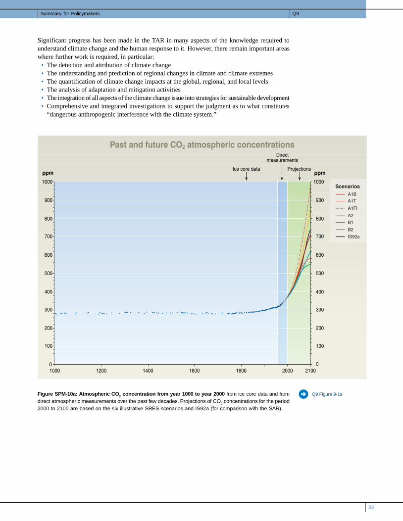
33
Summary for Policymakers
Significant progress has been made in the TAR in many aspects of the knowledge required tounderstand climate change and the human response to it. However, there remain important areaswhere further work is required, in particular:
The detection and attribution of climate changeThe understanding and prediction of regional changes in climate and climate extremesThe quantification of climate change impacts at the global, regional, and local levelsThe analysis of adaptation and mitigation activitiesThe integration of all aspects of the climate change issue into strategies for sustainable developmentComprehensive and integrated investigations to support the judgment as to what constitutes“dangerous anthropogenic interference with the climate system.”
••••••
Figure SPM-10a: Atmospheric CO2 concentration from year 1000 to year 2000 from ice core data and fromdirect atmospheric measurements over the past few decades. Projections of CO2 concentrations for the period2000 to 2100 are based on the six illustrative SRES scenarios and IS92a (for comparison with the SAR).
������������ ���51�������� �������� �����
���
'��
(��
���
)��
9��
���
���
����
���� ���� �(�� �)�� ���� ����
*�+*�,
*�-$
*�+�
+�
$.���
���� ���
����
���
'��
(��
���
)��
9��
���
���
����
���
�
��� ���
�
$�����������
8�����������������
/�2���������
Q9 Figure 9-1a
Q9

34
Climate Change 2001 Synthesis Report
IPCC Third Assessment Report
+�����#&�#�������������������0��������������� ���� �
.����� ���� �
� �.�3.����� 0�
���� ���� �(�� �)�� ���� ����
����
���
3� ��������������� �D���� ���������� ��� �7���� ��),,,����1),,
#��� �� ���������� ��� ����%��&� ������)<<,������'
���� �'�� ���� �9�� ���� ����
����
�����������4� ��#����"����0#���4�0�7������B ��
����������� ����������
/�2������
���
���
���
���
���
'��
'��
(��
(��
���
���
)��
*�+*�,
*�-$
*�+�
+�
$.���
���� ���
Figure SPM-10b: From year 1000 to year 1860 variations in average surface temperature of the NorthernHemisphere are shown (corresponding data from the Southern Hemisphere not available) reconstructedfrom proxy data (tree rings, corals, ice cores, and historical records). The line shows the 50-year average, thegrey region the 95% confidence limit in the annual data. From years 1860 to 2000 are shown variations inobservations of globally and annually averaged surface temperature from the instrumental record; the lineshows the decadal average. From years 2000 to 2100 projections of globally averaged surface temperatureare shown for the six illustrative SRES scenarios and IS92a using a model with average climate sensitivity.The grey region marked “several models all SRES envelope” shows the range of results from the full range of35 SRES scenarios in addition to those from a range of models with different climate sensitivities. Thetemperature scale is departure from the 1990 value; the scale is different from that used in Figure SPM-2.
Q9 Figure 9-1b

An Assessment of the Intergovernmental Panel on Climate Change
This underlying report, approved paragraph by paragraph at IPCC Plenary XVIII (Wembley, United Kingdom, 24-29 September 2001), represents the formally agreed statement of the IPCC concerning key findings and uncertainties contained in the Working Group contributions to the Third Assessment Report.
Climate Change 2001:Synthesis Report
Core Writing TeamRobert T. Watson, Daniel L. Albritton, Terry Barker, Igor A. Bashmakov, Osvaldo Canziani, Renate Christ, Ulrich Cubasch, Ogunlade Davidson, Habiba Gitay, David Griggs, John Houghton, Joanna House, Zbigniew Kundzewicz, Murari Lal, Neil Leary, Christopher Magadza, James J. McCarthy, John F.B. Mitchell, Jose Roberto Moreira, Mohan Munasinghe, Ian Noble, Rajendra Pachauri, Barrie Pittock, Michael Prather, Richard G. Richels, John B. Robinson, Jayant Sathaye, Stephen Schneider, Robert Scholes, Thomas Stocker, Narasimhan Sundararaman, Rob Swart, Tomihiro Taniguchi, and D. Zhou
Extended TeamQ.K. Ahmad, Oleg Anisimov, Nigel Arnell, Fons Baede, Tariq Banuri, Leonard Bernstein, Daniel H. Bouille, Timothy Carter, Catrinus J. Jepma, Liu Chunzhen, John Church, Stewart Cohen, Paul Desanker, William Easterling, Chris Folland, Filippo Giorgi, Jonathan Gregory, Kirsten Halsnaes, Joanna Haigh, Hideo Harasawa, Bruce Hewitson, Jean-Charles Hourcade, Mike Hulme, Tom Karl, Pekka E. Kauppi, Rik Leemans, Anil Markandya, Luis Jose Mata, Bryant McAvaney, Anthony McMichael, Linda Mearns, Jerry Meehl, Gylvan Meira-Filho, Evan Mills, William R. Moomaw, Berrien Moore, Tsuneyuki Morita, M.J. Mwandosya, Leonard Nurse, Martin Parry, Joyce Penner, Colin Prentice, Venkatachalam Ramaswamy, Sarah Raper, Jim Salinger, Michael Scott, Roger A. Sedjo, Priyaradshi R. Shukla, Barry Smit, Joel Smith, Leena Srivastava, Ron Stouffer, Kanako Tanaka, Ferenc L. Toth, Alla Tsyban, John P. Weyant, Tom Wilbanks, Francis Zwiers, and many IPCC authors
Review EditorsSusan Barrell, Rick Bradley, Eduardo Calvo, Ian Carruthers, Oyvind Christophersen, Yuri Izrael, Eberhard Jochem, Fortunat Joos, Martin Manning, Bert Metz, Alionne Ndiaye, Buruhani Nyenzi, Ramon Pichs-Madruga, Richard Odingo, Michel Petit, Jan Pretel, Armando Ramirez, Jose Romero, John Stone, R.T.M. Sutamihardja, David Warrilow, Ding Yihui, and John Zillman
Synthesis Report
Based on a draft prepared by:

Climate Change 2001:Synthesis Report
Synthesis Report
Synthesis Report
Question 1Question 2Question 3Question 4Question 5Question 6Question 7Question 8Question 9
Synthesis Report Tables
Synthesis Report Illustrations
35
37 40 47 57 61 68 74 84 91
99
116
Contents

PRE-PUBLICATION DRAFT IPCC SYNTHESIS REPORT TO THE TAR
Approved Synthesis Report Text 37 Subject to Final Copyedit
QUESTION 1
What can scientific, technical, and socio-economic analyses contribute to the determination of whatconstitutes dangerous anthropogenic interference with the climate system as referred to in Article 2 of theFramework Convention on Climate Change?
Box 1-1. Framework Convention on Climate Change, Article 2
“The ultimate objective of this Convention and any related legal instruments that the Conference of the Partiesmay adopt is to achieve, in accordance with the relevant provisions of the Convention, stabilization ofgreenhouse gas concentrations in the atmosphere at a level that would prevent dangerous anthropogenicinterference with the climate system. Such a level should be achieved within a time-frame sufficient to allowecosystems to adapt naturally to climate change, to ensure that food production is not threatened and to enableeconomic development to proceed in a sustainable manner.”
1.1 Natural, technical, and social sciences can provide essential information and evidence needed fordecisions on what constitutes “dangerous anthropogenic interference” with the climate system. At thesame time, such decisions are value judgments determined through socio-political processes, taking intoaccount considerations such as development, equity, and sustainability, as well as uncertainties and risk.Scientific evidence helps to reduce uncertainty and increase knowledge, and can serve as an input forconsidering precautionary measures.1 Decisions are based on risk assessment, and lead to risk managementchoices by decision makers, about actions and policies.2 [WGII TAR Section 2.7 & WGIII TAR Chapter10]
[FOOTNOTE 1: Conditions that justify the adoption of precautionary measures are described in Article 3.3of the United Nations Framework Convention on Climate Change (UNFCCC).]
[FOOTNOTE 2: The risk associated with an event is most simply defined as the probability of that event,multiplied by the magnitude of its consequence. Various decision frameworks can facilitate climate riskassessment and management. These include, among others, cost-benefit analysis, cost-effectivenessanalysis, multi-attribute analysis, and tolerable windows. Such techniques help to differentiate the risklevels associated with alternative futures, but in all cases the analyses are marked by considerableuncertainties.]
1.2 The basis for determining what constitutes “dangerous anthropogenic interference” will vary amongregions—depending both on the local nature and consequences of climate change impacts, and also onthe adaptive capacity available to cope with climate change—and depends upon mitigative capacity,since the magnitude and the rate of change are both important. The consequent types of adaptationresponses that will be selected depend on the effectiveness of various adaptation or mitigation responses inreducing vulnerabilities and improving the sustainability of life-support systems. There is no universallyapplicable best set of policies; rather, it is important to consider both the robustness of different policymeasures against a range of possible future worlds, and the degree to which such climate-specific policiescan be integrated with broader sustainable development policies. [WGII TAR Chapter 18 & WGIII TARChapter 10]
1.3 The Third Assessment Report (TAR) provides an assessment of new scientific information and evidenceas an iput for policy makers in their determination of what constitutes “dangerous anthropogenicinterference with the climate system” with regard to: (1) the magnitudes and rates of changes in theclimate system, (2) the ecological and socio-economic impacts of climate change, and (3) the potential forachieving a broad range of levels of concentrations through mitigation and information about howadaptation can reduce vulnerability. [WGI TAR, WGII TAR, & WGIII TAR]

PRE-PUBLICATION DRAFT IPCC SYNTHESIS REPORT TO THE TAR
Approved Synthesis Report Text 38 Subject to Final Copyedit
1.4 With regard to the magnitudes and rates of changes in the climate system, the TAR provides scenario-based projections of future concentrations of greenhouse gases in the atmosphere, global and regionalpatterns of changes and rates of change in temperature, precipitation, and sea level, and changes inextreme climate events. It also examines possibilities for abrupt and irreversible changes in oceancirculation and the major ice sheets. [WGI TAR]
1.5 The TAR reviews the biophysical and socio-economic impacts of climate change. The TAR articulatesfive reasons for concern, regarding:• Risks to unique and threatened systems• Risks associated with extreme weather events• The distribution of impacts• Aggregate impacts• Risks of large-scale, high-impact events.Of great significance here is an assessment of the likelihood of the critical thresholds at which natural andhuman systems exhibit large-scale, abrupt, or irreversible changes in their response to a changing climate.Since no single indicator (e.g., a monetary unit) captures the range of relevant risks presented by climatechange, a variety of analytical approaches and criteria are required to assess impacts and facilitate decisionsabout risk management. [WGII TAR Chapter 19]
1.6 With regard to strategies for addressing climate change, the TAR provides an assessment of the potentialfor achieving different levels of concentrations through mitigation and information about howadaptation can reduce vulnerability. The causality works in both directions. Different stabilization levelsresult from different emission scenarios, which are connected to underlying development paths. In turn,these development paths strongly affect adaptive capacity in any region. In this way adaptation andmitigation strategies are dynamically connected with changes in the climate system and the prospects forecosystem adaptation, food production, and sustainable economic development. [WGII TAR Chapter 18 &WGIII TAR Chapter 2]
1.7 An integrated view of climate change considers the dynamics of the complete cycle of interlinked causesand effects across all sectors concerned. Figure 1-1 shows the cycle, from the underlying driving forces ofpopulation, economy, technology, and governance, through greenhouse gas and other emissions, changes inthe physical climate system, biophysical and human impacts, to adaptation and mitigation, and back to thedriving forces. The figure presents a schematic view of an ideal “integrated assessment” framework, inwhich all the parts of the climate change problem interact mutually. Changes in one part of the cycleinfluence other components in a dynamic manner, through multiple paths. The TAR assesses new policy-relevant information and evidence with regard to all quadrants of Figure 1-1. In particular, a newcontribution has been to fill in the bottom righthand quadrant of the figure by exploring alternativedevelopment paths and their relationship to greenhouse gas emissions, and by undertaking preliminarywork on the linkage between adaptation, mitigation, and development paths. However, the TAR does notachieve a fully integrated assessment of climate change, because of the incomplete state of knowledge.[WGII TAR Chapters 1 & 19, WGIII TAR Chapter 1, & SRES]
[FIGURE 1-1 CAPTION: Schematic and simplified representation of an integrated assessment frameworkfor considering anthropogenic climate change. The yellow arrows show a full clockwise cycle of cause andeffect among the four quadrants shown in the figure, while the blue arrow indicates the societal response toclimate change impacts. For both developed and developing countries, each socio-economic developmentpath explored in the Special Report on Emissions Scenarios has driving forces which give rise to emissionsof greenhouse gases, aerosols, and precursors—with carbon dioxide (CO2) being the most important. Thegreenhouse gas emissions accumulate in the atmosphere, changing concentrations and disturbing thenatural balances, depending on physical processes such as solar radiation, cloud formation, and rainfall.The aerosols also give rise to air pollution (e.g., acid rain) that damage human and the natural systems (notshown). The enhanced greenhouse effect will initiate climate changes well into the future with associatedimpacts on the natural and human systems. There is a possibility of some feedback between the changesin these systems and the climate (not shown), such as albedo effects from changing land use, and other,perhaps larger, interactions between the systems and atmospheric emissions (e.g., effects of changes in landuse (again not shown)). These changes will ultimately have effects on socio-economic development paths.
PRE-PUBLICATION DRAFT IPCC SYNTHESIS REPORT TO THE TAR
Approved Synthesis Report Text 39 Subject to Final Copyedit
The development paths also have direct effects on the natural systems (shown by the anti-clockwise arrowfrom the development box) such as changes in land use leading to deforestation. This figure illustrates thatthe various dimensions of the climate change issue exist in a dynamic cycle, characterized by significanttime delays. Both emissions and impacts, for example, are linked in complex ways to underlying socio-economic and technological development paths. A major contribution of the TAR has been to explicitlyconsider the bottom righthand domain (shown as a rectangle) by examining the relationships betweengreenhouse gas emissions and development paths (in SRES), and by assessing preliminary work on thelinkage between adaptation, mitigation, and development paths (WGII and WGIII). However, the TARdoes not achieve a fully integrated assessment of climate change, since not all components of the cyclewere able to be linked dynamically. Adaptation and mitigation are shown as modifying the effects shown inthe figure.]
1.8 Climate change decision making is essentially a sequential process under general uncertainties. Decisionmaking has to deal with uncertainties including the risk of non-linear and/or irreversible changes andentails balancing the risk of either insufficient or excessive action, and involves careful consideration of theconsequences (both environmental and economic), their likelihood, and society’s attitude towards risk. Thelatter is likely to vary from country to country and from generation to generation. The relevant question is“what is the best course for the near term given the expected long-term climate change and accompanyinguncertainties.” [WGI TAR, WGII TAR, & WGIII TAR Section 10.1.4]
1.9 Climate change impacts are part of the larger question of how complex social, economic, andenvironmental subsystems interact and shape prospects for sustainable development. There are multiplelinks. Economic development affects ecosystem balance and, in turn, is affected by the state of theecosystem; poverty can be both a result and a cause of environmental degradation; material- and energy-intensive life styles and continued high levels of consumption supported by non-renewable resources andrapid population growth are not likely to be consistent with sustainable development paths; and extremesocio-economic inequality within communities and between nations may undermine the social cohesionthat would promote sustainability and make policy responses more effective. At the same time, socio-economic and technology policy decisions made for non-climate-related reasons have significantimplications for climate policy and climate change impacts, as well as for other environmental issues (seeQuestion 8). In addition, critical impact thresholds and vulnerability to climate change impacts are directlyconnected to environmental, social, and economic conditions and institutional capacity. [WGII TAR]
1.10 As a result, the effectiveness of climate policies can be enhanced when they are integrated with broaderstrategies designed to make national and regional development paths more sustainable. This occursbecause of the impacts of natural climate variation and changes, climate policy responses, and associatedsocio-economic development will affect the ability of countries to achieve sustainable development goals,while the pursuit of those goals will in turn affect the opportunities for, and success of, climate policies. Inparticular, the socio-economic and technological characteristics of different development paths willstrongly affect emissions, the rate and magnitude of climate change, climate change impacts, the capabilityto adapt, and the capacity to mitigate climate. The Special Report on Emissions Scenarios (SRES, see Box3-1) outlined multiple plausible future worlds with different characteristics, each having very differentimplications for the future climate and for climate policy. [WGIII TAR Section 10.3.2]
1.11 The TAR assesses available information on the timing, opportunities, costs, benefits, and impacts ofvarious mitigation and adaptation options. It indicates that there are opportunities for countries actingindividually, or in cooperation with others, to reduce costs of mitigation and adaptation and realize benefitsassociated with achieving sustainable development. [WGII TAR Chapter 18, WGIII TAR Chapters 8, 9, &10, & SRES]

PRE-PUBLICATION DRAFT IPCC SYNTHESIS REPORT TO THE TAR
Approved Synthesis Report Text 40 Subject to Final Copyedit
QUESTION 2
What is the evidence for, causes of, and consequences of changes in the Earth’s climate since the pre-industrial era? (a) Has the Earth’s climate changed since the pre-industrial era at the regional and/or globalscale? If so, what part, if any, of the observed changes can be attributed to human influence and what part, ifany, can be attributed to natural phenomena? What is the basis for that attribution? (b) What is knownabout the environmental, social, and economic consequences of climate changes since the pre-industrial erawith an emphasis on the last 50 years?
2.1 This answer focuses on classical measures of climate (e.g., temperature, precipitation, sea level, plusextreme events including floods, droughts, and storms), on other components of the Earth’s climate system(e.g., greenhouse gases and aerosols, ecological systems), and on human health and socio-economicsectors. Climate change as defined in IPCC refers to statistically significant variations that persist for anextended period, typically decades or longer. It includes shifts in the frequency and magnitude of sporadicweather events as well as the slow continuous rise in global mean surface temperature. Thus the discussionhere includes climate-weather variations on all temporal and spatial scales, ranging from brief-lived severestorms to seasonal El Niño events, decadal droughts, and century shifts in temperature and ice cover.Although short-term climate variations are considered predominantly natural at present, their impacts arediscussed in this question because they represent a class of changes that may become more prevalent in afuture climate perturbed by human activities (see Question 4). Attribution is used here as the process ofestablishing the most likely causes for the detected change with some defined level of confidence. Thediscussion includes both climate change that is attributable to human influence and climate change that mayat present be natural but might in the future be modified through human influence (see Box 3-1).
2.2 The Earth’s climate system has demonstrably changed on both global and regional scales since thepre-industrial era, with some of these changes attributable to human activities.
2.3 Emissions of greenhouse gases and aerosols due to human activities continue to alter the atmospherein ways that are expected to affect the climate (see Table 2-1).
[Insert Table 2-1 here]
2.4 Concentrations of atmospheric greenhouse gases and their radiative forcings have generally increasedover the 20th century as a result of human activities. Almost all greenhouse gases reached their highestrecorded levels in the 1990s and continue to increase (see Figure 2-1). Atmospheric carbon dioxide (CO2)and methane (CH4) have varied substantially during glacial-interglacial cycles over the past 420,000 years,but even the largest of these earlier values are much less than their current atmospheric concentrations. Interms of radiative forcing by greenhouse gases emitted through human activity, CO2 and CH4 are the firstand second most important, respectively. From the years 1750 to 2000, the concentration of CO2 increasedby 31±4%, and that of CH4 rose by 151±25% (see Box 2-1 and Figure 2-1). These rates of increase areunprecedented. Fossil-fuel burning released on average 5.4 Gt C yr-1 during the 1980s, increasing to 6.3 GtC yr-1 during the 1990s. About three-quarters of the increase in atmospheric CO2 during the 1990s wascaused by fossil-fuel burning, with land-use change including deforestation responsible for the rest. Overthe 19th and much of the 20th century the terrestrial biosphere has been a net source of atmospheric CO2,but before the end of the 20th century it had become a net sink. The increase in CH4 can be identified withemissions from energy use, livestock, rice agriculture, and landfills. Increases in the concentrations of othergreenhouse gases-particularly tropospheric ozone (O3), the third most important-are directly attributable tofossil-fuel combustion as well as other industrial and agricultural emissions. [WGI TAR Chapters 3 & 4, &SRAGA]
[Box 2-1: Confidence and likelihood statements. Where appropriate, the authors of the Third AssessmentReport assigned confidence levels that represent their collective judgment in the validity of a conclusionbased on observational evidence, modeling results, and theory that they have examined. The followingwords have been used throughout the text of the Synthesis Report to the TAR relating to WGI findings:

PRE-PUBLICATION DRAFT IPCC SYNTHESIS REPORT TO THE TAR
Approved Synthesis Report Text 41 Subject to Final Copyedit
virtually certain (greater than 99% chance that a result is true); very likely (90–99% chance); likely(66–90% chance); medium likelihood (33–66% chance); unlikely (10–33% chance); very unlikely (1–10%chance); and exceptionally unlikely (less than 1% chance). An explicit uncertainty range (±) is a likelyrange. Estimates of confidence relating to WGII findings are: very high (95% or greater), high (67–95%),medium (33–67%), low (5–33%), and very low (5% or less). No confidence levels were assigned in WGIII.][WGI TAR SPM & WGII TAR SPM]
[FIGURE 2-1 CAPTION: Records of past changes in atmospheric composition over the last millenniumdemonstrate the rapid rise in greenhouse gases and sulfate aerosols that is attributable primarily toindustrial growth since 1750. The top three panels show increasing atmospheric concentrations of carbondioxide (CO2), methane (CH4), and nitrous oxide (N2O) over the past 1,000 years. Early sporadic data takenfrom air trapped in ice (symbols) matches up with continuous atmospheric observations from recentdecades (solid lines). These gases are well mixed in the atmosphere, and their concentrations reflectemissions from sources throughout the globe. The estimated positive radiative forcing from these gases isindicated on the righthand scale. The lowest panel shows the concentration of sulfate in ice cores fromGreenland (shown by lines for three different cores) from which the episodic effects of volcanic eruptionshave been removed. Sulfate aerosols form from sulfur dioxide (SO2) emissions, deposit readily at thesurface, and are not well mixed in the atmosphere. Specifically, the increase in sulfate deposited atGreenland is attributed to SO2 emissions from the U.S. and Europe (shown as symbols), and both show adecline in recent decades. Sulfate aerosols produce negative radiative forcing.] [WGI TAR Figures SPM-2,3-2b, 4-1a, 4-1b, 4-2, & 5.4a]
2.5 The radiative forcing from the increase in anthropogenic greenhouse gases since the pre-industrial erais positive (warming) with a small uncertainty range; that from the direct effects of aerosols is negative(cooling) and smaller; whereas the negative forcing from the indirect effects of aerosols (on clouds andthe hydrologic cycle) might be large but is not well quantified. Key anthropogenic and natural factorscausing a change in radiative forcing from year 1750 to year 2000 are shown in Figure 2-2, where thefactors whose radiative forcing can be quantified are marked by wide, colored bars. Only some of theaerosol effects are estimated here and denoted as ranges. Other factors besides atmosphericconstituents—solar irradiance and land-use change—are also shown. Stratospheric aerosols from largevolcanic eruptions have led to important, but brief-lived, negative forcings (particularly the periods1880–1920 and 1960–1994), which are not important over the time scale since the pre-industrial era andnot shown. The sum of quantified factors in Figure 2-2 (greenhouse gases, aerosols and clouds, land-use(albedo), and solar irradiance) is positive, but this does not include the potentially large, negative forcingfrom aerosol indirect effects. The total change in radiative forcing since the pre-industrial era continues tobe a useful tool to estimate, to a first order, the global mean surface temperature response to human andnatural perturbations; however, the sum of forcings is not necessarily an indicator of the detailed aspects ofthe potential climate responses such as regional climate change. For the last half of the 20th century (notshown), the positive forcing due to well-mixed greenhouse gases has increased rapidly over the past 4decades, while in contrast the sum of natural forcings has been negative over the past 2 and possibly even 4decades. [WGI TAR Chapter 5 & 6, & SRAGA Chapter 6]
[FIGURE 2-2 CAPTION: The influence of external factors on climate can be broadly compared using theconcept of radiative forcing. These radiative forcings arise from changes in the atmospheric composition,alteration of surface reflectance by land use, and variation in the output of the sun. Except for solarvariation, some form of human activity is linked to each. The rectangular bars represent estimates of thecontributions of these forcings, some of which yield warming and some cooling. Forcing due to episodicvolcanic events, which lead to a negative forcing lasting only for a few years, is not shown. The indirecteffect of aerosols shown is their effect on the size and number of cloud droplets. A second indirect effect ofaerosols on clouds, namely their effect on cloud lifetime, which would also lead to a negative forcing, is notshown. Effects of aviation on greenhouse gases are included in the individual bars. The vertical line aboutthe rectangular bars indicates a range of estimates, guided by the spread in the published values of theforcings and physical understanding. Some of the forcings possess a much greater degree of certainty thanothers. A vertical line without a rectangular bar denotes a forcing for which no best estimate can be givenowing to large uncertainties. The overall level of scientific understanding for each forcing variesconsiderably, as noted. Some of the radiative forcing agents are well mixed over the globe, such as CO2,

PRE-PUBLICATION DRAFT IPCC SYNTHESIS REPORT TO THE TAR
Approved Synthesis Report Text 42 Subject to Final Copyedit
thereby perturbing the global heat balance. Others represent perturbations with stronger regional signaturesbecause of their spatial distribution, such as aerosols. Radiative forcing continues to be a useful tool toestimate, to a first order, the relative climate impacts such as the relative global mean surface temperatureresponse due to radiatively induced perturbations, but these global mean forcing estimates are notnecessarily indicators of the detailed aspects of the potential climate responses (e.g., regional climatechange).] [WGI TAR SPM, WGI TAR Chapter 6 ES, & WGI TAR Figures SPM-3 & 6-6]
2.6 An increasing body of observations gives a collective picture of a warming world and other changesin the climate system (see Table 2-1).
2.7 The global average surface temperature has increased from the 1860s to the year 2000, the period ofinstrumental record. Over the 20th century this increase was 0.6°C with a very likely (see Box 2-1)confidence range of 0.4–0.8°C (see Figure 2-3a). It is very likely that the 1990s was the warmest decade,and 1998 the warmest year, of the instrumental record. Extending the instrumental record with proxy datafor the Northern Hemisphere indicates that over the past 1,000 years the 20th century increase intemperature is likely to have been the largest of any century, and the 1990s was likely the warmest decade(see Figure 2-3b). Insufficient data are available in the Southern Hemisphere prior to the year 1860 tocompare the recent warming with changes over the last 1,000 years. Since the year 1950, the increase in seasurface temperature is about half that of the mean land surface air temperature. During this period thenighttime daily minimum temperatures over land have increased on average by about 0.2°C per decade,about twice the corresponding rate of increase in daytime maximum air temperatures. These climatechanges have lengthened the frost-free season in many mid- and high-latitude regions. [WGI TAR SPM &WGI TAR Chapter 2]
[FIGURE 2-3 CAPTION: The Earth’s surface temperature has increased by about 0.6oC over the record ofdirect temperature measurements (1860–2000, top panel)—a rise that is unprecedented, at least based onproxy temperature data for the Northern Hemisphere, over the last millennium (bottom panel). In the toppanel the global mean surface temperature is shown year-by-year (red bars with very likely ranges as thinblack whiskers) and approximately decade-by-decade (continuous red line). Analyses take into accountdata gaps, random instrumental errors and uncertainties, uncertainties in bias corrections in the oceansurface temperature data, and also in adjustments for urbanization over the land. The lower panel mergesproxy data (year-by-year blue line with very likely ranges as grey band, 50-year-average purple line) andthe direct temperature measurements (red line) for the Northern Hemisphere. The proxy data consist of treerings, corals, ice cores, and historical records that have been calibrated against thermometer data.Insufficient data are available to assess such changes in the Southern Hemisphere.] [WGI TAR FiguresSPM-1, 2-7c, & 2-20]
2.8 In the lowest 8 km of the atmosphere the global temperature increase from the 1950s to the year 2000,about 0.1°C per decade, has been similar to that at the surface. For the period 1979–2000 both satelliteand weather balloon measurements show nearly identical warming over North America (0.3oC per decade)and Europe (0.4oC per decade) for both surface and lower atmosphere, but distinct differences over someland areas and particularly in the tropical regions (0.10±0.10°C per decade for surface versus 0.06±0.16°Cper decade for the lower atmosphere). Temperatures of the surface and lower atmosphere are influenceddifferently by factors such as stratospheric ozone depletion, atmospheric aerosols, and the El Niñophenomenon. In addition, spatial sampling techniques can also explain some of the differences in trends,but these differences are not fully resolved. [WGI TAR SPM & WGI TAR Section 2.2.4]
2.9 There is new and stronger evidence that most of the warming observed over the last 50 years isattributable to human activities.
2.10 The observed warming over the 20th century is unlikely to be entirely natural in origin. The increase insurface temperatures over the last 100 years is very unlikely to be due to internal variability alone.Reconstructions of climate data for the last 1,000 years also indicate that this 20th century warming wasunusual and unlikely to be the response to natural forcing alone: That is, volcanic eruptions and variation insolar irradiance do not explain the warming in the latter half of the 20th century (see Figure 2-4a), but theymay have contributed to the observed warming in the first half. [WGI TAR SPM & WGI TAR Chapter 12]

PRE-PUBLICATION DRAFT IPCC SYNTHESIS REPORT TO THE TAR
Approved Synthesis Report Text 43 Subject to Final Copyedit
[FIGURE 2-4 CAPTION: Simulating the Earth’s temperature variations and comparing the results to themeasured changes can provide insight into the underlying causes of the major changes. A climate modelcan be used to simulate the temperature changes that occur from both natural and anthropogenic causes.The simulations represented by the band in (a) were done with only natural forcings: solar variation andvolcanic activity. Those encompassed by the band in (b) were done with anthropogenic forcings:greenhouse gases and an estimate of sulfate aerosols. Those encompassed by the band in (c) were donewith both natural and anthropogenic forcings included. From (b), it can be seen that the inclusion ofanthropogenic forcings provides a plausible explanation for a substantial part of the observed temperaturechanges over the past century, but the best match with observations is obtained in (c) when both natural andanthropogenic factors are included. These results show that the forcings included are sufficient to explainthe observed changes, but do not exclude the possibility that other forcings may also have contributed.Similar results to those in (b) are obtained with other models with anthropogenic forcing.] [WGI TARFigure 12-7]
2.11 In the light of new evidence and taking into account the remaining uncertainties, most of the observedwarming over the last 50 years is likely to have been due to the increase in greenhouse gasconcentrations. Detection and attribution studies (including greenhouse gases and sulfate aerosols asanthropogenic forcing) consistently find evidence for an anthropogenic signal in the climate record of thelast 35 to 50 years, despite uncertainties in forcing due to anthropogenic sulfate aerosols and natural factors(volcanoes and solar irradiance). The sulfate and natural forcings are negative over this period and cannotexplain the warming (see Figure 2-4a); whereas most of these studies find that, over the last 50 years, theestimated rate and magnitude of warming due to increasing greenhouse gases alone are comparable with, orlarger than, the observed warming (Figure 2-4b). The best agreement for the 1860–2000 record is foundwhen the above anthropogenic and natural forcing factors are combined (see Figure 2-4c). This result doesnot exclude the possibility that other forcings may also contribute, and some known anthropogenic factors(e.g., organic carbon, black carbon (soot), biomass aerosols, and some changes in land use) have not beenused in these detection and attribution studies. Estimates of the magnitude and geographic distribution ofthese additional anthropogenic forcings vary considerably. [WGI TAR SPM & WGI TAR Chapter 12]
2.12 Changes in sea level, snow cover, ice extent, and precipitation are consistent with a warming climatenear the Earth’s surface (see Table 2-1). Some of these changes are regional and some may be due tointernal climate variations, natural forcings, or regional human activities rather than attributed solely toglobal human influence.
2.13 It is very likely that the 20th century warming has contributed significantly to the observed rise in globalaverage sea level and increase in ocean-heat content. Warming drives sea-level rise through thermalexpansion of seawater and widespread loss of land ice. Based on tide gauge records, after correcting forland movements, the average annual rise was between 1 and 2 mm during the 20th century. The very fewlong records show that it was less during the 19th century (see Figure 2-5). Within present uncertainties,observations and models are both consistent with a lack of significant acceleration of sea-level rise duringthe 20th century. The observed rate of sea-level rise during the 20th century is consistent with models.Global ocean-heat content has increased since the late 1950s, the period with adequate observations ofsubsurface ocean temperatures. [WGI TAR Sections 2.2.2.5, 11.2.1, & 11.3.2]
[FIGURE 2-5 CAPTION: A limited number of sites in Europe have nearly continuous records of sea levelspanning 300 years and show the greatest rise in sea level over the 20th century. Records shown fromAmsterdam, The Netherlands, Brest, France, and Swinoujscie, Poland, as well as other sites, confirm theaccelerated rise in sea level over the 20th century as compared to the 19th.] [WGI TAR Figure 11-7]
2.14 Snow cover and ice extent have decreased. It is very likely that the extent of snow cover has decreased byabout 10% on average in the Northern Hemisphere since the late 1960s (mainly through springtime changesover America and Eurasia) and that the annual duration of lake- and river-ice cover in the mid- and highlatitudes of the Northern Hemisphere has been reduced by about 2 weeks over the 20th century. There hasalso been a widespread retreat of mountain glaciers in non-polar regions during the 20th century. It is likelythat Northern Hemisphere spring and summer sea-ice extent has decreased by about 10 to 15% from the

PRE-PUBLICATION DRAFT IPCC SYNTHESIS REPORT TO THE TAR
Approved Synthesis Report Text 44 Subject to Final Copyedit
1950s to the year 2000 and that Arctic sea-ice thickness has declined by about a 40% during late summerand early autumn in the last 3 decades of the 20th century. While there is no change in overall Antarcticsea-ice extent from 1978 to 2000 in parallel with global mean surface temperature increase, regionalwarming in the Antarctic Peninsula coincided with the collapse of the Prince Gustav and parts of the Larsenice shelves during the 1990s, but the loss of these ice shelves has had little direct impact. [WGI TARChapter 2]
2.15 Precipitation has very likely increased during the 20th century by 5 to 10% over most mid- and highlatitudes of the Northern Hemisphere continents, but in contrast, rainfall has likely decreased by 3% onaverage over much of the subtropical land areas (see Figure 2-6a). Increasing global mean surfacetemperature is very likely to lead to changes in precipitation and atmospheric moisture because of changesin atmospheric circulation, a more active hydrologic cycle, and increases in the water-holding capacitythroughout the atmosphere. There has likely been a 2 to 4% increase in the frequency of heavy precipitationevents in the mid- and high latitudes of the Northern Hemisphere over the latter half of the 20th century.There were relatively small long-term increases over the 20th century in land areas experiencing severedrought or severe wetness, but in many regions these changes are dominated by inter-decadal and multi-decadal climate variability with no significant trends evident over the 20th century. [WGI TAR Sections2.5, 2.7.2.2, & 2.7.3]
[FIGURE 2-6a CAPTION: Precipitation during the 20th century has on average increased over continentsoutside the tropics but decreased in the desert regions of Africa and South America. While the recordshows an overall increase consistent with warmer temperatures and more atmospheric moisture, trends inprecipitation vary greatly from region to region and are only available over the 20th century for somecontinental regions. Over this period, there were relatively small long-term trends in land areasexperiencing severe drought or severe wetness, but in many regions these changes are dominated by inter-decadal and multi-decadal climate variability that has no trends evident over the 20th century.] [[WGI TARFigure 2-25]
2.16 Changes have also occurred in other important aspects of climate (see Table 2-1).
2.17 Over the 20th century there has been a consistent, large-scale warming of both the land and oceansurface, with largest increases in temperature over the mid- and high latitudes of northern continents.The warming of land surface faster than ocean surface from the years 1976 to 2000 (see Figure 2-6b) isconsistent both with the observed changes in natural climate variations, such as the North Atlantic andArctic Oscillations, and with the modeled pattern of greenhouse gas warming. As described below,statistically significant associations between regional warming and observed changes in biological systemshave been documented in freshwater, terrestrial, and marine environments on all continents. [WGI TARSection 2.2.2.4 & WGII TAR Sections 5.2.1, 5.4, & 6.3]
[FIGURE 2-6b CAPTION: A consistent, large-scale warming of both the land and ocean surface occurredover the last quarter of the 20th century, with largest temperature increases over the mid- and high latitudesof North America, Europe, and Asia. Large regions of cooling occurred only in parts of the Pacific andSouthern Oceans and Antarctica. The warming of land faster than ocean surface could be in part a signal ofanthropogenic warming; however, a component of the pattern of warming at northern mid-latitudes appearsto be related to natural climate variations such as the North Atlantic and Arctic Oscillations. As describedin the text, warming in some regions is linked with observed changes in biological systems on allcontinents.] [WGI TAR Figure 2-9d]
2.18 Warm episodes of the El NiñoSouthern Oscillation (ENSO) phenomenon have been more frequent,persistent, and intense since the mid-1970s, compared with the previous 100 years. ENSO consistentlyaffects regional variations of precipitation and temperature over much of the tropics, subtropics, and somemid-latitude areas. It is not obvious from models, however, that a warmer world would have a greaterfrequency of occurrence of El Niño events. [WGI TAR Sections 2.6.2 & 9.3.5.2]
2.19 Some important aspects of climate appear not to have changed. A few areas of the globe have not warmedin recent decades, mainly over some parts of the Southern Hemisphere oceans and parts of Antarctica (see

PRE-PUBLICATION DRAFT IPCC SYNTHESIS REPORT TO THE TAR
Approved Synthesis Report Text 45 Subject to Final Copyedit
Figure 2-6b). There are no demonstrated changes in overall Antarctic sea-ice extent since 1978, the periodof reliable satellite measurements. Current analyses are unable to draw conclusions about the likelihood ofchanges in the frequency of tornadoes, thunder days, or hail events for the limited regions that have beenstudied. In addition, insufficient data and conflicting analyses prevent an assessment of changes inintensities of tropical and extra-tropical cyclones and severe local storm activity in the mid-latitudes. [WGITAR Sections 2.2.2, 2.2.5, & 2.7.3]
2.20 Observed changes in regional climate over the past 50 years have affected biological and hydrologicalsystems in many parts of the world (see Table 2-1).
2.21 There has been a discernible impact of regional climate change, particularly increases in temperature,on biological systems in the 20th century. In many parts of the world the observed changes in thesesystems3, either anthropogenic or natural, are coherent across diverse localities and are consistent indirection with the expected effects of regional changes in temperature. The probability that the observedchanges in the expected direction (with no reference to magnitude) could occur by chance alone isnegligible. Such systems include, for example, species distributions, population sizes, and the timing ofreproduction or migration events. These observations implicate regional climate change as a prominentcontributing causal factor. There have been observed changes in the types (e.g., fires, droughts,blowdowns), intensity, and frequency of disturbances that are affected by regional climatic change (eitheranthropogenic or natural) and land-use practices, and they in turn affect the productivity of and speciescomposition within an ecosystem, particularly at high latitudes and high altitudes. Frequency of pests anddisease outbreaks have also changed, especially in forested systems, and can be linked to changes inclimate. In some regions of Africa, the combination of regional climate changes (Sahelian drought) andanthropogenic stresses has led to decreased cereal crop production since the year 1970. There are somepositive aspects of warming: For example, the growing season across Europe has lengthened by about 11days from the years 1959 to 1993, and energy consumption for heating in winter has decreased. [WGIITAR Sections 5.4, 5.6.2, 10.1.3.2, 13.1.3.1, & 13.2.4.1, & WGII TAR Figure SPM-1]
[FOOTNOTE 3: There are 44 regional studies of over 400 plants and animals, which varied in length fromabout 20 to 50 years, mainly from North America, Europe, and the southern polar region. There are 16regional studies covering about 100 physical processes over most regions of the world, which varied inlength from about 20 to 150 years.]
2.22 Coral reefs are adversely affected by rising sea surface temperatures. Increasing sea surface temperatureshave been recorded in much of the tropical oceans over the past several decades. Many corals haveundergone major, although often partially reversible, bleaching episodes when sea surface temperatures riseby 1°C in any one season, and extensive mortality occurs for a 3°C rise. This typically occurs during ElNiño events and is exacerbated by rising sea surface temperatures. These bleaching events are oftenassociated with other stresses such as pollution. [WGII TAR Section 6.4.5]
2.23 Changes in marine systems, particularly fish populations, have been linked to large-scale climateoscillations. The El Niño affects fisheries off the coasts of South America and Africa and the decadaloscillations in the Pacific are linked to decline of fisheries off the west coast of North America. [WGI TARSection 2.6.3 & WGII TAR Sections 14.1.3 & 15.2.3.3]
2.24 Changes in stream flow, floods, and droughts have been observed. Evidence of regional climate changeimpacts on elements of the hydrological cycle suggest that warmer temperatures lead to intensification ofthe hydrological cycle. Peak stream flow has shifted back from spring to late winter in large parts of easternEurope, European Russia, and North America in the last decades. The increasing frequency of droughts andfloods in some areas is related to variations in climate—for example, droughts in Sahel and in northeast andsouthern Brazil, and floods in Colombia and northwest Peru. [WGI TAR Section 2.7.3.3, WGII TAR SPM,WGII TAR Sections 4.3.6, 14.3, & 19.2.2.1, & WGII TAR Table 4-6]
2.25 There are preliminary indications that social and economic systems have been affected by observedchanges in regional climate. The rising socio-economic costs related to weather damage and toregional variations in climate suggest increasing vulnerability to climate change (see Table 2-1).

PRE-PUBLICATION DRAFT IPCC SYNTHESIS REPORT TO THE TAR
Approved Synthesis Report Text 46 Subject to Final Copyedit
2.26 Extreme weather or climatic events cause substantial, and increasing, damage. Extreme events arecurrently a major source of climate-related impacts. For example, heavy losses of human life, propertydamage, and other environmental damages were recorded during the El Niño event of the years 1997–1998.The impacts of climatic extremes and variability are a major concern. Preliminary indications suggest thatsome social and economic systems have been affected by recent increases in floods and droughts, withincreases in economic losses for catastrophic weather events. Because these systems are also affected bychanges in socio-economic factors such as demographic shifts and land-use changes, quantifying therelative impacts of climate change (either anthropogenic or natural) and of socio-economic factors isdifficult. For example, direct costs of global catastrophic weather-related losses, corrected for inflation,have risen an order of magnitude from the 1950s to the 1990s (see Figure 2-7), and costs for non-catastrophic weather events have grown similarly. The number of weather-related catastrophic events hasrisen three times faster than the number of non-weather-related events, despite generally enhanced disasterpreparedness. Part of this observed upward trend in weather-related losses over the past 50 years is linkedto regional socio-economic factors (e.g., population growth, increased wealth, urbanization in vulnerableareas), and part is linked to climatic factors (e.g., changes in precipitation, flooding events). [WGII TARSPM & WGII TAR Section 8.2]
[FIGURE 2-7 CAPTION: The economic losses from catastrophic weather events have risen globally 10-fold (inflation-adjusted) from the 1950s to the 1990s, much faster than can be accounted for with simpleinflation. The insured portion of these losses rose from a negligible level to about 23% in the 1990s. Thetotal losses from small, non-catastrophic weather-related events (not included here) are similar. Part of thisobserved upward trend in weather-related disaster losses over the past 50 years is linked to socio-economicfactors (e.g., population growth, increased wealth, urbanization in vulnerable areas), and part is linked toclimatic regional factors (e.g., changes in precipitation, flooding events).] [WGII TAR Figure 8-1]
2.27 The fraction of weather-related losses covered by insurance varies considerably by region, and theuneven impacts of climatic hazards raise issues for development and equity. Insurers pay only 5% of totaleconomic losses today in Asia and South America, 10% in Africa, and about 30% in Australia, Europe, andNorth and Central America. The fraction covered is typically much higher when just storm losses areconsidered, but flood- and crop-related losses have much lower coverage. The balance of the losses areabsorbed by governments and affected individuals and organizations. [WGII TAR Section 8.3.3.1]
2.28 Climate-related health effects are observed. Many vector-, food-, and water-borne infectious diseases areknown to be sensitive to changes in climatic conditions. Extensive experience makes clear that any increasein floods will increase the risk of drowning, diarrheal and respiratory diseases, water-contaminationdiseases, and-in developing countries-hunger and malnutrition (high confidence). Heat waves in Europeand North America are associated with a significant increase in urban mortality, but warmer wintertimetemperatures also result in reduced wintertime mortality. In some cases health effects are clearly related torecent climate changes, such as in Sweden where tick-borne encephalitis incidence increased after milderwinters and moved northward following the increased frequency of milder winters over the years 1980 to1994. [WGII TAR SPM & WGII TAR Sections 9.5.1, 9.7.8, & 13.2.5]
2.29 The recognition and anticipation of adverse impacts of climate change has led to both public andgovernmental responses.
2.30 As a consequence of observed and anticipated climate change, socio-economic and policy responseshave occurred in the last decade. These have included stimulation of the renewable energy market,development of energy-efficiency improvement programs enhanced by climate change concerns,integration of climate policies into broader national policies, carbon taxes in several countries, domesticgreenhouse gases trading regimes in some countries, national and international voluntary agreements withindustries to increase energy efficiency or otherwise decrease greenhouse gas emissions, creation of carbonexchange markets, public and political pressures for utilities to reduce or offset carbon emissions from newenergy projects, industry reconnaissance into approaches to offset carbon emissions, and establishment ofprograms to assist the developing and least developed countries reduce vulnerabilities and adapt to climatechange and engage in mitigation activities. [WGIII TAR Sections 3.2, 3.4-5, 3.8.4, 6.2.2, 6.3.1-2, & 9.2.1]
PRE-PUBLICATION DRAFT IPCC SYNTHESIS REPORT TO THE TAR
Approved Synthesis Report Text 47 Subject to Final Copyedit
QUESTION 3
What is known about the regional and global climatic, environmental, and socio-economic consequences inthe next 25, 50, and 100 years associated with a range of greenhouse gas emissions arising from scenarios usedin the TAR (projections which involve no climate policy intervention)?
To the extent possible evaluate the:• Projected changes in atmospheric concentrations, climate, and sea level• Impacts and economic costs and benefits of changes in climate and atmospheric composition on
human health, diversity and productivity of ecological systems, and socio-economic sectors(particularly agriculture and water)
• The range of options for adaptation, including the costs, benefits, and challenges• Development, sustainability, and equity issues associated with impacts and adaptation at a regional
and global level.
3.1 The greenhouse gas emissions scenarios used as the basis for the climate projections in the TAR are thosecontained in the IPCC Special Report on Emissions Scenarios (see Box 3-1). Because the SRES scenarioshad only been available for a very short time prior to production of the TAR, it was not possible to includeimpact assessments based on these scenarios. Hence, the impacts assessments in the TAR use climatemodel results that tend to be based on equilibrium climate change scenarios (e.g., 2xCO2), a relatively smallnumber of experiments using a 1% per year CO2 increase transient scenario, or the scenarios used in theSecond Assessment Report (i.e., the IS92 series). The challenge in answering this question therefore is totry and map these impact results onto the climate change results, which have used the SRES scenarios.This, by necessity, requires various approximations to be made and in many cases only qualitativeconclusions can be drawn. Projections of changes in climate variability, extreme events, and abrupt/non-linear changes are covered in Question 4.
[Box 3-1. Future emissions of greenhouse gases and aerosols due to human activities will alter theatmosphere in ways that are expected to affect the climate. Changes in climate occur as a result ofinternal variability of the climate system and external factors (both natural and as a result of humanactivities). Emissions of greenhouse gases and aerosols due to human activities change the composition ofthe atmosphere. Future emissions of greenhouse gases and aerosols are determined by driving forces suchas population, socio-economic development, and technological change, and hence are highly uncertain.Scenarios are alternative images of how the future might unfold and are an appropriate tool with which toanalyze how driving forces may influence future emission outcomes and to assess the associateduncertainties. The SRES scenarios, developed to update the IS92 series, consist of six scenario groups,based on narrative storylines, which span a wide range of these driving forces (see Figure 3-1). They are allplausible and internally consistent, and no probabilities of occurrence are assigned. They encompass fourcombinations of demographic change, social and economic development, and broad technologicaldevelopments (A1B, A2, B1, B2). Two further scenario groups, A1FI and A1T, explicitly explorealternative energy technology developments to A1B (see Figure 3-1a). The resulting emissions of thegreenhouse gases CO2, CH4, and N2O, along with SO2 which leads to the production of sulfate aerosols, areshown in Figures 3-1b to 3-1e; other gases and particles are also important. These emissions cause changesin the concentrations of these gases and aerosols in the atmosphere. The changes in the concentrations forthe SRES scenarios are shown in Figures 3-1f to 3-1i. Note that for gases which stay in the atmosphere fora long period, such as CO2 shown in panel (f), the atmospheric concentration responds to changes inemissions relatively slowly (e.g., see Figure 5-3); whereas for short-lived gases and aerosols, such assulfate aerosols shown in panel (i), the atmospheric concentration responds much more quickly. Theinfluence of changes in the concentrations of greenhouse gases and aerosols in the atmosphere on theclimate system can broadly be compared using the concept of radiative forcing, which is a measure of theinfluence a factor has in altering the balance of incoming and outgoing energy in the Earth-atmospheresystem. A positive radiative forcing, such as that produced by increasing concentrations of greenhousegases, tends to warm the surface; conversely a negative radiative forcing, which can arise from an increasein some types of aerosols such as sulfate aerosols, tends to cool the surface. The radiative forcing resulting

PRE-PUBLICATION DRAFT IPCC SYNTHESIS REPORT TO THE TAR
Approved Synthesis Report Text 48 Subject to Final Copyedit
from the increasing concentrations in panels (f) to (i) is shown in panel (j). Note that, as with the IS92scenarios, all combinations of emissions of greenhouse gases and aerosols in the SRES scenarios result inincreased radiative forcing.] [WGI TAR Chapters 3, 4, 5, & 6]
[FIGURE 3-1 CAPTION: The different socio-economic assumptions underlying the SRES scenarios resultin different levels of future emissions of greenhouse gases and aerosols. These emissions in turn change theconcentration of these gases and aerosols in the atmosphere, leading to changed radiative forcing of theclimate system. Radiative forcing due to the SRES scenarios results in projected increases in temperatureand sea level, which in turn will cause impacts. The SRES scenarios do not include additional climateinitiatives and no probabilities of occurrence are assigned. Because the SRES scenarios had only beenavailable for a very short time prior to production of the TAR, the impacts assessments here use climatemodel results which tend to be based on equilibrium climate change scenarios (e.g., 2xCO2), a relativelysmall number of experiments using a 1% per year CO2 increase transient scenario, or the scenarios used inthe Second Assessment Report (i.e., the IS92 series). Impacts in turn can affect socio-economicdevelopment paths through, for example, adaptation and mitigation. The highlighted boxes along the top ofthe figure illustrate how the various aspects relate to the integrated assessment framework for consideringclimate change (see Figure 1-1). [WGI TAR Figures 3.12, 4.14, 5.13, 9.13, 9.14, & 11.12, WGII TARFigure 19-7, & SRES Figures SPM-2, SPM-5, SPM-6, & TS-10]
3.2 Carbon dioxide concentrations, globally averaged surface temperature, and sea level are projected to
increase under all IPCC emissions scenarios during the 21st century. 3.3 All SRES emissions scenarios result in an increase in the atmospheric concentration of CO2. For the six
illustrative SRES scenarios, the projected concentrations of CO2-the primary anthropogenic greenhousegas-in the year 2100 range from 540 to 970 ppm, compared to about 280 ppm in the pre-industrial era andabout 368 ppm in the year 2000 (see Figure 3-1f). These projections include the land and ocean climatefeedbacks. The different socio-economic assumptions (demographic, social, economic, and technological)result in different levels of future greenhouse gases and aerosols. Further uncertainties, especially regardingthe persistence of the present removal processes (carbon sinks) and the magnitude of the climate feedbackon the terrestrial biosphere, cause a variation of about -10 to +30% in the year 2100 concentration, aroundeach scenario. The total range is 490 to 1,260 ppm (75 to 350% above the year 1750 (pre-industrial)concentration). [WGI TAR Section 3.7.3.3]
3.4 Model calculations of the concentrations of the primary non-CO2 greenhouse gases by year 2100 varyconsiderably across the six illustrative SRES scenarios. For most cases, A1B, A1T, and B1 have thesmallest increases, and A1FI and A2 the largest (see Figures 3-1g and 3-1h). [WGI TAR Section 4.4.5 &WGI TAR Box 9.1]
3.5 The SRES scenarios include the possibility of either increases or decreases in anthropogenic aerosols,
depending on the extent of fossil-fuel use and policies to abate polluting emissions. As seen in Figure 3-1i, sulfate aerosol concentrations are projected to fall below present levels by 2100 in all six illustrativeSRES scenarios. This would result in warming relative to present day. In addition, natural aerosols (e.g.,sea salt, dust, and emissions leading to sulfate and carbon aerosols) are projected to increase as a result ofchanges in climate. [WGI TAR Section 5.5 & SRES Section 3.6.4]
3.6 The globally averaged surface temperature is projected to increase by 1.4 to 5.8 C over the period 1990
to 2100 (see Figure 3-1k). This is about two to ten times larger than the central value of observedwarming over the 20th century and the projected rate of warming is very likely to be without precedentduring at least the last 10,000 years, based on paleoclimate data (see Figure 9-1). For the periods 1990 to2025 and 1990 to 2050, the projected increases are 0.4 to 1.1°C and 0.8 to 2.6°C, respectively. Theseresults are for the full range of 35 SRES scenarios, based on a number of climate models.4 Temperatureincreases are projected to be greater than those in the SAR, which were about 1.0 to 3.5°C based on sixIS92 scenarios. The higher projected temperatures and the wider range are due primarily to lower projectedSO2 emissions in the SRES scenarios relative to the IS92 scenarios, because of structural changes in theenergy system as well as concerns about local and regional air pollution. [WGI TAR Section 9.3.3]

PRE-PUBLICATION DRAFT IPCC SYNTHESIS REPORT TO THE TAR
Approved Synthesis Report Text 49 Subject to Final Copyedit
[FOOTNOTE 4: Complex physically based climate models are the main tool for projecting future climatechange. In order to explore the range of scenarios, these are complemented by simple climate modelscalibrated to yield an equivalent response in temperature and sea level to complex climate models. Theseprojections are obtained using a simple climate model whose climate sensitivity and ocean heat uptake arecalibrated to each of seven complex climate models. The climate sensitivity used in the simple modelranges from 1.7 to 4.2°C, which is comparable to the commonly accepted range of 1.5 to 4.5°C. For theatmosphere-ocean general circulation model (AOGCM) experiments for the end of the 21st century (years2071 to 2100) compared with the period 1961 to 1990, the mean warming for SRES scenario A2 is 3.0°Cwith a range of 1.3 to 4.5°C, while for SRES scenario B2 the mean warming is 2.2°C with a range of 0.9 to3.4°C.]
3.7 By 2100, the range in the surface temperature response across different climate models for the same
emissions scenario is comparable to the range across different SRES emissions scenarios for a singleclimate model. Figure 3-1 shows that the SRES scenarios with the highest emissions result in the largestprojected temperature increases. Further uncertainties arise due to uncertainties in the radiative forcing. Thelargest forcing uncertainty is that due to the sulfate aerosols. [WGI TAR Section 9.3.3]
3.8 Globally averaged annual precipitation is projected to increase during the 21st century. Globally
averaged water vapor and evaporation are also projected to increase. [WGI TAR Section 9.3.1] 3.9 Global mean sea level is projected to rise by 0.09 to 0.88 m between the years 1990 and 2100, for the full
range of SRES scenarios (see Figure 3-1l). For the periods 1990 to 2025 and 1990 to 2050, the projectedrises are 0.03 to 0.14 m and 0.05 to 0.32 m, respectively. This is due primarily to thermal expansion andloss of mass from glaciers and ice caps. The range of sea-level rise presented in the SAR was 0.13 to 0.94m, based on the IS92 scenarios. Despite the higher temperature change projections in this assessment, thesea-level projections are slightly lower, primarily due to the use of improved models, which give a smallercontribution from glaciers and ice sheets. [WGI TAR Section 11.5.1]
3.10 Substantial differences are projected in regional changes in climate and sea level, compared to the
global mean change.
3.11 It is very likely that nearly all land areas will warm more rapidly than the global average, particularlythose at northern high latitudes in winter. Most notable of these is the warming in the northern regions ofNorth America, and northern and central Asia, which exceeds global mean warming in each model by morethan 40%. In contrast, the warming is less than the global mean change in south and southeast Asia insummer and in southern South America in winter (see Figure 3-2). [WGI TAR Section 10.3.2]
[FIGURE 3-2 CAPTION: The background shows the annual mean change of temperature (color shading)
for (a) the SRES scenario A2 and (b) the SRES scenario B2. Both SRES scenarios show the period 2071 to2100 relative to the period 1961 to 1990, and were performed by AOGCMs. Scenarios A2 and B2 areshown as no AOGCM runs were available for the other SRES scenarios. The boxes show an analysis ofinter-model consistency in regional relative warming (i.e., warming relative to each model’s global averagewarming) for the same scenarios. Regions are classified as showing either agreement on warming in excessof 40% above the global mean annual average (much greater than average warming), agreement onwarming greater than the global mean annual average (greater than average warming), agreement onwarming less than the global mean annual average (less than average warming), or disagreement amongstmodels on the magnitude of regional relative warming (inconsistent magnitude of warming). There is also acategory for agreement on cooling (this category never occurs). A consistent result from at least seven ofthe nine models is defined as being necessary for agreement. The global mean annual average warming ofthe models used span 1.2 to 4.5°C for A2 and 0.9 to 3.4°C for B2, and therefore a regional 40%amplification represents warming ranges of 1.7 to 6.3°C for A2 and 1.3 to 4.7°C for B2.] [WGI TARFigures 9.10d & 9.10e, & WGI TAR Box 10.1 (Figure 1)]

PRE-PUBLICATION DRAFT IPCC SYNTHESIS REPORT TO THE TAR
Approved Synthesis Report Text 50 Subject to Final Copyedit
3.12 At the regional scale, both increases and decreases in precipitation are projected, typically of 5 to 20%. Itis likely that precipitation will increase over high latitude regions in both summer and winter . Increases arealso projected over northern mid-latitudes, tropical Africa and Antarctica in winter, and in southern andeastern Asia in summer. Australia, Central America, and southern Africa show consistent decreases inwinter rainfall. Larger year-to-year variations in precipitation are very likely over most areas where anincrease in mean precipitation is projected (see Figure 3-3). [WGI TAR Section 10.3.2]
[FIGURE 3-3 CAPTION: The background shows the annual mean change of rainfall (color shading) for (a)the SRES scenario A2 and (b) the SRES scenario B2. Both SRES scenarios show the period 2071 to 2100relative to the period 1961 to 1990, and were performed by AOGCMs. Scenarios A2 and B2 are shown asno AOGCM runs were available for the other SRES scenarios. The boxes show an analysis of inter-modelconsistency in regional precipitation change. Regions are classified as showing either agreement onincrease with an average change of greater than 20% (large increase), agreement on increase with anaverage change between 5 and 20% (small increase), agreement on a change between -5 and +5% oragreement with an average change between -5 and +5% (no change), agreement on decrease with anaverage change between -5 and -20% (small decrease), agreement on decrease with an average change ofmore than -20% (large decrease), or disagreement (inconsistent sign). A consistent result from at leastseven of the nine models is defined as being necessary for agreement.] [WGI TAR Box 10.1 (Figure 2)]
3.13 The projected range of regional variation in sea-level change is substantial compared to projected global
average sea-level rise, because the level of the sea at the shoreline is determined by many factors (seeFigure 3-4). Confidence in the regional distribution of sea-level change from complex models is lowbecause there is little similarity between model results, although nearly all models project greater thanaverage rise in the Arctic Ocean and less than average rise in the Southern Ocean. [WGI TAR Section11.5.2]
[FIGURE 3-4 CAPTION: The level of the sea at the shoreline is determined by many factors in the globalenvironment that operate on a great range of time scales, from hours (tidal) to millions of years (oceanbasin changes due to tectonics and sedimentation). On the time scale of decades to centuries, some of thelargest influences on the average levels of the sea are linked to climate and climate change processes.][WGI TAR Box TS-2]
3.14 Glaciers and ice caps are projected to continue their widespread retreat during the 21st century.
Northern Hemisphere snow cover, permafrost, and sea-ice extent are projected to decrease further. TheAntarctic ice sheet is likely to gain mass because of greater precipitation, while the Greenland ice sheet islikely to lose mass because the increase in runoff will exceed the precipitation increase. Concerns that havebeen expressed about the stability of the West Antarctic ice sheet are covered in Question 4. [WGI TARSection 11.5.4]
3.15 Projected climate change will have beneficial and adverse environmental and socio-economic effects,
but the larger the changes and rate of change in climate, the more the adverse effects predominate. 3.16 The impacts of climate change will be more severe the greater the cumulative emissions of greenhouse
gases (medium confidence). Climate change can have beneficial as well as adverse effects, but adverseeffects are projected to predominate for much of the world. The various effects of climate change pose risksthat increase with global mean temperature. Many of these risks have been organized into five reasons forconcern: threats to endangered species and unique systems, damages from extreme climate events, effectsthat fall most heavily on developing countries and the poor within countries, global aggregate impacts, andlarge-scale high-impact events (see Box 3-2 and Figure 3-1). The effects of climate change on humanhealth, ecosystems, food production, water resources, small islands and low-lying coastal regions, andaggregate market activities are summarized below. However, note that future changes in the frequency orintensity of extreme events have not been taken into account in most of these studies (see also Question 4).[WGII TAR Sections 1.2, 19.3, 19.5, & 19.8]

PRE-PUBLICATION DRAFT IPCC SYNTHESIS REPORT TO THE TAR
Approved Synthesis Report Text 51 Subject to Final Copyedit
[Box 3-2. Concerns about the risks from climate change rise with temperature. • Unique and threatened systems: Some changes in species and systems have already been associated
with observed changes in climate, and some highly vulnerable species and systems may be at risk ofdamage or even loss for very small changes in climate. Greater warming would intensify the risks tothese species and systems, and place additional ones at risk. [WGII TAR Sections 5.2, 5.4, & 19.3]
• Extreme climate events: Increased frequencies and intensities of some extreme events have alreadybeen observed (see Question 2) and are likely to increase with further warming, as would the risks tohuman life, property, crops, livestock, and ecosystems. These risks increase where development isoccurring in inherently dynamic and unstable zones (e.g., river floodplains and low-lying coastalregions) (see also Question 4). [WGII TAR Sections 15.2 & 19.6]
• Uneven distribution of impacts: In general, developing countries are at greater risk of adverse impactsfrom climate change than are developed countries, of which some of the latter may experience marketsector benefits for warming less than a few °C. For greater warming, most regions are at risk ofpredominantly negative effects from climate change. But developing countries generally wouldcontinue to be more severely impacted than developed countries. Within countries, vulnerability variesand the poorest populations often have higher exposure to impacts that threaten their lives andlivelihoods. [WGII TAR Section 19.4]
• Global aggregate impacts: Globally aggregated market sector impacts may be positive or negative upto a few °C, though the majority of people may be negatively affected. With greater warming, the riskof negative global market sector impacts increases, and impacts would be predominantly negative formost people. [WGII TAR Section 19.5]
• Large-scale, high-impact events: The probability of large-scale, high-impact events within a 100-yeartime horizon such as shutdown of the thermohaline circulation or collapse of the West Antarctic icesheet is very low for warming less than a few °C. The risk, which is a product of the probabilities ofthese events and the magnitude of their consequences, is largely unquantified. For greater warming,and over a time horizon longer than 100 years, the probabilities and the risks increase, but by anamount that cannot now be estimated. See also Question 4. [WGII TAR Section 19.6]
Human Health
3.17 Overall climate change is projected to increase threats to human health, particularly in lower incomepopulations predominantly within tropical/subtropical countries. Climate change can affect human healththrough multiple pathways, including direct effects (e.g., reduced cold stress in temperate countries butincreased heat stress, loss of life in floods and storms) and indirect effects that operate through changes inthe ranges of disease vectors (e.g., mosquitoes)5, water-borne pathogens, water quality, air quality, foodavailability and quality (e.g., decreased protein content in some cereals), population displacement, andeconomic disruption (medium to high confidence). Some effects may be beneficial (e.g., reduced coldstress, and reduced disease transmission in some cases), but the predominant effect is anticipated to beadverse (see Table 3-1). Actual impacts will be strongly influenced by local environmental conditions,socio-economic circumstances and for each anticipated adverse health impact there is a range of social,institutional, technological, and behavioral adaptation options to lessen that impact. Adaptations could, forexample, encompass strengthening of the public health infrastructure, health-oriented management of theenvironment (including air and water quality, food safety, urban and housing design, and surface watermanagement), and the provision of appropriate medical care. [WGII TAR Sections 5.3, 9.1, 9.5, & 9.11]
[FOOTNOTE 5: Eight studies have modeled the effects of climate change on these diseases, five onmalaria and three on dengue. Seven use a biological or process-based approach, and one uses an empirical,statistical approach.]
[Insert Table 3-1 here]
Biodiversity and Productivity of Ecological Systems
3.18 Diversity in ecological systems is expected to be affected by climate change and sea-level rise, with anincreased risk of extinction of some vulnerable species (high confidence). Significant disruptions ofecosystems from disturbances such as fire, drought, pest infestation, invasion of species, storms, and coral

PRE-PUBLICATION DRAFT IPCC SYNTHESIS REPORT TO THE TAR
Approved Synthesis Report Text 52 Subject to Final Copyedit
bleaching events are expected to increase (see Table 3-2). The stresses caused by climate change, added toother stresses on ecological systems (e.g., land conversion, land degradation, harvesting, and pollution),threaten substantial damage to or complete loss of some unique ecosystems, and extinction of somecritically endangered and endangered species. Coral reefs and atolls, mangroves, boreal and tropical forests,polar and alpine ecosystems, prairie wetlands, and remnant native grasslands are examples of systemsthreatened by climate change. In some cases the threatened ecosystems are those that could mitigate againstsome climate change impacts (e.g., coastal systems that buffer the impacts of storms). Possible adaptationmethods to reduce the loss of biodiversity include the establishment of refuges, parks and reserves withcorridors to allow migration of species, and the use of captive breeding and translocation of species. [WGIITAR Sections 5.2.3, 5.4.1, 16.2, 17.2, 19.3.2, & 19.3.3]
[Insert Table 3-2 here] 3.19 The productivity of ecological systems is highly sensitive to climate change and projections of change in
productivity range from increases to decreases (medium confidence). Increasing CO2 concentrationswould increase net primary productivity (CO2 fertilization) and net ecosystem productivity in mostvegetation systems, causing carbon to accumulate in vegetation and soils over time. Climate change mayeither augment or reduce the direct effects of CO2 on productivity, depending on the type of vegetation, theregion, and the scenario of climate change. [WGI TAR Section 3.7 & WGII TAR Sections 5.2.2 & 5.6.3]
3.20 The terrestrial ecosystems at present are a carbon sink which may diminish with increased warming by
the end of the 21st century (see Table 3-2) (medium confidence). The terrestrial ecosystems at present area sink for carbon. This is partly a result of delays between enhanced plant growth and plant death anddecay. Current enhanced plant growth is partly due to fertilization effects of elevated CO2 on plantphotosynthesis (either directly via increased carbon assimilation, or indirectly through higher water-useefficiency), nitrogen deposition (especially in the Northern Hemisphere), climate change, and land-usepractices over past decades. The uptake will decline as forests reach maturity, fertilization effects saturateand decomposition catches up with growth, and possibly through changes in disturbance regimes (e.g., fireand insect outbreaks) mediated through climate change. Some global models project that the net uptake ofcarbon by terrestrial ecosystems will increase during the first half of the 21st century but may diminish andeven become a source with increased warming towards the end of the 21st century. [WGI TAR Section3.2.2, WGII TAR Sections 5.2, 5.5, 5.6, & 5.9, & SRLULUCF Section 1.4]
Agriculture
3.21 Models of cereal crops indicate that in some temperate areas potential yields increase for small increasesin temperature but decrease with larger temperature changes (medium to low confidence). In mosttropical and subtropical regions potential yields are projected to decrease for most projected increases intemperature (medium confidence) (see Table 3-3). In mid-latitudes, crop models indicate that warming ofless than a few °C and the associated increase in CO2 concentrations will lead to generally positiveresponses and generally negative responses with greater warming. In tropical agricultural areas, similarassessments indicate that yields of some crops would decrease with even minimal increases in temperaturebecause they are near their maximum temperature tolerance. Where there is also a large decrease in rainfallin subtropical and tropical dryland/rainfed systems, crop yields would be even more adversely affected.Assessments that include autonomous agronomic adaptation (e.g., changes in planting times and cropvarieties) tend to project yields less adversely affected by climate change than without adaptation. Theseassessments include the effects of CO2 fertilization but not technological innovations or changes in theimpacts of pests and diseases, degradation of soil and water resources, or climate extremes. The ability oflivestock producers to adapt their herds to the physiological stresses associated with climate change ispoorly known. Warming of a few °C or more is projected to increase food prices globally, and mayincrease the risk of hunger in vulnerable populations (low confidence). [WGII TAR Sections 5.3.4, 5.3.5,5.3.6, & 9.9]
[Insert Table 3-3 here]
Water

PRE-PUBLICATION DRAFT IPCC SYNTHESIS REPORT TO THE TAR
Approved Synthesis Report Text 53 Subject to Final Copyedit
3.22 Projected climate change would exacerbate water shortage and quality problems in many water scarceareas of the world, but alleviate it in some other areas. Demand for water is generally increasing due topopulation growth and economic development, but is falling in some countries because of increasedefficiency of use. Climate change is projected to reduce streamflow and groundwater recharge in manyparts of the world but to increase it in some other areas (medium confidence). The amount of change variesamong scenarios partly because of differences in projected rainfall (especially rainfall intensity) and partlybecause of differences in projected evaporation. Projected streamflow changes under two climate changescenarios are shown in Figure 3-5. Several hundred million to a few billion people are projected to suffer asupply reduction of 10% or more by the year 2050 for climate change projections corresponding to 1% peryear increase in CO2 emissions (see Table 3-4). Freshwater quality generally would be degraded by higherwater temperatures (high confidence), but this may be offset by increased flows in some regions. Theeffects of climate changes on water scarcity, water quality, and the frequency and intensity of floods anddroughts will intensify challenges for water and flood management. Unmanaged and poorly managed watersystems are the most vulnerable to adverse effects of climate change. [WGI TAR Section 9.3.6 & WGIITAR Sections 4.3, 4.4, 4.5.2, & 4.6]
[FIGURE 3-5 CAPTION: Projected changes in average annual water runoff by the year 2050, relative toaverage runoff for the period 1961–1990, largely follow projected changes in precipitation. Changes inrunoff are calculated with a hydrologic model using as inputs climate projections from two versions of theHadley Centre AOGCM for a scenario of 1% per year increase in effective CO2 concentration in theatmosphere: (a) HadCM2 ensemble mean and (b) HadCM3. Projected increases in runoff in high latitudesand southeast Asia, and decreases in central Asia, the area around the Mediterranean, southern Africa, andAustralia are broadly consistent across the Hadley Centre experiments, and with the precipitationprojections of other AOGCM experiments. For other areas of the world, changes in precipitation and runoffare scenario- and model-dependent.] [WGII TAR Section 4.3.6]
[Insert Table 3-4 here]
Small Islands and Low-Lying Coasts
3.23 Populations that inhabit small islands and/or low-lying coastal areas are at particular risk of severesocial and economic effects from sea-level rise and storm surges. Many human settlements will faceincreased risk of coastal flooding and erosion, and tens of millions of people living in deltas, low-lyingcoastal areas, and on small islands will face the risk of displacement of populations and loss ofinfrastructure and/or substantial efforts and costs to protect vulnerable coastal areas. Resources critical toisland and coastal populations such as freshwater, fisheries, coral reefs and atolls, beaches, and wildlifehabitat would also be at risk. [WGII TAR Sections 7.2.2, 17.2, & 19.3.4]
3.24 Projected sea-level rise will increase the average annual number of people flooded in coastal stormsurges (high confidence). The areas of greatest absolute increase in populations at risk are southern Asiaand southeast Asia, with lesser but significant increases in eastern Africa, western Africa, and theMediterranean from Turkey to Algeria. Significant portions of many highly populated coastal cities are alsovulnerable to permanent land submergence and especially to more frequent coastal flooding superimposedon surge heights, due to sea-level rise. These estimates assume no change in the frequency or intensity ofstorms, which could exacerbate the effects of sea-level rise on flooding risks in some areas. [WGII TARSections 6.5.1, 7.2.2, & 17.2.2]
Market Effects
3.25 The aggregated market sector effects, measured as changes in gross domestic product (GDP), areestimated to be negative for many developing countries for all magnitudes of global mean temperatureincreases studied (low confidence), and are estimated to be mixed for developed countries for up to a few°C warming (low confidence) and negative for warming beyond a few °C (medium to low confidence).The effects of climate change will have market sector effects by changing the abundance, quality, andprices of food, fiber, water, and other goods and services (see Table 3-5). In addition, climate change can
PRE-PUBLICATION DRAFT IPCC SYNTHESIS REPORT TO THE TAR
Approved Synthesis Report Text 54 Subject to Final Copyedit
have market effects through changes in energy demand, hydropower supply, transportation, tourism andconstruction, damages to property and insurance losses from extreme climate events, loss of coastal landfrom sea-level rise, location and relocation decisions for development and populations, and the resourceneeds and costs of adapting to climate change. Estimates of net market effects from a few publishedstudies, aggregated across sectors and to national or regional scales, indicate losses for most developingcountries and regions studied. Both gains and losses are estimated for developed countries and regions forincreases in global mean temperature of up to a few °C. Economic losses are estimated for developedcountries at larger temperature increases. When aggregated to a global scale, world GDP would change byplus or minus a few percent for global mean temperature increases of up to a few °C, with increasing netlosses for larger increases in temperature. The estimates generally exclude the effects of changes in climatevariability and extremes, do not account for the effects of different rates of climate change, only partiallyaccount for impacts on goods and services that are not traded in markets, and treat gains for some ascanceling out losses for others. Therefore, confidence in estimates of market effects for individual countriesis generally low, and the various omissions are likely to result in underestimates of economic losses andoverestimates of economic gains. [WGII TAR Sections 6.5, 7.2, 7.3, 8.3, 18.3.4, 18.4.3, 19.4.1, 19.4.2,19.4.3, & 19.5]
[Insert Table 3-5 here]
3.26 Adaptation has the potential to reduce adverse effects of climate change and can often produceimmediate ancillary benefits, but will not prevent all damages.
3.27 Numerous possible adaptation options for responding to climate change have been identified which canreduce adverse and enhance beneficial impacts of climate change, but will incur costs. Quantitativeevaluation of their benefits and costs and how they vary across regions and entities is incomplete.Adaptation to climate change can take many forms, including actions taken by people with the intent oflessening impacts or utilizing new opportunities, and structural and functional changes in natural systemsmade in response to changes in pressures. The focus in this report is on the adaptive actions of people. Therange of options includes reactive adaptations (actions taken concurrent with changed conditions andwithout prior preparation) and planned adaptations (actions taken either concurrent with or in anticipationof changed conditions, but with prior preparation). Adaptations can be taken by private entities (e.g.,individuals, households, or business firms) or by public entities (e.g., local, state, or national governmentagencies). Examples of identified options are listed in Table 3-6. The benefits and costs of adaptationoptions, evaluation of which is incomplete, will also vary across regions and entities. Despite theincomplete and evolving state of knowledge about adaptation, a number of robust findings have beenderived and summarized. [WGII TAR Sections 18.2.3 & 18.3.5]
[Insert Table 3-6 here]
3.28 Greater and more rapid climate change would pose greater challenges for adaptation and greater risksof damages than would lesser and slower change. Key features of climate change to be adapted to includethe magnitudes and rates of changes in climate extremes, variability, and mean conditions. Natural andhuman systems have evolved capabilities to cope with a range of climate variability within which the risksof damage are relatively low and ability to recover is high. Changes in climate that result in increasedfrequency of events that fall outside the historic range with which systems have coped, however, increasethe risk of severe damages and incomplete recovery or collapse of the system. Changes in mean conditions(e.g., increases in average temperature), even in the absence of changes in variance, can lead to increases inthe frequencies of some events (e.g., more frequent heat waves) that exceed the coping range, anddecreases in the frequencies of others (e.g., less frequent cold spells) (see Question 4 and Figure 4-1).[WGII TAR Sections 18.2.2, 18.3.3, & 18.3.5]
3.29 Enhancement of adaptive capacity can extend or shift ranges for coping with variability and extremes togenerate benefits in the present and future. Many of the adaptation options listed in Table 3-6 arepresently employed to cope with current climate variability and extremes, and their expanded use canenhance both current and future capacity to cope. But such efforts may not be as effective in the future asthe amount and rate of climate change increase. [WGII TAR Sections 18.2.2 & 18.3.5]

PRE-PUBLICATION DRAFT IPCC SYNTHESIS REPORT TO THE TAR
Approved Synthesis Report Text 55 Subject to Final Copyedit
3.30 The potential direct benefits of adaptation are substantial and take the form of reduced adverse andenhanced beneficial impacts of climate change. Results of studies of future impacts of climate changeindicate the potential for adaptation to substantially reduce many of the adverse impacts and enhancebeneficial impacts. For example, analyses of coastal flood risks from storm surges estimate that climatechange-driven sea-level rise would increase the average annual number of people flooded many-fold ifcoastal flood protection is unchanged from the present. But if coastal flood protection is enhanced inproportion to future GDP growth, the projected increase is cut by as much as two-thirds (see Figure 3-6).However, estimates such as these indicate only potential benefits from adaptation, not the likelybenefits—as analyses generally use arbitrary assumptions about adaptation options and obstacles, oftenomit consideration of changes in climate extremes and variability, and do not account for imperfectforesight. [WGII TAR Sections 5.3.4, 6.5.1, & 18.3.2]
[FIGURE 3-6 CAPTION: Adaptation and the average annual number of people flooded by coastal stormsurges, projection for the 2080s. The left two bars show the average annual number of people projected tobe flooded by coastal storm surges in the year 2080 for present sea level and for a rise in sea level of ~40cm, assuming that coastal protection is unchanged from the present and a moderate population increase.The right two bars show the same, but assuming that coastal protection is enhanced in proportion to GDPgrowth.] [WGII TAR Section 6.5.1]
3.31 Estimates of the costs of adaptation are few; the available estimates indicate that costs are highlysensitive to decision criteria for the selection and timing of specific adaptation measures. The costs ofmeasures to protect coastal areas from sea-level rise are perhaps the best studied to date. Evaluatedmeasures include construction of “hard structures” such as dikes, levees, and seawalls, and the use of “softstructures” such as nourishment of beaches with sand and dune restoration. Estimates of the costs ofprotecting coasts vary depending on assumptions about what decisions will be made regarding the extent ofthe coastline to be protected, the types of structures to be used, the timing of their implementation (which isinfluenced by the rate of sea-level rise), and discount rates. Different assumptions about these factors yieldestimates for protection of U.S. coasts from 0.5-m sea-level rise by the year 2100 that range from US$20billion to US$150 billion in present value. [WGII TAR Sections 6.5.2 & 18.4.3]
3.32 Climate change is expected to negatively impact development, sustainability, and equity.
3.33 The impacts of climate change will fall disproportionately upon developing countries and the poorpersons within all countries, and thereby exacerbate inequities in health status and access to adequatefood, clean water, and other resources. As already noted, populations in developing countries aregenerally expected to be exposed to relatively high risks of adverse impacts from climate change on humanhealth, water supplies, agricultural productivity, property, and other resources. Poverty, lack of training andeducation, lack of infrastructure, lack of access to technologies, lack of diversity in income opportunities,degraded natural resource base, misplaced incentives, inadequate legal framework, and struggling publicand private institutions create conditions of low adaptive capacity in most developing countries. Theexposures and low capacity to adapt combine to make populations in developing countries generally morevulnerable than populations in developed countries. [WGII TAR Sections 18.5.1, 18.5.2, & 18.5.3]
3.34 Non-sustainable resource use adds to the vulnerability to climate change. Conversion of natural habitat tohuman uses, high harvesting rates of resources from the environment, cultivation and grazing practices thatfail to protect soils from degradation, and pollution of air and water can reduce the robustness of systems tocope with variations or change in climate, and the resilience of systems to recover from declines. Suchpressures make systems, and the populations that derive goods, services, and livelihoods from them, highlyvulnerable to climate change. These pressures are present in developed as well as developing countries, butsatisfying development goals in ways that do not place non-sustainable pressures on systems pose aparticular dilemma for developing countries. [WGII TAR Sections 1.2.2, 4.7, 5.1, 6.4.4, & 6.3.4]
3.35 Hazards associated with climate change can undermine progress toward sustainable development. Morefrequent and intensified droughts can exacerbate land degradation. Increases in heavy precipitation eventscan increase flooding, landslides, and mudslides, the destruction from which can set back development

PRE-PUBLICATION DRAFT IPCC SYNTHESIS REPORT TO THE TAR
Approved Synthesis Report Text 56 Subject to Final Copyedit
efforts by years in some instances. Advances in health and nutritional status could be set back in some areasby climate change impacts on human health and agriculture. Hazards such as these can also be exacerbatedby further development in inherently dynamic and unstable zones (e.g., floodplains, barrier beaches, low-lying coasts, and deforested steep slopes). [WGII TAR Section 18.6.1]
3.36 Climate change can detract from the effectiveness of development projects if not taken into account.Development projects often involve investments in infrastructure, institutions, and human capital for themanagement of climate-sensitive resources such as water, hydropower, agricultural lands, and forests. Theperformance of these projects can be affected by climate change and increased climate variability, yet thesefactors are given little consideration in the design of projects. Analyses have shown that flexibility toperform well under a wider range of climate conditions can be built into projects at modest incrementalcosts in some instances, and that greater flexibility has immediate value because of risks from presentclimate variability. [WGII TAR Section 18.6.1]
3.37 Many of the requirements for enhancing capacity to adapt to climate change are similar to those forpromoting sustainable development. Examples of common requirements for enhancing adaptive capacityand sustainable development include increasing access to resources and lowering inequities in access,reducing poverty, improving education and training, investing in infrastructure, involving concerned partiesin managing local resources, and raising institutional capacities and efficiencies. Additionally, initiatives toslow habitat conversion, manage harvesting practices to better protect the resource, adopt cultivation andgrazing practices that protect soils, and better regulate the discharge of pollutants can reduce vulnerabilitiesto climate change while moving toward more sustainable use of resources. [WGII TAR Section 18.6.1]

PRE-PUBLICATION DRAFT IPCC SYNTHESIS REPORT TO THE TAR
Approved Synthesis Report Text 57 Subject to Final Copyedit
QUESTION 4
What is known about the influence of the increasing atmospheric concentrations of greenhouse gases andaerosols, and the projected human-induced change in climate regionally and globally on:
a. The frequency and magnitude of climate fluctuations, including daily, seasonal, inter-annual, anddecadal variability, such as the El Niño Southern Oscillation cycles and others?
b. The duration, location, frequency, and intensity of extreme events such as heat waves, droughts,floods, heavy precipitation, avalanches, storms, tornadoes, and tropical cyclones?
c. The risk of abrupt/non-linear changes in, among others, the sources and sinks of greenhouse gases,ocean circulation, and the extent of polar ice and permafrost? If so, can the risk be quantified?
d. The risk of abrupt or non-linear changes in ecological systems?
4.1 This answer focuses on projected changes in the frequency and magnitude of climate fluctuations as aresult of increasing concentrations of greenhouse gases and aerosols. Particular emphasis is placed onchanges in the frequency, magnitude, and duration of climatic extremes, which represent important climatechange risks for ecological systems and socio-economic sectors. Projected abrupt or other non-linearchanges in the biophysical system are discussed here; the gradual changes in the physical, biological, andsocial systems are discussed in Question 3.
4.2 Models project that increasing atmospheric concentrations of greenhouse gases will result in changesin daily, seasonal, inter-annual, and decadal variability. There is projected to be a decrease in diurnaltemperature range in many areas, with nighttime lows increasing more than daytime highs. A number ofmodels show a general decrease of daily variability of surface air temperature in winter and increased dailyvariability in summer in the Northern Hemisphere land areas. Current projections show little change or asmall increase in amplitude for El Niño events over the next 100 years. Many models show a more ElNiño-like mean response in the tropical Pacific, with the central and eastern equatorial Pacific sea surfacetemperatures projected to warm more than the western equatorial Pacific and with a corresponding meaneastward shift of precipitation. Even with little or no change in El Niño strength, global warming is likelyto lead to greater extremes of drying and heavy rainfall and increase the risk of droughts and floods thatoccur with El Niño events in many different regions. There is no clear agreement between modelsconcerning the changes in frequency or structure of other naturally occurring atmosphere-ocean circulationpattern such as the North Atlantic Oscillation (NAO). [WGI TAR Sections 9.3.6 & 9.3.5, & WGII TARSection 14.1.2]
4.3 The duration, location, frequency, and intensity of extreme weather and climate events are likely tovery likely to change, and would result in mostly adverse impacts on biophysical systems.
4.4 Natural circulation patterns, such as ENSO and NAO, play a fundamental role in global climate and itsshort-term (daily, intra- and inter-annual) and longer term (decadal to multi-decadal) variability. Climatechange may manifest itself as a shift in means as well as a change in preference of specific climatecirculation patterns that could result in changes in the variance and frequency of extremes of climaticvariables (see Figure 4-1). [WGI TAR Sections 1.2 & 2]
[FIGURE 4-1 CAPTION: Schematic diagrams showing the effects on extreme temperatures when (a) themean increases, leading to more record hot weather, (b) the variance increases, and (c) when both the meanand variance increase, leading to much more record hot weather. [WGI TAR Figure 2.32]
4.5 More hot days and heat waves and fewer cold and frost days are very likely over nearly all land areas.Increases in mean temperature will lead to increases in hot weather and record hot weather, with fewer frostdays and cold waves (see Figure 4-1a,b). A number of models show a generally decreased daily variabilityof surface air temperature in winter and increased daily variability in summer in Northern Hemisphere landareas. The changes in temperature extremes are likely to result in increased crop and livestock losses,higher energy use for cooling and lower for heating, and increased human morbidity and heat-stress-relatedmortality (see Table 4-1). Fewer frost days will result in decreased cold-related human morbidity and

PRE-PUBLICATION DRAFT IPCC SYNTHESIS REPORT TO THE TAR
Approved Synthesis Report Text 58 Subject to Final Copyedit
mortality, and decreased risk of damage to a number of crops, though the risk to other crops may increase.Benefits to agriculture from a small temperature increase could result in small increases in the GDP oftemperate zone countries. [WGI TAR Sections 9.3.6 & 10.3.2, & WGII TAR Sections 5.3, 9.4.2, & 19.5]
[Insert Table 4-1 here]
4.6 The amplitude and frequency of extreme precipitation events is very likely to increase over many areasand the return period for extreme precipitation events are projected to decrease. This would lead to morefrequent floods and landslides with attendant loss of life, health impacts (e.g., epidemics, infectiousdiseases, food poisoning), property damage, loss to infrastructure and settlements, soil erosion, pollutionloads, insurance and agriculture losses, amongst others. A general drying of the mid-continental areasduring summer is likely to lead to increases in summer droughts and could increase the risk of wild fires.This general drying is due to a combination of increased temperature and potential evaporation that is notbalanced by increases in precipitation. It is likely that global warming will lead to an increase in thevariability of Asian summer monsoon precipitation. [WGI TAR Section 9.3.6 & WGII TAR Sections 4.3.8,9.5.3, 9.7.10, & 9.8]
4.7 High resolution modeling studies suggest that over some areas the peak wind intensity of tropicalcyclones is likely to increase by 5 to 10% and precipitation rates may increase by 20 to 30%, but none ofthe studies suggest that the locations of the tropical cyclones will change. There is little consistent modelingevidence for changes in the frequency of tropical cyclones. [WGI TAR Box 10.2]
4.8 There is insufficient information on how very small-scale phenomena may change. Very small-scalephenomena such as thunderstorms, tornadoes, hail, hailstorms, and lightning are not simulated in globalclimate models. [WGI TAR Section 9.3.6]
4.9 Greenhouse gas forcing in the 21st century could set in motion large-scale, high-impact, non-linear,and potentially abrupt changes in physical and biological systems over the coming decades tomillennia, with a wide range of associated likelihoods.
4.10 The climate system involves many processes that interact in complex non-linear ways, which can give riseto thresholds (thus potentially abrupt changes) in the climate system that could be crossed if the systemwere perturbed sufficiently. These abrupt and other non-linear changes include large climate-inducedincrease in greenhouse gas emissions from terrestrial ecosystems, a collapse of the thermohaline circulation(THC; see Figure 4-2), and disintegration of the Antarctic and the Greenland ice sheets. Some of thesechanges have low probability of occurrence during the 21st century; however, greenhouse gas forcing inthe 21st century could set in motion changes that could lead to such transitions in subsequent centuries (seeQuestion 5). Some of these changes (e.g., to THC) could be irreversible over centuries to millennia. Thereis a large degree of uncertainty about the mechanisms involved and about the likelihood or time scales ofsuch changes; however, there is evidence from polar ice cores of atmospheric regimes changing within afew years and large-scale hemispheric changes as fast as a few decades with large consequences on thebiophysical systems. [WGI TAR Sections 7.3, 9.3.4, & 11.5.4; WGII TAR Sections 5.2 & 5.8; &SRLULUCF Chapters 3 & 4]
[FIGURE 4-2 CAPTION: Schematic illustration of the global circulation system in the world oceanconsisting of major north-south thermohaline circulation routes in each ocean basin joining in the Antarcticcircumpolar circulation. Warm surface currents and cold deep currents are connected in the few areas ofdeepwater formation in the high latitudes of the Atlantic and around Antarctica (blue), where the majorocean-to-atmosphere heat transfer occurs. This current system contributes substantially to the transport andredistribution of heat (e.g., the poleward flowing currents in the North Atlantic warm northwestern Europeby up to 10°C). Model simulations indicate that the North Atlantic branch of this circulation system isparticularly vulnerable to changes in atmospheric temperature and in the hydrological cycle. Suchperturbations caused by global warming could disrupt the current system, which would have a strongimpact on regional-to-hemispheric climate. Note that this is a schematic diagram and it does not give theexact locations of the water currents that form part of the THC.]
PRE-PUBLICATION DRAFT IPCC SYNTHESIS REPORT TO THE TAR
Approved Synthesis Report Text 59 Subject to Final Copyedit
4.11 Large climate-induced increases in greenhouse gas emissions due to large-scale changes in soils andvegetation may be possible in the 21st century. Global warming interacting with other environmentalstresses and human activity could lead to the rapid breakdown of existing ecosystems. Examples includedrying of the tundra, boreal and tropical forests, and their associated peatlands leaving them susceptible tofires. Such breakdowns could induce further climate change through increased emissions of CO2 and othergreenhouse gases from plants and soil and changes in surface properties and albedo. [WGII TAR Sections5.2, 5.8, & 5.9, & SRLULUCF Chapters 3 & 4]
4.12 Large, rapid increases in atmospheric CH4 either from reductions in the atmospheric chemical sink orfrom release of buried CH4 reservoirs appear exceptionally unlikely. The rapid increase in CH4 lifetimepossible with large emissions of tropospheric pollutants does not occur within the range of SRES scenarios.The CH4 reservoir buried in solid hydrate deposits under permafrost and ocean sediments is enormous,more than 1,000-fold the current atmospheric content. A proposed climate feedback occurs when thehydrates decompose in response to warming and release large amounts of CH4; however, most of the CH4
gas released from the solid form is decomposed by bacteria in the sediments and water column, thuslimiting the amount emitted to the atmosphere unless explosive ebullient emissions occur. The feedbackhas not been quantified, but there are no observations to support a rapid, massive CH4 release in the recordof atmospheric CH4 over the past 50,000 years. [WGI TAR Section 4.2.1.1]
4.13 Most models project a weakening of the ocean thermohaline circulation, which leads to a reduction ofthe heat transport into high latitudes of Europe (see Figure 4-2). However, even in models where THCweakens, there is still a warming over Europe due to increased concentrations of greenhouse gases. Thecurrent projections do not exhibit a complete shutdown of THC by the year 2100. Beyond the year 2100,some models suggest that THC could completely, and possibly irreversibly, shut down in either hemisphereif the change in radiative forcing is large enough and applied long enough. Models indicate that a decreasein THC reduces its resilience to perturbations (i.e., a once-reduced THC appears to be less stable and ashutdown can become more likely). [WGI TAR SPM & WGI TAR Sections 7.3 & 9.3.4]
4.14 The Antarctic ice sheet as a whole is likely to increase in mass during the 21st century. However, theWest Antarctic ice sheet could lose mass over the next 1,000 years with an associated sea-level rise ofseveral meters, but there is an incomplete understanding of some of the underlying processes. Concernshave been expressed about the stability of the West Antarctic ice sheet because it is grounded below sealevel. However, loss of grounded ice leading to substantial sea-level rise from this source is widely agreedto be very unlikely during the 21st century. Current climate and ice dynamic models project that over thenext 100 years the Antarctic ice sheet as a whole is likely to gain mass because of a projected increase inprecipitation, contributing to a relative decrease of several centimeters to sea level. Over the next 1,000years, these models project that the West Antarctic ice sheet could contribute up to 3 m to sea-level rise.[WGI TAR Section 11.5.4]
4.15 The Greenland ice sheet is likely to lose mass during the 21st century and contribute a few centimetres tosea-level rise. Over the 21st century, the Greenland ice sheet is likely to lose mass because the projectedincrease in runoff will exceed the increase in precipitation and contribute 10 cm maximum to the total sea-level rise. The ice sheets will continue to react to climate warming and contribute to sea-level rise forthousands of years after climate has stabilized. Climate models indicate that the local warming overGreenland is likely to be one to three times the global average. Ice sheet models project that a localwarming of larger than 3°C, if sustained for thousands of years, would lead to virtually a complete meltingof the Greenland ice sheet with a resulting sea-level rise of about 7 m. A local warming of 5.5°C, ifsustained for 1,000 years, would be likely to result in a contribution from Greenland of about 3 m to sea-level rise (see Question 3). [WGI TAR Section 11.5.4]
4.16 Pronounced changes in permafrost temperature, surface morphology, and distribution are expected inthe 21st century. Permafrost currently underlies 24.5% of the exposed land area of the NorthernHemisphere. Under climatic warming, much of this terrain would be vulnerable to subsidence, particularlyin areas of relatively warm, discontinuous permafrost. The area of the Northern Hemisphere occupied bypermafrost could eventually be reduced by 12 to 22% of its current extent and could eventually disappearfrom half the present-day Canadian permafrost region. The changes on the southern limit may become

PRE-PUBLICATION DRAFT IPCC SYNTHESIS REPORT TO THE TAR
Approved Synthesis Report Text 60 Subject to Final Copyedit
obvious by the late 21st century, but some thick ice-rich permafrost could persist in relict form for centuriesor millennia. Thawing of ice-rich permafrost can be accompanied by mass movements and subsidence ofthe surface, possibly increasing the sediment loads in water courses and causing damage to theinfrastructure in developed regions. Depending on the precipitation regime and drainage conditions,degradation of permafrost could lead to emission of greenhouse gases, conversion of forest to bogs,grasslands, or wetland ecosystems and could cause major erosion problems and landslides. [WGII TARSections 16.1 & 16.2]
4.17 Many natural and managed ecosystems may change abruptly or non-linearly during the 21stcentury. The greater the magnitude and rate of the change, the greater the risk of adverse impacts.
4.18 Changes in climate could increase the risk of abrupt and non-linear changes in many ecosystems, whichwould affect their biodiversity, productivity, and function. For example, sustained increases in watertemperatures of as little as 1°C, alone or in combination with any of several stresses (e.g., excessivepollution and siltation), can lead to corals ejecting their algae (coral bleaching; see Figure 4-3 and Question2), the eventual death of the corals, and a possible loss of biodiversity. Climate change will also shiftsuitable habitats for many terrestrial and marine organisms polewards or terrestrial ones to higher altitudesin mountainous areas. Increased disturbances along with the shift in habitats and the more restrictiveconditions needed for establishment of species could lead to abrupt and rapid breakdown of terrestrial andmarine ecosystems, which could result in new plant and animal assemblages that are less diverse, thatinclude more “weedy” species, and that increase risk of extinctions (see Question 3). [WGII TAR Sections5.2, 6.4.5, & 17.4.2.4]
[FIGURE 4-3 CAPTION: The diversity of corals could be affected with the branching corals (e.g., staghorncoral) decreasing or becoming locally extinct as they tend to be more severely affected by increases in seasurface temperatures, and the massive corals (e.g., brain corals) increasing.] [WGII TAR Section 17.2.4]
4.19 Ecological systems have many interacting non-linear processes and are thus subject to abrupt changesand threshold effects arising from relatively small changes in driving variables, such as climate. Forexample:• Temperature increase beyond a threshold, which varies by crop and variety, can affect key
development stages of some crops and result in severe losses in crop yields. Example of keydevelopment stages and their critical thresholds include spikelet sterility in rice (e.g., temperaturesgreater than 35°C for more than 1 hour during the flowering and pollination process greatly reduceflower formation and eventually grain production), loss of pollen viability in maize (>35°C), reversalof cold-hardening in wheat (>30° C for more than 8 hours), and reduced formation of tubers and tuberbulking in potatoes (>20°C). Yield losses in these crops can be severe if temperatures exceed criticallimits for even short periods. [WGII SAR Sections 13.2.2 & 13.6.2]
• Mangroves occupy a transition zone between sea and land that is set by a balance between theerosional processes from the sea and siltation processes from land. The erosional processes from thesea might be expected to increase with sea-level rise, and the siltation processes through climatechange and other human activities (e.g., coastal development). Thus, the impact on the mangroveforests will be determined by the balance between these two processes, which will determine whethermangrove systems migrate landward or seaward. [WGII TAR Sections 5.3, 10.2.2, 15.2, & 17.2]
4.20 Large-scale changes in vegetation cover could affect regional climate. Changes in land surfacecharacteristics, such as those created by land cover, can modify energy, water, and gas fluxes and affectatmospheric composition creating changes in local/regional climate and thus changing the disturbanceregime (e.g., in the Arctic). In areas without surface water (typically semi-arid or arid), evapotranspirationand albedo affect the local hydrologic cycle, thus a reduction in vegetative cover could lead to reducedprecipitation at the local/regional scale and change the frequency and persistence of droughts. [WGII TARSections 1.3.1, 5.2, 5.9, 13.2.2, 13.6.2, 10.2.6.3, & 14.2.1.1]

PRE-PUBLICATION DRAFT IPCC SYNTHESIS REPORT TO THE TAR
Approved Synthesis Report Text 61 Subject to Final Copyedit
QUESTION 5
What is known about the inertia and time scales associated with the changes in the climate system, ecologicalsystems, and socio-economic sectors and their interactions?
[Box 5-1. Time Scale and Inertia. The terms “time scale” and “inertia” have no generally acceptedmeaning across all the disciplines involved in the TAR. The following definitions are applied for thepurpose of responding to this question:• “Time scale” is the time taken for a perturbation in a process to show at least half of its final effect.
The time scales of some key Earth system processes are shown in Figure 5-1.• “Inertia” means a delay, slowness, or resistance in the response of climate, biological, or human
systems to factors that alter their rate of change, including continuation of change in the system afterthe cause of that change has been removed.
These are only two of several concepts used in the literature to describe the responses of complex, non-linear, adaptive systems to external forcing.]
[FIGURE 5-1 CAPTION: The characteristic time scales of some key processes in the Earth system:atmospheric composition (blue), climate system (red), biological system (green), and socio-economicsystem (purple). “Time scale” is defined here as the time needed for at least half of the consequences of achange in a driver of the process to have been expressed. Problems of adaptation arise when responseprocess (such as the longevity of some plants) are much slower than driving process (the change intemperature). Inter-generational equity problems arise for all processes with time scales greater than ahuman generation, since a large part of the consequences of activities of a given generation will be borneby future generations.] [WGI TAR Chapters 3, 4, 7, & 11; WGII TAR Chapter 5; & WGIII TAR Chapters5, 6, &10]
5.1 This response dicusses, and gives examples of, inertia and varying time scales associated with importantprocesses in the interacting climate, ecological, and socio-economic systems. It then discusses potentiallyirreversible changes—that is, situations where parts of the climate, ecological, or socio-economic systemsmay fail to return to their former state within time scales of multiple human generations after the drivingforces leading to change are reduced or removed. Finally, it explores how the effects of inertia mayinfluence decisions regarding the mitigation of, or adaptation to, climate change.
5.2 Inertia is a widespread inherent characteristic of the interacting climate, ecological, and socio-economic systems. Thus some impacts of anthropogenic climate change may be slow to becomeapparent, and some could be irreversible if climate change is not limited in both rate and magnitudebefore associated thresholds, whose positions may be poorly known, are crossed.
5.3 The combined effect of the interacting inertias of the various component processes is such thatstabilization of the climate and climate-impacted systems will only be achieved long after anthropogenicemissions of greenhouse gases have been reduced. The perturbation of the atmosphere and oceans,resulting from CO2 already emitted due to human activities since 1750, will persist for centuries because ofthe slow redistribution of carbon between large ocean and terrestrial reservoirs with slow turnover (seeFigures 5-2 and 5-4). The future atmospheric concentration of CO2 is projected to remain for centuries nearthe highest level reached, since natural processes can only return the concentration to pre-industrial levelsover geological time scales. By contrast, stabilization of emissions of shorter lived greenhouse gases suchas CH4 leads, within decades, to stabilization of atmospheric concentrations. Inertia also implies thatavoidance of emissions of long-lived greenhouse gases has long-lasting benefits. [WGI TAR Sections 3.2,3.7, & 4.2, & WGI TAR Figure 9.16]
[FIGURE 5-2 CAPTION: After CO2 emissions are reduced and atmospheric concentrations stabilize,surface air temperature continues to rise by a few tenths of a degree per century for a century or more.Thermal expansion of the ocean continues long after CO2 emissions have been reduced, and melting of icesheets continues to contribute to sea-level rise for many centuries. This figure is a generic illustration for

PRE-PUBLICATION DRAFT IPCC SYNTHESIS REPORT TO THE TAR
Approved Synthesis Report Text 62 Subject to Final Copyedit
stabilization at any level between 450 and 1,000 ppm, and therefore has no units on the response axis.Responses to stabilization trajectories in this range show broadly similar time courses, but the impactsbecome progressively larger at higher concentrations of CO2.] [WGI TAR Sections 3.7, 9.3, & 11.5, &WGI TAR Figures 3.13, 9.16, 9.19, 11.15, & 11.16]
5.4 The oceans and cryosphere (ice caps, ice sheets, glaciers, and permafrost) are the main sources ofphysical inertia in the climate system for time scales up to a thousand years. Due to the great mass,thickness, and thermal capacity of the oceans and cryosphere, and the slowness of the heat transportprocess, linked ocean-climate models predict that the average temperature of the atmosphere near theEarth’s surface will take hundreds of years to finally approach the new “equilibrium” temperaturefollowing a change in radiative forcing. Penetration of heat from the atmosphere into the upper “mixedlayer” of the ocean occurs within decades, but transport of heat into the deep ocean requires centuries. Anassociated consequence is that human-induced sea-level rise will continue inexorably for many centuriesafter the atmospheric concentration of greenhouse gases has been stabilized. [WGI TAR Sections 7.3, 7.5,& 11.5.4, & WGI TAR Figures, 9.1, 9.24, & 11.16]
5.5 The lower the stabilization target for atmospheric CO2, the sooner emissions of CO2 would need todecrease to meet it. If emissions were held at present levels, carbon cycle models indicate that theatmospheric concentration of CO2 would continue to rise (see Figure 5-3).• Stabilization of CO2 concentrations at any level requires ultimate reduction of global net emissions to a
small fraction of the current emission level.• Stabilization of atmospheric CO2 concentrations at 450, 650, or 1,000 ppm would require global
anthropogenic CO2 emissions to drop below the year 1990 level, within a few decades, about a century,or about 2 centuries, respectively, and continue to decrease steadily thereafter (see Figure 6-1).
These time constraints are partly due to the rate of CO2 uptake by the ocean, which is limited by the slowtransport of carbon between the surface and deep waters. There is sufficient uptake capacity in the ocean toincorporate 70 to 80% of foreseeable anthropogenic CO2 emissions to the atmosphere, but this would takeseveral centuries. Chemical reaction involving ocean sediments has the potential to remove up to a further15% over a period of 5,000 years .[WGI TAR Sections 3.2.3.2, 3.7.3. & 9.3.3.1]
[FIGURE 5-3 CAPTION: Stabilizing CO2 emissions at current levels will result in a continously risingatmospheric CO2 concentration and temperature. Stabilization of atmospheric CO2 and temperature changewill eventually require the emissions to drop well below current levels. In all three panels the red curvesillustrate the result of emissions held constant at the level prescribed by the WRE 550 profile for the year2000 (which is slightly higher than the actual emissions for the year 2000), while the blue curves are theresult of emissions following the WRE 550 stabilization profile. Both cases are illustrative only: Constantglobal emissions are unrealistic in the short term, and no preference is expressed for the WRE 550 profileover others. Other stabilization profiles are illustrated in Figure 6-1. Figure 5-3 was constructed using themodels described in WGI TAR Chapters 3 & 9.] [WGI TAR Sections 3.7 & 9.3]
5.6 A delay between biospheric carbon uptake and carbon release is manifest as a temporary net carbonuptake. The main flows in the global carbon cycle have widely differing characteristic time scales (seeFigures 5-1 and 5-4). The net terrestrial carbon uptake that has developed over the past few decades ispartly a result of the time lag between photosynthetic carbon uptake and carbon release when plantseventually die and decay. For example, the uptake resulting from regrowth of forests on agricultural lands,abandoned over the last century in the Northern Hemisphere, will decline as the forests reach their maturebiomass, growth slows, and death increases. Enhancement of plant carbon uptake due to elevated CO2 ornitrogen deposition will eventually saturate, then decomposition of the increased biomass will catch up.Climate change is likely to increase disturbance and decomposition rates in the future. Some models projectthat the recent global net terrestrial carbon uptake will peak, then level off or decrease. The peak could bepassed within the 21st century according to several model projections. Projections of the global netterrestrial carbon exchange with the atmosphere beyond a few decades remain uncertain (see Figure 5-5).[WGI TAR Sections 3.2.2, 3.2.3, 3.7.1, & 3.7.2, & WGI TAR Figure 3.10]

PRE-PUBLICATION DRAFT IPCC SYNTHESIS REPORT TO THE TAR
Approved Synthesis Report Text 63 Subject to Final Copyedit
[FIGURE 5-4 CAPTION: The range of time scales of major processes within the global carbon cycle leadsto a range of response times for perturbations of CO2 in the atmosphere, and contributes to the developmentof transient sinks, as when the atmospheric CO2 concentration rose above its pre-1750 equilibrium level.]
[FIGURE 5-5 CAPTION: The recent net uptake of carbon on the land is partly due to enhanced CO2 uptakethrough plant growth, with a delay before this carbon is returned to the atmosphere via the decay of plantmaterial and soil organic matter. Several processes contribute to the enhanced plant growth: changes inland use and management, fertilizing effects of elevated CO2 and nitrogen, and some climate changes (suchas a longer growing season at high latitudes). A range of models (identified by their acronyms in the figure)project a continued increase in the strength of the net carbon uptake on land for several decades, then aleveling off or decline late in the 21st century for reasons explained in the text. The model results illustratedhere arise from the IS92a scenario, but similar conclusions are reached using other scenarios.] [WGI TARFigure 3.10b]
5.7 Although warming reduces the uptake of CO2 by the ocean, the oceanic net carbon uptake is projected topersist under rising atmospheric CO2, at least for the 21st century. Movement of carbon from the surface tothe deep ocean takes centuries, and its equilibration there with ocean sediments takes millennia. [WGI TARSections 3.2.3 & 3.7.2, & WGI TAR Figures 3.10c & 3.10d]
5.8 When subjected to rapid climate change, ecological systems are likely to be disrupted as a consequenceof the differences in response times within the system. The resulting loss of capacity by the ecosystem tosupply services such as food, timber, and biodiversity maintenance on a sustainable basis may not beimmediately apparent. Climate change may lead to conditions unsuitable for the establishment of keyspecies, but the slow and delayed response of long-lived plants hides the importance of the change until thealready established individuals die or are killed in a disturbance. For example, for climate change of thedegree possible within the 21st century, it is likely, in some forests, that when a stand is disturbed by fire,wind, pests, or harvesting, instead of the community regenerating as in the past, species may be lost orreplaced by different species. [WGII TAR Section 5.2]
5.9 Humans have shown a capacity to adapt to long-term mean climate conditions, but there is less successin adapting to extremes and to year-to-year variations in climatic conditions. Climatic changes in the next100 years are expected to exceed any experienced by human societies over at least the past 5 millennia. Themagnitude and rate of these changes will pose a major challenge for humanity. The time needed for socio-economic adaptation varies from years to decades, depending on the sector and the resources available toassist the transition. There is inertia in decision making in the area of adaptation and mitigation, and inimplementing those decisions, on the order of decades. The fact that adaptation and mitigation decisions aregenerally not made by the same entities compounds the difficulties inherent in the identification andimplementation of the best possible combination of strategies, and hence contributes to the delays ofclimate change response. [WGII TAR SPM 2.7, WGII TAR Sections 4.6.4, 18.2-4, & 18.8, & WGIII TARSection 10.4.2]
5.10 There is typically a delay of years to decades between perceiving a need to respond to a major challenge,planning, researching and developing a solution, and implementing it. This delay can be shortened byanticipating needs through the application of foresight, and thus developing technologies in advance. Theresponse of technological development to energy price changes has historically been relatively rapid(typically, less than 5 years elapses between a price shock and the response in terms of patenting activityand introduction of new model offerings) but its diffusion takes much longer. The diffusion rate oftendepends on the rate of retirement of previously installed equipment. Early deployment of rapidly improvingtechnologies allows learning-curve cost reductions (learning by doing), without premature lock-in toexisting, low-efficiency technology. The rate of technology diffusion is strongly dependent not only oneconomic feasibility but also on socio-economic pressures. For some technologies, such as the adoption ofnew crop varieties, the availability of, and information on, pre-existing adaptation options allows for rapidadaptation. In many regions, however, population pressures on limited land and water resources,government policies impeding change, or limited access to information or financial resources makeadaptation difficult and slow. Optimal adaptation to climate change trends, such as more frequent droughts,may be delayed if they are perceived to be due to natural variability, while they might actually be related to

PRE-PUBLICATION DRAFT IPCC SYNTHESIS REPORT TO THE TAR
Approved Synthesis Report Text 64 Subject to Final Copyedit
climate change. Conversely, maladaptation can occur if climate variability is mistaken for a trend. [WGIITAR Sections 1.4.1, 12.8.4, & 18.3.5, & WGIII TAR Sections 3.2, 5.3.1, & 10.4]
5.11 Social structures and personal values interact with society’s physical infrastructure, institutions, and thetechnologies embodied within them, and the combined system evolves relatively slowly. This is obvious,for instance, in relation to the impact of urban design and infrastructure on energy consumption for heating,cooling, and transport. Markets sometimes “lock in” to technologies and practices that are sub-optimalbecause of the investment in supporting infrastructure, which block out alternatives. Diffusion of manyinnovations comes up against people’s traditional preferences and other social and cultural barriers. Unlessadvantages are very clear, social or behavioral changes on the part of technology users may requiredecades. Energy use and greenhouse gas mitigation are peripheral interests in most people’s everyday lives.Their consumption patterns are driven not only by demographic, economic and technological change,resource availability, infrastructure, and time constraints, but also by motivation, habit, need, compulsion,social structures, and other factors. WGIII TAR Sections 3.2, 3.8.6, 5.2, 5.3, & 10.3; SRTT SPM & SRTTChapter 4 Executive Summary
5.12 Social and economic time scales are not fixed: They are sensitive to social and economic forces, andcould be changed by policies and the choices made by individuals. Behavioral and technological changescan occur rapidly under severe economic conditions. For example, the oil crises of the 1970s triggeredsocietal interest in energy conservation and alternative sources of energy, and the economy in mostOrganisation for Economic Cooperation and Development (OECD) countries deviated strongly from thetraditional tie between energy consumption and economic development growth rates (see Figure 5-6).Another example is the observed reduction in CO2 emissions caused by the disruption of the economy ofthe Former Soviet Union (FSU) countries in 1988. The response in both cases was very rapid (within a fewyears). The converse is also apparently true: In situations where pressure to change is small, inertia is large.This has implicitly been assumed to be the case in the SRES scenarios, since they do not consider majorstresses, such as economic recession, large-scale conflict, or collapses in food stocks and associated humansuffering, which are inherently difficult to forecast. [WGIII TAR Chapter 2, WGIII TAR Sections 3.2 &10.1.4.3, & WGII SAR Section 20.1]
[FIGURE 5-6 CAPTION: The response of the energy system, as indicated by the emission of CO2
(expressed as carbon), to economic changes, indicated by GDP (expressed in Purchasing Power Parity(PPP) terms). The response can be almost without inertia if the shock is large. The “oil crisis”—duringwhich energy prices rose substantially over a short period of time—led to an almost immediate andsustained divergence of the formerly closely linked emissions and GDP in most developed countries: Japanand United States are shown as examples. At the breakup of the Former Soviet Union, the two indicatorsremained closely linked, leading the emission to drop rapidly in tandem with declining GDP.] [WGIII TARTable 3.1 & WGII SAR Figure 20-1]
5.13 Stabilization of atmospheric CO2 concentration at levels below about 600 ppm is only possible withreductions in carbon intensity and/or energy intensity greater than have been achieved historically. Thisimplies shifts toward alternative development pathways with new social, institutional, and technologicalconfigurations that address environmental constraints. Low historical rates of improvement in energyintensity (energy use per unit GDP) reflect the relatively low priority placed on energy efficiency by mostproducers and users of technology. By contrast, labor productivity increased at higher rates over the period1980 to 1992. The historically recorded annual rates of improvement of global energy intensity (1 to 1.5%per year) would have to be increased and maintained over long time frames to achieve stabilization of CO2
concentrations at about 600 ppm or below (see Figure 5-7). Carbon intensity (carbon per unit energyproduced) reduction rates would eventually have to change by even more (e.g., up to 1.5% per year (thehistorical baseline is 0.3 to 0.4% per year)). In reality, both energy intensity and carbon intensity are likelyto continue to improve, but greenhouse gas stabilization at levels below 600 ppm requires that at least oneof them do so at a rate much higher than historically achieved. The lower the stabilization target and thehigher the level of baseline emissions, the larger the CO2 divergence from the baseline that is needed, andthe earlier it would need to occur. [WGI TAR Sections 3.7.3.4 & 9.3.3, WGIII TAR Section 2.5, & SRESSection 3.3.4]

PRE-PUBLICATION DRAFT IPCC SYNTHESIS REPORT TO THE TAR
Approved Synthesis Report Text 65 Subject to Final Copyedit
[FIGURE 5-7 CAPTION: (a) The required rate of decrease in energy intensity (energy per unit GDP) inorder to meet given CO2 concentration stabilization targets is within the range of historically achieved ratesfor stabilization above 550 ppm, and possibly even at 450 ppm, but (b) the required rate of improvement incarbon intensity (carbon emissions per unit energy) to stabilize at levels below about 600 ppm is higherthan the historically achieved rates. As a consequence, the cost of mitigation rises as the stabilization leveldecreases, and does so more steeply below a target of about 600 ppm than above (see Figure 7-3). [WGIIITAR Figures 2.8 & 2.18]
5.14 Some climate, ecological, and socio-economic system changes are effectively irreversible over manyhuman lifetimes, and others are intrinsically irreversible.
5.15 There are two types of apparent irreversibility. “Effective irreversibility” derives from processes that havethe potential to return to their pre-disturbance state, but take centuries to millennia to do so. An example isthe partial melting of the Greenland ice sheet. Another is the projected rise in mean sea level, partly as aresult of melting of the cryosphere, but primarily due to thermal expansion of the oceans. The world isalready committed to some sea-level rise as a consequence of the surface atmospheric warming that hasoccurred over the past century. “Intrinsic irreversibility” results from crossing a threshold beyond which thesystem no longer spontaneously returns to the previous state. An example of an intrinsically irreversiblechange due to crossing a threshold is the extinction of species, resulting from a combination of climatechange and habitat loss. [WGI TAR Chapter 11, WGII TAR Chapter 5, & WGII TAR Sections 16.2.1 &17.2.5]
5.16 The location of a threshold, and the resistance to change in its vicinity, can be affected by the rate atwhich the threshold is approached. Model results indicate that a threshold may exist in the oceanthermohaline circulation (see Question 4) such that a transition to a new ocean circulation, as occurredduring the emergence from the last glacial period, could be induced if the world warms rapidly. While sucha transition is very unlikely during the 21st century, some models suggest that it would be irreversible (i.e.,the new circulation would persist even after the perturbation disappeared). For slower rates of warming,THC would likely gradually adjust and thresholds may not be crossed. This implies that the greenhouse gasemission trajectory is important in determining the evolution of THC. When a system approaches athreshold, as is the case for a weakening THC under global warming, resilience to perturbations decreases.[WGI TAR Sections 2.4.3, 7.3.7, & 9.3.4.3, & WGII TAR Section 1.4.3.5]
5.17 Higher rates of warming and the compounded effects of multiple stresses increase the likelihood of athreshold crossing. An example of an ecological threshold is provided by the migration of plant species asthey respond to a changing climate. Fossil records indicate that the maximum rate at which most plantspecies have migrated in the past is about 1 km per year. Known constraints imposed by the dispersalprocess (e.g., the mean period between germination and the production of seeds, and the mean distance thatan individual seed can travel) suggest that, without human intervention, many species would not be able tokeep up with the rate of movement of their preferred climatic niche projected for the 21st century, even ifthere were no barriers to their movement imposed by land use. An example of a socio-economic thresholdis provided by conflicts in already stressed situations—for example, a river basin shared by several nationswith competition for a limited water resource. Further pressure from an environmental stress such asreduced stream flow could trigger more severe conflict. If impacted systems are not fully understood, thepresence of a threshold may not be apparent until it is reached. [WGII TAR Sections 1.2.1.2, 4.7.3, & 5.2,WGIII TAR TS 2.3, SRES Box 4.2, & WGII SAR Ecology Primer]
5.18 Inertia in the climate, ecological, and socio-economic systems makes adaptation inevitable andalready necessary in some cases, and inertia affects the optimal mix of adaptation and mitigationstrategies.
5.19 As a result of the time lags and inertias inherent in the Earth system, including its social components,some of the consequences of actions taken, or not taken, will only be felt many years in the future. Forexample, the differences in the initial trajectories of the various SRES and stabilization scenarios are small,but the outcomes in terms of the climate in the year 2100 are large. The choice of development path has

PRE-PUBLICATION DRAFT IPCC SYNTHESIS REPORT TO THE TAR
Approved Synthesis Report Text 66 Subject to Final Copyedit
consequences at all the affected time scales; thus, long-term total costs and benefits may differ considerablyfrom short-term ones. [WGIII TAR Section 8.4.2]
5.20 In the presence of inertia, well-founded actions to adapt to or mitigate climate change are more effective,and under some circumstances may be cheaper, if taken earlier rather than later. Time lags provide abreathing space between emissions and impacts, thus allowing time for planned adaptation. The inertia oftechnology development and capital stock replacement is an important argument for gradual mitigation.The essential point of inertia in economic structures and processes is that deviation from any given trendincurs costs, and these costs rise with the speed of deviations (e.g., the costs of early retirement of carbon-intensive facilities). Earlier mitigation action may reduce the risk of incurring severe lasting or irreversibleimpacts, while reducing the need for more rapid mitigation later. Accelerated action may help to drivedown the costs of mitigation and adaptation in the long term by accelerating technology development andthe early realization of benefits currently obscured by market imperfections. Abatement over the next fewyears is economically valuable if there is a significant probability of having to stay below ceilings thatwould otherwise be reached within the characteristic time scales of the systems producing greenhousegases. Climate change mitigation decisions depend on the interplay of inertia and uncertainty, resulting in asequential decision-making process. Foresight and early adaptation will be most advantageous in sectorswith long-lived infrastructure, such as dams and bridges, and large social inertia, such as misallocatedproperty rights. Anticipatory adaptive action can be very cost-effective if the anticipated trend materializes.[WGII TAR Sections 1.3.4 & 2.7.1, WGIII TAR Chapter 2, WGIII TAR Sections 10.1 & 10.4.2-3, &WGIII TAR Table 10.7]
5.21 The existence of time lags, inertia, and irreversibility in the Earth system means that a mitigation actionor technology development can have different outcomes, depending on when it is taken. For example, inone model analysis of the hypothetical effect of reducing anthropogenic greenhouse gas emissions to zeroin the year 1995, on sea-level rise during the 21st century in the Pacific, showed that the sea-level rise thatwould inevitably occur due to warming incurred to 1995 (5 to 12 cm) would be substantially less than if thesame emission reduction occurred in the year 2020 (14 to 32 cm). This demonstrates the increasingcommitment to future sea-level rise due to past and present emissions, and the effect of delaying thehypothetical emissions reduction. [WGII TAR Sections 2.7.1 & 17.2.1]
5.22 Technological inertia in less developed countries can be reduced through “leapfrogging” (i.e., adoptinganticipative strategies to avoid the problems faced today by industrial societies). It cannot be assumed thatdeveloping countries will automatically follow the past development paths of industrialized countries. Forexample, some developing countries have bypassed land-lines for communication, and proceeded directlyto mobile phones. Developing countries could avoid the past energy-inefficient practices of developedcountries by adopting technologies that use energy in a more sustainable way, recycling more wastes andproducts, and handling residual wastes in a more acceptable manner. This may be easier to achieve in newinfrastructure and energy systems in developing countries since large investments are needed in any case.Transfer of technology between countries and regions can reduce technological inertia. [WGII TARChapter 2, WGIII TAR Section 10.3.3, SRES Section 3.3.4.8, & SRTT SPM]
5.23 Inertia and uncertainty in the climate, ecological, and socio-economic systems imply that safety marginsshould be considered in setting strategies, targets, and time tables for avoiding dangerous levels ofinterference in the climate system. Stabilization target levels of, for instance, atmospheric CO2
concentration, temperature, or sea level may be affected by:• The inertia of the climate system, which will cause climate change to continue for a period after
mitigation actions are implemented• Uncertainty regarding the location of possible thresholds of irreversible change and the behavior of the
system in their vicinity• The time lags between adoption of mitigation goals and their achievement.Similarly, adaptation is affected by time lags involved in identifying climate change impacts, developingeffective adaptation strategies, and implementing adaptive measures. Hedging strategies and sequentialdecision making (iterative action, assessment, and revised action) may be appropriate resposes to thecombination of inertia and uncertainty. Inertia has different consequences for adaptation than formitigation, with adaptation being primarily oriented to address localized impacts of climate change, while

PRE-PUBLICATION DRAFT IPCC SYNTHESIS REPORT TO THE TAR
Approved Synthesis Report Text 67 Subject to Final Copyedit
mitigation aims to address the impacts on the climate system. Both issues involve time lags and inertia,with inertia suggesting a generally greater sense of urgency for mitigation. [WGII TAR Section 2.7.1 &WGIII TAR Sections 10.1.4.1-3]
5.24 The pervasiveness of inertia and the possibility of irreversibility in the interacting climate, ecological,and socio-economic systems are major reasons why anticipatory adaptation and mitigation actions arebeneficial. A number of opportunities to exercise adaptation and mitigation options may be lost if action isdelayed.
PRE-PUBLICATION DRAFT IPCC SYNTHESIS REPORT TO THE TAR
Approved Synthesis Report Text 68 Subject to Final Copyedit
QUESTION 6
a) How does the extent and timing of the introduction of a range of emissions reduction actions determineand affect the rate, magnitude, and impacts of climate change, and affect the global and regionaleconomy, taking into account the historical and current emissions?
b) What is known from sensitivity studies about regional and global climatic, environmental, andsocio-economic consequences of stabilizing the atmospheric concentrations of greenhouse gases (incarbon dioxide equivalents), at a range of levels from today’s to double that level or more, taking intoaccount to the extent possible the effects of aerosols? For each stabilization scenario, including differentpathways to stabilization, evaluate the range of costs and benefits, relative to the range of scenariosconsidered in Question 3, in terms of:• Projected changes in atmospheric concentrations, climate, and sea level, including changes beyond
100 years• Impacts and economic costs and benefits of changes in climate and atmospheric composition on
human health, diversity and productivity of ecological systems, and socio-economic sectors(particularly agriculture and water)
• The range of options for adaptation, including the costs, benefits, and challenges• The range of technologies, policies, and practices that could be used to achieve each of the
stabilization levels, with an evaluation of the national and global costs and benefits, and anassessment of how these costs and benefits would compare, either qualitatively or quantitatively, tothe avoided environmental harm that would be achieved by the emissions reductions
• Development, sustainability, and equity issues associated with impacts, adaptation, and mitigation ata regional and global level.
6.1 The climatic, environmental, and socio-economic consequences of greenhouse gas emissions were assessedin Question 3 for scenarios that do not include any climate policy interventions. These same issues areaddressed here in Question 6, but this time to assess the benefits that would result from a set of climatepolicy interventions. Among the emission reduction scenarios considered are scenarios that would achievestabilization of CO2 concentrations in the atmosphere. The role of adaptation as a complement to mitigationand the potential contributions of reducing emissions to the goals of sustainable development and equity areevaluated. The policies and technologies that might be used to implement the emission reductions and theircosts are considered in Question 7.
6.2 The projected rate and magnitude of warming and sea-level rise can be lessened by reducinggreenhouse gas emissions.
6.3 The greater the reductions in emissions and the earlier they are introduced, the smaller and slower thewarming and rise in sea levels are projected to be. Future climate change is determined by historic,current, and future emissions. Estimates have been made of the global mean temperature and sea-level riseeffects of a 2% per year reduction in CO2 emissions by developed countries over the period 2000 to 2100,assuming that developing countries do not reduce their emissions.6 Under these assumptions, globalemissions and the atmospheric concentration of CO2 grow throughout the century but at a diminished ratecompared to scenarios that assume no actions to reduce developed country emissions. The effects of theemission limit accrue slowly but build with time. By the year 2030, the projected concentration of CO2 inthe atmosphere is reduced roughly 20% relative to the IS92a scenario of unabated emissions, whichdiminishes warming and sea-level rise by a small amount within this time frame. By the year 2100, theprojected CO2 concentration is reduced by 35% relative to the IS92a scenario, projected global meanwarming reduced by 25%, and projected sea-level rise reduced by 20%. Analyses of CO2 emissionreductions of 1% per year by developed countries indicate that the lesser reductions would yield smallerreductions in CO2 concentration, temperature change, and sea-level rise. Actions such as these taken nowwould have a greater effect at the year 2100 than the same emissions reductions implemented at a latertime. [IPCC TP4]

PRE-PUBLICATION DRAFT IPCC SYNTHESIS REPORT TO THE TAR
Approved Synthesis Report Text 69 Subject to Final Copyedit
[FOOTNOTE 6: In these analyses, emissions by developed countries of CH4, N2O, and SO2 are keptconstant at their year 1990 values, and halocarbons follow a scenario consistent with the Copenhagenversion of the Montreal Protocol. Developing country emissions of CO2 and other greenhouse gases areassumed to follow the IS92 scenario projections. The temperature projections were made with a simpleclimate model. The IS92 scenarios are described in the IPCC Special Report on Radiative Forcing ofClimate Change.]
6.4 Reductions in greenhouse gas emissions and the gases that control their concentration would benecessary to stabilize radiative forcing. For example, for the most important anthropogenic greenhousegas, carbon cycle models indicate that stabilization of atmospheric CO2 concentrations at 450, 650, or 1,000ppm would require global anthropogenic CO2 emissions to drop below year 1990 levels within a fewdecades, about a century, or about 2 centuries, respectively, and continue to decrease steadily thereafter(see Figure 6-1). These models illustrate that emissions would peak in about 1 to 2 decades (450 ppm) androughly a century (1,000 ppm) from the present (see Table 6-1). Eventually CO2 emissions would need todecline to a very small fraction of current emissions. The benefits of different stabilization levels arediscussed later in Question 6 and the costs of these stabilization levels are discussed in Question 7. [WGITAR Section 3.7.3]
[FIGURE 6-1 CAPTION: Stabilizing CO2 concentrations would require substantial reductions of emissionsbelow current levels and would slow the rate of warming.a) CO2 emissions: The time paths of CO2 emissions that would lead to stabilization of the concentration
of CO2 in the atmosphere at 450, 550, 650, 750, and 1,000 ppm are estimated for the WRE stabilizationprofiles using carbon cycle models. Lower CO2 concentration levels would require an earlier reversalof emissions growth and earlier decreases to levels below current emissions. The shaded areaillustrates the range of uncertainty in estimating CO2 emissions corresponding to specifiedconcentration time paths, as represented in carbon cycle models. Also shown for comparison are CO2
emissions for three of the SRES scenarios (A1B, A2, and B1), which do not include greenhouse gasemission limits.
b) CO2 concentrations: The CO2 concentrations specified for the WRE profiles gradually approachstabilized levels that range from 450 to 1,000 ppm. Also shown for comparison are estimates of CO2
concentrations that would result from three of the SRES projections of emissions (A1B, A2, and B1).c) Global mean temperature changes: Global mean temperature changes are estimated for the WRE
stabilization profiles using a simple climate model tuned in turn to each of several more complexmodels. Estimated warming slows as growth in the atmospheric concentration of CO2 slows andwarming continues after the time at which the CO2 concentration is stabilized (indicated by blackspots) but at a much diminished rate. It is assumed that emissions of gases other than CO2 follow theSRES A1B projection until the year 2100 and are constant thereafter. This scenario was chosen as it isin the middle of the range of the SRES scenarios. The dashed lines show the temperature changesprojected for the S profiles, an alternate set of CO2 stabilization profiles (not shown in panels (a) or(b)). The shaded area illustrates the effect of a range of climate sensitivity across the five stabilizationcases. The colored bars on the right hand side show, for each WRE profile, the range at the year 2300due to the different climate model tunings and the diamonds on the righthand side show theequilibrium (very long-term) warming for each stabilization level using average climate model results.Also shown for comparison are temperature increases in the year 2100 estimated for the SRESemission scenarios (indicated by red crosses). [WGI TAR Sections 3.7.3 & 9.3.3, & IPCC TP3]
6.5 There is a wide band of uncertainty in the amount of warming that would result from any stabilizedgreenhouse gas concentration. Estimates of global mean temperature change for scenarios that wouldstabilize the concentration of CO2 at different levels, and hold them constant thereafter, are presented inFigure 6-1c. The uncertainty about climate sensitivity yields a wide range of estimates of temperaturechange that would result from emissions corresponding to a selected concentration level.7 This is shownmore clearly in Figure 6-2, which shows eventual CO2 concentration stabilization levels and thecorresponding range of temperature change that is estimated to be realized in the year 2100 and at long-runequilibrium. To estimate temperature changes for these scenarios, it is assumed that emissions ofgreenhouse gases other than CO2 would follow the SRES A1B scenario until the year 2100 and thatemissions of these gases would be constant thereafter. Different assumptions about emissions of other

PRE-PUBLICATION DRAFT IPCC SYNTHESIS REPORT TO THE TAR
Approved Synthesis Report Text 70 Subject to Final Copyedit
greenhouse gases would result in different estimates of warming for each CO2 stabilization level. [WGITAR Section 9.3.3]
[FOOTNOTE 7: The equilibrium global mean temperature response to doubling atmospheric CO2 is oftenused as a measure of climate sensitivity. The temperatures shown in Figures 6-1 and 6-2 are derived from asimple model calibrated to give the same response as a number of complex models that have climatesensitivities ranging from 1.7 to 4.2°C. This range is comparable to the commonly accepted range of 1.5 to4.5°C.]
[FIGURE 6-2 CAPTION: Temperature changes relative to 1990 in (a) year 2100 and (b) at equilibrium areestimated using a simple climate model for the WRE profiles as in Figure 6-1. The lowest and highestestimates for each stabilization level assume a climate sensitivity of 1.7 and 4.2°C, respectively. The centerline is an average of the low and high estimates.] [WGI TAR Section 9.3.3]
6.6 Emission reductions that would eventually stabilize the atmospheric concentration of CO2 at a levelbelow 1,000 ppm, based on profiles shown in Figure 6-1, and assuming that emissions of gases otherthan CO2 follow the SRES A1B projection until the year 2100 and are constant thereafter, are estimatedto limit global mean temperature increase to 3.5oC or less through the year 2100. Global average surfacetemperature is estimated to increase 1.2 to 3.5°C by the year 2100 for profiles that would limit CO2
emissions so as to eventually stabilize the concentration of CO2 at a level from 450 to 1,000 ppm. Thus,although all of the CO2 concentration stabilization profiles analyzed would prevent, during the 21st century,much of the upper end of the SRES projections of warming (1.4 to 5.8°C by the year 2100), it should benoted that for most of the profiles the concentration of CO2 would continue to rise beyond the year 2100.Owing to the large inertia of the ocean (see Question 5), temperatures are projected to continue to rise evenafter stabilization of CO2 and other greenhouse gas concentrations, though at a rate that is slower than isprojected for the period prior to stabilization and that diminishes with time. The equilibrium temperaturerise would take many centuries to reach, and ranges from 1.5 to 3.9°C above the year 1990 levels forstabilization at 450 ppm and 3.5 to 8.7°C above the year 1990 levels for stabilization at 1,000 ppm.8
Furthermore, for a specific temperature stabilization target, there is a very wide range of uncertaintyassociated with the required stabilization level of greenhouse gas concentration (see Figure 6-2). The levelat which CO2 concentrations is required to be stabilized for a given temperature target also depends on thelevels of the non-CO2 gases. Results from the only comprehensive climate model that has been used toanalyze the regional effects of stabilizing CO2 concentrations project that regionally averaged temperaturechanges would be similar in geographic pattern but less in magnitude than those projected for a baselinescenario with a 1% per year increase in CO2 emissions from the year 1990.9 [WGI TAR Section 9.3.3 &WGI TAR Table 9.3)
[FOOTNOTE 8: For all these scenarios, the contribution to the equilibrium warming from other greenhousegases and aerosols is 0.6°C for a low climate sensitivity and 1.4°C for a high climate sensitivity. Theaccompanying increase in radiative forcing is equivalent to that occurring with an additional 28% in thefinal CO2 concentrations.]
[FOOTNOTE 9: This rate of emission growth closely approximates the IS92a emission scenario.]
6.7 Different time paths of emissions that lead to a common level for stabilization of the atmosphericconcentration of greenhouse gases yield different time paths of temperature change. For CO2
stabilization levels of 450, 550, 650, and 750 ppm, two sets of emission time paths have been analyzed inprevious IPCC reports and are referred to as the S and WRE profiles.10 The WRE profiles allow higheremissions in early decades than do the S profiles, but then must require lower emissions in later decades toachieve a specified stabilization level. This deferment of emission reductions in the WRE profiles isestimated to reduce mitigation costs (see Question 7) but would result in a more rapid rate of warminginitially. The difference in temperature projections for the two sets of pathways is 0.2oC or less in the year2050, when the difference is most pronounced. Beyond the year 2100, the temperature changes of the WREand S profiles converge. The temperature projections for the S and WRE profiles are compared in Figure 6-1c. [WGI TAR Section 9.3.3.1]

PRE-PUBLICATION DRAFT IPCC SYNTHESIS REPORT TO THE TAR
Approved Synthesis Report Text 71 Subject to Final Copyedit
[FOOTNOTE 10: The S and WRE profiles are discussed in the WGI SAR and are described in more detailin IPCC Technical Paper 3.]
6.8 Sea level and ice sheets would continue to respond to warming for many centuries after greenhouse gasconcentrations have been stabilized (see Question 5). The projected range of sea-level rise due to thermalexpansion at equilibrium is 0.5 to 2 m for an increase in CO2 concentration from the pre-industrial level of280 to 560 ppm and 1 to 4 m for an increase in CO2 concentration from 280 to 1,120 ppm. The observedrise over the 20th century was 0.1 to 0.2 m. The projected rise would be larger if the effect of increases inother greenhouse gas concentrations were to be taken into account. There are other contributions to sea-level rise over time scales of centuries to millennia (see Question 5). Models assessed in the TAR projectsea-level rise of several meters from polar ice sheets (see Question 4) and land ice even for stabilizationlevels of 550 ppm CO2-equivalent. [WGI TAR SPM & WGI TAR Section 11.5.4]
6.9 Reducing emissions of greenhouse gases to stabilize their atmospheric concentrations would delayand reduce damages caused by climate change.
6.10 Greenhouse gas emission reduction (mitigation) actions would lessen the pressures on natural andhuman systems from climate change. Slower rates of increase in global mean temperature and sea levelwould allow more time for adaptation. Consequently, mitigation actions are expected to delay and reducedamages caused by climate change and thereby generate environmental and socio-economic benefits.Mitigation actions and their associated costs are assessed in the response to Question 7. [WGII TARSections 1.4.3.5, 19.6.3.2, & 19.8.2]
6.11 Mitigation actions to stabilize atmospheric concentrations of greenhouse gases at lower levels wouldgenerate greater benefits in terms of less damage. Stabilization at lower levels reduces the risk ofexceeding temperature thresholds in biophysical systems where these exist. Stabilization of CO2 at, forexample, 450 ppm is estimated to yield an increase in global mean temperature in the year 2100 that isabout 0.75 to 1.25oC less than is estimated for stabilization at 1,000 ppm (see Figure 6-2). At equilibriumthe difference is about 2 to 5oC. The geographical extent of the damage to or loss of natural systems, andthe number of systems affected, which increase with the magnitude and rate of climate change, would belower for a lower stabilization level. Similarly, for a lower stabilization level the severity of impacts fromclimate extremes is expected to be less, fewer regions would suffer adverse net market sector impacts,global aggregate impacts would be smaller, and risks of large-scale high-impact events would be reduced.Figure 6-3 presents a summary of climate change risks or reasons for concern (see Box 3-2) juxtaposedagainst the ranges of global mean temperature change in the year 2100 that have been estimated fordifferent scenarios.11 [WGI TAR Section 9.3.3 & WGII TAR Sections 5.2, 5.4, & 19.3-6]
[FIGURE 6-3 CAPTION: Risks of climate change damages would be reduced by stabilizing CO2
concentration. The risks of adverse impacts from climate change are depicted for different magnitudes ofglobal mean temperature change, where global mean temperature change is used as a proxy for themagnitude of climate change. Estimates of global mean temperature change by the year 2100 relative to theyear 1990 are shown on the righthand side of the figure for scenarios that would lead to stabilization of theatmospheric concentration of CO2, as well as for the full set of SRES projections. Many risks associatedwith warming above 3.5oC by the year 2100 would be avoided by stabilizing CO2 concentration at or below1,000 ppm. Stabilization at a lower level would reduce risks further. White indicates neutral or smallnegative or small positive impacts or risks; yellow indicates negative impacts for some systems or lowrisks; and red means negative impacts or risks that are more widespread and/or greater in magnitude. Theassessment of impacts or risks takes into account only the magnitude of change and not the rate of change.Global mean annual temperature change is used as a proxy for the magnitude of climate change, butimpacts would be a function of, among other factors, the magnitude and rate of global and regional changesin mean climate, climate variability and extreme climate phenomena, social and economic conditions, andadaptation. [WGI TAR Section 9.3.3 & WGII TAR Section 19.8.2]
[FOOTNOTE 11: Climate change impacts will vary by region and sector or system, and the impacts will beinfluenced by regional and seasonal changes in mean temperature and precipitation, climate variability, the

PRE-PUBLICATION DRAFT IPCC SYNTHESIS REPORT TO THE TAR
Approved Synthesis Report Text 72 Subject to Final Copyedit
frequencies and intensities of extreme climate events, and sea-level rise. Global mean temperature changeis used as a summary measure of the pressures exerted by climate change.]
6.12 Comprehensive, quantitative estimates of the benefits of stabilization at various levels of atmosphericconcentrations of greenhouse gases do not yet exist. While advances have been made in understanding thequalitative character of the impacts of future climate change, the impacts that would result under differentscenarios are incompletely quantified. Because of uncertainty in climate sensitivity, and uncertainty aboutthe geographic and seasonal patterns of changes in temperatures, precipitation, and other climate variablesand phenomena, the impacts of climate change cannot be uniquely determined for individual emissionscenarios. There are also uncertainties about key processes and sensitivities and adaptive capacities ofsystems to changes in climate. In addition, impacts such as changes in the composition and function ofecological systems, species extinction, and changes in human health, and disparity in the distribution ofimpacts across different populations and regions, are not readily expressed in monetary or other commonunits. Because of these limitations, the benefits of different greenhouse gas reduction actions, includingactions to stabilize greenhouse gas concentrations at selected levels, are incompletely characterized andcannot be compared directly to mitigation costs for the purpose of estimating the net economic effects ofmitigation. [WGII TAR Sections 19.4 & 19.5]
6.13 Adaptation is a necessary strategy at all scales to complement climate change mitigation efforts.Together they can contribute to sustainable development objectives.
6.14 Adaptation can complement mitigation in a cost-effective strategy to reduce climate change risks.Reductions of greenhouse gas emissions, even stabilization of their concentrations in the atmosphere at alow level, will neither altogether prevent climate change or sea-level rise nor altogether prevent theirimpacts. Many reactive adaptations will occur in response to the changing climate and rising seas and somehave already occurred. In addition, the development of planned adaptation strategies to address risks andutilize opportunities can complement mitigation actions to lessen climate change impacts. However,adaptation would entail costs and cannot prevent all damages. Adaptation implemented in combinationwith mitigation can be a more cost-effective approach to reducing the impacts of climate change than eitherapplied alone. The potential for adaptation to substantially reduce many of the adverse impacts of climatechange was assessed in Question 3. Because there are overlapping ranges of global temperature increasesassociated with the various stabilization levels (see Figure 6-1c), many adaptation options will beappropriate for a range of stabilization levels. Improved knowledge will narrow the uncertainties associatedwith particular stabilization levels and identification of appropriate adaptation strategies. [WGII TARSections 1.4.4.2, 18.3.5, & 18.4.1]
6.15 Adaptation costs and challenges can be lessened by mitigation of climate change. Greenhouse gasemission reductions would reduce the magnitude and rate of changes to be adapted to, possibly includingchanges in the frequencies and intensities of extreme events. The smaller changes to which systems wouldbe exposed, and slower pace at which stresses would increase, would allow more time for adaptation andlessen the degree to which current practices for coping with climate variability and extremes might need tobe modified (see Question 3). More aggressive mitigation efforts will therefore reduce adaptation costs toattain a specified level of effectiveness. [WGII TAR Section 18.2.2]
6.16 Mitigation and adaptation actions can, if appropriately designed, advance sustainable developmentobjectives. As described in Question 3, risks associated with climate change have the potential toundermine progress toward sustainable development (e.g., damages from extreme climate events, watershortage and degraded water quality, food supply disruptions and hunger, land degradation, and diminishedhuman health). By reducing these risks, climate change mitigation and adaptation policies can improve theprospects for sustainable development.12 [WGII TAR Section 18.6.1, & WGIII TAR Sections 2.2.3 &10.3.2]
[FOOTNOTE 12: The relationship between mitigation actions themselves and sustainable development andequity are addressed in Question 7. The relationships among adaptation, sustainable development, andequity are covered in Question 3.]

PRE-PUBLICATION DRAFT IPCC SYNTHESIS REPORT TO THE TAR
Approved Synthesis Report Text 73 Subject to Final Copyedit
6.17 The impact of climate change is projected to have different effects within and between countries. Thechallenge of addressing climate change raises an important issue of equity. Climate change pressures canexacerbate inequities between developing and developed countries; lessening these pressures throughmitigation and enhancement of adaptive capacity can reduce these inequities. People in developingcountries, particularly the poorest people in these countries, are considered to be more vulnerable to climatechange than people in developed countries (see Question 3). Reducing the rate of warming and sea-levelrise and increasing the capacity to adapt to climate change would benefit all countries, particularlydeveloping countries. [WGII TAR Sections 18.5.3 & 19.4]
6.18 Reducing and slowing climate change can also promote inter-generational equity. Emissions of thepresent generation will affect many future generations because of inertia in the atmosphere-ocean-climatesystem and the long-lived and sometimes irreversible effects of climate change on the environment. Futuregenerations are generally anticipated to be wealthier, better educated and informed, and technologicallymore advanced than the present generation and consequently better able to adapt in many respects. But thechanges set in motion in coming decades will accumulate and some could reach magnitudes that wouldseverely test the abilities of many societies to cope. For irreversible impacts, such as the extinction ofspecies or loss of unique ecosystems, there are no adaptation responses that can fully remedy the losses.Mitigating climate change would lessen the risks to future generations from the actions of the presentgeneration. [WGII TAR Sections 1.2 & 18.5.2, & WGIII TAR Section 10.4.3]

PRE-PUBLICATION DRAFT IPCC SYNTHESIS REPORT TO THE TAR
Approved Synthesis Report Text 74 Subject to Final Copyedit
QUESTION 7
What is known about the potential for, and costs and benefits of, and time frame for reducing greenhouse gasemissions?
• What would be the economic and social costs and benefits and equity implications of options forpolicies and measures, and the mechanisms of the Kyoto Protocol, that might be considered toaddress climate change regionally and globally?
• What portfolios of options of research and development, investments, and other policies might beconsidered that would be most effective to enhance the development and deployment of technologiesthat address climate change?
• What kind of economic and other policy options might be considered to remove existing andpotential barriers and to stimulate private- and public-sector technology transfer and deploymentamong countries, and what effect might these have on projected emissions?
• How does the timing of the options contained in the above affect associated economic costs andbenefits, and the atmospheric concentrations of greenhouse gases over the next century and beyond?
7.1 This question focuses on the potential for, and costs of, mitigation both in the near and long term. The issueof the primary mitigation benefits (the avoided costs and damages of slowing climate change) is addressedin Questions 5 and 6, and that of ancillary mitigation benefits is addressed in this response and the one toQuestion 8. This response describes a variety of factors that contribute to significant differences anduncertainties in the quantitative estimates of the costs of mitigation options. The SAR described twocategories of approaches to estimating costs: bottom-up approaches, which often assess near-term cost andpotential, and are built up from assessments of specific technologies and sectors; and top-down approaches,which proceed from macro-economic relationships. These two approaches lead to differences in theestimates of costs, which have been narrowed since the SAR. The response below reports on cost estimatesfrom both approaches for the near term, and from the top-down approach for the long term. Mitigationoptions and their potential to reduce greenhouse gas emissions and sequester carbon are discussed first.This is followed by a discussion of the costs for achieving emissions reductions to meet near-termemissions constraints, and long-term stabilization goals, and the timing of reductions to achieve such goals.This response concludes with a discussion of equity as it relates to climate change mitigation.
Potential, Barriers, Opportunities, Policies, and Costs of Reducing Greenhouse Gas Emissions in theNear Term
7.2 Significant technological and biological potential exists for near-term mitigation.
7.3 Significant technical progress relevant to greenhouse gas emissions reduction has been made since theSAR, and has been faster than anticipated. Advances are taking place in a wide range of technologies atdifferent stages of development—for example, the market introduction of wind turbines; the rapidelimination of industrial by-product gases, such as N2O from adipic acid production and perfluorocarbonsfrom aluminum production; efficient hybrid engine cars; the advancement of fuel cell technology; and thedemonstration of underground CO2 storage. Technological options for emissions reduction includeimproved efficiency of end-use devices and energy conversion technologies, shift to zero- and low-carbonenergy technologies, improved energy management, reduction of industrial by-product and process gasemissions, and carbon removal and storage. Table 7-1 summarizes the results from many sectoral studies,largely at the project, national, and regional level with some at the global levels, providing estimates ofpotential greenhouse gas emissions reductions to the 2010 and 2020 time frame. [WGIII TAR Sections 3.3-3.8, & WGIII TAR Chapter 3 Appendix]
[Insert Table 7-1 here]
7.4 Forests, agricultural lands, and other terrestrial ecosystems offer significant carbon mitigation potential.Conservation and sequestration of carbon, although not necessarily permanent, may allow time for otheroptions to be further developed and implemented (see Table 7-2). Biological mitigation can occur by three

PRE-PUBLICATION DRAFT IPCC SYNTHESIS REPORT TO THE TAR
Approved Synthesis Report Text 75 Subject to Final Copyedit
strategies: a) conservation of existing carbon pools, b) sequestration by increasing the size of carbonpools,13 and c) substitution of sustainably produced biological products (e.g., wood for energy-intensiveconstruction products and biomass for fossil fuels). Conservation of threatened carbon pools may help toavoid emissions, if leakage can be prevented, and can only become sustainable if the socio-economicdrivers for deforestation and other losses of carbon pools can be addressed. Sequestration reflects thebiological dynamics of growth, often starting slowly, passing through a maximum, and then declining overdecades to centuries. The potential of biological mitigation options is on the order of 100 Gt C (cumulative)by the year 2050, equivalent to about 10 to 20% of projected fossil-fuel emissions during that period,although there are substantial uncertainties associated with this estimate. Realization of this potentialdepends upon land and water availability as well as the rates of adoption of land management practices.The largest biological potential for atmospheric carbon mitigation is in subtropical and tropical regions.[WGIII TAR Sections 3.6.4 & 4.2-4, & SRLULUCF)
[FOOTNOTE 13: Changing land use could influence atmospheric CO2 concentration. Hypothetically, if allof the carbon released by historical land-use changes could be restored to the terrestrial biosphere over thecourse of the century (e.g., by reforestation), CO2 concentration would be reduced by 40 to 70 ppm.]
[Insert Table 7-2 here]
7.5 Adoption of opportunities including greenhouse gas-reducing technologies and measures mayrequire overcoming barriers through the implementation of policy measures.
7.6 The successful implementation of greenhouse gas mitigation options would need to overcome technical,economic, political, cultural, social, behavioral, and/or institutional barriers that prevent the fullexploitation of the technological, economic, and social opportunities of these mitigation options (seeFigure 7-1). The potential mitigation opportunities and types of barriers vary by region and sector, andover time. Most countries could benefit from innovative financing, social learning and innovation, andinstitutional reforms, removing barriers to trade, and poverty eradication. This is caused by a wide variationin mitigation capacity. The poor in any country are faced with limited opportunities to adopt technologiesor change their social behavior, particularly if they are not part of a cash economy. Most countries couldbenefit from innovative financing and institutional reform and removing barriers to trade. In theindustrialized countries, future opportunities lie primarily in removing social and behavioral barriers; incountries with economies in transition, in price rationalization; and in developing countries, in pricerationalization, increased access to data and information, availability of advanced technologies, financialresources, and training and capacity building. Opportunities for any given country, however, might befound in the removal of any combination of barriers. [WGIII TAR Sections 1.5, 5.3, & 5.4]
[FIGURE 7-1 CAPTION: Penetration of environmentally sound technologies (including practices): aconceptual framework. Various barriers prevent the different potentials from being realized. Opportunitiesexist to overcome barriers through innovative projects, programs, and financing arrangements. An actioncan address more than one barrier. Actions may be pursued to address barriers at all levels simultaneously.Their implementation may require public policies, measures, and instruments. The socio-economicpotential may lie anywhere in the space between the economic and technological potential.] [WGIII TARSections 1.5, 5.3, & 5.4]
7.7 National responses to climate change can be more effective if deployed as a portfolio of policyinstruments to limit or reduce net greenhouse gas emissions. The portfolio of national climate policyinstruments may include—according to national circumstances—emissions/carbon/energy taxes, tradableor non-tradable permits, provision and/or removal of subsidies, land-use policies, deposit/refund systems,technology or performance standards, energy mix requirements, product bans, voluntary agreements,information campaigns, environmental labeling, government spending and investment, and support forresearch and development (R&D). The literature in general gives no preference for any particular policyinstrument. [WGIII TAR Sections 5.3, 5.4, & 6.2]
7.8 Coordinated actions among countries and sectors may help to reduce mitigation cost by addressingcompetitiveness concerns, potential conflicts with international trade rules, and carbon leakage. A group
PRE-PUBLICATION DRAFT IPCC SYNTHESIS REPORT TO THE TAR
Approved Synthesis Report Text 76 Subject to Final Copyedit
of countries that wants to limit its collective greenhouse gas emissions could agree to implement well-designed international instruments. Instruments assessed in the WGIII TAR, and being developed in theKyoto Protocol, are emissions trading, Joint Implementation (JI), and the Clean Development Mechanism(CDM). Other international instruments also assessed in this report include coordinated or harmonizedemission/carbon/energy taxes, an emission/carbon/energy tax, technology and product standards, voluntaryagreements with industries, direct transfers of financial resources and technology, and coordinated creationof enabling environments such as reduction of fossil-fuel subsidies. Some of these have been consideredonly in some regions to date. [WGIII TAR Sections 6.3, 6.4, & 10.2]
7.9 Transfer of technologies between countries and regions would widen the choice of options at theregional level, and economies of scale and learning will lower the costs of their adoption.
7.10 Adequate human and organizational capacity at every stage can increase the flow, and improve thequality, of technologies transferred within and across countries. The transfer of environmentally soundtechnologies has come to be seen as a major element of global strategies to achieve sustainabledevelopment and climate change mitigation. The local availability of technical, business, management, andregulatory skills can enhance the flow of international capital, helping to promote technology transfer.Technical skills are enhanced by the creation of competence in associated services, organizational know-how, and capacity improvement to formulate and enforce regulations. Capacity building is a continuousprocess that needs to keep up with the evolution of mitigation options as they respond to technological andsocial changes. [WGIII TAR Sections 2.3.2, 2.4.5, 2.5.1, & 2.5.2, & SRTT SPM]
7.11 Governments through sound economic policy and regulatory frameworks, transparency, and politicalstability can create an enabling environment for private- and public-sector technology transfers. At themacro-level, actions to consider include reform of the legal system, protection of intellectual propertyrights, open and competitive markets, reduced corruption, discouragement of restrictive business practices,reform of export credit, political risk insurance, reduction of tied aid, development of physical andcommunications infrastructure, and improvement of macro-economic stability. At the sectoral and projectlevels, actions include fuel and electricity price rationalization, energy industry institutional reform,improving land tenure, transparent project approval procedures, ensuring assessment of local technologyneeds and social impact of technologies, cross-country R&D on innovative technologies, anddemonstration programs. [SRTT SPM]
7.12 Networking among private and public stakeholders, and focusing on products and techniques withmultiple ancillary benefits that meet or adapt to local development needs and priorities foster effectivetechnology transfer. National systems of innovation (NSI) can help achieve this through activities such as(a) strengthening educational institutions; (b) collection, assessment, and dissemination of technical,commercial, financial, and legal information; (c) technology assessment, demonstration projects, andextension services; (d) supporting market intermediary organizations; and (e) innovative financialmechanisms. Increasing flows of national and multilateral assistance can help to mobilize and multiplyadditional financial resources, including official development assistance, to support NSI activities. [SRTTSPM]
7.13 For participating countries, an increasing scale of international cooperation, such as emissionstrading14 and technology transfer, will lower mitigation costs.
[FOOTNOTE 14: This market-based approach to achieve environmental objectives allows those reducinggreenhouse gas emissions below what is required to use or trade the excess reductions to offset emissionsat another source inside or outside the country. Here the term is broadly used to include trade in emissionallowances and project-based collaboration.]
7.14 A large number of studies using both top-down and bottom-up approaches (see Box 7-1 for definitions)report on the costs of greenhouse gas mitigation. Estimates of the costs of limiting fossil-fuel greenhousegas emissions vary widely and depend on choice of methodologies, underlying assumptions, emissionsscenarios, policy instruments, reporting year, and other criteria.

PRE-PUBLICATION DRAFT IPCC SYNTHESIS REPORT TO THE TAR
Approved Synthesis Report Text 77 Subject to Final Copyedit
[Box 7-1. Bottom-Up and Top-Down Approaches to Cost Estimates: Critical Factors and theImportance of Uncertainties. For a variety of reasons, significant differences and uncertainties surroundspecific quantitative estimates of mitigation costs. Cost estimates differ because of the (a) methodologyused in the analysis, and (b) underlying factors and assumptions built into the analysis. Bottom-up modelsincorporate detailed studies of engineering costs of a wide range of available and anticipated technologies,and describe energy consumption in great detail. However, they typically incorporate relatively little detailon non-energy consumer behavior and interactions with other sectors of the economy. The costs estimatedby bottom-up models can range from negative values (due to the adoption of “no-regrets” options) topositive values. Negative costs indicate that the direct energy benefits of a mitigation option exceed itsdirect costs (net capital, operating, and maintenance costs). Market and institutional barriers, however, canprevent, delay, or make more costly the adoption of these options. Inclusion of implementation and policycosts would add to the costs estimated by bottom-up models.
Top-down models are aggregate models of the economy that often draw on analysis of historical trendsand relationships to predict the large-scale interactions between sectors of the economy, especially theinteractions between the energy sector and the rest of the economy. Top-down models typically incorporaterelatively little detail on energy consumption and technological change. The costs estimated by top-downmodels usually range from zero to positive values. This is because negative cost options estimated inbottom-up models are assumed to be adopted in both the baseline and policy scenarios. This is an importantfactor in the differences in the estimates from these two types of models.
The inclusion of some factors will lead to lower estimates and others to higher estimates. Incorporatingmultiple greenhouse gases, sinks, induced technical change, and emissions trading can lower costs. Further,studies suggest that some sources of greenhouse gas emissions can be limited at no or negative net socialcost to the extent that policies can exploit no-regret opportunities such as correcting market imperfections,inclusion of ancillary benefits, and efficient tax revenue recycling. International cooperation that facilitatescost-effective emissions reductions can lower mitigation costs. On the other hand, accounting for potentialshort-term macro shocks to the economy, constraints on the use of domestic and international marketmechanisms, high transaction costs, inclusion of ancillary costs, and ineffective tax recycling measures canincrease estimated costs. Since no analysis incorporates all relevant factors affecting mitigation costs,estimated costs may not reflect the actual costs of implementing mitigation actions.] [WGIII TAR Sections3.3-3.8, 8.2, 8.3, & 9.4, & WGIII TAR Box SPM-2]
7.15 Bottom-up studies indicate that substantial low-cost mitigation opportunities exist. According to bottom-up assessments (see Box 7-1) of specific technologies and sectors, half of the potential emissionsreductions noted in Table 7-1 may be achieved by the year 2020 with direct benefits exceeding direct costs,and the other half at a net direct cost of up to US$100 per t Ceq (at 1998 prices). However, for reasonsdescribed below, the realized potential may be different. These cost estimates are derived using discountrates in the range of 5 to 12%, consistent with public-sector discount rates. Private internal rates of returnvary greatly, and are often significantly higher, affecting the rate of adoption of these technologies byprivate entities. Depending on the emissions scenario, this could allow global emissions to be reducedbelow year 2000 levels in the period 2010–2020 at these net direct costs. Realizing these reductionsinvolves additional implementation costs, which in some cases may be substantial, the possible need forsupporting policies, increased R&D, effective technology transfer, and overcoming other barriers. Thevarious global, regional, national, sector, and project studies assessed in the WGIII TAR have differentscopes and assumptions. Studies do not exist for every sector and region. [WGIII TAR Sections1.5, 3.3-3.8,5.3, 5.4, & 6.2]
7.16 Cost estimates using bottom-up analyses reported to date for biological mitigation vary significantly anddo not consistently account for all significant components of cost. Cost estimates using bottom-upanalyses reported to date for biological mitigation vary significantly from US$0.1 to about US$20 per t Cin several tropical countries and from US$20 to US$100 per t C in non-tropical countries. Methods offinancial analyses and carbon accounting have not been comparable. Moreover, the cost calculations do notcover, in many instances, inter alia, costs for infrastructure, appropriate discounting, monitoring, datacollection and implementation costs, opportunity costs of land and maintenance, or other recurring costs,which are often excluded or overlooked. The lower end of the range is assessed to be biased downwards,but understanding and treatment of costs is improving over time. Biological mitigation options may reduceor increase non-CO2 greenhouse gas emissions. [WGIII TAR Sections 4.3-4.4]

PRE-PUBLICATION DRAFT IPCC SYNTHESIS REPORT TO THE TAR
Approved Synthesis Report Text 78 Subject to Final Copyedit
7.17 Projections of abatement cost of near-term policy options implemented without Annex B emissions tradefor meeting a given near-term CO2 emissions target as reported by several models15 of the globaleconomy (top-down models) vary within regions (as shown by the brown lines in Figure 7-2a for AnnexII regions and in Table 7-3a). Reasons for the differentiation among models within regions is due tovarying assumptions about future GDP growth rates and changes in carbon and energy intensity (differentsocio-economic development paths). The same reasons also apply to differences across regions. Thesemodels assume that national policy instruments are efficient and consistent with international policyinstruments. That is, they assume that reductions are made through the use of market mechanisms (e.g., capand trade) within each region. To the extent that regions employ a mix of market mechanisms andcommand and control policies, costs will likely be higher. On the other hand, inclusion of carbon sinks,non-CO2 greenhouse gases, induced technical change, ancillary benefits, or targeted revenue recyclingcould reduce costs. [WGIII TAR Sections 8.2 & 8.3]
[FOOTNOTE 15: The above-referenced models report results for Energy Modeling Forum scenariosexamining the benefits of emissions trading. For the analyses reported here, these models exclude sinks,multiple gases, ancillary benefits, macro-economic shocks, and induced technical change, but include lumpsum tax revenue recycling. In the model baseline, additional no-regrets options, which are not listed above,are included.]
[FIGURE 7-2 CAPTION: Projections of GDP losses and marginal costs in Annex II countries in the year2010 from global models: (a) GDP losses and (b) marginal costs. The reductions in projected GDP are forthe year 2010 relative to the model reference case GDP. These estimates are based on results of ninemodeling teams that participated in an Energy Modeling Forum study. The projections reported in thefigures are for four regions, which constitute Annex II. The models examined two scenarios. In the first,each region makes the prescribed reduction with only domestic trading in carbon emissions. In the second,Annex B trading is permitted and thereby marginal costs are equal across regions. For each case or region,the maximum, minimum, and median values across all models of the estimated costs are shown. For thekey factors, assumptions, and uncertainties underlying the studies, see Box 7-1.] [WGIII TAR Sections8.3.1 & 10.4.4]
[Insert Table 7-3 here]
7.18 The models used in the above study show that the Kyoto mechanisms are important in controlling risksof high costs in given countries, and thus could complement domestic policy mechanisms, and couldminimize risks of inequitable international impacts. For example, the brown and blue lines in Figure 7-2band Table 7-3b show that the national marginal costs to meet the Kyoto targets range from about US$20 upto US$600 per t C without Annex B trading, and range from about US$15 up to US$150 per t C withAnnex B trading, respectively. At the time of these studies, most models did not include sinks, non-CO2
greenhouse gases, CDM, negative cost options, ancillary benefits, or targeted revenue recycling, which willreduce estimated costs. On the other hand, these models make assumptions which underestimate costsbecause they assume full use of emissions trading without transaction costs, both within and among AnnexB countries, and that mitigation responses would be perfectly efficient and that economies begin to adjustto the need to meet Kyoto targets between the years 1990 and 2000. The cost reductions from Annex Btrading will depend on the details of implementation, including the compatibility of domestic andinternational mechanisms, constraints, and transaction costs. The following is indicative of the broadvariation in the change in GDP reported for Annex B countries:• For Annex II countries, the above modeling studies show reductions in GDP, compared to projected
levels in the year 2010. Figure 7-2 indicates that in the absence of Annex B trading losses range from0.2 to 2% of GDP. With Annex B trading, losses range form 0.1 to 1% of GDP. National studies,which explore a more diverse set of policy packages and take account of specific nationalcircumstances, vary even more widely.
• For most economies in transition, GDP effects range from negligible to a several percent increase,reflecting opportunities for energy-efficiency improvements not available to Annex II countries. Underassumptions of drastic energy-efficiency improvement and/or continuing economic recessions in somecountries, the assigned amounts may exceed projected emissions in the first commitment period. In this

PRE-PUBLICATION DRAFT IPCC SYNTHESIS REPORT TO THE TAR
Approved Synthesis Report Text 79 Subject to Final Copyedit
case, models show increased GDP due to revenues from trading assigned amounts. However, for someeconomies in transition, implementing the Kyoto Protocol will have similar impact on GDP as forAnnex II countries. [WGIII TAR Sections 7.3, 8.3, 9.2, & 10.2]
7.19 Emission constraints on Annex I countries have well-established, albeit varied, “spill-over” effects16 onnon-Annex I countries.• Oil-exporting, non-Annex I countries: Analyses report costs differently, including, inter alia, reductions
in projected GDP and reductions in projected oil revenues. The study reporting the lowest costs showsreductions of 0.2% of projected GDP with no emissions trading, and less than 0.05% of projected GDPwith Annex B emissions trading in the year 2010.17 The study reporting the highest costs showsreductions of 25% of projected oil revenues with no emissions trading, and 13% of projected oilrevenues with Annex B emissions trading in the year 2010 (see Table 7-3c). These studies do notconsider policies and measures18 other than Annex B emissions trading, which could lessen the impacton non-Annex I, oil-exporting countries, and therefore tend to overstate both the costs to thesecountries and overall costs. The effects on these countries can be further reduced by removal ofsubsidies for fossil fuels, energy tax restructuring according to carbon content, increased use of naturalgas, and diversification of the economies of non-Annex I, oil-exporting countries.
• Other non-Annex I countries: They may be adversely affected by reductions in demand for theirexports to OECD nations and by the price increase of those carbon-intensive and other products theycontinue to import. These countries may benefit from the reduction in fuel prices, increased exports ofcarbon-intensive products, and the transfer of environmentally sound technologies and know-how. Thenet balance for a given country depends on which of these factors dominates. Because of thesecomplexities, the breakdown of winners and losers remains uncertain.
• Carbon leakage: The possible relocation of some carbon-intensive industries to non-Annex I countriesand wider impacts on trade flows in response to changing prices may lead to leakage on the order of5-20%.19 Exemptions (e.g., for energy-intensive industries) make the higher model estimates forcarbon leakage unlikely, but would raise aggregate costs. The transfer of environmentally soundtechnologies and know-how, not included in models, may lead to lower leakage and especially on thelonger term may more than offset the leakage. [WGIII TAR Sections 8.3.2, 9.3.1, & 9.3.2)]
[FOOTNOTE 16: Spill-over effects incorporate only economic, not environmental, effects.]
[FOOTNOTE 17: These estimated costs can be expressed as differences in GDP growth rates over theperiod 2000–2010. With no emissions trading, GDP growth rate is reduced by 0.02 percentage points peryear; with Annex B emissions trading, growth rate is reduced by less than 0.005 percentage points peryear.]
[FOOTNOTE 18: These policies and measures include those for non-CO2 gases and non-energy sources ofall gases; offsets from sinks; industry restructuring (e.g., from energy producer to supplier of energyservices); use of OPEC’s market power; and actions (e.g., of Annex B Parties) related to funding,insurance, and the transfer of technology. In addition, the studies typically do not include the followingpolicies and effects that can reduce the total cost of mitigation: the use of tax revenues to reduce taxburdens or finance other mitigation measures; environmental ancillary benefits of reductions in fossil-fueluse; and induced technical change from mitigation policies.]
[FOOTNOTE 19: Carbon leakage is defined here as the increase in emissions in non-Annex B countriesdue to implementation of reductions in Annex B, expressed as a percentage of Annex B reductions.]
7.20 Some sources of greenhouse gas emissions can be limited at no, or negative, net social cost to the extentthat policies can exploit no-regret opportunities. This may be achieved by removal of marketimperfections, accounting for ancillary benefits (see Question 8), and recycling revenues to financereductions in distortionary taxes (“double dividend”).• Market imperfections: Reduction of existing market or institutional failures and other barriers that
impede adoption of cost-effective emission reduction measures can lower private costs compared tocurrent practice. This can also reduce private costs overall.

PRE-PUBLICATION DRAFT IPCC SYNTHESIS REPORT TO THE TAR
Approved Synthesis Report Text 80 Subject to Final Copyedit
• Ancillary benefits: Climate change mitigation measures will have effects on other societal issues. Forexample, reducing carbon emissions in many cases will result in the simultaneous reduction in localand regional air pollution. It is likely that mitigation strategies will also affect transportation,agriculture, land-use practices, and waste management and will have an impact on other issues ofsocial concern, such as employment, and energy security. However, not all of the effects will bepositive; careful policy selection and design can better ensure positive effects and minimize negativeimpacts. In some cases, the magnitude of ancillary benefits of mitigation may be comparable to thecosts of the mitigating measures, adding to the no-regret potential, although estimates are difficult tomake and vary widely.
• Double dividend: Instruments (such as taxes or auctioned permits) provide revenues to thegovernment. If used to finance reductions in existing distortionary taxes (“revenue recycling”), theserevenues reduce the economic cost of achieving greenhouse gas reductions. The magnitude of thisoffset depends on the existing tax structure, type of tax cuts, labor market conditions, and method ofrecycling. Under some circumstances, it is possible that the economic benefits may exceed the costs ofmitigation. [WGIII TAR Sections 5.3-5.5, 7.3.3, 8.2.2, 8.2.4, 9.2.1, 9.2.2, 9.2.4, 9.2.8, & 10.4]
Potential, Barriers, Opportunities, Policies, and Costs of Stabilizing Atmospheric Greenhouse GasConcentrations in the Long Term
7.21 Cost of stabilization depends on both the target and the emissions pathway.
7.22 There is no single path to a low-emission future, and countries and regions will have to choose their ownpath. Most model results indicate that known technological options20 could achieve a broad range ofatmospheric CO2 stabilization levels, such as 550 ppmv, 450 ppmv, or below over the next 100 years ormore, but implementation would require associated socio-economic and institutional changes. Toachieve stabilization at these levels, the scenarios suggest that a very significant reduction in world carbonemissions per unit of GDP from year 1990 levels will be necessary. For the crucial energy sector, almost allgreenhouse gas mitigation and concentration stabilization scenarios are characterized by the introduction ofefficient technologies for both energy use and supply, and of low- or no-carbon energy. However, no singletechnology option will provide all of the emissions reductions needed for stabilization. Reduction optionsin non-energy sources and non-CO2 greenhouse gases will also provide significant potential for reducingemissions. [WGIII TAR Sections 2.3.2, 2.4.5, 2.5.1, 2.5.2, 3.5, & 8.4, & WGIII TAR Chapter 3 Appendix]
[FOOTNOTE 20: “Known technological options” refer to technologies that exist in operation or pilot plantstage today, as referenced in the mitigation scenarios discussed in this report. It does not include any newtechnologies that will require drastic technological breakthroughs. In this way it can be considered to be aconservative estimate, considering the length of the scenario period.]
7.23 The development and diffusion of new economically competitive and environmentally sound technologycan substantially reduce the costs of stabilizing concentrations at a given level. A substantial body ofwork has considered the implication of technology development and diffusion on the cost of meetingalternative stabilization levels. The principal conclusion is that the cost of emissions mitigation dependscrucially on the ability to develop and deploy new technology. The value of successful technologydiffusion appears to be large and depends upon the magnitude and timing of emissions mitigation, theassumed reference scenario, and the economic competitiveness of the technology. [WGIII TAR Section10.3.3]
7.24 The pathway to stabilization can be as important as the stabilization level itself in determining mitigationcost. Economic modeling studies completed since the SAR indicate that a gradual near-term transition fromthe world’s present energy system towards a less carbon-emitting economy minimizes costs associated withpremature retirement of existing capital stock. It also provides time for investment in technologydevelopment and diffusion, and may reduce the risk of lock-in to early versions of rapidly developing low-emission technology. On the other hand, more rapid near-term action would increase flexibility in movingtowards stabilization, decrease environmental and human risks associated with rapid climatic changes, aswell as minimizing potential implications of inertia in climate and ecological systems (see Question 5). Itmay also stimulate more rapid deployment of existing low-emission technologies and provide strong near-

PRE-PUBLICATION DRAFT IPCC SYNTHESIS REPORT TO THE TAR
Approved Synthesis Report Text 81 Subject to Final Copyedit
term incentives to future technological changes that may help reduce the risks of lock-in to carbon-intensive technologies. It also would give greater scope for later tightening of targets should that be deemeddesirable in light of evolving scientific understanding. [WGIII TAR Sections 2.3.2, 5.3.1, 8.4, & 10.4.2-3]
7.25 Cost-effectiveness studies with a century time scale estimate that the mitigation costs of stabilizing CO2
concentrations in the atmosphere increase as the concentration stabilization level declines. Differentbaselines can have a strong influence on absolute costs. While there is a moderate increase in the costswhen passing from a 750 to a 550 ppmv concentration stabilization level, there is a larger increase in costspassing from 550 to 450 ppmv (see Figure 7-3) unless the emissions in the baseline scenario are very low(see Figure 7-4). Although model projections indicate long-term global growth paths of GDP are notsignificantly affected by mitigation actions towards stabilization, these do not show the larger variationsthat occur over some shorter time periods, sectors, or regions. These results, however, do not incorporatecarbon sequestration, and did not examine the possible effect of more ambitious targets on inducedtechnological change. Costs associated with each concentration level depend on numerous factors includingthe rate of discount, distribution of emission reductions over time, policies and measures employed, andparticularly the choice of the baseline scenario: For scenarios characterized by a focus on local and regionalsustainable development for example, total costs of stabilizing at a particular level are significantly lowerthan for other scenarios. Also, the issue of uncertainty takes on increasing importance as the time frame isexpanded. [WGIII TAR Sections 2.5.2, 8.4.1, 8.4.3, & 10.4.6]
[FIGURE 7-3 CAPTION: The mitigation costs (1990 US$, present value discounted at 5% per year for theperiod 1990 to 2100) of stabilizing CO2 concentrations at 450 to 750 ppmv are calculated using three globalmodels, based on different model-dependent baselines. Avoided impacts of climate change are notincluded. In each instance, costs were calculated based on two emission pathways for achieving theprescribed target: S (referred as WGI emissions pathways in WGIII TAR) and WRE as described inresponse to Question 6. The bar chart shows cumulative carbon emissions between the years 1990 and2100. Cumulative future emissions until carbon budget ceiling is reached are reported above the bars in GtC.] [WGIII TAR Sections 2.5.2, 8.4.1, 8.4.3, & 10.4.6]
[FIGURE 7-4 CAPTION: Relationship in the year 2050 between the relative GDP reduction, the scenariogroup, and the stabilization level. The reduction in GDP tends to increase with the stringency of thestabilization level. But the costs are very sensitive to the choice of the baseline scenario.] [WGIII TARFigure 8.18]
7.26 Energy R&D and social learning can contribute to the flow and adoption of improved energytechnologies throughout the 21st century.
7.27 Lower emissions scenarios require different patterns of energy resource development and an increase inenergy R&D to assist accelerating the development and deployment of advanced environmentally soundenergy technologies. Emissions of CO2 due to fossil-fuel burning are virtually certain to be to the dominantinfluence on the trend on the atmospheric CO2 concentration during the 21st century. Resource dataassessed in the TAR may imply a change in the energy mix and the introduction of new sources of energyduring the 21st century. Fossil-fuel resources will not limit carbon emissions during the 21st century (seeFigure 7-5). The carbon in proven conventional oil and gas reserves is much less, however, than thecumulative carbon emissions associated with stabilization of CO2 at levels of 450 ppmv or higher.21 Theseresource data may imply a change in the energy mix and the introduction of new sources of energy duringthe 21st century. The choice of energy mix and associated technologies and investments—either more inthe direction of exploitation of unconventional oil and gas resources, or in the direction of non-fossil energysources or fossil energy technology with carbon capture and storage—will determine whether, and if so, atwhat level and cost, greenhouse concentrations can be stabilized. [WGIII TAR Sections 2.5.1, 2.5.2, 3.8.4,& 8.4.5]
[FOOTNOTE 21: The reference to a particular concentration level does not imply an agreed-upondesirability of stabilization at this level.]

PRE-PUBLICATION DRAFT IPCC SYNTHESIS REPORT TO THE TAR
Approved Synthesis Report Text 82 Subject to Final Copyedit
[FIGURE 7-5 CAPTION: Carbon in oil, gas, and coal reserves and resources are compared with historicfossil-fuel carbon emissions over the period 1860–1998, and with cumulative carbon emissions from arange of SRES scenarios and TAR stabilization scenarios up until the year 2100. Data for current reservesand resources are shown in the lefthand columns. Unconventional oil and gas includes tar sands, shale oil,other heavy oil, coal bed methane, deep geopressured gas, gas in acquifers, etc. Gas hydrates (clathrates)that amount to an estimated 12,000 Gt C are not shown. The scenario columns show both SRES referencescenarios as well as scenarios that lead to stabilization of CO2 concentrations at a range of levels. Note thatif by the year 2100 cumulative emissions associated with SRES scenarios are equal to or smaller than thosefor stabilization scenarios, this does not imply that these scenarios equally lead to stabilization.] [WGIIITAR Section 3.8.1]
7.28 The decline in energy R&D expenditure is inconsistent with the goal of accelerating the developmentand deployment of advanced energy technologies. Energy-related R&D expenditure by Annex IIgovernments increased dramatically after the 1970 oil price increases, but as a group it has decreasedsteadily in real terms since the early 1980s. In some countries the decrease has been as great as 75%. Thesupport for energy conservation and renewable energy R&D has increased. However, other importantenergy technologies relevant to climate change, such as, for example, commercial biomass and carboncapture and storage, remain minor constituents of the energy R&D portfolio. [SRTT Section 2.3]
7.29 Social learning and innovation and changes in institutional structure could contribute to climate changemitigation. Changes in collective rules and individual behaviors may have significant effects ongreenhouse gas emissions, but take place within a complex institutional, regulatory, and legal setting.Several studies suggest that current incentive systems can encourage resource-intensive production andconsumption patterns that increase greenhouse gas emissions in all sectors (e.g., transport and housing). Inthe shorter term, there are opportunities to influence through social innovations individual andorganizational behaviors. In the longer term, such innovations in combination with technological changemay further enhance socio-economic potential, particularly if preferences and cultural norms shift towardslower emitting and sustainable behaviors. These innovations frequently meet with resistance, which may beaddressed by encouraging greater public participation in the decision-making process. This can helpcontribute to new approaches to sustainability and equity. [WGIII TAR Sections 1.4.3, 5.3.7, 10.3.2, &10.3.4]
Integrating Near- and Long-Term Considerations
7.30 Climate change decision making is a sequential process under uncertainty. Decision making at anypoint in time entails balancing the risks of either insufficient or excessive action.
7.31 Development of a prudent risk management strategy involves careful consideration of the consequences(both environmental and economic), their likelihood, and society’s attitude toward risk. The latter islikely to vary from country to country and perhaps even from generation to generation. This reporttherefore confirms the SAR finding that the value of better information about climate change processes andimpacts and society’s responses to them is likely to be great. Decisions about near-term climate policies arein the process of being made while the concentration stabilization target is still being debated. The literaturesuggests a step-by-step resolution aimed at stabilizing greenhouse gas concentrations. This will alsoinvolve balancing the risks of either insufficient or excessive action. The relevant question is not “what isthe best course for the next 100 years,” but rather “what is the best course for the near term given theexpected long-term climate change and accompanying uncertainties.” [WGIII TAR Section 10.4.3]
7.32 Stabilizing atmospheric concentrations would depend upon emissions reductions beyond those agreed toin the Kyoto Protocol. Most post-SRES scenario analysis suggests that achievement of stabilization at 450ppmv may require emission reductions during the period 2008 to 2012 in Annex I countries that aresignificantly stronger than the Kyoto Protocol commitments. This analysis also suggests that achieving theaggregate Kyoto commitments may be consistent with trajectories that achieve stabilization at 550 ppmv orhigher. Other analyses suggest a more gradual departure from emissions baselines even for 450 ppmvfollowed by sharper reductions in subsequent budget periods. The path is influenced by the representation

PRE-PUBLICATION DRAFT IPCC SYNTHESIS REPORT TO THE TAR
Approved Synthesis Report Text 83 Subject to Final Copyedit
of inertia in the system and expectations about how initial reductions by Annex I countries may relate to thestrength and scope of emissions limitation in subsequent periods. [WGIII TAR Section 2.5.2 & 8.4]
7.33 Climate change mitigation raises both inter-regional and inter-temporal equity considerations.
7.34 Differences in the distribution of technological, natural, and financial resources among and withinnations and regions, and between generations, as well as differences in mitigation costs, are often keyconsiderations in the analysis of climate change mitigation options. Much of the debate about the futuredifferentiation of contributions of countries to mitigation and related equity issues also considers thesecircumstances.22 The challenge of addressing climate change raises an important issue of equity, namely theextent to which the impacts of climate change or mitigation policies ameliorate or exacerbate inequitiesboth within and across nations and regions, and between generations. Findings with respect to thesedifferent aspects of equity include:• Equity within nations: Most studies show that the distributional effects of a carbon tax are regressive
unless the tax revenues are used either directly or indirectly in favor of the low-income groups; theregressive aspect can be totally or partially compensated by a revenue-recycling policy.
• Equity across nations and regions: Greenhouse gas stabilization scenarios assessed in this reportassume that developed countries and countries with economies in transition limit and reduce theirgreenhouse gas emissions first.23 Another aspect of equity across nations and regions is that mitigationof climate change can offset inequities that would be exacerbated by the impacts of climate change(see Question 6).
• Equity between generations: Stabilization of concentrations depends more upon cumulative thanannual emissions; emissions reductions by any generation will reduce the need for those by futuregenerations.24 Inter-generational equity can be promoted by reducing climate change impacts throughmitigation of climate change by any generation, since not only would impacts—which are expected toaffect especially those with the fewest resources—be reduced, but also subsequent generations willhave less climate change to adapt to (see Question 6). [WGIII TAR Sections 1.3, 2.5.2, 8.2.2, 10.2, &10.4.5]
[FOOTNOTE 22: Approaches to equity have been classified into a variety of categories, including thosebased on allocation, outcome, process, rights, liability, poverty, and opportunity, reflecting the diverseexpectations of fairness used to judge policy processes and the corresponding outcomes.]
[FOOTNOTE 23: Emissions from all regions diverge from baselines at some point. Global emissionsdiverge earlier and to a greater extent as stabilization levels are lower or underlying scenarios are higher.Such scenarios are uncertain, and do not provide information on equity implications and how such changesmay be achieved or who may bear any costs incurred.]
[FOOTNOTE 24: See above for other aspects of timing of greenhouse gas emissions reductions.]

PRE-PUBLICATION DRAFT IPCC SYNTHESIS REPORT TO THE TAR
Approved Synthesis Report Text 84 Subject to Final Copyedit
QUESTION 8
What is known about the interactions between projected human-induced changes in climate and otherenvironmental issues (e.g., urban air pollution, regional acid deposition, loss of biological diversity,stratospheric ozone depletion, and desertification and land degradation)? What is known aboutenvironmental, social, and economic costs and benefits and implications of these interactions for integratingclimate change response strategies in an equitable manner into broad sustainable development strategies atthe local, regional, and global scales?
8.1 The answer to this question recognizes two major points. The first is that the human impacts on theenvironment are manifested in several issues, many driven by common factors associated with the meetingof human needs. The second is that many of these issues—their causes and impacts—are biogeophysicallyand socio-economically interrelated. With a central emphasis on climate change, this answer assesses thecurrent understanding of the interrelations between the causes and impacts of the key environmental issuesof today. To that is added a summary of the now largely separate policy approaches to these issues. In sodoing, this answer frames how choices associated with one issue may positively or negatively influenceanother. With such knowledge, there is the prospect of efficient integrated approaches.
8.2 Local, regional, and global environmental issues often combine in ways that jointly affect thesustainable meeting of human needs.
8.3 Meeting human needs is degrading the environment in many instances, and environmental degradationis hampering the meeting of human needs. Society has a range of socio-economic paths to development;however, these will only be sustainable if due consideration is given to the environment. Environmentaldegradation is already evident at the local, regional, and global scale, such as air pollution, scarcity offreshwater, deforestation, desertification, acid deposition, loss of biological diversity and changes at thegenetic and species level, land degradation, stratospheric ozone depletion, and climate change. Veryfrequently, addressing human needs causes or exacerbates several environmental problems, which mayincrease the vulnerability to climatic changes. For example, with the aim of higher agricultural production,there is increased use of nitrogeneous fertilizers, irrigation, and conversion of forested areas to croplands.These agricultural activities can affect the Earth’s climate through release of greenhouse gases, degradeland by erosion and salinization, and reduce biodiversity. In turn, an environmental change can impactmeeting human needs. For example, agricultural productivity can be adversely affected by changes in themagnitude and pattern of rainfall, and human health in an urban environment can be impacted by heatwaves. [WGI TAR Sections 3.4, 4.1, & 5.2, WGII TAR Sections 4.1, 5.1, 5.2, & 7.5.4, & WGIII TARSections 3.6 & 4.2]
8.4 Just as different environmental problems are often caused by the same underlying driving forces(economic growth, broad technological changes, life-style patterns, demographic shifts (population size,age structure, and migration), and governance structures), common barriers inhibit solutions to avariety of environmental and socio-economic issues. Approaches to the amelioration of environmentalissues can be hampered by many of the same barriers, for example: [WGIII TAR Chapter 5, SRES Chapter3, & SRTT TS 1.5]• Increased demand for natural resources and energy• Market imperfections, including subsidies that lead to the inefficient use of resources and act as a
barrier to the market penetration of environmentally sound technologies; the lack of recognition of thetrue value of natural resources; failure to appropriate for the global values of natural resources at thelocal level; and failure to internalize the costs of environmental degradation into the market price of aresource
• Limited availability and transfer of technology, inefficient use of technologies, and inadequateinvestment in research and development for the technologies of the future
• Failure to manage adequately the use of natural resources and energy.

PRE-PUBLICATION DRAFT IPCC SYNTHESIS REPORT TO THE TAR
Approved Synthesis Report Text 85 Subject to Final Copyedit
8.5 Several environmental issues that traditionally have been viewed as separate are indeed linked withclimate change via common biogeochemical and socio-economic processes.
8.6 Figure 8-1 illustrates how climate change is interlinked with several other environmental issues.
[FIGURE 8-1 CAPTION: Climate is controlled by geochemical processes and cycles resulting from theinterplay among the environment’s components involved, as affected by human action. The scheme showssome of these issues. For simplicity, the single double-ended arrows between issues represent some of thelinkages involved. For example, biological and ecological processes play an important role in modulatingthe Earth’s climate at both regional and global scale by controlling the amounts of water vapor and othergreenhouse gases that enter into or are depleted from the atmosphere. Changes in climate affect theboundaries, composition, and functioning of ecological systems, such as forests, and changes in thestructure and functioning of forests affect the Earth’s climate system through changes in thebiogeochemical cycles, particularly cycles of carbon, nitrogen, and water. There are other linkages such asthe connection between air quality and forestry, directly or through acid precipitation, which for simplicityare not shown here.]
Surface Ozone Air Pollution and Climate Change
8.7 Surface ozone air pollution and the emissions that drive it are important contributors to global climatechange. The same pollutants that generate surface ozone pollution (nitrogen oxides, carbon monoxide, andvolatile organic compounds) also contribute to the rise in global tropospheric ozone, making it the thirdmost important contributor to radiative forcing after CO2 and CH4 (see Figure 2-2). In some regionsemissions of ozone precursor substances are controlled by regional environmental treaties (see Table 8-3)and other regulations. [WGI TAR Section 4.2.3]
8.8 Global climate changes and rising tropospheric ozone levels may exacerbate urban air pollutionproblems. Projections based on some SRES scenarios show increases in tropospheric ozone of more than40 ppb over most of the Northern Hemisphere mid-latitudes. Such increases would approximately doublethe baseline levels of ozone entering many metropolitan regions, substantially degrading air quality.Climate change would affect the meteorological conditions (regional temperature, cloud cover, and surfacewind) that influence photochemistry, and the occurrence of major pollution episodes. While warmertemperatures would generally contribute to more urban ozone, the change in frequency and intensity ofpollution episodes has not been evaluated. Adverse health effects attributable to urban air quality would beexacerbated by increases in heat waves that would accompany anthropogenic climate change. [WGI TARSections 4.4.4 & 4.6, & WGII TAR Sections 7.2.2.3 & 9.6]
Acid Deposition and Climate Change
8.9 The sulfate aerosols formed from sulfur emissions from the burning of fossil fuels lead to both aciddeposition and a cooling of the climate system. Acid deposition has adverse impacts on both terrestrial andaquatic ecosystems and causes damage to human health and many materials. Some of these impacts couldbe exacerbated by climate change (e.g., through increase in humidity and temperature). Actions to reducesulfur emissions have been taken in many countries, and declines in sulfate deposition have been observedin some regions in recent years (see Table 8-3). In the SRES scenarios, this situation has led to projectionsof future sulfate aerosol abundances that are lower than those in the SAR. This has led, in turn, to lessnegative projections for the radiative forcing by aerosols, hence less of a cooling effect to offset thegreenhouse gas-induced warming. [WGI TAR Sections 5.2.2.6, 5.5.3, 6.7, & 6.15, WGII TAR Section15.2.4.2, & SRES 3.6.4]
Stratospheric Ozone Depletion and Climate Change
8.10 Depletion of the stratospheric ozone layer leads to an increased penetration of UV-B radiation and to acooling of the climate system. Ozone depletion has allowed for increased penetration of UV-B radiation,with harmful effects on human and animal health, plants, etc. During the last 2 decades, the observed lossesof stratospheric ozone have decreased the downward infrared emissions to the troposphere from the (now

PRE-PUBLICATION DRAFT IPCC SYNTHESIS REPORT TO THE TAR
Approved Synthesis Report Text 86 Subject to Final Copyedit
colder) lower stratosphere. Stratospheric ozone depletion has also altered tropospheric ozoneconcentrations, and, by allowing more ultraviolet sunlight into the troposphere, it has led to more rapidphotochemical destruction of CH4 thereby reducing its radiative forcing. These effects lead also to acooling of the climate system. [WGI TAR Sections 4.2.2 & 6.4]
8.11 Many of the halocarbons that cause depletion of the ozone layer are also important greenhouse gases.Chlorofluorocarbons, for example, add a notable fraction to the total positive radiative forcing since thepre-industrial era. The negative radiative forcing from the associated stratospheric ozone depletion (notedabove) reduces this by about half. The Montreal Protocol will eventually eliminate both of these radiative-forcing contributions. However, one class of substitutes for the now-banned chlorofluorocarbons ishydrofluorocarbons, which are among the greenhouse gases listed under the Kyoto Protocol. This overlapcan give rise to a potential conflict beween the goals of the two Protocols. [WGI TAR Sections 4.2.2 &6.3.3]
8.12 Climate change will alter the temperature and wind patterns of the stratosphere, possibly enhancingchlorofluorocarbon depletion of stratospheric ozone over the next 50 years. Increases in greenhouse gaseslead in general to a colder stratosphere, which alters stratospheric chemistry. Some studies predict thatcurrent rates of climate change will result in significant increases in the depletion of the Arctic stratosphericozone layer over the next decade before chlorofluorocarbon concentrations have declined substantially.Although many climate/ozone-layer feedbacks have been identified, no quantitative consensus is reached inthis assessment. [WGI TAR Sections 4.5, 6.4, & 7.2.4.2]
Biodiversity, Agriculture and Forestry, and Climate Change
8.13 Changes in terrestrial and marine ecosystems are closely linked to changes in climate and vice versa.Changes in climate and in atmospheric concentrations of CO2 cause changes in the biodiversity andfunction of some ecosystems. In turn, ecosystem changes influence the land-atmosphere exchange ofgreenhouse gases (e.g., CO2, CH4, and N2O) and of water and energy, and change surface albedo.Therefore, understanding these combined effects and feedbacks are a requisite for evaluating the futurestate of the atmosphere and the natural systems and their biodiversity. [WGI TAR Section 4.5.3]
8.14 Natural climate variations have illustrated the impacts of climate change on natural and managedecosystems. The impacts of floods, droughts, and heat waves are etched into human history. Further, thewarming events associated with El Niño illustrate that changes in climate patterns adversely affect fish,marine mammals, and coastal and ocean biodiversity. Coastal ecosystems—such as coral reefs, saltmarshes, and mangrove forests—are affected by sea-level rise, warming ocean temperatures, increased CO2
concentrations and changes in storm frequency and intensity. Table 8-1 gives main implications of climatechange for natural ecosystems at the regional scale. [WGII TAR Chapters 5 & 6]
[Insert Table 8-1 here]
8.15 Climate change is but one of many stresses on managed and unmanaged ecosystems. Land-use change,resource demands, deposition of nutrients and pollutants, harvesting, grazing, habitat fragmentation andloss, and invasive species are major stressors on ecosystems. They can lead to species extinction, resultingin losses of biodiversity. Therefore, climate change constitutes an additional stress and could change orendanger ecosystems and the many services they provide. As a result, the impact of climate change will beinfluenced by management of natural resources, adaptation, and interaction with other pressures. Figure 8-2exemplifies the manner in which climate change interacts with other factors in food supply and demand.[WGII TAR Chapter 5 & WGIII TAR Sections 4.1-2]
[FIGURE 8-2 CAPTION: This figure shows linkages between climate change and other environmentalfactors in food supply and demand. Increasing food demand by a growing world population calls for largerfood production. This, in turn, brings a series of implications in the use of land, such as convertingwildlands to croplands (extensification), and using chemical fertilizers and/or using irrigation to increaseyield (intensification) or enabling cultivation in otherwise non-usable land. Expanding the land undercultivation results in loss of biodiversity, as ecosystems are converted to fields growing only a few species

PRE-PUBLICATION DRAFT IPCC SYNTHESIS REPORT TO THE TAR
Approved Synthesis Report Text 87 Subject to Final Copyedit
(usually exotics). Change of forests to agriculture brings a net loss of carbon to the atmosphere, as forestsare replaced by grassland or cropland. This clearing also increases flooding probability, as the agriculturalsystems retain less precipitation than forests. Intensification of crop production can involve a variety ofchemical treatments, most of them being nitrogen fertilizers bringing the side effect of release of nitrogengas compounds (some of which are strong greenhouse gases) to the atmosphere and nitrogen runoff intowatersheds, with many environmental and health implications. The expansion of irrigation affects thesupply of freshwater for other uses, leading to shortages and conflicts over water-use rights. Meeting theneeds for increased agricultural production has the potential to increase global rates of biodiversity loss,climate change, and desertification. There are interrelations, particularly to water, that underly all theseissues, but for simplicity are not shown in the figure.]
8.16 Climate change can influence the distribution and migration of species in unmanaged ecosystems.Populations of many species are already threatened with extinction and are expected to be placed at greaterrisk by the stresses of changing climate, rendering portions of their current habitat unsuitable. Vegetationdistribution models since the SAR suggest that a mass ecosystem or biome movement is most unlikely tooccur because differerent species have different climate tolerance and different migration abilities, and areaffected differently by the arrival of new species. Lastly, in a related sense, climate change can enhance thespreading of pests and diseases, thereby affecting both natural ecosystems, crops, and livestock (e.g.,changes in temperature and humidity thresholds allow pests and diseases to move to new areas). [WGIITAR Section 5.2]
8.17 Carbon storage capacities of managed and unmanaged ecosystems, particularly forests, influenceimpacts and feedbacks with climate change. For example, forests, agricultural lands, and other terrestrialecosystems offer a significant carbon mitigation potential. Although not necessarily permanent,conservation and sequestration may allow time for other options to be further developed and implemented.Terrestrial ecosystem degradation may be exacerbated by climate change, affecting the storage of carbon,and adding to the stresses resulting from the current deforestation practices. It should be noted that, ifappropriate management practices are not carried out, CO2 emissions in the future could be higher. Forexample, abandoning fire management in forests or reverting from direct seeding to intensive tillage inagriculture may result in rapid loss of part, at least, of the accumulated carbon. [WGIII TAR Section 4.3 &SRLULUCF SPM)
Land Degradation and Desertification and Climate Change
8.18 Projected levels of climate change would exacerbate the continuation of land degradation anddesertification that has occurred over the past few centuries in many areas. Land-use conversion and theintensive use of land, particularly in the world’s arid and semi-arid regions, has resulted in decreased soilfertility and increased land degradation and desertification. The changes have been large enough to beapparent from satellite images. Land degradation already affects more than 900 million people in 100countries, and one quarter of the world soil resources, most of them in the developing countries. The annualrecorded losses of millions of hectares significantly undermine economies and create some irreversiblesituations. The TAR projections using the SRES scenarios indicate increased droughts, higher intensity ofrainfall, more irregular rainfall patterns, and more frequent tropical summer drought in the mid-latitudecontinental interiors. The systems that likely would be impacted include those with scarce water resources,rangelands, and land subsidence (see Table 8-2). [WGI TAR Sections 2.7.3.3, 9.3, & 10.3, WGII TARSection 5.5, & WGII TAR Table SPM-1]
[Insert Table 8-2]
Freshwater and Climate Change
8.19 All three classes of freshwater problems—having too little, too much, and too dirty water—may beexacerbated by climate change. Freshwater is essential for human health, food production, and sanitation,as well as for manufacturing and other industrial uses and sustaining ecosystems. There are severalindicators of water resources stress. When withdrawals are greater than 20% of the total renewableresources, water stress often is a limiting factor on development. Withdrawals of 40% or more represent

PRE-PUBLICATION DRAFT IPCC SYNTHESIS REPORT TO THE TAR
Approved Synthesis Report Text 88 Subject to Final Copyedit
high stress. Similarly, water stress may be a problem if a country or region has less than 1,700 m3 yr-1 ofwater per capita. In the year 1990, approximately one-third of the world’s population lived in countriesusing more than 20% of their water resources, and by the year 2025 about 60% of a larger total would beliving in such a stressed country, only because of population growth. Higher temperatures could increasesuch stress conditions. However, adaptation through appropriate water management practices can reducethe adverse impacts. While climate change is just one of the stresses on water resources in this increasinglypopulated world, it is clear that it is an important one (see Table 8-2). The TAR projections using the SRESscenarios of future climate indicate a tendency for increased flood and drought risks for many areas undermost scenarios. Decreases of water availability in parts of a warmer world are projected in areas likesouthern Africa and countries around the Mediterranean. Because of sea-level rise, many coastal systemswill experience saltwater intrusion into fresh groundwater and encroachment of tidal water into estuariesand river systems, with consequential effects on freshwater availability. [WGII TAR Sections 4.1, 4.5.2, &4.6.2]
8.20 Water managers in some countries are beginning to consider climate change explicitly, althoughmethodologies for doing so are not yet well defined. By its nature, water management is based aroundminimization of risks and adaptation to changing circumstances, now also changing climate. There hasbeen a gradual shift from “supply-side” approaches (i.e., providing water to satisfy demands by increasedcapacity reservoirs or structural flood defenses) towards “demand-side” approaches (i.e., trimmingdemands adequately to match water availability, using water more efficiently, and non-structural means ofpreparedness to floods and droughts). [WGII TAR Section 4.2.4]
8.21 Interactions between climate change and other environmental problems offer opportunities tocapture synergies in developing response options, enhancing benefits, and reducing costs (see Figure1-1).
8.22 By capturing synergies, some greenhouse gas mitigation actions may yield extensive ancillary benefitsfor several other environmental problems, but also trade-offs may occur. Examples include, inter alia,reduction of negative environmental impacts such as air pollution and acid deposition; protecting forests,soils, and watersheds; reducing distortionary subsidies and taxes; and inducing more efficient technologicalchange and diffusion, contributing to wider goals of sustainable development. However, dependent on theway climate change or other environmental problems are addressed, and the degree to which interlinkingissues are taken into account, significant trade-offs may occur and unanticipated costs may be incurred. Forexample, policy options to reduce greenhouse gas emissions from the energy and land-use sectors can haveboth positive and negative effects on other environmental problems: [WGIII TAR Sections 3.6.4, 4.4.2,8.2.4, & 9.2.2-5]• In the energy sector, greenhouse gas emissions as well as local and regional pollutants could be
reduced through more efficient and environmentally sound use of energy and increasing the share oflower carbon emitting fossil fuels, advanced fossil fuel technologies (e.g., highly efficient combinedcycle gas turbines, fuel cells, and combined heat and power) and renewable energy technologies (e.g.,increased use of environmentally sound biofuels, hydropower, solar, wind- and wave-power).Increased use of biomass as a substitute for fossil fuel could have positive or negative impacts on soils,biodiversity, and water availability depending on the land use it replaces and the management regime.
• In the land-use sector, conservation of biological carbon pools not only prevents carbon from beingemitted into the atmosphere, it also can have a favorable effect on soil productivity, preventbiodiversity loss, and reduce air pollution problems from biomass burning. Carbon sequestration byplantation forestry can enhance carbon sinks and protect soils and watersheds, but—if developedimproperly—may have negative effects on biodiversity and water availability. For example, in someimplementations, monoculture plantations could decrease local biodiversity.
8.23 Conversely, addressing environmental problems other than climate change can have ancillary climatebenefits, but the linkages between the various problems may also lead to trade-offs. Examples include:[WGIII TAR Sections 2.4, 9.2.8, & 10.3.2, & SRES]• There are likely to be substantial greenhouse gas benefits from policies aimed at reducing air pollution.
For example, increasing pollution is often associated with the rapidly growing transportation sector inall regions, involving emissions of particulate matter and precursors of ozone pollution. Addressing

PRE-PUBLICATION DRAFT IPCC SYNTHESIS REPORT TO THE TAR
Approved Synthesis Report Text 89 Subject to Final Copyedit
these emissions to reduce the impacts on human health, agriculture, and forestry through increasingenergy efficiency or penetration of non-fossil-fuel energy can also reduce greenhouse gas emissions.
• Controlling sulfur emissions has positive impacts on human health and vegetation, but sulfate aerosolspartly offset the warming effect of greenhouse gases and therefore control of sulfur emissions canamplify possible climate change. If sulfur emissions are controlled through desulfurization of fluegases at power plants, an energy penalty results, with associated increase of greenhouse gas emissions.
8.24 Adopting environmentally sound technologies and practices offer particular opportunities foreconomically, environmentally, and socially sound development while avoiding greenhouse gas-intensiveactivities. For example, the application of supply- and demand-side energy-efficient technologiessimultaneously reduces various energy-related environmental impacts and can lower the pressure on energyinvestments, reduce public investments, improve export competitiveness, and enlarge energy reserves. Theadoption of more sustainable agricultural practices (e.g., in Africa) illustrates the mutually reinforcingeffects of climate change mitigation, environmental protection, and long-term economic benefits. Theintroduction or expansion of agroforestry and balanced fertilizer agriculture can improve food security andat the same time reduce greenhouse gas emissions. More decentralized development patterns based on astronger role for small- and medium-sized cities can decrease the migration of rural population into urbancenters, reduce needs for transportation, and allow the use of environmentally sound technologies (bio-fuel,solar energy, wind, and small-scale hydropower) to tap the large reserves of natural resources. [WGII TARSection 7.5.4 & WGIII TAR Section 10.3.2]
8.25 Reducing vulnerability to climate change can often reduce vulnerability to other environmental stressesand vice versa. Examples include, inter alia: [WGII TAR Sections 4.1, 4.2, & 7.5.4]• Protecting threatened ecosystems: Removing societal stresses and managing resources in a sustainable
manner may help unique and threatened systems also to cope with the additional stress posed byclimate change. Accounting for potential climatic changes and integration with socio-economic needsand development plans can make biodiversity conservation strategies and climate change adaptationmeasures more effective.
• Land-use management: Addressing or avoiding land degradation also decreases vulnerability toclimate change, especially when response strategies consider the social and economic factors definingthe land-use practices together with the additional risks imposed by climate change. In regions wheredeforestation is progressing and leading to carbon loss and increased peak runoff, restoring vegetationby reforestation (and when possible by afforestation) and revegetation can help to combatdesertification.
• Freshwater management: Problems with availability, abundance, and pollution of freshwater, whichare often caused by demographic and development pressures, can be exacerbated by climate change.Reducing vulnerability to water stress (e.g., by water conservation, water-demand management, andmore efficient water use) also reduces vulnerability to additional stress by climate change.
8.26 Approaches that exploit synergies between environmental policies and key national socio-economicobjectives like growth and equity could help mitigate and reduce vulnerability to climate change, as wellas promote sustainable development. Sustainable development is closely linked with the environmental,social, and economic components defining the status of each community. The interconnections amongthose elements of sustainable development are reflected in Figure 8-3, illustrating that important issuessuch as climate change, sustainability, poverty, and equity can be related to all three components. Just asclimate policies can yield ancillary benefits that improve well-being, non-climate socio-economic policiesmay bring climate benefits. Utilizing such ancillary benefits would aid in making development moresustainable. Complex interactions among environmental, social, and economic challenges exist, andtherefore none of these three types of problems can be resolved in isolation. [WGIII TAR Sections 1.3.4,2.2.3, & 10.3.2, & DES GP]
[FIGURE 8-3 CAPTION: The vertices of the triangle represent the three major dimensions or domains ofsustainable development: economic, social, and environmental. The economic domain is geared mainlytowards improving human welfare, primarily through increases in the consumption of goods and services.The environmental domain focuses on protection of the integrity and resilience of ecological systems. Thesocial domain emphasizes the strengthening of human relationships and achievement of individual and
PRE-PUBLICATION DRAFT IPCC SYNTHESIS REPORT TO THE TAR
Approved Synthesis Report Text 90 Subject to Final Copyedit
group aspirations. Examples of linkages between the three domains are shown along the sides of thetriangle. Important issues such as climate change, poverty, equity, and sustainability lie within the triangleand interact with all three domains.] [DES GP]
8.27 Countries with limited economic resources, low levels of technology, poor information systems,inadequate infrastructure, unstable and weak institutions, and inequitable empowerment and access toresources are not only highly vulnerable to climate change but also to other environmental problems,and at the same time have limited capacity to adapt to these changing circumstances and/or mitigatethem. The capacity of these countries to adapt and mitigate can be enhanced when climate policies areintegrated with non-climate objectives of national policy development and turned into broad transitionstrategies to achieve the long-term social and technological changes required by both sustainabledevelopment and climate change mitigation. [WGII TAR Chapter 18 & WGIII TAR Sections 1.5.1, 2.4.4,5.3, 10.3.2, & 10.3.4]
8.28 A great deal of interaction exists among the environmental issues that multilateral environmentalagreements address, and synergies can be exploited in their implementation. Global environmentalproblems are addressed in a range of individual conventions and agreements—the Vienna Convention andits Montreal Protocol, the United Nations Framework Convention on Climate Change, the United NationsConvention on Biological Diversity, the United Nations Convention to Combat Desertification, and theUnited Nations Forum on Forests—as well as a range of regional agreements, such as the Convention onLong-Range Transboundary Air Pollution. Table 8-3 provides a list of selected examples of suchconventions and instruments. They may contain, inter alia, similar requirements concerning commonshared or coordinated governmental and civil institutions to enact the general objectives—for example,formulation of strategies and action plans as a framework for country-level implementation; collection ofdata and processing information and new and strengthened capacities for both human resources andinstitutional structures; and reporting obligations. Also they provide a framework within which synergies inscientific assessment can be utilized (see Box 8-1). [WGIII TAR Section 10.3.2]
[Insert Table 8-3 here]
[Box 8-1. Assessing Climate Change and Stratospheric Ozone Depletion. The Ozone ScientificAssessment Panel of the Montreal Protocol and the IPCC have had integrated assessment activitiesregarding the state of understanding of the coupling of the stratospheric ozone layer and the climate system.For the past several years, the Scientific Assessments of Ozone Depletion have included the climaterelevance of ozone-depleting gases. Further these assessments have included how current and futureclimate change and greenhouse gas abundances can influence ozone layer recovery. The IPCC has assessedthe climate-cooling tendency due to ozone layer depletion. In addition, joint activities have beenundertaken such as the assessment of the climate and ozone-layer impacts of aviation and how themitigative needs of the Montreal Protocol for substitutes for ozone-depleting gases (notablyhydrofluorocarbons) could be impacted by potential decisions about the global warming properties of thesegases. These assessments provide information on how decisions and actions regarding one issue wouldinfluence the other, and they foster effective dialog between the policy frameworks.] [WGI TAR Sections4.2, 5.5, 6.13, & 7.2.4, WGIII TAR Chapter 3 Appendix, & SRAGA Section 4.2]

PRE-PUBLICATION DRAFT IPCC SYNTHESIS REPORT TO THE TAR
Approved Synthesis Report Text 91 Subject to Final Copyedit
QUESTION 9
What are the most robust findings and key uncertainties regarding attribution of climate change andregarding model projections of:
• Future emissions of greenhouse gases and aerosols?• Future concentrations of greenhouse gases and aerosols?• Future changes in regional and global climate?• Regional and global impacts of climate change?• Costs and benefits of mitigation and adaptation options?
Introduction
9.1 The understanding of climate change, its impacts, and the options to mitigate and adapt is developedthrough multi- and interdisciplinary research and monitoring in an integrated assessment framework.As understanding deepens, some findings become more robust and some uncertainties emerge as critical forinformed policy formulation. Some uncertainties arise from a lack of data and a lack of understanding ofkey processes and from disagreement about what is known or even knowable. Other uncertainties areassociated with predicting social and personal behavior in response to information and events. Theuncertainties tend to escalate with the complexity of the problem, as additional elements are introduced toinclude a more comprehensive range of physical, technical, social, and political impacts and policyresponses. The climate responds to human influence without deliberation or choice; but human society canrespond to climate change deliberately, making choices between different options. An objective of the TARand other IPCC reports is to explore, assess, quantify, and, if possible, reduce these uncertainties.
9.2 In this report, a robust finding for climate change is defined as one that holds under a variety ofapproaches, methods, models, and assumptions and one that is expected to be relatively unaffected byuncertainties. A robust finding can be expected to fall into the categories of well-established (high level ofagreement and high amount of evidence) and established but incomplete (high level of agreement, butincomplete evidence) in the literature. Robustness is different from likelihood: A finding that an outcome is“exceptionally unlikely” may be just as robust as the finding that it is “virtually certain.” A majordevelopment in the TAR is that of the multiple alternative pathways for emissions and concentrations ofgreenhouse gases as represented by the SRES. Robust findings are those that are maintained under a widerange of these possible worlds.
9.3 Key uncertainties in this context are those which, if reduced, may lead to new and robust findings inrelation to the questions of this report. These findings may, in turn, lead to better or more of theinformation that underpins policy making. The uncertainties can never be fully resolved, but often they canbe bounded by more evidence and understanding, particularly in the search for consistent outcomes orrobust conclusions.
9.4 Robust findings and key uncertainties can be brought together in the context of an integratedassessment framework.
9.5 The integrated assessment framework described in this report is used to bring together the robustfindings and key uncertainties in the model projections. Such a framework can encompass all thedisciplines involved in understanding the climate, the biosphere, and human society. It emphasizes thelinkages between the systems described in the different Working Group reports of the TAR as well asconsiders linkages between climate change and other environmental issues, and helps to identify gaps inknowledge. It suggests how key uncertainties can affect the whole picture. Figure 1-1 shows howadaptation and mitigation can be integrated into the assessment. The human and natural systems will haveto adapt to climate change, and development will be affected. The adaptation will be both autonomous andvia government initiatives, and adaptation actions will reduce (but cannot entirely avoid) some of theimpacts of climate change on these systems and on development. Adaptation actions provide benefits butalso entail costs. Mitigation is unlike adaptation in that it reduces emissions at the start of the cycle, it

PRE-PUBLICATION DRAFT IPCC SYNTHESIS REPORT TO THE TAR
Approved Synthesis Report Text 92 Subject to Final Copyedit
reduces concentrations (compared to what would otherwise occur), and it reduces climate change and therisks and uncertainties associated with climate change. It further reduces the need for adaptation, theimpacts of climate change, and effects on socio-economic development. It is also different in thatmitigation aims to address the impacts on the climate system, whereas adaptation is primarily oriented toaddress localized impacts of climate change. The primary benefit of mitigation is avoided climate change,but it also has costs. In addition, mitigation gives rise to ancillary benefits (e.g., reduced air pollutionleading to improvements in human health). A fully integrated approach to climate change assessmentwould consider the whole cycle shown in Figure 1-1 dynamically with all the feedbacks but this could notbe accomplished in the TAR.
9.6 Many of the robust findings as listed in Table SPM-3 are concerned with the existence of a climateresponse to human activities and the sign of the response. Many of the key uncertainties are concernedwith the quantification of the magnitude and/or the timing of the response and the potential effects ofimproving methods and relaxing assumptions.
Attribution of Climate Change
9.7 There is now stronger evidence for a human influence on the global climate.
9.8 An increasing body of observations gives a collective picture of a warming world and modeling studiesindicate that most of the observed warming at the Earth’s surface over the last 50 years is likely to havebeen due to human activities. Globally, the 1990s were very likely to have been the warmest decade in theinstrumental record (i.e., since the year 1861). For the Northern Hemisphere, the magnitude of the warmingin the last 100 years is likely to be the largest of any century during the past 1,000 years. Observations,together with model simulations, provide stronger evidence that most of the warming observed over the last50 years is attributable to the increase in greenhouse gas concentrations. The observations also provideincreased confidence in the ability of models to project future climate change. Better quantification of thehuman influence depends on reducing the key uncertainties relating to the magnitude and character ofnatural variability and the magnitude of climate forcings due to natural factors and anthropogenic aerosols(particularly indirect effects) and the relating of regional trends to anthropogenic climate change. [Q2.7 &Q2.10-11]
Future Emissions and Concentrations of Greenhouse Gases and Aerosols
9.9 Human activities increase the atmospheric concentrations of greenhouse gases.
9.10 Since the year 1750 (i.e., the beginning of the Industrial Revolution), the atmospheric concentration ofCO2 (the largest contributor to anthropogenic radiative forcing) has increased by 31% due to humanactivities, and all SRES scenarios project substantial increases in the future (Figure 9-1a). Othergreenhouse gases have also increased in concentrations since the year 1750 (e.g., CH4 by 150%, N2O by17%). The present CO2 concentration has not been exceeded during the past 420,000 years (the spanmeasurable in ice cores) and likely not during the past 20 million years. The rate of increase isunprecedented relative to any sustained global changes over at least the last 20,000 years. In projections ofgreenhouse gas concentrations based on the set of SRES scenarios (see Box 3-1), CO2 concentrationscontinue to grow to the year 2100. All SRES scenarios show reductions in SO2 emissions (precursor forsulfate aerosols) by the year 2100 compared with the year 2000. Some greenhouse gases (e.g., CO2, N2O,perfluorocarbons) have long lifetimes (a century or more) for their residence in the atmosphere, while thelifetime of aerosols is measured in days. Key uncertainties are inherent in the assumptions that underlie thewide range of future emissions in the SRES scenarios and therefore the quantification of futureconcentrations. These uncertainties relate to population growth, technological progress, economic growth,and governance structures, which are particularly difficult to quantify. Further, inadequate emissionscenarios have been available of lower atmosphere ozone and aerosol precursors. Smaller uncertaintiesarise from lack of understanding of all the factors inherent in modeling the carbon cycle and including theeffects of climate feedbacks. Accounting for all these uncertainties leads to a range of CO2 concentrationsin the year 2100 between about 490 and 1,260 ppm (compared to the pre-industrial concentration of about280 ppm and of about 368 ppm in the year 2000). [Q2.4, Q3.3, Q3.5, & Q5.3]

PRE-PUBLICATION DRAFT IPCC SYNTHESIS REPORT TO THE TAR
Approved Synthesis Report Text 93 Subject to Final Copyedit
[FIGURE 9-1a CAPTION: Observations of atmospheric CO2 concentration over the years 1000 to 2000from ice core data supplemented with data from direct atmospheric measurements over the past fewdecades. Over the period 2000 to 2100, projections are shown of CO2 concentrations based on the sixillustrative SRES scenarios and IS92a (for comparison with the SAR).] [WGI TAR SPM Figures 2a & 5b]
9.11 Fossil-fuel CO2 emissions are virtually certain to remain the dominant influence on the trends in CO2
concentrations over the 21st century. This is implied by the range of SRES scenarios in which projectedfossil-fuel emissions exceed the foreseeable biospheric sources and sinks for CO2. It is estimated that, evenif all the carbon so far released by land-use changes could be restored to the terrestrial biosphere (e.g., byreforestation), CO2 concentration would be reduced by 40 to 70 ppm. There are key uncertainties in theinfluence of changing land use and biospheric feedbacks on the uptake, storage, and release of carbon thatin turn could influence CO2 concentrations. [Q4.11 & Q7.4]
Future Changes in Regional and Global Climate
9.12 The climate has changed during the 20th century; larger changes are projected for the 21st century.
9.13 Under all SRES scenarios, projections show the global average surface temperature continuing to riseduring the 21st century at rates of rise that are very likely to be without precedent during the last 10,000years, based on paleoclimate data (Figure 9-1b). It is very likely that nearly all land areas will warm morerapidly than the global average, particularly those at high northern latitudes in the cold season. There arevery likely to be more hot days; fewer cold days, cold waves, and frost days; and a reduced diurnaltemperature range. [Q3.7, Q3.11, & Q4.5]
[FIGURE 9-1b CAPTION: Over the period 1000 to 1860, observations are shown of variations in averagesurface temperature of the Northern Hemisphere (corresponding data from the Southern Hemisphere notavailable) constructed from proxy data (tree rings, corals, ice cores, and historical records). The line showsthe 50-year average, and the grey region the 95% confidence limit in the annual data. From the years 1860to 2000, observations are shown of variations of global and annual averaged surface temperature from theinstrumental record. The line shows the decadal average. Over the period 2000 to 2100, projections areshown of globally averaged surface temperature for the six illustrative SRES scenarios and IS92a asestimated by a model with average climate sensitivity. The grey region “several models all SRESenvelope” shows the range of results from the full range of 35 SRES scenarios in addition to those from arange of models with different climate sensitivities.] [WGI TAR SPM Figures 1b & 5d]
9.14 In a warmer world the hydrological cycle will become more intense. Global average precipitation isprojected to increase. More intense precipitation events (hence flooding) are very likely over many areas.Increased summer drying and associated risk of drought is likely over most mid-latitude continentalinteriors. Even with little or no change in El Niño amplitude, an increase in temperatures globally is likelyto lead to greater extremes of drying and heavy rainfall, and increase the risk of droughts and floods thatoccur with El Niño events in many different regions. [Q2.24, Q3.8, Q3.12, Q4.2, & Q4.6]
9.15 In a warmer world the sea level will rise, primarily due to thermal expansion and loss of mass fromglaciers and ice caps, the rise being continued for hundreds of years even after stabilization ofgreenhouse gas concentrations. This is due to the long time scales on which the deep ocean adjusts toclimate change. Ice sheets will continue to react to climate change for thousands of years. Models projectthat a local warming (annually averaged) of larger than 3ºC, sustained for many millennia, would lead tovirtually a complete melting of the Greenland ice sheet with a resulting sea-level rise of about 7 m. [Q3.9,Q3.14, Q4.15, & Q5.4]
9.16 Key uncertainties that influence the quantification and the detail of future projections of climate change arethose associated with the SRES scenarios, and also those associated with the modeling of climate change,in particular those that concern the understanding of key feedback processes in the climate system,especially those involving clouds, water vapor, and aerosols (including their indirect forcing). Allowing forthese uncertainties leads to a range of projections of surface temperature increase for the period 1990 to

PRE-PUBLICATION DRAFT IPCC SYNTHESIS REPORT TO THE TAR
Approved Synthesis Report Text 94 Subject to Final Copyedit
2100 of 1.4 to 5.8ºC (see Figure 9-1b) and of sea-level rise from 0.09 to 0.88 m. Another uncertaintyconcerns the understanding of the probability distribution associated with temperature and sea-levelprojections for the range of SRES scenarios. Key uncertainties also affect the detail of regional climatechange and its impacts because of the limited capabilities of the regional models, and the global modelsdriving them, and inconsistencies in results between different models especially in some areas and inprecipitation. A further key uncertainty concerns the mechanisms, quantification, time scales, andlikelihoods associated with large-scale abrupt/non-linear changes (e.g., ocean thermohaline circulation).[Q3.6, Q3.9, & Q4.9-19]
Regional and Global Impacts of Climate Change
9.17 Projected climate change will have beneficial and adverse effects on both environmental and socio-economic systems, but the larger the changes and the rate of change in climate, the more the adverseeffects predominate.
9.18 Regional changes in climate, particularly increases in temperature, have already affected and willcontinue to affect a diverse set of physical and biological systems in many parts of the world. Examplesof observed changes include shrinkage of glaciers, reductions in seasonal snow cover, thawing ofpermafrost, later freezing and earlier break-up of ice on rivers and lakes, loss of Arctic sea ice, lengtheningof mid- to high-latitude growing seasons, poleward and altitudinal shifts of plant and animal ranges,changes in the seasonal progression of some plants and animals, declines in some plant and animalpopulations, and damage to coral reefs. These observed rates of change would be expected to increase inthe future represented by any of the SRES scenarios, for which the warming trends for the 21st century aretwo to ten times those observed for the 20th century. Many physical systems are vulnerable to climatechange: For example, the impact of coastal storm surges will be exacerbated by sea-level rise, and glaciersand permafrost will continue to retreat. In some mid- to high latitudes, plant productivity (trees and someagricultural crops) would increase with small increases in temperature. Plant productivity would decreasein most regions of the world for warming beyond a few ºC. In most tropical and subtropical regions, yieldsare projected to decrease for almost any increase in temperature. [Q3.14 & Q3.18-21]
9.19 Ecosystems and species are vulnerable to climate change and other stresses (as illustrated by observedimpacts of recent regional temperature changes) and some will be irreversibly damaged or lost. Naturalsystems at risk include coral reefs and atolls, mangroves, boreal and tropical forests, polar and alpineecosystems, prairie wetlands, and remnant native grasslands. While some species may increase inabundance or range, climate change will increase existing risks of extinction of some more vulnerablespecies and loss of biodiversity. It is well-established that the geographical extent of the damage or loss,and the number of systems affected, will increase with the magnitude and rate of climate change. [Q3.18]
9.20 The adverse impacts of climate change are expected to fall disproportionately upon developing countriesand the poor persons within countries. Projected changes in climate extremes could have majorconsequences especially on water and food security and on health. The vulnerability of human societies andnatural systems to climate extremes is demonstrated by the damage, hardship, and death caused by eventssuch as droughts, floods, heat waves, avalanches, landslides, and windstorms, which have shown anincreasing trend during recent decades. While overall precipitation is projected to increase, there are likelyto be much larger changes in intensity and frequency, which will increase the likelihood of extremes ofdrying and precipitation, and thus droughts and floods during the 21st century. These increases combinedwith increased water stress (occurring already because of increasing demand) will affect food security andhealth especially in many developing countries. Conversely, the frequency and magnitude of extreme low-temperature events, such as cold spells, is projected to decrease in the future, with both positive andnegative impacts. [Q3.17, Q3.21-22, & Q3.33]
9.21 Populations that inhabit small islands and low-lying coastal areas are at particular risk of severe socialand economic effects from sea-level rise and storm surges. Tens of millions of people living in deltas,low-lying coastal areas, and on small islands will face risk of displacement. Further negative impacts willbe increased by saltwater intrusion and flooding due to storm surges and loss of coastal wetlands andslowing down of river discharges. [Q3.23-24]

PRE-PUBLICATION DRAFT IPCC SYNTHESIS REPORT TO THE TAR
Approved Synthesis Report Text 95 Subject to Final Copyedit
9.22 Key uncertainties in the identification and quantification of impacts arise from the lack of reliable local orregional detail in climate change, especially in the projection of extremes, inadequate accounting in impactsassessments for the effects of changes in extremes and disasters, limited knowledge of some non-linearprocesses and feedbacks, uncertainties in the costing of the damage due to climate impacts, lack of bothrelevant data and understanding of key processes in different regions, and uncertainties in assessing andpredicting the response of ecological and social (e.g., impact of vector- and water-borne diseases), andeconomic systems to the combined effect of climate change and other stresses such as land-use change,local pollution, etc. [Q3.13, Q4.10, & Q4.18-19]
Costs and Benefits of Adaptation and Mitigation Options
9.23 Adaptation is a necessity; its cost can be reduced by anticipation, analysis, and planning.
9.24 Adaptation is no longer an option, it is a necessity, given that climate changes and related impacts arealready occurring. Anticipatory and reactive adaptation, which will vary with location and sector, hasthe potential to reduce adverse impacts of climate change, to enhance beneficial impacts, and to producemany immediate ancillary benefits, but will not prevent all damages. However, its potential is much morelimited for natural systems than for human systems. The capacity of different regions to adapt to climatechange depends highly upon their current and future states of socio-economic development and theirexposure to climate stress. Therefore the potential for adaptation is more limited for developing countries,which are projected to be the most adversely affected. Adaptation appears to be easier if the climatechanges are modest and/or gradual rather than large and/or abrupt. If climate changes more rapidly thanexpected in any region, especially with respect to climate extremes, then the potential of adaptation todiminish vulnerability of human systems will be lessened. [Q3.26-28 & Q3.33)
9.25 The costs of adaptation can be reduced by anticipation and planned action, and many costs may berelatively small, especially when adaptation policies and measures contribute to other goals ofsustainable development. [Q3.31 & Q3.37]
9.26 Key uncertainties regarding adaptations relate to the inadequate representation by models of local changes,lack of foresight, inadequate knowledge of benefits and costs, possible side effects including acceptabilityand speed of implementation, various barriers to adaptation, and more limited opportunities and capacitiesfor adaptation in developing countries. [Q3.27]
9.27 The primary economic benefits of mitigation are the avoided costs associated with the adverseimpacts of climate change.
9.28 Greenhouse gas emission reduction (mitigation) action would lessen the pressures on natural andhuman systems from climate change. Comprehensive, quantitative estimates of global primary benefits ofmitigating climate change do not exist. For mean temperature increases over a few ºC relative to the year1990, impacts are predominantly adverse, so net primary benefits of mitigation are positive. A keyuncertainty is the net balance of adverse and beneficial impacts of climate change for temperatureincreases less than about a few ºC. These averages conceal wide regional variations. [Q6.10]
9.29 Mitigation generates costs and ancillary benefits.
9.30 Major reductions in global greenhouse gas emissions would be necessary to achieve stabilization of theirconcentrations. For example, for the most important anthropogenic greenhouse gas, carbon cycle modelsindicate that stabilization of atmospheric CO2 concentrations at 450, 650, or 1,000 ppm would requireglobal anthropogenic CO2 emissions to drop below year 1990 levels within a few decades, about a century,or about 2 centuries, respectively, and continue to decrease steadily thereafter. Emissions would peak inabout 1 to 2 decades (450 ppm) and roughly a century (1,000 ppm) from the present. Eventuallystabilization would require CO2 emissions to decline to a very small fraction of current global emissions.The key uncertainties here relate to the possibilities of climate change feedbacks and developmentpathways and how these affect the timing of emissions reductions. [Q6.4]

PRE-PUBLICATION DRAFT IPCC SYNTHESIS REPORT TO THE TAR
Approved Synthesis Report Text 96 Subject to Final Copyedit
9.31 Mitigation costs and benefits vary widely across sectors, countries, and development paths. In general, itis easier to identify sectors—such as coal, possibly oil and gas, and some energy-intensive industriesdependent on energy produced from these fossil fuels—that are very likely to suffer an economicdisadvantage from mitigation. Their economic losses are more immediate, more concentrated, and morecertain. The sectors that are likely to benefit include renewable energy, services, and new industries whosedevelopment is stimulated by demand for low-emission fuels and production techniques. Differentcountries and development paths have widely different energy structures, so they too have different costsand benefits from mitigation. Carbon taxes can have negative income effects on low-income groups unlessthe tax revenues are used directly or indirectly to compensate such effects. [Q7.14, Q7.17, & Q7.34]
9.32 Emission constraints in Annex I countries have well established, albeit varied, “spill-over” effects onnon-Annex I countries. Analyses of the effects of emissions constraints on Annex I countries reportreductions below what would otherwise occur in both projected GDP and in projected oil revenues for oil-exporting non-Annex I countries. [Q7.19]
9.33 Lower emissions scenarios require different patterns of energy resource development and an increase inenergy R&D to assist accelerating the development and deployment of advanced environmentally soundenergy technologies. Emissions of CO2 due to fossil-fuel burning are virtually certain to be to the dominantinfluence on the trend on the atmospheric CO2 concentration during the 21st century. Resource dataassessed in the TAR may imply a change in the energy mix and the introduction of new sources of energyduring the 21st century. Fossil-fuel resources will not limit carbon emissions during the 21st century. Thecarbon in proven conventional oil and gas reserves is much less, however, than the cumulative carbonemissions associated with stabilization of CO2 at levels of 450 ppm or higher.25 These resource data mayimply a change in the energy mix and the introduction of new sources of energy during the 21st century.The choice of energy mix and associated technologies and investments—either more in the direction ofexploitation of unconventional oil and gas resources, or in the direction of non-fossil energy sources, orfossil energy technology with carbon capture and storage—will determine whether, and if so, at what leveland cost, greenhouse concentrations can be stabilized. Key uncertainties are the future relative prices ofenergy and carbon-based fuels, and the relative technical and economic attractiveness of non-fossil-fuelenergy alternatives compared with unconventional oil and gas resources. [Q7.27]
[FOOTNOTE 25: The reference to a particular concentration level does not imply an agreed-upondesirability of stabilization at this level.]
9.34 Significant progress in energy-saving and low-carbon technologies has been made since 1995, and theprogress has been faster than anticipated in the SAR. Net emission reductions could be achieved through,inter alia, improved techniques in production and use of energy, shifts to low- or no-carbon technologies,CO2 removal and storage, improved land-use and forestry practices, and movement to more sustainablelifestyles. Significant progress is taking place in the development of wind turbines, solar energy, hybridengine cars, fuel cells, and underground CO2 storage. Key uncertainties are (a) the likelihood oftechnological breakthroughs leading to substantial reductions in costs and rapid take-up of low-carbonprocesses and products, and (b) the future scale of private and public R&D expenditures on thesetechnologies. [Q7.3]
9.35 Studies examined in the TAR suggest substantial technological and other opportunities for loweringmitigation costs. National mitigation responses to climate change can be more effective if deployed as aportfolio of policy instruments to limit or reduce net greenhouse gas emissions. The costs of mitigationare strongly affected by development paths, with those paths involving substantial increases in greenhousegas emissions requiring more mitigation to reach a stabilization target, and hence higher costs. These costscan be substantially reduced or even turned into net benefits with a portfolio of policy instruments(including those that help to overcome barriers) to the extent that policies can exploit “no-regrets”opportunities in the following areas: [Q7.6-7, Q7.14-15, Q7.20, & Q7.23, & Q7 Box 7-1]• Technological options: Technological options may achieve global emissions reductions of 1.9 to 2.6
Gt Ceq yr-1 by year 2010 and 3.6 to 5.0 Gt Ceq yr-1 by year 2020. Half of these reductions may berealized with one component of their economic cost (net capital, operating, and maintenance costs)

PRE-PUBLICATION DRAFT IPCC SYNTHESIS REPORT TO THE TAR
Approved Synthesis Report Text 97 Subject to Final Copyedit
with direct benefits exceeding direct costs, and the other half with that component of their economiccost ranging from US$0 to US$100 per t Ceq. Depending on the emissions scenario, global emissionscould be reduced below year 2000 levels over the 2010 to 2020 time frame.26 Key uncertainties are theidentification, extent, and nature of any barriers that impede adoption of promising low-emissiontechnologies, and the estimation of the costs of overcoming the barriers.
• Ancillary benefits: Depending on factors (such as location of the greenhouse gas emissions, theprevailing local climate, and the population density, composition, and health) the magnitude of theancillary benefits of mitigation may be comparable to the costs of the mitigating policies and measures.Key uncertainties are the magnitude and location of these benefits involving the scientific assessmentand valuation of health risks of air pollution, particularly those involving fine aerosols and particles.
• Double dividends: Instruments (such as taxes or auctioned permits) provide revenues to thegovernment. If used to finance reductions in existing distortionary taxes (“revenue recycling”), theserevenues reduce the economic cost of achieving greenhouse gas reductions. The magnitude of thisoffset depends on the existing tax structure, type of tax cuts, labor market conditions, and method ofrecycling. Under some circumstances, it is possible that the economic benefits may exceed the costs ofmitigation. Key uncertainties regarding the overall net costs of mitigation vary between countries,depending on the existing tax structure, the extent of the distortion, and the type of tax cuts that areacceptable.
[FOOTNOTE 26: These cost estimates are derived using discount rates in the range of 5 to 12%, consistentwith public-sector discount rates. Private internal rates of return vary greatly and are often significantlyhigher.]
9.36 Modeling studies show that emissions trading reduces costs of mitigation for those participating in thetrading. Global modeling studies, with results depending strongly upon assumptions, project that costs ofmitigation based on Kyoto targets are likely to be reduced by full carbon-permit trading within the AnnexB27 group of countries. Annex I OECD28 countries may expect aggregate costs to be reduced by about halfthrough full permit trading. Annex I economies in transition are projected to be unaffected or to gainseveral percent increase in GDP. Oil-exporting, non-Annex I countries may also expect similar reductionsin costs under such trading. The aggregate effects of trading are expected to be positive for other non-Annex I countries. Those countries that may expect a loss or gain without Annex I trading may expect asmaller change with trading. A key uncertainty is the extent of the underlying costs, which vary widelyacross countries, and how these cost estimates will be changed (a) when methods are improved and (b)when some of the assumptions of the models are relaxed. Such assumptions are concerned with: [Q7.18-19]• Allowance for exemptions in the emission-permit trading in concert with other policies and measures• Consideration of various market imperfections• Allowance for induced technical change• Inclusion of ancillary benefits• Opportunities for double dividends• Inclusion of policies for non-CO2 greenhouse gases and non-energy sources of all greenhouse gases
(e.g., CH4 from agriculture)• Offsets from sinks.
[FOOTNOTE 27: Annex B countries: Group of countries included in Annex B of the Kyoto Protocol thathave agreed to a target for their greenhouse gas emissions, including all the Annex I countries (as amendedin 1998) but Turkey and Belarus.]
[FOOTNOTE 28: Annex I countries: Group of countries included in Annex I to the United NationsFramework Convention on Climate Change, including all developed countries in the the Organisation forEconomic Cooperation and Development and those with economies in transition.]
9.37 Although model projections indicate that long-term global growth paths of GDP are not significantlyaffected by mitigation actions towards stabilization, these do not show the larger variations that occurover some shorter time periods, sectors, or regions. [Q7.25]

PRE-PUBLICATION DRAFT IPCC SYNTHESIS REPORT TO THE TAR
Approved Synthesis Report Text 98 Subject to Final Copyedit
9.38 Unexpected public policies (“quick fixes”) with sudden short-term effects may cost economies muchmore than expected policies with gradual effects. A key uncertainty in the magnitude of the costs lies inthe existence of well-designed contingency plans in the event of policy shifts (e.g., as a result of a suddenshift in public perception of the climate change). Other key uncertainties for costs lie in the possibilities ofthe rapid short-term effects including, or leading to, abrupt reductions in costs of low-carbon processes andproducts, shifts towards low-emission technologies, and/or changes towards more sustainable lifestyles.[Q7.24 & Q7.31]
9.39 Near-term action in mitigation and adaptation would reduce risks. Because of the long time lagsassociated both with the climate system (e.g., ~100 years for atmospheric CO2) and with human response,near-term action in mitigation and adaptation would reduce risks. Inertia in the interacting climate,ecological, and socio-economic systems is a major reason why anticipatory adaptation and mitigationactions are beneficial. [Q5.19 & Q5.24]
9.40 Adaptation can complement mitigation in a cost-effective strategy to reduce climate change risks;together they can contribute to sustainable development objectives. Some future paths that focus on thesocial, economic, and environmental elements of sustainable development may result in lower greenhousegas emissions than other paths, so that the level of additional policies and measures required for a particularlevel of stabilization and any associated costs can also be lower. A key uncertainty is the lack ofappropriate knowledge on the interactions between climate change and other environmental issues and therelated socio-economic implications. A related issue is the pace of change in integrating the main globalconventions and protocols associated with climate change (e.g., those involving world trade, transboundarypollution, biodiversity, desertification, stratospheric ozone depletion, health, and food security). It is alsouncertain at which rate individual countries will integrate sustainable development concepts into policy-making processes. [Q1.9 & Q8.21-28]
9.41 Development paths that meet sustainable development objectives may result in lower levels ofgreenhouse gas emissions. Key choices about future development paths and the future of the climate arebeing made now in both developed and developing countries. Information is available to help decisionmakers evaluate benefits and costs from adaptation and mitigation over a range of options and sustainabledevelopment pathways. Anticipated adaptation could be much less costly than reactive adaptation.Mitigation of climate change can reduce and postpone the impacts, lowering the damages and givinghuman societies as well as animals and plants more time to adapt. [Q5.22, Q7.25, & Q8.26]
Further Work
9.42 Significant progress has been made in the TAR in many aspects of the knowledge required tounderstand climate change and the human response to it. However, there remain important areas wherefurther work is required, in particular: [WGI TAR SPM, WGII TAR SPM, & WGIII TAR SPM]• The detection and attribution of climate change• The understanding and prediction of regional changes in climate and climate extremes• The quantification of climate change impacts at the global, regional, and local levels• The analysis of adaptation and mitigation activities• The integration of all aspects of the climate change issue into strategies for sustainable development• Comprehensive and integrated investigations to support the judgment as to what constitutes
“dangerous anthropogenic interference with the climate system.”

PRE-PUBLICATION DRAFT IPCC SYNTHESIS REPORT TO THE TAR
Approved Synthesis Report Tables 99 Subject to Final Copyedit
Table 2-1: 20th century changes in the Earth’s atmosphere, climate, and biophysical system.a
Indicator Observed ChangesConcentration indicatorsAtmospheric concentration ofCO2
280 ppm for the period 1000–1750 to 368 ppm in year 2000 (31±4% increase).[WGI TAR Chapter 3]
Terrestrial biospheric CO2
exchangeCumulative source of about 30 Gt C between the years 1800 and 2000; butduring the 1990s, a net sink of about 14±7 Gt C. [WG1 TAR Chapter 3 &SRLULUCF]
Atmospheric concentration ofCH4
700 ppb for the period 1000–1750 to 1,750 ppb in year 2000 (151±25%increase). [WGI TAR Chapter 4]
Atmospheric concentration ofN2O
270 ppb for the period 1000–1750 to 316 ppb in year 2000 (17±5% increase).[WGI TAR Chapter 4]
Tropospheric concentration ofO3
Increased by 35±15% from the years 1750 to 2000, varies with region. [WGITAR Chapter 4]
Stratospheric concentration ofO3
Decreased over the years 1970 to 2000, varies with altitude and latitude. [WGITAR Chapters 4 & 6]
Atmospheric concentrations ofHFCs, PFCs, and SF6
Increased globally over the last 50 years. [WGI TAR Chapter 4]
Weather indicatorsGlobal mean surfacetemperature
Increased by 0.6±0.2°C over the 20th century; land areas warmed more than theoceans (very likely). [WGI TAR Section 2.2.2.3]
Northern Hemisphere surfacetemperature
Increased over the 20th century greater than during any other century in the last1,000 years; 1990s warmest decade of the millennium (likely). [WGI TARChapter 2 ES & Section 2.3.2.2]
Diurnal surface temperaturerange
Decreased over the years 1950 to 2000 over land: nighttime minimumtemperatures increased at twice the rate of daytime maximum temperatures(likely). [WGI TAR Section 2.2.2.1]
Hot days / heat index Increased (likely). [WGI TAR Section 2.7.2.1]Cold / frost days Decreased for nearly all land areas during the 20th century (very likely). [WGI
TAR Section 2.7.2.1]Continental precipitation Increased by 5-10% over the 20th century in the Northern Hemisphere (very
likely), although decreased in some regions (e.g., north and west Africa and partsof the Mediterranean). [WGI TAR Chapter 2 ES & Section 2.5.2]
Heavy precipitation events Increased at mid- and high northern latitudes (likely). [WGI TAR Section 2.7.2.2]Frequency and severity ofdrought
Increased summer drying and associated incidence of drought in a few areas(likely). In some regions, such as parts of Asia and Africa, the frequency andintensity of droughts have been observed to increase in recent decades. [WGIITAR Sections 10.1.3 & 11.1.2]
Biological and physical indicatorsGlobal mean sea level Increased at an average annual rate of 1 to 2 mm during the 20th century. [WGI
TAR Chapter 11]Duration of ice cover of riversand lakes
Decreased by about 2 weeks over the 20th century in mid- and high latitudes ofthe Northern Hemisphere (very likely). [WGI TAR Chapter 2 ES & Section2.2.5.1, & WGII TAR Sections 5.7 & 16.1.3.1]
Arctic sea-ice extent andthickness
Thinned by 40% in recent decades in late summer to early autumn (likely) anddecreased in extent by 10-15% since the 1950s in spring and summer. [WGI TARSection 2.2.5.2 & WGII TAR Section 16.1.3.1]
Non-polar glaciers Widespread retreat during the 20th century. [WGI TAR Section 2.2.5.4 & WGIITAR Section 4.3.11]

PRE-PUBLICATION DRAFT IPCC SYNTHESIS REPORT TO THE TAR
Approved Synthesis Report Tables 100 Subject to Final Copyedit
Snow cover Decreased in area by 10% since global observations became available fromsatellites in the 1960s (very likely). [WGI TAR Section 2.2.5.1]
Permafrost Thawed, warmed, and degraded in parts of the polar, sub-polar, and mountainousregions. [WGI TAR Sections 2.2.5.3 & 11.2.5, & WGII TAR Section 16.1.3.1]
El Niño events Became more frequent, persistent, and intense during the last 20 to 30 yearscompared to the previous 100 years. [WGI TAR Section 7.6.5]
Growing season Lengthened by about 1 to 4 days per decade during the last 40 years in theNorthern Hemisphere, especially at higher latitudes. [WGII TAR Section 5.2.1]
Plant and animal ranges Shifted poleward and up in elevation for plants, insects, birds, and fish. [WGIITAR Sections 5.2, 5.4, 5.9, & 16.1.3.1]
Breeding, flowering, andmigration
Earlier plant flowering, earlier bird arrival, earlier dates of breeding season, andearlier emergence of insects in the Northern Hemisphere. [WGII TAR Sections5.2.1 & 5.4.3]
Coral reef bleaching Increased frequency, especially during El Niño events. [WGII TAR Section 6.3.8]Economic indicatorsWeather-related economic losses Global inflation-adjusted losses rose an order of magnitude over the last 40 years
(see Figure 2-7). Part of the observed upward trend is linked to socio-economicfactors and part is linked to climatic factors. [WGII TAR Sections 8.2.1 & 8.2.2]
a This table provides examples of key observed changes and is not an exhaustive list. It includes both changes attributable to anthropogenicclimate change and those that may be caused by natural variations or anthropogenic climate change. Confidence levels are reported wherethey are explicitly assessed by the relevant Working Group.

PRE-PUBLICATION DRAFT IPCC SYNTHESIS REPORT TO THE TAR
Approved Synthesis Report Tables 101 Subject to Final Copyedit
Table 3-1: Human health consequences of climate change if no climate policy interventions are made.
2025 2050 2100CO2 concentrationa 405–460 ppm 445–640 ppm 540–970 ppmGlobal meantemperature change fromthe year 1990b
0.4–1.1°C 0.8–2.6°C 1.4–5.8°C
Global mean sea-levelrise from the year 1990b
3–14 cm 5–32 cm 9–88 cm
Human Health Effectsc
Heat stress and wintermortality [WGII TARSection 9.4]
• Increase in heat-relateddeaths and illness (highconfidenced).
• Decrease in winterdeaths in sometemperate regions (highconfidenced).
• Thermal stress effectsamplified (highconfidenced).
• Thermal stress effectsamplified (highconfidenced).
Vector- and water-bornediseases [WGII TARSection 9.7]
• Expansion of areas ofpotential transmission ofmalaria and dengue(medium to highconfidenced).
• Further expansion ofareas of potentialtransmission (medium tohigh confidenced).
Floods and storms[WGII TAR Sections3.8.5 & 9.5]
• Increase in deaths,injuries, and infectionsassociated with extremeweather (mediumconfidenced).
• Greater increases indeaths, injuries, andinfections (mediumconfidenced).
• Greater increases indeaths, injuries, andinfections (mediumconfidenced).
Nutrition[WGII TAR Sections5.3.6 & 9.9]
• Poor are vulnerable toincreased risk of hunger,but state of science veryincomplete.
• Poor remain vulnerableto increased risk ofhunger.
• Poor remain vulnerableto increased risk ofhunger.
a The reported ranges for CO2 concentration are estimated with fast carbon cycle models for the six illustrative SRES scenarios andcorrespond to the minimum and maximum values estimated with a fast carbon cycle model for the 35 SRES projections of greenhouse gasemissions. See WGI TAR Section 1.3.7.3.
b The reported ranges for global mean temperature change and global mean sea-level rise correspond to the minimum and maximum valuesestimated with a simple climate model for the 35 SRES projections of greenhouse gas and SO2 emissions. See WGI TAR Sections 9.3.3 and11.5.1.
c Summary statements about effects of climate change in the years 2025, 2050, and 2100 are inferred from Working Group II’s assessmentof studies that investigate the impacts of scenarios other than the SRES projections as studies that use the SRES projections have not beenpublished yet. Estimates of the impacts of climate change vary by region and are highly sensitive to estimates of regional and seasonalpatterns of temperature and precipitation changes, changes in the frequencies or intensities of climate extremes, and rates of change.Estimates of impacts are also highly sensitive to assumptions about characteristics of future societies and the extent and effectiveness offuture adaptations to climate change. In consequence, summary statements about the impacts of climate change in the years 2025, 2050, and2100 must necessarily be general and qualitative. The statements in the table are considered to be valid for a broad range of scenarios.Note, however, that few studies have investigated the effects of climate changes that would accompany global temperature increases nearthe upper end of the range reported for the year 2100.
d Judgments of confidence use the following scale: very high (95% or greater), high (67-95%), medium (33-67%), low (5-33%), and very low(5% or less). See WGII TAR Box 1-1.

PRE-PUBLICATION DRAFT IPCC SYNTHESIS REPORT TO THE TAR
Approved Synthesis Report Tables 102 Subject to Final Copyedit
Table 3-2: Ecosystem effects of climate change if no climate policy interventions are made.* 2025 2050 2100 CO2 concentrationa 405–460 ppm 445–640 ppm 540–970 ppm Global meantemperature change fromthe year 1990b
0.4–1.1°C 0.8–2.6°C 1.4–5.8°C
Global mean sea-levelrise from the year 1990b
3–14 cm 5–32 cm 9–88 cm
Ecosystem Effectsc
Corals [WGII TARSections 6.4.5, 12.4.7,& 17.2.4]
• Increase in frequency ofcoral bleaching and deathof corals (highconfidenced).
• More extensive coralbleaching and death (highconfidenced).
• More extensive coralbleaching and death(high confidenced).
• Reduced speciesbiodiversity and fishyields from reefs(medium confidenced).
Coastal wetlands andshorelines [WGII TAR Sections6.4.2 & 6.4.4]
• Loss of some coastalwetlands to sea-level rise(medium confidenced).
• Increased erosion ofshorelines (mediumconfidenced).
• More extensive loss ofcoastal wetlands (mediumconfidenced).
• Further erosion ofshorelines (mediumconfidenced).
• Further loss of coastalwetlands (mediumconfidenced).
• Further erosion ofshorelines (mediumconfidenced).
Terrestrial ecosystems [WGII TAR Sections5.2.1, 5.4.1, 5.4.3,5.6.2, 16.1.3, & 19.2]
• Lengthening of growingseason in mid- and highlatitudes; shifts inranges of plant andanimal species (highconfidenced).e,f
• Increase in net primaryproductivity of manymid- and high-latitudeforests (mediumconfidenced).
• Increase in frequency ofecosystem disturbanceby fire and insect pests(high confidenced).
• Extinction of someendangered species; manyothers pushed closer toextinction (highconfidenced).
• Increase in net primaryproductivity may or maynot continue.
• Increase in frequency ofecosystem disturbance byfire and insect pests (highconfidenced).
• Loss of unique habitatsand their endemic species(e.g., vegetation of Caperegion of South Africaand some cloud forests)(medium confidenced).
• Increase in frequency ofecosystem disturbanceby fire and insect pests(high confidenced).
Ice environments [WGI TAR Sections2.2.5 & 11.5; WGIITAR Sections 4.3.11,11.2.1, 16.1.3, 16.2.1,16.2.4, & 16.2.7]
• Retreat of glaciers,decreased sea-ice extent,thawing of somepermafrost, longer ice-free seasons on riversand lakes (highconfidenced).f
• Extensive Arctic sea-icereduction, benefitingshipping but harmingwildlife (e.g., seals, polarbears, walrus) (mediumconfidenced).
• Ground subsidence leadingto infrastructure damage(high confidenced).
• Substantial loss of icevolume from glaciers,particularly tropicalglaciers (highconfidenced).
* Refer to footnotes a-d accompanying Table 3-1. e Aggregate market effects represent the net effects of estimated economic gains and losses summed across market sectors such as
agriculture, commercial forestry, energy, water, and construction. The estimates generally exclude the effects of changes in climatevariability and extremes, do not account for the effects of different rates of change, and only partially account for impacts on goods andservices that are not traded in markets. These omissions are likely to result in underestimates of economic losses and overestimates ofeconomic gains. Estimates of aggregate impacts are controversial because they treat gains for some as canceling out losses for others andbecause the weights that are used to aggregate across individuals are necessarily subjective.
f These effects have already been observed and are expected to continue [TAR WGII Sections 5.2.1, 5.4.3, 16.1.3, & 19.2].
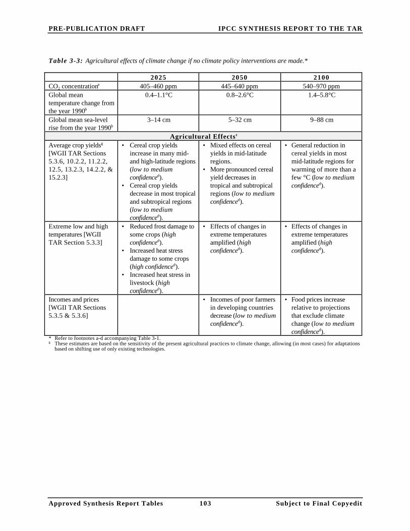
PRE-PUBLICATION DRAFT IPCC SYNTHESIS REPORT TO THE TAR
Approved Synthesis Report Tables 103 Subject to Final Copyedit
Table 3-3: Agricultural effects of climate change if no climate policy interventions are made.* 2025 2050 2100 CO2 concentrationa 405–460 ppm 445–640 ppm 540–970 ppm Global meantemperature change fromthe year 1990b
0.4–1.1°C 0.8–2.6°C 1.4–5.8°C
Global mean sea-levelrise from the year 1990b
3–14 cm 5–32 cm 9–88 cm
Agricultural Effectsc
Average crop yieldsg
[WGII TAR Sections5.3.6, 10.2.2, 11.2.2,12.5, 13.2.3, 14.2.2, &15.2.3]
• Cereal crop yieldsincrease in many mid-and high-latitude regions(low to mediumconfidenced).
• Cereal crop yieldsdecrease in most tropicaland subtropical regions(low to mediumconfidenced).
• Mixed effects on cerealyields in mid-latituderegions.
• More pronounced cerealyield decreases intropical and subtropicalregions (low to mediumconfidenced).
• General reduction incereal yields in mostmid-latitude regions forwarming of more than afew °C (low to mediumconfidenced).
Extreme low and hightemperatures [WGIITAR Section 5.3.3]
• Reduced frost damage tosome crops (highconfidenced).
• Increased heat stressdamage to some crops(high confidenced).
• Increased heat stress inlivestock (highconfidenced).
• Effects of changes inextreme temperaturesamplified (highconfidenced).
• Effects of changes inextreme temperaturesamplified (highconfidenced).
Incomes and prices[WGII TAR Sections5.3.5 & 5.3.6]
• Incomes of poor farmersin developing countriesdecrease (low to mediumconfidenced).
• Food prices increaserelative to projectionsthat exclude climatechange (low to mediumconfidenced).
* Refer to footnotes a-d accompanying Table 3-1. g These estimates are based on the sensitivity of the present agricultural practices to climate change, allowing (in most cases) for adaptations
based on shifting use of only existing technologies.

PRE-PUBLICATION DRAFT IPCC SYNTHESIS REPORT TO THE TAR
Approved Synthesis Report Tables 104 Subject to Final Copyedit
Table 3-4: Water resource effects of climate change if no climate policy interventions are made.* 2025 2050 2100 CO2 concentrationa 405–460 ppm 445–640 ppm 540–970 ppm Global meantemperature change fromthe year 1990b
0.4–1.1°C 0.8–2.6°C 1.4–5.8°C
Global mean sea-levelrise from the year 1990b
3–14 cm 5–32 cm 9–88 cm
Water Resource Effects Water supply [WGIITAR Sections 4.3.6 &4.5.2]
• Peak river flow shiftsfrom spring towardwinter in basins wheresnowfall is an importantsource of water (highconfidenced).
• Water supply decreasedin many water-stressedcountries, increased insome other water-stressed countries (highconfidenced).
• Water supply effectsamplified (highconfidenced).
Water quality [WGIITAR Section 4.3.10]
• Water quality degradedby higher temperatures.
• Water quality changesmodified by changes inwater flow volume.
• Increase in saltwaterintrusion into coastalaquifers due to sea-levelrise (mediumconfidenced).
• Water quality degradedby highertemperatures(highconfidenced).
• Water quality changesmodified by changes inwater flow volume (highconfidenced).
• Water quality effectsamplified (highconfidenced).
Water demand [WGIITAR Section 4.4.3]
• Water demand forirrigation will respondto changes in climate;higher temperatures willtend to increase demand(high confidenced).
• Water demand effectsamplified (highconfidenced).
• Water demand effectsamplified (highconfidenced).
Extreme events [WGITAR SPM; WGII TARSPM]
• Increased flood damagedue to more intenseprecipitation events(high confidenced).
• Increased droughtfrequency (highconfidenced).
• Further increase in flooddamage (highconfidenced).
• Further increase indrought events and theirimpacts.
• Flood damage several-fold higher than “noclimate changescenarios.”
* Refer to footnotes a-d accompanying Table 3-1.

PRE-PUBLICATION DRAFT IPCC SYNTHESIS REPORT TO THE TAR
Approved Synthesis Report Tables 105 Subject to Final Copyedit
Table 3-5: Other market sector effects of climate change if no climate policy interventions are made.*
2025 2050 2100CO2 concentrationa 405–460 ppm 445–640 ppm 540–970 ppmGlobal meantemperature change fromthe year 1990b
0.4–1.1°C 0.8–2.6°C 1.4–5.8°C
Global mean sea-levelrise from the year 1990b
3–14 cm 5–32 cm 9–88 cm
Other Market Sector Effectsc
Energy [WGII TARSection 7.3]
• Decreased energy demandfor heating buildings(high confidenced).
• Increased energy demandfor cooling buildings(high confidenced).
• Energy demand effectsamplified (highconfidenced).
• Energy demand effectsamplified (highconfidenced).
Financial sector [WGIITAR Section 8.3]
• Increased insuranceprices and reducedinsurance availability(high confidenced).
• Effects on financialsector amplified.
Aggregate marketeffectse [WGII TARSections 19.4-5]
• Net market sector lossesin many developingcountries (lowconfidenced).
• Mixture of market gainsand losses in developedcountries (lowconfidenced).
• Losses in developingcountries amplified(medium confidenced).
• Gains diminished andlosses amplified indeveloped countries(medium confidenced).
• Losses in developingcountries amplified(medium confidenced).
• Net market sector lossesin developed countriesform warming of morethan a few °C (mediumconfidenced).
* Refer to footnotes a-d accompanying Table 3-1 and footnote e accompanying Table 3-2.

PRE-PUBLICATION DRAFT IPCC SYNTHESIS REPORT TO THE TAR
Approved Synthesis Report Tables 106 Subject to Final Copyedit
Table 3-6: Examples of adaptation options for selected sectors.
Sector/System Adaptation OptionsWater [WGII TARSections 4.6 & 7.5.3;WGII SAR Sections10.6.4 & 14.4]
• Increase water-use efficiency with “demand-side” management (e.g., pricing incentives,regulations, technology standards).
• Increase water supply, or reliability of water supply, with “supply-side” management(e.g., construct new water storage and diversion infrastructure).
• Change institutional and legal framework to facilitate transfer of water among users (e.g.,establish water markets).
• Reduce nutrient loadings of rivers and protect/augment streamside vegetation to offseteutrophying effects of higher water temperatures.
• Reform flood management plans to reduce downstream flood peaks; reduce paved surfacesand use vegetation to reduce storm runoff and increase water infiltration.
• Reevaluate design criteria of dams, levees, and other infrastructure for flood protection. Food and fiber [WGIITAR Sections 5.3.4& 5.3.5; WGII SARSections 2.9, 4.4.4,13.9, & 15.6; SRTTSection 11.2.1]
• Change timing of planting, harvesting, and other management activities.• Use minimum tillage and other practices to improve nutrient and moisture retention in
soils and to prevent soil erosion.• Alter animal stocking rates on rangelands.• Switch to crops or crop cultivars that are less water demanding and more tolerant of heat,
drought, and pests.• Conduct research to develop new cultivars.• Promote agroforestry in dryland areas, including establishment of village woodlots and
use of shrubs and trees for fodder.• Replant with mix of tree species to increase diversity and flexibility. Promote
revegetation and reforestation initiatives.• Assist natural migration of tree species with connected protected areas and transplanting.• Improve training and education of rural work forces.• Establish or expand programs to provide secure food supplies as insurance against local
supply disruptions.• Reform policies that encourage inefficient, non-sustainable, or risky farming, grazing,
and forestry practices (e.g., subsidies for crops, crop insurance, water). Coastal areas andmarine fisheries[WGII TAR Sections6.6 & 7.5.3; WGIISAR Section 16.3;SRTT Section 15.4]
• Prevent or phase-out development in coastal areas vulnerable to erosion, inundation, andstorm-surge flooding.
• Use “hard” (dikes, levees, seawalls) or “soft” (beach nourishment, dune and wetlandrestoration, afforestation) structures to protect coasts.
• Implement storm warning systems and evacuation plans.• Protect and restore wetlands, estuaries, and floodplains to preserve essential habitat for
fisheries.• Modify and strengthen fisheries management institutions and policies to promote
conservation of fisheries.• Conduct research and monitoring to better support integrated management of fisheries.
Human health [WGII TAR Sections7.5.3 & 9.11; WGIISAR Section 12.5;SRTT Section 14.4]
• Rebuild and improve public health infrastructure.• Improve epidemic preparedness and develop capacities for epidemic forecasting and early
warning.• Monitor environmental, biological, and health status.• Improve housing, sanitation, and water quality.• Integrate urban designs to reduce heat island effect (e.g., use of vegetation and light
colored surfaces).• Conduct public education to promote behaviors that reduce health risks.
Financial services [WGII TAR Section8.3.4]
• Risk spreading through private and public insurance and reinsurance.• Risk reduction through building codes and other standards set or influenced by financial
sector as requirements for insurance or credit.
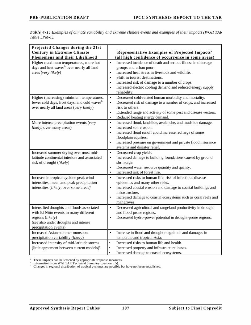
PRE-PUBLICATION DRAFT IPCC SYNTHESIS REPORT TO THE TAR
Approved Synthesis Report Tables 107 Subject to Final Copyedit
Table 4-1: Examples of climate variability and extreme climate events and examples of their impacts (WGII TARTable SPM-1).
Projected Changes during the 21stCentury in Extreme ClimatePhenomena and their Likelihood
Representative Examples of Projected Impactsa
(all high confidence of occurrence in some areas)Higher maximum temperatures, more hotdays and heat wavesb over nearly all landareas (very likely)
• Increased incidence of death and serious illness in older agegroups and urban poor.
• Increased heat stress in livestock and wildlife.• Shift in tourist destinations.• Increased risk of damage to a number of crops.• Increased electric cooling demand and reduced energy supply
reliability.Higher (increasing) minimum temperatures,fewer cold days, frost days, and cold wavesb
over nearly all land areas (very likely)
• Decreased cold-related human morbidity and mortality.• Decreased risk of damage to a number of crops, and increased
risk to others.• Extended range and activity of some pest and disease vectors.• Reduced heating energy demand.
More intense precipitation events (verylikely, over many areas)
• Increased flood, landslide, avalanche, and mudslide damage.• Increased soil erosion.• Increased flood runoff could increase recharge of some
floodplain aquifers.• Increased pressure on government and private flood insurance
systems and disaster relief.Increased summer drying over most mid-latitude continental interiors and associatedrisk of drought (likely)
• Decreased crop yields.• Increased damage to building foundations caused by ground
shrinkage.• Decreased water resource quantity and quality.• Increased risk of forest fire.
Increase in tropical cyclone peak windintensities, mean and peak precipitationintensities (likely, over some areas)c
• Increased risks to human life, risk of infectious diseaseepidemics and many other risks.
• Increased coastal erosion and damage to coastal buildings andinfrastructure.
• Increased damage to coastal ecosystems such as coral reefs andmangroves.
Intensified droughts and floods associatedwith El Niño events in many differentregions (likely)(see also under droughts and intenseprecipitation events)
• Decreased agricultural and rangeland productivity in drought-and flood-prone regions.
• Decreased hydro-power potential in drought-prone regions.
Increased Asian summer monsoonprecipitation variability (likely)
• Increase in flood and drought magnitude and damages intemperate and tropical Asia.
Increased intensity of mid-latitude storms(little agreement between current models)b
• Increased risks to human life and health.• Increased property and infrastructure losses.• Increased damage to coastal ecosystems.
a These impacts can be lessened by appropriate response measures.b Information from WGI TAR Technical Summary (Section F.5).c Changes in regional distribution of tropical cyclones are possible but have not been established.
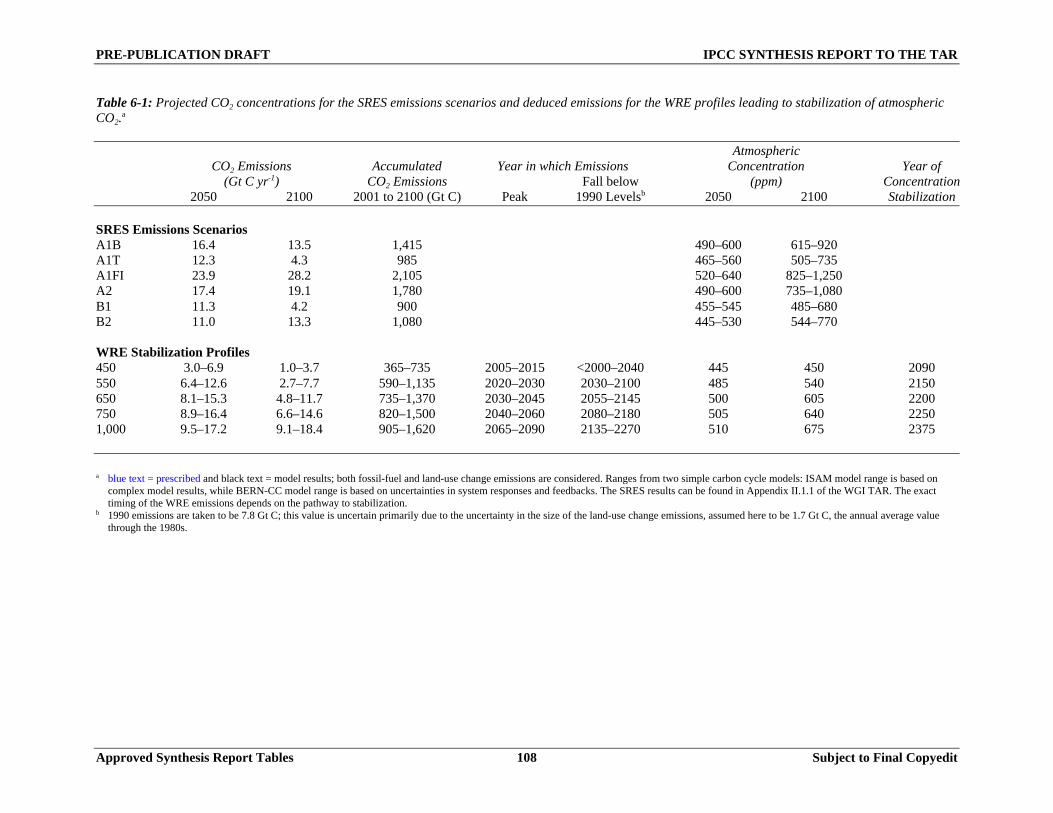
PRE-PUBLICATION DRAFT IPCC SYNTHESIS REPORT TO THE TAR
Approved Synthesis Report Tables 108 Subject to Final Copyedit
Table 6-1: Projected CO2 concentrations for the SRES emissions scenarios and deduced emissions for the WRE profiles leading to stabilization of atmosphericCO2.
a
AtmosphericCO2 Emissions Accumulated Year in which Emissions Concentration Year of
(Gt C yr-1) CO2 Emissions Fall below (ppm) Concentration2050 2100 2001 to 2100 (Gt C) Peak 1990 Levelsb 2050 2100 Stabilization
SRES Emissions ScenariosA1B 16.4 13.5 1,415 490–600 615–920A1T 12.3 4.3 985 465–560 505–735A1FI 23.9 28.2 2,105 520–640 825–1,250A2 17.4 19.1 1,780 490–600 735–1,080B1 11.3 4.2 900 455–545 485–680B2 11.0 13.3 1,080 445–530 544–770
WRE Stabilization Profiles450 3.0–6.9 1.0–3.7 365–735 2005–2015 <2000–2040 445 450 2090550 6.4–12.6 2.7–7.7 590–1,135 2020–2030 2030–2100 485 540 2150650 8.1–15.3 4.8–11.7 735–1,370 2030–2045 2055–2145 500 605 2200750 8.9–16.4 6.6–14.6 820–1,500 2040–2060 2080–2180 505 640 22501,000 9.5–17.2 9.1–18.4 905–1,620 2065–2090 2135–2270 510 675 2375
a blue text = prescribed and black text = model results; both fossil-fuel and land-use change emissions are considered. Ranges from two simple carbon cycle models: ISAM model range is based oncomplex model results, while BERN-CC model range is based on uncertainties in system responses and feedbacks. The SRES results can be found in Appendix II.1.1 of the WGI TAR. The exacttiming of the WRE emissions depends on the pathway to stabilization.
b 1990 emissions are taken to be 7.8 Gt C; this value is uncertain primarily due to the uncertainty in the size of the land-use change emissions, assumed here to be 1.7 Gt C, the annual average valuethrough the 1980s.
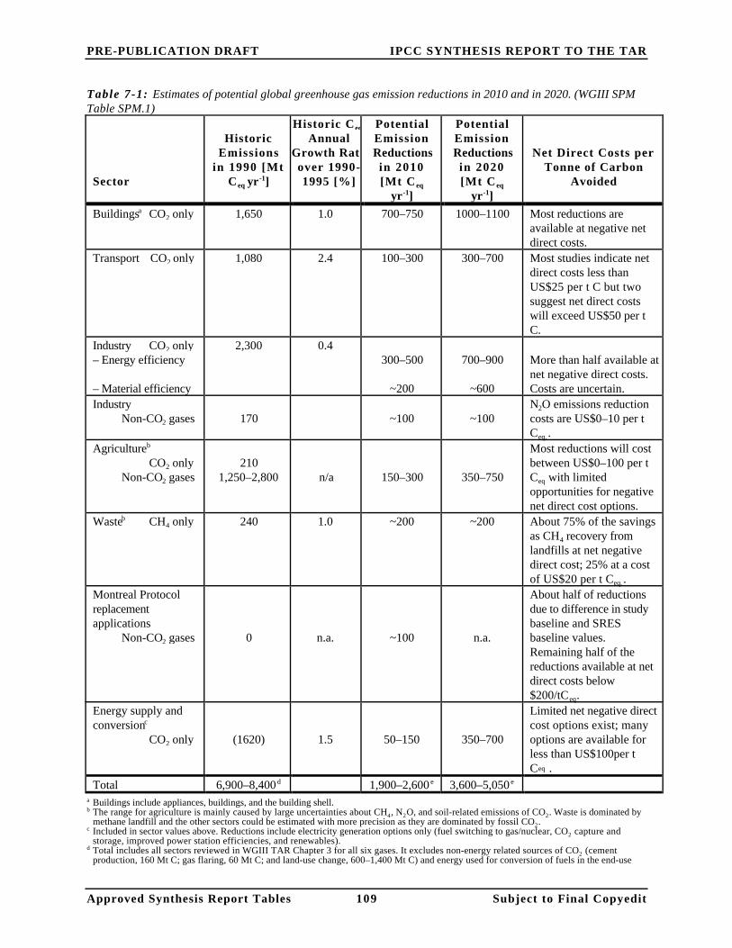
PRE-PUBLICATION DRAFT IPCC SYNTHESIS REPORT TO THE TAR
Approved Synthesis Report Tables 109 Subject to Final Copyedit
Table 7-1: Estimates of potential global greenhouse gas emission reductions in 2010 and in 2020. (WGIII SPMTable SPM.1)
Sector
HistoricEmissions
in 1990 [MtCeq yr-1]
Historic Ceq.
AnnualGrowth Rateover 1990-1995 [%]
PotentialEmissionReductionsin 2010[Mt C eq
yr-1]
PotentialEmissionReductionsin 2020[Mt C eq
yr-1]
Net Direct Costs perTonne of Carbon
Avoided
Buildingsa CO2 only 1,650 1.0 700–750 1000–1100 Most reductions areavailable at negative netdirect costs.
Transport CO2 only 1,080 2.4 100–300 300–700 Most studies indicate netdirect costs less thanUS$25 per t C but twosuggest net direct costswill exceed US$50 per tC.
Industry CO2 only– Energy efficiency
– Material efficiency
2,300 0.4300–500
~200
700–900
~600
More than half available atnet negative direct costs.Costs are uncertain.
IndustryNon-CO2 gases 170 ~100 ~100
N2O emissions reductioncosts are US$0–10 per tCeq. .
Agricultureb
CO2 onlyNon-CO2 gases
2101,250–2,800 n/a 150–300 350–750
Most reductions will costbetween US$0–100 per tCeq with limitedopportunities for negativenet direct cost options.
Wasteb CH4 only 240 1.0 ~200 ~200 About 75% of the savingsas CH4 recovery fromlandfills at net negativedirect cost; 25% at a costof US$20 per t Ceq. .
Montreal Protocolreplacementapplications
Non-CO2 gases 0 n.a. ~100 n.a.
About half of reductionsdue to difference in studybaseline and SRESbaseline values.Remaining half of thereductions available at netdirect costs below$200/tCeq.
Energy supply andconversionc
CO2 only (1620) 1.5 50–150 350–700
Limited net negative directcost options exist; manyoptions are available forless than US$100per tCeq..
Total 6,900–8,400 d 1,900–2,600 e 3,600–5,050 e
a Buildings include appliances, buildings, and the building shell.b The range for agriculture is mainly caused by large uncertainties about CH4, N2O, and soil-related emissions of CO2. Waste is dominated by
methane landfill and the other sectors could be estimated with more precision as they are dominated by fossil CO2.c Included in sector values above. Reductions include electricity generation options only (fuel switching to gas/nuclear, CO2 capture and
storage, improved power station efficiencies, and renewables).d Total includes all sectors reviewed in WGIII TAR Chapter 3 for all six gases. It excludes non-energy related sources of CO2 (cement
production, 160 Mt C; gas flaring, 60 Mt C; and land-use change, 600–1,400 Mt C) and energy used for conversion of fuels in the end-use

PRE-PUBLICATION DRAFT IPCC SYNTHESIS REPORT TO THE TAR
Approved Synthesis Report Tables 110 Subject to Final Copyedit
sector totals (630 Mt C). If petroleum refining and coke oven gas were added, global year 1990 CO2 emissions of 7,100 Mt C would increaseby 12%. Note that forestry emissions and their carbon sink mitigation options are not included.
e The baseline SRES scenarios (for six gases included in the Kyoto Protocol) project a range of emissions of 11,500–14,000 Mt Ceq for the year2010 and of 12,000–16,000 Mt Ceq for the year 2020. The emissions reduction estimates are most compatible with baseline emissions trends inthe SRES B2 scenario. The potential reductions take into account regular turnover of capital stock. They are not limited to cost-effectiveoptions, but exclude options with costs above US$100 t Ceq (except for Montreal Protocol gases) or options that will not be adopted throughthe use of generally accepted policies.
Table 7-2: Estimates of potential global greenhouse gas emission reductions in the year 2010: land use, land-usechange, and forestry.
Categories ofMitigation Options
PotentialEmission
Reductionsin 2010
[Mt C yr -1]
PotentialEmission
Reductions[Mt C]
Afforestation/reforestation (AR)a 197–584 Includes carbon in above- and below-ground biomass. Excludes carbon in soilsand in dead organic matter.
Reducing deforestation (D)b 1,788 Potential for reducing deforestation isvery uncertain for the tropics and could bein error by as much as ±50%.
Improved management within aland use (IM)c
570 Assumed to be the best available suite ofmanagement practices for each land useand climatic zone.
Land-use change (LC)c 435
Total 1,202–1,589 1,788
a Source: SRLULUCF Table SPM-3. Based on IPCC definitional scenario. Information is not available for other definitional scenarios. Potentialrefers to the estimated range of accounted average stock change for the period 2008–2012 (Mt C yr-1 ).
b Source: SRLULUCF Table SPM-3. Based on IPCC definitional scenario. Information is not available for other definitional scenarios.Potential refers to the estimated average stock change (Mt C).
c Source: SRLULUCF Table SPM-4. Potential refers to the estimated net change in carbon stocks in the year 2010 (Mt C yr-1 ). The list ofactivities is not exclusive or complete, and it is unlikely that all countries will apply all activities. Some of these estimates reflect considerableuncertainty.

PRE-PUBLICATION DRAFT IPCC SYNTHESIS REPORT TO THE TAR
Approved Synthesis Report Tables 111 Subject to Final Copyedit
Table 7-3: Results of model comparison from the Energy Modeling Forum.a
(a) Calculated losses (as % of total GDP) for various postulated trading regimes associated with meeting the Kyototargets in Annex-B countries
No Trading Annex I Trading
Model CANZ USAOECDEurope Japan CANZ USA
OECDEurope Japan
ABARE-GTEM 1.96 1.96 0.94 0.72 0.23 0.47 0.13 0.05AIM 0.59 0.45 0.31 0.25 0.36 0.31 0.17 0.13CETA 1.93 0.67G-Cubed 1.83 0.42 1.50 0.57 0.72 0.24 0.61 0.45GRAPE 0.81 0.19 0.81 0.10MERGE3 2.02 1.06 0.99 0.80 1.14 0.51 0.47 0.19MS-MRT 1.83 1.88 0.63 1.20 0.88 0.91 0.13 0.22RICE 0.96 0.94 0.55 0.78 0.54 0.56 0.28 0.30
(b) Marginal abatement costs (in 1990 US$ per t C; 2010 Kyoto target)
Model CANZ USAOECDEurope Japan
Annex I Trading
ABARE-GTEM 425 322 665 645 106
AIM 147 153 198 234 65
CETA 168 46
G-Cubed 157 76 227 97 53
GRAPE 204 304 70
MERGE3 250 264 218 500 135
MS-MRT 213 236 179 402 77
RICE 145 132 159 251 62
SGM 201 188 407 357 84
(c) Costs of Kyoto Protocol implementation for oil-exporting countries according to various modelsb
Modelc Without Trading dWith Annex I
TradingWith “Global
Trading”G-Cubed -25% oil revenue -13% oil revenue -7% oil revenueGREEN -3% real income “substantially reduced
loss”n/a
GTEM 0.2% GDP loss <0.05% GDP loss n/aMS-MRT 1.39% welfare loss 1.15% welfare loss 0.36% welfare loss
OPEC -17% OPEC Revenue -10% OPEC revenue -8% OPEC revenueCLIMOX n/a -10% some oil
exporters’ revenuesn/a
a Table 7-3a derived from WGIII TAR Table TS.5, Table 7-3b from WGIII TAR Table TS.4, and Table 7-3c from WGIII TAR Table TS.6.b The definition of oil-exporting country varies. For G-Cubed and the OPEC models, it is the OPEC countries; for GREEN, a group of oil-
exporting countries; for GTEM, Mexico and Indonesia; for MS-MRT, OPEC countries plus Mexico; and for CLIMOX, west Asian andnorth African oil exporters.
c The models are all considering the global economy to the year 2010 with mitigation according to the Kyoto Protocol targets (usually in themodels applied to CO2 mitigation by the year 2010 rather than greenhouse gas emissions to the period 2008-2012) achieved by imposing acarbon tax or auctioned emission permits with revenues recycled through lump-sum payments to consumers. No co-benefits, such asreductions in local air pollution damages, are taken into account in the results.
d “Trading” denotes trading in emission permits between countries.n/a = not available

PRE-PUBLICATION DRAFT IPCC SYNTHESIS REPORT TO THE TAR
Approved Synthesis Report Tables 112 Subject to Final Copyedit
Table 8-1: Examples for observed and projected regional implications of climate change on natural ecosystems,biodiversity, and food supply.
Region ImpactsReferenceSection inWGII TAR
Africa • Irreversible losses of biodiversity could be accelerated with climatechange.
• Significant extinctions of plant and animal species are projectedand would impact rural livelihoods, tourism, and genetic resources(medium confidence).
TS 5.1.3 &Section 10.2.3.2
Asia • Decreases in agricultural productivity and aquaculture due tothermal and water stress, sea-level rise, floods and droughts, andtropical cyclones would diminish food security in many countriesof arid, tropical, and temperate Asia; agriculture would expand andincrease in productivity in northern areas (medium confidence).
• Climate change would exacerbate threat to biodiversity due to land-use and land-cover change and population pressure (mediumconfidence). Sea-level rise would put ecological security at riskincluding mangroves and coral reefs (high confidence).
TS 5.2.1-2 &Sections 11.2.1-2
Australia and NewZealand
• A warming of 1ºC would threaten the survival of species currentlynear the upper limit of their temperature range, notably in marginalalpine regions.
• Some species with restricted climatic niches and that are unable tomigrate due to fragmentation of the landscape soil differences ortopography could become endangered or extinct (high confidence).Australian ecosystems that are particularly vulnerable to climatechange include coral reefs, arid and semi-arid habitats in southwestand inland Australia, and Australian alpine systems. Freshwaterwetlands in coastal zones in both Australia and New Zealand arevulnerable, and some New Zealand ecosystems are vulnerable toaccelerated invasion by weeds.
TS 5.3.2 &Sections 12.4.2,12.4.4-5, & 12.4.7
Europe • Natural ecosystems will change due to increasing temperature andatmospheric concentration of CO2. Diversity in nature reserves isunder threat of rapid change. Loss of important habitats (wetlands,tundra, and isolated habitats) would threaten some species,including rare/endemic species and migratory birds.
• There will be some broadly positive effects on agriculture innorthern Europe (medium confidence); productivity will decrease insouthern and eastern Europe (medium confidence).
TS 5.4.2-3 &Sections 13.2.1.4,13.2.2.1, 13.2.2.3-5, & 13.2.3.1

PRE-PUBLICATION DRAFT IPCC SYNTHESIS REPORT TO THE TAR
Approved Synthesis Report Tables 113 Subject to Final Copyedit
Table 8-1 (continued)
Region ImpactsReferenceSection inWGII TAR
Latin America • It is well-established that Latin America accounts for one of theEarth’s largest concentrations of biodiversity and the impacts ofclimate change can be expected to increase the risk of biodiversityloss (high confidence).
• Yields of important crops are projected to decrease in manylocations even when the effects of CO2 are taken into account;subsistence farming in some regions could be threatened (highconfidence).
TS 5.5.2 & 5.5.4,& Sections 14.2.1-2
North America • There is strong evidence that climate change can lead to the loss ofspecific ecosystem types (e.g., high alpine areas and specificcoastal (salt marshes and inland prairie “potholes”) wetlands) (highconfidence).
• Some crops would benefit from modest warming accompanied byincreasing CO2, but effect would vary among crops and regions(high confidence), including declines due to drought in some areasof Canada’s Prairies and the U.S. Great Plains, potential increasedfood production in areas of Canada north of current productionareas, and increased warm temperate mixed forest production(medium confidence). However, benefits for crops would decline atan increasing rate and possibly become a net loss with furtherwarming (medium confidence).
• Unique natural ecosystems such as prairie wetlands, alpine tundra,and coldwater ecosystems will be at risk and effective adaptation isunlikely (medium confidence).
TS 5.6.4-5 &Sections 15.2.2-3
Arctic • The Arctic is extremely vulnerable to climate change, and majorphysical, ecological, and economic impacts are expected to appearrapidly.
TS 5.7 & Sections16.2.7-8
Antarctic • In the Antarctic projected climate change will generate impacts thatwill be realized slowly (high confidence).
• Warmer temperatures and reduced ice extent are likely to producelong-term changes in the physical oceanography and ecology of theSouthern Ocean, with intensified biological activity and increasedgrowth rate of fish.
TS 5.7 & Sections16.2.3 & 16.2.4.2
Small Islands • Projected future climate change and sea-level rise will affect shiftsin species composition and competition. It is estimated that oneout of every three (30%) known threatened plants are islandsendemics, while 23% of bird species are threatened. Coral reefs,mangroves, and seagrass beds that often rely on stableenvironmental conditions will be adversely affected by rising airand sea temperatures and sea-level rise (medium confidence).
• Declines in coastal ecosystems would negatively impact reef fishand threaten reef fisheries (medium confidence).
TS 5.8 & Sections17.2.4-5 &17.2.8.2

PRE-PUBLICATION DRAFT IPCC SYNTHESIS REPORT TO THE TAR
Approved Synthesis Report Tables 114 Subject to Final Copyedit
Table 8-2: Examples of regional impacts of climate change on water resources, land degradation, anddesertification.
R e g i o n Projec t ionsReferenceSec t ion inWGII TAR
Africa • Changes in rainfall and intensified land use would exacerbate thedesertification processes. Desertification would be exacerbated byreduction in the average annual rainfall, runoff, and soil moisture incountries of west African Sahel, and northern and southern Africa(medium confidence). Increases in droughts and other extreme eventswould add to stresses on water resources, food security, and humanhealth, and would constrain development in the region (highconfidence).
TS 5.1.6, Chapter10 ES, Sections10.2.1 & 10.2.6, &Table SPM-2
Asia • Water shortage—already a limiting factor for ecosystems, food andfiber production, human settlements, and human health—may beexacerbated by climate change. Runoff and water availability maydecrease in arid and semi-arid Asia but increase in northern Asia(medium confidence). Reduced soil moisture in summer wouldexacerbate land degradation and desertification in arid and semi-aridregions.
TS 5.2.3 & Sections11.1.1 & 11.2.3
Australia and NewZealand
• Interannual variability due to ENSO leads to major floods and droughtsin Australia and New Zealand. Such variations are expected to continueunder enhanced greenhouse gas conditions, but possibly with greaterhydrological extremes.
• Water is likely to be a key issue (high confidence) due to projecteddrying trends over much of the region and change to a more El Niño-like event state. Water quality would be affected, and more intenserainfall events would increase fast runoff, soil erosion, and sedimentloading. Eutrophication is a major water quality problem in Australia.
TS 5.3 & Sections12.1.5.3 & 12.3
Europe • Summer runoff, water availability, and soil moisture are likely todecrease in southern Europe, and would widen the gap between thenorth and south (high confidence). Flood hazards will increase acrossmuch of Europe (medium to high confidence); risk would be substantialfor coastal areas where flooding will increase erosion and result in lossof wetlands.
• Half of alpine glaciers and large permafrost areas could disappear bythe end of the 21st century (medium confidence).
TS 5.4.1, Chapter13 ES, & Section13.2.1
Latin America • Some studies based on model experiments suggest that under climatechange the hydrological cycle would be more intense, with changes inthe distribution of extreme rainfall, wet spells, and dry spells. Frequentsevere drought in Mexico during the last decade coincides with some ofthese model findings. El Niño is related to dry conditions innortheastern Brazil, northern Amazons, and the Peruvian-Bolivianaltiplano. Southern Brazil and northwestern Peru exhibit anomalouswet conditions during these periods.
• Loss and retreat of glaciers would adversely impact runoff and watersupply in areas where snowmelt is an important water resource (highconfidence).
TS 5.5.1, Chapter14 ES, & Section14.2.4
North America • Snowmelt-dominated watersheds in western North America willexperience earlier spring peak flows (high confidence) and reductionin summer flow (medium confidence); adaptive responses may offsetsome, but not all, of the impacts on water resources and aquaticecosystems (medium confidence).
TS 5.6.2, Section15.2.1, & TableSPM-2
Small Islands • Islands with very limited water supplies are highly vulnerable to theimpacts of climate change on the water balance (high confidence).
TS 5.8.4, Section17.2.6, & TableSPM-2
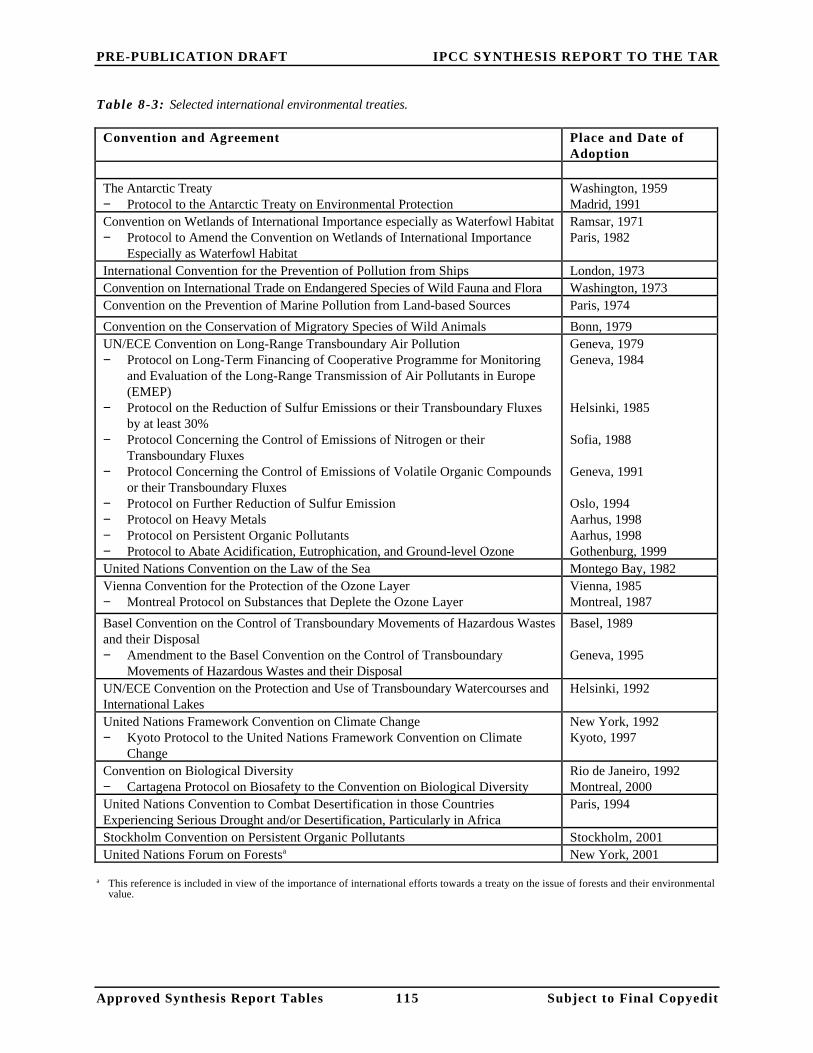
PRE-PUBLICATION DRAFT IPCC SYNTHESIS REPORT TO THE TAR
Approved Synthesis Report Tables 115 Subject to Final Copyedit
Table 8-3: Selected international environmental treaties.
Convention and Agreement Place and Date ofAdoption
The Antarctic Treaty− Protocol to the Antarctic Treaty on Environmental Protection
Washington, 1959Madrid, 1991
Convention on Wetlands of International Importance especially as Waterfowl Habitat− Protocol to Amend the Convention on Wetlands of International Importance
Especially as Waterfowl Habitat
Ramsar, 1971Paris, 1982
International Convention for the Prevention of Pollution from Ships London, 1973Convention on International Trade on Endangered Species of Wild Fauna and Flora Washington, 1973Convention on the Prevention of Marine Pollution from Land-based Sources Paris, 1974
Convention on the Conservation of Migratory Species of Wild Animals Bonn, 1979UN/ECE Convention on Long-Range Transboundary Air Pollution− Protocol on Long-Term Financing of Cooperative Programme for Monitoring
and Evaluation of the Long-Range Transmission of Air Pollutants in Europe(EMEP)
− Protocol on the Reduction of Sulfur Emissions or their Transboundary Fluxesby at least 30%
− Protocol Concerning the Control of Emissions of Nitrogen or theirTransboundary Fluxes
− Protocol Concerning the Control of Emissions of Volatile Organic Compoundsor their Transboundary Fluxes
− Protocol on Further Reduction of Sulfur Emission− Protocol on Heavy Metals− Protocol on Persistent Organic Pollutants− Protocol to Abate Acidification, Eutrophication, and Ground-level Ozone
Geneva, 1979Geneva, 1984
Helsinki, 1985
Sofia, 1988
Geneva, 1991
Oslo, 1994Aarhus, 1998Aarhus, 1998Gothenburg, 1999
United Nations Convention on the Law of the Sea Montego Bay, 1982Vienna Convention for the Protection of the Ozone Layer− Montreal Protocol on Substances that Deplete the Ozone Layer
Vienna, 1985Montreal, 1987
Basel Convention on the Control of Transboundary Movements of Hazardous Wastesand their Disposal− Amendment to the Basel Convention on the Control of Transboundary
Movements of Hazardous Wastes and their Disposal
Basel, 1989
Geneva, 1995
UN/ECE Convention on the Protection and Use of Transboundary Watercourses andInternational Lakes
Helsinki, 1992
United Nations Framework Convention on Climate Change− Kyoto Protocol to the United Nations Framework Convention on Climate
Change
New York, 1992Kyoto, 1997
Convention on Biological Diversity− Cartagena Protocol on Biosafety to the Convention on Biological Diversity
Rio de Janeiro, 1992Montreal, 2000
United Nations Convention to Combat Desertification in those CountriesExperiencing Serious Drought and/or Desertification, Particularly in Africa
Paris, 1994
Stockholm Convention on Persistent Organic Pollutants Stockholm, 2001United Nations Forum on Forestsa New York, 2001
a This reference is included in view of the importance of international efforts towards a treaty on the issue of forests and their environmentalvalue.

116
PRE-PUBLICATION DRAFT IPCC SYNTHESIS REPORT TO THE TAR
Approved Synthesis Report Illustrations Subject to Final Copyedit
��������������������� ������ ����� �
����������������������������
��������� ������������������������ ���
���������������� �����
������������ ������������������� ����������
������������ � ���� ���������������� ������ ����
!��������������!��������
� ������������"� �����
����� ��� �� ������������� ���
� ���������������# ���������������
"��������$��������
"��������
Figure 1-1

117
PRE-PUBLICATION DRAFT IPCC SYNTHESIS REPORT TO THE TAR
Approved Synthesis Report Illustrations Subject to Final Copyedit
�
��
��
���
���
���
���
���
���
%����������� ����&'��()
���� ���� ���� ���� ���� ����
�� ��#��*���
��
��
��
��
�+(����
���
�����
�����
�����
�����
�!,����
$����
���
���
���
%����������� ����&'��()
���� ���� ���� ���� ���� ����
-�� ����+*���
-(+����
���
���
���
���
���
���
���
���
���� ���� ���� ���� ���� ����
%����������� ����&'��()
�����
���� ���� �����
���
���
������������� ����������
������������������
�+(����������������������� ��!
���"#����$����%� &�
������� ������������������������������� ���� ����������� ����� �
��� ���������� �������� ��������� ����������*���� ������������
���������� ������������������� ���������
����
Figure 2-1
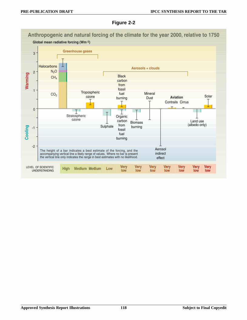
118
PRE-PUBLICATION DRAFT IPCC SYNTHESIS REPORT TO THE TAR
Approved Synthesis Report Illustrations Subject to Final Copyedit
&�
&�
�
�
�
�
��� ������� ����������� ����&'��()
"� �������������� ����� �������������������� ������� �(.../� �����������012.
'��
(��
� ������������
��� ��!�)�����*���
+)�� )���)�� ��� � � �� ����� ��!� � ��!�� �!��� ��� ��� �)�� �������,� ��� �)� ����� �%����-����� .�.���� �.�/�.%�� �������- .#�!��0)�������� ���!����!����)��-����� .�.������.%������ ��!��)��� ���������!���!��� ��!�1��)����.�/�.�)���
(2�
������
2 .�� ����!
+����!�)�����*���
�#.�) ��
��� ����� ����������!!�.�#�.
�#�����
3. �/�� ����������!!�.�#�.
�#�����
3��� !!�#�����
$���� .4#!�
5���!�.��������������
(���� �.! (���#!"������
"� ������3�������
6"7"6���8��(9"'+989(�'4":�+5'49';
'� ���
6 ���#!� .�������.%
��. �
Figure 2-2

119
PRE-PUBLICATION DRAFT IPCC SYNTHESIS REPORT TO THE TAR
Approved Synthesis Report Illustrations Subject to Final Copyedit
4� ��������������� �5���� ���������� ��� ���� 666
���� ���� ���� ���� ���� ���� ����
���� ���� ���� ���� ���� ����
��
��
&��
&��
��
��
��
����&��
&��
��
��
��
��������0,.���� ��&��� ��)
4������������ �#��!
#��� �� ���������� ��� ����7��&� ������0890�088.���� ���)
��������0...���� ��&-� �� �!������ �)
#��� �� ���������� ��� ����7��&� ������0890�088.���� ���)
4������������ �#��!
<��=%�� �
��
����
��
&��
&��
&��
&��
Figure 2-3

120
PRE-PUBLICATION DRAFT IPCC SYNTHESIS REPORT TO THE TAR
Approved Synthesis Report Illustrations Subject to Final Copyedit
����� ��� �������������7� ����� ��� �������������7�
&�)�-��� ����� ������� & )�"� ���������� �������
&��
&��
��
��
��
���� ���� ���� ����
$���.���!#.�!
��!��- ����!
���� ���� ���� ����&��
&��
��
��
��
$���.���!#.�!
��!��- ����!
����� ���� ������������������ �� ��������������� ��� �� ��������������� �0:9.
&��
&��
��
��
��
&��
&��
��
��
��
����� ��� �������������7�
&�)�-��� ���3�"� ���������� ���
&��
&��
��
��
��
$���.���!#.�!
��!��- ����!&��
&��
��
��
��
���� ���� ���� ����
Figure 2-4

121
PRE-PUBLICATION DRAFT IPCC SYNTHESIS REPORT TO THE TAR
Approved Synthesis Report Illustrations Subject to Final Copyedit
�
>����
>����
&����
&����
$�������� � "���� ���
�����;����
< ���
�������� ���� ����
%��������������������� ���������=..���� �
���� ���� ����
�������� ���� �������� ���� ����
�
>����
>����
&����
&����
�
>����
>����
&����
&����
$�������� �
$�������� �
Figure 2-5

122
PRE-PUBLICATION DRAFT IPCC SYNTHESIS REPORT TO THE TAR
Approved Synthesis Report Illustrations Subject to Final Copyedit
� >���? >���? >���? >���? >���?
� �������� ��������� ����� �
&���?&���?&���?&���?&���?
�"����� ������������ ���>�08..����0888
"��������� ��� ��� ���>��0819����0888
&�� &��� &��� &��� &��� � >��� >��� >��� >��� >��
� ������7���� �������
Figure 2-6a
Figure 2-6b

123
PRE-PUBLICATION DRAFT IPCC SYNTHESIS REPORT TO THE TAR
Approved Synthesis Report Illustrations Subject to Final Copyedit
09 (8 ,, 1(0=
�
��
��
��
��
��
��
��
����
"����������/�����������������?6�6������ �
���� ������������ ����
��� �������������*� ��������� �������&����������;�����)
+�� .����������.�!!�!
9�!#����.�!!�!
'#���������-���!
4�� � .� -�� ��
0=
Figure 2-7

124
PRE-PUBLICATION DRAFT IPCC SYNTHESIS REPORT TO THE TAR
Approved Synthesis Report Illustrations Subject to Final Copyedit
5�35�+
5�89
5�3�
3�
9���
���� ���
��
��
& )��+(����������&����)
���
���
����
&�)��!,����������&����!,)
��
��
��
&�)�-(+����������&���-)
��
���
���
&�)��+(����������&����)
&�)��+(������ �����&���)
&�)��!,������ �����&�� )
&)�-(+������ �����&�� )
&�)����������� �����&����)
���
���
���
���
����
���
��
��
��
��
���
���
����
����&�)
����������������� ��� �������� ����� �����
$� ���� ��
$� � ������
$� ��������
$� ���� ������
"0��<�������
>�� . ����>���!!�.&�����!�-�>����&��!!�.
"(
<(<0
��
+)��5��!���%.���� ���!��� ����� ��.%���!�����! ��#�#���1��.�����-��%�� ����������������1�),�.�� .����#. ������) ���� /!�������&����#�%� �����.���!��)��� ����,� ����)��� ����������#����������1� ���������������������)��.����!�$ @��#����.%�����)���!� ������-�������� ����������!,�� � ���%&�#�.����,� �������� !���# . � # � . � �� �!�� � . �� � � � � � � � ��! , �1 � � ) �
!#�!� ��� .����#��������������� .�����������!�������� ��� ��������+)��5��!��� ����� ��.%��-�.��!�������)�������#�!��) � ���!�� ��� .���� ��-�����������!�������)��.���� .��) �������)�������%�!%!����+)���)����5�����#�!� ����!����#�!)����%��)�������)��.���� .����) !�!A��!!� . ������!�-��5�89 , ����&��!!� . ������%!�# � ��! �5�+ , �� � � �� . ��� � � ��!! � . .
!�#���!�5�3 �1)����� . ������!��������� !��� ��� .% ��������)� - � .% ��������� � � ��# . ������%�!�#���,�����)�� !!#��������) ��!���. ������-������ ��!� ��.%���� ..������%�!#��.% �������#!�����)��.����!
���� ���� ����
���� ���� ����
���� ���� ����
���� ���� ����
���� ���� ����
���� ���� ����
���� ���� ����
���� ���� ����
�����������������������
�������������������� �����
�����������
���������������
��� ����������
�����������������������
�������������������� �����
�����������������������
�������������������� �����
�����������
���������������
��� ���������������������
���������������
��� ����������
"0��/�"0�/����"0<
Figure 3-1
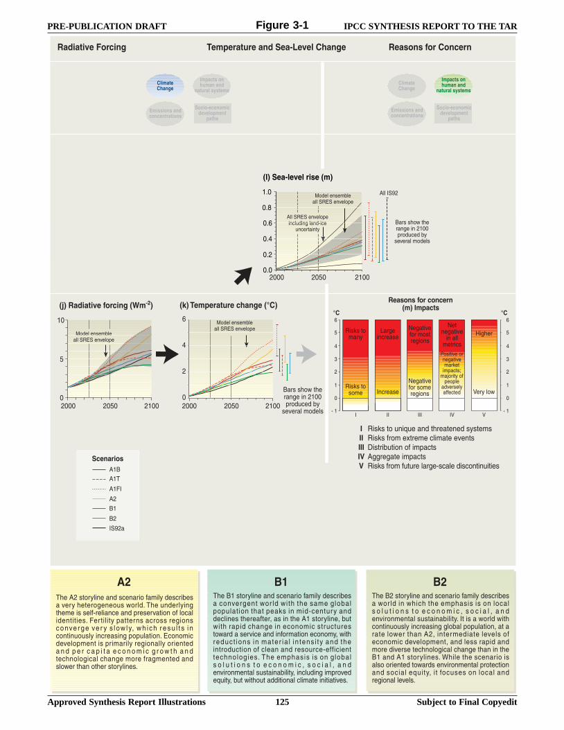
125
PRE-PUBLICATION DRAFT IPCC SYNTHESIS REPORT TO THE TAR
Approved Synthesis Report Illustrations Subject to Final Copyedit
:�!/!���� �%
6 �������� !�
'�� ��-�������!�������!
'����� ��-���� ..
������!
2��)��
:�!/!���!��� 9���� !�
'�� ��-�����!���������! 7��%�.�1
9 99 999 97 7
�
�
�
�
�
�
�
&��
7�
�
�
�
�
�
�
�
&��
7�
5�35�+
5�89
5�3�
3�
9���
���� ���
<�!���-������� ��-�� �/����� ��!B� @����%�������.�
�-��!�.% �������
%����������� ���
�
�
�
�
&�)������ ��� �������&7�)
��
��
��
��
��
��
&�)����������� ����&�)
&;)�%����������� ����&'��() &�)��������
���� ���������
�
��
3 �!�!)�1��)�� ���������������#�����%
!�-�� .�����.!
3 �!�!)�1��)�� ���������������#�����%
!�-�� .�����.!���� ��������
���� ��������
����� ��� ���������@��������� %�������� �����
5..�9���$���.���!���.� ..��:"����-�.���
$���.���!���.� ..��:"����-�.���
$���.���!���.� ..��:"����-�.���
+)��5��!���%.���� ���!��� ����� ��.%���!�����! �-��%�)����������#!�1��.��+)��#����.%����)�����!�!�.�&��.� ���� ������!��- ��������.�� .���������!�8����.��%�� �����!� ���!!�������!���-� ��� �-� � % �! . �1 . %, �1) � �) ���!# . � ! �� �������#�#!.%������ !�������#. �����"���������-�.��������!����� ��.%������� ..%��������� � � �� � � �� � � � �� � � � �� � � �� � �1 � ) � � ����)��.���� .��) ����������� �������� ��!.�1����) ����)���!���%.���!
+)��3��!���%.���� ���!��� ����� ��.%���!�����! ����-�������1�� .��1� �)��)��! ����.�� .���#. ������) ���� /!�������&����#�%� �����.���!��)��� ����,� !�����)��5��!���%.���,��#�1��)�� �����) ����������������!��#��#��!��1 ��� �!��-���� ��������� �����������%,�1��)���#�� ���!��� �� ��� � . ��� ���! � �% � ����)�������#����������.� �� �����!�#���&������������)��.����!�+)�����) !�!��! �����.�� .! � . # � � � � ! �� � �� � � � � � � � , �! � � � . , � � ���-�������� .�!#!� �� ��.��%,����.#����������-���C#��%,��#��1��)�#�� ������� .��.�� �������� ��-�!
+)��3��!���%.���� ���!��� ����� ��.%���!�����! �1�� .�����1)��)��)�����) !�!��!����.�� .! � . # � � � � ! �� � �� � � � �� � � , �! � � � . , � � ���-�������� .�!#!� �� ��.��%�9���!� �1��.��1��)������#�#!.%������ !�����.�� .����#. ����,� �� � ���.�1����) ��5�,���������� ���.�-�.!��������������-�.������,� ���.�!!�� ���� ���������-��!�����)��.���� .��) �����) ������)�3�� ���5��!���%.���!�0)�.���)��!��� �����! .!�������������1 ��!���-�������� .����������� ���!��� .��C#��%,�� � ����#!�!����.�� .� �������� .�.�-�.!
�����������
�����������������������
����
�����������
���������������
��� ����������
5..��:"����-�.������.#�����. ��&���
#����� ���%
:�!/!����#��C#�� ����)�� ������!%!���!:�!/!�������=�������.�� ����-���!4�!����#����������� ��!5����� ������ ��!:�!/!�������#�#���. ���&!� .����!������#����!
%�������� �����
�������44
�����������������������
����
���������������
��� ����������
���������������� �����
���������������� �����
$���.���!���.� ..��:"����-�.���
"( <0 <(
Figure 3-1

126
PRE-PUBLICATION DRAFT IPCC SYNTHESIS REPORT TO THE TAR
Approved Synthesis Report Illustrations Subject to Final Copyedit
������������ ��� �� ����������������5����� ������
�)����� ���"(
$#�)���� �����) �� -�� ���1 �����;�� �����) �� -�� ���1 �����6�!!��) �� -�� ���1 �����9����!�!������ ����#������1 �����(��.��� 4��&D �&8��
D#�&D#.&5#�
��'
��'
"E
���
���
��� ���0 ��0 � ��" ���" ���
��'
��'
"E
���
���
��� ���0 ��0 � ��" ���" ���
)����� ���<(
���������� ������������ ��� ��&7�)
&�� &�� � � � � � � � � �� ��
������������ ��� ���� ����� ����"(����<(
Figure 3-2

127
PRE-PUBLICATION DRAFT IPCC SYNTHESIS REPORT TO THE TAR
Approved Synthesis Report Illustrations Subject to Final Copyedit
�������� ����������6 ��������� !��� ..������ !�'���) ���
9����!�!�����!���
�� ..������ !�6 ��������� !�
�)����� ���"(
4��&D �&8��D#�&D#.&5#�
)����� ���<(
���������� �������� �����������&�������0)
&��
�������� ������������� ����� ����"(����<(
&���� &���� &���� � ��� ��� ��� � �� � �
��'
��'
"E
���
���
��� ���0 ��0 � ��" ���" ���
��'
��'
"E
���
���
��� ���0 ��0 � ��" ���" ���
Figure 3-3

128
PRE-PUBLICATION DRAFT IPCC SYNTHESIS REPORT TO THE TAR
Approved Synthesis Report Illustrations Subject to Final Copyedit
"=�) ��������)��1 ���!���������. ����%
�. ����!� �������!)���!1��)���� ��1 ���
�#�� ��� ����������� �����#. ������) ���!,�!�����!#���!
�#�!������������-����.� �������,
. �����-�����!,� �������������!�. ������!
+����!��� .�1 ����!��� ��,�=�� ������������#��1 ���,�#�.����������!��-���!,�) ���!�����#����,� ��!��� �������� C#����!
'�������������������������������A
5!��)����� ��1 ��!,�)��1 �����=� ��!
Figure 3-4
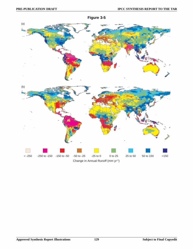
129
PRE-PUBLICATION DRAFT IPCC SYNTHESIS REPORT TO THE TAR
Approved Synthesis Report Illustrations Subject to Final Copyedit
< -250
(a)
(b)
-250 to -150 -150 to -50 -50 to -25 -25 to 0 0 to 25 25 to 50 50 to 150 >150
Change in Annual Runoff (mm yr-1)
Figure 3-5

130
PRE-PUBLICATION DRAFT IPCC SYNTHESIS REPORT TO THE TAR
Approved Synthesis Report Illustrations Subject to Final Copyedit
"��������������� ����������� � ������������������ ������������� �
�� ���/�� �;�������� �(.:.�
�
��
���
���
���
���
�������� �������
$����������������
������� �������
<��!���� !� � .�-�. ������!� &.�-�.� ��!�
Figure 3-6

131
PRE-PUBLICATION DRAFT IPCC SYNTHESIS REPORT TO THE TAR
Approved Synthesis Report Illustrations Subject to Final Copyedit
(�64 57":5;" 2�+
(�64 57":5;" 2�+
6�!!���.�1� �)��
$����)��1� �)��
$����������)���1� �)��
6�!!��) ���������.��1� �)��
$����������)���1� �)��
$#�)�����)���1� �)��
� � � ������������ ���
�� ���������������� ��� �
� � � ������������ ���
&�)
& )
&�)
�� ��������� ������������� ��� �
�� ���������������� ������������ ��� �
<��-��#!��.�� ��
'�1��.�� ��
<��-��#!��.�� ��
'�1��.�� ��
(�64 57":5;" 2�+
$����)��1� �)��
$����������)���1� �)��
$������.�1� �)��
$������������.�1� �)��
� � � ������������ ���
<��-��#!��.�� ��
'�1��.�� ��
Figure 4-1

132
PRE-PUBLICATION DRAFT IPCC SYNTHESIS REPORT TO THE TAR
Approved Synthesis Report Illustrations Subject to Final Copyedit
!���� ���������������� �
'� ���� ������ ��
������������
���������
�� ����������
!���� ���������������� �
����������������� ��
� ��������������� � ���
Figure 4-2

133
PRE-PUBLICATION DRAFT IPCC SYNTHESIS REPORT TO THE TAR
Approved Synthesis Report Illustrations Subject to Final Copyedit
Figure 4-3

134
PRE-PUBLICATION DRAFT IPCC SYNTHESIS REPORT TO THE TAR
Approved Synthesis Report Illustrations Subject to Final Copyedit
���� .�����!� �����-��� ������������� �&�0;999A�,�
$�=�������;2;!�����.�� .� ���!�)���������� +����������?���� �(����#.!�������! ��� ����������� �&�0;9A�+����������?���� �(2���#.!�������! ��� ��������� �&�0;9A�
5��������� �#��������!��������(�����!����������� �&��0;9A�
9���� �!������!�������������� �#����) ����&�0;9A���� �.�-�.������!�������������� �#����) ����&�0;9A�,��
+� �!��������)� �� ���(�������)���������� ������������ �&�0;9A�,��
"������ ������������
�������������
����������������
5�.�� ��* ���������. ��!����)��)�(����������� �&�0;9A�6��������. ��!���������� �&�0;9A�,�0;99A�4�� %�����. ���� ���� .���������� �&�0;9A�
�������������������
() ������������%����&#!�����)��.����!�������� �&�0;999A�,�,�() ���������%&!#��.%����)��.����!��������� �&�0;999A�,�,�9��� !��#��#������������ �&�0;999A�,�
�� ���� ������������������������� ��������
������������ ������������
��� ���� ����� ��� ��� ���
B�� �
� ������>�&�� ��������� �)
(������!!���!��� /.����0..���� �
(���!� ��.�* ����A0..����=..���� �
+����� �#���!� ��.�* ����A���������� ���
�� &.�-�.���!���#������)��� .�=� �!���A���� ��������������
�� &.�-�.���!���#�����������.����A���� ����������
+�� % ����%� �! �,�����%� �!
�+(������ ����/������ ��� �/����������������������� ������������ ����������� �� ������
$����������� ������ ������������� ����C���� ���
(������!!���!
Figure 5-1
Figure 5-2

135
PRE-PUBLICATION DRAFT IPCC SYNTHESIS REPORT TO THE TAR
Approved Synthesis Report Illustrations Subject to Final Copyedit
�
�
�
�
�
�+(����������&������ �0)
���� ���� ���� ����
��
��
���� ���� ���� ����
�+(������ �����&���)
���
���
���
���
���
���
���
���� ���� ���� ����
����� ��� �������&7�)
�
�
�
�
(��!� ���(������!!���!� ��%� �������.�-�. "��!!���!�� �)����!� ��.�*��(����������� ����� ���������
�
�+(��������� "������ ����+(������ ����� ����� ��� �� ������
������������� ���D�������������� ������� ���D�������� ����������+(
�� �
�� ���������
����
�����������4��������
�������
" � � � � � � � � � � + (
����������*������ �������7��%�� !��.�!!��) ����%� �
8 !����������%� �!
�.�1�����������%� �!
7��%�!.�1�������) ������%� �!
#��������
�������������� ��������������� �������
Figure 5-3
Figure 5-4

136
PRE-PUBLICATION DRAFT IPCC SYNTHESIS REPORT TO THE TAR
Approved Synthesis Report Illustrations Subject to Final Copyedit
��� ��
���
��������� �������������� �������� ��������������
&��
&��
&�
&�
&�
&�
�
�
�
���� ���� ���� ���� ����
6<D939��4;7$7"(�4"+:98894
2%����
����
������ �0
���
�
�,���
�,���
�,���
�,���
���� ���� ���� ���� ����
+���� ����
������������?��
$����� �0
?����������
�� �� �������?��
����� ���� �������#������+(����������� �������������� ���
<����������088.�?6�6������ �����E
F���
F<<<A�<�1���<#��) !��< ���%
+���� ����
�+(����������&������) �#��&��������)
�������� ��!
8�������-��������
D � �
����
����
����
����
����
����
�
����
����
���� ����
����
����
������������
Figure 5-5
Figure 5-6

137
PRE-PUBLICATION DRAFT IPCC SYNTHESIS REPORT TO THE TAR
Approved Synthesis Report Illustrations Subject to Final Copyedit
��� ������ ����
��
��
��
��
��
%�������� ���������� ���������������������� ����������������� ���
� ������� ������� ������������������� ����� �088.�(0..
����������� ���D������������&�����)
��� ������ ����
����������
����������� ���D������������&�����)
��
��
@����� ���������� ���� ���������� �������������� �������&G)
%�������� ���������� ��������������������� ����������������� ���
� ������� ������� ������������������� ����� �088.�(0..
"����� ���������� ��������������
@����� ���������� ���� ���������� ������������� �������&G)
&�)
& )
! � � � + % � � " @ @ B � " � ! � � 4 � # � @ � 4 � @ �
! � � � + % � � " @ @ B � " � ! � � 4 � # � @ � 4 � @ �
Figure 5-7

138
PRE-PUBLICATION DRAFT IPCC SYNTHESIS REPORT TO THE TAR
Approved Synthesis Report Illustrations Subject to Final Copyedit
���� ���� �����
�
�
��
��
��
����������������
��
��
��
�
�
�&�)��+(����������&����)
���� ���� �����
�
�
����������������
�
�
�
&�)���� ������������ ��� �������&7�)
���� ���� �������
����������������
���
�& )��+(������ �����&���)
���
���
���
���
���
�,���
�,���"(
"0<
<0
"("0<
<0
"(
"0<
<0
�
�
0:"�����
'%��� ������
0:"����0:"����
0:"����0:"����
�%������� ���
��� ������
��������/������ �����/��������� ��� ���������� ��������������� ������ ���D�������������� ��+(������ �����
Figure 6-1

139
PRE-PUBLICATION DRAFT IPCC SYNTHESIS REPORT TO THE TAR
Approved Synthesis Report Illustrations Subject to Final Copyedit
�
�
�
�
�
��
���������+(���� ���D�����������&���)
����� ��� ������� �����������088.�&7�)
�� ������������ ��������� ��������������������� �������������� ������� �����
��� ���D�������� ��������� ������������
,2. 22. 92. 12. :2. 82. 0/...�
�
�
�
�
����� ��� �����
����� �(0..
����� ��� ���������C���� ���
Figure 6-2
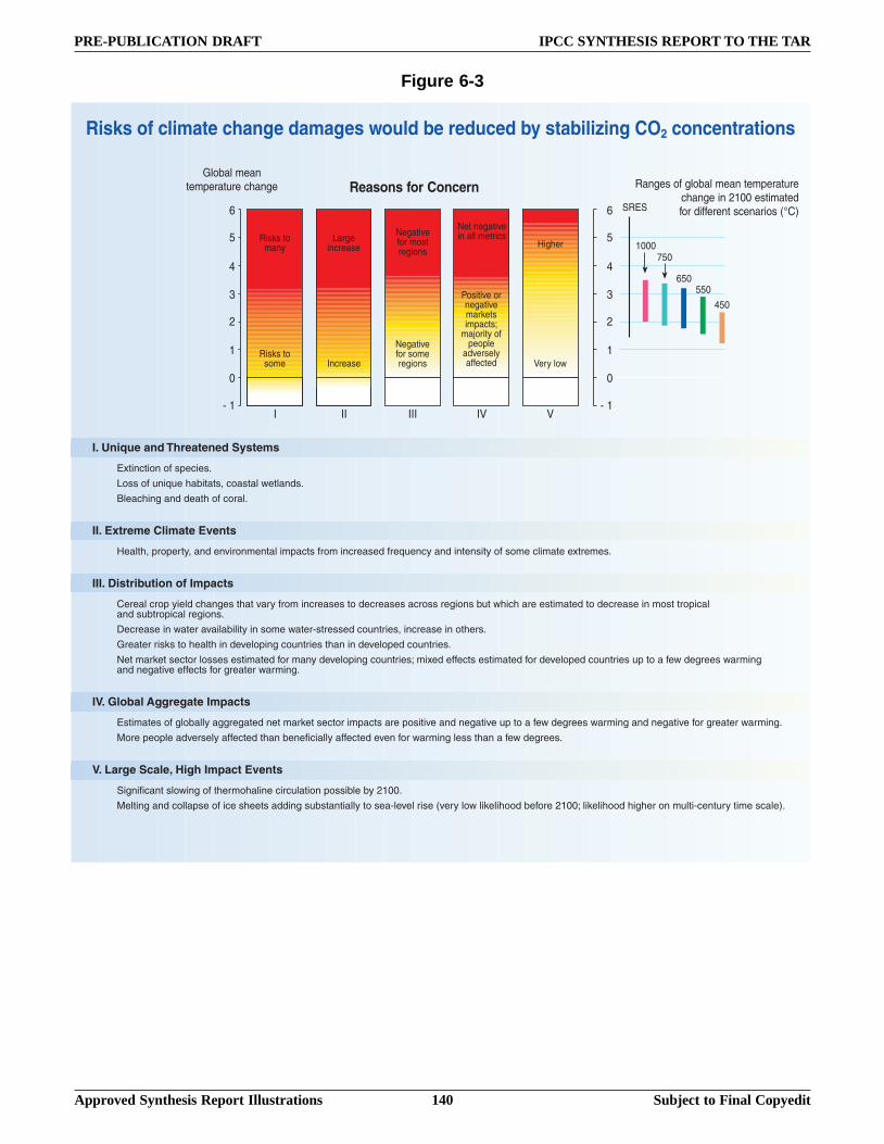
140
PRE-PUBLICATION DRAFT IPCC SYNTHESIS REPORT TO THE TAR
Approved Synthesis Report Illustrations Subject to Final Copyedit
���
������
���
�:"�
����
�6�?�C������� ��������������
"=������������!�����!
6�!!����#��C#��) ��� �!,��� !� .�1��. ��!
3.� �)���� ����� �)������� .
��6��*� �����������������
2� .�),��������%,� �����-�������� .���� ��!����������� !������C#���%� ��������!��%����!�����.�� ����=�����!
���6�#��� � ���������������
(��� .������%��.���) ���!��) ��- �%����������� !�!��������� !�!� ���!!�������!��#��1)��)� ����!��� ������������ !�������!�������� . ���!#������� .�������!
4���� !�����1 ���� - �. ��.��%����!����1 ���&!���!!�����#�����!,������ !�������)��!
;�� ������!/!����)� .�)������-�.��������#�����!��) �������-�.�������#�����!
'���� �/���!������.�!!�!��!��� ��������� �%���-�.��������#�����!B���=���������!��!��� ����������-�.�������#�����!�#����� ���1�������!�1 ����� ������ ��-��������!�������� ����1 �����
�46���� ���"�� �������������
"!��� ��!�����.�� ..%� ����� ��������� �/���!��������� ��!� �����!���-�� ������ ��-��#����� ���1�������!�1 ������ ������ ��-��������� ����1 �����
$��������.�� �-��!�.%� ���������) ���������� ..%� ���������-�������1 ������.�!!��) �� ���1�������!
46�@� ��������/�!���������������
�������� ���!.�1��������)����) .��������#. �������!!��.���%�����
$�.����� �����.. �!���������!)���!� ������!#�!� ��� ..%����!� &.�-�.���!��-��%�.�1�.�/�.�)���������������B�.�/�.�)����)��)�������#.��&����#�%������!� .�
%����������������������������������� �� ������� ����� ���D����+(������ �����
%�������� ����� ;.�� .��� �
������ �#����) ��� : ���!�����.�� .��� �������� �#���) �������������!��� �����������������!��� ���!�G(
:�!/!���� �%
6 �������� !�
'�� ��-�������!�������!
'������ ��-���� ..�������!
2��)��
:�!/!���!��� 9���� !�
'�� ��-�����!���������!
<�!���-������� ��-�� �/��!��� ��!B� @����%�������.�
�-��!�.% ������� 7��%�.�1
9 99 999 97 7
�
�
�
�
�
�
�
&��
�
�
�
�
�
�
�
&��
Figure 6-3

141
PRE-PUBLICATION DRAFT IPCC SYNTHESIS REPORT TO THE TAR
Approved Synthesis Report Illustrations Subject to Final Copyedit
$� ������������5��# .�#!�������-�������� ..%�!�#�����)��.����!� ����� �����!
����������������>�5���� �)����%��� ��������� �/��!,����#���������� �/���� �.#��!,� ������� !������ ��� .� ������)��.��%��� �!���!
����������������������>�5���� �)����% ������������) ���!������) -��#�,�.���!�%.�!,!��� .�!��#��#��,� �����!���#����!
��������������������>�5���� �)����%���.������������)��.��%��) ��) ! .�� �%�����������!�� ���
����������������+)������� .�#�������#��,�� %�!)�����-�������
���������
"��������������
$�����������������
������������������������������
65(H��8�(�$<"+9+9�'
+:54"�35::9":�
�'4"89'"4<:�<":+I�:9;2+�
9'54"E�5+"9'8�:$5+9�'
��(956�'�:$�
9'49794�56�2539+�
5++9+�4"�
756�"�
7"�+"4�9'+":"�+�
69$9+"4�5759653969+I5'4�H'�06"4;"
53��+�'"0+"(2'�6�;9"�
:"�"5:(2,�4"7"6�<$"'+4"$�'�+:5+9�'��8'"0�+"(2'�6�;9"�
'"+0�:H�(:"5+9�'
(�$$�'9+I�9'7�67"$"'+9'�<�69(I$5H9';
56+":'5+97"�698"�+I6"�
"4�(5+9�'
<�69(I�9'9+95+97"�
9'�+9+�+9�'56�:"8�:$
��3�94I�:"8�:$
$9(:�&(:"49+
:�:56�"6"(+:989(5+9�'
(��<":5+97"�5;:""$"'+�
'"0�$"5��:"�+5J"�,�9'("'+97"�
$�6+9&�5'43965+":56�<:�D"(+�
"J5$<6"���8�35::9":� �H"$�@���+��"���+-��+�+4�%�+$��<"%%��%�
Figure 7-1

142
PRE-PUBLICATION DRAFT IPCC SYNTHESIS REPORT TO THE TAR
Approved Synthesis Report Illustrations Subject to Final Copyedit
��
��
��
��
��
�
� �;�����������#�������������� ������������"�*�������� ������������ �(.0.�� ������ ���������
��
��
��
��
��
��
��
���
���
���
���
���
���
���
���
���
���
���
���
���
���
���
���
���
���
���
���
���
���
���
���
�� �����������#��������������� �(.0.
�����/�"��� ����/���-���I�����
?����������� +��#����� �������� ���
F���
%������������������ ��������� ���
5�!�������������� ���� .��� ������� �������!!���!����)�!A�� �)���������#!��� /��)�����!����������#�����
8#..�5���=�3��� ��������� ��������!!���!���)�!����������
+)���)�����#����!����� �)�� ������!�����)��)��)�!�,��� �,� ��.�1�!�����@������!�������)��!���������.!
D � �
5#!�� .� '�1
K� . ��
�"(4���#�����!���"#����
( � �
��������� ��!
���
���
���
���
���
�
���
������
��
���
��
���
��
���
���
���
���
��
����
���
������
��
���
��
088.�?������� � ��� ����
�����/�"��� ����/���-���I�����
?����������� +��#����� �������� ���
F���
���
����
���
����
&�)��#��������
& )�$� ���������
Figure 7-2

2
18
16
14
12
10
8
6
4
What will it cost to stabilize CO2 concentrations?
0
Gt C
1600
1400
1000
800
600
400
200
0
1200
714
1043
1239
1348
Trillions (1012) of 1990 U.S. dollars
1800
Cumulative carbon emissionsbetween 1990 and 2100
Models : FUNDSWRE
MERGE MiniCAMSWRE
SWRE
450 ppmv 550 ppmv 650 ppmv 750 ppmv
Scenarios :
Figure 7-3: The mitigation costs (1990 US$, present value discounted at 5% per year for the period 1990 to 2100) of stabilizing CO2 concentrations at 450 to 750 ppmv are calculated using three global models, based on different model-dependent baselines. Avoided impacts of climate change are not included. In each instance, costs were calculated based on two emission pathways for achieving the prescribed target: S (referred as WGI emissions pathways in WGIII TAR) and WRE as described in response to Question 6. The bars show cumulative carbon emissions between the years 1990 and 2100. Cumulative future emissions until carbon budget ceiling is reached are reported above the bars in Gt C.
CORRECTIONAn error occurred in all language versions of the TAR Synthesis Reportin the vertical scale of Figure 7-3. The correct figure is shown below:

143
PRE-PUBLICATION DRAFT IPCC SYNTHESIS REPORT TO THE TAR
Approved Synthesis Report Illustrations Subject to Final Copyedit
�
��
��
��
��
��
�
�
�
'���������������������� ���D���+(������ �����A
�
����
����
����
����
���
���
���
���
�
����
���
����
��������
� �������&0.0()����088.�?6�6������ �
����
(#�#. ��-��� ��������!!���!���1��������� �������
$������> �?-#�0:"
$�%�� $���"$�0:"
�0:"
,2.����� 22.����� 92.����� 12.�����
���� ����>
,2. 22. 92. 12.
���������+(���� ���D�����������&���)
�� ������� �������� ����������� ������
�
��
��
��
��
��
��
��
��
�� ���� ���>
5�3
5�+
5�89
5�
3�
3�
��� ������ �����#�� ���������������� �(.2.
Figure 7-3
Figure 7-4

144
PRE-PUBLICATION DRAFT IPCC SYNTHESIS REPORT TO THE TAR
Approved Synthesis Report Illustrations Subject to Final Copyedit
�
�����
�����
�����
�����
�����
�����
�����
���
����
+�����
����
!���� �����������������������0:9.�088:
<0"0�
<(
"0<
"(
"0��
'%�=2.
'%�,2.
'%�22.
'%�92.
'%�12.
'%�0...
%��� ������� ���� ��� �������� �%������� ��� ��� ���D��������� ���
��.
(� .
; !
�� ���������������� ��� ������� ���� ��������� ����������� ������������������ ����������/��������������������� ������������ ����� �������%������� �������"%���� ���D��������� ������������������ �(0..
(��-������ .���!��-�!
(��-������ .���!�#���!�#������!��� ��
�����-������ .���!��-�!� �����!�#���!
Figure 7-5

145
PRE-PUBLICATION DRAFT IPCC SYNTHESIS REPORT TO THE TAR
Approved Synthesis Report Illustrations Subject to Final Copyedit
#��� ��������� �� ��� �
�����������
@������� ������������������������� ���� �������������
"� C������
<������ ����
'���
�� ������ ���D�����������
Figure 8-1

146
PRE-PUBLICATION DRAFT IPCC SYNTHESIS REPORT TO THE TAR
Approved Synthesis Report Illustrations Subject to Final Copyedit
��������������������
�������������������
?������� ���� ��� �
@������ ������
<������ ��������
�����������
'������������.�* ����
2%���.����� ��(����) ���!
� .���* ���� ������!���
8����.��%.�!!
"=���
!���� ����
6�!!� ����� ����� �������) ��� �!
6�!!��������!����������-��!��%
Figure 8-2
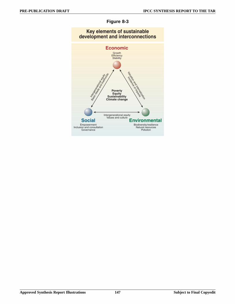
147
PRE-PUBLICATION DRAFT IPCC SYNTHESIS REPORT TO THE TAR
Approved Synthesis Report Illustrations Subject to Final Copyedit
�������
��� ������������"���1������
9��.#!���� ������!#.� ����;�-��� ���
3����-��!��%L��!�.�����' �#� .���!�#���!
<�..#����
;��1�)"��������%�� ��.��%
���� ���C����
������� �����������������
9��������� ���� .��C#��%7 .#�!� ����#.�#��
9��������� ���� .��C#��%
3 !�������!� ���.�-�.�)���!
7 .# ����� ��������� .�* ����
9��������������� ��!
J��������������������� ������������������� ��������
Figure 8-3
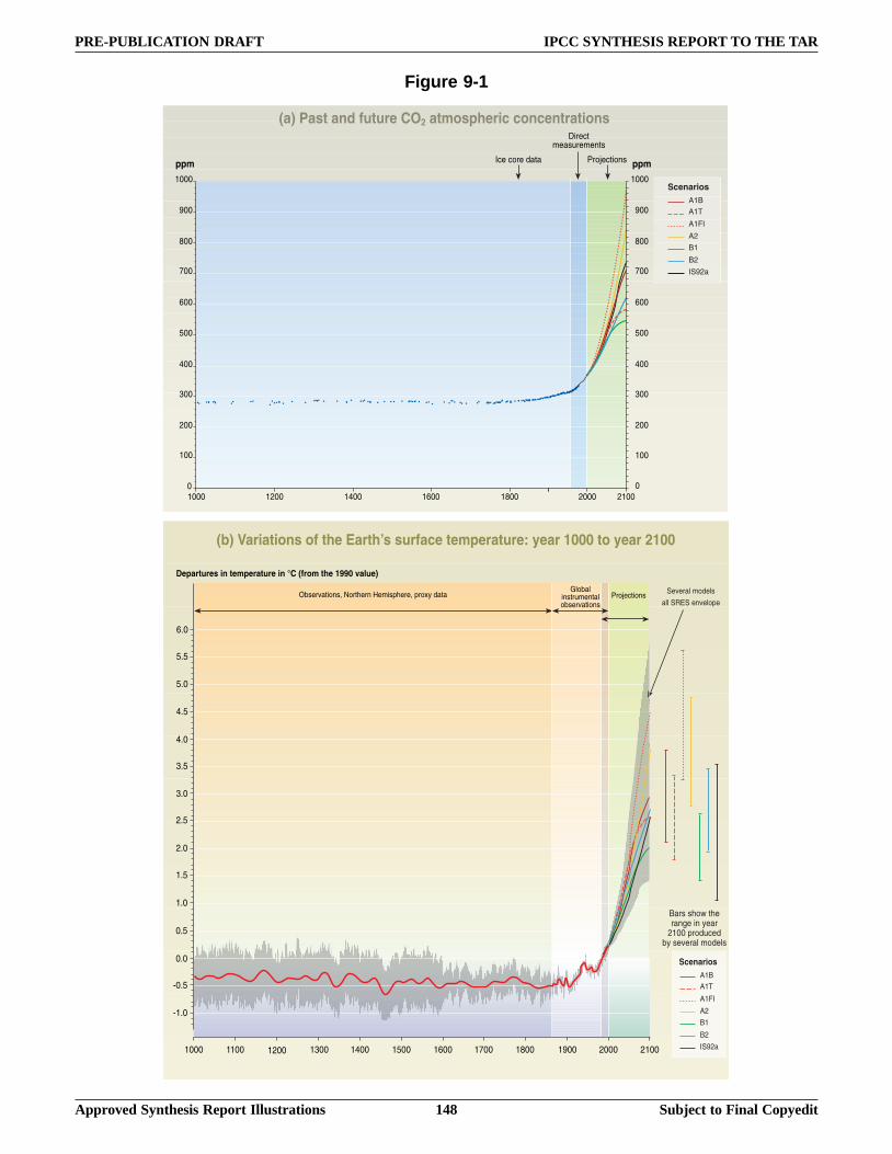
148
PRE-PUBLICATION DRAFT IPCC SYNTHESIS REPORT TO THE TAR
Approved Synthesis Report Illustrations Subject to Final Copyedit
&�)������������� ���+(�������� �������� �����
���
���
���
���
���
���
���
���
����
���� ���� ���� ���� ���� ����
5�35�+
5�89
5�3�
3�
9���
���� ���
����
���
���
���
���
���
���
���
���
����
���
�
��� ���
�
9��������� �
4������� !#������!
<��@������! ���
5�35�+
5�89
5�3�
3�
9���
���� ���
3 �!�!)�1��)�� �������%� ����������#���
�%�!�-�� .�����.!
��-�� .�����.!
..��:"����-�.���
���� ���� ���� ���� ���� ����
&��
��
& )�4� ��������������� �5���� ���������� ��� �>���� �0...������� �(0..
#��� �� ���������� ��� ����7��&� ������088.������)
���� ���� ���� ���� ���� ����
&��
��!��- ����!,�'���)����2���!�)���,����=%�� � ;.�� .
��!��#���� .��!��- ����!
<��@������!
��
��
��
��
��
��
��
��
��
��
��
��
Figure 9-1


