Click Here Full Article Spatial and temporal variability ... · Spatial and temporal variability of...
13
Spatial and temporal variability of droughts in Portugal Joa ˜o Filipe Santos, 1 Inmaculada Pulido-Calvo, 2 and Maria Manuela Portela 3 Received 2 April 2009; revised 4 June 2009; accepted 11 September 2009; published 4 March 2010. [1] An analysis of droughts in mainland Portugal based on monthly precipitation data, from September 1910 to October 2004, in 144 rain gages distributed uniformly over the country is presented. The drought events were characterized by means of the Standardized Precipitation Index (SPI) applied to different time scales (1, 6, and 12 consecutive months and 6 months from April to September and 12 months from October to September). To assess spatial and temporal patterns of droughts, a principal component analysis (PCA) and K-means clustering (KMC) were applied to the SPI series. In this way, three different and spatially well-defined regions with different temporal evolution of droughts were identified (north, central, and south regions of Portugal). A spectral analysis of the SPI patterns obtained with principal component analysis and clusters analysis, using the fast Fourier transform algorithm (FFT), showed that there is a manifest 3.6-year cycle in the SPI pattern in the south of Portugal and evident 2.4-year and 13.4-year cycles in the north of Portugal. The observation of the drought periods supports the occurrence of more frequent cycles of dry events in the south (droughts from moderate to extreme approximately every 3.6 years) than in the north (droughts from severe to extreme approximately every 13.4 years). These results suggest a much stronger immediate influence of the NAO in the south than in the north of Portugal, although these relations remain a challenging task. Citation: Santos, J. F., I. Pulido-Calvo, and M. M. Portela (2010), Spatial and temporal variability of droughts in Portugal, Water Resour. Res., 46, W03503, doi:10.1029/2009WR008071. 1. Introduction [2] Droughts are still among the least understood extreme weather events affecting large worldwide areas and having serious impacts on society, environment, and economy. Droughts are complex natural hazards that distress significant areas of the world every year, though with different severi- ties. In Europe the drought of 2003 affected 19 countries with a total estimated cost that exceeded 11.6 billion Euros (http://www.euraqua.org). The costs estimated for Portugal during the 2005 drought were 285 million Euros, with half of this amount related to losses from the hydroelectric power production sector; many other sectors such as agri- culture, forestry, and water supply also suffered severe losses. According to the Portuguese Water Institute, in 2005, 80% of the country experienced the worst drought in 60 years (http://www.eumetsat.int/Home/Main/Media/ News/005280?l=en). In the southern part, which is also the driest part, agriculture represents the main activity sector, so high correlation must be expected between drought occurrence and agricultural outputs. [3] Shortage of water poses a great threat to nature, quality of life, and economy. Increasing water demands lead to confiicts among competing water users that are most pronounced during drought periods [Hisdal and Tallaksen, 2003]. The study of the climate variability may contribute to a more correct management of such extreme climatic occurrences. Recently, there has been debate on the appar- ent increase, regarding the event frequency and the affected area, of droughts and on the possible physical causes of such circumstance. In the Mediterranean basin, if precipi- tation decrease pointed out by the climate change models [Bates et al., 2008] is confirmed, the consequences would be severe in terms of the progressive scarcity of surface water due to the high demand for agricultural, industrial, and tourist activities and of the intensification of erosion and desertification processes [Lo ´pez-Bermu ´dez and Sa ´nchez, 1997; New et al., 2002; Vicente-Serrano et al., 2004]. [4] To assess the drought occurrence in mainland Portugal and to understand the historical and recent climatic vari- ability, it is worthwhile to study the long-term time series of precipitation regarding their nonhomogeneous climatic and hydrological conditions. For very restricted areas, some authors have analyzed the drought phenomenon by com- paring results from well-known scientific indices, such as the Standardized Precipitation Index (SPI) and the Palmer Drought Severity Index (PDSI) [Paulo and Pereira, 2006; Domingos, 2006], by studying the intensity and frequency of drought events [Pires, 2003], and by predicting drought categories [Moreira et al., 2006, Paulo and Pereira, 2007, 2008]. 1 Departamento Engenharia, ESTIG, Instituto Polite ´cnico de Beja, Beja, Portugal. 2 Departamento Ciencias Agroforestales, EPS, Campus Universitario de La Ra ´bida, Universidad de Huelva, Palos de la Frontera, Spain. 3 Departamento Engenharia Civil, SHRH, Instituto Superior Te ´cnico, Lisbon, Portugal. Copyright 2010 by the American Geophysical Union. 0043-1397/10/2009WR008071$09.00 W03503 WATER RESOURCES RESEARCH, VOL. 46, W03503, doi:10.1029/2009WR008071, 2010 Click Here for Full Article 1 of 13
-
Upload
nguyenliem -
Category
Documents
-
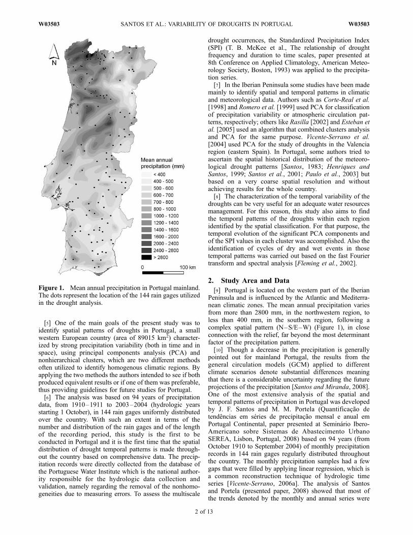
view
223 -
download
0
Transcript of Click Here Full Article Spatial and temporal variability ... · Spatial and temporal variability of...
Spatial and temporal variability of droughts in Portugal
Joao Filipe Santos,1 Inmaculada Pulido-Calvo,2 and Maria Manuela Portela3
Received 2 April 2009; revised 4 June 2009; accepted 11 September 2009; published 4 March 2010.
[1] An analysis of droughts in mainland Portugal based on monthly precipitation data,from September 1910 to October 2004, in 144 rain gages distributed uniformly overthe country is presented. The drought events were characterized by means of theStandardized Precipitation Index (SPI) applied to different time scales (1, 6, and12 consecutive months and 6 months from April to September and 12 months fromOctober to September). To assess spatial and temporal patterns of droughts, a principalcomponent analysis (PCA) and K-means clustering (KMC) were applied to the SPI series.In this way, three different and spatially well-defined regions with different temporalevolution of droughts were identified (north, central, and south regions of Portugal). Aspectral analysis of the SPI patterns obtained with principal component analysis andclusters analysis, using the fast Fourier transform algorithm (FFT), showed that there is amanifest 3.6-year cycle in the SPI pattern in the south of Portugal and evident 2.4-yearand 13.4-year cycles in the north of Portugal. The observation of the drought periodssupports the occurrence of more frequent cycles of dry events in the south (droughts frommoderate to extreme approximately every 3.6 years) than in the north (droughts fromsevere to extreme approximately every 13.4 years). These results suggest a much strongerimmediate influence of the NAO in the south than in the north of Portugal, although theserelations remain a challenging task.
Citation: Santos, J. F., I. Pulido-Calvo, and M. M. Portela (2010), Spatial and temporal variability of droughts in Portugal, Water
Resour. Res., 46, W03503, doi:10.1029/2009WR008071.
1. Introduction
[2] Droughts are still among the least understood extremeweather events affecting large worldwide areas and havingserious impacts on society, environment, and economy.Droughts are complex natural hazards that distress significantareas of the world every year, though with different severi-ties. In Europe the drought of 2003 affected 19 countrieswith a total estimated cost that exceeded 11.6 billion Euros(http://www.euraqua.org). The costs estimated for Portugalduring the 2005 drought were 285 million Euros, with halfof this amount related to losses from the hydroelectricpower production sector; many other sectors such as agri-culture, forestry, and water supply also suffered severelosses. According to the Portuguese Water Institute, in2005, 80% of the country experienced the worst droughtin 60 years (http://www.eumetsat.int/Home/Main/Media/News/005280?l=en). In the southern part, which is alsothe driest part, agriculture represents the main activitysector, so high correlation must be expected betweendrought occurrence and agricultural outputs.
[3] Shortage of water poses a great threat to nature,quality of life, and economy. Increasing water demandslead to confiicts among competing water users that are mostpronounced during drought periods [Hisdal and Tallaksen,2003]. The study of the climate variability may contribute toa more correct management of such extreme climaticoccurrences. Recently, there has been debate on the appar-ent increase, regarding the event frequency and the affectedarea, of droughts and on the possible physical causes ofsuch circumstance. In the Mediterranean basin, if precipi-tation decrease pointed out by the climate change models[Bates et al., 2008] is confirmed, the consequences wouldbe severe in terms of the progressive scarcity of surfacewater due to the high demand for agricultural, industrial,and tourist activities and of the intensification of erosion anddesertification processes [Lopez-Bermudez and Sanchez,1997; New et al., 2002; Vicente-Serrano et al., 2004].[4] To assess the drought occurrence in mainland Portugal
and to understand the historical and recent climatic vari-ability, it is worthwhile to study the long-term time series ofprecipitation regarding their nonhomogeneous climatic andhydrological conditions. For very restricted areas, someauthors have analyzed the drought phenomenon by com-paring results from well-known scientific indices, such asthe Standardized Precipitation Index (SPI) and the PalmerDrought Severity Index (PDSI) [Paulo and Pereira, 2006;Domingos, 2006], by studying the intensity and frequencyof drought events [Pires, 2003], and by predicting droughtcategories [Moreira et al., 2006, Paulo and Pereira, 2007,2008].
1Departamento Engenharia, ESTIG, Instituto Politecnico de Beja, Beja,Portugal.
2Departamento Ciencias Agroforestales, EPS, Campus Universitario deLa Rabida, Universidad de Huelva, Palos de la Frontera, Spain.
3Departamento Engenharia Civil, SHRH, Instituto Superior Tecnico,Lisbon, Portugal.
Copyright 2010 by the American Geophysical Union.0043-1397/10/2009WR008071$09.00
W03503
WATER RESOURCES RESEARCH, VOL. 46, W03503, doi:10.1029/2009WR008071, 2010ClickHere
for
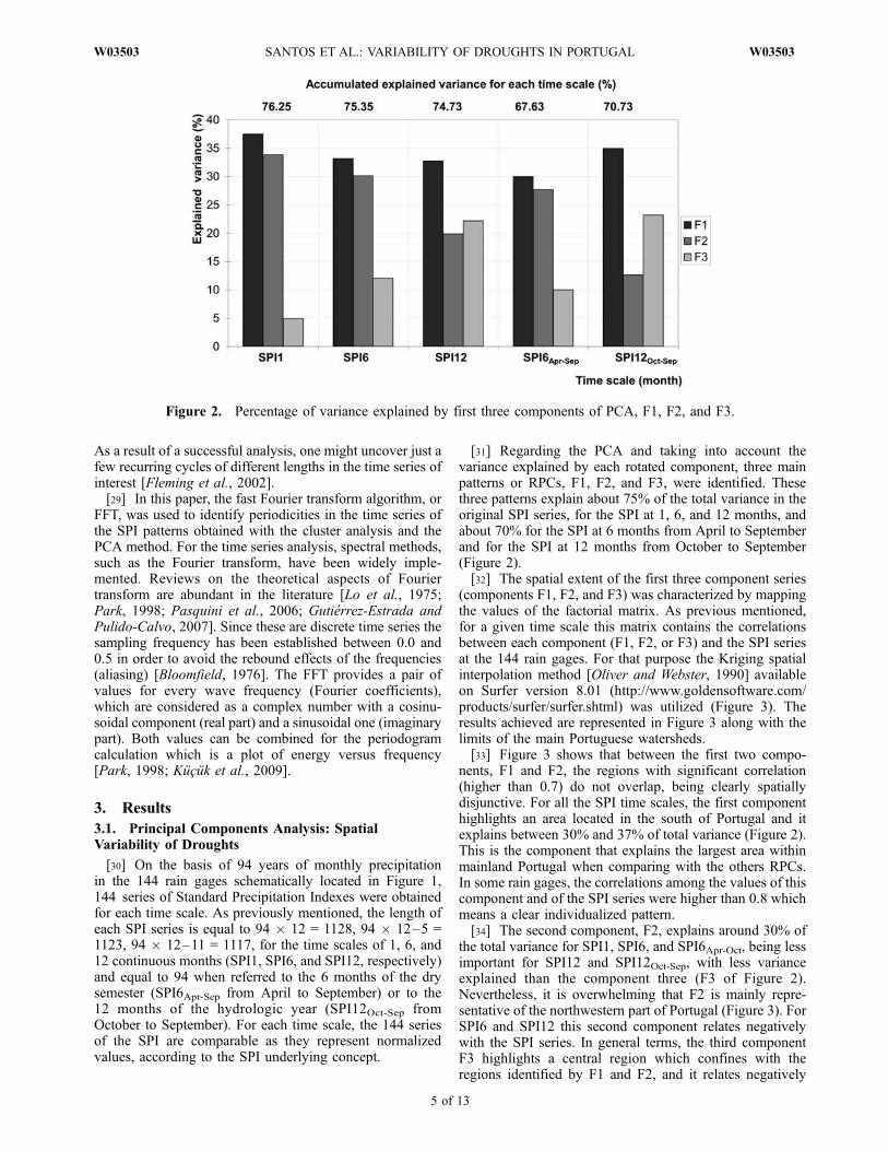
FullArticle
1 of 13
[5] One of the main goals of the present study was toidentify spatial patterns of droughts in Portugal, a smallwestern European country (area of 89015 km2) character-ized by strong precipitation variability (both in time and inspace), using principal components analysis (PCA) andnonhierarchical clusters, which are two different methodsoften utilized to identify homogenous climatic regions. Byapplying the two methods the authors intended to see if bothproduced equivalent results or if one of them was preferable,thus providing guidelines for future studies for Portugal.[6] The analysis was based on 94 years of precipitation
data, from 1910–1911 to 2003–2004 (hydrologic yearsstarting 1 October), in 144 rain gages uniformly distributedover the country. With such an extent in terms of thenumber and distribution of the rain gages and of the lengthof the recording period, this study is the first to beconducted in Portugal and it is the first time that the spatialdistribution of drought temporal patterns is made through-out the country based on comprehensive data. The precip-itation records were directly collected from the database ofthe Portuguese Water Institute which is the national author-ity responsible for the hydrologic data collection andvalidation, namely regarding the removal of the nonhomo-geneities due to measuring errors. To assess the multiscale
drought occurrences, the Standardized Precipitation Index(SPI) (T. B. McKee et al., The relationship of droughtfrequency and duration to time scales, paper presented at8th Conference on Applied Climatology, American Meteo-rology Society, Boston, 1993) was applied to the precipita-tion series.[7] In the Iberian Peninsula some studies have been made
mainly to identify spatial and temporal patterns in climaticand meteorological data. Authors such as Corte-Real et al.[1998] and Romero et al. [1999] used PCA for classificationof precipitation variability or atmospheric circulation pat-terns, respectively; others like Rasilla [2002] and Esteban etal. [2005] used an algorithm that combined clusters analysisand PCA for the same purpose. Vicente-Serrano et al.[2004] used PCA for the study of droughts in the Valenciaregion (eastern Spain). In Portugal, some authors tried toascertain the spatial historical distribution of the meteoro-logical drought patterns [Santos, 1983; Henriques andSantos, 1999; Santos et al., 2001; Paulo et al., 2003] butbased on a very coarse spatial resolution and withoutachieving results for the whole country.[8] The characterization of the temporal variability of the
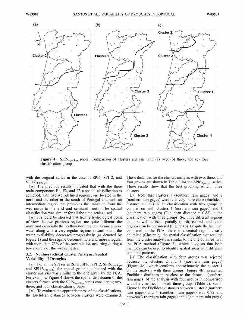
droughts can be very useful for an adequate water resourcesmanagement. For this reason, this study also aims to findthe temporal patterns of the droughts within each regionidentified by the spatial classification. For that purpose, thetemporal evolution of the significant PCA components andof the SPI values in each cluster was accomplished. Also theidentification of cycles of dry and wet events in thosetemporal patterns was carried out based on the fast Fouriertransform and spectral analysis [Fleming et al., 2002].
2. Study Area and Data
[9] Portugal is located on the western part of the IberianPeninsula and is influenced by the Atlantic and Mediterra-nean climatic zones. The mean annual precipitation variesfrom more than 2800 mm, in the northwestern region, toless than 400 mm, in the southern region, following acomplex spatial pattern (N–S/E–W) (Figure 1), in closeconnection with the relief, far beyond the most determinantfactor of the precipitation pattern.[10] Though a decrease in the precipitation is generally
pointed out for mainland Portugal, the results from thegeneral circulation models (GCM) applied to differentclimate scenarios denote substantial differences meaningthat there is a considerable uncertainty regarding the futureprojections of the precipitation [Santos and Miranda, 2008].One of the most extensive analysis of the spatial andtemporal patterns of precipitation in Portugal was developedby J. F. Santos and M. M. Portela (Quantificacao detendencias em series de precipitacao mensal e anual emPortugal Continental, paper presented at Seminario Ibero-Americano sobre Sistemas de Abastecimento UrbanoSEREA, Lisbon, Portugal, 2008) based on 94 years (fromOctober 1910 to September 2004) of monthly precipitationrecords in 144 rain gages regularly distributed throughoutthe country. The monthly precipitation samples had a fewgaps that were filled by applying linear regression, which isa common reconstruction technique of hydrologic timeseries [Vicente-Serrano, 2006a]. The analysis of Santosand Portela (presented paper, 2008) showed that most ofthe trends denoted by the monthly and annual series were
Figure 1. Mean annual precipitation in Portugal mainland.The dots represent the location of the 144 rain gages utilizedin the drought analysis.
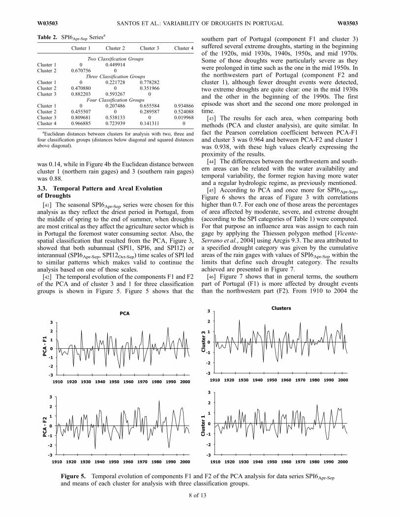
2 of 13
W03503 SANTOS ET AL.: VARIABILITY OF DROUGHTS IN PORTUGAL W03503
statistically meaningless, explained by the natural temporalvariability of the precipitation. A pronounced and general-ized decrease in the precipitation was only detected inMarch. However, the high spatial heterogeneity of theprecipitation makes it difficult to establish an overall pat-tern. The same precipitation data was used in this paper toanalyze droughts based on the Standardized PrecipitationIndex (SPI) [Guttman, 1999; McKee et al., presented paper,1993].
2.1. Drought Index Calculation
[11] As previous mentioned, in the present paper theStandardized Precipitation Index (SPI), originally developedby McKee et al. (presented paper, 1993) was adopted toassess the drought in mainland Portugal. The SPI, which hasbecome the most popular drought index during the last2 decades [Vicente-Serrano, 2006a], has several advantages,such as (1) great flexibility, as it can be applied at differenttime scales [Edwards and McKee, 1997]; (2) less complex-ity, comparatively to other indexes, as it requires relativelysimple and well set calculations [Guttman, 1998, 1999];(3) adaptability to hydroclimatologic variables besidesprecipitation [Seiler et al., 2002; Vicente-Serrano andLopez-Moreno, 2005; Lopez-Moreno et al., 2009]; and(4) suitability to spatial representation, allowing comparisonbetween areas within the same region, as it is a normalizedindex [Hayes et al., 1999; Lloyd-Hughes and Saunders,2002; Vicente-Serrano, 2006a, 2006b; Bordi et al., 2004;Loukas and Vasiliades, 2004].[12] The SPI calculated at 1 month is mainly a meteoro-
logical drought index [Hayes et al., 1999], at time scalesbetween 3 and 6 months it can be considered an agriculturaldrought index [Hayes et al., 1999; Yamoah et al., 2000], andat time scales between 6 and 12 months it is considered ahydrological drought index [Hayes et al., 1999; Komuscu,1999; Vicente-Serrano, 2006a], becoming useful for moni-toring the surface water resources [Vicente-Serrano andLopez-Moreno, 2005].[13] To ascertain the variability of both spatial and
temporal patterns for different types of droughts, in theanalysis carried out for mainland Portugal the SPI was usedat different time scales, namely at 1 (SPI1), 6 (SPI6), and12 (SPI12) consecutive months; at 6 months of the dry season(April to September, SPI6Apr-Sep); and at 12 months of thehydrologic year (October to September, SPI12Oct-Sep). SPI1,SPI6, and SPI12 account for the subannual variability ofdroughts and SPI6Apr-Sep and SPI12Oct-Sep account for theinterannual variability.[14] Originally, McKee et al. (presented paper, 1993)
adjusted a Gamma distribution function to the precipitation
series to compute the SPI index. Afterward, other authorstested several distributions based on different time scalesand concluded that the Pearson type III distribution ensuredthe best fit. This circumstance can be explained by thehigher flexibility of the Pearson type III distribution givenby its three parameters in comparison with the Gammadistribution with only two parameters [Guttman, 1999;Ntale and Gan, 2003; Vicente-Serrano, 2006a]. A PearsonIII distributed random variable x is written as
f xð Þ ¼ 1
a G bð Þx� ga
� �b�1e�
x�gað Þ ð1Þ
where a, b, and g are shape, scale, and origin parameters,respectively, for values of x such that x > 0. The term G(b) isthe Gamma function of b. In the applications carried outx denotes precipitation and the parameters of the Pearsontype III distribution were estimated using the L-momentsmethod. According to Sankarasubramanian and Srinivasan[1999], the L-moments method has advantages regardingthe conventional moments, especially when the size of thesample increases, and with highly biased distributions.[15] To compute the SPI series, the detailed formulation
provided by Vicente-Serrano [2005, 2006b] was followed.The drought categories adopted the SPI limits proposed byAgnew [2000], shown in Table 1.[16] The spatial and temporal characterization of the
droughts was accomplished by means of principal compo-nent analysis (PCA) and nonhierarchical cluster analysis. Toascertain the drought patterns, both procedures were appliedto the SPI series, as many other authors have done success-fully for the same purpose [Klugman, 1978; Karl andKoscielny, 1982; Stahl and Demuth, 1999; Bonaccorso etal., 2003; Vicente-Serrano et al., 2004].
2.2. Principal Components Analysis
[17] The principal component analysis (PCA) is a com-mon way of identifying patterns in climatic data andexpressing the data in such a way as to highlight theirsimilarities and differences [Smith, 2002]. Others [Lins,1985; Tipping and Bishop, 1999; Jolliffe, 2002; Singh etal., 2009; Kahya et al., 2008a, 2008b] define the PCAmethod as a technique applied to multivariate analysis fordimensionality reduction, emphasizing patterns on data andrelations between variables and between variables andobservations. The original intercorrelated variables couldbe reduced to a small number of new linearly uncorrelatedones that explain most of the total variance [Rencher, 1998;Bonaccorso et al., 2003]. Some aspects in the use of PCAcould be found, such as (1) PCAs are not affected by thelack of independency in the original variables; (2) normalityis desirable but not essential; and (3) only an excessivenumber of zeros could cause problems, which in theapplications envisaged is not a concern [Hair et al.,2005]. As stated by Kalayci and Kahya [2006], the PCAmethod does not require normalized data sets as long as thedata are not excessively skewed; since SPI is a normalizedvariable, following the calculation procedure, there were noneeds to previously transform data, nevertheless somenormality assessment has been made previously to thePCA application.
Table 1. Drought Categories According to the SPI Valuesa
Nonexceedance Probability SPI Drought Category
0.05 >1.65 extremely wet0.10 >1.28 severely wet0.20 >0.84 moderately wet0.60 >�0.84 and <0.84 normal0.20 <�0.84 moderate drought0.10 <�1.28 severe drought0.05 <�1.65 extreme drought
aValues are from Agnew [2000].
W03503 SANTOS ET AL.: VARIABILITY OF DROUGHTS IN PORTUGAL
3 of 13
W03503
[18] Considering k variables in a given time period i, Xi,1,Xi,2, . . ., Xi,k, k principle components (PCs) are produced forthe same time period, Yi,1, Yi,2, . . ., Yi,k, using linearcombinations of the first ones, according to:
Yi;1 ¼ a11Xi;1 þ a12Xi;2 þ . . .þ a1kXi;k
Yi;2 ¼ a21Xi;1 þ a22Xi;2 þ . . .þ a2kXi;k
. . .
Yi;k ¼ ak1Xi;1 þ ak2Xi;2 þ . . .þ akkXi;k
:
8>>>>>>>><>>>>>>>>:
ð2Þ
[19] In the applications developed the variables Xi,k referto SPI series, k is equal to the number of rain gages (144)and i represents the length of SPI series in each rain gage.For SPI1, SPI6, and SPI12, i varies from 1 to 94 � 12 =1128, 1 to 94 � 12–5 = 1123, and 1 to 94 � 12–11 = 1117,respectively, and both for SPI6Apr-Sep and SPI12Oct-Sep from1 to 94.[20] In the previous combinations the Y values are
orthogonal and uncorrelated variables, such that Yi,1explains most of the variance, Yi,2 explains the reminiscentamount of variance, and so on. The coefficients of the linearcombinations are called ‘‘loadings’’ and represent theweights of the original variables in the PCs.[21] PCs extraction could be based on variance/covariance
or correlation matrix of data with {a11, a12, . . ., a1k} beingthe first eigenvector and {ak1, ak2, . . ., akk} being theeigenvector of k order. Each eigenvector includes thecoefficients of the k principal component.[22] Finally, the amount of variance explained by the first
PC is called the first eigenvalue, l1, the second is l2, so thatl1 � l2 � l3 � l4 . . . lk, since each eigenvalue representsthe fraction of the total variance in the original data andexplained by each component [Bordi and Sutera, 2001] sothat this proportion can be calculated as lj/
Plj. The analysis
of the results of PCs can be focused on the eigenvalues, onthe correlations between PCs and the original variables(factor loadings), or on the observation coordinates in thePC (factor scores). In this paper, only the correlationsbetween the original data (SPI series) and the PCs wereused for classification purposes (that is, for choosing themain PCs). Those correlations are stored in the factorialmatrix.[23] To achieve more stable spatial patterns, a rotation of
the principal components with the Varimax procedure wasapplied. This procedure provides a clearer division betweencomponents, preserves their orthogonality, and producesmore physically explainable patterns [Richman, 1986;Vicente-Serrano et al., 2004]. Kahya et al. [2008a, 2008b]referred that the rotation simplifies the spatial structure byisolating regions with similar temporal variations, being theVarimax procedure the most common orthogonal method toimprove the creation of regions of maximum correlationbetween the variables and the components. The patternsdefined in this way are referred as rotated principal compo-nents (RPCs).
2.3. Nonhierarchical Cluster Analysis
[24] The Cluster analysis technique, similarly to the PCAmethod, was chosen for its ability to divide the data set into
homogeneous and distinct groups having members withsimilar characteristics [Shukla et al., 2000; Pulido-Calvoet al., 2006]. Cluster analysis is a generic term for a varietyof statistical methods that can be used to evaluate thesimilarity of individual objects in a set. A simple examplewould be gathering a set of pebbles of different size, shape,and color from a stream shore and sorting similar pebblesinto the same pile. This is an example of physical clusteranalysis. Statistical methods of cluster analysis achieve thismathematically. The objects in such statistical methods aredata rather than real objects (e.g., pebbles).[25] Using the calculated SPI data, the rain gages should
be grouped homogeneously so that similar SPI variations atdifferent time scales will be assigned to the same group,while different variations will be grouped separately. Amathematical criterion to calculate the classification and tojudge the quality of the classification must be used. Thisquestion can be addressed by the K-means clustering(KMC) method which can reassign each observation to adifferent cluster with the nearest centroid [Rhee et al.,2008]. Gong and Richman [1995] noted that nonhierarchi-cal methods, such as the K-means algorithm, outperformedhierarchical methods (the Ward’s method and the averagelinkage method) when tested with precipitation data.[26] In general, the K-means method will produce exactly
K different clusters of greatest possible distinction, withthe goal to (1) minimize variability within clusters and(2) maximize variability between clusters. K-means cluster-ing tries to move cases in and out of groups (clusters) to getthe most significant ANOVA results. As result of a K-meansclustering analysis, the means for each cluster on each timescale (for example, at SPI6Apr-Sep there were 94 values) areexamined to assess how distinct the K clusters are. In thispaper, the means for each cluster of all dimensionscharacterize a mean SPI pattern. Ideally, very differentmeans for most, if not all, dimensions used in the analysisare obtained.[27] The analysis requires that the number of groups or
clusters be established beforehand. This aspect is consideredas one of the major unresolved issues in the cluster analysissince the number of groups is not known a priori [Kahya etal., 2008a, 2008b]. For this reason in this study, the test wasrepeated, forming different groups, according to the spatialclassification obtained with the PCA method, in order todetermine which classification best suited the problemobjective or would provide the clearest interpretation ofthe results. Other authors such as Stooksbury and Michaels[1991], DeGaetano [1996], and Rhee et al. [2008] have alsodetermined the appropriate number of clusters according tothe results of other data classification techniques. To eval-uate the appropriateness of the classification, the Euclideandistances between clusters was examined [Daniel, 1990;Webster and Oliver, 1990; Hair et al., 2005].
2.4. Spectral Analysis: Fast Fourier Transform
[28] Spectrum analysis is concerned with the recognitionof cyclical patterns in the data. The purpose of the analysisis to decompose a complex time series with cyclicalcomponents into a few underlying sinusoidal (sine andcosine) functions of particular wavelengths. In essence,performing spectrum analysis on a time series is like puttingthe series through a prism in order to identify the wave-lengths and importance of underlying cyclical components.
4 of 13
W03503 SANTOS ET AL.: VARIABILITY OF DROUGHTS IN PORTUGAL W03503
As a result of a successful analysis, one might uncover just afew recurring cycles of different lengths in the time series ofinterest [Fleming et al., 2002].[29] In this paper, the fast Fourier transform algorithm, or
FFT, was used to identify periodicities in the time series ofthe SPI patterns obtained with the cluster analysis and thePCA method. For the time series analysis, spectral methods,such as the Fourier transform, have been widely imple-mented. Reviews on the theoretical aspects of Fouriertransform are abundant in the literature [Lo et al., 1975;Park, 1998; Pasquini et al., 2006; Gutierrez-Estrada andPulido-Calvo, 2007]. Since these are discrete time series thesampling frequency has been established between 0.0 and0.5 in order to avoid the rebound effects of the frequencies(aliasing) [Bloomfield, 1976]. The FFT provides a pair ofvalues for every wave frequency (Fourier coefficients),which are considered as a complex number with a cosinu-soidal component (real part) and a sinusoidal one (imaginarypart). Both values can be combined for the periodogramcalculation which is a plot of energy versus frequency[Park, 1998; Kucuk et al., 2009].
3. Results
3.1. Principal Components Analysis: SpatialVariability of Droughts
[30] On the basis of 94 years of monthly precipitationin the 144 rain gages schematically located in Figure 1,144 series of Standard Precipitation Indexes were obtainedfor each time scale. As previously mentioned, the length ofeach SPI series is equal to 94 � 12 = 1128, 94 � 12–5 =1123, 94 � 12–11 = 1117, for the time scales of 1, 6, and12 continuous months (SPI1, SPI6, and SPI12, respectively)and equal to 94 when referred to the 6 months of the drysemester (SPI6Apr-Sep from April to September) or to the12 months of the hydrologic year (SPI12Oct-Sep fromOctober to September). For each time scale, the 144 seriesof the SPI are comparable as they represent normalizedvalues, according to the SPI underlying concept.
[31] Regarding the PCA and taking into account thevariance explained by each rotated component, three mainpatterns or RPCs, F1, F2, and F3, were identified. Thesethree patterns explain about 75% of the total variance in theoriginal SPI series, for the SPI at 1, 6, and 12 months, andabout 70% for the SPI at 6 months from April to Septemberand for the SPI at 12 months from October to September(Figure 2).[32] The spatial extent of the first three component series
(components F1, F2, and F3) was characterized by mappingthe values of the factorial matrix. As previous mentioned,for a given time scale this matrix contains the correlationsbetween each component (F1, F2, or F3) and the SPI seriesat the 144 rain gages. For that purpose the Kriging spatialinterpolation method [Oliver and Webster, 1990] availableon Surfer version 8.01 (http://www.goldensoftware.com/products/surfer/surfer.shtml) was utilized (Figure 3). Theresults achieved are represented in Figure 3 along with thelimits of the main Portuguese watersheds.[33] Figure 3 shows that between the first two compo-
nents, F1 and F2, the regions with significant correlation(higher than 0.7) do not overlap, being clearly spatiallydisjunctive. For all the SPI time scales, the first componenthighlights an area located in the south of Portugal and itexplains between 30% and 37% of total variance (Figure 2).This is the component that explains the largest area withinmainland Portugal when comparing with the others RPCs.In some rain gages, the correlations among the values of thiscomponent and of the SPI series were higher than 0.8 whichmeans a clear individualized pattern.[34] The second component, F2, explains around 30% of
the total variance for SPI1, SPI6, and SPI6Apr-Oct, being lessimportant for SPI12 and SPI12Oct-Sep, with less varianceexplained than the component three (F3 of Figure 2).Nevertheless, it is overwhelming that F2 is mainly repre-sentative of the northwestern part of Portugal (Figure 3). ForSPI6 and SPI12 this second component relates negativelywith the SPI series. In general terms, the third componentF3 highlights a central region which confines with theregions identified by F1 and F2, and it relates negatively
Figure 2. Percentage of variance explained by first three components of PCA, F1, F2, and F3.
W03503 SANTOS ET AL.: VARIABILITY OF DROUGHTS IN PORTUGAL
5 of 13
W03503
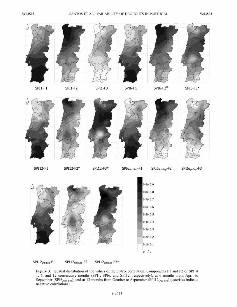
Figure 3. Spatial distribution of the values of the matrix correlation. Components F1 and F2 of SPI at1, 6, and 12 consecutive months (SPI1, SPI6, and SPI12, respectively); at 6 months from April toSeptember (SPI6Apr-Sep); and at 12 months from October to September (SPI12Oct-Sep) (asterisks indicatenegative correlations).
6 of 13
W03503 SANTOS ET AL.: VARIABILITY OF DROUGHTS IN PORTUGAL W03503
with the original series in the case of SPI6, SPI12, andSPI12Oct-Sep.[35] The previous results indicated that with the three
main components F1, F2, and F3 a spatial classification isachieved, with two well-defined regions, one located in thenorth and the other in the south of Portugal and with anintermediate region that promotes the transition from thewet north to the arid and semiarid south. The spatialclassification was similar for all the time scales used.[36] It should be stressed that from a hydrological point
of view the two previous regions are quite different: thenorth and especially the northwestern region has much morewater along with a very regular regime; toward south, thewater availability decreases progressively (as denoted byFigure 1) and the regime becomes more and more irregularwith more than 75% of the precipitation occurring during afew months of the wet semester.
3.2. Nonhierarchical Cluster Analysis: SpatialVariability of Droughts
[37] For all the SPI series (SPI1, SPI6, SPI12, SPI6Apr-Sep,and SPI12Oct-Sep), the spatial grouping obtained with thecluster analysis was similar to the one given by the PCA.For example, Figure 4 shows the spatial distribution of theclusters formed with the SPI6Apr-Sep series considering two,three, and four classification groups.[38] To evaluate the appropriateness of the classifications,
the Euclidean distances between clusters were examined.
These distances for the clusters analysis with two, three, andfour groups are shown in Table 2 for the SPI6Apr-Sep series.These results show that the best grouping is with threeclusters.[39] Note that clusters 1 (southern rain gages) and 2
(northern rain gages) were relatively more close (Euclideandistance = 0.67) in the classification with two groups incomparison with clusters 1 (northern rain gages) and 3(southern rain gages) (Euclidean distance = 0.88) in theclassification with three groups. So, three different regionsthat are well-defined spatially (north, central, and southregions) can be considered (Figure 4b). Despite the fact that,compared to the PCA, there is a central region clearlydelimited (Cluster 2), the spatial classification that resultedfrom the cluster analysis is similar to the one obtained withthe PCA method (Figure 3), which suggests that bothmethods can be used to identify spatial areas with differenttemporal patterns.[40] The classification with four groups was rejected
because the clusters 2 and 3 (northern rain gages)(Figure 4c), which conform approximately the cluster 1on the analysis with three groups (Figure 4b), presentedEuclidean distances more close to the cluster 4 (southernrain gages) of the analysis with four groups in comparisonwith the classification with three groups (Table 2). So, inFigure 4c the Euclidean distances between cluster 2 (northernrain gages) and 4 (southern rain gages) was 0.72 andbetween 3 (northern rain gages) and 4 (southern rain gages)
Figure 4. SPI6Apr-Sep series. Comparison of clusters analysis with (a) two, (b) three, and (c) fourclassification groups.
W03503 SANTOS ET AL.: VARIABILITY OF DROUGHTS IN PORTUGAL
7 of 13
W03503
was 0.14, while in Figure 4b the Euclidean distance betweencluster 1 (northern rain gages) and 3 (southern rain gages)was 0.88.
3.3. Temporal Pattern and Areal Evolutionof Droughts
[41] The seasonal SPI6Apr-Sep series were chosen for thisanalysis as they reflect the driest period in Portugal, fromthe middle of spring to the end of summer, when droughtsare most critical as they affect the agriculture sector which isin Portugal the foremost water consuming sector. Also, thespatial classification that resulted from the PCA, Figure 3,showed that both subannual (SPI1, SPI6, and SPI12) orinterannual (SPI6Apr-Sep, SPI12Oct-Sep) time scales of SPI ledto similar patterns which makes valid to continue theanalysis based on one of those scales.[42] The temporal evolution of the components F1 and F2
of the PCA and of cluster 3 and 1 for three classificationgroups is shown in Figure 5. Figure 5 shows that the
southern part of Portugal (component F1 and cluster 3)suffered several extreme droughts, starting in the beginningof the 1920s, mid 1930s, 1940s, 1950s, and mid 1970s.Some of those droughts were particularly severe as theywere prolonged in time such as the one in the mid 1950s. Inthe northwestern part of Portugal (component F2 andcluster 1), although fewer drought events were detected,two extreme droughts are quite clear: one in the mid 1930sand the other in the beginning of the 1990s. The firstepisode was short and the second one more prolonged intime.[43] The results for each area, when comparing both
methods (PCA and cluster analysis), are quite similar. Infact the Pearson correlation coefficient between PCA-F1and cluster 3 was 0.964 and between PCA-F2 and cluster 1was 0.938, with these high values clearly expressing theproximity of the results.[44] The differences between the northwestern and south-
ern areas can be related with the water availability andtemporal variability, the former region having more waterand a regular hydrologic regime, as previously mentioned.[45] According to PCA and once more for SPI6Apr-Sep,
Figure 6 shows the areas of Figure 3 with correlationshigher than 0.7. For each one of those areas the percentagesof area affected by moderate, severe, and extreme drought(according to the SPI categories of Table 1) were computed.For that purpose an influence area was assign to each raingage by applying the Thiessen polygon method [Vicente-Serrano et al., 2004] using Arcgis 9.3. The area attributed toa specified drought category was given by the cumulativeareas of the rain gages with values of SPI6Apr-Sep within thelimits that define such drought category. The resultsachieved are presented in Figure 7.[46] Figure 7 shows that in general terms, the southern
part of Portugal (F1) is more affected by drought eventsthan the northwestern part (F2). From 1910 to 2004 the
Table 2. SPI6Apr-Sep Seriesa
Cluster 1 Cluster 2 Cluster 3 Cluster 4
Two Classification GroupsCluster 1 0 0.449914Cluster 2 0.670756 0
Three Classification GroupsCluster 1 0 0.221728 0.778282Cluster 2 0.470880 0 0.351966Cluster 3 0.882203 0.593267 0
Four Classification GroupsCluster 1 0 0.207486 0.655584 0.934866Cluster 2 0.455507 0 0.289587 0.524088Cluster 3 0.809681 0.538133 0 0.019968Cluster 4 0.966885 0.723939 0.141311 0
aEuclidean distances between clusters for analysis with two, three andfour classification groups (distances below diagonal and squared distancesabove diagonal).
Figure 5. Temporal evolution of components F1 and F2 of the PCA analysis for data series SPI6Apr-Sepand means of each cluster for analysis with three classification groups.
8 of 13
W03503 SANTOS ET AL.: VARIABILITY OF DROUGHTS IN PORTUGAL W03503
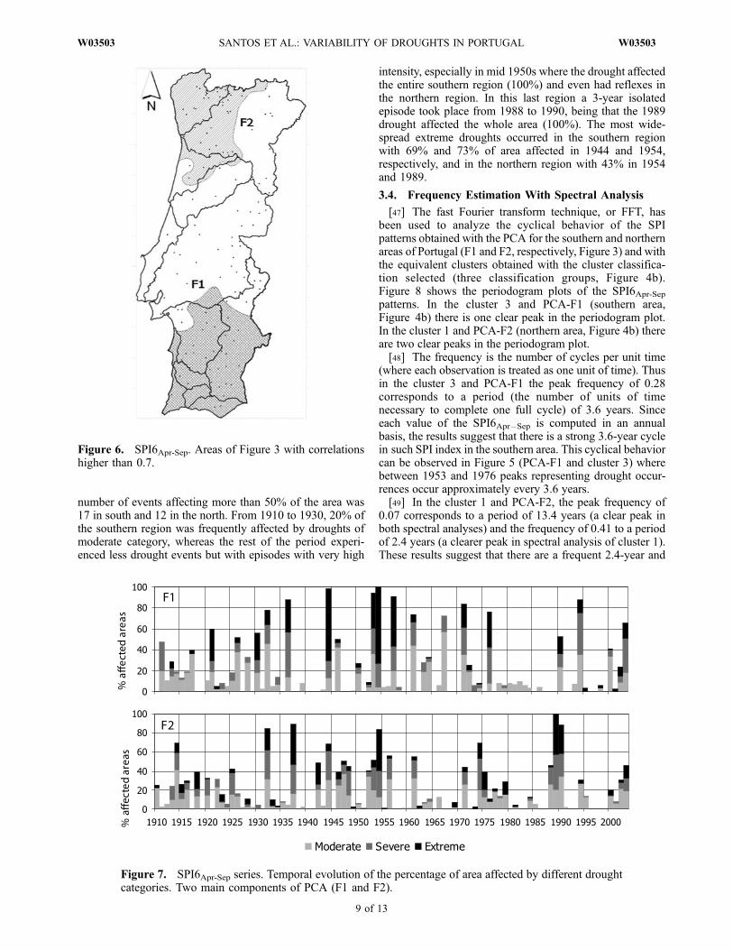
number of events affecting more than 50% of the area was17 in south and 12 in the north. From 1910 to 1930, 20% ofthe southern region was frequently affected by droughts ofmoderate category, whereas the rest of the period experi-enced less drought events but with episodes with very high
intensity, especially in mid 1950s where the drought affectedthe entire southern region (100%) and even had reflexes inthe northern region. In this last region a 3-year isolatedepisode took place from 1988 to 1990, being that the 1989drought affected the whole area (100%). The most wide-spread extreme droughts occurred in the southern regionwith 69% and 73% of area affected in 1944 and 1954,respectively, and in the northern region with 43% in 1954and 1989.
3.4. Frequency Estimation With Spectral Analysis
[47] The fast Fourier transform technique, or FFT, hasbeen used to analyze the cyclical behavior of the SPIpatterns obtained with the PCA for the southern and northernareas of Portugal (F1 and F2, respectively, Figure 3) and withthe equivalent clusters obtained with the cluster classifica-tion selected (three classification groups, Figure 4b).Figure 8 shows the periodogram plots of the SPI6Apr-Seppatterns. In the cluster 3 and PCA-F1 (southern area,Figure 4b) there is one clear peak in the periodogram plot.In the cluster 1 and PCA-F2 (northern area, Figure 4b) thereare two clear peaks in the periodogram plot.[48] The frequency is the number of cycles per unit time
(where each observation is treated as one unit of time). Thusin the cluster 3 and PCA-F1 the peak frequency of 0.28corresponds to a period (the number of units of timenecessary to complete one full cycle) of 3.6 years. Sinceeach value of the SPI6Apr–Sep is computed in an annualbasis, the results suggest that there is a strong 3.6-year cyclein such SPI index in the southern area. This cyclical behaviorcan be observed in Figure 5 (PCA-F1 and cluster 3) wherebetween 1953 and 1976 peaks representing drought occur-rences occur approximately every 3.6 years.[49] In the cluster 1 and PCA-F2, the peak frequency of
0.07 corresponds to a period of 13.4 years (a clear peak inboth spectral analyses) and the frequency of 0.41 to a periodof 2.4 years (a clearer peak in spectral analysis of cluster 1).These results suggest that there are a frequent 2.4-year and
Figure 6. SPI6Apr-Sep. Areas of Figure 3 with correlationshigher than 0.7.
Figure 7. SPI6Apr-Sep series. Temporal evolution of the percentage of area affected by different droughtcategories. Two main components of PCA (F1 and F2).
W03503 SANTOS ET AL.: VARIABILITY OF DROUGHTS IN PORTUGAL
9 of 13
W03503
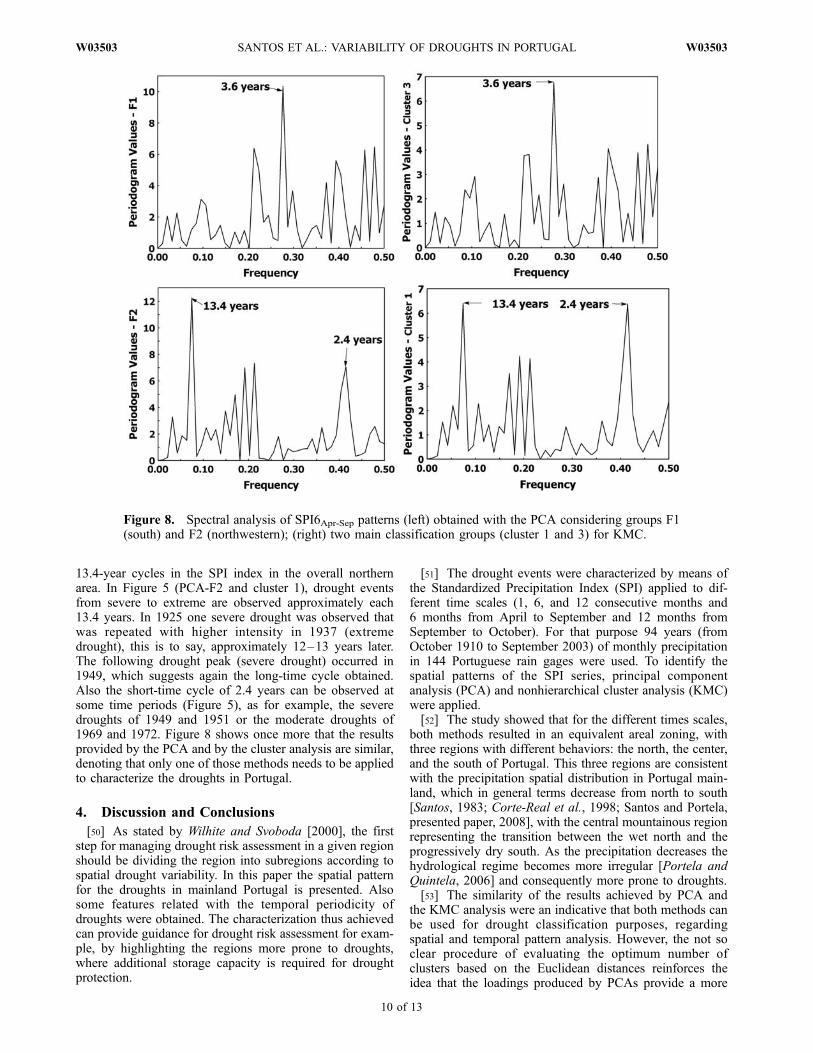
13.4-year cycles in the SPI index in the overall northernarea. In Figure 5 (PCA-F2 and cluster 1), drought eventsfrom severe to extreme are observed approximately each13.4 years. In 1925 one severe drought was observed thatwas repeated with higher intensity in 1937 (extremedrought), this is to say, approximately 12–13 years later.The following drought peak (severe drought) occurred in1949, which suggests again the long-time cycle obtained.Also the short-time cycle of 2.4 years can be observed atsome time periods (Figure 5), as for example, the severedroughts of 1949 and 1951 or the moderate droughts of1969 and 1972. Figure 8 shows once more that the resultsprovided by the PCA and by the cluster analysis are similar,denoting that only one of those methods needs to be appliedto characterize the droughts in Portugal.
4. Discussion and Conclusions
[50] As stated by Wilhite and Svoboda [2000], the firststep for managing drought risk assessment in a given regionshould be dividing the region into subregions according tospatial drought variability. In this paper the spatial patternfor the droughts in mainland Portugal is presented. Alsosome features related with the temporal periodicity ofdroughts were obtained. The characterization thus achievedcan provide guidance for drought risk assessment for exam-ple, by highlighting the regions more prone to droughts,where additional storage capacity is required for droughtprotection.
[51] The drought events were characterized by means ofthe Standardized Precipitation Index (SPI) applied to dif-ferent time scales (1, 6, and 12 consecutive months and6 months from April to September and 12 months fromSeptember to October). For that purpose 94 years (fromOctober 1910 to September 2003) of monthly precipitationin 144 Portuguese rain gages were used. To identify thespatial patterns of the SPI series, principal componentanalysis (PCA) and nonhierarchical cluster analysis (KMC)were applied.[52] The study showed that for the different times scales,
both methods resulted in an equivalent areal zoning, withthree regions with different behaviors: the north, the center,and the south of Portugal. This three regions are consistentwith the precipitation spatial distribution in Portugal main-land, which in general terms decrease from north to south[Santos, 1983; Corte-Real et al., 1998; Santos and Portela,presented paper, 2008], with the central mountainous regionrepresenting the transition between the wet north and theprogressively dry south. As the precipitation decreases thehydrological regime becomes more irregular [Portela andQuintela, 2006] and consequently more prone to droughts.[53] The similarity of the results achieved by PCA and
the KMC analysis were an indicative that both methods canbe used for drought classification purposes, regardingspatial and temporal pattern analysis. However, the not soclear procedure of evaluating the optimum number ofclusters based on the Euclidean distances reinforces theidea that the loadings produced by PCAs provide a more
Figure 8. Spectral analysis of SPI6Apr-Sep patterns (left) obtained with the PCA considering groups F1(south) and F2 (northwestern); (right) two main classification groups (cluster 1 and 3) for KMC.
10 of 13
W03503 SANTOS ET AL.: VARIABILITY OF DROUGHTS IN PORTUGAL W03503
clear and simple method to recognize distinct temporalpatterns.[54] Previous studies have shown that during positive
phases of the North Atlantic Oscillation (NAO), negativeSPI averages (indicative of drought conditions) are recordedin southern Europe, whereas the opposite trends occurduring negative phases [Trigo et al., 2002; Lopez-Morenoand Vicente-Serrano, 2008]. In general, this trend isobserved in the SPI patterns obtained in this study. Accord-ing to Lopez-Moreno and Vicente-Serrano [2008], forexample, the years 1920, 1957, 1961, and 1990 wereidentified as having positive phases of the NAO and inour work these years have showed strong negative SPIvalues when short, medium, and long time scales (1, 6, and12 months) were considered.[55] Spectral analysis (energy versus frequency) was
particularly useful to detect periodical signals in the SPItime series patterns. The spectral analysis derived from thePCA and the KMC results by applying fast FourierTransform algorithm were equivalent denoting more fre-quent cycles of dry events in the southern region (droughtsfrom moderate to extreme approximately every 3.6 years)than in the northern region (droughts from severe to extremeapproximately every 13.4 years). The drought short-timeperiodicity observed in the southern region might be asso-ciated with the immediate and significant influence of theNorth Atlantic Oscillation (NAO) on the precipitationregimes in the Atlantic and Mediterranean sectors [Lopez-Moreno et al., 2007; Lopez-Moreno and Vicente-Serrano,2008; Kucuk et al., 2009]. Thus Polonskii et al. [2004] andKucuk et al. [2009] found that the spectra of the NAO indexcontain significant peaks corresponding to periods of 2–4and 6–10 years. However, explaining relations between theNAO and the periodicity of more than 10 years, detected inthe northern region, remains a challenging task that shouldinclude the study of the interaction of other regionalphenomenons such as the soil moisture oscillation [Simset al., 2002; Abbot and Emanuel, 2007].[56] It may be noted that the conclusions of the spectral
analysis need to be reinforced through the research of theprocess of energy variations in terms of when the droughtevents occur (energy versus time frequency) which could bedeveloped in future works using the wavelet transformanalysis [Kucuk et al., 2009]. Thus inferences related withthe connection among frequency peaks and effective cycledrought patterns in the data and with the translation ofsuch drought cycles into occurrence probabilities could beobtained. Likewise, additional research needs to be carriedregarding the physical mechanisms that explain the resultsachieved in connection to other local factors, such as theparameters that control temporal changes in the influence ofthe NAO phases on Portugal droughts or the analysis of otherglobal teleconnection patterns (ENSO and east Atlantic-westRussia, EAWR).
[57] Acknowledgment. The authors gratefully acknowledge theAndalusian government for providing financing through the project08.44103.82A.008 (Junta de Andalucıa, Spain, ‘‘Accion Exterior’’).
ReferencesAbbot, D. S., and K. A. Emanuel (2007), A tropical and subtropical land-sea-atmosphere drought oscillation mechanism, J. Atmos. Sci., 64,4458–4466, doi:10.1175/2007JAS2186.1.
Agnew, C. T. (2000), Using the SPI to identify drought, Drought NetworkNews, 12, 6–12.
Bates, B. C., Z. W. Kundzewicz, S. Wu, and J. P. Palutikof (Eds.) (2008),Climate Change and Water, Tech. Pap. VI, 210 pp., IntergovernmentalPanel on Clim. Change, Geneva, Switzerland.
Bloomfield, P. (Ed.) (1976), Fourier Analysis of Time Series: An Introduc-tion, 272 pp., John Wiley, New York.
Bonaccorso, B., I. Bordi, A. Cancelliere, G. Rossi, and A. Sutera (2003),Spatial variability of drought: An analysis of the SPI in Sicily, WaterResour. Manage., 17, 273–296, doi:10.1023/A:1024716530289.
Bordi, I., and A. Sutera (2001), Fifty years of precipitation: Some spatiallyremote teleconnections, Water Resour. Manage., 15, 247 – 280,doi:10.1023/A:1013353822381.
Bordi, I., F. W. Fraedrich, F. W. Gerstengarbe, C. Werner, and A. Sutera(2004), Spatio-temporal variability of dry and wet periods in easternChina, Theor. Appl. Climatol., 77, 125–138, doi:10.1007/s00704-003-0029-0.
Corte-Real, J., B. Qian, and H. Xu (1998), Regional climate change inPortugal: Precipitation variability associated with large-scale atmosphericcirculation, Int. J. Climatol., 18, 619–635, doi:10.1002/(SICI)1097-0088(199805)18:6<619::AID-JOC271>3.0.CO;2-T.
Daniel, W. W. (Ed.) (1990), Applied Nonparametric Statistics, 2nd ed.,656 pp., Wadsworth, Boston, Mass.
DeGaetano, A. T. (1996), Delineation of mesoscale climate zones in thenortheastern United States using a novel approach to cluster analysis,J. Clim., 9, 1765 – 1782, doi:10.1175/1520-0442(1996)009<1765:DOMCZI>2.0.CO;2.
Domingos, S. I. (2006), Analise do ındice de seca Standardized PrecipitationIndex (SPI) em Portugal Continental e sua comparacao com o PalmerDrought Severity Index (PDSI), M.S. thesis, Univ. de Lisboa, Lisbon,Portugal.
Edwards, D. C., and T. B. McKee (1997), Characteristics of 20th centurydrought in the United States at multiple time scales, Atmos. Sci. Pap. 634,Colorado State Univ., Fort Collins.
Esteban, P., P. D. Jones, J. Martyn-Vide, and M. Mases (2005), Atmo-spheric circulation patterns related to heavy snowfall days in Andorra,Pyrenees, Int. J. Climatol., 25, 319–329, doi:10.1002/joc.1103.
Fleming, S. W., A. M. Lavenue, A. H. Aly, and A. Adams (2002), Practicalapplications of spectral analysis to hydrologic time series, Hydrol. Pro-cess., 16, 565–574, doi:10.1002/hyp.523.
Gong, X., and M. B. Richman (1995), On the application of cluster analysisto growing season precipitation data in North America east of theRockies, J. Clim., 8, 897 –931, doi:10.1175/1520-0442(1995)008<0897:OTAOCA>2.0.CO;2.
Gutierrez-Estrada, J. C., and I. Pulido-Calvo (2007), Water temperatureregimen analysis of intensive fishfarms associated with cooling efflu-ents from power plants, Biosystems Eng., 96(4), 581–591, doi:10.1016/j.biosystemseng.2007.01.006.
Guttman, N. B. (1998), Comparing the Palmer drought index and theStandardized Precipitation Index, J. Am. Water Resour. Assoc., 34,113–121, doi:10.1111/j.1752-1688.1998.tb05964.x.
Guttman, N. B. (1999), Accepting the standardized precipitation index: Acalculation algorithm, J. Am. Water Resour. Assoc., 35, 311–322,doi:10.1111/j.1752-1688.1999.tb03592.x.
Hair, J. F., R. E. Anderson, R. L. Tatham, B. Babin, and B. Black (Eds.)(2005), Multivariate Data Analysis, 6th ed., 928 pp., Prentice-Hall,London.
Hayes, M., D. A. Wilhite, M. Svodoba, and O. Vanyarkho (1999),Monitoring the 1996 drought using the standardized precipitation index,Bull. Am. Meteorol. Soc., 80, 429–438, doi:10.1175/1520-0477(1999)080<0429:MTDUTS>2.0.CO;2.
Henriques, A. G., and M. J. J. Santos (1999), Regional drought distributionmodel, Phys. Chem. Earth, Part B, 24(1/2), 19–22.
Hisdal, H., and L. M. Tallaksen (2003), Estimation of regional meteorolo-gical and hydrological drought characteristics: A case study for Denmark,J. Hydrol., 281, 230–247, doi:10.1016/S0022-1694(03)00233-6.
Jolliffe, I. T. (Ed.) (2002), Principal Component Analysis, 2nd ed., 502 pp.,Springer, New York.
Kahya, E., M. C. Demirel, and O. A. Beg (2008a), Hydrologic homoge-neous regions using monthly streamflow in Turkey, Earth Sci. Res. J.,12(2), 181–193.
Kahya, E., S. Kalayc, and T. C. Piechota (2008b), Streamflow regionaliza-tion: Case study of Turkey, J. Hydrol. Eng., 13(4), 205 – 214,doi:10.1061/(ASCE)1084-0699(2008)13:4(205).
Kalayci, S., and E. Kahya (2006), Assessment of streamflow variabilitymodes in Turkey: 1964 – 1994, J. Hydrol., 324(1 – 4), 163 – 177,doi:10.1016/j.jhydrol.2005.10.002.
W03503 SANTOS ET AL.: VARIABILITY OF DROUGHTS IN PORTUGAL
11 of 13
W03503
Karl, T. R., and A. J. Koscielny (1982), Drought in the United States:1895–1981, J. Climatol., 2, 313–329, doi:10.1002/joc.3370020402.
Klugman, M. R. (1978), Drought in the upper midwest, 1931–1969,J. Appl. Meteorol., 17, 1425–1431, doi:10.1175/1520-0450(1978)017<1425:DITUM>2.0.CO;2.
Komuscu, A. U. (1999), Using the SPI to analyse spatial and temporalpatterns of drought in Turkey, Drought Network News, 11, 7–13.
Kucuk, M., E. Kahya, T. M. Cengiz, and M. Karaca (2009), North AtlanticOscillation influences on Turkish lake levels, Hydrol. Process., 23, 893–906, doi:10.1002/hyp.7225.
Lins, H. F. (1985), Interannual streamflow variability in the United Statesbased on principal components, Water Resour. Res., 21(5), 691–701,doi:10.1029/WR021i005p00691.
Lloyd-Hughes, B., and M. A. Saunders (2002), Seasonal prediction ofEuropean spring precipitation from El Nino–Southern Oscillation andlocal sea-surface temperatures, Int. J. Climatol., 22, 1–14, doi:10.1002/joc.723.
Lo, K. M., C. S. Chen, J. T. Clayton, and D. D. Adrian (1975), Simulationof temperature and moisture changes in wheat storage due to weathervariability, J. Agric. Eng. Res., 20(1), 47 – 53, doi:10.1016/0021-8634(75)90094-3.
Lopez-Bermudez, F., and M. C. Sanchez (1997), Las sequıas y su impactoen el riesgo de desertificacion de la cuenca del Segura: Apuntes para lagestion y sostenibilidad del agua, Rev. Cienc. Soc., 17, 155–168.
Lopez-Moreno, J. I., and S. M. Vicente-Serrano (2008), Positive and nega-tive phases of the wintertime North Atlantic Oscillation and droughtoccurrence over Europe: A multi-temporal-scale approach, J. Clim., 21,1220–1243, doi:10.1175/2007JCLI1739.1.
Lopez-Moreno, J. I., S. Beguerıa, S. M. Vicente-Serrano, and J. M. Garcıa-Ruiz (2007), Influence of the North Atlantic Oscillation on waterresources in central Iberia: Precipitation, streamflow anomalies, andreservoir management strategies, Water Resour. Res., 43, W09411,doi:10.1029/2007WR005864.
Lopez-Moreno, J. I., S. M. Vicente-Serrano, S. Beguerıa, J. M. Garcıa-Ruiz,M. M. Portela, and A. B. Almeida (2009), Dam effects on droughtsmagnitude and duration in a transboundary basin: The Lower River Tagus,Spain and Portugal, Water Resour. Res., 45, W02405, doi:10.1029/2008WR007198.
Loukas, A., and L. Vasiliades (2004), Probabilistic analysis of droughtspatiotemporal characteristics in Thessaly region, Greece, Nat. HazardsEarth Syst. Sci., 4, 719–731.
Moreira, E. E., A. A. Paulo, L. S. Pereira, and J. T. Mexia (2006), Analysisof SPI drought class transitions using loglinear models, J. Hydrol., 331,349–359, doi:10.1016/j.jhydrol.2006.05.022.
New, M., M. Todd, M. Hulme, and P. Jones (2002), Precipitation measure-ments and trends in the twentieth century, Int. J. Climatol., 21, 1899–1922.
Ntale, H. K., and T. Gan (2003), Drought indices and their application toEast Africa, Int. J. Climatol., 23, 1335–1357, doi:10.1002/joc.931.
Oliver, M. A., and R. Webster (1990), Kriging: A method of interpolationfor geographical information system, Int. J. Geogr. Inf. Syst., 4(3), 313–332, doi:10.1080/02693799008941549.
Park, H. H. (1998), Analysis and prediction of walleye Pollock (Theragrachalcogramma) landings in Korea by time series analysis, Fish. Res., 38,1–7, doi:10.1016/S0165-7836(98)00118-0.
Pasquini, A., K. L. Lecomte, E. L. Piovano, and P. J. Depetris (2006),Recent rainfall and runoff variability in central Argentina, Quat. Int.,158, 127–139, doi:10.1016/j.quaint.2006.05.021.
Paulo, A. A., and L. S. Pereira (2006), Drought concepts and characteriza-tion, Comparing drought indices applied at local and regional scales,Water Int., 31(1), 37–49, doi:10.1080/02508060608691913.
Paulo, A. A., and L. S. Pereira (2007), Prediction of SPI drought classtransitions using Markov chains, Water Resour. Manage., 21(10),1813–1827, doi:10.1007/s11269-006-9129-9.
Paulo, A. A., and L. S. Pereira (2008), Stochastic prediction of droughtclass transitions, Water Resour. Manage., 22(9), 1277 – 1296,doi:10.1007/s11269-007-9225-5.
Paulo, A. A., L. S. Pereira, and P. G. Matias (2003), Analysis of local andregional droughts in southern Portugal using the theory of runs and theStandardised Precipitation Index, in Tools for Drought Mitigation inMediterranean Regions, edited by G. Rossi et al., pp. 55–78, Springer,New York.
Pires, V. C. (2003), Frequencia e intensidade de fenomenos meteorologicosextremos associados a precipitacao, Desenvolvimento de um sistema demonitorizacao de situacoes de seca em Portugal Continental, M.S. thesis,Univ. de Lisboa, Lisbon, Portugal.
Polonskii, A. B., D. V. Basharin, E. N. Voskresenskaya, and S. Worley(2004), North Atlantic Oscillation: Description, mechanisms, and influ-ence on the Eurasian climate, Phys. Oceanogr., 14(2), 96 – 113,doi:10.1023/B:POCE.0000037873.85289.6e.
Portela, M. M., and A. C. Quintela (2006), Estimacao em Portugal Con-tinental de escoamento e de capacidades uteis de albufeiras de regular-izacao na ausencia de informacao (in Portuguese), Recursos Hidrıcos,27(2), 7–18.
Pulido-Calvo, I., J. C. Gutierrez-Estrada, J. Roldan, and R. Lopez-Luque(2006), Regulating reservoirs in pressurized irrigation water supply sys-tems, J. Water Supply, 55(5), 367–381.
Rasilla, D. (2002), Aplicacion de un metodo de clasificacion sinoptica a laPenınsula Iberica, Invest. Geogr., 30, 27–45.
Rencher, A. C. (Ed.) (1998),Multivariate Statistical Inference and Applica-tions, John Wiley, New York.
Rhee, J., J. Im, G. J. Carbone, and J. R. Jensen (2008), Delineation ofclimate regions using in-situ and remotely sensed data for the Carolinas,Remote Sens. Environ., 112, 3099–3111, doi:10.1016/j.rse.2008.03.001.
Richman, M. B. (1986), Rotation of principal components, J. Climatol., 6,29–35.
Romero, R., G. Summer, C. Ramis, and A. Genoves (1999), A classuifica-tion of the atmospheric circulation patterns producing significant dailyprecipitation in the Spanish Mediterranean area, Int. J. Climatol., 19,765 – 785, doi:10.1002/(SICI)1097-0088(19990615)19:7<765::AID-JOC388>3.0.CO;2-T.
Sankarasubramanian, A., and K. Srinivasan (1999), Investigation and com-parison of sampling properties of L-moments and conventional moments,J. Hydrol., 218, 13–34, doi:10.1016/S0022-1694(99)00018-9.
Santos, M. A. (1983), Regional droughts: A stochastic characterization,J. Hydrol., 66, 183–211, doi:10.1016/0022-1694(83)90185-3.
Santos, F. D., and P. M. Miranda (Eds.) (2008), Alteracoes Climaticas emPortugal. Cenarios, Impactos e Medidas de Adaptacao, Projecto SIAM,Gradiva, Lisbon, Portugal.
Santos, M. J. J., R. Verıssimo, and R. Rodrigues (2001), Hydrologicaldrought computation and its comparison with meteorological drought,in ARIDE—Assessment of the Regional Impact of Droughts in Europe,Final Report EU, edited by S. Demuth and K. Stahl, pp. 78–79, Inst. ofHydrol., Freiburg, Germany.
Seiler, R. A., M. Hayes, and L. Bressan (2002), Using the StandardizedPrecipitation Index for flood risk monitoring, Int. J. Climatol., 22, 1365–1376, doi:10.1002/joc.799.
Shukla, S., S. Mostaghimi, and M. Al-Smadi (2000), Multivariate techniquefor baseflow separation using water quality data, J. Hydrol. Eng., 5(2),172–179, doi:10.1061/(ASCE)1084-0699(2000)5:2(172).
Sims, A. P., D. S. Nigoyi, and S. Raman (2002), Adopting indices forestimating soil moisture: A North Carolina case study, Geophys. Res.Lett., 29(8), 1183, doi:10.1029/2001GL013343.
Singh, P. K., V. Kumar, R. C. Purohit, M. Kothari, and P. K. Dashora(2009), Application of principal component analysis in grouping geo-morphic parameters for hydrologic modeling, Water Resour. Manage.,23, 325–339, doi:10.1007/s11269-008-9277-1.
Smith, L. I. (Ed.) (2002), A Tutorial on Principal Components Analysis,Computer Sciences, vol. 26, Univ. of Otago, Dunedin, New Zealand.
Stahl, K., and S. Demuth (Eds.) (1999), Methods for regional classificationof streamflow drought series: Cluster analysis, technical report to theAride Project, Inst. of Hydrol., Univ. of Freiburg, Freiburg im Breisgau,Germany.
Stooksbury, D. E., and P. J. Michaels (1991), Cluster analysis of South-eastern U.S. climate stations, Theor. Appl. Climatol., 44, 143–150,doi:10.1007/BF00868169.
Tipping, M. E., and C. M. Bishop (1999), Probabilistic principal componentanalysis, J. R. Stat. Soc., Ser. B, 61(3), 611–622, doi:10.1111/1467-9868.00196.
Trigo, R. M., T. J. Osborn, and J. M. Corte-Real (2002), The North AtlanticOscillation influence on Europe: Climate impacts and associated physicalmechanisms, Clim. Res., 20, 9–17.
Vicente-Serrano, S. M. (2005), Las Sequıas Climaticas en el Valle Mediodel Ebro: Factores Atmosfericos, Evolucion Temporal y VariabilidadEspacial, Ser. Invest., vol. 49, Publ. Cons. de Prot. de la Nat. de Aragon,Zaragoza, Spain.
Vicente-Serrano, S. M. (2006a), Spatial and temporal analysis of droughtsin the Iberian Peninsula (1910–2000), Hydrol. Sci. J., 51(1), 83–97,doi:10.1623/hysj.51.1.83.
Vicente-Serrano, S. M. (2006b), Differences in spatial patterns of droughton different time scales: An analysis of the Iberian Peninsula, WaterResour. Manage., 20, 37–60, doi:10.1007/s11269-006-2974-8.
12 of 13
W03503 SANTOS ET AL.: VARIABILITY OF DROUGHTS IN PORTUGAL W03503
Vicente-Serrano, S. M., and J. I. Lopez-Moreno (2005), Hydrologicalresponse to different time scales of climatological drought: An evaluationof the standardized precipitation index in a mountainous Mediterraneanbasin, Hydrol. Earth Syst. Sci., 9, 523–533.
Vicente-Serrano, S. M., J. S. Gonzalez-Hidalgo, M. Luis, and J. Raventos(2004), Drought patterns in the Mediterranean area: The Valencia region(eastern Spain), Clim. Res., 26, 5–15, doi:10.3354/cr026005.
Webster, R., and M. A. Oliver (1990), Numerical classification: Non-hierarchical methods, in Statistical Methods in Soil and Land ResourceSurvey, chap. 11, pp. 191–212, Oxford Univ. Press, Oxford, U. K.
Wilhite, D. A., and M. D. Svoboda (2000), Drought early warning systemsin the context of drought preparedness and mitigation, in Early WarningSystems for Drought Preparedness and Drought Management, edited byD. A. Wilhite, M. V. K. Sivakumar, and D. A. Woods, pp. 1–21, WorldMeteorol. Org., Lisbon, Portugal.
Yamoah, C. F., D. F. Walters, C. A. Shapiro, C. A. Francis, and M. J. Hayes(2000), Standardized precipitation index and nitrogen rate effects on cropyields and risk distribution in maize, Agric. Ecosyst. Environ., 80, 113–120, doi:10.1016/S0167-8809(00)00140-7.
����������������������������M. M. Portela, Departamento Engenharia Civil, SHRH, Instituto
Superior Tecnico, Avenida Rovisco Pais, P-1049-001 Lisboa, Portugal.([email protected])
I. Pulido-Calvo, Departamento Ciencias Agroforestales, EPS, CampusUniversitario de La Rabida, Universidad de Huelva, E-21819 Palos de laFrontera, Spain. ([email protected])
J. F. Santos, Departamento Engenharia, ESTIG, Instituto Politecnico deBeja, Rua Afonso III, P-7800-050 Beja, Portugal. ([email protected])
W03503 SANTOS ET AL.: VARIABILITY OF DROUGHTS IN PORTUGAL
13 of 13
W03503