Classiﬂcation with Incomplete Data Using Dirichlet Process...

Classification with Incomplete DataUsing Dirichlet Process Priors

Chunping Wang [email protected] Liao [email protected] Carin [email protected] of Electrical and Computer EngineeringDuke UniversityDurham, NC 27708-0291, USA

David B. Dunson [email protected]

Department of Statistical ScienceDuke UniversityDurham, NC 27708-0291, USA

Abstract

A non-parametric hierarchical Bayesian framework is developed for designing a classifier,based on a mixture of simple (linear) classifiers. Each simple classifier is termed a local“expert”, and the number of experts and their construction are manifested via a Dirichletprocess formulation. The simple form of the “experts” allows analytical handling of incom-plete data. The model is extended to allow simultaneous design of classifiers on multipledata sets, termed multi-task learning, with this also performed non-parametrically via theDirichlet process. Fast inference is performed using variational Bayesian (VB) analysis, andexample results are presented for several data sets. We also perform inference via Gibbssampling, to which we compare the VB results.

Keywords: Classification, Incomplete Data, Expert, Dirichlet process, Variational Bayesian,Multi-task Learning

1. Introduction

In many applications one must deal with data that have been collected incompletely. Forexample, in censuses and surveys, some participants may not respond to certain questions(Rubin, 1987); in email spam filtering, server information may be unavailable for emails fromexternal sources (Dick et al., 2008); in medical studies, measurements on some subjects maybe partially lost at certain stages of the treatment (Ibrahim, 1990); in DNA analysis, gene-expression microarrays may be incomplete due to insufficient resolution, image corruption,or simply dust or scratches on the slide (Wang et al., 2006); in sensing applications, asubset of sensors may be absent or fail to operate at certain regions (Williams and Carin,2005). Unlike in semi-supervised learning (Ando and Zhang, 2005) where missing labels(responses) must be addressed, features (inputs) are partially missing in the aforementionedincomplete-data problems. Since most data analysis procedures (for example, regression andclassification) are designed for complete data, and cannot be directly applied to incompletedata, the appropriate handling of missing data is challenging.

1

Traditionally, data are often “completed” by ad hoc editing, such as case deletion andsingle imputation, where feature vectors with missing values are simply discarded or com-pleted with specific values in the initial stage of analysis, before the main inference (forexample, mean imputation and regression imputation (see Schafer and Graham, 2002)).Although analysis procedures designed for complete data become applicable after these ed-its, shortcomings are clear. For case deletion, discarding information is generally inefficient,especially when data are scarce. Secondly, the remaining complete data may be statisticallyunrepresentative. More importantly, even if the incomplete-data problem is eliminated byignoring data with missing features in the training phase, it is still inevitable in the teststage since test data cannot be ignored simply because a portion of features are missing.For single imputation, the main concern is that the uncertainty of the missing features isignored by imputing fixed values.

The work of Rubin (1976) developed a theoretical framework for incomplete-data prob-lems, where widely-cited terminology for missing patterns was first defined. It was proventhat ignoring the missing mechanism is appropriate (Rubin, 1976) under the missing at ran-dom (MAR) assumption, meaning that the missing mechanism is conditionally independentof the missing features given the observed data. As elaborated later, given the MAR as-sumption (Dick et al., 2008; Ibrahim, 1990; Williams and Carin, 2005), incomplete datacan generally be handled by full maximum likelihood and Bayesian approaches; however,when the missing mechanism does depend on the missing values (missing not at randomor MNAR), a problem-specific model is necessary to describe the missing mechanism, andno general approach exists. In this paper, we address missing features under the MARassumption. Previous work in this setting may be placed into two groups, depending onwhether the missing data are handled before algorithm learning or within the algorithm.

For the former, an extra step is required to estimate p(xm|xo), conditional distributionsof missing values given observed ones, with this step distinct from the main inference al-gorithm. After p(xm|xo) is learned, various imputation methods may be performed. As aMonte Carlo approach, Bayesian multiple imputation (MI) (Rubin, 1987) is widely used,where multiple (M > 1) samples from p(xm|xo) are imputed to form M “complete” datasets, with the complete-data algorithm applied on each, and results of those imputed datasets combined to yield a final result. The MI method “completes” data sets so that algo-rithms designed for complete data become applicable. Furthermore, Rubin (1987) showedthat MI does not require as many samples as Monte Carlo methods usually do. With amild Gaussian mixture model (GMM) assumption for the joint distribution of observed andmissing data, Williams et al. (2007) managed to analytically integrate out missing valuesover p(xm|xo) and performed essentially infinite imputations. Since explicit imputationsare avoided, this method is more efficient than the MI method, as suggested by empiricalresults (Williams et al., 2007). Other examples of these two-step methods include Williamsand Carin (2005); Smola et al. (2005); Shivaswamy et al. (2006).

The other class of methods explicitly addresses missing values during the model-learningprocedure. The work proposed by Chechik et al. (2008) represents a special case, in which nomodel is assumed for structurally absent values; the margin for the support vector machine(SVM) is re-scaled according to the observed features for each instance. Empirical results(Chechik et al., 2008) show that this procedure is comparable to several single-imputationmethods when values are missing at random. Another recent work (Dick et al., 2008)

2

handles the missing features inside the procedure of learning a support vector machine(SVM), without constraining the distribution of missing features to any specific class. Themain concern is that this method can only handle missing features in the training data;however, in many applications one cannot control whether missing values occur in thetraining or test data.

A widely employed approach for handling missing values within the algorithm involvesmaximum likelihood (ML) estimation via expectation maximization (EM) (Dempster et al.,1977). Besides the latent variables (e.g., mixture component indicators), the missing fea-tures are also integrated out in the E-step so that the likelihood is maximized with respectto model parameters in the M-step. The main difficulty is that the integral in the E-step isanalytically tractable only when an assumption is made on the distribution of the missingfeatures. For example, the intractable integral is avoided by requiring the features to bediscrete (Ibrahim, 1990), or assuming a Gaussian mixture model (GMM) for the features(Ghahramani and Jordan, 1994; Liao et al., 2007). The discreteness requirement is oftentoo restrictive, while the GMM assumption is mild since it is well known that a GMM canapproximate arbitrary continuous distributions.

In Liao et al. (2007) the authors proposed a quadratically gated mixture of experts(QGME) where the GMM is used to form the gating network, statistically partitioningthe feature space into quadratic subregions. In each subregion, one linear classifier worksas a local “expert”. As a mixture of experts (Jacobs et al., 1991), the QGME is capa-ble of addressing a classification problem with a nonlinear decision boundary in terms ofmultiple local experts; the simple form of this model makes it straightforward to handleincomplete data without completing kernel functions (Graepel, 2002; Williams and Carin,2005). However, as in many mixture-of-expert models (Jacobs et al., 1991; Waterhouseand Robinson, 1994; Xu et al., 1995), the number of local experts in the QGME must bespecified initially, and thus a model-selection stage is in general necessary. Moreover, sincethe expectation-maximization method renders a point (single) solution that maximizes thelikelihood, over-fitting may occur when data are scarce relative to the model complexity.

In this paper, we first extend the finite QGME (Liao et al., 2007) to an infinite QGME(iQGME), with theoretically an infinite number of experts realized via a Dirichlet process(DP) (Ferguson, 1973) prior; this yields a fully Bayesian solution, rather than a pointestimate. In this manner model selection is avoided and the uncertainty on the number ofexperts is captured in the posterior density function.

The Dirichlet process (Ferguson, 1973) has been an active topic in many applicationssince the middle 1990s, for example, density estimation (Escobar and West, 1995; MacEach-ern and Muller, 1998; Dunson et al., 2007) and regression/curve fitting (Muller et al., 1996;Rasmussen and Ghahramani, 2002; Meeds and Osindero, 2006; Shahbaba and Neal, 2009;Rodrıguez et al., 2009; Hannah et al., 2010). The latter group is relevant to classificationproblems of interest in this paper. The work in Muller et al. (1996) jointly modeled inputsand responses as a Dirichlet process mixture of multivariate normals, while Rodrıguez et al.(2009) extended this model to simultaneously estimate multiple curves using dependent DP.In (Rasmussen and Ghahramani, 2002) and (Meeds and Osindero, 2006) two approaches toconstructing infinite mixtures of Gaussian Process (GP) experts were proposed. The differ-ence is that Meeds and Osindero (2006) specified the gating network using a multivariateGaussian mixture instead of a (fixed) input-dependent Dirichlet Process. In (Shahbaba and

3

Neal, 2009) another form of infinite mixtures of experts was proposed, where experts arespecified by a multinomial logit (MNL) model (also called softmax) and the gating networkis Gaussian mixture model with independent covariates. Further, Hannah et al. (2010)generalized existing DP-based nonparametric regression models to accommodate differenttypes of covariates and responses, and further gave theoretical guarantees for this class ofmodels.

Our focus in this paper is on developing classification models that handle incompleteinputs/covariates efficiently using Dirichlet process. Some of the above Dirichlet processregression models are potentially capable of handling incomplete inputs/features; however,none of them actually deal with such problems. In (Muller et al., 1996), although thejoint multivariate normal assumption over inputs and responses endow this approach withthe potential of handling missing features and/or missing responses naturally, a good es-timation for the joint distribution does not guarantee a good estimation for classificationboundaries. Other than a full joint Gaussian distribution assumption, explicit classifierswere used to model the conditional distribution of responses given covariates in the mod-els proposed in (Meeds and Osindero, 2006) and (Shahbaba and Neal, 2009). These twomodels are highly related to the iQGME proposed here. The independence assumption ofcovariates in (Shahbaba and Neal, 2009) leads to efficient computation but is not appeal-ing for handling missing features. With Gaussian process experts (Meeds and Osindero,2006), the inference for missing features is not analytical for fast inference algorithms suchas variational Bayesian (Beal, 2003) and EM, and the computation could be prohibitive forlarge data sets. The iQGME seeks a balance between the ease of inference, computationalburden and the ability of handling missing features. For high-dimensional data sets, wedevelop a variant of our model based on mixtures of factor analyzers (MFA) (Ghahramaniand Hinton, 1996; Ghahramani and Beal, 2000), where a low-rank assumption is made forthe covariance matrices of high-dimensional inputs in each cluster.

In addition to challenges with incomplete data, one must often address an insufficientquantity of labeled data. In Williams et al. (2007) the authors employed semi-supervisedlearning (Zhu, 2005) to address this challenge, using the contextual information in theunlabeled data to augment the limited labeled data, all done in the presence of miss-ing/incomplete data. Another form of context one may employ to address limited labeleddata is multi-task learning (MTL) (Caruana, 1997; Ando and Zhang, 2005), which allowsthe learning of multiple tasks simultaneously to improve generalization performance. Thework of Caruana (1997) provided an overview of MTL and demonstrated it on multipleproblems. In recent research, a hierarchical statistical structure has been favored for suchmodels, where information is transferred via a common prior within a hierarchical Bayesianmodel (Yu et al., 2003; Zhang et al., 2006). Specifically, information may be transferredamong related tasks (Xue et al., 2007) when the Dirichlet process (DP) (Ferguson, 1973)is introduced as a common prior. To the best of our knowledge, there is no previous ex-ample of addressing incomplete data in a multi-task setting, this problem constituting animportant aspect of this paper.

The main contributions of this paper may be summarized as follows. The problemof missing data in classifier design is addressed by extending QGME (Liao et al., 2007)to a fully Bayesian setting, with the number of local experts inferred automatically via aDP prior. The algorithm is further extended to a multi-task setting, again using a non-

4

parametric Bayesian model, simultaneously learning J missing-data classification problems,with appropriate sharing (could be global or local). Throughout, efficient inference is imple-mented via the variational Bayesian (VB) method (Beal, 2003). To quantify the accuracyof the VB results, we also perform comparative studies based on Gibbs sampling.

The remainder of the paper is organized as follows. In Section 2 we extend the fi-nite QGME (Liao et al., 2007) to an infinite QGME via a Dirichlet process prior. Theincomplete-data problem is defined and discussed in Section 3. Extension to the multi-tasklearning case is considered in Section 4, and variational Bayesian inference is developedin Section 5. Experimental results for synthetic data and multiple real data sets are pre-sented in Section 6, followed in Section 7 by conclusions and a discussions of future researchdirections.

2. Infinite Quadratically Gated Mixture of Experts

2.1 Quadratically Gated Mixture of Experts

Consider a binary classification problem with real-valued P -dimensional column featurevectors xi and corresponding class labels yi ∈ 1,−1. We assume binary labels for sim-plicity, while the proposed method may be directly extended to cases with more than twoclasses. Latent variables ti are introduced as “soft labels” associated with yi, as in probitmodels (Albert and Chib, 1993), where yi = 1 if ti > 0 and yi = −1 if ti ≤ 0. The finitequadratically gated mixture of experts (QGME) (Liao et al., 2007) is defined as

(ti|zi = h) ∼ N (wTh xb

i , 1), (1)(xi|zi = h) ∼ NP (µh,Λ−1

h ), (2)

(zi|π) ∼K∑

h=1

πhδh, (3)

with∑K

h=1 πh = 1, and where δh is a point measure concentrated at h (with probabilityone, a draw from δh will be h). The (P + 1) × K matrix W has columns wh, whereeach wh are the weights on a local linear classifier, and the xb

i are feature vectors with anintercept, i.e., xb

i = [xTi , 1]T . A total of K groups of wh are introduced to parameterize

the K experts. With probability πh the indicator for the ith data point satisfies zi = h,which means the hth local expert is selected, and xi is distributed according to a P -variateGaussian distribution with mean µh and precision Λh.

It can be seen that the QGME is highly related to the mixture of experts (ME) (Jacobset al., 1991) and the hierarchical mixture of experts (HME) (Jordan and Jacobs, 1994) ifwe write the conditional distribution of labels as

p(yi|xi) =K∑

h=1

p(zi = h|xi)p(yi|zi = h,xi), (4)

5

where

p(yi|zi = h,xi) =∫

tiyi>0N (ti|wT

h xbi , 1)dti, (5)

p(zi = h|xi) =πhNP (xi|µh,Λ−1

h )∑Kk=1 πkNP (xi|µk,Λ−1

k ). (6)

From (4), as a special case of the ME, the QGME is capable of handling nonlinear problemswith linear experts characterized in (5). However, unlike other ME models, the QGMEprobabilistically partitions the feature space through a mixture of K Gaussian distributionsfor xi as in (6). This assumption on the distribution of xi is mild since it is well knownthat a Gaussian mixture model (GMM) is general enough to approximate any continuousdistribution. In the QGME, xi as well as yi are treated as random variables (generativemodel) and we consider a joint probability p(yi, xi) instead of a conditional probabilityp(yi|xi) for fixed xi as in most ME models (which are typically discriminative). Previouswork on the comparison between discriminative and generative models may be found in(Ng and Jordan, 2002; Liang and Jordan, 2008). In the QGME, the GMM of the inputs xi

plays two important roles: i) as a gating network, while ii) enabling analytic incorporationof incomplete data during classifier inference (as discussed further below).

The QGME (Liao et al., 2007) is inferred via the expectation-maximization (EM)method, which renders a point-estimate solution for an initially specified model (1)-(3),with a fixed number K of local experts. Since learning the correct model requires modelselection, and moreover in many applications there may exist no such fixed “correct” model,in the work reported here we infer the full posterior for a QGME model with the number ofexperts data-driven. The objective can be achieved by imposing a nonparametric Dirichletprocess (DP) prior.

2.2 Dirichlet Process

The Dirichlet process (DP) (Ferguson, 1973) is a random measure defined on measures ofrandom variables, denoted as DP(αG0), with a real scaling parameter α ≥ 0 and a basemeasure G0. Assuming that a measure is drawn G ∼ DP(αG0), the base measure G0

reflects the prior expectation of G and the scaling parameter α controls how much G isallowed to deviate from G0. In the limit α → ∞, G goes to G0; in the limit α → 0, Greduces to a delta function at a random point in the support of G0.

The stick-breaking construction (Sethuraman, 1994) provides an explicit form of a drawfrom a DP prior. Specifically, it has been proven that a draw G may be constructed as

G =∞∑

h=1

πhδθ∗h , (7)

with 0 ≤ πh ≤ 1 and∑∞

h=1 πh = 1, and

πh = Vh

h−1∏

l=1

(1− Vl), Vhiid∼ Be(1, α), θ∗h

iid∼ G0.

6

From (7), it is clear that G is discrete (with probability one) with an infinite set of weightsπh at atoms θ∗h. Since the weights πh decrease stochastically with h, the summation in (7)may be truncated with N terms, yielding an N -level truncated approximation to a drawfrom the Dirichlet process (Ishwaran and James, 2001).

Assuming that underlying variables θi are drawn i.i.d. from G, the associated dataχi ∼ F (θi) will naturally cluster with θi taking distinct values θ∗h, where the function F (θ)represents an arbitrary parametric model for the observed data, with hidden parametersθ. Therefore, the number of clusters is automatically determined by the data and could be“infinite” in principle. Since θi take distinct values θ∗h with probabilities πh, this clusteringis a statistical procedure instead of a hard partition, and thus we only have a belief onthe number of clusters, which is affected by the scaling parameter α. As the value of αinfluences the prior belief on the clustering, a gamma hyper-prior is usually employed on α.

2.3 Infinite QGME via DP

Consider a classification task with a training data set D = (xi, yi) : i = 1, . . . , n, wherexi ∈ RP and yi ∈ −1, 1. With soft labels ti introduced as in Section 2.1, the infiniteQGME (iQGME) model is achieved via a DP prior imposed on the measure G of (µi,Λi, wi),the hidden variables characterizing the density function of each data point (xi, ti). Forsimplicity, the same symbols are used to denote parameters associated with each data pointand the distinct values, with subscripts i and h indexing data points and unique values,respectively:

(xi, ti) ∼ NP (xi|µi,Λ−1i )N (ti|wT

i xbi , 1),

(µi,Λi,wi)iid∼ G,

G ∼ DP(αG0), (8)

where the base measure G0 is factorized as the product of a normal-Wishart prior for(µh,Λh) and a normal prior for wh, for the sake of conjugacy. As discussed in Section2.2, data samples cluster automatically, and the same mean µh, covariance matrix Λh andregression coefficients (expert) wh are shared for a given cluster h. Using the stick-breakingconstruction, we elaborate (8) as follows for i = 1, . . . , n and h = 1, . . . ,∞:

Data generation:(ti|zi = h) ∼ N (wT

h xbi , 1),

(xi|zi = h) ∼ NP (µh,Λ−1h ),

Drawing indicators:

zi ∼∞∑

h=1

πhδh, where πh = Vh

∏

l<h

(1− Vl),

Vh ∼ Be(1, α),Drawing parameters from G0 :

(µh,Λh) ∼ NP (µh|m0, u−10 Λ−1

h )W(Λh|B0, ν0),wh ∼ NP+1(ζ, [diag(λ)]−1), where λ = [λ1, . . . , λP+1].

7

Furthermore, to achieve a more robust algorithm, we assign diffuse hyper-priors on severalcrucial parameters. As discussed in Section 2.2, the scaling parameter α reflects our priorbelief on the number of clusters. For the sake of conjugacy, a diffuse Gamma prior isusually assumed for α as suggested by West et al. (1994). In addition, parameters ζ, λcharacterizing the prior of the distinct local classifiers wh are another set of importantparameters, since we focus on classification tasks. Normal-Gamma priors are the conjugatepriors for the mean and precision of a normal density. Therefore,

α ∼ Ga(τ10, τ20),(ζ|λ) ∼ NP+1(0, γ−1

0 [diag(λ)]−1),λp ∼ Ga(a0, b0), p = 1, . . . , P + 1,

where τ10, τ20, a0, b0 are usually set to be much less than one and of about the same mag-nitude, so that the constructed Gamma distributions with means about one and largevariances are diffuse; γ0 is usually set to be around one.

n

ix

iz

it hw

hV

hµ 00,um

iy

2010,

00,ba

0

h 00,v

Figure 1: Graphical representation of the iQGME for single-task leaning. All circles denote randomvariables, with shaded ones indicating observable data, and bright ones representinghidden variables. Diamonds denote fixed hyper-parameters, boxes represent independentreplicates with numbers at the lower right corner indicating the numbers of i.i.d. copies,and arrows indicate the dependence between variables (pointing from parents to children).

The graphical representation of the iQGME for single-task learning is shown in Figure 1.We notice that a possible variant with sparse local classifiers could be obtained if we imposezero mean for the local classifiers wh, i.e., ζ = 0, and retain the Gamma hyper-prior for theprecision λ, as in the relevance vector machine (RVM) (Tipping, 2000), which employs acorresponding Student-t sparseness prior on the weights. Although this sparseness prior isuseful for seeking relevant features in many applications, imposing the same sparse patternfor all the local experts is not desirable.

8

2.4 Variant for High-Dimensional Problems

For the classification problem, we assume access to a training data set D = (xi, yi) : i =1, . . . , n, where feature vectors xi ∈ RP and labels yi ∈ −1, 1. We have assumed that thefeature vectors of objects in cluster h are generated from a P -variate normal distributionwith mean µh and covariance matrix Λ−1

h , i.e.,

(xi|zi = h) ∼ NP (µh,Λ−1h ) (9)

It is well known that each covariance matrix has P (P + 1)/2 parameters to be estimated.Without any further assumption, the estimation of these parameters could be computation-ally prohibitive for large P , especially when the number of available training data n is small,which is common for classification applications. By imposing an approximately low-rankconstraint on the covariances, as in well-studied mixtures of factor analyzers (MFA) models(Ghahramani and Hinton, 1996; Ghahramani and Beal, 2000), the number of unknownscould be significantly reduced. Specifically, assume a vector of standard normal latent fac-tors si ∈ RT×1 for data xi, a factor loading matrix Ah ∈ RP×T for cluster h, and Gaussianresidues εi with diagonal covariance matrix ψhIP , then

(xi|zi = h) ∼ NP (Ahsi + µh, ψ−1h IP ).

Marginalizing si with si ∼ NT (0, IT ), we recover (9), with Λ−1h = AhAT

h + ψ−1h IP . The

number of free parameters is significantly reduced if T << P .In this paper, we modify the MFA model for classification applications with scarce

samples. First, we consider a common loading matrix A for all the clusters, and introducea binary vector bh for each cluster to select which columns of A are used, i.e.,

(xi|zi = h) ∼ NP (Adiag(d bh)si + µh, ψ−1h IP ), (10)

where each column of A, At ∼ NP (0, P−1IP ), si ∼ NT (0, IT ) , d is a vector responsiblefor scale, and is a component-wise (Hadamard) product. For d we employ the priordt ∼ N (0, β−1

t ) with βt ∼ Gam(c0, d0). Furthermore, we let the algorithm infer the intrinsicnumber of factors by imposing a low-rank belief for each cluster through the prior of bh,i.e.,

bh,t ∼ Bern(πh,t), πh,t ∼ Beta(a0/L, b0(L− 1)/L),

where L is a large number, which defines the largest possible dimensionality the algorithmmay infer. Through the choice of a0 and b0 we impose our prior belief about the intrinsicdimensionality of cluster h (upon integrating out the draw πh, the number of non-zerocomponents of bh is drawn from Binomial[L, a0/(a0 + b0(L − 1))]). As a result, both thenumber of clusters and the dimensionality of each cluster is inferred by this variant ofiQGME.

With this form of iQGME, we could build local linear classifiers in either the original fea-ture space or the (low-dimensional) space of latent factors si. For the sake of computationalsimplicity, we choose to classify in the low-dimensional factor space.

9

3. Incomplete Data Problem

In the above discussion it was assumed that all components of the feature vectors wereavailable (no missing data). In this section, we consider the situation for which featurevectors xi are partially observed. We partition each feature vector xi into observed andmissing parts, xi = [xoi

i ; xmii ], where xoi

i = xip : p ∈ oi denotes the subvector of observedfeatures and xmi

i = xip : p ∈ mi represents the subvector of missing features, with oi andmi denoting the set of indices for observed and missing features, respectively. Each xi hasits own observed set oi and missing set mi, which may be different for each i. Followinga generic notation (Schafer and Graham, 2002), we refer to R as the missingness. For anarbitrary missing pattern, R could be defined as a missing data indicator matrix, that is,

Rip =

1, xip observed,0, xip missing.

We use ξ to denote parameters characterizing the distribution of R, which is usually calledthe missing mechanism. In the classification context, the joint distribution of class labels,observed features and the missingness R may be given by integrating out the missingfeatures xm,

p(y, xo, R|θ, ξ) =∫

p(y, x|θ)p(R|x, ξ)dxm. (11)

To handle such a problem analytically, assumptions must be made on the distribution ofR. If the missing mechanism is conditionally independent of missing values xm given theobserved data, i.e., p(R|x, ξ) = p(R|xo, ξ), the missing data are defined to be missing atrandom (MAR) (Rubin, 1976). Consequently, (11) reduces to

p(y, xo, R|θ, ξ) = p(R|xo, ξ)∫

p(y, x|θ)dxm = p(R|xo, ξ)p(y, xo|θ). (12)

According to (12), the likelihood is factorizable under the assumption of MAR. As long asthe prior p(θ, ξ) = p(θ)p(ξ) (factorizable), the posterior

p(θ, ξ|y, xo, R) ∝ p(y, xo, R|θ, ξ)p(θ, ξ) = p(R|xo, ξ)p(ξ)p(y, xo|θ)p(θ)

is also factorizable. For the purpose of inferring model parameters θ, no explicit specificationis necessary on the distribution of the missingness. As an important special case of MAR,missing completely at random (MCAR) occurs if we can further assume that p(R|x, ξ) =p(R|ξ), which means the distribution of missingness is independent of observed values xo

as well. When the missing mechanism depends on missing values xm, the data are termedto be missing not at random (MNAR). From (11), an explicit form has to be assumed forthe distribution of the missingness, and both the accuracy and the computational efficiencyshould be concerned.

When missingness is not totally controlled, as in most realistic applications, we cannottell from the data alone whether the MCAR or MAR assumption is valid. Since the MCARor MAR assumption is unlikely to be precisely satisfied in practice, inference based on theseassumptions may lead to a bias. However, as demonstrated in many cases, it is believed that

10

for realistic problems departures from MAR are usually not large enough to significantlyimpact the analysis (Collins et al., 2001). On the other hand, without the MAR assumption,one must explicitly specify a model for the missingness R, which is a difficult task in mostcases. As a result, the data are typically assumed to be either MCAR or MAR in theliterature, unless significant correlations between the missing values and the distribution ofthe missingness are suspected.

In this work we make the MAR assumption, and thus expression (12) applies. In theiQGME framework, the joint likelihood may be further expanded as

p(y, xo|θ) =∫

p(y, x|θ)dxm =∫

ty>0

∫p(t|x,θ2)p(x|θ1)dxmdt. (13)

The solution to such a problem with incomplete data xm is analytical since the distributionsof t and x are assumed to be a Gaussian and a Gaussian mixture model, respectively.Naturally, the missing features could be regarded as hidden variables to be inferred and thegraphical representation of the iQGME with incomplete data remains the same as in Figure1, except that the node presenting features are partially observed now. As elaborated below,the important but mild assumption that the features are distributed as a GMM enables usto analytically infer the variational distributions associated with the missing values in aprocedure of variational Bayesian inference.

As in many models (Williams et al., 2007), estimating the distribution of the missingvalues first and learning the classifier at a second step gives the flexibility of selecting theclassifier for the second step. However, (13) suggests that the classifier and the data distri-bution are coupled, provided that partial data are missing and thus have to be integratedout. Therefore, a joint estimation of missing features and classifiers (searching in the spaceof (θ1,θ2)) is more desirable than a two-step process (searching in the space of θ1 for thedistribution of the data, and then in the space of θ2 for the classifier).

4. Extension to Multi-Task Learning

Assume we have J data sets, with the jth represented as Dj = (xji, yji) : i = 1, . . . , nj;our goal is to design a classifier for each data set, with the design of each classifier termed a“task”. One may learn separate classifiers for each of the J data sets (single-task learning)by ignoring connections between the data sets, or a single classifier may be learned basedon the union of all data (pooling) by ignoring differences between the data sets. Moreappropriately, in a hierarchical Bayesian framework J task-dependent classifiers may belearned jointly, with information borrowed via a higher-level prior (multi-task learning). Insome previous research all tasks are assumed to be equally related to each other (Yu et al.,2003; Zhang et al., 2006), or related tasks share exactly the same task-dependent classifier(Xue et al., 2007). With multiple local experts, the proposed iQGME model for a particulartask is relatively flexible, enabling the borrowing of information across the J tasks (two datasets may share parts of the respective classifiers, without requiring sharing of all classifiercomponents).

11

4.1 Multi-Task Learning via the Hierarchical Dirichlet Process

As discussed in Section 2.2, a DP prior encourages clustering (each cluster corresponds toa local expert). Now considering multiple tasks, a hierarchical Dirichlet process (HDP)(Teh et al., 2006) may be considered to solve the problem of sharing clusters (local experts)across multiple tasks. Assume a random measure Gj is associated with each task j, whereeach Gj is an independent draw from Dirichlet process DP(αG0) with a base measure G0

drawn from an upper-level Dirichlet process DP(βH), i.e.,

Gj ∼ DP(αG0), for j = 1, . . . , J,

G0 ∼ DP(βH).

As a draw from a Dirichlet process, G0 is discrete with probability one and has a stick-breaking representation as in (7). With such a base measure, the task-dependent DPs reusethe atoms θ∗h defined in G0, yielding the desired sharing of atoms among tasks.

With the task-dependent iQGME defined in (8), we consider all J tasks jointly:

(xji, tji) ∼ NP (xji|µji,Λ−1ji )N (tji|wT

jixbji, 1),

(µji,Λji, wji)iid∼ Gj ,

Gj ∼ DP(αG0),G0 ∼ DP(βH).

In this form of borrowing information, experts with associated means and precisionmatrices are shared across tasks as distinct atoms. Since means and precision matricesstatistically define local regions in feature space, sharing is encouraged locally. We explicitlywrite the stick-breaking representations for Gj and G0, with zji and cjh introduced as theindicators for each data point and each distinct atom of Gj , respectively. By factorizing thebase measure H as a product of a normal-Wishart prior for (µs,Λs) and a normal prior forws, the hierarchical model of the multi-task iQGME via the HDP is represented as

Data Generation:(tji|cjh = s, zji = h) ∼ N (wT

s xbji, 1),

(xji|cjh = s, zji = h) ∼ NP (µs,Λ−1s ),

Drawing lower-level indicators:

zji ∼∞∑

h=1

πjhδh, where πjh = Vjh

∏

l<h

(1− Vjl),

Vjh ∼ Be(1, α),Drawing upper-level indicators:

cjh ∼∞∑

s=1

ηsδs, where ηs = Us

∏

l<s

(1− Ul),

Us ∼ Be(1, β),Drawing parameters from H :

(µs,Λs) ∼ NP (µs|m0, u−10 Λ−1

s )W(Λs|B0, ν0),ws ∼ NP+1(ζ, [diag(λ)]−1).

12

where j = 1, . . . , J and i = 1, . . . , nj index tasks and data points in each tasks, respectively;h = 1, . . . ,∞ and s = 1, . . . ,∞ index atoms for task-dependent Gj and the globally sharedbase G0, respectively. Hyper-priors are imposed similarly as in the single-task case:

α ∼ Ga(τ10, τ20),β ∼ Ga(τ30, τ40),

(ζ|λ) ∼ NP+1(0, γ−10 [diag(λ)]−1),

λp ∼ Ga(a0, b0), p = 1, . . . , P + 1,

The graphical representation of the iQGME for multi-task learning via the HDP is shownin Figure 2.

n

jix

jiz

jit

sw

jhV

sµ 00 ,um

00 ,ba

jiy

2010 ,

jhcsU 4030 ,

J

0

s 00 ,v

Figure 2: Graphical representation of the iQGME for multi-task leaning via the hierarchical Dirich-let process (HDP). Refer to Figure 1 for additional information.

5. Variational Bayesian Inference

We initially present the inference formalism for single-task learning, and then discuss the(relatively modest) extensions required for the multi-task case.

5.1 Basic construction

For simplicity we denote the collection of hidden variables and model parameters as Θ andspecified hyper-parameters as Ψ. In a Bayesian framework we are interested in p(Θ|D,Ψ),the joint posterior distribution of the unknowns given observed data and hyper-parameters.From Bayes’ rule,

p(Θ|D,Ψ) =p(D|Θ)p(Θ|Ψ)

p(D|Ψ), (14)

where p(D|Ψ) =∫

p(D|Θ)p(Θ|Ψ)dΘ is the marginal likelihood that often involves multi-dimensional integrals. Since these integrals are nonanalytical in most cases, the computation

13

of the marginal likelihood is the principal challenge in Bayesian inference. These integralsare circumvented if only a point estimate Θ is pursued, as in the expectation-maximizationalgorithm (Dempster et al., 1977). Markov chain Monte Carlo (MCMC) sampling methods(Gelfand et al., 1990; Neal, 1993) provide one class of approximations for the full posterior,based on samples from a Markov chain whose stationary distribution is the posterior ofinterest. As a Markov chain is guaranteed to converge to its true posterior theoretically aslong as the chain is long enough, MCMC samples constitute an unbiased estimation for theposterior. Most previous applications with a Dirichlet process prior (Ishwaran and James,2001; West et al., 1994), including the related papers we reviewed in Section 1, have beenimplemented with various MCMC methods. The main concerns of MCMC methods areassociated with computational costs for computation of sufficient collection samples, andthat diagnosis of convergence is often difficult.

As an efficient alternative, the variational Bayesian (VB) method (Beal, 2003) approxi-mates the true posterior p(Θ|D, Ψ) with a variational distribution q(Θ) with free variationalparameters. The problem of computing the posterior is reformulated as an optimizationproblem of minimizing the Kullback-Leibler (KL) divergence between q(Θ) and p(Θ|D,Ψ),which is equivalent to maximizing a lower bound of log p(D|Ψ), the log marginal likelihood.This optimization problem can be solved iteratively with two assumptions on q(Θ): (i) q(Θ)is factorized; (ii) the factorized components of q(Θ) come from the same exponential familyas the corresponding priors do. Since the lower bound cannot achieve the true log marginallikelihood in general, the approximation given by the variational Bayesian method is biased.Another issue concerning the VB algorithm is that the solution may be trapped at localoptima since the optimization problem is not convex. The main advantages of VB includethe ease of convergence diagnosis and computational efficiency. As the VB is solving an op-timization problem, the objective function – the lower bound of the log marginal likelihood– is a natural criterion for convergence diagnosis. Therefore, VB is a good alternative toMCMC when conjugacy is achieved and computational efficiency is desired. In recent pub-lications (Blei and Jordan, 2006; Kurihara et al., 2007), discussions on the implementationof the variational Bayesian inference are given for Dirichlet process mixtures.

We implement the variational Bayesian inference throughout this paper, with compar-isons made to Gibbs sampling. Since it is desirable to maintain the dependencies amongrandom variables (e.g., shown in the graphical models Figure 1) in the variational distribu-tion q(Θ), one typically only breaks those dependencies that bring difficulty to computation.In the subsequent inference for the iQGME, we retain some dependencies as unbroken. Fol-lowing Blei and Jordan (2006), we employ stick-breaking representations with a truncationlevel N as variational distributions to approximate the infinite-dimensional random mea-sures G.

We detail the variational Bayesian inference for the case of incomplete data. The infer-ence for the complete-data case is similar, except that all feature vectors are fully observedand thus the step of learning missing values is skipped. To avoid repetition, a thorough pro-cedure for the complete-data case is not included, with differences from the incomplete-datacase indicated.

14

5.2 Variational Distributions Specification

For single-task iQGME the unknowns are Θ = t, xm, z, V , α,µ,Λ, W , ζ, λ, with hyper-parameters Ψ = m0, u0, B0, ν0, τ10, τ20, γ0, a0, b0. We specify the factorized variationaldistributions as

q(t,xm, z, V , α, µ,Λ, W , ζ,λ)

=n∏

i=1

[qti(ti)qxmii ,zi

(xmii , zi)]

N−1∏

h=1

qVh(Vh)

N∏

h=1

[qµh,Λh(µh,Λh)qwh

(wh)P+1∏

p=1

qζp,λp(ζp, λp)qα(α)

where

• qti(ti) is a truncated normal distribution,

ti ∼ T N (µti, 1, yiti > 0), i = 1, . . . , n,

which means the density function of ti is assumed to be normal with mean µti and

unit variance for those ti satisfying yiti > 0.

• qxmii ,zi

(xmii , zi) = qx

mii

(xmii |zi)qzi(zi), where qzi(zi) is a multinomial distribution with

probabilities ρi, and there are N possible outcomes, zi ∼ MN (1, ρi1, . . . , ρiN ), i =1, . . . , n. Given the associated indicators zi, since features are assumed to be dis-tributed as a multivariate Gaussian, the distributions of missing values xmi

i are stillGaussian according to conditional properties of multivariate Gaussian distributions:

(xmii |zi = h) ∼ N|mi|(m

mi|oi

h ,Σmi|oi

h ), i = 1, . . . , n, h = 1, . . . , N.

We retain the dependency between xmii and zi in the variational distribution since the

inference is still tractable; for complete data, the variation distribution for (xmii |zi =

h) is not necessary.

• qVh(Vh) is a beta distribution,

Vh ∼ Be(vh1, vh2), h = 1, . . . , N − 1.

Recall that we have a truncation level of N , which implies that the mixture proportionsπh(V ) are equal to zero for h > N . Therefore, qVh

(Vh) = δ1 for h = N , and qVh(Vh) =

δ0 for h > N . For h < N , Vh has a variational Beta posterior.

• qµh,Λh(µh,Λh) is a normal-Wishart distribution,

(µh,Λh) ∼ NP (mh, u−1h Λ−1

h )W(Bh, νh), h = 1, . . . , N.

• qwh(wh) is a normal distribution,

wh ∼ NP+1(µwh ,Σw

h ), h = 1, . . . , N.

• qζp,λp(ζp, λp) is a normal-gamma distribution,

(ζp, λp) ∼ N (φp, γ−1λ−1

p )Ga(ap, bp), p = 1, . . . , P + 1.

15

• qα(α) is a Gamma distribution,

α ∼ Ga(τ1, τ2).

Given the specifications on the variational distributions, a mean-field variational algorithm(Beal, 2003) is developed for the iQGME model. All update equations and derivations forq(xmi

i , zi) are included in the Appendix; similar derivations for other random variables arefound elsewhere (Xue et al., 2007; Williams et al., 2007). Each variational parameter isre-estimated iteratively conditioned on the current estimate of the others until the lowerbound of the log marginal likelihood converges. Although the algorithm yields a bound forany initialization of the variational parameters, different initializations may lead to differentbounds. To alleviate this local-maxima problem, one may perform multiple independentruns with random initializations, and choose the run that produces the highest bound onthe marginal likelihood. We will elaborate on our initializations in the experiment section.

For simplicity, we omit the subscripts on the variational distributions and henceforthuse q to denote any variational distributions. In the following derivations and updateequations, we use generic notation 〈f〉q(·) to denote Eq(·)[f ], the expectation of a function fwith respect to variational distributions q(·). The subscript q(·) is dropped when it sharesthe same arguments with f .

5.3 Multi-task learning

For multi-task learning much of the inference is highly related to that of single-task learn-ing, as discussed above; in the following we focus only on differences. In the multi-tasklearning model, the latent variables are Θ = t, xm, z,V , α, c, U , β, µ,Λ, W , ζ, λ, andhyper-parameters are Ψ = m0, u0, B0, ν0, τ10, τ20, τ30, τ40, γ0, a0, b0. We specify the fac-torized variational distributions as

q(t, xm, z, V , α, c, U , β, µ,Λ, W , ζ, λ)

=J∏

j=1

nj∏

i=1

[q(tji)q(xmji

ji )q(zji)]N−1∏

h=1

q(Vjh)N∏

h=1

q(cjh)S−1∏

s=1

q(Us)

S∏

s=1

[q(µs,Λs)q(ws)]P+1∏

p=1

q(ζp, λp)q(α)q(β)

where the variational distributions of (tji, Vjh, α,µs,Λs,ws, ζp, λp) are assumed to be thesame as in the single-task learning, while the variational distributions of hidden variablesnewly introduced for the upper-level Dirichlet process are specified as

• q(cjh) for each indicator cjh is a multinomial distribution with probabilities σjh,

cjh ∼MS(1, σjh1, . . . , σjhS), j = 1, . . . , J, h = 1, . . . , N.

• q(Us) for each weight Us is a Beta distribution,

Us ∼ Be(κs1, κs2), s = 1, . . . , S − 1.

16

Here we have a truncation level of S for the upper-lever DP, which implies that themixture proportions ηs(U) are equal to zero for s > S. Therefore, q(Us) = δ1 fors = S, and q(Us) = δ0 for s > S. For s < S, Us has a variational Beta posterior.

• q(β) for the scaling parameter β is a Gamma distribution,

β ∼ Ga(τ3, τ4).

We also note that with a higher-level of hierarchy, the dependency between the missingvalues x

mji

ji and the associated indicator zji has to be broken so that the inference becomestractable. The variational distribution of zji is still assumed to be multinomial distributed,while x

mji

ji is assumed to be normally distributed but no longer dependent on zji. All updateequations are included in the Appendix.

5.4 Prediction

For a new observed feature vector xo?? , the prediction on the associated class label y? is

given by integrating out the missing values.

P (y? = 1|xo?? ,D) =

p(y? = 1, xo?? |D)

p(xo?? |D)

=∫

p(y? = 1, x?|D)dxm??∫

p(x?|D)dxm??

=∫ ∑N

h=1 P (z? = h|D)p(x?|z? = h,D)P (y? = 1|x?, z? = h,D)dxm??∫ ∑N

k=1 P (z? = k|D)p(x?|z? = k,D)dxm??

We marginalize the hidden variables over their variational distributions to compute thepredictive probability of the class label

P (y? = 1|xo?? ,D) =

∑Nh=1 EV [πh]

∫∞0

∫EµhΛh

[NP (x?|µh,Λ−1h )]Ewh

[N (t?|wTh xb

?, 1)]dxm?

? dt?∑Nk=1 EV [πk]

∫EµkΛk

[NP (x?|µk,Λ−1k )]dxm?

?

where

EV [πh] = EV [Vh

∏

l<h

(1− Vl)] = 〈Vh〉∏

l<h

〈1− Vl〉 =[

vh1

vh1 + vh2

]1(h<N) ∏

l<h

[vl2

vl1 + vl2

]1(h>1)

The expectation Eµh,Λh[NP (x?|µh,Λ−1

h )] is a multivariate Student-t distribution (Attias,2000). However, for the incomplete-data situation, the integral over the missing values istractable only when the two terms in the integral are both normal. To retain the formof norm distributions, we use the posterior means of µh,Λh and wh to approximate thevariables:

P (y? = 1|xo?? ,D) ≈

∑Nh=1 EV [πh]

∫∞0

∫ NP (x?|mh, (νhBh)−1)N (t?|(µwh )T xb

?, 1)dxm?? dt?∑N

k=1 EV [πk]∫ NP (x?|mk, (νkBk)−1)dxm?

?

=

∑Nh=1 EV [πh]N|o?|(x

o?? |mo?

h , (νhBh)−1,o?o?)∫∞0 N (t?|ϕ?h, g?h)dt?∑N

k=1 EV [πk]N|o?|(xo?? |mo?

k , (νkBk)−1,o?o?)

17

where

ϕ?h = [mTh , 1]µw

h + ΓT?h(∆o?o?

h )−1(xo?? −mo?

h )

g?h = 1 + (µwh )T∆hµw

h − ΓT?h(∆o?o?

h )−1Γ?h

Γ?h = ∆o?o?h (µw

h )o? + ∆o?m?h (µw

h )m?

µwh = (µw

h )1:P

∆h = (νhBh)−1

For complete data the integral of missing features is absent, so we take advantage of thefull variational posteriors for prediction.

5.5 Computational complexity

Given the truncation level (or the number of clusters) N , the data dimensionality P , andthe number of data points n, we compare the iQGME to closely related DP regressionmodels (Meeds and Osindero, 2006; Shahbaba and Neal, 2009), in terms of the time andmemory complexity. The inference of the iQGME with complete data requires inversion oftwo P ×P matrices (the covariance matrices for the inputs and the local expert) associatedwith each cluster. Therefore, the time and memory complexity are O(2NP 3) and O(2NP 2),respectively. With incomplete data, since the missing pattern is unique for each data point,the time and memory complexity increase with number of data points, i.e., O(nNP 3) andO(nNP 2), respectively. The mixture of Gaussian process experts (Meeds and Osindero,2006) requires O(NP 3 + n3/N) computations for each MCMC iteration if the N expertsequally divide the data, and the memory complexity is O(NP 2 + n2/N). In the modelproposed by Shahbaba and Neal (2009), no matrix inversion is needed since the covariatesare assumed to be independent. The time and memory complexity are O(NP ) and O(NP ),respectively.

From the aspect of computational complexity, the model in (Meeds and Osindero, 2006)is restricted by the increase of both dimensionality and data size; while the model proposedin (Shahbaba and Neal, 2009) is more efficient. Although the proposed model requires morecomputations for each MCMC iteration than the latter one, we are able to handle missingvalues naturally, and much more efficiently compared to the former one. Considering theusual number of iterations required by VB (several dozens) and MCMC (thousands or eventens of thousands), our model is even more efficient.

6. Experimental Results

In all the following experiments the hyper-parameters are set as follows: a0 = 0.01, b0 =0.01, γ0 = 0.1, τ10 = 0.05, τ20 = 0.05, τ30 = 0.05, τ40 = 0.05, u0 = 0.1, ν0 = P + 2, andm0 and B0 are set according to sample mean and sample precision, respectively. Theseparameters have not been optimized for any particular data set (which are all different inform), and the results are relatively insensitive to “reasonable” settings. The truncationlevels for the variational distributions are set to be N = 20 and S = 50. We have found theresults insensitive to the truncation level, for values larger than those considered here.

Because of the local-maxima issue associated with VB, initialization of the inferredVB hyper-parameters is often important. We initialize most variational hyper-parameters

18

using the corresponding prior hyper-parameters, which are data-independent. The preci-sion/covariance matrices Bh and Σw

h are simply initialized as identity matrices. However,for several other hyper-parameters, we may obtain information for good start points fromthe data. Specifically, the variational mean of the soft label µt

i is initialized by the associatedlabel yi. A K-means clustering algorithm is implemented on the feature vectors, and thecluster means and identifications for objects are used to initialize the variational mean ofthe Gaussian means mh and the indicator probabilities ρi, respectively. As an alternative,one may randomly initialize mh and ρi multiple times, and select the solution that producesthe highest lower bound on the log marginal likelihood. The two approaches work almostequivalently for low-dimensional problems; however, for problems with moderate to highdimensionality, it could be fairly difficult to get a satisfying initialization by making severalrandom trials.

6.1 Synthetic Data

We first demonstrate the proposed iQGME single-task learning model on a synthetic dataset, for illustrative purposes. The data are generated according to a GMM model p(x) =∑3

k=1 πkN2(x|µk,Σk) with the following parameters:

π =[

1/3 1/3 1/3], µ1 =

[ −30

], µ2 =

[10

], µ3 =

[50

]

Σ1 =[

0.52 −0.36−0.36 0.73

], Σ2 =

[0.47 0.190.19 0.7

], Σ3 =

[0.52 −0.36−0.36 0.73

].

The class boundary for each Gaussian component is given by three lines x2 = wkx1 + bk fork = 1, 2, 3, where w1 = 0.75, b1 = 2.25, w2 = −0.58, b2 = 0.58, and w3 = 0.75, b3 = −3.75.The simulated data are shown in Figure 3(a), where black dots and dashed ellipses representthe true means and covariance matrices of the Gaussian components, respectively.

−6 −4 −2 0 2 4 6−2

−1.5

−1

−0.5

0

0.5

1

1.5

2

2.5

x1

x 2

Positive instancesNegative instances

(a)

0 5 10 15 200

0.05

0.1

0.15

0.2

0.25

0.3

0.35

Index of Components (h)

Pos

terio

r E

xpec

tatio

n of

Wei

ghts

E[π

h]

Weights on Components

(b)

−4 −2 0 2 4 6−2

−1.5

−1

−0.5

0

0.5

1

1.5

2

2.5

x1

x 2

Dominant Components

(c)

Figure 3: Synthetic three-Gaussian single-task data with inferred components. (a) Data in featurespace with true labels and true Gaussian components indicated; (b) inferred posteriorexpectation of weights on components, with standard deviations depicted as error bars;(c) ground truth with posterior means of dominant components indicated (the linearclassifiers and Gaussian ellipses are inferred from the data).

19

The inferred mean mixture weights with standard deviations are depicted in Figure 3(b),and it is observed that three dominant mixture components (local “experts”) are inferred.The dominant components (those with mean weight larger than 0.005) are characterized byGaussian means, covariance matrices and local experts, as depicted in Figure 3(c). FromFigure 3(c), the nonlinear classification is manifested by using three dominant local linearclassifiers, with a GMM defining the effective regions stochastically.

0 5 10 15 200

0.1

0.2

0.3

0.4

0.5

0.6

0.7

0.8

Number of Dominant Components

Pro

babi

lity

Prior and Posterior on Number of Dominant Components

PriorPosterior

(a)

0 0.5 1 1.5 2 2.5 3 3.5 40

0.5

1

1.5

2

2.5

3

α

p(α)

Prior and Posterior on α

PriorVariational Posterior

(b)

Figure 4: Synthetic three-Gaussian single-task data: (a) prior and posterior beliefs on the numberof dominant components; (b) prior and posterior beliefs on α.

An important point is that we are not selecting a “correct” number of mixture compo-nents as in most mixture-of-expert models, including the finite QGME model (Liao et al.,2007). Instead, there exists uncertainty on the number of components in our posteriorbelief. Since this uncertainty is not inferred directly, we obtain samples for the number ofdominant components by calculating πh based on Vh sampled from their probability densityfunctions (prior or variational posterior), and the probability mass functions given by his-togram are shown in Figure 4(a). As discussed, the scale parameter α is highly related tothe number of clusters, so we depict the prior and the variational posterior on α in Figure4(b).

The predictions in feature space are presented in Figure 5, where the prediction in sub-figure (a) is given by integrating over the full posteriors of local experts and parameters(means and covariance matrices) of Gaussian components; while the prediction in sub-figure(b) is given by posterior means. We examine these two cases since the analytical integralsover the full posteriors may be unavailable sometimes in practice (for example, for caseswith incomplete data as discussed in Section 5). From Figures 5(a) and 5(b), we observethat these two predictions are fairly similar, except that (a) allows more uncertainty onregions with scarce data. The reason for this is that the posteriors are often peaked andthus posterior means are usually representative. As an example, we plot the broad commonprior imposed for local experts in Figure 5(c) and the peaked variational posteriors forthree dominant experts in Figure 5(d). According to Figure 5, we suggest the usage offull posteriors for prediction whenever integrals are analytical, that is, for experiments withcomplete data. It also empirically justifies the use of posterior means as an approximation.

20

x1

x 2

P ( y=1 ) in Feature Space (Using Full Posteriors)

−6 −4 −2 0 2 4 6

−2

−1.5

−1

−0.5

0

0.5

1

1.5

2

2.5

0.1

0.2

0.3

0.4

0.5

0.6

0.7

0.8

0.9

(a)

x1

x 2

P ( y=1 ) in Feature Space (Using Posterior Means)

−6 −4 −2 0 2 4 6

−2

−1.5

−1

−0.5

0

0.5

1

1.5

2

2.5

0.1

0.2

0.3

0.4

0.5

0.6

0.7

0.8

0.9

1

(b)

−10−5

05

10

−10

−5

0

5

100

0.005

0.01

0.015

w1

Prior on Local Experts w

w2

p(w

1,w2)

(c)

−2

0

2

4

3.5

4

4.5

5

5.5

0

2

4

6

8

10

12

w1

Variational Posteriors on Local Experts w

w2

q(w

1,w2)

(d)

Figure 5: Synthetic three-Gauss single-task data: (a) prediction in feature space using the fullposteriors; (b) prediction in feature space using the posterior means; (c) a commonbroad prior on local experts; (d) variational posteriors on local experts.

These results have been computed using VB inference, with MCMC-based results presentedbelow, as a comparison.

6.2 Benchmark Data

To further evaluate the proposed iQGME, we compare it with other models, using bench-mark data sets available from the UCI machine learning repository (Newman et al., 1998).Specifically, we consider Wisconsin Diagnostic Breast Cancer (WDBC) and the Johns Hop-kins University Ionosphere database (Ionosphere) data sets, which have been studied in theliterature (Williams et al., 2007; Liao et al., 2007). These two data sets are summarized inTable 1.

The models we compare to include:

21

Table 1: Details of Ionosphere and WDBC data sets

Data set Dimension Number of positive instances Number of negative instancesIonosphere 34 126 225

WDBC 30 212 357

• State-of-the-art classification algorithms: Support Vector Machines (SVM) (Vapnik,1995) and Relevance Vector Machines (RVM) (Tipping, 2000). We consider bothlinear models (Linear) and non-linear models with radial basis function (RBF) forboth algorithms. For each data set, the kernel parameter is selected for one train-ing/test/validation separation, and then fixed for all the other experimental set-tings. The RVM models are implemented with Tipping’s Matlab code available athttp://www.miketipping.com/index.php?page=rvm.

Since those SVM and RVM algorithms are not directly applicable to problems withmissing features, we use two methods to impute the missing values before the imple-mentation. One is using the mean of observed values (unconditional mean) for thegiven feature, referred to as Uncond; the other is using the posterior mean conditionalon observed features (conditional mean), referred to as Cond (Schafer and Graham,2002).

• Classifiers handling missing values: the finite QGME inferred by expectation-maximization(EM) (Liao et al., 2007), referred to as QGME-EM, and a two-stage algorithm (Williamset al., 2007) where the parameters of the GMM for the covariates are estimated firstgiven the observed features, and then a marginalized linear logistic regression (LR)classifier is learned, referred to as LR-Integration. Results are cited from Liao et al.(2007) and Williams et al. (2007), respectively.

In order to simulate the missing at random setting, we randomly remove a fractionof feature values according to a uniform distribution, and assume the rest are observed.Any instance with all feature values missing is deleted. After that, we randomly split eachdata set into training and test subsets, imposing that each subset encompasses at least oneinstance from each of the classes. Note that the random pattern of missing features and therandom partition of training and test subsets are independent of each other. By performingmultiple trials we consider the general (average) performance for various data settings. Forconvenient comparison with (Williams et al., 2007) and (Liao et al., 2007), the performanceof algorithms is evaluated in terms of the area under a receiver operating characteristic(ROC) curve (AUC) (Hanley and McNeil, 1982).

The results on the Ionosphere and WDBC data sets are summarized in Figures 6 and7, respectively, where we consider 25% and 50% of the feature values missing. Given aportion of missing values, each curve is a function of the fraction of data used in training.For a given size of training data, we perform ten independent trials for the SVM and RVMmodels and the proposed iQGME.

From both Figures 6 and 7, the proposed iQGME-VB is robust for all the experimentalsettings, and its overall performance is the best among all algorithms considered. Althoughthe RVM-RBF-Cond and the SVM-RBF-Cond perform well for the Ionosphere data set, es-

22

0 0.2 0.4 0.6 0.8 10.6

0.65

0.7

0.75

0.8

0.85

0.9

0.95

1

Fraction of Data Used in Training

Are

a un

der

RO

C c

urve

Ionosphere: 25% Features Missing

RVM−Linear−UnCondRVM−Linear−CondRVM−RBF−UnCondRVM−RBF−CondQGME−EM (K=1)iQGME−VB

(a)

0 0.2 0.4 0.6 0.8 10.6

0.65

0.7

0.75

0.8

0.85

0.9

0.95

1


Are

a un

der

RO

C c

urve


SVM−Linear−UnCondSVM−Linear−CondSVM−RBF−UnCondSVM−RBF−CondLR−IntegrationiQGME−VB

(b)

0 0.2 0.4 0.6 0.8 10.5

0.55

0.6

0.65

0.7

0.75

0.8

0.85

0.9

0.95

1


Are

a un

der

RO

C c

urve



(c)

0 0.2 0.4 0.6 0.8 10.5

0.55

0.6

0.65

0.7

0.75

0.8

0.85

0.9

0.95

1


Are

a un

der

RO

C c

urve



(d)

Figure 6: Results on Ionosphere data set for (a)(b) 25%, and (c)(d) 50% of the feature valuesmissing. For legibility, we only report the standard deviation for the proposed iQGME-VB algorithm as error bars, and present the compared algorithms in two figures for eachcase. The results of the finite QGME solved with an expectation-maximization methodare cited from Liao et al. (2007), and those of LR-Integration are cited from Williamset al. (2007). Since the performance of the QGME-EM is affected by the choice of numberof experts K, the overall best results among K = 1, 3, 5, 10, 20 are cited for comparisonin each case (no such selection of K is required for the proposed iQGME-VB algorithm).

pecially when the training data is limited, their performance on the WDBC data set is notas good. The kernel methods benefit from the introduction of the RBF kernel for the Iono-sphere data set; however, the performance is inferior for the WDBC data set. We also notethat the one-step iQGME and the finite QGME outperform the two-step LR-integration.The proposed iQGME consistently performs better than the finite QGME (where, for thelatter, in all cases we show results for the best/optimized choice of number of experts K),which reveals the advantage of retaining the uncertainty on the model structure (number ofexperts) and model parameters. As shown in Figure 7, the advantage of considering the un-

23

0 0.2 0.4 0.6 0.8 10.85

0.9

0.95

1


Are

a un

der

RO

C c

urve

wdbc: 25% Features Missing


(a)

0 0.2 0.4 0.6 0.8 10.85

0.9

0.95

1


Are

a un

der

RO

C c

urve



0 0.2 0.4 0.6 0.8 1

0.8

0.82

0.84

0.86

0.88

0.9

0.92

0.94

0.96

0.98

1


Are

a un

der

RO

C c

urve



(c)

0 0.2 0.4 0.6 0.8 1

0.8

0.82

0.84

0.86

0.88

0.9

0.92

0.94

0.96

0.98

1


Are

a un

der

RO

C c

urve



Figure 7: Results on WDBC data set for cases when (a)(b) 25%, and (c)(d) 50% of the featurevalues are missing. Refer to Figure 6 for additional information.

certainty on the model parameters is fairly pronounced for the WDBC data set, especiallywhen training examples are relatively scarce and thus the point-estimation EM methodsuffers from over-fitting issues. A more detailed examination on the model uncertainty isshown in Figures 8 and 9.

In Figure 8, the influence of the preset value for K on the QGME-EM model is examinedon the Ionosphere data. We observe that with different fractions of missing values andtraining samples, the values for K which achieve the best performance may be different; asK goes to a large number (e.g., 20 here), the performance gets worse due to over-fitting. Incontrast, we do not need to set the number of clusters for the proposed iQGME-VB model.As long as the truncation level N is large enough (N = 20 for all the experiments), thenumber of clusters is inferred by the algorithm. We give an example for the posterior on thenumber of clusters inferred by the proposed iQGME-VB model, and report the statisticsfor the most probable number of experts given each missing fraction and training fractionin Figure 9, which suggests that the number of clusters may vary significantly even for the

24

0 5 10 15 20

0.45

0.5

0.55

0.6

0.65

0.7

0.75

0.8

Number of Experts Set in QGME−EM

Are

a un

der

RO

C c

urve

Ionosphere: 25% Missing, 10% Training

QGME−EMiQGME−VB

(a)

0 5 10 15 20

0.86

0.88

0.9

0.92

0.94

0.96

0.98


Are

a un

der

RO

C c

urve


QGME−EMiQGME−VB

(b)

0 5 10 15 200.82

0.84

0.86

0.88

0.9

0.92

0.94

0.96

0.98

1


Are

a un

der

RO

C c

urve


QGME−EMiQGME−VB

(c)

0 5 10 15 20

0.55

0.6

0.65

0.7

0.75

0.8


Are

a un

der

RO

C c

urve


QGME−EMiQGME−VB

(d)

0 5 10 15 200.82

0.84

0.86

0.88

0.9

0.92

0.94

0.96


Are

a un

der

RO

C c

urve


QGME−EMiQGME−VB

(e)

0 5 10 15 20

0.8

0.85

0.9

0.95

1


Are

a un

der

RO

C c

urve


QGME−EMiQGME−VB

(f)

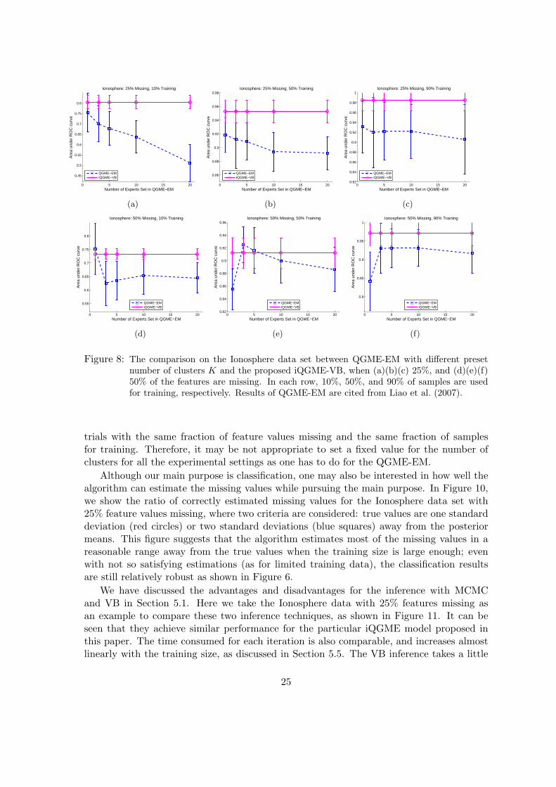
Figure 8: The comparison on the Ionosphere data set between QGME-EM with different presetnumber of clusters K and the proposed iQGME-VB, when (a)(b)(c) 25%, and (d)(e)(f)50% of the features are missing. In each row, 10%, 50%, and 90% of samples are usedfor training, respectively. Results of QGME-EM are cited from Liao et al. (2007).

trials with the same fraction of feature values missing and the same fraction of samplesfor training. Therefore, it may be not appropriate to set a fixed value for the number ofclusters for all the experimental settings as one has to do for the QGME-EM.

Although our main purpose is classification, one may also be interested in how well thealgorithm can estimate the missing values while pursuing the main purpose. In Figure 10,we show the ratio of correctly estimated missing values for the Ionosphere data set with25% feature values missing, where two criteria are considered: true values are one standarddeviation (red circles) or two standard deviations (blue squares) away from the posteriormeans. This figure suggests that the algorithm estimates most of the missing values in areasonable range away from the true values when the training size is large enough; evenwith not so satisfying estimations (as for limited training data), the classification resultsare still relatively robust as shown in Figure 6.

We have discussed the advantages and disadvantages for the inference with MCMCand VB in Section 5.1. Here we take the Ionosphere data with 25% features missing asan example to compare these two inference techniques, as shown in Figure 11. It can beseen that they achieve similar performance for the particular iQGME model proposed inthis paper. The time consumed for each iteration is also comparable, and increases almostlinearly with the training size, as discussed in Section 5.5. The VB inference takes a little

25

0 5 10 15 200

0.1

0.2

0.3

0.4

0.5

0.6

0.7

Number of Dominant Components

Pro

babi

lity

Prior and Posterior on Number of Dominant Components

PriorPosterior

(a)

0.1 0.2 0.3 0.4 0.5 0.6 0.7 0.8 0.9

1

2

3

4

5

6

7

8

9

10

11

Num

ber

of C

lust

ers



(b)

0.1 0.2 0.3 0.4 0.5 0.6 0.7 0.8 0.9

2

4

6

8

10

12

Num

ber

of C

lust

ers



(c)

Figure 9: Number of clusters for the Ionosphere data set inferred by iQGME-VB. (a) Prior andinferred posterior on the number of clusters for one trial given 10% samples for training,the number of clusters for the case when (b) 25%, and (c) 50% of features are missing.The most probable value of clusters number is used for each trial to generate (b) and (c)(e.g, the most probable value of clusters number is two for the trial shown in (a)). In (b)and (c), the distribution of number of clusters for the ten trials given each missing fractionand training fraction is presented as a box-plot, where the red line represents the median;the bottom and top of the blue box are the 25th and 75th percentile, respectively; thebottom and top black lines are the end of the whiskers, which could be the minimum andmaximum, respectively; if some data are beyond 1.5 times of the length of the blue box(interquartile range), they are outliers, indicated by a red ‘+’.

0 0.2 0.4 0.6 0.8 10.3

0.4

0.5

0.6

0.7

0.8

0.9


Rat

io o

f Mis

sing

Val

ues

Cor

rect

ly E

stim

ated


One Standard DeviationTwo Standard Deviations

Figure 10: Ratio of missing values whose true values are one standard deviation (red circles) or twostandard deviations (blue squares) away from the posterior means for the Ionospheredata set with 25% feature values missing. One trial for each training size is considered.

bit longer per iteration, probably due to the extra computation for the lower bound of thelog marginal likelihood, which serves as convergence criterion. Significant differences occuron the number of iterations we have to take. In the experiment, even though we set avery strict threshold (10−6) for the relative change of the lower bound, the VB algorithmconverges at about 50 iterations for most cases except when training data are very scarce

26

(10%). For the MCMC inference, we discard the initial samples from the first 1000 iterations(burn-in), and collect the next 500 samples to present the posterior. It is far from enoughto claim convergence; however, we consider it a fair comparison for computation as thetwo methods yield similar results under this setting. Given the fact that the VB algorithmonly takes about 1/30 the CPU time, and VB and MCMC performance are similar, inthe following examples we only present results based on VB inference. However, in all theexamples below we also performed Gibbs sampling, and the relative inference consistencyand computational costs relative to VB were found to be as summarized here (i.e., in allcases there was close agreement between the VB and MCMC inferences, and considerablecomputational acceleration manifested by VB).

0 0.2 0.4 0.6 0.8 1

0.8

0.85

0.9

0.95

1


Are

a un

der

RO

C c

urve


iQGME−VBiQGME−MCMC

(a)

0 0.2 0.4 0.6 0.8 10

0.5

1

1.5

2

2.5

3

3.5

4

4.5


Ave

rage

Tim

e fo

r E

ach

Itera

tion

(sec

onds

)



(b)

0 0.2 0.4 0.6 0.8 1

200

400

600

800

1000

1200

1400


Num

ber

of It

erat

ions



(c)

Figure 11: Comparison between VB and MCMC inferred iQGME on the Ionosphere data with 25%features missing in terms of (a) performance, (b) time consumed for each iteration, (c)number of iterations. For the VB inference, we set a threshold (10−6) for the relativechange of lower bound in two consecutive iterations as the convergence criterion; for theMCMC inference, we discard the initial samples from the first 1000 iterations (burn-in),and collect the next 500 samples to present the posterior.

6.3 Unexploded Ordnance Data

We now consider an unexploded ordnance (UXO) detection problem (Zhang et al., 2003),where two types of sensors are used to collect data, but one of them may be absent forparticular targets. Specifically, one sensor is a magnetometer (MAG) and the other anelectromagnetic induction (EMI) sensor; these sensors are deployed separately to interrogateburied targets, and for some targets both sensors are deployed and for others only one sensoris deployed. This is a real sensing problem for which missing data occurs naturally. Thedata considered were made available to the authors by the US Army (and were collectedfrom a real former bombing range in the US); the data are available to other researchersupon request. The total number of targets are 146, where 79 of them UXO and the restare non-UXO (i.e., non-explosives). A six-dimensional feature vector is extracted from theraw signals to represent each target, with the first three components corresponding to MAGfeatures and the rest as EMI features (details on feature extraction is provided in (Zhanget al., 2003)). Figure 12 shows the missing patterns for this data set.

27

Missing Pattern for the Unexploded Ordnance Data Set

Obj

ects

Features1 2 3 4 5 6

20

40

60

80

100

120

140

Figure 12: Missing pattern for the unexploded ordnance data set, where black and white indicateobserved and missing, respectively.

We compare the proposed iQGME-VB algorithm with the SVM, RVM and LR-Integrationas detailed in Section 6.2. In order to evaluate the overall performance of classifiers, werandomly partition the training and test subsets, and change the training size. Results areshown in Figure 13, where only performance means are reported for the legibility of the fig-ures. From this figure, the proposed iQGME-VB method is robust for all the experimentalsettings under both performance criteria.

0 0.2 0.4 0.6 0.8 10.65

0.7

0.75

0.8

0.85

0.9


Are

a U

nder

RO

C C

urve

AUC: BBR1 Data

RVM−Linear−UncondRVM−Linear−CondRVM−RBF−UncondRVM−RBF−CondSVM−Linear−UncondSVM−Linear−CondSVM−RBF−UncondSVM−RBF−CondLR−IntegrationiQGME−VB

(a)

0 0.2 0.4 0.6 0.8 10.6

0.65

0.7

0.75

0.8

0.85


Acc

urac

y

Accuracy: BBR1 Data

RVM−Linear−UncondRVM−Linear−CondRVM−RBF−UncondRVM−RBF−CondSVM−Linear−UncondSVM−Linear−CondSVM−RBF−UncondSVM−RBF−CondLR−IntegrationiQGME−VB

(b)

Figure 13: Mean performance over 100 random training/test partitions for each training fractionon the unexploded ordnance data set, in terms of (a) area under the ROC curve, and(b) classification accuracy.

28

6.4 Sepsis Classification Data

In Sections 6.2 and 6.3, we have demonstrated the proposed iQGME-VB on data sets withlow to moderate dimensionality. A high-dimensional data set with natural missing valuesis considered in this subsection. These data were made available to the authors from theNational Center for Genomic Research in the US, and will be made available upon request.This is another example for which missing data are a natural consequence of the sensingmodality. There are 121 patients who are infected by sepsis, with 90 of them surviving (label-1) and 31 of them who die (label 1). For each patient, we have 521 metabolic features and100 protein features. The purpose is to predict whether a patient infected by sepsis willdie given his/her features. The missing pattern of feature values is shown in Figure 14(a),where black indicates observed (this missingness is a natural consequence of the sensingdevice).

As the data are in a 621-dimensional feature space, with only 121 samples available, weuse the MFA-based variant of the iQGME (Section 2.4). To impose the low-rank belief foreach cluster, we set c0 = d0 = 1, and the largest possible dimensionality for clusters is setto be L = 50.

We compare to the same algorithms considered in Section 6.3, except the LR-Integrationalgorithm since it is not capable of handling such a high-dimensional data set. Mean AUCover ten random partitions are reported in Figure 14(b). Here we report the SVM andRVM results on the original data since they are able to classify the data in the original621-dimensional space after missing values are imputed; we also examined SVM and RVMresults on the data in a lower-dimensional latent space, after first performing factor analysison the data, and these results were very similar to the SVM/RVM results in the original621-dimensional space. From Figure 14(b), our method provides improvement by handlingmissing values analytically in the procedure of model inference and performing a dimen-sionality reduction jointly with local classifiers learning.

Missing Pattern

Pat

ient

s

Features100 200 300 400 500 600

20

40

60

80

100

120

(a)

0.1 0.2 0.3 0.4 0.5 0.6 0.7 0.8 0.9 10.86

0.87

0.88

0.89

0.9

0.91

0.92

0.93

Fraction of training data

Are

a U

nder

RO

C C

urve

AUC: Sepsis Data

RVM−Linear−UncondRVM−Linear−CondRVM−RBF−UncondRVM−RBF−CondSVM−Linear−UncondSVM−Linear−CondSVM−RBF−UncondSVM−RBF−CondiQGME−VB

(b)

Figure 14: Sepsis data set. (a) Missing pattern, where black and white indicate observed andmissing, respectively, (b) mean performance over 100 random training/test partitionsfor each training fraction.

29

6.5 Multi-Task Learning with Landmine Detection Data

We now consider a multi-task-learning example. In an application of landmine detection(available at http://www.ee.duke.edu/ lcarin/LandmineData.zip), data collected from 19landmine fields are treated as 19 subtasks. Among them, subtasks 1-10 correspond toregions that are relatively highly foliated and subtasks 11-19 correspond to regions that arebare earth or desert. In all subtasks, each target is characterized by a 9-dimensional featurevector x with corresponding binary label y (1 for landmines and -1 for clutter). The numberof landmines and clutter in each task is summarized in Figure 15. The feature vectors areextracted from images measured with airborne radar systems. A detailed description of thislandmine data set has been presented elsewhere (Xue et al., 2007).

0 5 10 15 201

10

100

1000

Index of Tasks

Num

ber

of O

bjec

ts in

Eac

h T

ask

Landmine: Number of Landmines and Clutter

LandminesClutter

Figure 15: Number of landmines and clutter in each task for the landmine-detection data set (Xueet al., 2007).

Although our main objective is to simultaneously learn classifiers for multiple taskswith incomplete data, we first demonstrate the proposed iQGME-based multi-task learning(MTL) model on the complete data, comparing it to two multi-task learning algorithmsdesigned for the situation with all the features observed. One is based on task-specificlogistic regression (LR) models, with the DP as a hierarchical prior across all the tasks(Xue et al., 2007); the other assumes an underlying structure, which is shared by allthe tasks (Ando and Zhang, 2005). For the LR-MTL algorithm, we cite results on com-plete data from (Xue et al., 2007), and implement the authors’ Matlab code with defaulthyper-parameters on the cases with incomplete data. The Matlab implementation for theStructure-MTL algorithm is included in the “Transfer Learning Toolkit for Matlab” avail-able at http://multitask.cs.berkeley.edu/. The dimension of the underlying structure isa user-set parameter, and it should be smaller than the feature dimension in the originalspace. As the dimension of the landmine detection data is 9, we set the hidden dimension as

30

5. We also tried 6, 7, and 8, and did not observe big differences in performance. Single-tasklearning (STL) iQGME and LR models are also included for comparison.

Each task is divided into training and test subsets randomly. Since the number ofelements in the two classes is highly unbalanced, as shown in Figure 15, we impose thatthere is at least one instance from each class in each subset. Following Xue et al. (2007),the size of the training subset in each task varies from 20 to 300 in increments of 20, and100 independent trials are performed for each size of data set. An average AUC (Hanleyand McNeil, 1982) over all the 19 tasks is calculated as the performance representation forone trial of a given training size. Results are reported in Figure 16.

0 50 100 150 200 250 300

0.6

0.65

0.7

0.75

0.8Landmine: Complete Data

Number of Training Samples from Each Task

Ave

rage

AU

C o

ver

19 ta

sks

LR−STLLR−MTLStructure−MTLiQGME−STLiQGME−MTL

Figure 16: Average AUC over 19 tasks of landmine detection with complete data. Error barsreflect the standard deviation across 100 random partitions of training and test subsets.Results of logistic regression based algorithms are cited from Xue et al. (2007), whereLR-MTL and LR-STL respectively correspond to SMTL-2 and STL in Figure 3 of Xueet al. (2007).

The first observation from Figure 16 is that we obtain a significant performance im-provement for single-task learning by using the iQGME-VB instead of the linear logisticregression model (Xue et al., 2007). We also notice that the multi-task algorithm based oniQGME-VB further improves the performance when the training data are scarce, and yieldscomparable overall results as the LR-MTL does. The structure-MTL does not perform wellon this data set. We suspect that a hidden structure in such a 9-dimensional space doesnot necessarily exist. Another possible reason may be that the minimization of empiricalrisk is sensitive for the cases with highly unbalanced labels, as for this data set.

It is also interesting to explore the similarity among tasks. The similarity defined by dif-ferent algorithms may be different. In (Xue et al., 2007), two tasks are defined to be similarif they share the same linear classifier. However, with the joint distribution of covariatesand the response, the iQGME-MTL requires both the data distributions and the classifica-tion boundaries to be similar if two tasks are deemed to be similar. Another difference is

31

that two tasks could be partially similar since sharing between tasks is encouraged at thecluster-level instead of at the task-level ((Xue et al., 2007) employs task-level clustering).We generate the similarity matrices between tasks as follows: In each random trial, thereare in total S higher-level items shared among tasks. For each task, we can find the task-specific probability mass function (pmf) over all the higher-level items. Using these pmfs asthe characteristics for tasks in the current trial, we calculate the pair-wise Kullback-Leibler(KL) distances and convert them to similarity measures through a minus exponential func-tion. Results of multiple trials are summed over and normalized as shown in Figure 17. Itcan be seen that the similarity structure among tasks becomes clearer when we have moretraining data available. As discovered by Xue et al. (2007), we also find two big clusterscorrespond to two different vegetation conditions of the landmine fields (task 1-10 and task11-19). Further sub-structures among tasks are also explored by the iQGME-MTL model,which may suggest other unknown difference among the landmine fields.

2 4 6 8 10 12 14 16 18

2

4

6

8

10

12

14

16

18

Index of Task

Inde

x of

Tas

k

(a)

2 4 6 8 10 12 14 16 18

2

4

6

8

10

12

14

16

18

Index of Task

Inde

x of

Tas

k

(b)

2 4 6 8 10 12 14 16 18

2

4

6

8

10

12

14

16

18

Index of Task

Inde

x of

Tas

k

(c)

Figure 17: Similarity between tasks in the landmine detection problem with complete data given(a) 20, (b) 100, and (c) 300 training samples from each task. The size of green blocksrepresent the value of the corresponding matrix element.

After yielding competitive results on the landmine-detection data set with completedata, the iQGME-based algorithms are evaluated on incomplete data, which are simulatedby randomly removing a portion of feature values for each task as in Section 6.2. We considerthree different portions of missing values: 25%, 50% and 75%. As in the experiments aboveon benchmark data sets, we perform ten independent random trials for each setting ofmissing fraction and training size.

To the best of our knowledge, there exists no previous work in the literature on multi-tasklearning with missing data. As presented in Figure 18, we use the LR-MTL (Xue et al., 2007)and the Structure-MTL (Ando and Zhang, 2005) with missing values imputed as baselinealgorithms. Results of the two-step LR with integration (Williams et al., 2007) and theLR-STL with single imputations are also included for comparison. Imputations using bothunconditional-means and conditional-means are considered. From Figure 18, iQGME-STLconsistently performs best among single-task learning methods and even better than LR-MTL-Uncond when the size of the training set is relatively large. The imputations using

32

0 50 100 150 200 250 300

0.56

0.58

0.6

0.62

0.64

0.66

0.68

0.7

0.72

0.74

0.76

Landmine: 25% Features Missing


Ave

rage

AU

C o

ver

19 ta

sks

LR−STL−UncondLR−MTL−UncondLR−STL−CondLR−MTL−CondLR−IntegrationStructure−MTL−UncondStructure−MTL−CondiQGME−STLiQGME−MTL

(a)

0 50 100 150 200 250 3000.5

0.55

0.6

0.65

0.7



Ave

rage

AU

C o

ver

19 ta

sks


(b)

0 50 100 150 200 250 300

0.48

0.5

0.52

0.54

0.56

0.58

0.6

0.62

0.64

0.66

0.68



Ave

rage

AU

C o

ver

19 ta

sks


(c)

Figure 18: Average AUC over 19 tasks of landmine detection for the cases when (a) 25%, (b) 50%,and (c) 75% of the features are missing. Mean values of performance across 10 randompartitions of training and test subsets are reported. Error bars are omitted for legibility.

conditional-means yields consistently better results for the LR-based models on this dataset. The iQGME-MTL outperforms the baselines and all the single-task learning methodsoverall. Furthermore, the improvement of iQGME-MTL is more pronounced when there aremore features missing. These observations underscore the advantage of handling missingdata in a principled manner and at the same time learning multiple tasks simultaneously.

The task-similarity matrices for the incomplete-data cases are shown in Figure 19. Itcan be seen that when a small fraction (e.g., 25%) of the feature values are missing andtraining data are rich (e.g., 300 samples from each task), the similarity pattern amongtasks is similar to what we have seen for the complete-data case. As the fraction of missingvalues becomes larger, tasks appear more different from each other in terms of the usageof the higher-level items. Considering that the missing pattern for each task is unique, itis probable that tasks look quite different from each other after a large fraction of featurevalues are missing. However, the fact that tasks tend to use different subsets of higher-level

33

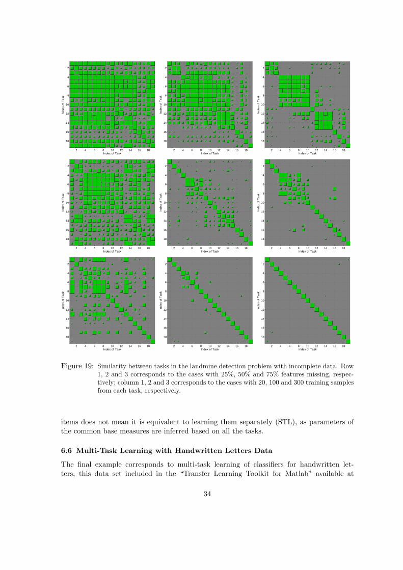
2 4 6 8 10 12 14 16 18

2

4

6

8

10

12

14

16

18

Index of Task

Inde

x of

Tas

k

2 4 6 8 10 12 14 16 18

2

4

6

8

10

12

14

16

18

Index of Task

Inde

x of

Tas

k

2 4 6 8 10 12 14 16 18

2

4

6

8

10

12

14

16

18

Index of Task

Inde

x of

Tas

k

2 4 6 8 10 12 14 16 18

2

4

6

8

10

12

14

16

18

Index of Task

Inde

x of

Tas

k

2 4 6 8 10 12 14 16 18

2

4

6

8

10

12

14

16

18

Index of Task

Inde

x of

Tas

k

2 4 6 8 10 12 14 16 18

2

4

6

8

10

12

14

16

18

Index of Task

Inde

x of

Tas

k

2 4 6 8 10 12 14 16 18

2

4

6

8

10

12

14

16

18

Index of Task

Inde

x of

Tas

k

2 4 6 8 10 12 14 16 18

2

4

6

8

10

12

14

16

18

Index of Task

Inde

x of

Tas

k

2 4 6 8 10 12 14 16 18

2

4

6

8

10

12

14

16

18

Index of Task

Inde

x of

Tas

k

Figure 19: Similarity between tasks in the landmine detection problem with incomplete data. Row1, 2 and 3 corresponds to the cases with 25%, 50% and 75% features missing, respec-tively; column 1, 2 and 3 corresponds to the cases with 20, 100 and 300 training samplesfrom each task, respectively.

items does not mean it is equivalent to learning them separately (STL), as parameters ofthe common base measures are inferred based on all the tasks.

6.6 Multi-Task Learning with Handwritten Letters Data

The final example corresponds to multi-task learning of classifiers for handwritten let-ters, this data set included in the “Transfer Learning Toolkit for Matlab” available at

34

http://multitask.cs.berkeley.edu/. The objective of each task is to distinguish two letterswhich are easily confused. The number of samples for all the letters considered in the totaleight tasks is summarized in Table 2. Each sample is a 16× 8 image as shown in Figure 20.We use the 128 pixel values of each sample directly as its feature vector.

Table 2: Handwritten letters classification data set.Task 1 Task 2 Task 3 Task 4 Task 5 Task 6 Task 7 Task 8

‘c’: 2107 ‘g’: 2460 ‘m’: 1596 ‘a’: 4016 ‘i’: 4895 ‘a’: 4016 ‘f’: 918 ‘h’: 858‘e’: 4928 ‘y’: 1218 ‘n’: 5004 ‘g’: 2460 ‘j’: 188 ‘o’: 3880 ‘t’: 2131 ‘n’: 5004

Figure 20: Sample images of the handwritten letters. The two images in each column representsthe two classes in the corresponding task described in Table 2.

We compare the proposed iQGME-MTL algorithm to the LR-MTL (Xue et al., 2007)and the Structure-MTL (Ando and Zhang, 2005) mentioned in Section 6.5. For the non-parametric Bayesian methods (iQGME-MTL and LR-MTL), we use the same parametersetting as before. The dimension of the underlying structure for the Structure-MTL is setto be 50 in the results shown in Figure 21. We also tried 10, 20, 40, 60, 80 and 100, anddid not observe big difference. From Figure 21, the iQGME-MTL performs significantlybetter than the baselines on this data set for all the missing fractions and training fractionsunder consideration. As we expected, the Structure-MTL yields comparable results as theLR-MTL on this data set.

7. Conclusion and Future Work

In this paper we have introduced three new concepts, summarized as follows. First, we haveemployed non-parametric Bayesian techniques to develop a mixture-of-experts algorithmfor classifier design, which employs a set of localized (in feature space) linear classifiers asexperts. The Dirichlet process is employed to allow the model to infer automatically theproper number of experts and their characteristics; in fact, since a Bayesian formulation isemployed, a full posterior distribution is manifested on the properties of the local experts,including their number. Secondly, the classifier is endowed with the ability to naturallyaddress missing data, without the need for an imputation step. Finally, the whole frameworkhas been placed within the context of a multi-task learning, allowing one to jointly inferclassifiers for multiple data sets with missing data. The multi-task-learning component hasalso been implemented with the general tools associated with the Dirichlet process, withspecific implementations manifested via the hierarchical Dirichlet process. Because of thehierarchical form of the model, in terms of a sequence of distributions in the conjugate-exponential family, all inference has been manifested efficiently via variational Bayesian

35

100 200 300 400 500

0.86

0.87

0.88

0.89

0.9

0.91

0.92

0.93

0.94

0.95

0.96Handwritten Letters: Complete

Number of training samples from each task

Ave

rage

AU

C o

ver

eigh

t tas

ks

LR−MTLStructure−MTLiQGME−MTL

(a)

100 200 300 400 500

0.84

0.86

0.88

0.9

0.92

0.94

0.96Handwritten Letters: 25% Features Missing


Ave

rage

AU

C o

ver

eigh

t tas

ks

LR−MTL−UncondLR−MTL−CondStructure−MTL−UncondStructure−MTL−CondiQGME−MTL

(b)

100 200 300 400 5000.78

0.8

0.82

0.84

0.86

0.88

0.9

0.92

Handwritten Letters: 50% Features Missing


Ave

rage

AU

C o

ver

eigh

t tas

ks


(c)

100 200 300 400 500

0.7

0.72

0.74

0.76

0.78

0.8

0.82

0.84

0.86

0.88

Handwritten: 75% Features Missing


Ave

rage

AU

C o

ver

eigh

t tas

ks


(d)

Figure 21: Average AUC over eight tasks of handwriting letters classification for the cases when(a) none, (b) 25%, (c) 50%, and (d) 75% of the features are missing. Mean values ofperformance with one standard deviation across 10 random partitions of training andtest subsets are reported.

(VB) analysis. The VB results have been compared to those computed via Gibbs sampling;the VB results have been found to be consistent with those inferred via Gibbs sampling,while requiring a small fraction of the computational costs. Results have been presentedfor single-task and multi-task learning on various data sets with the same hyper-parameterssetting (no model-parameter tuning), and encouraging algorithm performance has beendemonstrated.

Concerning future research, we note that the use of multi-task learning provides animportant class of contextual information, and therefore is particularly useful when one haslimited labeled data and when the data are incomplete (missing features). Another formof context that has received significant recent attention is semi-supervised learning (Zhu,2005). There has been recent work on integrating multi-task learning with semi-supervised

36

learning (Liu et al., 2007). An important new research direction includes extending semi-supervised multi-task learning to realistic problems for which the data are incomplete.

Appendix

The update equations of single-task learning with incomplete data are summarized as fol-lows:

1. q(ti|µti)

µti =

N∑

h=1

ρih〈wh〉T xbi,h where xb

i,h = [xoii ; mmi|oi

h ; 1].

The expectation of ti and t2i may be derived according to properties of truncatednormal distributions:

〈ti〉 = µti +

φ(−µti)

1(yi = 1)− Φ(−µti)

,

〈t2i 〉 = 1 + (µti)

2 +µt

iφ(−µti)

1(yi = 1)− Φ(−µti)

,

where φ(·) and Φ(·) denote the probability density function and the cumulative densityfunction of the standard normal distribution, respectively.

2. q(xmii , zi|mmi|oi

ih ,Σmi|oi

ih , ρih)A related derivation for a GMM model with incomplete data could be found in(Williams et al., 2007), where no classifier terms appear.

First, we explicitly write the intercept wbh , that is, wh = [(wx

h)T , wbh]T :

q(xmii , zi = h)

∝ exp〈ln[p(ti|zi = h,xi, W )p(zi = h|V )p(xi|zi = h,µ,Λ)]〉q(ti)q(wh)q(V )q(µh,Λh)∝ AihNP (xi|µih, Σih),

where

Σih = [〈wxh(wx

h)T 〉+ νhBh]−1

µih = Σih[〈ti〉〈wxh〉+ νhBhmh − 〈wx

hwbh〉]

Aih = exp〈lnVh〉+∑

l<h

〈ln(1− Vl)〉+ 〈ti〉〈wbh〉

+12[〈ln |Λh|〉+ µT

ihΣ−1ih µih + ln |Σih| − P

uh−mT

h νhBhmh − 〈(wbh)

2〉].

Since[

xoii

xmii

]∼ NP

([µoi

ih

µmiih

],

[Σoioi

ih Σoimiih

Σmioiih Σmimi

ih

]),

37

the conditional distribution of missing features xmii given observable features xoi

i isalso a normal distribution, that is, xmi

i |xoii ∼ N|mi|(m

mi|oi

h ,Σmi|oi

h ) with

mmi|oi

h = µmiih + Σmioi

ih (Σoioiih )−1(xoi

i − µoiih),

Σmi|oi

h = Σmimiih − Σmioi

ih (Σoioiih )−1Σoimi

ih .

Therefore, q(xmii , zi = h) could be factorized as the product of a factor independent

of xmii and the variational posterior of xmi

i , that is,

q(xmii , zi = h) ∝ AihN|oi|(x

oii |µoi

ih, Σoioiih )N|mi|(x

mii |mmi|oi

h ,Σmi|oi

h )

ρih ∝ AihN|oi|(xoii |µoi

ih, Σoioiih )

For complete data, no factorization for the distribution for xmii is necessary:

ρih ∝ exp〈ti〉〈wh〉T xi − 12xT

i 〈whwTh 〉xi + 〈ln Vh〉

+∑

l<h

〈ln(1− Vl)〉+12〈ln |Λh|〉 − 1

2〈(xi − µh)TΛh(xi − µh)〉

3. q(Vh|vh1, vh2)

Similar updating could be found in (Blei and Jordan, 2006), except that we put aprior belief on α here instead of setting a fixed number.

vh1 = 1 +n∑

i=1

ρih, vh2 = 〈α〉+n∑

i=1

∑

l>h

ρil;

〈ln Vh〉 = ψ(vh1)− ψ(vh1 + vh2), 〈ln(1− Vl)〉 = ψ(vl2)− ψ(vl1 + vl2).

4. q(µh,Λh|mh, uh, Bh, νh)

Similar updating could be found in (Williams et al., 2007).

νh = ν0 + Nh, uh = u0 + Nh, mh =u0m0 + Nhxh

uh,

B−1h = B−1

0 +n∑

i=1

ρihΩi,h + NhSh +u0Nh

uh(xh −m0)(xh −m0)T ,

where

Nh =n∑

i=1

ρih, xh =n∑

i=1

ρihxi/Nh, Sh =n∑

i=1

ρih(xi,h − xh)(xi,h − xh)T /Nh.

xi,h =

[xoi

i

mmi|oi

h

], Ωi,h =

[0 00 Σmi|oi

h

].

〈ln |Λh|〉 =P∑

p=1

ψ((νh − p + 1)/2) + P ln 2 + ln |Bh|,

〈(xi − µh)TΛh(xi − µh)〉 = (xi,h −mh)T νhBh(xi,h −mh) + P/uh + tr(νhBhΩi,h).

38

5. q(wh|µwh ,Σw

h ), 〈wh〉 = µwh , 〈whwT

h 〉 = Σwh + µw

h (µwh )T .

Σwh =

(n∑

i=1

ρih(Ωi,h + xbi,hxb

T

i,h) + diag(〈λ〉))−1

,

µwh = Σw

h

(n∑

i=1

ρihxbi,h〈ti〉+ diag(〈λ〉)φ

).

6. q(ζp, λp|φp, γ, ap, bp), 〈λp〉 = ap/bp.

Similar updating could be found in (Xue et al., 2007).

φp =N∑

h=1

〈whp〉/γ, γ = γ0 + N

ap = a0 +N

2, bp = b0 +

12

N∑

h=1

〈w2hp〉 −

12γφ2

p.

7. q(α|τ1, τ2), 〈α〉 = τ1/τ2.

Similar updating could be found in any VB-inferred DP model with a Gamma prioron α (Xue et al., 2007).

τ1 = N − 1 + τ10, τ2 = τ20 −N−1∑

h=1

〈ln(1− Vh)〉.

The update equations of multi-task learning with incomplete data are summarized asfollows:

1. q(tji|µtji)

µtji =

S∑

s=1

Eσjis〈ws〉T xbji where Eσjis =

N∑

h=1

ρjihσjhs, xbji = [xoji

ji ; mmji|oji

ji ; 1].

2. q(xmji

ji |mmji|oji

ji ,Σmji|oji

ji )

mmji|oji

ji = µmji

ji + Σmjioji

ji (Σojioji

ji )−1(xoji

ji − µoji

ji ),

Σmji|oji

ji = Σmjimji

ji − Σmjioji

ji (Σojioji

ji )−1Σojimji

ji ,

where

Σji =

(S∑

s=1

Eσjis(〈wxs (wx

s )T 〉+ νsBs)

)−1

,

µji = Σji

S∑

s=1

Eσjis(〈tji〉〈wxs 〉+ νsBsms − 〈wx

s wbs〉).

39

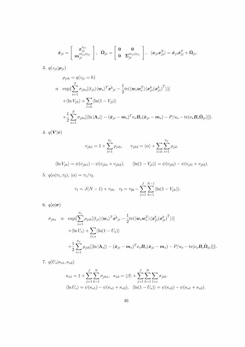
xji =

[x

oji

ji

mmji|oji

ji

], Ωji =

[0 00 Σmji|oji

ji

], 〈xjix

Tji〉 = xjix

Tji + Ωji.

3. q(zji|ρji)

ρjih = q(zji = h)

∝ expS∑

s=1

σjhs[〈tji〉〈ws〉T xbji − 1

2tr(〈wsw

Ts 〉〈xb

ji(xbji)

T 〉)]

+〈lnVjh〉+∑

l<h

〈ln(1− Vjl)〉

+12

S∑

s=1

σjhs[〈ln |Λs|〉 − (xji −ms)T νsBs(xji −ms)− P/us − tr(νsBsΩji)].

4. q(V |v)

vjh1 = 1 +nj∑

i=1

ρjih, vjh2 = 〈α〉+∑

l>h

nj∑

i=1

ρjil.

〈lnVjh〉 = ψ(vjh1)− ψ(vjh1 + vjh2), 〈ln(1− Vjl)〉 = ψ(vjl2)− ψ(vjl1 + vjl2).

5. q(α|τ1, τ2), 〈α〉 = τ1/τ2.

τ1 = J(N − 1) + τ10, τ2 = τ20 −J∑

j=1

N−1∑

h=1

〈ln(1− Vjh)〉.

6. q(c|σ)

σjhs ∝ expnj∑

i=1

ρjih[〈tji〉〈ws〉T xbji − 1

2tr(〈wsw

Ts 〉〈xb

ji(xbji)

T 〉)]

+〈ln Us〉+∑

l<s

〈ln(1− Us)〉

+12

nj∑

i=1

ρjih[〈ln |Λs|〉 − (xji −ms)T νsBs(xji −ms)− P/us − tr(νsBsΩji)].

7. q(Us|κs1, κs2)

κs1 = 1 +J∑

j=1

N∑

h=1

σjhs, κs2 = 〈β〉+J∑

j=1

N∑

h=1

∑

l>s

σjhl.

〈lnUs〉 = ψ(κs1)− ψ(κs1 + κs2), 〈ln(1− Us)〉 = ψ(κs2)− ψ(κs1 + κs2).

40

8. q(β|τ3, τ4), 〈β〉 = τ3/τ4.

τ3 = S − 1 + τ30, τ4 = τ40 −S−1∑

s=1

〈ln(1− Us)〉.

9. q(µs,Λs|ms, us, Bs, νs)

νs = ν0 + Ns, us = u0 + Ns, ms =u0m0 + Nsxs

us,

B−1s = B−1

0 +J∑

j=1

nj∑

i=1

EσjisΩji + NsSs +u0Ns

us(xs −m0)(xs −m0)T ,

where Eσjis =∑N

h=1 ρjihσjhs, and

Ns =J∑

j=1

nj∑

i=1

Eσjis, xs =J∑

j=1

nj∑

i=1

Eσjisxji/Ns,

Ss =J∑

j=1

nj∑

i=1

Eσjis(xji − xs)(xji − xs)T /Ns.

〈ln |Λs|〉 =P∑

p=1

ψ((νs − p + 1)/2) + P ln 2 + ln |Bs|,

〈(xji − µs)TΛs(xji − µs)〉 = (xji −ms)T νsBs(xji −ms) + P/us + tr(νsBsΩji).

10. q(ws|µws ,Σw

s )

Σws =

J∑

j=1

nj∑

i=1

Eσjis(xbjixb

T

ji + Ωji) + diag(〈λ〉)−1

,

µws = Σw

s

J∑

j=1

nj∑

i=1

Eσjisxbji〈tji〉+ diag(〈λ〉)φ

.

〈ws〉 = µws , 〈wsw

Ts 〉 = Σw

s + µws (µw

s )T .

11. q(λp|ap, bp), 〈λp〉 = ap/bp.

φp =S∑

s=1

〈wsp〉/γ, γ = γ0 + S,

ap = a0 +S

2, bp = b0 +

12

S∑

s=1

〈W 2sp〉 −

12γφ2

p.

41

References

J. H. Albert and S. Chib. Bayesian analysis of binary and polychotomous response data.Journal of the American Statistical Association, 88:669–679, 1993.

R. K. Ando and T. Zhang. A framework for learning predictive structures from multipletasks and unlabeled data. Journal of Machine Learning Research, 6:1817–1853, 2005.

H. Attias. A variational Bayesian framework for graphical models. In Advances in NeuralInformation Processing Systems (NIPS), 2000.

M. J. Beal. Variational Algorithms for Approximate Bayesian Inference. PhD dissertation,University College London, Gatsby Computational Neuroscience Unit, 2003.

D. M. Blei and M. I. Jordan. Variational inference for Dirichlet process mixtures. BayesianAnalysis, 1(1):121–144, 2006.

R. Caruana. Multitask learning. Machine Learning, 28:41–75, 1997.

G. Chechik, G. Heitz, G. Elidan, P. Abbeel, and D. Koller. Max-margin classification ofdata with absent features. Journal of Machine Learning Research, 9:1–21, 2008.

L. M. Collins, J. L. Schafer, and C. M. Kam. A comparison of inclusive and restrictivestrategies in modern missing data procedures. Psychological Methods, 6(4):330–351, 2001.

A. Dempster, N. Laird, and D. Rubin. Maximum likelihood from incomplete data via theEM algorithm. Journal of Royal Statistical Society B, 39:1–38, 1977.

U. Dick, P. Haider, and T. Scheffer. Learning from incomplete data with infinite imputa-tions. In International Conference on Machine Learning (ICML), 2008.

D. B. Dunson, N. Pillai, and J.-H. Park. Bayesian density regression. Journal of the RoyalStatistical Society: Series B, 69, 2007.

M. D. Escobar and M. West. Bayesian density estimation and inference using mixtures.Journal of the American Statistical Association, 90:577–588, 1995.

T. Ferguson. A Bayesian analysis of some nonparametric problems. The Annals of Statistics,1:209–230, 1973.

A. E. Gelfand, S. E. Hills, A. Racine-Poon, and A. F. M. Smith. Illustration of Bayesianinference in normal data models using Gibbs sampling. Journal of American StatisticalAssociation, 85:972–985, 1990.

Z. Ghahramani and M. J. Beal. Variational inference for Bayesian mixtures of factor anal-ysers. In Advances in Neural Information Processing Systems (NIPS) 12, pages 449–455.MIT Press, 2000.

Z. Ghahramani and G. E. Hinton. The EM algorithm for mixtures of factor analyzers.Technical Report CRG-TR-96-1, Department of Computer Science, University of Toronto,1996.

42

Z. Ghahramani and M. I. Jordan. Learning from incomplete data. Technical report, Mas-sachusetts Institute of Technology, 1994.

T. Graepel. Kernel matrix completion by semidefinite programming. In Proceedings of theInternational Conference on Artificial Neural Networks, pages 694–699, 2002.

J. Hanley and B. McNeil. The meaning and use of the area under a receiver operatingcharacteristic (roc) curve. Radiology, 143:29–36, 1982.

L. Hannah, D. Blei, and W. Powell. Dirichlet process mixtures of generalized linear models.In Artificial Intelligence and Statistics (AISTATS), pages 313–320, 2010.

J. Ibrahim. Incomplete data in generalized linear models. Journal of the American StatisticalAssociation, 85:765–769, 1990.

H. Ishwaran and L. F. James. Gibbs sampling methods for stick-breaking priors. Journalof the American Statistical Association, 96:161–173, 2001.

R. A. Jacobs, M. I. Jordon, S. J. Nowlan, and G. E. Hinton. Adaptive mixtures of localexperts. Neural Computation, 3:79–87, 1991.

M. I. Jordan and R. A. Jacobs. Hierarchical mixtures of experts and the EM algorithm.Neural Computation, 6:181–214, 1994.

K. Kurihara, M. Welling, and Y. W. Teh. Collapsed variational Dirichlet process mixturemodels. In Proceedings of the International Joint Conference on Artificial Intelligence(IJCAI), pages 2796–2801, 2007.

Percy Liang and Michael I. Jordan. An asymptotic analysis of generative, discriminative,and pseudolikelihood estimators. In Proceedings of the International Conference on Ma-chine Learning (ICML), pages 584–591, 2008.

X. Liao, H. Li, and L. Carin. Quadratically gated mixture of experts for incompletedata classification. In Proceedings of the International Conference on Machine Learn-ing (ICML), pages 553–560, 2007.

Q. Liu, X. Liao, and L. Carin. Semi-supervised multitask learning. In Neural InformationProcessing Systems, 2007.

S. N. MacEachern and P. Muller. Estimating mixture of dirichlet process models. Journalof Computational and Graphical Statistics, 7, 1998.

E. Meeds and S. Osindero. An alternative infinite mixture of Gaussian process experts. InNIPS 18, pages 883–890. MIT Press, 2006.

P. Muller, A. Erkanli, and M. West. Bayesian curve fitting using multivariate normalmixtures. Biometrika, 83:67–79, 1996.

R. M. Neal. Probabilistic inference using Markov chain Monte Carlo methods. Technicalreport, Department of Computer Science, University of Toronto, 1993.

43

D. J. Newman, S. Hettich, C. L. Blake, and C. J. Merz. UCI repository of machine learningdatabases. http://www.ics.uci.edu/∼mlearn/MLRepository.html, 1998.

A. Y. Ng and M. I. Jordan. On discriminative vs. generative classifiers: A comparisonof logistic regression and naive Bayes. In Advances in Neural Information ProcessingSystems (NIPS), 2002.

C. E. Rasmussen and Z. Ghahramani. Infinite mixtures of Gaussian process experts. InNIPS 14. MIT Press, 2002.

A. Rodrıguez, D. B. Dunson, and A. E. Gelfang. Bayesian nonparametric functional dataanalysis through density estimation. Biometrika, 96, 2009.

D. B. Rubin. Inference and missing data. Biometrika, 63:581–592, 1976.

D. B. Rubin. Multiple Imputation for Nonresponse in Surveys. John Wiley & Sons, Inc.,1987.

J. L. Schafer and J. W. Graham. Missing data: Our view of the state of the art. PsychologicalMethods, 7:147–177, 2002.

J. Sethuraman. A constructive definition of Dirichlet priors. Statistica Sinica, 1:639–650,1994.

B. Shahbaba and R. Neal. Nonlinear models using Dirichlet process mixtures. Journal ofMachine Learning Research, 10:1829–1850, 2009.

P. K. Shivaswamy, C. Bhattacharyya, and A. J. Smola. Second order cone programming ap-proaches for handling missing and uncertain data. Journal of Machine Learning Research,7:1283–1314, 2006.

A. Smola, S. Vishwanathan, and T. Hofmann. Kernel methods for missing variables. InProceedings of the Tenth International Workshop on Artificial Intelligence and Statistics,2005.

Y. W. Teh, M. J. Beal M. I. Jordan, and D. M. Blei. Hierarchical Dirichlet processes.Journal of the American Statistical Association, 101:1566–1581, 2006.

M. E. Tipping. The relevance vector machine. In T. K. Leen S. A. Solla and K. R. Muller,editors, Advances in Neural Information Processing Systems (NIPS), volume 12, pages652–658. MIT Press, 2000.

V. N. Vapnik. The Nature of Statistical Learning Theory. Springer, 1995.

X. Wang, A. Li, Z. Jiang, and H. Feng. Missing value estimation for dna microarray geneexpression data by support vector regression imputation and orthogonal coding scheme.BMC Bioinformatics, 7:32, 2006.

S. R. Waterhouse and A. J. Robinson. Classification using hierarchical mixtures of experts.In Proceedings of the IEEE Workshop on Neural Networks for Signal Processing IV, pages177–186, 1994.

44

M. West, P. Muller, and M. D. Escobar. Hierarchical priors and mixture models, withapplication in regression and density estimation. In P. R. Freeman and A. F. Smith,editors, Aspects of Uncertainty, pages 363–386. John Wiley, 1994.

D. Williams and L. Carin. Analytical kernel matrix completion with incomplete multi-view data. In Proceedings of the International Conference on Machine Learning (ICML)Workshop on Learning with Multiple Views, pages 80–86, 2005.

D. Williams, X. Liao, Y. Xue, L. Carin, and B. Krishnapuram. On classification withincomplete data. IEEE Transactions on Pattern Analysis and Machine Intelligence, 29(3):427–436, 2007.

L. Xu, M. I. Jordan, and G. E. Hinton. An alternative model for mixtures of experts. InAdvances in Neural Information Processing Systems (NIPS) 7, pages 633–640, 1995.

Y. Xue, X. Liao, L. Carin, and B. Krishnapuram. Multi-task learning for classification withDirichlet process priors. Journal of Machine Learning Research, 8:35–63, 2007.

K. Yu, A. Schwaighofer, V. Tresp, W.-Y. Ma, and H. Zhang. Collaborative ensemblelearning: Combining collaborative and content-based information filtering via hierarchicalBayes. In Proceedings of the Conference on Uncertainty in Artificial Intelligence, pages616–623, 2003.

J. Zhang, Z. Ghahramani, and Y. Yang. Learning multiple related tasks using latent in-dependent component analysis. In Advances in Neural Information Processing Systems,2006.

Y. Zhang, L. M. Collins, H. Yu, C. Baum, and L. Carin. Sensing of unexploded ordnancewith magnetometer and induction data: theory and signal processing. IEEE Transactionson Geoscience and Remote Sensing, 41(5):1005–1015, 2003.

X. Zhu. Semi-supervised learning literature survey. Technical Report 1530, ComputerSciences, University of Wisconsin-Madison, 2005.

45

Classiﬂcation with Incomplete Data Using Dirichlet Process...

Documents

Transcript of Classiﬂcation with Incomplete Data Using Dirichlet Process...