Classifying Music Based on Frequency Content and Audio Data

Craig DennisECE 539

Final Report

Introduction

With the growing market of portable digital audio players, the number of digital

music files inside personal computers has increased. It can be difficult to choose and

classify which songs to listen to when you want to listen to specific genres of music, such

as classical music, pop music and classic rock. Not only must the consumer classify their

music, but online distributors must classify thousands of songs in their databases for their

consumers to browse through.

How can music be easily classified without human interaction? It would be

extremely tedious to go through all of the songs in a large database one by one to classify

them. A neural network could be trained to determine the difference between three

different genres of music, classical music, pop and classic rock.

For this project, I have taken 30 sample songs from 3 genres of music, classical

music, pop music and classic rock music and analyzed the middle five seconds to classify

the music. Frequency content of the audio files can be extracted using the Fast Fourier

Transform in Matlab. The songs were recorded at a sampling rate of 44.1Khz, so the

largest recoverable frequency is 22.05Khz. The five second samples were broken down

further to take the short time Fourier transform of 50 millisecond samples. These samples

were broken down into the low frequency content (0-200Hz), lower middle frequency

content (201-400Hz), higher middle frequency content (400-800Hz) and into further

higher bands (800-1600Hz), (1600-3200Hz) and (3200-22050Hz.) These frequency

bands can help describe the acoustic characteristics of the sample. The 50ms samples

were averaged within 250ms samples. This gave 120 features to classify the song. The

frequency bands were chosen because they are ranges in which different musical

instruments are found. Most bass instruments are within the 50-200Hz range. Many brass

instruments like the trumpet and French horn are within the 200-800Hz range.

Woodwinds are roughly found in 800-1600Hz. The higher frequencies were chosen

because many classic rock songs and pop songs have distorted guitars which have high

frequency content in their noise.

The 120 feature vectors were classified using the K-Nearest Neighbor neural

network as well as the Multi-Layer Perceptron neural network.

Problem Statement

Given a specific song, I would like a neural network to classify that song in a

specific genre, either classic rock, pop, or classical music.

Motivation

I enjoy listening to music. I have thousands of MP3s on my computer and over a

hundred CDs at home. Sometimes I feel like listening to a specific type of music, not

exactly a specific song or group, but just a certain type of music. Sometimes I feel like

relaxing to some smooth classical music and other times I feel like listening to some

guitar solos. Most of the music is only classified by the artist, album and song name. This

is excellent information, but it doesn’t help me choose a song when I’m in a certain

mood. If all of my music was classified by a specific genre, it would be much easier to

help me find a song to listen to.

Different genres of music can sound very different from one another. Most

classical music I listen to has nice string arrangements and very little bass. The classic

rock songs I listen to normally contain a big guitar solo, with a lot of distortion and noise.

The pop music I listen to has groovy bass lines and great vocals. All of the instruments in

the different genres are in different frequency ranges. I thought that if I was able to pick

out the certain frequencies for songs, I could feed them into a neural network to help

classify the songs.

Work Performed

Data Collection

To collect data for this project, I had to collect 30 songs from 3 different genres:

classic rock, pop and classical music. All of the songs were extracted from a CD to a

wave file on my computer. The wave files are uncompressed music from CDs that were

recorded at 44.1Khz. Each song was anywhere between 30 to 90 megabytes in size. I had

a total of about 4 Gigabytes of music data to analyze. I decided not to use MP3 files for

my data collection because MP3s can be encoded at different bit rates with different

encoders. The same song could be encoded with different encoders at the same bit rate or

the same encoder with different bit rates and the MP3 files would contain different data.

By choosing wave files, I eliminated that problem.

To try to classify the music, I needed to decide which features I wanted to extract

from the song. The first feature I decided to extract was the song length. I used this

feature since it is easy to calculate and could be very useful in classifying songs. I also

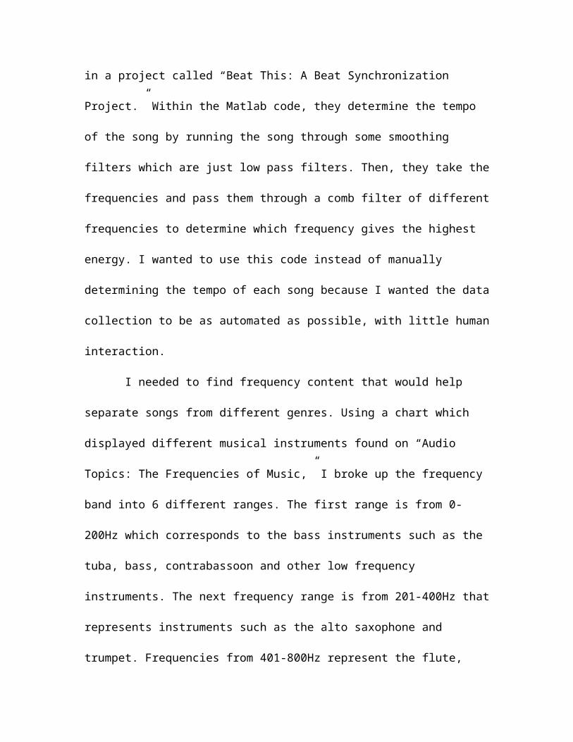
wanted to find the tempo of the song. I found Matlab code online from Rice University in

a project called “Beat This: A Beat Synchronization Project.” Within the Matlab code,

they determine the tempo of the song by running the song through some smoothing filters

which are just low pass filters. Then, they take the frequencies and pass them through a

comb filter of different frequencies to determine which frequency gives the highest

energy. I wanted to use this code instead of manually determining the tempo of each song

because I wanted the data collection to be as automated as possible, with little human

interaction.

I needed to find frequency content that would help separate songs from different

genres. Using a chart which displayed different musical instruments found on “Audio

Topics: The Frequencies of Music,” I broke up the frequency band into 6 different

ranges. The first range is from 0-200Hz which corresponds to the bass instruments such

as the tuba, bass, contrabassoon and other low frequency instruments. The next frequency

range is from 201-400Hz that represents instruments such as the alto saxophone and

trumpet. Frequencies from 401-800Hz represent the flute, high notes on the violin and

guitar. The 801-1600Hz range has instruments such as the piccolo and high notes on the

harp. The next frequency range is from 1601-3200Hz that represents high frequency

content and some harmonic frequencies. The frequency range from 3201-22050Hz

contain the very high frequencies that humans can barely hear and is the limit of

frequencies that can be heard on a CD.

To get these frequencies, I used the FFT function in Matlab to convert the wave

files from the time domain to the frequency domain. Originally I wanted to convert the

whole song to the frequency domain for analysis; however, Matlab ran out of memory

and crashed. It was trying to use over 2 Gigabytes of memory. I decided to only sample a

piece of the song to represent all of the song’s data. I decided to use the middle 5 seconds

of each song. This time frame was chosen because the middle of a song is normally

where the chorus is found. I did not want to take the first few seconds of a song because

the introduction is not always where the main theme of the song is found. I also did not

want to sample the last few seconds of a song because the song could either fade out or

crescendo to a peak, neither of which really represents the song.

I wanted to try to determine how the song changed during time, so I broke the 5

second sample down to little 50ms chunks. This is similar to how Yibin Zhang and Jie

Zhou sampled their songs for classification, however they used 45ms samples. I took the

FFT of each 50ms sample in the 6 different frequency bands. Then, I averaged the

magnitudes of the 6 frequency bands in 250ms samples to get a total of 120 different

features. I had 20 different samples through time ranging through 6 different frequency

bands for the 5 second sample.

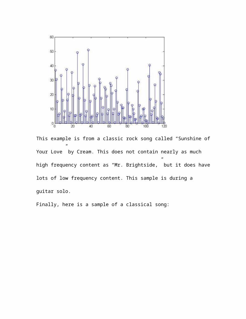
Here is an example of what the data looks like:

This is an example from a pop song called “Mr. Brightside” by The Killers. Notice all of

the high frequency content throughout the entire sample. Also notice that all of the

frequencies are rather loud throughout the entire frequency spectrum. This sample is

during the verse of the song.

Here is another example of data from another song:

This example is from a classic rock song called “Sunshine of Your Love” by Cream. This

does not contain nearly as much high frequency content as “Mr. Brightside,” but it does

have lots of low frequency content. This sample is during a guitar solo.

Finally, here is a sample of a classical song:

This song is “Russian Dance (Trepak) from The Nutcracker” by Tchaikovsky. Notice that

this sample also does not contain all of the high frequency content as “Mr. Brightside.” It

actually looks very similar to “Sunshine of Your Love;” however, there are two large

pulses of sound near the end of the sample.

Feature Reduction

When I originally planned this project, I wanted to use a multilayer perceptron

network because it has back propagation learning and would be able to “learn” which

features would be useful for classifying music into classic rock, pop, and classical. With a

total of 122 features (length of song, tempo of song and 120 frequency samples) I would

need many hidden neurons in the hidden layer. The multilayer perceptron network

Matlab code was a modified version of Yu Hen Hu’s code on the 539 website. By

keeping the alpha value constant at 0.1 and the momentum constant at 0.8, I increased the

number of hidden neurons to find the training and testing error rate. For all of the tests I

scaled the input from -5 to 5 because I would get divide-by-zero errors if I didn’t. The

hidden layers would use the hyperbolic tangent activation function and the output would

use the sigmoidal function. To help train the network, I used the entire training set to

estimate the training error. The output was also scaled from 0.2-0.8 for sigmoidal

functions and -0.8 to 0.8 for hyperbolic tangent functions. The training data contained 20

songs of each genre, for a total of 60 songs and the testing set contained 10 songs of each

genre. The number of epoch for each test was 1000. The classes were encoded with 1-in-

3 encoding with pop music being classified as [1 0 0], classic rock being classified as [0 1

0] and classical music as [0 0 1]. I only needed to test a few different numbers of hidden

neurons before I noticed a problem.

Number of hidden Neurons Training Classification Rate Testing Classification Rate10 33.33% 33.33%

50 33.33% 33.33%80 33.33% 33.33%100 33.33% 33.33%

These classification rates are rather unacceptable. The network was classifying all of the

songs into the same genre. With 10 and 50 hidden neurons, it classified all songs as

classical. With 80 and 100 hidden neurons, it classified all of the songs as pop. With only

60 training samples and 122 features to train, I did not have enough training data to fully

develop the multilayer perceptron network. I needed to reduce the number of features if I

wanted to make use of the multilayer perceptron network.

To reduce the number of features, I decided to use the K nearest neighbor network

to classify the songs. I used the KNN network because it is a very simple network; it

examines the k nearest classified samples and classifies the input into the majority of

them. To determine which features to remove, I used 3-way cross validation by dividing

the data into 3 groups. I took the average of the testing classification rate to determine the

final classification rate. The KNN Matlab code was written by Yu Hen Hu and I created a

program to do the 3-way cross validation. I started with all 122 features and determined

the classification rate. Then, I removed one feature at a time to find out which feature I

could remove while still maintaining the highest classification rate. Then I removed that

feature and continued to find the next feature to remove. A graph of the result follows:

This graph shows which feature or set of features gave the highest average classification

rate. Using the feature reduction data, I found that I could get the highest classification

rate of 73% by using just 6 features. The 6 features that are the most important are

features numbered 23, 24, 30, 34, 37 and 39. Features 23 and 24 represent the 401-800Hz

range and the 801-1600Hz range during the 750ms portion of the sample. Feature 30

represents the 801-1600Hz range during the 1 second portion of the sample. Features 34

and 37 represent the 201-400Hz range and the 1601-3200Hz range during the 1.25

second portion of the sample. Feature 39 represents the 0-200Hz range during the 1.5

second portion of the sample. With these samples, I concluded that the midrange portions

of the song around the first second of the song is what is needed to classify the songs. I

was quite surprised that the tempo and the length of the songs did not seem to help

classify them.

Results

With the 6 important features selected, the next approach was to determine how

well the multilayer perceptron network would classify the songs. First, I determined how

many hidden neurons should be in the hidden layer of the network. Since there are 6

input features, I started with 6 hidden neurons. I ran the training and testing sets through

the network 10 times and calculated the mean and standard deviation of the testing

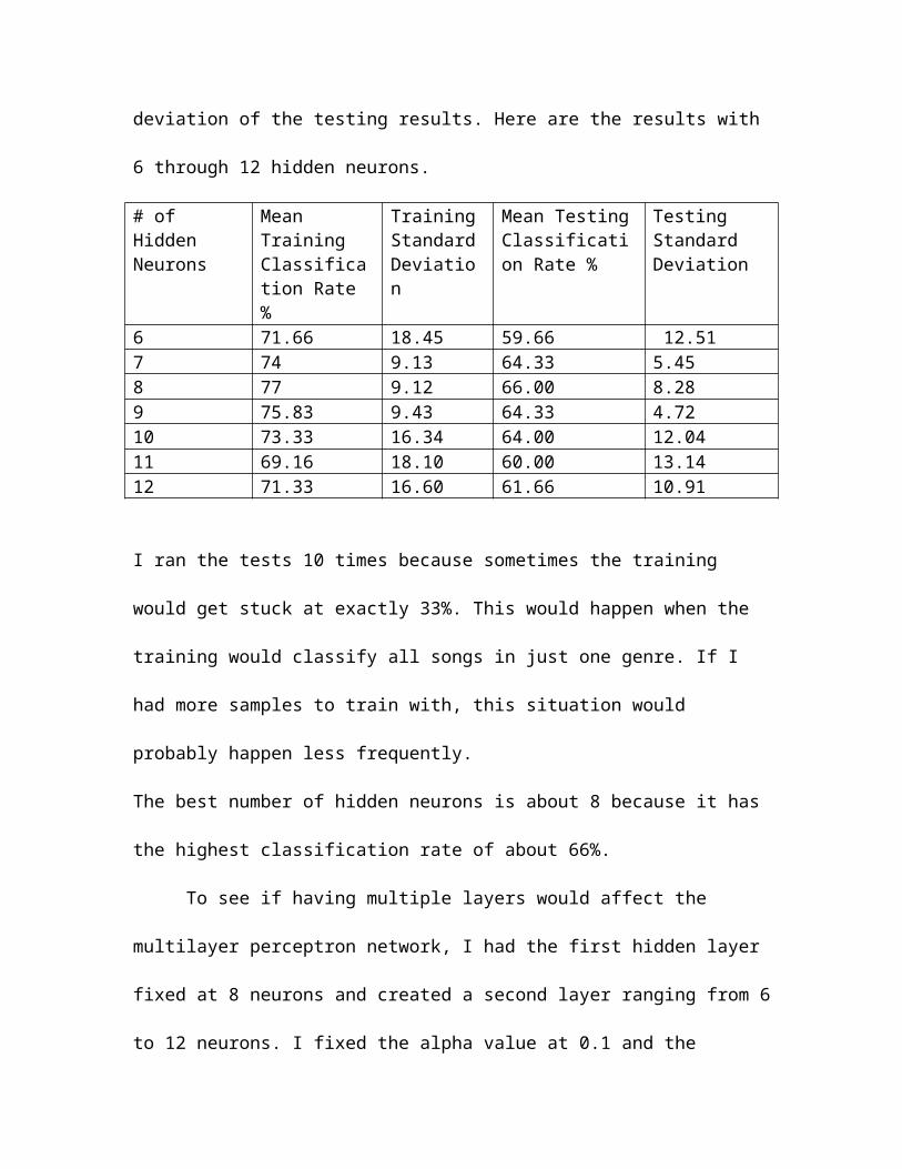
results. Here are the results with 6 through 12 hidden neurons.

# of Hidden Neurons

Mean Training Classification Rate %

Training Standard Deviation

Mean Testing Classification Rate %

Testing Standard Deviation

6 71.66 18.45 59.66 12.517 74 9.13 64.33 5.458 77 9.12 66.00 8.289 75.83 9.43 64.33 4.7210 73.33 16.34 64.00 12.0411 69.16 18.10 60.00 13.1412 71.33 16.60 61.66 10.91

I ran the tests 10 times because sometimes the training would get stuck at exactly 33%.

This would happen when the training would classify all songs in just one genre. If I had

more samples to train with, this situation would probably happen less frequently.

The best number of hidden neurons is about 8 because it has the highest classification

rate of about 66%.

To see if having multiple layers would affect the multilayer perceptron network, I

had the first hidden layer fixed at 8 neurons and created a second layer ranging from 6 to

12 neurons. I fixed the alpha value at 0.1 and the momentum value at 0.8 which are the

default values. I ran each test 10 times and calculated the mean and standard deviation.

# of Hidden Neurons in Second Layer

Mean Training Classification Rate %

Training Standard Deviation

Mean Testing Classification Rate %

Testing Standard Deviation

6 79.33 1.165 68.33 4.777 79.00 1.95 68.66 4.768 77.00 5.76 66.66 4.969 80.50 1.93 67.33 4.09710 76.5 8.10 66 3.4411 75.66 10.31 64.66 10.0812 69.16 15.17 63.33 11.65

Increasing the number of hidden layers from 1 to 2 seemed to improve the results. The

best classification rate increased to 68.66% by adding a hidden layer of 7 neurons. The

results did not improve as much as I thought they would since it still only classifies about

2 out of 3 songs.

With the number of hidden neurons fixed at 8 and with only 1 hidden level, and

the momentum fixed at 0.8, I modified the learning rate, alpha, to go from 0.01, 0.1, 0.2,

0.4 and 0.8. I ran each test 10 times and found the mean and standard deviation.

Alpha value Mean Training Classification Rate %

Training Standard Deviation

Mean Testing Classification Rate %

Testing Standard Deviation

0.01 90.16 2.28 64.66 4.490.1 74.33 13.79 63 10.470.2 39.00 9.26 38 8.770.4 33.33 0.00 33.33 0.000.8 33.33 0.00 33.33 0.00

The classification rate was the best with an alpha value of 0.01. The small learning rate

means that the step size is small so the network is learning a little bit at a time. As the

learning rate increases, the classification rate decreases.

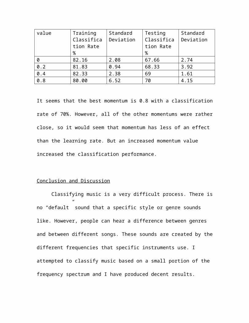
Now to see how changing the momentum value changes the classification rate, I

fixed alpha to the default of 0.1 with 8 hidden neurons and I changed momentum to 0,

0.2, 0.4 and 0.8. The momentum will reduce the gradient change if the gradient changes

violently. It will also increase the change if the gradient keeps going in the same

direction. Again I ran each test 10 times and calculated the mean and standard deviation.

Momentum value

Mean Training Classification Rate %

Training Standard Deviation

Mean Testing Classification Rate %

Testing Standard Deviation

0 82.16 2.08 67.66 2.740.2 81.83 0.94 68.33 3.920.4 82.33 2.38 69 1.610.8 80.00 6.52 70 4.15

It seems that the best momentum is 0.8 with a classification rate of 70%. However, all of

the other momentums were rather close, so it would seem that momentum has less of an

effect than the learning rate. But an increased momentum value increased the

classification performance.

Conclusion and Discussion

Classifying music is a very difficult process. There is no “default” sound that a

specific style or genre sounds like. However, people can hear a difference between genres

and between different songs. These sounds are created by the different frequencies that

specific instruments use. I attempted to classify music based on a small portion of the

frequency spectrum and I have produced decent results.

I originally thought that I would need many features from the frequency domain

to be able to accurately classify music from different genres. However, I did not have

enough samples to fully train a multilayer perceptron network with the number of

features I wanted. Since I had too few training samples, the network would classify all

music in the same genre. If I had more hard drive space and more processing power, I

would have created more samples and I would have increased the number of frequency

bands.

The best multilayer perceptron network configuration which had the highest

classification rate had 1 hidden layer with 8 neurons, a learning value of 0.1 and a

momentum of 0.8. Its classification rate was 70%. Of the 30 test samples, it classified

about 21 songs into the correct genre.

The learning rate seemed to have a negative impact on the classification rate when

it is increased. When the learning rate was increased to 0.4 and 0.8, the mean testing

classification rate decreased to 33%. It seems that the network learned the data better by

learning a little bit at a time. However, the momentum seemed to have a positive impact

on the classification rate. When the momentum was increased to 0.8, the mean testing

classification rate peaked at 70%.

The best performance came with the simplest network. The K-nearest neighbor

with only 6 features using 3-way cross validation was able to get a 73% classification

rate. This surprised me since the K-nearest neighbor should be the base performance

measurement. The multilayer perceptron network was able to double its performance

once the number of features was reduced from 122 to 6.

Unfortunately, my results do not perform as well as others. Shihab Jimaa et. al.

were able to classify music with an accuracy rate as high as 97.6%. They used 170 audio

samples of rock, classical, country, jazz, folk and pop of music recorded at 44.1Khz,

which is CD quality. They were able to randomly select 5 second samples through out the

song and extract their features. They extracted 14 octave values over 3 frequency bands

to get 42 different distribution values. They then used a linear discriminant analysis based

classifier to classify their music. They used digital signal processing techniques that are

more advanced than I have ever worked with so they were able to classify their music

better. However, my technique of sampling the frequency content of the songs was not a

bad attempt since it was able to classify music at a 73% accuracy rate with the simple K-

nearest neighbor network.

References

Alghoniemy, Masoud. Tewfik, Ahmed H. “Rhythm And Periodicity Detection in Polyphonic Music.” Pg 185-190.http://ieeexplore.ieee.org.ezproxy.library.wisc.edu/iel5/6434/17174/00793818.pdf?tp=&arnumber=793818&isnumber=17174

“Audio Topics: The Frequencies of Music” PBS International 633 granite Courthttp://www.psbspeakers.com/audioTopics.php?fpId=8&page_num=1&start=0

Cheng, Kileen. Nazer, Bobak. Uppuluri, Jyoti. Verret, Ryan. “Beat This A Synchronization Project.” http://www.owlnet.rice.edu/~elec301/Projects01/beat_sync/beatalgo.html

Jimaa, Shihab. Krishnan, Sridhar. Umapathy, Karthikeyan. “Multigroup Classification of Audio Signals Using Time-Frequency Parameters.”http://ieeexplore.ieee.org/iel5/6046/30529/01407903.pdf?tp=&arnumber=1407903&isnumber=30529

Zhang, Yibin. Zhou Jie. “A Study Of Content-Based Music Classification.” pg 113-116. Department of Automation, Tsinghua University, Beijing 100084, Chinahttp://ieeexplore.ieee.org.ezproxy.library.wisc.edu/iel5/8675/27495/01224828.pdf?tp=&arnumber=1224828&isnumber=27495

Appendix A: Source Files:

getData.m - This computes all of the data from the sound files listed in the file named

"files". It creates the length, beats per minute and the short time frequency transform on

the songs. It saves the data to "dataFile." This will not work unless you have the wave

files used to collect the data. The name of the input files and the name of the saved output

files were changed from classical, classic rock, and pop.

Stft.m - This computes the FFT of a 5 second sample. It averages the FFT over 250ms

samples.

getSongAndLength.m - This gets the length of the song and the 5 second sample of the

song.

Control.m, filterbank.m, hwindow.m, diffract.m, timecomb.m – All of these files were

written by Kileen Cheng, Bobak Nazer, Jyoti Uppuluri, and Ryan Verret and were used

to get the tempo of the songs.

FeatureReduction.m - This was used to reduce the 122 features down to the most

important features using 3-way cross validation and the KNN.

MakeMLPData.m – This creates the multilayer perceptron data from the reduced

features.

bpAlpha.m and bpconfigAlpha.m – These files were used to test different values of alpha

on the multilayer perceptron network. The results were saved in crateTrainArray and

createTestArray.

bpMom.m and bpconfigMom.m – These files were used to test different values of

momentum on the multilayer perceptron network. The results were saved in

crateTrainArray and createTestArray.

bpHiddenLayers.m and bpconfigHiddenLayers.m – These files were used to test different

number of hidden neurons on the second hidden layer of the multilayer perceptron

network. The results were saved in crateTrainArray and createTestArray.

bpNumberOfHidden.m and bpconfigNumberOfHidden.m – These tests different numbers

of hidden neurons on the first hidden layer of the multilayer perceptron network. The

results were saved in crateTrainArray and createTestArray.

Classicalfiles, classicrockfiles, popfiles – These files list the names of the wave files used

in classical, classic rock and pop.

classicalData, classicRockData, popData – These files contain the 122 features of the 30

different songs in each genre.

mlpTrainData, mlpTestData – These files contain the reduced features of the different

wave files and were used in training and testing the multilayer perceptron network.

All other files were used for the K nearest neighbor network or the multilayer perceprton

network and were written by Professor Yu Hen Hu.

Appendix B: Songs Used

Pop songs:Green Day - American IdiotMatchbox 20 - Real WorldThe Wallflowers - HerosTracy Chapman - Give Me One ReasonAlanis Morissette - You Oughta KnowEric Clapton - Change The WorldThe Killers - Mr BrightsideGoo Goo Dolls - IrisGreen Day - HolidayMatchbox 20 - 3 AM.Sheryl Crow - All I Wanna DoAlanis Morissette - IronicColdplay - Fix YouColdplay - The ScientistGreen Day - Boulevard Of Broken DreamsMadonna - Ray of LightMatchbox 20 - PushThe Killers - Somebody Told MeColdplay - ClocksGorillaz - Clint EastwoodShania Twain – You’re Still The OneColdplay - TroubleGarbage - Stupid GirlGorillaz - Feel Good IncREM - Losing My ReligionColdplay - Speed Of SoundJewel - Who Will Save Your SoulNatalie Imbruglia - TornGreen Day - Wake Me Up When September EndsEric Clapton - My Fathers Eyes

Classic Rock SongsEric Clapton - I Feel FreeJimi Hendrix - Purple HazeLed Zeppelin - Black Dog

Eric Clapton - Sunshine Of Your LoveJimi Hendrix - Hey JoeLed Zeppelin - Rock and RollEric Clapton - White RoomJimi Hendrix - The Wind Cries MaryLed Zeppelin - The Battle of EvermoreEric Clapton - CrossroadsJimi Hendrix - FireLed Zeppelin - Stairway to HeavenEric Clapton - BadgeJimi Hendrix - Highway ChileLed Zeppelin - Misty Mountain HopEric Clapton - Presence Of The LordJimi Hendrix - Are You ExperiencedLed Zeppelin - Four SticksEric Clapton - Blues PowerJimi Hendrix - Burning of the Midnight LampLed Zeppelin - Going to CaliforniaEric Clapton - After MidnightJimi Hendrix - Little WingLed Zeppelin - When the Levee BreaksEric Clapton - Let It RainJimi Hendrix - All Along The WatchtowerEric Clapton - Bell Bottom BluesEric Clapton - LaylaJimi Hendrix - Voodoo Child Slight ReturnEric Clapton - I Shot The Sheriff

Classical SongsAlan Silvestri - Main TitleBeethoven - Symphony No 5 in C minor, Op. 67 , I. Allegro con brioLeonard Bernstein - R. Strauss- Also sprach ZarathustraAlan Silvestri - It's Clara (The Train Part II)Beethoven - Symphony No 5 in C minor, Op. 67 , II. Andante con motoLeonard Bernstein - Bernstein- Overture to CandideAlan Silvestri - Hill ValleyBeethoven - Symphony No 5 in C minor, Op. 67 , III. AllegroLeonard Bernstein - Copland- Hoe-down, Allegro from RodeoAlan Silvestri - The HangingBeethoven - Symphony No 5 in C minor, Op. 67 , IV. AllegroLeonard Bernstein - Smetana- Dance of the Comedians from The Bartered BrideAlan Silvestri - At First SightBeethoven - Overtures , Coriolan, Op. 62Leonard Bernstein - Offenbach- Cancan from Gaite parisienneAlan Silvestri - IndiansBeethoven - Overtures , The Creatures of Prometheus, Op. 43

Leonard Bernstein - Mozart- Overture to The Marriage of FigaroAlan Silvestri - Goodbye ClaraBeethoven - Overtures , Leonore II, Op. 72Leonard Bernstein - Bizet- March of the toreadors from Carmen Suite No. 1Alan Silvestri - Doc ReturnsLeonard Bernstein - Grieg- Norwegian Dance, Op. 35, No. 2Alan Silvestri - Point Of No Return (The Train Part III)Leonard Bernstein - Rimsky-Korsakov- Dance fo the Tumblers from The Snow MaidenAlan Silvestri - The Future Isn't WrittenLeonard Bernstein - Tchaikovsky- Russian Dance (Trepak) from The NutcrackerAlan Silvestri - The ShowdownLeonard Bernstein - Humperdinck- Children's Prayer from Hansel und GretelAlan Silvestri - Doc To The Rescue