Classification of Wetlands and Analysis of Wetlands ... · PDF fileClassification of Wetlands...
28
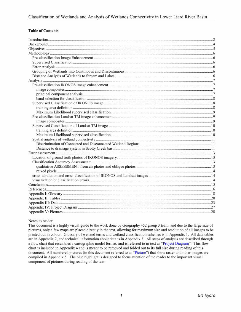
Classification of Wetlands and Analysis of Wetlands Connectivity in Lower Liard River Basin 1 GIS Hydro Table of Contents Introduction ......................................................................................................................................................................2 Background ......................................................................................................................................................................4 Objectives ........................................................................................................................................................................5 Methodology ....................................................................................................................................................................6 Pre-classification Image Enhancement ........................................................................................................................6 Supervised Classification .............................................................................................................................................6 Error Analysis ..............................................................................................................................................................6 Grouping of Wetlands into Continuous and Discontinuous .........................................................................................6 Distance Analysis of Wetlands to Stream and Lakes ...................................................................................................6 Analysis ...........................................................................................................................................................................7 Pre-classification IKONOS image enhancement .........................................................................................................7 image composites .....................................................................................................................................................7 principal component analysis ...................................................................................................................................7 band selection for classification ...............................................................................................................................8 Supervised Classification of IKONOS image ..............................................................................................................8 training area definition .............................................................................................................................................8 Maximum Likelihood supervised classification.......................................................................................................9 Pre-classification Landsat TM image enhancement .....................................................................................................9 image composites .....................................................................................................................................................9 Supervised Classification of Landsat TM image .......................................................................................................10 training area definition ...........................................................................................................................................10 Maximum Likelihood supervised classification.....................................................................................................10 Spatial analysis of wetland connectivity ....................................................................................................................11 Discrimination of Connected and Disconnected Wetland Regions........................................................................11 Distance to drainage system in Scotty Creek basin ................................................................................................11 Error assessment ............................................................................................................................................................13 Location of ground truth photos of IKONOS imagery: .............................................................................................13 Classification Accuracy Assessment:.........................................................................................................................13 qualitative ASSESSMENT from air photos and oblique photos............................................................................13 mixed pixels ...........................................................................................................................................................14 cross-tabulation and cross-classification of IKONOS and Landsat images ...............................................................14 visualization of classification errors...........................................................................................................................14 Conclusions ....................................................................................................................................................................15 References ......................................................................................................................................................................16 Appendix І: Glossary .....................................................................................................................................................18 Appendix ІI: Tables .......................................................................................................................................................20 Appendix ІII: Data .........................................................................................................................................................23 Appendix ІV: Project Diagram ......................................................................................................................................27 Appendix V: Pictures .....................................................................................................................................................28 Notes to reader: This document is a highly visual guide to the work done by Geography 452 group 3 team, and due to the large size of pictures, only a few maps are placed directly in the text, allowing for maximum size and resolution of all images to be printed out in colour. Glossary of wetland terms and wetland classification schemes is in Appendix 1. All data tables are in Appendix 2, and technical information about data is in Appendix 3. All steps of analysis are described through a flow chart that resembles a cartographic model format, and is referred to in text as “Project Diagram”. This flow chart is included in Appendix 4 and is meant to be removed and folded out to its full size during reading of this document. All numbered pictures (in this document referred to as “Picture”) that show raster and other images are compiled in Appendix 5. The blue highlight is designed to focus attention of the reader to the important visual component of pictures during reading of the text.
-
Upload
nguyendieu -
Category
Documents
-
view
244 -
download
1
Transcript of Classification of Wetlands and Analysis of Wetlands ... · PDF fileClassification of Wetlands...
Classification of Wetlands and Analysis of Wetlands Connectivity in Lower Liard River Basin
1 GIS Hydro
Table of Contents Introduction......................................................................................................................................................................2 Background ......................................................................................................................................................................4 Objectives ........................................................................................................................................................................5 Methodology....................................................................................................................................................................6
Pre-classification Image Enhancement ........................................................................................................................6 Supervised Classification .............................................................................................................................................6 Error Analysis ..............................................................................................................................................................6 Grouping of Wetlands into Continuous and Discontinuous.........................................................................................6 Distance Analysis of Wetlands to Stream and Lakes...................................................................................................6
Analysis ...........................................................................................................................................................................7 Pre-classification IKONOS image enhancement .........................................................................................................7
image composites.....................................................................................................................................................7 principal component analysis ...................................................................................................................................7 band selection for classification ...............................................................................................................................8
Supervised Classification of IKONOS image ..............................................................................................................8 training area definition .............................................................................................................................................8 Maximum Likelihood supervised classification.......................................................................................................9
Pre-classification Landsat TM image enhancement.....................................................................................................9 image composites.....................................................................................................................................................9
Supervised Classification of Landsat TM image .......................................................................................................10 training area definition ...........................................................................................................................................10 Maximum Likelihood supervised classification.....................................................................................................10
Spatial analysis of wetland connectivity ....................................................................................................................11 Discrimination of Connected and Disconnected Wetland Regions........................................................................11 Distance to drainage system in Scotty Creek basin................................................................................................11
Error assessment ............................................................................................................................................................13 Location of ground truth photos of IKONOS imagery: .............................................................................................13 Classification Accuracy Assessment:.........................................................................................................................13
qualitative ASSESSMENT from air photos and oblique photos............................................................................13 mixed pixels ...........................................................................................................................................................14
cross-tabulation and cross-classification of IKONOS and Landsat images ...............................................................14 visualization of classification errors...........................................................................................................................14
Conclusions....................................................................................................................................................................15 References......................................................................................................................................................................16 Appendix І: Glossary .....................................................................................................................................................18 Appendix ІI: Tables .......................................................................................................................................................20 Appendix ІII: Data .........................................................................................................................................................23 Appendix ІV: Project Diagram ......................................................................................................................................27 Appendix V: Pictures .....................................................................................................................................................28 Notes to reader: This document is a highly visual guide to the work done by Geography 452 group 3 team, and due to the large size of pictures, only a few maps are placed directly in the text, allowing for maximum size and resolution of all images to be printed out in colour. Glossary of wetland terms and wetland classification schemes is in Appendix 1. All data tables are in Appendix 2, and technical information about data is in Appendix 3. All steps of analysis are described through a flow chart that resembles a cartographic model format, and is referred to in text as “Project Diagram”. This flow chart is included in Appendix 4 and is meant to be removed and folded out to its full size during reading of this document. All numbered pictures (in this document referred to as “Picture”) that show raster and other images are compiled in Appendix 5. The blue highlight is designed to focus attention of the reader to the important visual component of pictures during reading of the text.

Classification of Wetlands and Analysis of Wetlands Connectivity in Lower Liard River Basin
2 GIS Hydro
Introduction The Global Energy and Water Cycle Experiment (GEWEX) is a program initiated by the World Climate Research Program (WCRP) to observe, understand, and model the hydrological cycle and energy fluxes in the atmosphere, at land surface, and in the upper oceans. GEWEX is an integrated program of research, observations, scientific activities and the application of remote sensing technology to model regional hydrological processes and water resources. In conjunction with the GEWEX Continental-scale International Project (GCIP) in the Mississippi Basin, the Canadian contribution to GEWEX, the Mackenzie GEWEX Study (MAGS), conducted a series of large-scale hydrological studies within the Mackenzie River Basin. The central objective of MAGS is to develop a research methodology to model water and energy fluxes for a characteristic Canadian Arctic Basin (Pietroniro et al, 1996a). The Liard River Valley is a large wetland-dominated sub-basin of the Mackenzie River Basin. This sub-basin has been selected as a research watershed representative of the wetland-dominated zone of discontinuous permafrost. The sub-basin can be further partitioned into six catchment areas that include: the Martin River, the Blackstone River, the Birch River, the Poplar River, the Jean Marie River, and the Scotty Creek catchment (a map that is shown on title page). The detailed analysis of flow pathways through wetland areas requires large-scale analysis of representative catchment regions. Consequently, project research initiates with the large-scale analysis of Scotty Creek, and then proceeds to the extrapolation of information for subsequent application to the analysis of the entire Lower Liard River Valley. Research interests function to determine the unique combination of hydrological variables such as rainfall, soil moisture, snow cover, lake, ice, and glacier evaporation, and hydrologically significant terrain mapping to facilitate an increased understanding and prediction of energy flux (Quinton et al, 2000).
Figure 1 Location of lower Liard River and Scotty Creek basin area in the NWT.
Classification of Wetlands and Analysis of Wetlands Connectivity in Lower Liard River Basin
3 GIS Hydro
Classification of Wetlands and Analysis of Wetlands Connectivity in Lower Liard River Basin
4 GIS Hydro
Background Glaciers helped to form the wetlands in Canada 9,000 to 12,000 years ago. Large wetlands formed when glaciers dammed rivers, scoured valleys, and reworked floodplains. Countless smaller wetlands were created as a result of large blocks of ice left behind by receding glaciers that formed pits and depressions in the land surface. Numerous depressions later filled with water due to poor drainage or intersection with the water table. Of recent interest in society is the relationship between the health of wetland regions and the human value obtained from them. Wetlands are considered one of the most productive ecosystems on earth. Such regions regulate water levels within watersheds, improve water quality, reduce flood and storm damages, provide important fish and wildlife habitat, as well as support hunting, fishing, and other recreational activities. Wetlands are important features in watershed management (Goldberg, 2000). Regions inundated with water almost year round are termed wetlands. Ecosystems that develop on these lands subsequently are dominated by the presence of water excesses. Wetlands are found within flat vegetated areas, landscape depressions, as well as between water and dry land proximal to the edges of streams, rivers, lakes, and coastlines. The recurrent or prolonged presence of water at or near surface is the dominant factor determining the nature of soil development and the types of plant and animal communities living in the soil and on its surface (NWWG, 1988). Classification of wetlands environments can then be undertaken by the presence of unique vegetation termed hydrophytes that are adapted to life in soils that form under flooded or saturated conditions.
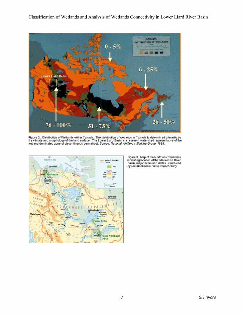
Wetlands occupy extensive regions of Canada. A significant proportion of these wetlands have been anthropogenically altered, some exploited for peat others drained for agricultural or forestry applications. The extent of wetlands in Canada is not known with any degree of accuracy. The distribution of wetlands in Canada is determined primarily by the climate and by the morphology of the land surface, alone or in combination. Climate functions to determine the volume of water a region receives through precipitation. Incoming energy plays an important role in the fate of the precipitated water lower incoming radiation rates generate a lower evapotransporation rate, consequently allowing water to pool on the surface. Figure 3 shows wetland distribution in Canada Land morphology acts to influence the distribution of surplus water and the ultimate location of wetlands. Large, flat plains of fine-textured soils have the intrinsic property of poor internal and external drainage rates that result in surface water surplus. Within undulating surface topography wetlands may form in small, poorly drained depressions. In cool areas with low rainfall, wetlands usually develop only in depressions where water collects from adjacent slopes or from the upstream part of a catchment basin. Water may also be added to the system through groundwater discharge. In addition to climate and the surface configuration of the land, the physical and mineralogical characteristics of surface materials also influence wetland development. The texture of the surface material
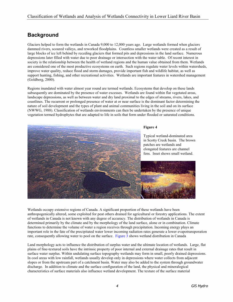
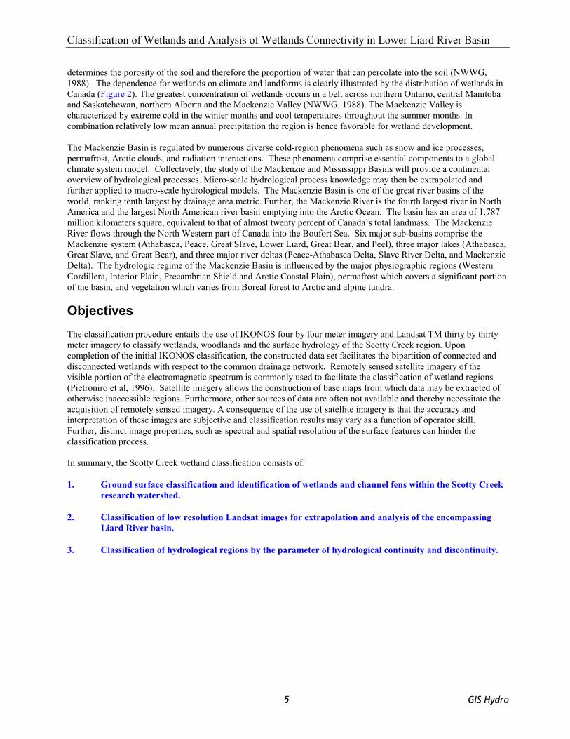
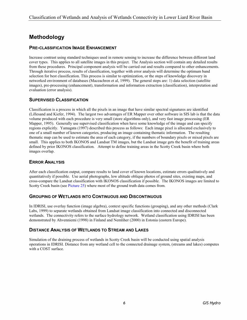
Figure 4 Typical wetland-dominated area in Scotty Creek basin. The brown patches are wetlands and elongated features are channel fens. Inset shows small wetland.
Classification of Wetlands and Analysis of Wetlands Connectivity in Lower Liard River Basin
5 GIS Hydro
determines the porosity of the soil and therefore the proportion of water that can percolate into the soil (NWWG, 1988). The dependence for wetlands on climate and landforms is clearly illustrated by the distribution of wetlands in Canada (Figure 2). The greatest concentration of wetlands occurs in a belt across northern Ontario, central Manitoba and Saskatchewan, northern Alberta and the Mackenzie Valley (NWWG, 1988). The Mackenzie Valley is characterized by extreme cold in the winter months and cool temperatures throughout the summer months. In combination relatively low mean annual precipitation the region is hence favorable for wetland development. The Mackenzie Basin is regulated by numerous diverse cold-region phenomena such as snow and ice processes, permafrost, Arctic clouds, and radiation interactions. These phenomena comprise essential components to a global climate system model. Collectively, the study of the Mackenzie and Mississippi Basins will provide a continental overview of hydrological processes. Micro-scale hydrological process knowledge may then be extrapolated and further applied to macro-scale hydrological models. The Mackenzie Basin is one of the great river basins of the world, ranking tenth largest by drainage area metric. Further, the Mackenzie River is the fourth largest river in North America and the largest North American river basin emptying into the Arctic Ocean. The basin has an area of 1.787 million kilometers square, equivalent to that of almost twenty percent of Canada’s total landmass. The Mackenzie River flows through the North Western part of Canada into the Boufort Sea. Six major sub-basins comprise the Mackenzie system (Athabasca, Peace, Great Slave, Lower Liard, Great Bear, and Peel), three major lakes (Athabasca, Great Slave, and Great Bear), and three major river deltas (Peace-Athabasca Delta, Slave River Delta, and Mackenzie Delta). The hydrologic regime of the Mackenzie Basin is influenced by the major physiographic regions (Western Cordillera, Interior Plain, Precambrian Shield and Arctic Coastal Plain), permafrost which covers a significant portion of the basin, and vegetation which varies from Boreal forest to Arctic and alpine tundra. Objectives The classification procedure entails the use of IKONOS four by four meter imagery and Landsat TM thirty by thirty meter imagery to classify wetlands, woodlands and the surface hydrology of the Scotty Creek region. Upon completion of the initial IKONOS classification, the constructed data set facilitates the bipartition of connected and disconnected wetlands with respect to the common drainage network. Remotely sensed satellite imagery of the visible portion of the electromagnetic spectrum is commonly used to facilitate the classification of wetland regions (Pietroniro et al, 1996). Satellite imagery allows the construction of base maps from which data may be extracted of otherwise inaccessible regions. Furthermore, other sources of data are often not available and thereby necessitate the acquisition of remotely sensed imagery. A consequence of the use of satellite imagery is that the accuracy and interpretation of these images are subjective and classification results may vary as a function of operator skill. Further, distinct image properties, such as spectral and spatial resolution of the surface features can hinder the classification process. In summary, the Scotty Creek wetland classification consists of: 1. Ground surface classification and identification of wetlands and channel fens within the Scotty Creek
research watershed.
2. Classification of low resolution Landsat images for extrapolation and analysis of the encompassing Liard River basin.
3. Classification of hydrological regions by the parameter of hydrological continuity and discontinuity.
Classification of Wetlands and Analysis of Wetlands Connectivity in Lower Liard River Basin
6 GIS Hydro
Methodology PRE-CLASSIFICATION IMAGE ENHANCEMENT Increase contrast using standard techniques used in remote sensing to increase the difference between different land cover types. This applies to all satellite images in this project. The Analysis section will contain any detailed results from these procedures. Principal component analysis will be carried out and results compared to other enhancements. Through iterative process, results of classification, together with error analysis will determine the optimum band selection for best classification. This process is similar to optimization, or the steps of knowledge discovery in networked environment of databases (Maceachren et al, 1999). The general steps are: 1) data selection (satellite images), pre-processing (enhancement), transformation and information extraction (classification), interpretation and evaluation (error analysis). SUPERVISED CLASSIFICATION Classification is a process in which all the pixels in an image that have similar spectral signatures are identified (Lillesand and Kiefer, 1994). The largest two advantages of ER Mapper over other software in SIS lab is that the data volume produced with each procedure is very small (store algorithms only), and very fast image processing (ER Mapper, 1995). Generally use supervised classification when have some knowledge of the image and can specify regions explicitly. Yamagata (1997) described this process as follows: Each image pixel is allocated exclusively to one of a small number of known categories, producing an image containing thematic information. The resulting thematic map can be used to estimate the area of each category, if the numbers of boundary pixels or mixed pixels are small. This applies to both IKONOS and Landsat TM images, but the Landsat image gets the benefit of training areas defined by prior IKONOS classification. Attempt to define training areas in the Scotty Creek basin where both images overlap. ERROR ANALYSIS After each classification output, compare results to land cover of known locations, estimate errors qualitatively and quantitatively if possible. Use aerial photographs, low altitude oblique photos of ground sites, existing maps, and cross-compare the Landsat classification with IKONOS classification if possible. The IKONOS images are limited to Scotty Creek basin (see Picture 25) where most of the ground truth data comes from. GROUPING OF WETLANDS INTO CONTINUOUS AND DISCONTINUOUS In IDRISI, use overlay function (image algebra), context specific functions (grouping), and any other methods (Clark Labs, 1999) to separate wetlands obtained from Landsat image classification into connected and disconnected wetlands. The connectivity refers to the surface hydrology network. Wetland classification using IDRISI has been demonstrated by Ahvenniemi (1998) in Finland and Nemliher (2000) in Estonia (eastern Europe). DISTANCE ANALYSIS OF WETLANDS TO STREAM AND LAKES Simulation of the draining process of wetlands in Scotty Creek basin will be conducted using spatial analysis operations in IDRISI. Distance from any wetland cell to the connected drainage system, (streams and lakes) computes with a COST surface.

Classification of Wetlands and Analysis of Wetlands Connectivity in Lower Liard River Basin
7 GIS Hydro
Analysis PRE-CLASSIFICATION IKONOS IMAGE ENHANCEMENT Given that this project relies on digital satellite imagery, the quality of the first step of image enhancement is critical to the following analysis (Richards, 1986). The following discussion applies to both the IKONOS and Landsat TM images, although the latter has more additional bands and has lower resolution. It is an integral part of this project and provides much basic information required to understand the classification results and spatial analysis that follows. Our attempt is to describe the landscapes as much as possible, to justify the selection of classes later on. IMAGE COMPOSITES The four spectral bands of IKONOS image (1 blue, 2 green, 3 red, 3 near infrared), each contribute differently to the discrimination of the land features. Examples are shown in Picture 2. Blue band has relatively low contrast, is affected by haze, and almost any dry area such as moss mats, dry grass, deciduous forests, will appear bright. Green band has good contrast between green-looking vegetation and areas that reflect highly in other “colours”. The light-green leafed deciduous trees appear brighter than darker green coniferous trees. The best contrast between channel fens, forests, and wetlands is in red band. The drier wetlands with yellow to orange coloured moss mats are also bright in red band because they are high in red reflectivity. Healthy vegetation absorbs red light preferentially, so it will look darker on this image, so density of coniferous stands inversely related to brightness in this band (more red wavelength absorption by leaves). What is interesting here, the deciduous trees are changing leaf colours, so more red light is reflected as a result of decreased photosynthesis but also as a result of colour change. The same holds for drying mosses and shrubs, which give some wetlands different appearance. Finally, the near-infrared band image has bright pixels where there is healthy vegetation cover that reflects highly in this part of spectrum. In contrast, any wet areas with standing water will be much darker because infra-red light is greatly absorbed by water. Normally, the near-IR band can easily distinguish between wetlands and other land features (Anderson & Perry, 1996). In our study area the wetlands in late summer consist mostly of floating moss and grass that are highly productive, very little open water in the wetlands, thus appearing much like healthy grass or similar vegetation. Thus, infrared band alone is not sufficient to separate wetlands from other landscapes in this area. The colour composite of the first three bands (Picture 2) helps to identify the landscapes in true colour (similar to a colour photo) image. The data is now manipulated for each band separately to increase the contrast among different features to help with identification. Some of the distinguishable land cover types are lakes, channel fens, small wetlands, coniferous forests, deciduous forests, and transitional vegetated areas (Pictures 5 and 6). Following textbook methodology (Lillesand and Kiefer, 1994), this involves change of input limits to span the frequency histogram for each band to eliminate spurious data (clipping of histogram), and contrast stretch using linear transform with level slicing until the features of wetlands, and forests have the highest contrast possible at large scale and at the scale of whole image. As an example, Picture 3 and 4 compare two colour composites of the same area near a small lake a few hundred meters across, one enhanced and one not. The true colour visible spectrum image shows a small lake (black), channel fens (brown-green, sinuous, look like channels) and small islands of sparse or transitional coniferous forest (green) and small patches of wetlands (orange - yellow), dense coniferous stands (dark green) and large patches of deciduous forest (light green). The enhanced image clearly differentiates between all these features. The coniferous forested areas are green or dark green, channel fens or fens are orange (with brown patches where ponds and open water occur), dry wetlands are purple, and deciduous trees are yellow-green. The lake is also black in colour. A low-pass filter was applied to smooth out the features. PRINCIPAL COMPONENT ANALYSIS Another enhancement method that was used is the Principal Component Analysis (Richards, 1984). This statistical procedure reduces redundancy in multispectral image data (many features reflect similarly in several bands). Each of the principal components can be treated as a single band, and then combined into colour composite image (Picture 8). The colour is false because the image is statistical and colour assignment is arbitrary. Each of the components conveys unique information about the landscape (Picture 11), and the last component usually has the most
Classification of Wetlands and Analysis of Wetlands Connectivity in Lower Liard River Basin
8 GIS Hydro
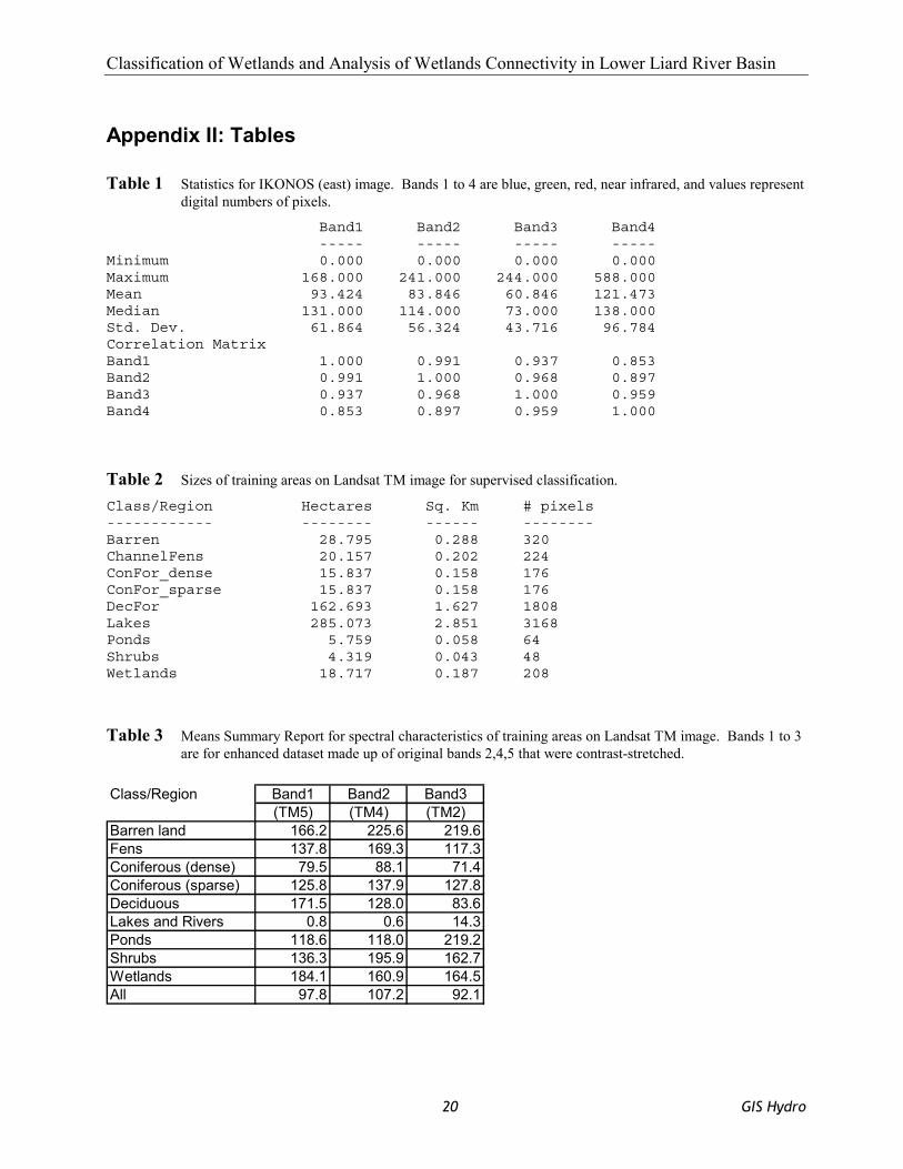
background noise. The standard enhancement procedures follow. The results in Picture 8 show the central section of IKONOS (east) image, with Goose Lake to the south and smaller lakes around it. Channel fens, shown in light blue, are distinct from all other features. Wetlands and forests are also well differentiated. Of the 4 principal components, only the first 3 are used in this colour composite. Colour assignment is red, green, and blue for principal components 1, 2, and 3. For example, the 4th principal component has much noise but it separates the deciduous forests from other features, and all wet areas among wetlands are separated. The 3rd principal component separates the channel fens and distinguishes between deep and shallow lake water. The 1st and 2nd principal components look similar to visible spectrum bands of that image, and the 1st one has the most contrast. BAND SELECTION FOR CLASSIFICATION Overall, the principal components were selected for further analysis. The original four bands are highly correlated (Table 1). The principal component will have the least correlation and redundancy. The entire Scotty Creek basin is covered by two IKONOS images, here called “east” and “west” (Pictures 9 and 10). Even after all enhancement attempts, the “west” image contained too much cloud cover with cloud shadows, and atmospheric haze which prevented adequate contrast between landscape cover types. This image was removed from further analysis. The proper choice of band combination and enhancement is an iterative process linked with results of classification (see project diagram), and follows work of Wakelyn (1990), Pietroniro et al (1996b), Hoffbeck et al (1996) and remote sensing reference (Richards, 1986). The next section describes classification results, but it’s important to note that it was performed several times using different band combinations. The best results were obtained from principal components because the subsequent supervised classification of this IKONOS image had problems separating deciduous forests from dry wetlands using enhanced bands 1 through 4. Therefore, it was abandoned when the principal component analysis showed better results. The following section describes in detail the classification accuracy assessment methods. SUPERVISED CLASSIFICATION OF IKONOS IMAGE TRAINING AREA DEFINITION Supervised classification starts with "training" regions drawn on the image. These areas must be very homogeneous and represent only one land cover type (Lillesand and Kiefer, 1994). The photographs of ground sites (Quinton pers. comm) from colour low altitude oblique photos provide very limited ground truth for the purpose of creating training areas. The methodology adopted originally for this project required that training areas be located in the IKONOS image classification be trained in known locations where land cover type is visible on existing photographs (Picture 15) in the Scotty Creek basin. Each site has GPS coordinates (see Appendix 3) that can be located on the satellite image, but due to heterogeneity of terrain (many small wetland and forest patches) and inaccuracy of the ground sites (within 100 m), many of the sites could not be accurately located on the IKONOS image. For one good example, see Picture 6. Black and white aerial photographs were also used to verify classification results (Picture 17), but error analysis is described in a separate section. The imagery was spot checked at various locations and the image class was compared to the forest cover map. An error assessment was performed on the classification. Although efforts have been made to make this classification as accurate as possible, there is bound to be some confusion between classes (see section on Error Analysis). Enhanced images were compared with panchromatic photography of the Scotty Creek basin to determine common surface features. Further enhancements were conducted on images with poor feature recognition resolutions. Images that possessed definite feature recognition were used in the classification process. As a consequence of the project objectives of wetland classification and their connection to a common stream network, the surface cover was divided into general classes: Coniferous Forest, Deciduous Forest, Channel Fen, Wetland, Lakes, other land cover The process of supervised classification allocates each image pixel exclusively to one of a small number of known categories thus constructing an image containing surface feature thematic information. Representative surface feature pixels were selected to prototype each of the outlined sets of classes. Selected pixels comprise the training data set. Each training data set comprises a training site or polygon for a defined surface class. Training data is used to

Classification of Wetlands and Analysis of Wetlands Connectivity in Lower Liard River Basin
9 GIS Hydro
estimate the parameters of a particular classifier algorithm. Determined parameters are applied to a probability model and enable the construction of mathematical equations which partition of the electromagnetic spectrum in a one to one correspondence with the selected surface feature class. The set of parameters for a given class is termed the signature of that class. Picture 12 describes the training polygons drawn on IKONOS images in ER Mapper software. Spectral cluster analysis (or scattergram) was used to evaluate the selection of training sites with respect to surface class selection without ambiguity (Picture 13). For cases in that spectral distinction between surface classes were adequate the training sites were used for the classification process. Further polygons were selected for cases in which classes failed to meet the criteria. The scattergrams are linked to interactive editing of the training areas and change accordingly. When four bands are used in classification, the scattergram of all four has four dimensions. Here, four two-dimensional plots are shown instead. Without going into details, the spectral responses of each class of training areas is represented by an ellipse (colour coded by class type), which is plotted on equally scaled axes, one for each band. The axes are all scaled 0 to 255 (for 8 bit digital numbers of pixels). The data extent is plotted as grey scatterplot. The black large ellipse is the mean response of all training areas. The deciduous forests (bright green) are very bright and clearly separate in all scattergrams. Water classes have low digital numbers and also separate. Other classes separate well only in plot of 1st and 3rd principal component spectral bands. The class “wetlands” separates better than class “fens”, which is more likely to be misclassified with forests than “wetlands”. Overall, the more crowded and overlapping the ellipses, the less distance between means of the spectral signatures and more confusion results during classification. MAXIMUM LIKELIHOOD SUPERVISED CLASSIFICATION It is the most common supervised classification method. When the distributions of the spectra are normal, theory predicts that this method will give the best results (Arai, 19921), (Yamagata, 1997), (Richards, 1984). The classification colours for any classification in this project are given in map legend of Picture 16, which presents thematic map of east side of Scotty Creek basin based on IKONOS image supervised classification. The results of IKONOS image classification show good correspondence between landscapes. In Picture 14, a section of the image is compared between classification results, true colour composite (visible spectrum), and false colour composite made of principal components. Channel fens are clearly delineated, forest patches and small wetlands are correctly classified (see zoom-in of the same view on Picture 14). Due to lack of ground truth, the error analysis is only qualitative but shows satisfactory classification accuracy (see section on Error analysis). The Scotty Creek basin (Picture 16) consists of a network of channel fens that connect lakes and streams and extend the drainage network during spring snow melt period in the arctic (Quinton et al, 2000). There is also a large number of scattered wetlands that have different spectral characteristics than the channel fens. The coniferous tree cover ranges from dense to sparse, with densest stands grouped into large forest patches. The shrubs and sparse coniferous trees grow between wetlands and form a complex pattern. The classified image was transformed to IDRISI raster format and saved for further analysis of spatial patterns and connectivity. PRE-CLASSIFICATION LANDSAT TM IMAGE ENHANCEMENT The methodology is very similar to the previously discussed IKONOS image. Refer to the Project Diagram for complete description of steps. Here, only notable differences between the IKONOS and Landsat image enhancement and classification are discussed. IMAGE COMPOSITES The standard visible light true colour composite is shown in Picture 22. The scene is very green where vegetation cover dominates and brown where there are wetlands and barren ground. Lakes appear as black spots and rivers are light-toned due to reflection of sunlight. The first four bands from Blue to near Infra-red look similar to those of IKONOS. Bands 5 and 7 extend further into the infrared part of the spectrum (see Picture 19 for images of 6 Landsat bands). At this scale, there is more landscape heterogeneity, except the two large rivers. The false colour composite that uses two visible spectrum bands and one infrared band highlights healthy vegetation in red tones (Picture 20).

Classification of Wetlands and Analysis of Wetlands Connectivity in Lower Liard River Basin
10 GIS Hydro
The NDVI (Normalized Difference Vegetation Index) ratio also highlights vegetation, but has more contrast between different types of vegetation (Lillesand and Kiefer, 1994). Both of these images show the same patterns in vegetation. At this scale wetlands are difficult to identify. Following the work of Wakelyn (1990), band 4 and 5 were contrast stretched with a power curve, and band 2 had a linear stretch. The false colour composite that results from these particular enhancements is shown in Picture 23 (and below). The colours are different here. The orange shades are deciduous forests. Rivers and Lakes are in blue tones. Dense coniferous forests are shown as dark green, but sparse coniferous stands and mixed or immature forests are lighter values of green. These blend into light green coloured fens and wetlands. Barren land is shown as almost white in colour. This image forms the basis of classification. SUPERVISED CLASSIFICATION OF LANDSAT TM IMAGE TRAINING AREA DEFINITION As a point of initiation, a geo-referenced link between the IKONOS imagery and the Landsat imagery was created. The linkage of the imagery enabled the extraction of correctly geo-referenced information from the IKONOS image for use in classification of the Landsat image. Low-altitude oblique colour photography and the previously classified IKONOS image formed the basis information used in Landsat training site identification (Picture 28). The Landsat image covers a much larger area and includes far fewer classes than IKONOS imagery (Picture 25). McNairn (1993) concluded that, as spatial resolution decreases, a wider range of land covers is included in each class. In addition, the variability in spectral values within these broader classes generally increases. As for IKONOS, scattergrams justified the training sites in the Landsat image (see Pictures 29 and 30 for scattergrams). Each scattergram displays the distribution of pixels in a training area in relation to spectral reflectance values for paired Landsat band comparison. In general, wetlands and fens have significant overlap with forests on these diagrams, so significant classification errors are expected. The sizes of training areas were initially small. The training polygons were drawn only in the small section of Scotty Creek basin. After several iterations, the optimal classification required much larger variety of training areas, including some areas outside of Scotty Creek basin and the IKONOS image coverage. Table 4 lists the distances between means of spectral characteristics of the various classes based on training areas. It is in a form of matrix. All numbers are relative, where 0 represents identical training area characteristics, and 20 or higher represent very large difference. The ellipses shown on scattergrams have indicated centers. The difference between these centers is the same as the distance between means. Lakes and rivers are very dissimilar from any other feature, and are expected to be classified correctly. Wetlands are relatively distict from coniferous forests, but are similar to Fens. Sparse coniferous tree patches and channel fens are very likely to be confused during classification. Shrubs may also be confused with Fens (small distance between means). Table 5 shows the same type of information but for training areas improved by addition of areas outside Scotty Creek basin. Overall, the distances between means are larger so less confusion is expeced from classification. The relative brightness of each class of feature in each of the three spectral bands selected for classification (TM5, TM4, TM3 bands) are listed in Table 3. Maximum brightness is at 255, so the smaller the number the darker the feature in that particular band. MAXIMUM LIKELIHOOD SUPERVISED CLASSIFICATION The supervised classification method was used to construct the ground cover image of Liard River region that includes the Scotty Creek study area. The accuracy of the classified images of IKONOS and Landsat were evaluated with panchromatic aerial photography and low-altitude oblique colour photography. The classification of the Landsat imagery was subsequently evaluated with respect the constructed classified IKONOS image. Wakelyn (1990) demonstrated the use of Landsat imagery to classify wetlands in Northwest Territories to a degree of accuracy estimated from 67% to 89%, but error analysis sections shows that our classification is less accurate at about 50% (see Table 7 and section on Error analysis). The resulting classified Landsat TM image of lower Liard River basin is printed in Picture 36, and Picture 41 (with legend). The colour scheme is the same as for all previous classifications. The orange-coloured fens and yellow-coloured wetlands form large percentage of land-cover south of the Mackenzie River. The most prevalent land cover

Classification of Wetlands and Analysis of Wetlands Connectivity in Lower Liard River Basin
11 GIS Hydro
class is the coniferous forest. Deciuous forests are common in many areas as compared to Scotty Creek basin, which had very few deciduous stands. Error analysis will show that “fens” and “wetlands” are difficult to distinguish because each may have similar reflectances in the same spectral bands. Pietroniro et al (1996a) used Landsat TM image classification and obtained the following results in percentage of area classified (note that class definitions are different): water (2 %), wetlands (22%), transitional and dense coniferous forest (45%), mixed forest (17%), deciduous forest (11%), shrubs (1%). The class/area summary from this project in Table 6 indicates that the two landscapes are not the same, but the magnitudes of areas classified by land cover type are similar. SPATIAL ANALYSIS OF WETLAND CONNECTIVITY The different characteristics of spatial patterns of wetlands and other water storages strongly influence flow paths in drainage networks. The proper representation of connectivity can be critically important for hydrologic runoff predictions (Western et al, 2001). The objective to distinguish between connected and disconnected wetlands (i.e. connection to the draining system) was conducted with spatial analysis in IDRISI. The use of satellite images for classification of Scotty Creek made it an easy choice between vector and raster format. Raster-based systems are compatible with the data produced by satellite-based sensors, and photographs. These systems produce imagery in raster form comprising a rectangular array of pixels, which is then analyzed and stored to create a grid map. Raster data may not explicitly represent feature boundaries but instead uses a stair-stepped appearance (Lyon et al, 1995). Additionally Liard river basin describes an area of continuous fields with unclear boundaries, which is commonly used in the landscape model of raster format, in contrast to the object model, represented by crisply ‘points’, ‘lines’ and ‘areas’. We used IDRISI, which apply the raster model, to detect spatial pattern and obtain spatial information as distance between areas and features. A boundary analysis of the wetlands allow us to exploit the dynamic nature by investigating fields where variables change gradually or represent edges of heterogeneous areas. Analyses of these unclear boundaries play a significant role in advancing our understanding of the relationships underpinning the studies of ecological systems and the diverse scientific fields subsumed within them, as hydrology (Jacquez et al, 1999). DISCRIMINATION OF CONNECTED AND DISCONNECTED WETLAND REGIONS The classified Landsat image was used as the source of information, considered the wetlands in Scotty Creek, to make the image more manageable. The boundaries for the Scotty Creek basin was imported from shape file format (ArcView) and rasterised to isolate the Scotty Creek basin in the Landsat image. The area was reclassed into a Boolean image, were the water bodies (wetlands, lakes, ponds and fens) was separated from other land covers. Western et al (2001) used an approach where an algorithm is used to check for any neighbors that are of same value as any other neighbor, row-by-row. This approach is similar to the Group module used by IDRISI, which we find appropriate for this spatial pattern recognition or connectivity (Picture 39). The Group module creates polygons with connecting cells of same classes. To separate the wetland/water body polygons from other land covers, and the image was overlayed with a Boolean image of just wetlands and water bodies. Using a statistical approach, a histogram of the grouped wetland/water bodies was used to select connected wetlands (Picture 43). Tree large groups distinguished from the other smaller groups. These were selected as connected wetlands and the rest of the polygons were classed as disconnected wetlands. To isolate the connected and disconnected wetlands from open water bodies (lakes and ponds) the image were overlayed with an Boolean image of lakes/ponds respectively other land covers (Picture 39). DISTANCE TO DRAINAGE SYSTEM IN SCOTTY CREEK BASIN To analyze and simulate the pathways of draining water in Scotty Creek basin, we need knowledge of topography in the area. But as we lack these digital elevation data a simplified spatial analysis were conducted. As the drainage system in Scotty Creek, streams and lakes were used and imported from shape format. Before import, the reference system of the vector files needed to be set to the same as of the images used in IDRISI format. In IDRISI the vector file was rasterised by upgrading an existing image. To isolate the streams, the Reclass operation were used and a

Classification of Wetlands and Analysis of Wetlands Connectivity in Lower Liard River Basin
12 GIS Hydro
Boolean image was created. The drainage system in Scotty Creek consist of connected wetlands (mainly channel fens), open streams and series of lakes (Quinton et al, 2000, Quinton pers comm). As the classified wetland where used in the general wetland class, the draining system was represented by lakes and imported streams of the Scotty Creek basin. To compute the travel of water from a particular wetland to the drainage system an image of lakes and streams were created with the Overlay operation, to work as the drainage system. Due to a relatively low resolution (30*30m) it was difficult to distinguish the channel fen from other wetland classes, visually and also with the supervised classification. A Boolean image of connected wetlands polygons was used as the friction surface, were everything else except for connected wetlands was used as barrier to the draining water. The Cost operation in IDRISI generates a distance/proximity surface where distance is measured as the least cost (in terms of effort, expense, etc.) in moving over a friction surface. The cost growth operation calculated a cumulative distance from the drainage system features to any wetland cell. To get the accurate distance of moving water, the image was multiplied by the resolution of Landsat (Picture 44). The connected wetlands are of much lower proportion of the total amount of wetlands, as expected. They show a close connection to the stream network, which seem to follow the channel fen throughout the basin. Due to the resolution of 30*30 meter Landsat it is quite possible that drier areas in between wetlands, that actually do connect them, were 'misclassified' by the classification of the Landsat image. A classification of a higher resolution, ex IKONOS (4*4m) would have given a much higher percentage of connected wetlands. But due to cloudy conditions in one of the images of the IKONOS, there could not be compare between these to satellite images. Accuracy of these analysis is difficult to evaluate due to missing ground site measurements. Visually you can discover a spatial adjustment between the imported streams (digitized from topographic maps) and the classified lakes in the Landsat image. This could be a result of a inaccurate geo-correction of the satellite image or loss of information when transferring data from ArcView to IDRISI. The connected wetlands all show close connection to the streams and lakes, probably due to same glacial origin of wetlands as the streams and lakes.

Classification of Wetlands and Analysis of Wetlands Connectivity in Lower Liard River Basin
13 GIS Hydro
Error assessment LOCATION OF GROUND TRUTH PHOTOS OF IKONOS IMAGERY: For each ground truth site corresponding image coordinates were located on the IKONOS imagery to approximate ground truth site extent as indicated by corresponding colour photography. Each colour photograph was taken from a helicopter and assigned accurate GPS coordinates. Presented coordinates are of water sampling sites visible on the photography. Accuracy of the coordinates of original data set is estimated between 50 and 360 m. Where possible, satellite image features were matched to features visible on the photo 'near' the given coordinates. Feature sizes were estimated on both the photo and images and compared for shape and colour. Unfortunately, due to inadequate feature resolution some sampling sites could not be precisely paired with known coordinates of IKONOS imagery. Inability to pair coordinates resulted from either the presence of adjacent features of similar shape or possible inaccuracies in coordinate data values. CLASSIFICATION ACCURACY ASSESSMENT: Any classification is not meaningful until its accuracy is assessed (Hall, 1998). Error matrix (or confusion matrix) compares on a category-by-category basis the relationship between known reference data (ground truth) and the corresponding results of an automated classification. QUALITATIVE ASSESSMENT FROM AIR PHOTOS AND OBLIQUE PHOTOS At the end of each classification, the resulting thematic map was compared to available ground truth data. The B/W air photographs were only of limited use because of their age and scale. Two examples are selected in Picture 17 and 18. Errors are identified where classification clearly missed some land features. The ground site number 6 was particularly useful in error analysis. This site consists of a small pond surrounded by small patch of wetland and dense coniferous forest that extends for a few kilometers. This location was identified on the IKONOS image and on oblique colour photo (from helicopter). In Picture 15 the classification results, the true colour composite image, and a false colour composite from principal components are compared to photo of the same area. Note that the pond has a history of water level change. From visual inspection, the classification results are good, at least in qualitative terms. Two different classification runs were compared for the Landsat image. Refer to pictures 33 and 31. This composition shows two results of classification compared to enhanced colour composite (visible bands) and two oblique aerial photographs of the same area. Dashed lines indicate the same rectangular area (tilted in the oblique photos due to perspective). Two points A and B are labeled and represent the same approximate location and land cover. Deciduous trees are marked with lighter shades of green than coniferous forest on the classification displays. When the Landsat image was classified based on training areas created only in Scotty Creek basin, the classification results were inaccurate (Picture 31). The classifier confused many sparse coniferous forests with channel fens and decidous forests. The shallow ponds on the channel fen were not properly classified because no such land cover classes existed in Scotty Creek basin. In the second classification, the new class “ponds” was added. The highway was also not classified, again due to lack of that type of land cover in Scotty Creek basin. After the training areas were improved (more samples from outside Scotty Creek basin), the classification improved considerably (Picture 33). On the colour photos, the deciduous trees appear as yellow due to change in leaf colour in the late summer. Channel fen is an elongated brown coloured feature and coniferous trees look dark green. Another example of the same process are shown in Picture 32 and 34. This location is of Fort Simpson landing strip (gravel and pavement) along the Mackenzie River. The first classification resulted in airstrip that was confused with class “fens”, but was classified properly after the new class “barren land” was added.

Classification of Wetlands and Analysis of Wetlands Connectivity in Lower Liard River Basin
14 GIS Hydro
MIXED PIXELS The sources of error in this classification can be attributed to several factors. In many cases, the reflectance of one feature could be similar to the reflectance of another feature, resulting in confusion. The similarity in reflectances could be the result of similar background components and variations in tree density. Error could also be a result of spectral mixing of various features that fall within a 30 meter pixel (Yamagata, 1996a). This is particularly evident in Landsat pixels as compared to IKONOS pixels. The Landsat Thematic Mapper sensor detects the combined reflected light from the 30 m by 30 m area. As a consequence, if different landscapes are present, for example wetlands and forest patches, then the resulting pixel might look as a “very green wetland” or “very wet forest”, and in general create confusion during classification. In this way, many pixels will be improperly classified. There is evidence of this mixing effect in Picture 27, where small wetlands and forest patches seen on high-resolution IKONOS image are obliterated on the coarser resolution Landsat image. Even on larger scale (Picture 26), the two images do not look identical. Therefore, any classification of the Landsat image could not be expected to completely agree with one produced from IKONOS image. Pietroniro et al (1996b) compared the coarse NOAA satellite images to Landsat images in terms of classification of snow patchiness and concluded that the two images provide different types of information that have different end uses. Yamagata (1997) investigated in detail the pixel mixing problem and provided algorithms for unmixing the pixels, but such attempts require very large amount of ground truthing. CROSS-TABULATION AND CROSS-CLASSIFICATION OF IKONOS AND LANDSAT IMAGES Since the IKONOS raster has greater spatial resolution (4x4 m) than the Landsat TM raster (30x30 m), the two images can not be easily compared through image overlays in IDRISI (IDRISI user’s manual). The software requires that the overlay operation use raster images of the same resolution and extent (number of rows and columns). Therefore, the two rasters must be brought to the same resolution and size. This was accomplished using image expansion. Each pixel is subdivided into smaller pixels. For example, if expansion factor is 4, each pixel is subdivided into 4 x 4 = 16 pixels. Through image expansion, the IKONOS raster was converted to 2 m by 2 m pixels (expansion factor = 2, given the original pixel resolution of 4 m x 4 m). For the Landsat raster, the expansion factor was 15. Due to differences between the two classification schemes, water features whether ponds, lakes or rivers were assigned to the same class. Then, the Landsat classified image was resampled using three known locations to create an image with identical geographical extents and resolution as the IKONOS image (east) of Scotty Creek basin. This allowed for cross-tabulation of the two classification results. In other words, compare how well does the classification match between the two images. This statistical measure is an estimate of the difference between the observed accuracy and the probability of chance agreement of classes (Lillesand and Kiefer, 1994). The Kappa coefficient was estimated at 0.4979 for this cross tabulation. Table 7 shows the Kappa index for each class. Barren land, water features, and dense coniferous forests have the best match between the two images. For other classes the match is poor. VISUALIZATION OF CLASSIFICATION ERRORS It is very useful to visualize the errors between the two classification results. Two new images were created using the image algebra and overlay operations in IDRISI. The details are found in Project Diagram in the Appendix 3, and the results show images with four Boolean algebra operations: pixels classified as Fen in IKONOS but NOT in Landsat, pixels classified as Fen in Landsat but NOT in IKONOS, pixels classified as Fen in both IKONOS AND Landsat, and other pixels (the negation of the “AND” operation on IKONOS and Landsat images). The same logic follows for class of sparse coniferous forests, or any other class. Only class “Fen” and class “sparse coniferous forest” were analyzed here. Referring to Picture 45, most of the channel fens are classified for the same pixels in both images, but there are some differences. The agreement as given by Kappa coefficient was just below 50%. Pixel mixing is the main problem

Classification of Wetlands and Analysis of Wetlands Connectivity in Lower Liard River Basin
15 GIS Hydro
here with the Landsat image. The IKONOS image is closer to reality due to its higher resolution. In Picture 46, the patterns are different. The forests appear in very small patches, and there seem to be as many mismatched pixels as equally classified pixels. This image shows a larger error in cross-classification of the two images. Conclusions
A major theme throughout this project was the evaluation of accuracy of all classified images. In the Scotty Creek basin, the IKONOS image provided detailed thematic map of ground cover. The wetlands were clearly separated from forested lands, almost with excessive detail as compared to project requirements. However, only a portion of this small sub-basin of the Liard River could be classified at high resolution because of poor quality of one of the IKONOS images. All wetlands and channel fens were identified in the available image. It is difficult to assign a quantitative value to this accuracy in view of the lack of detailed ground truth data, but the qualitative estimate based on photo evaluation vs. classification results. Ground surface classification and identification of wetlands and channel fens within the Scotty Creek research watershed. Classification of low resolution Landsat images for extrapolation and analysis of the encompassing Liard River basin. Classification of hydrological regions by the parameter of hydrological continuity and discontinuity. The Group module in IDRISI showed to be an simple way of detecting spatial pattern in the classified Landsat data. But the statistical approach of selecting groups to different classes could be misleading the result. The connected wetlands seem to follow the same pattern as classified channel fen. The low proportion of connected wetlands in the wetland rich area tells us that the lower resolution of Landsat data is a rather week source of data for wetland classifications. The spatial analysis of distance for wetlands to drainage network show a close connectivity to these features. Which could result in a rapid drainage of this area. Our knowledge of wetlands tells us that these is usually not the case in these areas, but without topographical data further conclusions of the drainage of Scotty Creek basin is difficult to do. A digital elevation model of the basin in combination of ground site measurements of wetland characteristics in the area, would be recommended for further research. The recommendations are that without appropriate ground truth in all representative land covers, the results of classification cannot be properly estimated. For connectivity analysis, high resolution satellite images such as the IKONOS must be used. Mixing of pixels is a large problem for the Landsat TM images if small feature mapping at high resolution is the objective.

Classification of Wetlands and Analysis of Wetlands Connectivity in Lower Liard River Basin
16 GIS Hydro
References Ahvenniemi M (1998) “A 15 Channel TM Classification of Bog Types in Finnish Lapland”, Department of Physics,
University of Oulu, Oulu, Finland, www document http://cc.oulu.fi/tati/JR/Kaukok/Vuotos/Vuotos.html#3.%20Three%20one-set%20TM%20classifications
Anderson, J.E. and J. E. Perry. (1996), “Characterization of Wetland Plant Stress Using Leaf Spectral Reflectance: Implications for Wetland Remote Sensing.”, Wetlands 16(4): 477-487.
Arai, K (1992), “Maximum likelihood TM classification - Taking the effect of pixel to pixel correlation into account. ”,Geocarto International, vol. 7, no. 2, June 1992, p. 33-39.
Clark Labs (1999), “IDRISI user’s manual.”
ER Mapper (1995): ER Mapper 5.0 Reference manual. Earth Resource Mapping Ltd, Australia.
Goldberg, J. (2000) “Remote Sensing of Wetlands: Procedures and Considerations” webpage of Coastal Ecosystems and Remote Sensing Program, http://www.vims.edu/rmap/cers/tutorial/rsecol.htm
Hall F.G. (1998) "Classification of the BOReal Ecosystem-Atmosphere Study (BOREAS) Southern Study Area (SSA) into 13 land cover classes." NASA Goddard Space Flight Center, www document http://www_eosdis.ornl.gov/boreas/TE/ltmphyss/comp/TE18_SSA_Class_Traj.txt
Hoffbeck, J.P. and Landgrebe, D.A. (1996), "Classification of remote Sensing Images Having High Spectral Resolution", Remote Sensing of Environment, vol 57, pp. 119-126
IKONOS satellite specifications from IMSTRAT Co.: http://www.imstrat.on.ca/imgsvc/hires.htm
Jacquez, G.M, Maruca, S, Fortin, M.J, (1999), “From fields to objects: A review of geographic boundary, journal of Geographical systems”, Vol 2 pp 221-241
Lillesand T.M., Kiefer R.W. “Remote sensing and image interpretation”. Wiley, 1994.
Lyon, J. G, Adkins, K. F (1995), “Use of GIS for wetland identification, The St. Clair Flats, Michigan, Wetlands and environmental Applications of GIS”, ed Lyon, J.G, McCarthy J
Maceachren A.M., Wachowicz M., Edsall R., and D. Haug (1999) “Constructing knowledge from multivariate spatiotemporal data: integrating geographical visualization with knowledge discovery in database methods” Int. J. Geographical Information Science, vol 13, no 4, pg 311-334
Mausel P et al (2000) “Remote Sensing of Wetland Restoration Sites: Churubusco, Indiana - GIS and remote sensing analysis of wetlands using IDRISI”, www document, http://baby.indstate.edu/gerstt/rscc/
McNairn, H, Protz, R, Duke, C (1993), “Scale and remotely sensed data for change detection in the James Bay, Ontario, Coastal Wetlands”, Canadian Journal of remote sensing, Vol 19, pp 45-49
NWWG (National Wetlands Working Group), 1988, “Wetlands of Canada: Ecological Land Classification Series No. 24”, Ed Environment Canada, and Ottawa
Nemliher R (2000) "Landsat ETM+ interpretation of Emajõgi Delta area, Estonia" Institute of Geology, University of Tartu, Estonia, http://www.emporia.edu/earthsci/student/reet1/project.html#standard%20false%20color%20image
Patience, N. and V.V. Klemas (1993) “Wetland functional health assessment using remote sensing and other techniques: literature search.” NOAA Technical Memorandum NMFS-SEFSC-319, 114 p.
Pietroniro, A., T. Prowse, L. Hamlin, N. Kouwen, and R. Soulis (1996a) “Application of a Grouped Response Unit Hydrological Model to A Northern Wetlands Region”, Hydrological Processes, Vol. 10 1245-1261
Pietroniro, A., T.D. Prowse, V. Lalonde (1996b) “Classifying Terrain in a Muskeg-Wetland Regime for Application to GRU-Type Distributed Hydrologic Models”, Canadian Journal of Remote Sensing Abstracts, Vol. 22, No. 1 March
Classification of Wetlands and Analysis of Wetlands Connectivity in Lower Liard River Basin
17 GIS Hydro
Quinton, W.L.; Hayashi, M.; Pietroniro, A.; Prowse, T.D.; and Gibson, J. (2000) "Defining flow and storage components in the Lower Liard Valley." Annual Scientific Meeting, Canadian Geophysical Union, Banff, Alberta, May 23-27, 2000.
Quinton. W. (pers. Comm, 2001) “Site photos, data sources, air photos, NTS map with site photos. Site descriptions. Project description.”
Richards, J.A. (1984) "Thematic Mapping from Multitemporal Image Data Using the Principal Components Transformation", Remote Sensing of Environment, vol 16, pp 35-46
Richards, J.A. (1986) "Remote Sensing Digital Image Analysis", Springer-Verlag
USGS (2000), “Landsat TM information and history”, http://edc.usgs.gov/glis/hyper/guide/landsat_tm
Wakelyn, L.A. (1990), “Wetland inventory and mapping in the Northwest Territories using digital Landsat data.” (File report no. 96). Northwest Territories. Dept. of Renewable Resources, Yellowknife (Canada). 76 pp.
Warner, B.G. and Rubec, C.D.A.editors. (1997), “Wetland Classification System of Canada.” 2nd Revised Edition. National Wetlands Working Group. Wetlands Research Centre, University of Waterloo, www document http://www.fes.uwaterloo.ca/research/wetlands/Research.html
Western A.W., Bloschl G., R.B. Grayson (2001) “Toward capturing hydrologically significant connectivity in spatial patterns.” Water Resources Research, vol 37 no 1 pg 83-97
Yamagata Y. (1997) "Advanced Remote Sensing Techniques for Monitoring Complex Ecosystems: Spectral Indices, Unmixing, and Classification of Wetlands" Phd thesis, University of Tokyo, www document http://info.nies.go.jp:8091/wetland/kushiro/remote/index.html
Yamagata, Y. (1996a) "Unmixing Wetland Vegetation Types with a Subspace Method using Hyperspectral CASI Imagery", Mires of Japan, 18, pp. 123-127
Yamagata, Y., Oguma, H., and Fujita, H. (1996b) "Wetland Vegetation Classification using Multitemporal Landsat TM Images", J. Japan Soc. Photogrammetry and Remote Sensing, vol 35., pp 9-17
Classification of Wetlands and Analysis of Wetlands Connectivity in Lower Liard River Basin
18 GIS Hydro
Appendix І: Glossary Classification of Wetlands in Canada The Canadian Wetland Classification System has been developed by the National Wetlands Working Group to classify the wetlands of Canada. This system is based on ecological parameters that influence the growth and development of wetlands. The parameters are both biotic (fauna, flora, peat) and abiotic (hydrology, water quality, basin morphology, climate, bedrock, soil). The Scotty Creek analysis utilized as classification descriptors the following wetland classification terminology (www.h2ospac.wq.ncsu.edu/info/wetlands/index.html) Bogs Bogs are waterlogged peat lands in old lake basins or depressions in the landscape, forming where peat accumulation exceeds decomposition as a result of a high water table and climatic conditions. Bogs are precipitation dominated because the accumulated peat formations elevate the system surface elevation sufficiently relative to the surrounding landscape that there are few or no surface inflows. Since bogs do not receive nutrients or organic matter transported by surface water, due to a closed drainage system, they have low rates of primary productivity and decomposition. However, some bogs may act as headwaters supplying water to downstream reaches and recharge ground water. Fens Fens are peat-accumulating wetlands that form at low points in the landscape or near slopes where ground water intercepts the soil surface. Water levels are fairly constant all year because the water supply is provided by ground water inputs. Fens, like bogs, tend to be glacial in origin. Fens are dominated by herbaceous plants, such as grasses and sedges, typically lack the Sphagnum moss that predominates in bogs, and look like meadows. In addition to their ground water inputs and precipitation, fens may receive runoff and other surface water. They tend to contribute more to down gradient surface water supplies, than do bogs because of additional ground and surface water inputs to fens. See pictures of fens and definition: http://www.epa.gov/OWOW/wetlands/facts/fens.html Marshes Marshes are one of the broadest categories of wetlands and in general nurse the greatest biological diversity. They are characterized by shallow standing or slowly moving water, little or no peat deposition and mineral soils. Marshes are dominated by floating-leafed plants (such as water lilies and duckweed) or emergent soft-stemmed aquatic plants (such as cattails, arrowheads, reeds, and sedges). Marshes form in depressions in the landscape, as fringes around lakes, and along slow-flowing streams and rivers. Marshes receive most of their water from surface water, including streams, runoff, and overbank flooding; however, they receive inputs from ground water as well. Swamps Swamps are wetlands where standing or gently moving waters occur seasonally or persist for longer periods. The water may also be present as a subsurface flow of mineralized water. Shallow Open water These are wetlands locally known as ponds or sloughs, and are relatively small, non-fluvial bodies of standing water representing a transitional stage between lakes and marshes (NWWG, 1988).
Classification of Wetlands and Analysis of Wetlands Connectivity in Lower Liard River Basin
19 GIS Hydro
According to Hall (1998) in general, the northern areas can be classified into: 1 Conifer (Wet) Primarily black spruce and jack pine on three major different soil substrates
(i) moderately well drained soils with feather moss over clay, (ii) poorly drained soils with sphagnum on clay or (iii) sparsely treed fens with a very deep moss layer. Overstory biomass density varies considerably within this class.
2 Conifer (Dry) Dry Conifer is an area that contains coniferous trees (primarily jack pine) with a lichen (cladina) background. These areas have sandy soils that are well drained. Areas of permafrost supporting conifers with a lichen background are also included in this class.
3 Mixed Deciduous and Coniferous Mixed Deciduous and Coniferous contains coniferous and aspen/birch (populus tremuloides/betula papyrifera) trees. The composition of this class contains less than 80% of the dominant species.
4 Deciduous The Deciduous class contains primarily aspen/birch. The composition of this class is generally greater than 80% deciduous trees.
5 Fen The Fen/Bog class is characterized by areas with a water table very near or at the surface. Fens experience lateral water transport whereas bogs are enclosed landforms experiencing only vertical transport. Fens typically contain sedges, moss, and bog birch associated with sparse to medium dense tamarack (larix laricina) stands. Bogs are usually treeless.
6 Water Water bodies such as ponds, lakes, and streams.
7 Disturbed The Disturbed class consists of areas that are dominated by bare soil, recently logged areas, or rock outcrops. This class also includes roads, airports, and urban areas.
8 Fire Blackened Areas Areas that have been burned in the last 5 or 6 years. Distinguishable for their charred sphagnum background they are usually areas of very intense burn where little or no vegetation survived.
9 New Regeneration Conifer This class consists primarily of conifers that are regrowing after a burn. It may also include conifer stands where there are a few remaining trees after a low- to medium-intensity burn.
10 Medium-Age Regeneration Conifer Areas that are predominantly young jack pine or young black spruce. This class typically occurs in stands that were cleared or burned and have been growing back for approximately 10 years.
11 New Regeneration Deciduous This class consists of aspen that is starting to regrow after a recent clearing. This class is younger than the young aspen class. The aspen in this class may also include grasses or other herbaceous vegetation.
12 Medium-Age Regeneration Deciduous This class consists of areas that were cleared or burned and have been growing back as aspen. These stands typically contain 10 year old aspen where the background is almost completely obscured and thinning has not yet taken place.
13 Grass This class consists primarily of grasses, agricultural fields that have been planted, or shrub-like vegetation.
Classification of Wetlands and Analysis of Wetlands Connectivity in Lower Liard River Basin
20 GIS Hydro
Appendix ІI: Tables
Table 1 Statistics for IKONOS (east) image. Bands 1 to 4 are blue, green, red, near infrared, and values represent digital numbers of pixels.
Band1 Band2 Band3 Band4----- ----- ----- -----
Minimum 0.000 0.000 0.000 0.000Maximum 168.000 241.000 244.000 588.000Mean 93.424 83.846 60.846 121.473Median 131.000 114.000 73.000 138.000Std. Dev. 61.864 56.324 43.716 96.784Correlation MatrixBand1 1.000 0.991 0.937 0.853Band2 0.991 1.000 0.968 0.897Band3 0.937 0.968 1.000 0.959Band4 0.853 0.897 0.959 1.000
Table 2 Sizes of training areas on Landsat TM image for supervised classification.
Class/Region Hectares Sq. Km # pixels------------ -------- ------ --------Barren 28.795 0.288 320ChannelFens 20.157 0.202 224ConFor_dense 15.837 0.158 176ConFor_sparse 15.837 0.158 176DecFor 162.693 1.627 1808Lakes 285.073 2.851 3168Ponds 5.759 0.058 64Shrubs 4.319 0.043 48Wetlands 18.717 0.187 208
Table 3 Means Summary Report for spectral characteristics of training areas on Landsat TM image. Bands 1 to 3 are for enhanced dataset made up of original bands 2,4,5 that were contrast-stretched.
Class/Region Band1 Band2 Band3(TM5) (TM4) (TM2)
Barren land 166.2 225.6 219.6Fens 137.8 169.3 117.3Coniferous (dense) 79.5 88.1 71.4Coniferous (sparse) 125.8 137.9 127.8Deciduous 171.5 128.0 83.6Lakes and Rivers 0.8 0.6 14.3Ponds 118.6 118.0 219.2Shrubs 136.3 195.9 162.7Wetlands 184.1 160.9 164.5All 97.8 107.2 92.1
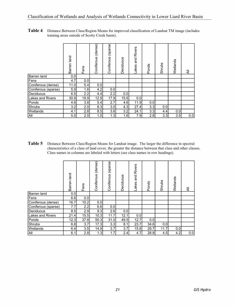
Classification of Wetlands and Analysis of Wetlands Connectivity in Lower Liard River Basin
21 GIS Hydro
Table 4 Distance Between Class/Region Means for improved classification of Landsat TM image (includes training areas outside of Scotty Creek basin).
Table 5 Distance Between Class/Region Means for Landsat image. The larger the difference in spectral characteristics of a class of land cover, the greater the distance between that class and other classes. Class names in columns are labeled with letters (see class names in row headings).
Barre
n la
nd
Fens
Con
ifero
us (d
ense
)
Con
ifero
us (s
pars
e )
Dec
iduo
us
Lake
s an
d R
iver
s
Pond
s
Shru
bs
Wet
land
s
All
Barren land 0.0Fens 4.7 0.0Coniferous (dense) 11.0 5.4 0.0Coniferous (sparse) 5.9 1.6 4.2 0.0Deciduous 6.5 2.2 4.4 2.2 0.0Lakes and Rivers 30.9 19.9 12.9 17.9 15.6 0.0Ponds 4.6 3.8 5.4 2.7 4.6 11.9 0.0Shrubs 3.2 2.0 8.3 3.0 4.3 27.4 3.3 0.0Wetlands 4.1 2.8 8.5 3.6 3.2 24.1 3.3 4.4 0.0All 5.0 2.0 1.0 1.3 1.6 7.9 2.8 3.3 3.5 0.0
Barre
n la
nd
Fens
Con
ifero
us (d
ense
)
Con
ifero
us (s
pars
e )
Dec
iduo
us
Lake
s an
d R
iver
s
Pond
s
Shru
bs
Wet
land
s
All
Barren land 0.0Fens 6.6 0.0Coniferous (dense) 16.7 10.2 0.0Coniferous (sparse) 7.7 2.2 6.6 0.0Deciduous 8.5 2.9 9.3 2.6 0.0Lakes and Rivers 21.4 15.5 10.3 11.7 12.1 0.0Ponds 12.3 37.8 50.3 31.0 49.5 12.7 0.0Shrubs 6.8 3.7 17.3 3.3 8.1 23.7 34.6 0.0Wetlands 6.4 3.5 14.9 3.7 3.7 15.8 29.7 11.7 0.0All 6.1 2.8 1.3 1.7 2.4 4.7 28.8 4.5 4.2 0.0

Classification of Wetlands and Analysis of Wetlands Connectivity in Lower Liard River Basin
22 GIS Hydro
Table 6 Area Summary Report for Landsat image classification of Lower Liard River basin.
Class/Region Hectares Sq. Km % Total Area Barren 27683.530 276.835 0.8Channel Fens 619156.680 6191.567 18.6ConFor_dense 429196.888 4291.969 12.9ConFor_sparse 979971.843 9799.718 29.5DecFor 208224.110 2082.241 6.3Lakes 798867.865 7988.679 24.0Ponds 8829.718 88.297 0.3Shrubs 116489.399 1164.894 3.5Wetlands 130829.997 1308.300 3.9All 3321998.360 33219.984 100.0
Table 7 Kappa Index of Agreement (KIA) for the same area in Scotty Creek basin for Landsat and IKONOS image classifications.
Category Landsat image IKONOS image barren 0.57 0.94ponds / shallow water 0.00 n/alakes / rivers 0.91 0.72wetlands 0.63 0.40fens 0.43 0.30shrubs 0.33 0.18deciduous forest 0.19 0.08coniferous forest (sparse) 0.29 0.34coniferous forest (dense) 0.70 0.49
overall Kappa index 0.49

Classification of Wetlands and Analysis of Wetlands Connectivity in Lower Liard River Basin
23 GIS Hydro
Appendix ІII: Data IKONOS IMAGE DESCRIPTIONSatellite
Satellite Launch Altitude Inclination Crossing Time
Ikonos 2 September 1999 681 kms 98.1° 10:30 am
Sensors
Multispectral
Bands Panchromatic 1 2 3 4
Spectral range Visible + VNIR Blue Green Red VNIR
Frequency (microns) 0.45 - 0.90 0.45 - 0.53 0.52 - 0.61 0.64 - 0.72 0.76 - 0.88
GSD (nominal at < 26° off nadir) 1 metre 4 metres
Swath Width 11 kilometres
Revisit interval 2.9 days at 1 metre resolution; 1.5 days at 1.5 metre resolution
Geometric accuracy 12-metre horizontal and 10-metre vertical accuracy with no ground control; 2-metre horizontal and 3-metre vertical accuracy with ground control
http://www.eurimage.com/Products/ikonos/tech_summ.html
IKONOS multispectral high-resolution images of Scotty Creek basin acquired summer 2000
West side of Scotty Creek basin file PO_50586.pix(52.4 MB) July 20, 2000.
East side of Scotty Creek basin file PO_50588.pix(82.2 MB) September 1, 2000.
The original resolution was 1 x 1 meter resolution for each band withcomposite (4 bands) imagery resolution of 4 x 4 meters. Raster image size of2515 columns x 4182 rows indicating the image length is greater in the North-South direction. Total ground distance covered is 10060 meters in East-Westdirection and 16728 meters in North- South direction. Total area covered16843 hectares or 168 km2.
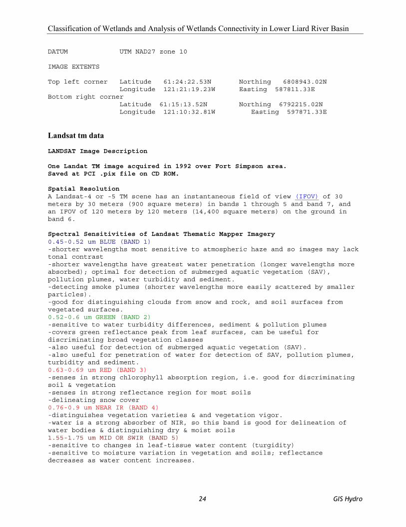
Classification of Wetlands and Analysis of Wetlands Connectivity in Lower Liard River Basin
24 GIS Hydro
DATUM UTM NAD27 zone 10
IMAGE EXTENTS
Top left corner Latitude 61:24:22.53N Northing 6808943.02NLongitude 121:21:19.23W Easting 587811.33E
Bottom right cornerLatitude 61:15:13.52N Northing 6792215.02NLongitude 121:10:32.81W Easting 597871.33E
Landsat tm data
LANDSAT Image Description
One Landat TM image acquired in 1992 over Fort Simpson area.Saved at PCI .pix file on CD ROM.
Spatial ResolutionA Landsat-4 or -5 TM scene has an instantaneous field of view (IFOV) of 30meters by 30 meters (900 square meters) in bands 1 through 5 and band 7, andan IFOV of 120 meters by 120 meters (14,400 square meters) on the ground inband 6.
Spectral Sensitivities of Landsat Thematic Mapper Imagery0.45-0.52 um BLUE (BAND 1)-shorter wavelengths most sensitive to atmospheric haze and so images may lacktonal contrast-shorter wavelengths have greatest water penetration (longer wavelengths moreabsorbed); optimal for detection of submerged aquatic vegetation (SAV),pollution plumes, water turbidity and sediment.-detecting smoke plumes (shorter wavelengths more easily scattered by smallerparticles).-good for distinguishing clouds from snow and rock, and soil surfaces fromvegetated surfaces.0.52-0.6 um GREEN (BAND 2)-sensitive to water turbidity differences, sediment & pollution plumes-covers green reflectance peak from leaf surfaces, can be useful fordiscriminating broad vegetation classes-also useful for detection of submerged aquatic vegetation (SAV).-also useful for penetration of water for detection of SAV, pollution plumes,turbidity and sediment.0.63-0.69 um RED (BAND 3)-senses in strong chlorophyll absorption region, i.e. good for discriminatingsoil & vegetation-senses in strong reflectance region for most soils-delineating snow cover0.76-0.9 um NEAR IR (BAND 4)-distinguishes vegetation varieties & and vegetation vigor.-water is a strong absorber of NIR, so this band is good for delineation ofwater bodies & distinguishing dry & moist soils1.55-1.75 um MID OR SWIR (BAND 5)-sensitive to changes in leaf-tissue water content (turgidity)-sensitive to moisture variation in vegetation and soils; reflectancedecreases as water content increases.
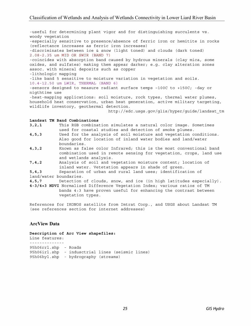
Classification of Wetlands and Analysis of Wetlands Connectivity in Lower Liard River Basin
25 GIS Hydro
-useful for determining plant vigor and for distinguishing succulents vs.woody vegetation-especially sensitive to presence/absence of ferric iron or hemitite in rocks(reflectance increases as ferric iron increases)-discriminates between ice & snow (light toned) and clouds (dark toned)2.08-2.35 um MID OR SWIR (BAND 7)-coincides with absorption band caused by hydrous minerals (clay mica, someoxides, and sulfates) making them appear darker; e.g. clay alteration zonesassoc. with mineral deposits such as copper-lithologic mapping-like band 5 sensitive to moisture variation in vegetation and soils.10.4-12.50 um LWIR, THERMAL (BAND 6)-sensors designed to measure radiant surface temps –100C to +150C; -day ornigthtime use-heat-mapping applications: soil moisture, rock types, thermal water plumes,household heat conservation, urban heat generation, active military targeting,wildlife inventory, geothermal detection.
http://edc.usgs.gov/glis/hyper/guide/landsat_tm
Landsat TM Band Combinations3,2,1 This RGB combination simulates a natural color image. Sometimes
used for coastal studies and detection of smoke plumes.4,5,3 Used for the analysis of soil moisture and vegetation conditions.
Also good for location of inland water bodies and land/waterboundaries.
4,3,2 Known as false color Infrared; this is the most conventional bandcombination used in remote sensing for vegetation, crops, land useand wetlands analysis.
7,4,2 Analysis of soil and vegetation moisture content; location ofinland water. Vetetation appears in shade of green.
5,4,3 Separation of urban and rural land uses; identification ofland/water boundaries.4,5,7 Detection of clouds, snow, and ice (in high latitudes especially).4-3/4+3 NDVI Normalized Difference Vegetation Index; various ratios of TM
bands 4:3 have proven useful for enhancing the contrast betweenvegetation types.
References for IKONOS satellite from Imtrat Corp., and USGS about Landsat TM(see references section for internet addresses)
ArcView Data
Description of Arc View shapefiles:Line features:--------------95h06rrl.shp - Roads95h06irl.shp - indusctrial lines (seismic lines)95h06hyl.shp - hydrography (streams)
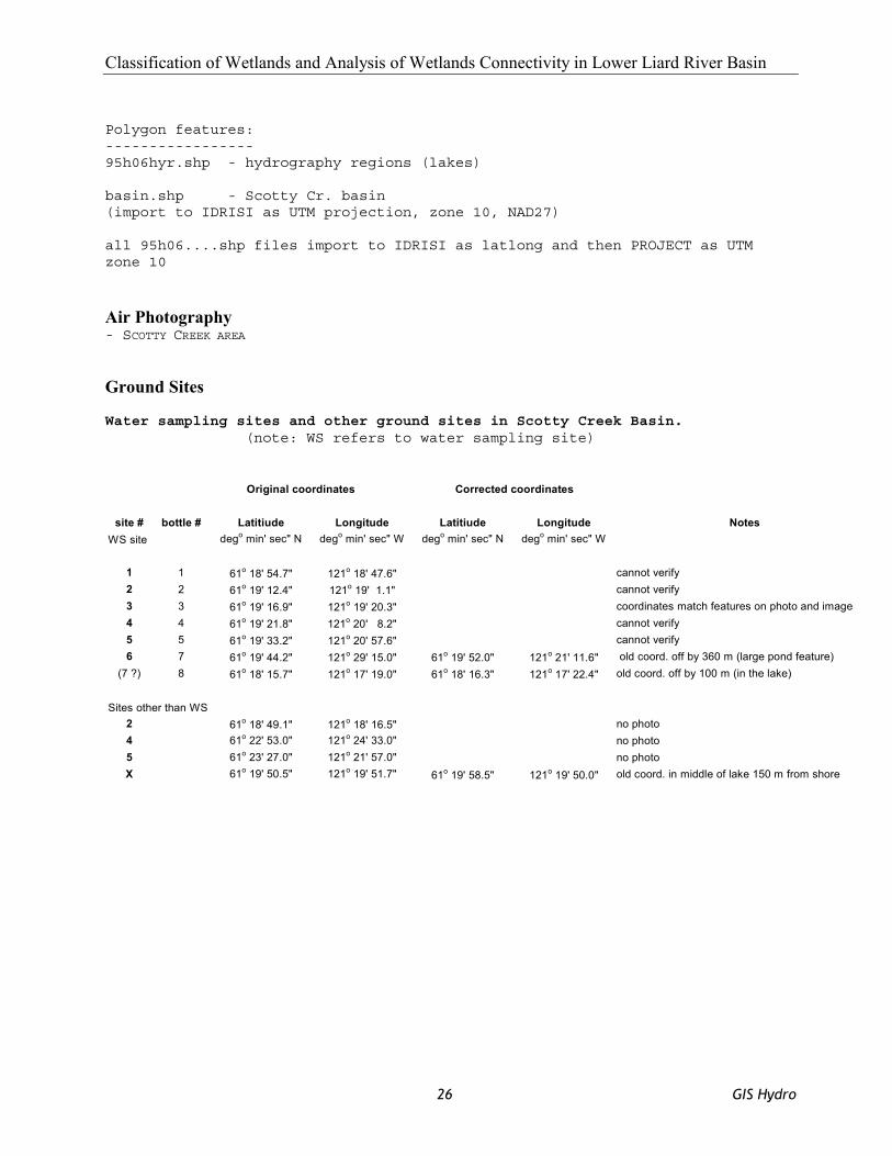
Classification of Wetlands and Analysis of Wetlands Connectivity in Lower Liard River Basin
26 GIS Hydro
Polygon features:-----------------95h06hyr.shp - hydrography regions (lakes)
basin.shp - Scotty Cr. basin(import to IDRISI as UTM projection, zone 10, NAD27)
all 95h06....shp files import to IDRISI as latlong and then PROJECT as UTMzone 10
Air Photography - SCOTTY CREEK AREA
Ground Sites
Water sampling sites and other ground sites in Scotty Creek Basin.(note: WS refers to water sampling site)
Original coordinates Corrected coordinates
site # bottle # Latitiude Longitude Latitiude Longitude NotesWS site dego min' sec" N dego min' sec" W dego min' sec" N dego min' sec" W
1 1 61o 18' 54.7" 121o 18' 47.6" cannot verify2 2 61o 19' 12.4" 121o 19' 1.1" cannot verify3 3 61o 19' 16.9" 121o 19' 20.3" coordinates match features on photo and image4 4 61o 19' 21.8" 121o 20' 8.2" cannot verify5 5 61o 19' 33.2" 121o 20' 57.6" cannot verify6 7 61o 19' 44.2" 121o 29' 15.0" 61o 19' 52.0" 121o 21' 11.6" old coord. off by 360 m (large pond feature)
(7 ?) 8 61o 18' 15.7" 121o 17' 19.0" 61o 18' 16.3" 121o 17' 22.4" old coord. off by 100 m (in the lake)
Sites other than WS2 61o 18' 49.1" 121o 18' 16.5" no photo4 61o 22' 53.0" 121o 24' 33.0" no photo5 61o 23' 27.0" 121o 21' 57.0" no photoX 61o 19' 50.5" 121o 19' 51.7" 61o 19' 58.5" 121o 19' 50.0" old coord. in middle of lake 150 m from shore

Classification of Wetlands and Analysis of Wetlands Connectivity in Lower Liard River Basin
27 GIS Hydro
Appendix ІV: Project Diagram In another PDF file.

Classification of Wetlands and Analysis of Wetlands Connectivity in Lower Liard River Basin
28 GIS Hydro
Appendix V: Pictures In another PDF file.