Graduate Theses, Dissertations, and Problem Reports

2013

Classification of Malicious Web Traffic Classification of Malicious Web Traffic

Goce Anastasovski West Virginia University

Follow this and additional works at: https://researchrepository.wvu.edu/etd

Recommended Citation Recommended Citation Anastasovski, Goce, "Classification of Malicious Web Traffic" (2013). Graduate Theses, Dissertations, and Problem Reports. 153. https://researchrepository.wvu.edu/etd/153

This Thesis is protected by copyright and/or related rights. It has been brought to you by the The Research Repository @ WVU with permission from the rights-holder(s). You are free to use this Thesis in any way that is permitted by the copyright and related rights legislation that applies to your use. For other uses you must obtain permission from the rights-holder(s) directly, unless additional rights are indicated by a Creative Commons license in the record and/ or on the work itself. This Thesis has been accepted for inclusion in WVU Graduate Theses, Dissertations, and Problem Reports collection by an authorized administrator of The Research Repository @ WVU. For more information, please contact researchrepository@mail.wvu.edu.

Classification of Malicious Web Traffic

Goce Anastasovski

Thesis submitted to theCollege of Engineering and Mineral Resources

at West Virginia Universityin partial fulfillment of the requirements

for the degree of

Master of Sciencein

Computer Science

Katerina Goseva-Popstojanova, Ph.D., ChairArun A. Ross, Ph.D.Roy S. Nutter, Ph.D.

Lane Department of Computer Science and Electrical Engineering

Morgantown, West Virginia2013

Keywords: Web 2.0 Security; Two-class classification; Multi-class classification;Semi-supervised classification; Concept drift; Feature selection

© 2013 Goce Anastasovski

Abstract

Classification of Malicious Web Traffic

Attacks targeting Web system vulnerabilities have shown an increasing trend in the recent past.A contributing factor in this trend is the deployment of Web 2.0 technologies. Due to the abilityof users to create their own content, Web 2.0 applications have become increasingly popular andin turn this has made them attractive targets for malicious attacks. Given these trends there is aneed to better understand and classify malicious cyber activities. The work presented in this thesisis based on malicious data collected by three high-interaction honeypots, and organized in HTTPsessions, each characterized by 43 different features. The data were divided into multiple vulner-ability scans and attack classes. Five batch supervised machine learning algorithms (J48, PART,Support Vector Machine SVM, Multi Layer Perceptron MLP and Naive Bayes Learner NB) andone stream semi-supervised algorithm (CSL-Stream) were used to study whether machine learningalgorithms could be used to distinguish between vulnerability scans and attacks and also amongeleven vulnerability scan and nine attack classes. The Information Gain feature selection method,and three other feature selection methods, were used to determine whether different attacks andvulnerability scans can be characterized by a small number of features (i.e., session characteris-tics). The results showed that supervised algorithms can be trained to distinguish among differentclasses of malicious traffic using only a small number of features. The stream semi-supervisedalgorithm was able to classify the partially labeled data almost as good as the completely labeleddata. The classification of the data was dependent on the number of instances in each class, dis-tinctive features for each class and amount of concept drift. The supervised algorithms, however,were better in classifying the completely labeled data.

Acknowledgments

First, I would like to thank my committee chair and adviser, Dr. Katerina Goseva-Popstojanova,for her guidance, support and encouragement throughout my graduate studies.

Also, I would like to thank Dr. Roy Nutter and Dr. Arun Ross for being my graduate committeemembers. I am grateful for the support and advice from all my graduate committee members andI am thankful for their collaboration.

This work was funded in part by the National Science Foundation under the grants CNS-0447715 and CCF-0916284.

I also want to thank and acknowledge Risto Pantev, Ana Dimitrijevik, Brandon S. Miller,Jonathan Lynch, David Krovich, and J. Alex Baker for their collaboration in the research project.

In addition, I would like to thank Dr. Hai-Long Nguyen for sharing his CSL-Stream algorithmwith me and his help.

Finally, I want to express my deepest gratitude to my mother for the support and motivationshe has given me throughout the years. I also want to thank my late father, may he rest in peace,for believing in me and always encouraging me to follow my dreams.

i

Contents

1 Introduction 1

2 Related Work 62.1 Related Work on Two-class Batch Classification . . . . . . . . . . . . . . . . . . . 62.2 Related Work on Multi-class Batch Classification . . . . . . . . . . . . . . . . . . 82.3 Related Work on Semi-supervised Classification . . . . . . . . . . . . . . . . . . . 9

2.3.1 Related Work on Batch Semi-supervised Classification . . . . . . . . . . . 92.3.2 Related Work on Stream Semi-supervised Classification . . . . . . . . . . 13

3 Data Collection, Class Labeling and Feature Extraction 153.1 Data Collection . . . . . . . . . . . . . . . . . . . . . . . . . . . . . . . . . . . . 153.2 Class Labeling . . . . . . . . . . . . . . . . . . . . . . . . . . . . . . . . . . . . 19

3.2.1 Vulnerability Scan Classes . . . . . . . . . . . . . . . . . . . . . . . . . . 193.2.2 Attack Classes . . . . . . . . . . . . . . . . . . . . . . . . . . . . . . . . 20

3.3 Feature Extraction . . . . . . . . . . . . . . . . . . . . . . . . . . . . . . . . . . . 22

4 Background on Machine Learning Algorithms and Feature Selection Methods 264.1 Batch Supervised Machine Learning Algorithms . . . . . . . . . . . . . . . . . . . 274.2 Feature Selection Algorithms . . . . . . . . . . . . . . . . . . . . . . . . . . . . . 294.3 Stream Semi-Supervised Machine Learning Algorithm . . . . . . . . . . . . . . . 30

5 Batch Supervised Two-class Classification of Malicious HTTP Traffic 325.1 Data Mining Approach for Batch Two-class Classification . . . . . . . . . . . . . 335.2 Performance Metrics For Two Class Classification . . . . . . . . . . . . . . . . . . 345.3 Results . . . . . . . . . . . . . . . . . . . . . . . . . . . . . . . . . . . . . . . . . 35

5.3.1 Can supervised machine learning methods be used to automatically distin-guish between Web attacks and vulnerability scans? . . . . . . . . . . . . . 36

5.3.2 Do attacks and vulnerability scans differ in a small number of features?Are the subsets of “best” features consistent across different data sets? . . . 38

5.3.3 Do some of the three supervised batch learning algorithms perform con-sistently better than other across multiple datasets? . . . . . . . . . . . . . 41

5.4 Using PART Rules to Characterize vulnerability scans and attacks . . . . . . . . . 43

ii

6 Batch Supervised Multi-class Classification of Malicious HTTP Traffic 456.1 Data Mining Approach for Batch Multi-class Classification . . . . . . . . . . . . . 46

6.1.1 Parameter tuning . . . . . . . . . . . . . . . . . . . . . . . . . . . . . . . 486.1.2 Performance Metrics For Multi Class Classification . . . . . . . . . . . . . 50

6.2 Results . . . . . . . . . . . . . . . . . . . . . . . . . . . . . . . . . . . . . . . . . 526.2.1 Can supervised machine learning methods be used to automatically clas-

sify different malicious classes? Are some classes harder to predict thanothers? . . . . . . . . . . . . . . . . . . . . . . . . . . . . . . . . . . . . 53

6.2.2 Do some learners perform better than others? . . . . . . . . . . . . . . . . 576.2.3 Are some features better predictors than others? . . . . . . . . . . . . . . . 626.2.4 Using PART rules to characterize different classes of malicious Web sessions 656.2.5 Addressing the class imbalance problem . . . . . . . . . . . . . . . . . . . 67

7 Stream Semi-supervised Multi-class Classification of Malicious HTTP Traffic 737.1 Data Mining Approach for Stream Semi-supervised Classification . . . . . . . . . 747.2 Based on accuracy, does J48 classify the data better than CSL-Stream? Based

on accuracy, is the classification with completely labeled data better than withpartially labeled data? . . . . . . . . . . . . . . . . . . . . . . . . . . . . . . . . . 75

7.3 Classification Based on the per Class Metrics (i.e., Fi-Score). . . . . . . . . . . . . 787.3.1 Comparison Based on Fi-Score With a Window of 1,000 Instances . . . . . 787.3.2 Comparison Based on Fi-Scores With a Window of 500 Instances . . . . . 86

7.4 Discussion . . . . . . . . . . . . . . . . . . . . . . . . . . . . . . . . . . . . . . . 91

8 Conclusion 95

Appendix A Tables for semi-supervised learning 99

iii

List of Figures

4.1 Overview of CSL-Stream (Picture adopted from [50]) . . . . . . . . . . . . . . . . 31

5.1 ROC squares for learners applied on the selected features, for WebDBAdmin I,WebDBAdmin II, Web 2.0 I, and Web 2.0 II data sets . . . . . . . . . . . . . . . . 42

6.1 Overall accuracy of the MLP with weight decay and without weight decay, usingdifferent number of units in the hidden layer. The line between the accuracy valueswas put only for visualization purposes. . . . . . . . . . . . . . . . . . . . . . . . 49

6.2 Per class recall (Ri), precision (Pi), and F-Score (Fi) for J48. The line between theF-Score values was put only for visualization purposes. . . . . . . . . . . . . . . . 53

6.3 Confusion matrices for each learner trained on all 43 features. . . . . . . . . . . . 586.4 (a) Overall accuracy for varying number of features for all learners except Naive

Bayes and (b) for all learners including Naive Bayes. The line between the overallaccuracy values was put only for visualization purposes. . . . . . . . . . . . . . . 59

6.5 Local information gain scores. . . . . . . . . . . . . . . . . . . . . . . . . . . . . 70

7.1 Accuracy of J48 and CSL-Stream when the window size was set to 1,000 instances.The line between the accuracy values was put only for visualization purposes. . . . 76

7.2 Accuracy of J48 and CSL-Stream when the window size was set to 500 instances.The line between the accuracy values was put only for visualization purposes. . . . 77

7.3 Fi-Scores averaged, for each of the 19 malicious classes, over the three pairs ofwindows with 100%, 50% and 25% labeled data. The average Fi-Scores of J48with completely labeled data are also included. In each window there were 1,000instances. The classes are ordered from left to right based on the average Fi-Scoresof J48. The line between the Fi-Scores values was put only for visualization purposes. 79

7.4 Differences in the average per class Fi-Scores, over the three pairs of windows,between 100% and 50% labeled data, 100% and 25% labeled data, and 50% and25% labeled data. . . . . . . . . . . . . . . . . . . . . . . . . . . . . . . . . . . . 80

7.5 Total number of instances in Static, Blog, Spam on Wiki, and Wiki classes . . . . . 817.6 Distribution of instances in each training and testing window by class, with 1,000

instances in each window. The y-axis presents the number of instances and thereare two ranges present, i.e., at most 50 and at most 400 instances. . . . . . . . . . . 83

iv

7.7 Fi-Scores averaged, for each of the 19 malicious classes, over the six pairs of win-dows with 100%, 50% and 25% labeled data. In each window there were 500instances. The average Fi-Scores of J48 with completely labeled data are also in-cluded. The classes are ordered from left to right based on the average Fi-Scores ofJ48. The line between the Fi-Scores values was put only for visualization purposes. 87

7.8 Distribution of instances in each training and testing window by class, with 500instances in each window. The y-axis presents the number of instances and thereare two ranges present, i.e., at most 60 and at most 200 instances. . . . . . . . . . . 89

v

List of Tables

3.1 Breakdown of malicious Web Sessions for all data sets . . . . . . . . . . . . . . . 183.2 The list of 43 features (i.e., session attributes) which were extracted from the Web

Server’s log files . . . . . . . . . . . . . . . . . . . . . . . . . . . . . . . . . . . 23

4.1 Classifiers used to distinguish among the malicious classes . . . . . . . . . . . . . 27

5.1 Summary of two-class classification results for all data sets . . . . . . . . . . . . . 375.2 Top ten features for each dataset ordered from the most to least informative . . . . 405.3 Example PART rules for vulnerability scans and attacks . . . . . . . . . . . . . . . 44

6.1 Breakdown of malicious Web Sessions across ten vulnerability scan classes andnine attack classes for multi class classification. . . . . . . . . . . . . . . . . . . . 47

6.2 Comparison of models performance in terms of the overall accuracy and time tobuild the model. . . . . . . . . . . . . . . . . . . . . . . . . . . . . . . . . . . . . 61

6.3 Ordered list of top features based on information gain, from the most to least in-formative. . . . . . . . . . . . . . . . . . . . . . . . . . . . . . . . . . . . . . . . 63

6.4 PART rules examples based on using all 43 features. . . . . . . . . . . . . . . . . 66

7.1 Mean and standard deviation of the difference in Fi-scores, averaged across thethree pairs of windows, between completely and partially labeled data. . . . . . . . 80

7.2 Increase in per class Fi-Scores averaged across all pairs of windows when the win-dow width was decreased from 1,000 to 500 instances with 100%, 50% and 25%labeled data. . . . . . . . . . . . . . . . . . . . . . . . . . . . . . . . . . . . . . . 90

7.3 Decrease in per class Fi-Scores averaged across all pairs of windows when thewindow width was decreased from 1,000 to 500 instances with 100%, 50% and25% labeled data. . . . . . . . . . . . . . . . . . . . . . . . . . . . . . . . . . . . 90

A.1 Fi-Scores values with 100%, 50% and 25% labeled data. J48 was trained and testedon 100% labeled data. In each window there were 1,000 instances. . . . . . . . . . 99

A.2 Fi-Scores values with 100%, 50% and 25% labeled data. J48 was trained and testedon 100% labeled data. In each window there were 500 instances. . . . . . . . . . . 100

vi

Chapter 1

Introduction

Just as the age of the Industrial Revolution had a profound effect on the lives of our forefathers,

today’s so-called Digital Evolution has become ubiquitous in ours. Web, computer, and mobile ap-

plications are everywhere and everything is connected to the Internet. Today it seems that without

these applications and the Internet our lives are practically unimaginable. In particular, since the

mid-1990s, the Internet has had a revolutionary impact on our culture, commerce, and the way we

live our lives. When the Internet was in its infant stage, the content on a Web site used to be the

same and unchangeable for all users. However, we have come a long way since the mid-1990’s

and so has the World Wide Web as we know it. Nowadays, with the rise of Web 2.0 technologies

the content on a Web site varies based on input parameters provided by the user or a computer, and

is different for different users.

A Web 2.0 site allows users to interact and collaborate with each other as creators of user-

generated content in a virtual community, in contrast to Web sites where people are limited to the

passive viewing of content. In addition, Web applications today are primary software solutions of

the most businesses and individuals. Web 2.0 applications, however, are abundant in software bugs.

Software bugs which lead to hacker-exploitable vulnerabilities are increasing with the amount

of functionality and complexity that the Web applications provide. Vulnerabilities in Web 2.0

1

applications result in computer security incidents which have financial and personal consequences

to both individuals and organizations.

The December, 2012 SANS report [4] considered attacks aimed at Web applications as one of

the top and most frequent attacks towards Web systems. The popularity of these applications and

their frequent exploitation motivated us to analyze attackers activities on Web systems running Web

2.0 applications. For this purpose, over a period of several years, our research group [18], [55],

[48] developed and deployed three high-interaction honeypots, each consisting of a three-tier Web

architecture (i.e. Web server, application server, and a database server). Since our honeypots had

meaningful functionality, attackers were easily attracted, which allowed us to collect four datasets

composed of only malicious HTTP traffic.

This thesis together with our previous work [18], [27], [28], [29], [30], [48], [55] is a part of

larger effort aimed at improving Web quality and Web systems security. In particular, this thesis

focuses on the classification of malicious HTTP sessions, aimed towards Web systems running

Web 2.0 applications, to several classes and also contributes toward better understanding of the

malicious traffic. By classifying and characterizing the malicious HTTP traffic we can develop

tools to better protect our systems from attackers. In this thesis, we used two types of machine

learning algorithms: supervised and semi-supervised. Supervised algorithms only work with data

which are completely labeled, while semi-supervised algorithms have the advantage of working

with data which are partially labeled. Labeling the data completely is an expensive and difficult

process. This process can be made easier if one uses partially labeled data combined with semi-

supervised learning. In this study, we further subdivide the algorithms to batch algorithms and

stream algorithms.

A batch algorithm is an algorithm that stores the whole dataset in the main memory and learns

a model from the data, either by cross validation or dividing the data into test and training datasets

[67]. In the literature, algorithms that process massive datasets whose instances come one at a time

and update their model as each instance is inspected are referred to as stream learning algorithms

2

[32], [19], [63], [50]. Unlike batch algorithms, stream algorithms do not fit all the examples in the

working memory, thus they can easily work with large volumes of data that are open ended. The

speed that is needed to classify each example and update the existing model varies from algorithm

to algorithm and in most cases is faster than batch learning algorithms.

Most of the batch learning algorithms suppose that the data generation process comes from a

stationary distribution i.e., the data generation process does not change over time. Unfortunately,

data is seldom stationary. Often, the time needed to collect the data is long. Furthermore, events

exist that can rapidly change the underlying distribution (e.g. emergence of new worms, newly

discovered vulnerabilities). Changes that occur in the underlying concept over time are called

concept drift. In addition to working with large volumes of data, stream algorithms are able to deal

with concept drift, something that cannot be handled by batch algorithms.

By using batch supervised and stream semi-supervised algorithms we were able to characterize

and successfully classify the malicious data. These algorithms gave us a closer look at the unique

traits of some classes of malicious traffic, how the malicious traffic behaves and provide basis for

developing automatic tools which can recognize and classify the malicious traffic. The results

presented in this thesis enrich the empirical evidence on malicious cyber activities and can support

areas such as generation of attack signatures and developing models for attack injection that can

be used for testing the resilience of services and systems [27], [28].

The main findings of this thesis are as follows:

• Supervised machine learning methods can be used to separate malicious HTTP traffic, with

very high probability of detection and very low probability of false alarm, into two classes

i.e. attack sessions which try to exploit an existing vulnerability in the system, and vulnera-

bility scan sessions which cause the Web server to respond with information that may reveal

vulnerabilities of the Web server and/or Web applications.

• Furthermore, supervised machine learning methods can be used to separate malicious traffic

3

to multiple classes (nine attack and eleven vulnerability scan sessions) with high recall and

precision for all but several very small classes.

• Decision tree based algorithms, J48 and PART, distinguish among malicious classes bet-

ter than Support Vector Machines (SVM), Multilayer Perceptron (MLP), and Naive Bayes

Learner (NB) and also provide better interpretability of the results.

• Several methods that address the classification problem in imbalanced datasets did not im-

prove learners performance for the very small classes with only a handfull instances.

• Malicious classes differ only in a small number of features (i.e., session characteristics).

• The supervised learning algorithm with best performance in this thesis J48, classified the

completely labeled dataset slightly better than the semi-supervised algorithm CSL-stream.

• Semi-supervised machine learning algorithms, such as CSL-Stream, can be used to classify

partially labeled data with insignificant degradation in accuracy (i.e., at most 8% on average)

compared to completely labeled data.

• The classification of the bigger classes depends on the arrival of instances (i.e., concept drift),

the number of instances per class in each window, and the distinctive features of each class.

• The semi-supervised algorithm could not detect the appearance of new classes when they

appeared, but was able to recognize them and classify them if they prevailed in future win-

dows.

The rest of this thesis is organized as follows. In Chapter 2 we present the related work on

supervised and semi-supervised classification of malicious traffic which is followed by Chapter 3

where we discuss how the data, used by the machine learning algorithms were collected, labeled

and how features were extracted. In Chapter 4 we present an overview of the supervised and

semi-supervised machine learning algorithms and features selection methods used in this thesis. In

4

Chapter 5 and Chapter 6 we present the results of the two-class and multi-class batch classification

of our data, respectively. In Chapter 7 we discuss the results of the stream semi-supervised learning

algorithm on our data. Finally, in Chapter 8 we give the concluding remarks of this thesis.

5

Chapter 2

Related Work

In this chapter, we first review the papers that use supervised two class batch classification, and

then we address the papers that do supervised multi-class batch classification. Finally, we conclude

this chapter with the related work based on semi-supervised machine learning algorithms.

2.1 Related Work on Two-class Batch Classification

Significant amount of work in the past was focused on using different machine learning methods

for intrusion detection, that is, for classification of network traffic to two classes: malicious and

non-malicious.

The work in [51] examines the state of modern intrusion detection, with an emphasis on using

data mining. The authors introduce a novel way of characterizing intrusion detection activities

called degree of attack guilt, which in essence, is a generalization of detection accuracy. That is,

detection accuracy considers whether positive or negative detections are true or false. Degrees

of attack guilt considers a continuous spectrum, rather than simply positive or negative detections.

They suggested the use of supervised machine learning algorithms in misuse detection (i.e., match-

ing known patterns of intrusion), and anomaly detection (i.e., searching for deviations from normal

6

behavior).

An intrusion detection system was used in [36] to detect attacks against Web servers running

Web based applications. The data was collected from three Web servers: (1) a production Web

server at Google, Inc., (2) a Web server from the computer science department at the University

of California, Santa Barbara and (3) a Web server from the computer science department at the

Technical University, Vienna. Several metrics were created from client requests that reference

programs at the servers and used to automatically create parameter profiles associated with Web

applications. The authors calculated several aggreagate metrics, such as Variance, Mean, and etc.,

of the created features like access times, length of the parameters, and etc. and used chi-squared

tests and Markov models to detect various attacks such as XSS, Buffer overflow, and Code Red.

One of the few publicly available datasets, which was established as a standard benchmark for

testing intrusion detection systems, is the 1998 DARPA dataset [17]. This dataset, with its several

improvements, began with research that originated from MIT Lincoln Lab [34] and later continued

in [42]. An improved versions of the 1998 DARPA dataset was developed, such as the KDD Cup

1999 dataset described in detail in [33] and the 1999 DARPA dataset [41]. The authors in [21]

applied Markov models to classify HTTP requests generated from the traffic in 1999 DARPA

dataset combined with well known vulnerabilities from the [6]. The HTTP requests strings, from

the incoming HTTP requests, were broken down into tokens and used by the Markovian models to

detect attacks against Web servers [21].

The authors in [8] analyzed the data from the Web server log files of nine different Web servers

and built an intrusion detection tool with the ability to keep track of suspicious hosts in real time.

The authors used several known Web based attacks and CGI based attacks, as well as the data

collected from the Web server log files, to create an intrusion detection tool which consisted of 8

modules. Each module was evaluated separately on a commercial Web site, however no results of

performance were presented.

7

2.2 Related Work on Multi-class Batch Classification

In this section we present an overview of the related work which used multi-class machine learning

algorithms for classification of malicious activities.

One study in [24] created a dataset consisting of 400 attack queries, aimed at Web applications,

distributed among 4 malicious classes, and 462 Web application normal (i.e., non-attack) requests

collected from the Apache log files of three servers. The attacks queries were adopted from the well

know vulnerability lists SecurityFocus [5], Unicode IIS Buqtraq [5], and Daily’s Dave vulnerability

disclosure list [1]. Because of the fine grained interpretability of results the authors used ID3

to analyze the four attacks and measured the probability of detection, false positive, and false

negatives rate of the generated trees.

In [11] two classes of normal and six classes of malicious traffic from the query stream of a

large search engine provider were investigated. To be more specific, the six classes of malicious

traffic belonged to one big group (i.e., automated or bot malicious traffic), and the two classes

of non-malicious belonged to the normal and adult users classes. The authors obtained a random

sample of approximately 100M requests from a popular search engine from a single day (August

7, 2007), of which, after data cleaning and pruning they used only 46M for analysis. In total, only

370 training and testing HTTP sessions were used for machine learning. In addition to two-class

classification (normal vs. bot traffic), the authors also performed multi-class classification. The

authors used PCA to reduce the dimensionality of the data and compared the accuracy of seven

different machine learning algorithms. They only reported accuracy which ranged from 87% to

93% in the two-class classification and 71% to 83% in the multi-class case.

A similar work in [58] suggested that malware families share typical behavioral patterns, and

thus, machine learning methods could be used to discriminate different malware behaviors. The

authors in [58] collected malware binaries via honeypots and spam-traps, and malware family

labels had been generated by running an anti-virus tool on each malware binary file. To assess be-

8

havioral patterns shared by instances of the same malware family, the behavior of each binary was

monitored in a sandbox environment and behavior-based analysis reports summarizing operations

were generated. The authors used the SVM (Support Vector Machine) algorithm to identify the

shared behavior of fourteen malware families.

In [45] the authors compared three variants of the multiclass SVM algorithms (i.e., one-versus-

one, one-versus-all, and decision tree based multiclass SVM) to the two-class SVM. These SVM

variants, as well as the two class SVM, were used for intrusion detection in the KDD Cup 1999

dataset. This dataset, in addition to the normal traffic, included four main classes of simulated at-

tacks: DoS (denial-of-service attacks such as ping-of-death, smurf, syn flood), R2L (unauthorized

access from a remote machine, for example, by guessing password), U2R (unauthorized access to

local superuser privileges by a local unprivileged user) and PROBING (surveillance and probing,

such as for example, port-scan). The authors in [45] suggested that multi-class SVM’s were not

superior to the two-class method and they also suggested that intrusion detection was inherently a

yes-or-no problem.

2.3 Related Work on Semi-supervised Classification

In this section we first review papers which have used batch semi-supervised algorithms to study

malicious traffic and intrusion detection. Then, in a similar vein, we address related work papers

that used stream semi-supervised algorithms for classification of malicious traffic.

2.3.1 Related Work on Batch Semi-supervised Classification

All papers, presented in this subsection, addressed the problem of learning when the data were only

partially labeled by using batch semi-supervised machine learning algorithms and did not consider

the presence of concept drift. The first five papers [54], [14], [37], [16], [62], discussed here,

consider the classification problem as an intrusion detection problem by distinguishing among

9

malicious and non-malicious classes. The sixth paper [59] focused on batch semi-supervised clas-

sification of malicious malware executables and benign executables.

In [54] the authors proposed an intrusion detection system using boosting algorithms for semi-

supervised learning with labeled and unlabeled data. The authors based their experiments on the

data from the KDD Cup 1999 dataset and used the labeled data for training, and the unlabeled data

for testing. For the data that have been classified well, labels were predicted and this data were

added to the labeled portion for training. With a total of 509,588 instances, of which only 6% were

labeled, the authors reported very high accuracy, probability of detection and low false alarm rate.

Another paper studied the problem of intrusion detection with two semi-supervised algorithms

(i.e., Spectral Graph Transducer and Gaussian Fields Approach) and one semi-supervised clus-

tering algorithm (MPCK-means) [14]. The two semi-supervised algorithms in this paper, were

compared to the performance of seven other traditional supervised learning methods for intrusion

detection: Nave Bayes, Bayes Network, Support Vector Machine (SVM), Random Forest, k Near-

est Neighbor (kNN), C4.5, and RBF Network. Similarly, the semi-supervised clustering algorithm

was compared to the K-means algorithm. A fraction of the KDD Cup 1999 dataset was used to

create a training and a testing dataset which had different distributions (i.e., classes that appear in

the training dataset might not appear in the testing dataset). The authors, using accuracy as an eval-

uation metric, showed that the two semi-supervised classifiers did much better than the supervised

classifiers i.e., the accuracies of Spectral Graph Transducer and Gaussian Fields Approach were

53.44% and 49.41%, respectively, and the best accuracy of the supervised learning methods was

26.13% achieved by SVM. They suggested that the reason why semi-supervised classifiers did bet-

ter than supervised classifiers was that the training data and testing data had different distributions,

or in other words the semi-supervised learner could have observed the examples in the test set and

potentially exploited the structure of their distribution. Regarding the semi-supervised clustering

algorithm a slight amount of available labeled data was enough to improve its performance and

make it to be much better than purely unsupervised learning methods. The authors, however, did

10

not mention what percentage of the data was labeled.

The authors in [37] proposed a semi-supervised approach to anomaly and misuse detection,

where a partially observable Markov decision process (POMDP) model was given as the decision

model of intrusion detection problems. This approach attempted to fuse misuse detection with

anomaly detection and to exploit the strengths of both. Their setup did not require separate training

and testing datasets i.e., the system was ran continuously, with occasional injections of newly

labeled data. When only unlabeled data was available, the system both labeled it and used it to

refine the existing model, while when labeled data became available the learner incorporated it

into the model. The data used in [37] were the data from [60] which consisted of individual time

series from 50 different UNIX users. Each users time series consisted of 15,000 UNIX commands

such as ’ls’ or ’emacs’ and was labeled as normal user or attacker. The authors varied the number

of labeled legitimate users data (0.1%, 1%, and 10%), and the amount of attacker data (1%, 10%,

50%), and reported accuracy as well as false alarm rate. They reported high accuracy (93.9%) and

low false alarm rate when the least amount of data was labeled in both classes.

A similar work [16] suggested using semi-supervised machine learning algorithms to build

an alert filter which would reduce the high false alarm rate in intrusion detection systems. The

authors used the DARPA dataset [17] for testing their approach and incorporated two metrics,

i.e., probability of detection and reduction rate, which stands for displaying the rate of the filtered

alarm. Before the dataset was used to learn a model, the authors performed feature selection using

information gain and gain ratio, and over-sampling of the positive points to reform the unbalanced

DARPA dataset. The authors constructed statistical connection features for reducing false alarm

rates, and used the Two-Teachers-One-Student (2T1S) semi-supervised learning technique [13] to

improve the performance of their approach. Also, the authors used the supervised algorithm RSVM

[40] to test their approach and compared it to 2T1S. With 10% partially labeled data, supervised

learning reduced false alerts by 64.5% and detected 74.6% true attacks. At the same time, semi-

supervised learning detected 86.1% true attacks and reduced false alerts by 81.4%. Because semi-

11

supervised algorithms exploited the information of the unlabeled data, both detection rate and

reduction rate of semi-supervised learning was significantly better than the supervised method. In

most cases, the semi-supervised learning had better results than the supervised learning.

The work in [62] used a non-parametric approach to semi-supervised learning in intrusion

detection systems. The authors trained and tested two supervised (i.e., linear Support Vector Ma-

chine (SVM) and a maximum entropy learner) and two non-parametric semi-spervised algorithms

(i.e., Laplacian Eigenmap and Laplacian Regularized Least Squares RLS) on the Kyoto2006+

dataset [61]. The Kyoto2006+ dataset is a two class problem dataset consisting of malicious and

non-malicious traffic. 10 cross-validation was used for training and testing, which means that the

temporal dependence of the data was lost, as well as, the concept drift in the data could not have

been studied. Depending on which semi-supervised algorithm was used the authors reported re-

call between 64% and 96%, and a low false positive rate (i.e., the highest reported alarm rate was

8%). The authors also examined the ability of the Laplacian RLS learner to catch unknown at-

tacks after it had been trained on normal traffic and known attacks only. In each of the 10 runs of

cross-validation a recall greater than 90% for catching unknown attacks and low number of false

positives were reported.

The authors in [59] used the Learning with Local and Global Consistency (LLGC) [70] semi-

supervised algorithm to study malware executables. In addition to that, they seeked to determine

the optimal amount of labeled data needed for good classification. They have collected a balanced

dataset which consisted of 1,000 malicious malware executables and another 1,000 normal (i.e.,

non-malicious) executables. A feature selection method, called Document Frequency (DF) was

used, to reduce the high number of features. In this work different amounts, from 10% to 90%, of

the data were labeled. Also, the authors varied the number of instances in the training set which

had labeled instances, but the number of instances in the test set, which were unlabeled, was kept

constant. The instances in the test set whose classes have been predicted, with a certain threshold of

confidence, were added to the training dataset. The process was repeated until certain conditions

12

were satisfied. The authors used several metrics to asses the results, such as recall, false alarm,

accuracy, and area under the ROC curve (AUC). The best results in terms of AUC were obtained

with a training set containing 50% of labeled instances and in terms of accuracy, the best results

were achieved with a training set containing 65% of labeled instances.

2.3.2 Related Work on Stream Semi-supervised Classification

In the previous subsection we discussed the related work which used batch semi-supervised clas-

sification of malicious traffic. Several papers which used stream semi-supervised [50], [47] and

stream unsupervised [7], [12], [15], [53] algorithms used the KDD Cup 1999 dataset to test their

novel algorithms. However, the reason why they have chosen this dataset, along with other datasets,

was because they needed large datasets (KDD Cup 1999 has close to 5 million instances) to test

their learners. Only one paper used stream semi-supervised algorithms on a dataset that was dif-

ferent than the KDD Cuo 1999 dataset. These papers mainly focus on the performance of their

learners (i.e., memory requirements, execution time, classificationquality).

In [50] the authors reported average accuracy equal to 98.06% and 85.33% with CSL-Stream

and SmSCluster learners, respectively, using a window of size 1,000 instances on the completely

labeled KDD Cup 1999 dataset. Even when the data were partially labeled (i.e., 50%, 25%, 10%)

the accuracy did not go below 95%. In this paper, per class metrics were not used, thus one cannot

tell if the learners classified the small classes well. Accuracy can be a misleading metric when the

dataset is skewed, and as a matter of fact, the KDD Cup 1999 data is skewed. In order to see how

the classification works on the small classes we used the performance metrics discussed in Chapter

6.

In [47] a window of size 2,000 instances was used on the KDD Cup 1999 dataset. The authors

in [47] were concerned with the detection of novelty (i.e., concept evolution) and used three metrics

to evaluate the learner used in [47]. The three metrics were: (1) percent of novel class instances

misclassified as existing class, (2) percent of existing class instances falsely identified as novel

13

class, and (3) Total misclassification error.

One paper [46] used stream semi-supervised algorithms on a dataset different than the KDD

Cup 1999 dataset. This paper used a stream semi-supervised algorithm, called SmSCluster, on a

botnet dataset but did not provide any details on the dataset (i.e., a reference was given to the data

in the original paper, but that reference instead of pointing to the data it pointed to the original

paper). The authors reported average accuracy in the range of 96-99% with a window size of 1,600

instances on 5% labeled data.

The authors in [53] used 32 out of the 42 features in the KDD Cup 1999 dataset to cluster the

dataset into five clusters (i.e., one normal cluster and 4 malicious clusters). The data were divided

into nine 16 MByte windows which were used for learning. The authors in [53] used SSQ (i.e.,

sum of squared distance) to evaluate the quality of the clusters. Also, memory usage and cluster

quality versus running time were analyzed.

Similarly, in [15] and [12] 32 out of the 42 features in the KDD Cup 1999 dataset were used.

Both papers used a window of 1,000 instances. In [15] grid density based approach was used to

cluster the data and SSQ was used to evaluate the quality of the clusters. The authors reported

average accuracy equal to 92.5%. In [12] purity of the clusters does not go below 90%.

In the same fashion, in [7] the average SSQ over five runs was calculated and the data were

clustered into five clusters. The size of the window was set to 2,000 instances. In addition, the

authors used micro-clusters which enabled them to build a fine grained model of the data i.e.,

neptune and smurf, which are attacks that are present in the KDD Cup 1999 dataset, were placed

into separate small clusters.

14

Chapter 3

Data Collection, Class Labeling and Feature

Extraction

In this chapter we first present how the malicious sessions had been collected and then we discuss

how the malicious sessions had been assigned to classes. We conclude this chapter by presenting

the 43 features used to characterize each session.

Collecting malicious data that is representative of current malicious activities aimed at Web

systems running Web 2.0 applications is not a trivial task and requires significant effort; therefore

the experimental setup involved several of our team members. It should be noted that the work

presented in this chapter was a part of a larger effort which was done over a period of several years

by our team members [55], [48].

3.1 Data Collection

Our team developed and deployed three high-interaction honeypots (HoneypotSystemI, Honey-

potSystemII, and HoneypotSystemIII) which ran off-the shelf operating systems and applications.

Four datasets (WebDBAdmin I, WebDBAdmin II, Web 2.0 I, and Web 2.0 II) were collected, from

15

the three honeypots. The data were organized in Web sessions, where each sessions was defined

as a sequence of requests from the same source IP address to port 80, with a time between two

successive requests not exceeding a threshold of thirty minutes [30]. Each session was labeled as

one of eleven vulnerability scan and eleven attack classes. A session was labeled as an attack if the

attacker attempted to exploit a vulnerability in at least one request in that session. This means that

some attack sessions may contain requests that scan the Web system for vulnerabilities, in addition

to request(s) that attempt to exploit vulnerabilities. If all requests in the session were used to check

for vulnerabilities then the session was labeled as vulnerability scan. We can now formally define

vulnerability scans and attacks i.e. vulnerability scans are requests that cause the Web server to re-

spond with information that may reveal vulnerabilities of the Web server and/or Web applications.

In the same context, attacks are requests intended to directly attack some part of our system.

The three honeypots and the data collection process are explained in detail in [48], [29], and

[30].

The reason why honeypots were used, was to collect only malicious traffic, without the ’noise’

of normal traffic. Collecting only malicious Web sessions was done by advertising the honeypots

using a technique called ‘transparent linking’, which involved placing hyperlinks pointing to the

honeypots on public Web pages, so that the honeypots were indexed by search engines and Web

crawlers, but could not be accessed directly by humans. Since the honeypots could not be accessed

directly by human users the only non-malicious sessions in the Web server logs consisted of sys-

tem management traffic generated by our team and legitimate Web crawlers such as Google and

MSNbot. Removing the system management traffic was a trivial task. The crawlers were removed

based on the IP addresses listed in iplists.com and other similar sites and manual inspection of the

remaining traffic.

The operating systems and applications installed on the honeypots followed typical security

guidelines and did not include user accounts with nil or weak passwords. The three honeypots had

different configurations. Also, the honeypots had been designed to resemble a real Web server,

16

that is, our team members had used three-teir network architecture consisting of a Web server,

application server, and a database. From the three honeypots, four datasets consisting of only

malicious traffic had been collected. In what follows we discuss the datasets collected, which are

presented in Table 3.1, and the configuration for each honeypot.

The first honeypot HoneypotSystemI had an Ubuntu 7.04 operating system installed on it and

collected data from June 2008 to October 2008. The three-tier architecture of this honeypot con-

sisted of an Apache2 Web server version 2.2.3-3 to process HTTP requests, PHP Server version

5.2.1, and MySQL Server version 5.0.38-0 to serve as a database.

HoneypotSystemI had a phpMyAdmin application installed on it which served as the front-end

of the MySQL server. PhpMyAdmin is one of the most popular open source tools written in PHP

designed to handle the administration of a MySQL Server over the World Wide Web.

WebDBAdmin I was the dataset collected from the HoneypotSystemI. During the five months

when HoneypotSystemI was active our team collected a total of 214 malicious sessions; 185 of

which were vulnerability scans and 29 were attacks. Class labels are explained, in details, in

subsection 3.2.

HoneypotSystemII, with Windows XP Service Pack 2 operating system installed on it, was

deployed in March 30, 2009 and collected data in two intervals (Interval 1 - from March 30 to July

26, 2009 and Interval 2 - from August 17, 2009 to January 17, 2010) in a total duration of nine

months (i.e., 273 days).

The specific three-tier architecture consisted of a Microsoft’s Internet Information Services

(IIS) Web server version 5.1 to process HTTP requests, PHP Server version 5.0.2 to serve the

PHP-based applications, and MySQL Server version 4.1 to serve as the database.

Two Web 2.0 applications had been installed on the honeypots. The first one was Wordpress

(version 2.1.1) which is a PHP-based open source blogging software widely used across the In-

ternet. The second one was MediaWiki (version 1.9.0) which is a PHP-based open source wiki

software widely used as the application base for Wikipedia.

17

Table 3.1: Breakdown of malicious Web Sessions for all data sets

WebDBAdmin I WebDBAdmin II Web 2.0 I Web 2.0 IIsessions sessions sessions sessions

Vulnerability scans: Total 185 86.45% 513 93.44% 824 73.77% 2059 43.03%DFind 17 7.94% 19 3.46% 24 2.15% 20 0.42%Other fingerprint 14 6.54% 3 0.55% 2 0.04%Static 26 12.15% 305 55.56% 181 16.20% 327 6.83%Blog 107 9.58% 690 14.42%Wiki 1 0.18% 385 34.47% 922 19.27%Blog & Wiki 73 6.54% 77 1.61%Static & Blog 10 0.90% 1 0.02%Static & Wiki 19 1.70% 3 0.06%Static & Blog & Wiki 25 2.24% 3 0.06%phpMyAdmin 77 35.98% 155 28.23% 11 0.23%Static & phpMyAdmin 51 23.83% 30 5.46% 3 0.06%

Attacks: Total 29 13.55% 36 6.56% 293 26.23% 2726 56.97%DoS 4 0.36%Password cracking phpMyAdmin user accounts 18 8.41%Password cracking Blog user accounts 9 0.81% 1 0.02%Password cracking Wiki user accounts 71 1.48%E-mail harvesting 5 2.34%Spam on Blog 23 2.06% 1411 29.49%Spam on Wiki 249 22.29% 1055 22.05%RFI 1 0.18% 4 0.36% 5 0.10%SQL injection 1 0.47% 2 0.18%XSS 2 0.18% 11 0.23%Other Attacks 5 2.34% 35 6.38% 172 3.59%

Total 214 100% 549 100% 1,117 100% 4,785 100%

During Interval 1 our team collected 1,117 malicious sessions, where 824 were recorded as

vulnerability scans and 293 as attacks. This dataset was called Web 2.0 I, and the dataset collected

during Interval 2 was called Web 2.0 II. The Web 2.0 II dataset reported 2,059 vulnerability scan

sessions and 2,726 attack sessions i.e. a total 4,785 malicious sessions.

HoneypotSystemIII had the same configuration as HoneypotSystemII’s configuration (same

operating system, Web server, application server, and database) and instead of the MediaWiki

and Wordpress applications, a phpMyAdmin application (version 2.9.1.1) had been installed. The

reason why this was done was to establish a solid base for comparison between Web systems

running Web 2.0 and Non-Web 2.0 applications regardless of the operating environment.

WebDBAdmin II was the dataset collected from the HoneypotSystemIII. This dataset had been

collected during a time period of five months (August 17, 2009 to January 17, 2010) with 513

18

vulnerability scan sessions and 36 attack sessions (in total 549 malicious sessions).

The four datasets (i.e., WebDBAdmin I, WebDBAdmin II, Web 2.0 I and Web 2.0 II) were used

in Chapter 5 where two-class classification was performed on the data. For the batch multi-class

and stream multi-class classification in Chapter 6 and Chapter 7, respectively, we merged Web 2.0

I and Web 2.0 II and into a new dataset Web 2.0 and the algorithms on it. This was possible because

Web 2.0 I and Web 2.0 II were collected from the same honeypot during different time intervals.

3.2 Class Labeling

Since our datasets consisted of only malicious traffic, each Web session was assigned into one of

eleven vulnerability scan classes or one of eleven attack classes. The breakdown of malicious Web

sessions to different vulnerability scan and attack classes for each dataset is shown in Table 3.1. In

what follows we present details of 22 vulnerability scan and attack classes.

3.2.1 Vulnerability Scan Classes

DFind is a vulnerability scanning tool used to locate an exploit that can allow the attacker to gain

root rights on the Web server by looking at the server’s configuration. DFind scans are character-

ized by ”GET/w00tw00t.at.ISC.SANS.DFind:) HTTP/1.1” HTTP request.

Other Fingerprint class consists of two other types of vulnerability scanners: Toata Scanner,

which is used to locate vulnerabilities in Web applications and Morfeus Scanner, which is used to

locate vulnerabilities in the PHP Server.

Static class includes sessions in which the attackers accessed static content (i.e., either accessed

our main index.html page and from there browsed the rest of the static pages that contained pictures

and videos, or directly accessed the pictures and video files). This category also includes the

sessions that were searching for non-existing content on the honeypot, which typically lead to

response with ”Not Found” 404 error message.

19

The Blog class and the Wiki class are two vulnerability scan classes which contain sessions

that either directly or through the homepage fingerprinted the Blog and the Wiki, respectively.

These sessions browsed the posted content, tested the functionality of the Web 2.0 applications by

following the links that had certain Blog or Wiki like functionality, tried to find RSS feeds, and so

on.

The next four classes – Blog & Wiki, Static & Blog, Static & Wiki, Static & Blog & Wiki –

represent classes which contain vulnerability scans that scanned more than one system components

in a single session.

phpMyAdmin is class label for sessions that fingerprinted the phpMyAdmin application by

sending HTTP request with one of the following four request substrings: (1) ”GET /phpmyadmin/

HTTP/1.1” requests, (2) ”/phpMyAdmin/main.php”, (3) ”/admin/phpMyAdmin/main.php”, and

(4) ”/Websql/phpMyAdmin/main.php”. From Table 3.2 we can see that phpMyAdmin is the single

most dominant malicious class on the WebDBAdmin I dataset, and the second most dominant in

WebDBAdmin II dataset.

Static & phpMyAdmin is a vulnerability scan class where the attackers accessed the static con-

tent and fingerprinted the phpMyAdmin application in the same session.

3.2.2 Attack Classes

Denial of Service (DoS) class consists of an attack which was trying to exploit the Microsoft

IIS WebDAV PROPFIND and SEARCH Method Denial of Service Vulnerability. Because this

vulnerability was fixed in Windows XP SP1 all of the requests resulted in “Not Found” 404 error

message [3] and the attacks were not successful.

Password cracking phpMyAdmin user accounts are the sessions where attackers tried to log in

the phpMyAdmin application by various username and password combinations. The majority of

the attacks in WebDBAdmin I dataset were Password cracking of phpMyAdmin user accounts, but

this was not seen in WebDBAdmin II.

20

Password Cracking Blog user accounts and Password Cracking Wiki user accounts are attack

classes in which the attackers tried to login to the administration portion of the Blog and Wiki

application, respectively. These attacks can be recognized by the use of POST HTTP Method

characterized by “action=submitlogin” portion of the request string.

E-mail Harvesting are attack sessions where attackers tried sequence of requests which in-

volved listing the directory structure, trying to access each directory available, and list the files

looking for email addresses to harvest. E-mail Harvesting was only observed on WebDBAdmin I

dataset.

Spam on Blog and Spam on Wiki are attack classes that contain sessions which posted spam on

the Blog and Wiki, respectively. Most of the posts, in addition to text, contained links toward Web

sites with spam like content.

Remote File Inclusion (RFI) attack class contains sessions which attempted to include mali-

cious code in the space provided for PHP programs. With the help of the National Vulnerabil-

ity Database (NVD) [52] we managed to identify the following specific types of RFI attacks:

CVE-2006-3771, CVE-2006-4215, CVE-2006-5402, CVE-2007-4009, CVE-2007-6488, CVE-

2008-2836, and CVE-2008-3183.

SQL injection attack class consists of security exploit in which the attacker adds Structured

Query Language (SQL) code to a Web form’s input box to gain access to resources or make changes

to data. Again, using the NVD database we identified two specific SQL injection attacks: CVE-

2007-2821 and CVE-2008-6923.

Cross-site scripting (XSS) is an attack class with sessions that inserted malicious coding into a

link that appears to be from a trustworthy source. When the user clicks on the link, the embedded

program is submitted as part of the client’s Web request and can execute on the user’s computer,

typically allowing the attacker to steal information. Our honeypot was targeted by the CVE-2007-

0308 (as labeled in the NVD database) attack.

Other Attack class consists of attacks that did not belong to any attack class described previ-

21

ously. Some specific other types of attacks included CVE-2006-6374 and CVE-2008-3906.

3.3 Feature Extraction

In order to study the malicious activities observed in our four datasets, features that characterize

malicious Web sessions had been extracted [55]. A Web session can have one or more requests, and

each session was characterized by 43 different features (i.e., session attributes) shown in Table 3.2.

Some of the features were scalars that described a specific session characteristic (e.g., Number

of request in a session, Session duration in seconds, binary indication of an ASCII control char-

acter) while other features were aggregate metrics, such as Mean, Median, Minimum, Maximum,

and Standard Deviation, of all requests within a session (e.g., Number of parameters passed in a

request substring).

In what follows, details on the 43 features used to characterize each malicious session are

provided.

The first three features, Number of requests, Bytes transferred, and Session Duration, are basic

attributes of each session and had been adopted from our previous work [29], [30].

Features 4 to 8 describe the Time between successive requests (measured in seconds) within a

single HTTP session. Since a HTTP session can have multiple requests a vector of the time be-

tween successive requests within a session was created, and the Mean, Median, Minimum, Maxi-

mum, and Standard Deviation of the time between successive requests was calculated. (If an HTTP

session contains only one request than the values of these features are zero.) These five features

are adaptation of the “avgHTMLPeriod” and “stdevHTMLPeriod” features described in [44].

Features 9 to 14 give the Number of request in a session with a particular method type (i.e.,

GET, POST, OPTIONS, HEAD, PROPFIND, and OTHER), where OTHER is the number of re-

quests that used one of the other HTTP method types: PUT, DELETE, TRACE, or CONNECT.

Similar features (i.e., “GETPerc”, “POSTPerc”, “HEADPerc”, and “OTHERPerc”) were described

22

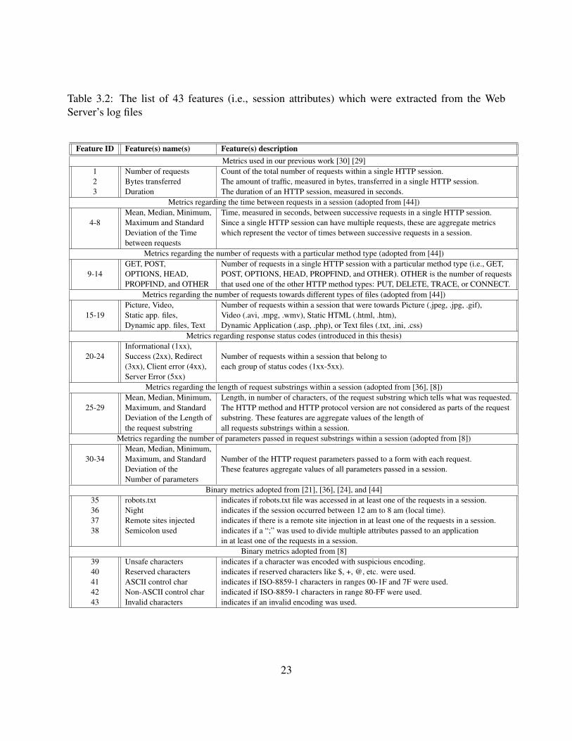
Table 3.2: The list of 43 features (i.e., session attributes) which were extracted from the WebServer’s log files

Feature ID Feature(s) name(s) Feature(s) descriptionMetrics used in our previous work [30] [29]

1 Number of requests Count of the total number of requests within a single HTTP session.2 Bytes transferred The amount of traffic, measured in bytes, transferred in a single HTTP session.3 Duration The duration of an HTTP session, measured in seconds.

Metrics regarding the time between requests in a session (adopted from [44])Mean, Median, Minimum, Time, measured in seconds, between successive requests in a single HTTP session.

4-8 Maximum and Standard Since a single HTTP session can have multiple requests, these are aggregate metricsDeviation of the Time which represent the vector of times between successive requests in a session.between requests

Metrics regarding the number of requests with a particular method type (adopted from [44])GET, POST, Number of requests in a single HTTP session with a particular method type (i.e., GET,

9-14 OPTIONS, HEAD, POST, OPTIONS, HEAD, PROPFIND, and OTHER). OTHER is the number of requestsPROPFIND, and OTHER that used one of the other HTTP method types: PUT, DELETE, TRACE, or CONNECT.

Metrics regarding the number of requests towards different types of files (adopted from [44])Picture, Video, Number of requests within a session that were towards Picture (.jpeg, .jpg, .gif),

15-19 Static app. files, Video (.avi, .mpg, .wmv), Static HTML (.html, .htm),Dynamic app. files, Text Dynamic Application (.asp, .php), or Text files (.txt, .ini, .css)

Metrics regarding response status codes (introduced in this thesis)Informational (1xx),

20-24 Success (2xx), Redirect Number of requests within a session that belong to(3xx), Client error (4xx), each group of status codes (1xx-5xx).Server Error (5xx)

Metrics regarding the length of request substrings within a session (adopted from [36], [8])Mean, Median, Minimum, Length, in number of characters, of the request substring which tells what was requested.

25-29 Maximum, and Standard The HTTP method and HTTP protocol version are not considered as parts of the requestDeviation of the Length of substring. These features are aggregate values of the length ofthe request substring all requests substrings within a session.

Metrics regarding the number of parameters passed in request substrings within a session (adopted from [8])Mean, Median, Minimum,

30-34 Maximum, and Standard Number of the HTTP request parameters passed to a form with each request.Deviation of the These features aggregate values of all parameters passed in a session.Number of parameters

Binary metrics adopted from [21], [36], [24], and [44]35 robots.txt indicates if robots.txt file was accessed in at least one of the requests in a session.36 Night indicates if the session occurred between 12 am to 8 am (local time).37 Remote sites injected indicates if there is a remote site injection in at least one of the requests in a session.38 Semicolon used indicates if a “;” was used to divide multiple attributes passed to an application

in at least one of the requests in a session.Binary metrics adopted from [8]

39 Unsafe characters indicates if a character was encoded with suspicious encoding.40 Reserved characters indicates if reserved characters like $, +, @, etc. were used.41 ASCII control char indicates if ISO-8859-1 characters in ranges 00-1F and 7F were used.42 Non-ASCII control char indicated if ISO-8859-1 characters in range 80-FF were used.43 Invalid characters indicates if an invalid encoding was used.

23

in [44] and (i.e., “method”) [8].

Features 15 to 19 represent the Number of requests within a session that were towards Picture,

Video, Static HTML files, Application specific files, and Text files, respectively. There features had

been adapted from [44].

Features 20 to 24 represent the Number of request within a session with particular response

status code. These features, were included, because the status code is an important part of the

HTTP protocol, and may provide information on attacks. For example, the status code “401 Unau-

thorized”, which indicates that the authorization has been refused for the entered credentials, may

be due to a Password cracking attack.

Features 25 to 29 represent the Mean, Median, Minimum, Maximum, and Standard Deviation

of a vector describing for each request within a session the Length of the request substring, in num-

ber of characters, which specifies what has been actually requested. For example, for the request

string “GET //phpMyAdmin//scripts/setup.php HTTP/1.1” its substring is “//phpMyAdmin//script-

s/setup.php” and its length is 31. (The substring does not include the HTTP method, in this case

“GET”, and the identification of the HTTP protocol version, in this case “HTTP/1.1”.) The Length

of the request substring feature is an adaptation of the “reqStr” feature from [8] where the ac-

tual substring was used. Similar feature, “Parameter Length”, was described in [36]. Since the

Length of substring feature is a characteristic of a single request, we calculate the Mean, Median,

Minimum, Maximum, and Standard Deviation of all substrings in a session.

Features 30 to 34 also represent a request specific feature – the Number of the parameters

passed with each request – and thus consist of Mean, Median, Minimum, Maximum, and Standard

Deviation. HTTP request parameters are the additional substrings attached to the end of a URL,

separated from the requested file with question mark “?”, when submitting a form on a Web page.

For example, the request “HTTP://www.examplesite.com/login?username=foo

&password=bar” has passed two parameters, “foo” and “bar”. This feature is similar with the

“query” feature used in [8].

24

The remaining nine features, 35 to 43, are binary variables, which were meant to capture the

existence of certain phenomena in the HTTP session. Thus, robots.txt feature indicates whether a

robots.txt file was accessed in at least one of the requests in an HTTP session, while the feature

Night indicates if the session was between 12 am to 8 am (local time). These two features were

adopted from [44]. The Remote Sites Injected feature indicates if there was a remote site injection

in at least one of the request in an HTTP session, which may help identifying XSS and RFI types

of attacks (see Subsection 3.2). The Semicolon Used feature indicates if a semicolon was used

to divide the multiple parameters passed to an application in at least one of the request in HTTP

session. Because semicolon is usually used if parameters are passed to a CGI script, the motivation

behind this feature was to capture the usage of scripts as parameters. These two features were an

adaptation of the “Value Passed” feature described in [36], [21], and [24].

The binary features 39 to 43 indicate the usage of specific characters that typically are not

associated with non-malicious request strings. These features indicate if the following was used in

at least one of the request in an HTTP session: Unsafe Characters (i.e., character with suspicious

encoding which are not in the list of safe string characters), Reserved Characters (i.e., symbols

like $, +, @, etc.), ASCII Control Characters (i.e., not printable ASCII from the ISO-8859-1

characters set in position ranges 00-1F hex (0-31 decimal) and 7F (127 decimal)), Non ASCII

Control Characters (i.e., characters that are not in the ASCII set.), consisting of the entire top

half of the ISO-8859-1 characters set, position ranges 80-FF hex (128-255 decimal), and Invalid

Characters (i.e., encoding like “%*7”.)

25

Chapter 4

Background on Machine Learning

Algorithms and Feature Selection Methods

In this chapter we present the background on the machine learning algorithms and feature selection

methods used to classify the data.

We used several batch machine learning algorithms which store the training and testing data

entirely in the working memory, i.e., the dataset is one batch, or chunk, used for training and

testing the leaning algorithms. We also used one stream algorithm which accounts for concept

drift present in the dataset, as opposed to the batch algorithms which do not have this ability.

The algorithms used in this thesis in addition to batch and stream can be classified as supervised

and semi-supervised. More specifically, the batch algorithms used in this thesis are all supervised,

and the semi-supervised algorithm used in this thesis is a stream algorithm. Supervised algorithms

only work when the data is completely labeled. On the other hand, semi-supervised algorithms can

classify partially labeled data, which is very important having in mind that the process of labeling

the data is very expensive.

In this thesis we address, both, two-class and multi-class classification problems. The batch

supervised algorithms classify the data, first into two classes (vulnerability scans and attacks), and

26

then into 19 malicious classes. We would like to note that the multiclass classification was used

only on the merged Web 2.0 I and Web 2.0 II dataset, which had 19 out of the total 22 classes (i.e.,

three classes that appeared in WebDBAdmin I and WebDBAdmin II did not appear in Web 2.o I

and Web 2.0 II). The stream semi-supervised algorithm is only used for multi-class classification.

We also use feature selection to remove ’noisy’ features, improve classification and reduce the

time needed to train the learners.

In what follows, we first provide a brief insight of how each of the batch supervised machine

learning algorithms works, and then we present the feature selection algorithms used to reduce

the number of features needed for classification. Finally, we present the stream semi-supervised

algorithm used in this thesis.

4.1 Batch Supervised Machine Learning Algorithms

In order to distinguish between vulnerability scans and attacks, as well as among the 19 classes of

vulnerability scans and attacks, we employed several batch supervised machine learning algorithms

presented in Table 4.1.

Table 4.1: Classifiers used to distinguish among the malicious classes

Classifier AbbreviationDecision tree classifier

J48 Decision Tree J48J48 Pruned Decision Tree J48 prunedPartial Decision Trees PARTPartial Decision Trees Pruned PART pruned

Support Vector Machine-based classifierSupport Vector Machine SVM

Neural Networks classifierMultilayer Perceptron MLP

Statistical classifierNaive Bayes Classifier NB

27

Decision Tree J48 is a Java implementation of the C4.5 decision tree algorithm [57], which

divides the feature space successively by choosing primarily features with the highest information

gain. Instances are classified by sorting them from the root to some leaf node, which specifies the

class of the instance. Each node of the tree specifies a test of some feature and each branch from

that node corresponds to one of the possible values for that feature. Decision trees are robust to

noisy data and capable of learning disjunctive expressions.

Partial Decision Tree PART [22] infers rules by repeatedly generating partial decision trees

by adopting the divide-and-conquer strategy of RIPPER and combining it with the decision tree

approach of C4.5. After generating each rule, the partial decision tree is discarded which avoids

early generalization.

For the tree based methods, J48 and PART, we also built the pruned trees, which optimize the

computational efficiency and classification accuracy of the tree model. When pruning methods

are applied the resulting tree is reduced in size or number of nodes in order to avoid unnecessary

complexity and over-fitting of the data. For both J48 and PART we used Reduced Error Pruning

(REP) [56].

Support Vector Machine SVM [10] implicitly maps input feature vectors to a higher dimen-

sional space by using a kernel function. In the transformed space, a maximal separating hyperplane

is built considering a two class problem. In this thesis we use a multiclass one-vs-all SVM [68]

with Radial Basis Function (RBF) as a kernel function.

An artificial neural network is a mathematical representation which was inspired by the func-

tioning of the human brain. More specifically, a neural network is a set of input units (neurones),

that are connected to other units in the hidden or output layer. Each connection has a certain weight

associated with it. In this thesis we use a Multi-Layer Perceptron MLP [49], [20] with one hidden

input layer.

Naive Bayes Learner NB [49], [20] is a statistical classifier based on the Bayes theorem. The

Bayesian approach to classifying a new instance is to assign the most probable class value, given

28

the new instance. In other words, Naive Bayes Classifier considers all features to contribute inde-

pendently to the probability that instance X belongs to class Y, whether or not they’re in fact related

to each other. An interesting approach in Naive Bayes classification is that, unlike J48, there is no

explicit search through the space of possible hypothesis, i.e., classification is done solely on the

prior probabilities, likelihood, evidence probabilities and maximum a posteriori probability of the

data and the new observed instance.

4.2 Feature Selection Algorithms

Besides applying the learners to all 43 features we also employed feature selection. The motivation

for using feature selection was to explore whether a small subset of session characteristics can be

used to efficiently distinguish among classes of malicious sessions.

There are two major approaches to feature selection: filter approach which relies only on the

data characteristics to select feature subsets and wrapper approach which involves a predetermined

machine learning algorithm as evaluation criterion. We chose a filtering approach for two reasons:

(1) it allowed us to fairly compare different machine learning methods, without tailoring the se-

lected features to specific machine learning method and (2) it was computationally more efficient.

In particular, we use information gain feature selection method which ranks the features from

the most informative to least informative using the information gain as a measure [43]. We also

tried using three other feature selection methods: (1) information gain ratio [49], (2) chi-square,

and (3) relief. However, the selected features lead to worse performance than the features se-

lected by information gain. That is why we only present the results with the features selected by

information gain.

29

4.3 Stream Semi-Supervised Machine Learning Algorithm

In many applications, totally labeled training and testing data is a rare case because labeling the

data completely generally is costly and in some occasions practically impossible.

We mentioned in the introduction of this thesis that large volumes of data streams are gener-

ated from various applications such as real-time surveillance cameras, online transactions and, of

course, network event logs. Data mining this sort of data with traditional batch learning algorithms

fails because of the large volume of the data which are coming at a very fast pace. Moreover,

because the data are arriving very fast, one is not able to label them completely. Therefore, often

we are left with partially labeled data. However, when one is faced with this sort of data all hope

for mining them and learning patterns is not lost. Semi-supervised learning algorithms have been

proposed to cope with partially labeled data.

A novel semi-supervised algorithm that deals with partially labeled data streams was pro-

posed in [50]. This stream semi-supervised algorithm was called CSL-Stream (Concurrent Semi-

supervised Learning of Data Streams). CSL-Stream is an incremental algorithm that concurrently

does clustering and classification. Figure 4.1 gives an overview of CSL-Stream’s concurrent semi-

supervised mining approach. More specifically, CSL-Stream stores a dynamic tree structure to

capture the entire multidimensional space of the data as well as a statistical synopsis of the data

stream.

Two mining tasks, clustering and classification, run at the same time and mutually improve

each other. The clustering process takes into account class labels to produce high quality clusters

and the classification process uses the clusters together with a statistical test to accurately classify

the stream. CSL-Stream also implements an incremental learning approach because the system

updates only when it becomes unstable, i.e., labeled data is classified and if low accuracy is gained

the system is updated. The system divides the data into sequential chunks and uses every odd

chunk for training and every even chunk for testing the learned model.

30

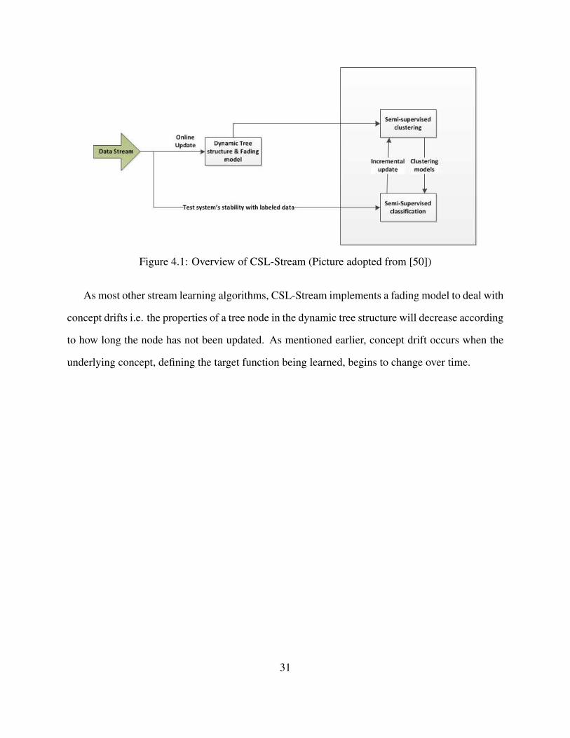
Figure 4.1: Overview of CSL-Stream (Picture adopted from [50])

As most other stream learning algorithms, CSL-Stream implements a fading model to deal with

concept drifts i.e. the properties of a tree node in the dynamic tree structure will decrease according

to how long the node has not been updated. As mentioned earlier, concept drift occurs when the

underlying concept, defining the target function being learned, begins to change over time.

31

Chapter 5

Batch Supervised Two-class Classification of

Malicious HTTP Traffic

In this chapter the problem is posed as a batch supervised two class classification problem where

we only distinguish between vulnerability scan and attack sessions using the data from the four

datasets. The results are based on the published conference paper [27] and included as a part of a

journal paper, currently under review [26].

In this chapter we address the following three research questions:

1. Can supervised machine learning methods be used to automatically distinguish between Web

attacks and vulnerability scans?

2. Do attacks and vulnerability scans differ in a small number of features? Are the subsets of

“best” features consistent across different data sets?

3. Do some of the three supervised batch learning algorithms perform consistently better than

other across multiple datasets?

32

5.1 Data Mining Approach for Batch Two-class Classification

First, as a part of data preprocessing we performed feature normalization. In our dataset, the ranges

of the features were very different. Features 1 to 34 were on an interval scale, while features 35

to 43 were binary features which took zero or one values. Normalization was applied in order to

avoid features with larger numeric ranges to dominate those with smaller numeric ranges. We used

the Min-Max Normalization in this thesis, which made each feature value to lie within the new

range [0,1].

For the two class problem we used stratified 10-fold cross-validation, on each dataset, which

involved partitioning the dataset into ten complementary subsets, and then using nine subsets as

training data and validating the results on the remaining subset (called validation data or testing

data). This process was repeated ten times, with each of the ten subsets used exactly once as

validation data.

The advantage of this method over repeated random sub-sampling is that all observations are

used for both training and validation. The results presented in this chapter of the thesis are the

averages of the ten results from the folds.

Besides applying the five supervised learners (i.e., J48, J48 Pruned, PART, PART Pruned, and

Support Vector Machine SVM) to all 43 features we also employed a feature selection method.

The motivation for using feature selection was to explore whether a small subset of session char-

acteristics could be used to efficiently separate attack sessions from vulnerability scan sessions.

In addition to learning about characteristics of malicious activities, reducing the number of fea-

tures by removing the irrelevant and noisy features speeds up the machine learning algorithms and

hopefully improves their performance [43]. As stated previously in Chapter 4, Section 4.2, in

this thesis we used the information gain feature selection method which ranks the features from

the most informative to least informative using the information gain as a measure [43]. Feature

selection was performed on the whole dataset using stratified 10 cross validation.

33

Since our goal was to identify the smallest number of features sufficient to accurately distin-

guish attacks from vulnerability scans, we used the following procedure for each individual dataset

(i.e., on Web 2.0 I, Web 2.0 II, WebDBAdmin I, WebDBAdmin II). For each learner, we started

with the highest ranked feature and included one feature at a time until reaching less than or equal

to 1% difference of the probability of detection (pd) compared to the case when all 43 features

were used. Then, we chose the smallest set of features from the best learner among all learners for

the specific dataset and used it to test the performance of all learners.

Training and testing the learners was done using WEKA [31] on a computer with 64 bit Win-

dows 7 operating system and Intel Core 2.90 GHz processor with 8 GB of RAM. The parameters

of the tree learners were set to their default values in WEKA.

5.2 Performance Metrics For Two Class Classification

To evaluate learners’ performance, we first computed the two class confusion matrix

Actual: Actual:

Vulnerability Scan Attack

Predicted:

Vulnerability Scan T N FN

Predicted:

Attack FP T P

where T N, FN, FP, and T P denote true negatives, false negatives, false positives, and true posi-

tives, respectively. Then, we computed the following metrics which assess different aspects of the

classification:

accuracy (acc) = (T N +T P)/(T N +FN +FP+T P) (5.1)

probability of detection (pd) = T P/(FN +T P) (5.2)

34

probability of false alarms (pf) = FP/(T N +FP) (5.3)

precision (prec) = T P/(T P+FP) (5.4)

balance (bal) = 1−√(0− p f )2 +(1− pd)2/

√2 (5.5)

The accuracy, given with (5.1) provides the percentage of sessions that are detected correctly.

Since attacks are more critical events than vulnerability scans probability of detection defined by

(5.2) which sometimes is also called recall, accounts for the probability of detecting an attack (i.e.,

the ratio of detected attacks to all attacks). Probability of false alarm, defined by (5.3), is the ratio

of vulnerability scans misclassified as attacks to all vulnerability scans, that is, the probability that

a vulnerability scan is falsely reported as an attack. It is important to note that our data do not have

any normal traffic (i.e., all the traffic is malicious). We would like to remind the reader that attacks

are more severe events than vulnerability scans because they try to harm targeted systems while

vulnerability scans only look for the presence of potential vulnerabilities on systems. Precision,

defined by (5.4) determines the fraction of sessions correctly classified as attacks out of all sessions

classified as attacks. Ideally, we want probability of detection to be 1 and probability of false alarm

to be 0. It appears that a rather useful metric of performance is the so called balance, which is

defined as the Euclidian distance from this ideal point of p f = 0, pd = 1 to a pair of (p f , pd). For

convenience, the balance is normalized by the maximum possible distance across the ROC square√

2 and then subtracted from 1 (see (5.5)). It follows that higher balance is better since (p f , pd)

point falls closer to the ideal point (0,1).

5.3 Results

In this section we answer the three research questions, presented in the beginning of this chapter,

using three (J48, PART, and SVM) of the supervised batch learning algorithms on the four datasets

shown in Table 3.1.

35

5.3.1 Can supervised machine learning methods be used to automatically

distinguish between Web attacks and vulnerability scans?

In order to answer this question we present Table 5.1 where the method that gives the best (worst)

probability of detection is highlighted in italic (bold). It is clear that for three out of four datasets

the learners had very high probability of detection and low probability of false alarm. More specif-

ically, the ranges for the probability of detection, when all 43 features were used, for WebDBAd-

min I, Web2.0 I, and Web2.0 II datasets were 82.76% – 96.55%, 96.92% – 98.63%, and 92.52% –

97.36%, respectively. Furthermore, the probability of false alarm in these three datasets in many

cases was less than 1% and was never above 3.69%.

As we can see in Table 5.1, WebDBAdmin II dataset had significantly lower probability of

detection (with a range of 41.67% – 75.00%) when compared to the other three datasets. Inter-

estingly, the probability of false alarm was very low for this dataset as well (less than 1.75% for

all learners). The lower probability of detection in the case of WebDBAdmin II dataset was not

unexpected, having in mind that this dataset had the smallest percentage of attacks (only 6.65%).

Even more, 35 out of total 36 observed attacks were classified as ‘Other attacks’ (see Table 3.1) be-

cause they differed among themselves. Therefore, whenever any of these attack sessions appeared

in the validation (i.e., testing) data it did not have corresponding instances in the training data. In

this context, we can say that the best performing learner J48 was able to detect 75% of the new,

previously unseen attacks. Note that in case of WebDBAdmin I dataset, even though it had only

29 attacks (i.e., 13.55% of all sessions), all learners performed significantly better than in the case

of WebDBAdmin II dataset. This is because multiple attack sessions belong to same attack classes

(see Table 3.1).

Another important observation made based on the data presented in Table 5.1 is that accuracy

on its own can be a misleading measure of learner’s performance. Specifically, when all 43 features

were used for learning the accuracy was very high (i.e., above 94%) for all datasets and all learners,

36

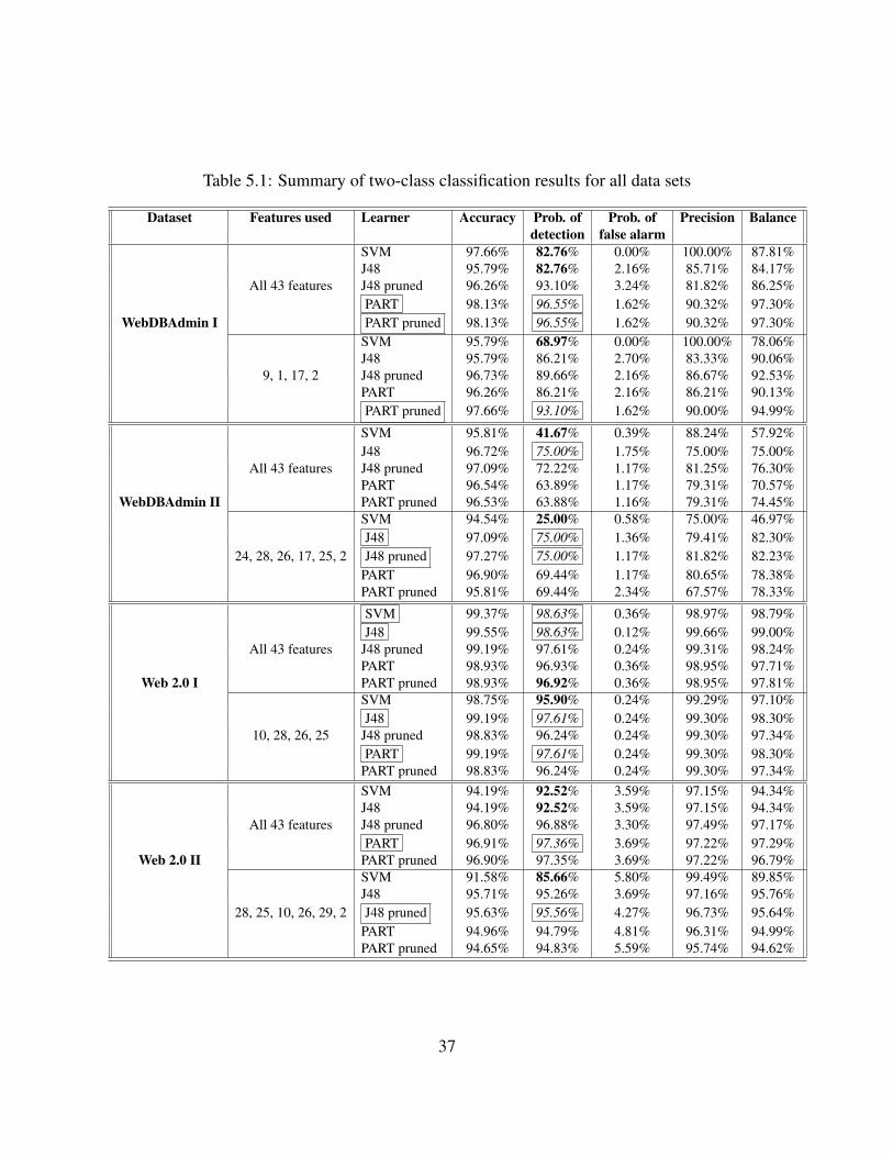
Table 5.1: Summary of two-class classification results for all data sets

Dataset Features used Learner Accuracy Prob. of Prob. of Precision Balancedetection false alarm

SVM 97.66% 82.76% 0.00% 100.00% 87.81%J48 95.79% 82.76% 2.16% 85.71% 84.17%

All 43 features J48 pruned 96.26% 93.10% 3.24% 81.82% 86.25%PART 98.13% 96.55% 1.62% 90.32% 97.30%

WebDBAdmin I PART pruned 98.13% 96.55% 1.62% 90.32% 97.30%SVM 95.79% 68.97% 0.00% 100.00% 78.06%J48 95.79% 86.21% 2.70% 83.33% 90.06%

9, 1, 17, 2 J48 pruned 96.73% 89.66% 2.16% 86.67% 92.53%PART 96.26% 86.21% 2.16% 86.21% 90.13%PART pruned 97.66% 93.10% 1.62% 90.00% 94.99%

SVM 95.81% 41.67% 0.39% 88.24% 57.92%J48 96.72% 75.00% 1.75% 75.00% 75.00%

All 43 features J48 pruned 97.09% 72.22% 1.17% 81.25% 76.30%PART 96.54% 63.89% 1.17% 79.31% 70.57%

WebDBAdmin II PART pruned 96.53% 63.88% 1.16% 79.31% 74.45%SVM 94.54% 25.00% 0.58% 75.00% 46.97%J48 97.09% 75.00% 1.36% 79.41% 82.30%

24, 28, 26, 17, 25, 2 J48 pruned 97.27% 75.00% 1.17% 81.82% 82.23%PART 96.90% 69.44% 1.17% 80.65% 78.38%PART pruned 95.81% 69.44% 2.34% 67.57% 78.33%

SVM 99.37% 98.63% 0.36% 98.97% 98.79%J48 99.55% 98.63% 0.12% 99.66% 99.00%

All 43 features J48 pruned 99.19% 97.61% 0.24% 99.31% 98.24%PART 98.93% 96.93% 0.36% 98.95% 97.71%

Web 2.0 I PART pruned 98.93% 96.92% 0.36% 98.95% 97.81%SVM 98.75% 95.90% 0.24% 99.29% 97.10%J48 99.19% 97.61% 0.24% 99.30% 98.30%

10, 28, 26, 25 J48 pruned 98.83% 96.24% 0.24% 99.30% 97.34%PART 99.19% 97.61% 0.24% 99.30% 98.30%

PART pruned 98.83% 96.24% 0.24% 99.30% 97.34%SVM 94.19% 92.52% 3.59% 97.15% 94.34%J48 94.19% 92.52% 3.59% 97.15% 94.34%

All 43 features J48 pruned 96.80% 96.88% 3.30% 97.49% 97.17%PART 96.91% 97.36% 3.69% 97.22% 97.29%

Web 2.0 II PART pruned 96.90% 97.35% 3.69% 97.22% 96.79%SVM 91.58% 85.66% 5.80% 99.49% 89.85%J48 95.71% 95.26% 3.69% 97.16% 95.76%

28, 25, 10, 26, 29, 2 J48 pruned 95.63% 95.56% 4.27% 96.73% 95.64%PART 94.96% 94.79% 4.81% 96.31% 94.99%PART pruned 94.65% 94.83% 5.59% 95.74% 94.62%

37

even in cases when the probability of detection is low to moderate (i.e., at most 75%).

Overall, as indicated by the high probability of detection in three datasets and low prob-

ability of false alarm in all four datasets, we can conclude that supervised machine learning

methods can be used to successfully distinguish between attack and vulnerability scan ses-

sions.

5.3.2 Do attacks and vulnerability scans differ in a small number of fea-

tures? Are the subsets of “best” features consistent across different

data sets?

When distinguishing between attacks and vulnerability scans it is very important to choose the sim-

plest possible model because it leads to better efficiency and performance of the machine learning

algorithms. Typically, some features have more predicting power than others and by studying these

“best” features in more details we can develop better understanding how attacks and vulnerability

scans differ. The results of using the information gain as a feature selection method and the pro-

cedure1 described in section 5.1 show that, depending on the dataset, from four to six features can

be used to classify malicious activities without significantly worsening learners performance com-

pared to when all 43 features are used. In Table 5.1 the selected features were ordered from most

to least informative. These results indicate that attacks differ from vulnerability scans only in

a small number of features (i.e., session characteristics). Specifically, out of 43 features only

10 unique features were selected across all four datasets (i.e., 1, 2, 9, 10, 17, 24, 25, 26, 28, and

29), which means that less than one quarter of the features are important for classifying malicious

traffic.

When comparing these small subsets of best predicting features across datasets, we ob-1The difference between probability of detection when using all 43 features and reduced subset of features for

WebDBAdmin I dataset could not be made less that 1% because there are only 29 attacks out of 214 sessions. 3% isthe smallest difference that could be achieved in this case. For the other three datasets the difference was set to 1%.

38

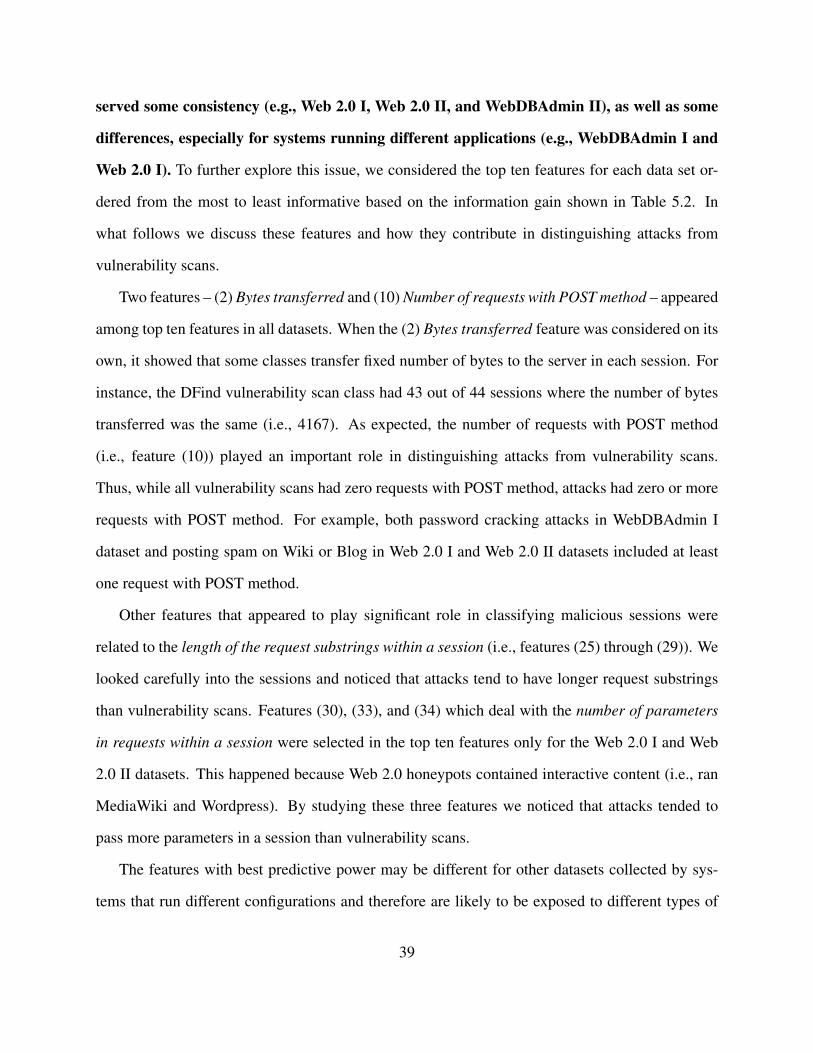
served some consistency (e.g., Web 2.0 I, Web 2.0 II, and WebDBAdmin II), as well as some

differences, especially for systems running different applications (e.g., WebDBAdmin I and

Web 2.0 I). To further explore this issue, we considered the top ten features for each data set or-

dered from the most to least informative based on the information gain shown in Table 5.2. In

what follows we discuss these features and how they contribute in distinguishing attacks from

vulnerability scans.

Two features – (2) Bytes transferred and (10) Number of requests with POST method – appeared

among top ten features in all datasets. When the (2) Bytes transferred feature was considered on its

own, it showed that some classes transfer fixed number of bytes to the server in each session. For

instance, the DFind vulnerability scan class had 43 out of 44 sessions where the number of bytes

transferred was the same (i.e., 4167). As expected, the number of requests with POST method

(i.e., feature (10)) played an important role in distinguishing attacks from vulnerability scans.

Thus, while all vulnerability scans had zero requests with POST method, attacks had zero or more

requests with POST method. For example, both password cracking attacks in WebDBAdmin I

dataset and posting spam on Wiki or Blog in Web 2.0 I and Web 2.0 II datasets included at least

one request with POST method.

Other features that appeared to play significant role in classifying malicious sessions were

related to the length of the request substrings within a session (i.e., features (25) through (29)). We

looked carefully into the sessions and noticed that attacks tend to have longer request substrings

than vulnerability scans. Features (30), (33), and (34) which deal with the number of parameters

in requests within a session were selected in the top ten features only for the Web 2.0 I and Web

2.0 II datasets. This happened because Web 2.0 honeypots contained interactive content (i.e., ran

MediaWiki and Wordpress). By studying these three features we noticed that attacks tended to

pass more parameters in a session than vulnerability scans.

The features with best predictive power may be different for other datasets collected by sys-

tems that run different configurations and therefore are likely to be exposed to different types of

39

Table 5.2: Top ten features for each dataset ordered from the most to least informative

Dataset (ID) Feature name(9) Number of requests with GET method(1) Number of requests(17) Number of requests to static files(2) Bytes transferred(21) Number of requests with ‘Success’ status code

WebDB- (3) Session duration (in seconds)Admin I (8) Std deviation of time between requests

(10) Number of requests with POST method(25) Mean length of request substrings(29) Std deviation of length of request substrings(24) Number of requests with ‘Server’ errors(28) Max length of request substrings(26) Median length request substrings(17) Number of requests to static files

WebDB- (25) Mean length of request substringsAdmin II (2) Bytes transferred

(10) Number of requests with POST method(27) Min length of request substrings(21) Number of requests with ‘Success’ status code(29) Standard deviation of length of request substrings(10) Number of requests with POST method(28) Max length of request substrings(26) Median length of request substrings(25) Mean length of request substrings

Web 2.0 I (27) Min length of request substrings(29) Standard deviation of length of request substrings(30) Mean number of parameters in requests(33) Max number of parameters in requests(2) Bytes transferred(34) Standard deviation of number of parameters in requests(28) Max length of request substring(25) Mean length of request substring(10) Number of requests with POST method(26) Median length of request substring

Web 2.0 II (29) Standard deviation of length of request substring(2) Bytes transferred(30) Mean number of parameters in requests(27) Standard deviation of length of request substring(17) Number of requests to static files(34) Standard deviation of number of parameters in requests

40

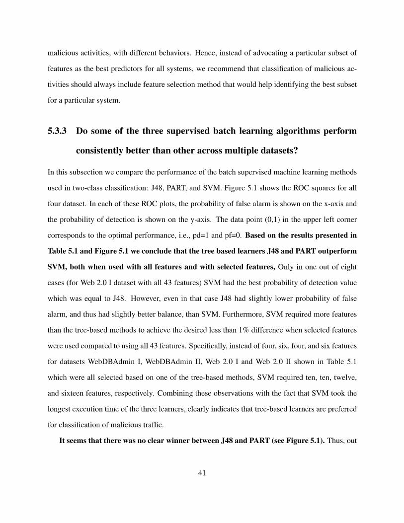
malicious activities, with different behaviors. Hence, instead of advocating a particular subset of

features as the best predictors for all systems, we recommend that classification of malicious ac-

tivities should always include feature selection method that would help identifying the best subset

for a particular system.

5.3.3 Do some of the three supervised batch learning algorithms perform

consistently better than other across multiple datasets?

In this subsection we compare the performance of the batch supervised machine learning methods

used in two-class classification: J48, PART, and SVM. Figure 5.1 shows the ROC squares for all

four dataset. In each of these ROC plots, the probability of false alarm is shown on the x-axis and

the probability of detection is shown on the y-axis. The data point (0,1) in the upper left corner

corresponds to the optimal performance, i.e., pd=1 and pf=0. Based on the results presented in

Table 5.1 and Figure 5.1 we conclude that the tree based learners J48 and PART outperform

SVM, both when used with all features and with selected features, Only in one out of eight

cases (for Web 2.0 I dataset with all 43 features) SVM had the best probability of detection value

which was equal to J48. However, even in that case J48 had slightly lower probability of false

alarm, and thus had slightly better balance, than SVM. Furthermore, SVM required more features

than the tree-based methods to achieve the desired less than 1% difference when selected features

were used compared to using all 43 features. Specifically, instead of four, six, four, and six features

for datasets WebDBAdmin I, WebDBAdmin II, Web 2.0 I and Web 2.0 II shown in Table 5.1

which were all selected based on one of the tree-based methods, SVM required ten, ten, twelve,

and sixteen features, respectively. Combining these observations with the fact that SVM took the

longest execution time of the three learners, clearly indicates that tree-based learners are preferred

for classification of malicious traffic.

It seems that there was no clear winner between J48 and PART (see Figure 5.1). Thus, out

41

0.0 0.2 0.4 0.6 0.8 1.0

0.0

0.2

0.4

0.6

0.8

1.0

probability of false alarm

prob

abili

ty o

f det

ectio

n

WebDBAdmin I

0.0 0.2 0.4 0.6 0.8 1.0

0.0

0.2

0.4

0.6

0.8

1.0

probability of false alarm

prob

abili

ty o

f det

ectio

n

WebDBAdmin II

0.0 0.2 0.4 0.6 0.8 1.0

0.0

0.2

0.4

0.6

0.8

1.0

probability of false alarm

prob

abili

ty o

f det

ectio

n

Web2.0 I

0.0 0.2 0.4 0.6 0.8 1.0

0.0

0.2

0.4

0.6

0.8

1.0

probability of false alarm

prob

abili

ty o

f det

ectio

n

Web2.0 II

Figure 5.1: ROC squares for learners applied on the selected features, for WebDBAdmin I, Web-DBAdmin II, Web 2.0 I, and Web 2.0 II data sets

of the eight cases shown in Table 5.1, J48 had the highest probability of detection in four cases,

PART in three cases, and there was one tie. The pruned versions of J48 and PART classified the

data as good as and in some occasions better that their unpruned versions.

With respect to the tree size, the number of leaves in J48 trees was comparable to the number

of rules in PART, for all datasets. Pruning the trees reduced these numbers approximately in half.

For example, unpruned J48 tree had eight leaves, while pruned J48 tree had five leaves. Similarly,

unpruned PART had eight rules and pruned PART had four rules. Interestingly, the size of the trees

and the number of rules for the Web 2.0 II dataset was significantly bigger than those generated

for the other datasets. For example, unpruned J48 tree for Web 2.0 II had 59 leaves and 117 nodes,

42

while pruned J48 tree had 33 leaves and 65 nodes. This means that Web2.0 II dataset contains

more similar instances of attacks and vulnerability scans, and therefore more complex rules were

required to divide them into two classes.

5.4 Using PART Rules to Characterize vulnerability scans and

attacks

Tree-based learners allow for high level of interpretability of the results. Table 5.3 presents sev-

eral examples of PART rules, which provide information on vulnerability scan and attack patterns

observed on our honeypots.

These rules can be used to improve the intrusion protection and detection systems, such as

firewalls and intrusion detection tools, by dynamically updating the patterns of observed attacks.

As it can be seen in Table 5.3, different rules covered significantly different numbers of instances.

For example, the first attack rule for the Web 2.0 II dataset classified correctly 2,178 out of the

2,726 attack sessions. The second attack rule, which is more complex, classified only 98 of the

2,726 attack sessions.

43

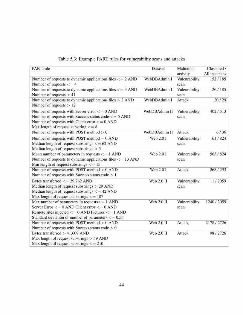
Table 5.3: Example PART rules for vulnerability scans and attacks

PART rule Dataset Malicious Classified /activity All instances

Number of requests to dynamic applications files <= 2 AND WebDBAdmin I Vulenrability 152 / 185Number of requests <= 4 scanNumber of requests to dynamic applications files <= 3 AND WebDBAdmin I Vulenrability 26 / 185Number of requests > 41 scanNumber of requests to dynamic applications files > 2 AND WebDBAdmin I Attack 20 / 29Number of requests > 12Number of requests with Server error <= 0 AND WebDBAdmin II Vulnerability 402 / 513Number of requests with Success status code <= 5 AND scanNumber of requests with Client error <= 0 ANDMax length of request substring <= 8Number of requests with POST method > 0 WebDBAdmin II Attack 6 / 36Number of requests with POST method = 0 AND Web 2.0 I Vulnerability 61 / 824Median length of request substrings <= 62 AND scanMedian length of request substrings > 5Mean number of parameters in requests <= 1 AND Web 2.0 I Vulnerability 563 / 824Number of requests to dynamic applications files <= 13 AND scanMin length of request substrings <= 15Number of requests with POST method > 0 AND Web 2.0 I Attack 268 / 293Number of requests with Success status code > 1Bytes transferred <= 29,762 AND Web 2.0 II Vulnerability 11 / 2059Median length of request substrings > 29 AND scanMedian length of request substrings <= 42 ANDMax length of request substrings <= 107Max number of parameters in requests<= 1 AND Web 2.0 II Vulnerability 1240 / 2059Server Error <= 0 AND Client error <= 0 AND scanRemote sites injected <= 0 AND Pictures <= 1 ANDStandard deviation of number of parameters <= 0.55Number of requests with POST method > 0 AND Web 2.0 II Attack 2178 / 2726Number of requests with Success status code > 0Bytes transferred > 41,609 AND Web 2.0 II Attack 98 / 2726Max length of request substrings > 59 ANDMax length of request substrings <= 210

44

Chapter 6

Batch Supervised Multi-class Classification

of Malicious HTTP Traffic

This chapter is based on the published conference paper [28] and the journal paper, currently under

review [9].

In this chapter we use only two out of the four datasets for batch supervised multi-class classi-

fication. In particular, we merged the Web 2.0 I and Web 2.0 II datasets (with 1,117 and 4,785 ma-

licious sessions, respectively) into a dataset of 5,902 sessions collected over a period of 9 months.

Merging the two datasets was possible because they were collected using the same honeypot con-

figuration (i.e., HoneypotSystemII), only at different time periods (Web 2.0 I was active from

March 30 to July 26, 2009 and Web 2.0 II from August 17, 2009 to January 17, 2010). Further-

more, two malicious classes, phpMyAdmin and Static & phpMyAdmin, were merged as one mali-

cious class called Other Vulenrability Scan. This was done because these two classes were looking

for a phpMyAdmin application which was not present on HoneypotSystemII. Consequently, the

dataset used in this chapter was composed of ten vulnerability scan and nine attack classes which

are presented in Table 6.1.

We did not use the WebDBAdmin I and WebDBAdmin II datasets for multiclass classification

45

because they were significantly smaller than Web 2.0 I and Web 2.0 II, and the number of attack

sessions was significantly smaller than vulnerability scan sessions. More specifically, the WebD-

BAdmin I dataset had 29 attack and 214 vulenrability scan sessions, whereas the WebDBAdmin II

dataset had 36 attack and 549 vulnerability scan sessions.

In this chapter we address the following three research questions:

1. Can supervised machine learning methods be used to automatically classify different mali-

cious classes? Are some classes harder to predict than others?

2. Do some learners perform better than others?

3. Are some features better predictors than others?

6.1 Data Mining Approach for Batch Multi-class Classification

In this section we present the details of our data mining approach used for the multi-class case.

Similarly, as in the two-class classification we performed feature normalization on the new

dataset, which was done on the merged Web 2.0 I and Web 2.0 II datasets.Min-Max Normalization

was applied in order to avoid features with larger numeric ranges to dominate those with smaller

numeric ranges, and this made each feature value to lie within the new range [0,1].

Then, we used stratified random sampling to select one seventh of the dataset (i.e., 844 out

of 5,902 sessions). This subset was used for tuning the parameters of the learners and for feature

selection. Feature selection on the tuning data set was performed in the following way: starting

with the highest ranked feature, selected by the information gain method, we included one feature

at a time until reaching less than or equal to 2% difference of the overall accuracy compared to the

case when all 43 features were used. The optimal parameter values were also determined on the

tuning subset.

46

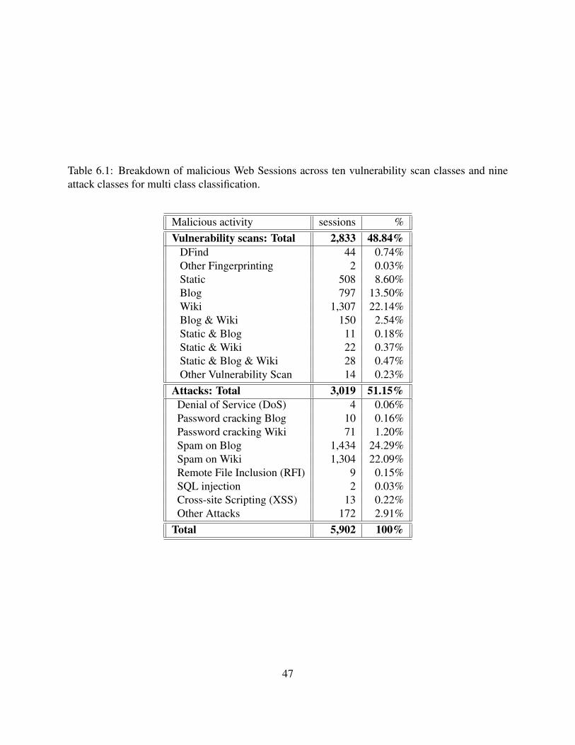
Table 6.1: Breakdown of malicious Web Sessions across ten vulnerability scan classes and nineattack classes for multi class classification.

Malicious activity sessions %Vulnerability scans: Total 2,833 48.84%

DFind 44 0.74%Other Fingerprinting 2 0.03%Static 508 8.60%Blog 797 13.50%Wiki 1,307 22.14%Blog & Wiki 150 2.54%Static & Blog 11 0.18%Static & Wiki 22 0.37%Static & Blog & Wiki 28 0.47%Other Vulnerability Scan 14 0.23%

Attacks: Total 3,019 51.15%Denial of Service (DoS) 4 0.06%Password cracking Blog 10 0.16%Password cracking Wiki 71 1.20%Spam on Blog 1,434 24.29%Spam on Wiki 1,304 22.09%Remote File Inclusion (RFI) 9 0.15%SQL injection 2 0.03%Cross-site Scripting (XSS) 13 0.22%Other Attacks 172 2.91%

Total 5,902 100%

47

On the remaining six sevenths of the data (i.e., 5,058 sessions) stratified 10 cross validation

was used to train the learners and test their classification. The reported results are averages over

the ten folds.

To distinguish among the nineteen different malicious classes we used five supervised machine

learning algorithms (i.e., J48, PART, Support Vector Machine SVM, Multi-layer Perceptron MLP,

and Naive Bayes Learner NB). As described in section 4.1, these machine learning algorithms

belong to different types of classifiers (see Table 4.1).

Similarly as in the two-class classification in Chapter 5, tuning, training and testing the learners

was done using WEKA [31] and LIBSVM [2] on a computer with 64 bit Windows 7 operating

system and Intel Core 2.90 GHz processor with 8 GB of RAM.

6.1.1 Parameter tuning

Four of the five classification algorithms had adjustable parameters, which enable an adaptation

of the algorithm to a specific problem. It is known that a careful tuning of such parameters is

essential to obtaining a representative assessment of the classifiers potential [2]. Therefore, we

carefully tuned the model’s parameters using the tuning subset consisting of one seventh of the

data.

The biggest influence on the size and accuracy of the decision tree has the parameter which is

concerned with the minimum number of instances in leaf and the confidence factor used in post

pruning. We used stratified 10 cross validation grid search on the tuning subset (i.e., one seventh

of the dataset) and determined that a value of 1 for the minimum number of instances in leaf

parameter gives best results for both J48 and PART. The confidence factor for J48 and PART were

0.1842 and 0.1211, respectively.

The classification accuracy of SVM when RBF kernel is used is highly dependent on two pa-

rameters: the gamma and cost value [2]. We used a grid-search with stratified 10 cross validation

on the tuning subset to select the best pair of gamma and cost values which maximize the classifi-

48

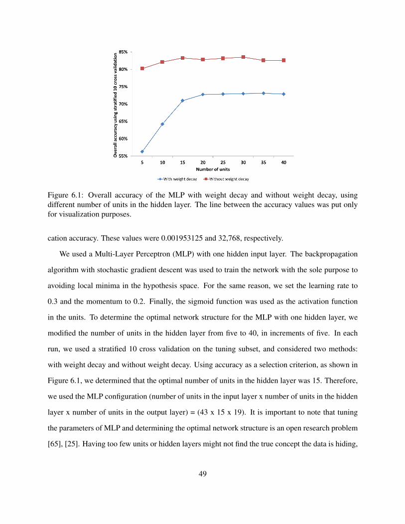
Figure 6.1: Overall accuracy of the MLP with weight decay and without weight decay, usingdifferent number of units in the hidden layer. The line between the accuracy values was put onlyfor visualization purposes.

cation accuracy. These values were 0.001953125 and 32,768, respectively.

We used a Multi-Layer Perceptron (MLP) with one hidden input layer. The backpropagation

algorithm with stochastic gradient descent was used to train the network with the sole purpose to

avoiding local minima in the hypothesis space. For the same reason, we set the learning rate to

0.3 and the momentum to 0.2. Finally, the sigmoid function was used as the activation function

in the units. To determine the optimal network structure for the MLP with one hidden layer, we

modified the number of units in the hidden layer from five to 40, in increments of five. In each

run, we used a stratified 10 cross validation on the tuning subset, and considered two methods:

with weight decay and without weight decay. Using accuracy as a selection criterion, as shown in

Figure 6.1, we determined that the optimal number of units in the hidden layer was 15. Therefore,

we used the MLP configuration (number of units in the input layer x number of units in the hidden

layer x number of units in the output layer) = (43 x 15 x 19). It is important to note that tuning

the parameters of MLP and determining the optimal network structure is an open research problem

[65], [25]. Having too few units or hidden layers might not find the true concept the data is hiding,

49

whereas having too many units or hidden layers will learn an overly complex, time consuming and

inefficient model of the true hidden concept.

6.1.2 Performance Metrics For Multi Class Classification

To evaluate the performance of each learner, we computed the confusion matrix given with equa-

tion (6.1). For each class i out of total m classes, the diagonal element Eii is equal to the number of

sessions that actually belong to i-th class and are correctly assigned to this class, which is referred

to as true positives T Pi. Each off-diagonal element Ei j, i 6= j gives the number of sessions that

actually belong to the i-th class that have been incorrectly assigned to class j.

E11 E12 . . . E1 j . . . E1m

E21 E22 . . . E2 j . . . E2m

. . . . . . . . . . . . . . . . . .

Ei1 Ei2 . . . Ei j . . . Eim

. . . . . . . . . . . . . . . . . .

Em1 Em2 . . . Em j . . . Emm

(6.1)

Then, we use the confusion matrix to compute metrics for each class individually and for all

classes together.

Per class metrics. For each individual class i, let TPi denote true positives (the number of

the sessions that in fact belong to i-the class and are correctly assigned to this class); FPi denote

false positives (the number of the sessions that in fact do not belong to i-th class, but are falsely

assigned to this class); FNi denote false negatives (the number of the sessions that in fact belong

to i-th class, but are falsely not assigned to this class); and TNi denote true negatives (the number

of the sessions that in fact do not belong to i-th class and are correctly not assigned to this class).

50

For each class i we compute the recall (Ri) and precision (Pi) as follows:

Ri = TPi/(TPi +FNi) (6.2)

Pi = TPi/(TPi +FPi) (6.3)

Recall (Ri) defined by (6.2), which sometimes is also called probability of detection, accounts

for the probability of correctly classifying the sessions of each class (i.e., the ratio of detected

sessions of class i to all sessions in class i). Precision (Pi), defined by (6.3), determines the fraction

of sessions correctly classified to belong to class i out of all sessions classified as class i. The

F-score (Fi) of each class i is then computed as a harmonic mean of the Ri and Pi as:

Fi = 2RiPi/(Ri +Pi) (6.4)

Harmonic mean is a mean metric of choice when dealing with rates or ratios, as in the case of

recall and precision. It has several desirable properties, such as it is not very sensitive to outliers

and min(Ri,Pi) ≤ Fi ≤ max(Ri,Pi). Also, the harmonic mean is smaller than both the geometric

and arithmetic mean. Ri, Pi, and Fi values are in the interval [0,1]; larger values correspond to

better classification. Ideally, we want both recall and precision to be 1, which leads to F-score

equal to 1. If either one is 0, F-score is 0 by definition.

Metrics for all classes. To evaluate the learners’ performance for all m classes together, that

is, for the entire classification problem, we use the overall accuracy given by

accuracy = TP/(TP+FN) =m

∑i=1

TPi/m

∑i=1

(TPi +FNi) (6.5)

The overall accuracy gives equal weight to each malicious session, regardless of the class distribu-

tion, and therefore it tends to be dominated by the classifier’s performance on common (i.e., high

51

frequency) classes.

In order to account for the classes and the distribution of malicious sessions among classes,

we introduce a weighted averaging approach, which takes into account the frequency of each class

in computing the average metrics for all classes. The weighted recall and precision reduce to

arithmetic average metrics if all classes are given the same weight. Arithmetic averages typically

are not used in multiclass classification because they are heavily influenced by the low frequency

classes, and thus provide very pessimistic estimates. Let mi denote the number of instances in the

i-th class. Then the weight of the i-th class is the fraction of sessions that belong to class i and it is

given by wi = mi/∑mi=1 mi. The weighted-recall is then defined as

weighted-R =m

∑i=1

(wiRi) (6.6)

The weighted precision is defined similarly and the weighted-F score is computed as a harmonic

mean of the weighted-R and weighted-P.

6.2 Results

Similarly as in the two-class problem, in this section we answer the three research questions pre-

sented in the introduction of this chapter, using all five supervised batch learning algorithms (i.e.,

J48, PART, SVM, MLP and NB). For the tree based learners we also used their pruned versions

(i.e., J48 Pruned and PART Pruned)

52

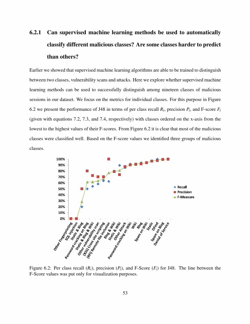
6.2.1 Can supervised machine learning methods be used to automatically

classify different malicious classes? Are some classes harder to predict

than others?

Earlier we showed that supervised machine learning algorithms are able to be trained to distinguish

between two classes, vulnerability scans and attacks. Here we explore whether supervised machine

learning methods can be used to successfully distinguish among nineteen classes of malicious

sessions in our dataset. We focus on the metrics for individual classes. For this purpose in Figure

6.2 we present the performance of J48 in terms of per class recall Ri, precision Pi, and F-score Fi

(given with equations 7.2, 7.3, and 7.4, respectively) with classes ordered on the x-axis from the

lowest to the highest values of their F-scores. From Figure 6.2 it is clear that most of the malicious

classes were classified well. Based on the F-score values we identified three groups of malicious

classes.

Figure 6.2: Per class recall (Ri), precision (Pi), and F-Score (Fi) for J48. The line between theF-Score values was put only for visualization purposes.

53

The first group consisted of ten classes, each with F-score above 80%. These ten classes

together accounted for 95.94% of all malicious sessions in our dataset. Out of these ten classes

eight had F-score above 90%. The five largest classes (i.e., vulnerability scans classes Static, Blog,

Wiki and attack classes Spam on Blog and Spam on Wiki) all belonged to this group of the best

classified classes. Interestingly, three very small classes – DoS, DFind, and Password cracking on

Wiki, with 0.08%, 0.73% and 1.19% of malicious sessions, respectively – were also in the best

classified group with all three metrics above 90%. Among the ten classes with F-score above 80%

were two other small classes Static & Wiki and Other Attacks, each with less than 3% of malicious

sessions.

The second group consisted of six classes which had F-scores in the range from 60 – 80%.

These six classes were also classified with very high recall and precision values, even though

together they accounted for only 3.79% of the total malicious sessions in our dataset. The largest

class in this group was the vulnerability scan class Blog & Wiki, which had 129 instances (i.e.

2.55% of malicious sessions) and F-score of 79.5%. The remaining five classes in this group (i.e.,

the attack classes RFI, XSS, and Password cracking on Blog, and vulnerability scan classes Other

vulnerability scan, and Static & Blog & Wiki) each had less than 0.5% of all sessions.

The last, third group of classes consisted of only three classes which had F-scores below 30%

and together accounted for only 0.26% of the malicious sessions. Two of these three classes SQL

injection and Other Fingerprinting were not classified correctly at all, which was not surprising

having in mind that they consisted of only one and two sessions, respectively. The vulnerability

class Static & Blog (which had Recall, Precision and F-score values of 20%, 50% and 28.6%,

respectively) was also very small and had only 10 sessions.

Similarly as in the two-class problem, J48 efficiently distinguished among multiple vul-

nerability scan and attack classes, with high recall and precision values for all but several

very small classes. Specifically, 16 out of 19 classes had F-score over 60%, including eight

classes which had F-score over 90%. In addition to the five largest classes, several very small

54

classes were also among the best classified.

Our results also showed that some classes were harder to classify than others. For instance,

the SQL Injection attacks, and the vulnerability scans Other fingerprinting and Static & Blog were

not classified well. Conversely, other comparably small classes were much better classified, such

as for example (RFI) Remote file inclusion with F-score around 77% or DoS with a perfect F-score

of 100%.

The classification results for the small classes in related work were substantially worse. Specif-

ically, in [69] the recall values of 21.4% and 11.2% were reported for two small classes consisting

of 0.5% and 5.9% of the whole dataset, respectively. Similarly, in [39] two small classes with

comparable sizes were reported to have recall values of 75% and 60%, respectively. Many small

classes in our dataset were classified well, such as for example DoS and DFind, which consisted of

only 0.06% and 0.74% of the whole dataset but had recall of 100%, followed by Static, Password

cracking Wiki, and Static & Wiki (with sizes of 8.6%, 1.2%, and 0.37%, respectively), which had

recall values of 97%, 91.7%, and 89.5%, respectively.

In a multiclass setting there are two reasons why some classes have significantly lower recall

and/or precision values than others. The obvious reason for poor classification is the lack of suf-

ficient number of positive training examples. In some domains this problem may be resolved by

obtaining more training cases for such classes. However, we believe this is not always possible

in case of malicious activities. For instance, even though we collected data over nine months pe-

riod, we observed only a few SQL Injection and Other Fingerprinting sessions out of total 5,902

malicious Web sessions.

In addition, some small classes were classified worse than others because they might have

less predictive features. For example, in the case of J48, the Cross-site scripting (XSS) class with

eleven sessions had recall of 63.36% and precision of 70%. On the other side, the DoS class, which

consisted of only four sessions, was detected with 100% recall and precision. Several aspects of

machine learning for imbalanced datasets such as ours are further discussed in Section 6.2.5.

55

We also looked at some of the instances which were misclassified. For example, the instances

in the Static & Blog class were most often classified as the instances in the Blog class. The reason

why this happened is due to the fact that these two classes are somewhat similar, i.e., the Static &

Blog class covered the HTTP sessions that fingerprinted both the Blog and static content on our

honeypot, where as the Blog class covered the HTTP sessions that fingerprinted only the Blog.

Similarly, the instances in the Static & Blog & Wiki classes were most often classified either as

the instances of the Static & Blog or the Static & Wiki class. Also, the instances in the Other

Vulnerability Scan class were most often classified as the instances of the Static class because

the instances of the Other Vulnerability Scan class were sessions which fingerprinted the static

content on our honeypot and looked for a phpMyAdmin application which was not installed on our

honeypot. Regarding the attack classes, we observed that the instances in the Password cracking

on Blog class were very often misplaced as the instances of the Spam on Blog class. The instances

from the Password cracking on Blog class were misclassified as the Spam on Blog because both

attacks require the attacker to use the POST method with a certain number of parameters on the

Blog application. In addition, the number of training instances of the Password cracking on Blog

class were not enough for the learner to learn the characteristics of this class and distinguish it

from the Spam on Blog. It appears that the small classes that had similar characteristics to the big

classes were often misclassified as one of the big classes.

In summary, we conclude that malicious Web activities can be successfully classified, us-

ing supervised machine learning methods, both in terms of classes and total number of in-

stances. In the case of J48, the top eight best classified classes had recall, precision, and F-score

above 90%. These eight classes contained more than 92% of all instances, and in addition to

the five largest classes included several very small classes. Only three very small classes, which

together account for 0.26% of all malicious sessions, were not classified well (i.e., have recall,

precision, and F-score less than 30%).

Detailed results for the remaining four learners are omitted due to space limitations. In the

56

following section we present the comparative analysis of learners’ performance.

6.2.2 Do some learners perform better than others?

In this section we compare the learners with respect to classification of individual malicious classes

(using the heat map representation of the corresponding confusion matrices), overall accuracy,

number of selected features, and the time to build the model.

The confusion matrices of malicious classes for all learners (including the pruned versions of

J48 and PART) are represented by the heat maps shown in Figures 6.3 (a) – (g). In these figures

the density of each cell, which is represented by shades of grey, gives the percentage of a true

malicious class assigned to a predicted class by the classifier. The main diagonal corresponds to

correct classification assignments. For a good classifier, the cells on the main diagonal are darkest

among all cells and there are not many non-zero (i.e., not white) off-diagonal cells.

The tree-based learners J48 and PART (shown in Figures 6.3 (a) and (b), respectively) out-

performed the other learners, with their corresponding pruned versions (see Figures 6.3 (d) and

(e)) having slightly worse results. SVM and MLP (shown in Figures 6.3 (c) and (f), respectively)

did worse than tree-based learners J48 and PART. Finally, Naive Bayes classifier was the worst

among classifiers used in this thesis, which is obvious from the shades of gray scattered all over its

confusion matrix shown in Figure 6.3 (g).

The reason Naive Bayes classifier did much worse than the other learners is the fact that it is

based on a simplifying assumption that the feature values are conditionally independent given the

class value [49], which is not the case with our data. In some cases, NB algorithm may generalize

well on unseen testing data even thought the independence assumption has not been satisfied, but

unfortunately this was not the case with our data.

Next, we compare the learners performance with respect to the overall accuracy, for different

number of features. As discussed in Section 6.1, we used the information gain method for feature

selection.

57

abcdefghijkl

mnopqrs

a b c d e f g h i j k l m n o p q r sPredicted Malicious Class

Act

ual M

alic

ious

Cla

ss

Scale0.000.250.500.751.00

abcdefghijkl

mnopqrs

a b c d e f g h i j k l m n o p q r sPredicted Malicious Class

Act

ual M

alic

ious

Cla

ss

Scale0.000.250.500.751.00

abcefghijkl

mnopqrst

a b c d e f g h i j k l m n o p q r s tPredicted Malicious Class

Act

ual M

alic

ious

Cla

ss

Scale0.00.20.40.60.81.0

(a) J48 (b) PART (c) SVM

abcdefghijkl

mnopqrs

a b c d e f g h i j k l m n o p q r sPredicted Malicious Class

Act

ual M

alic

ious

Cla

ss

Scale0.000.250.500.751.00

abcdefghijkl

mnopqrs

a b c d e f g h i j k l m n o p q r sPredicted Malicious Class

Act

ual M

alic

ious

Cla

ss

Scale0.000.250.500.751.00

abcdefghijkl

mnopqrs

a b c d e f g h i j k l m n o p q r sPredicted Malicious Class

Act

ual M

alic

ious

Cla

ss

Scale0.000.250.500.751.00

(d) J48 pruned (e) PART pruned (f) MLP

abcdefghijkl

mnopqrs

a b c d e f g h i j k l m n o p q r sPredicted Malicious Class

Act

ual M

alic

ious

Cla

ss

Scale0.000.250.500.751.00

a = SQL injection l = Staticb = Denial of Service m = Other attackc = Spam on Wiki n = Password cracking on Wikid = Spam on Blog o = Spam on Wikie = Password cracking on Blog p = Wikif = Other vulnerability scan q = Blog & Wikig = DFind r = Blogh = Other fingerprinting s = Spam on Blogi = (XSS) Cross site scriptingj = (RFI) Remote file inclusionk = Static & Blog &

Wiki(g) NB

Figure 6.3: Confusion matrices for each learner trained on all 43 features.

58

Figure 6.4 shows how the overall accuracy was affected by changing the number of features,

selected by information gain, from five to 43, in increments of five. Note that the features in

Figure 6.4 were included using the ranked list by the information gain, starting from the most

informative to least informative.

(a) (b)

Figure 6.4: (a) Overall accuracy for varying number of features for all learners except Naive Bayesand (b) for all learners including Naive Bayes. The line between the overall accuracy values wasput only for visualization purposes.

We first discuss the results shown in Figure 6.4 (a), which shows all learners except Naive

Bayes. As it can be noticed, J48 and PART outperformed the other learners, with no significant

difference between them and overall accuracy between 91% and 94%. The pruned J48 and PART

did worse than unpruned J48 and PART by only 0.34% to 1.38%, depending on the number of

features used. The same observation can be made comparing Figures 6.3 (a) and (d) for J48

unpruned and J48 pruned, and Figures 6.3 (b) and (e) for PART unpruned and PART pruned. That

is, the pruned versions of the learners had slightly darker shades in some off-diagonal cells of the

confusion matrix when compared to the unpruned versions.

Furthermore, both pruned and unpruned versions of J48 and PART outperformed SVM and

MLP, with a bigger difference for smaller number of features. The overall accuracy for SVM and

MLP ranged between 72%-88% and 79%-87%, respectively.

59

The overall accuracy of the Naive Bayes classifier, as it can be seen from Figure 6.4 (b), was

the worst of all learners. Even more, it showed different trend as we varied the number of features

in the order provided by information gain. Specifically, the Naive Bayes classifier had the highest

overall accuracy of 68.20 % when the top five features were used, which then decreased with

increasing the number of features. The overall accuracy of this learner dropped when more features

were added because of its statistical nature, i.e., because classification relies on the distributions

of the training data. In particular, our dataset is imbalanced and the largest classes (i.e., Spam

on Blog and Spam on Wiki) dictated what features were selected as the top five. The distribution

of the training data, when these five features were considered, tended to be similar to the unseen

testing data. Therefore, adding more features in the case of NB added noise, which resulted in

poor classification on previously unseen data and thus deteriorated the overall accuracy. This was

not the case with the rest of the learners because their classification mechanism did not rely solely

on the distribution of the data; rather, classification was done by performing a search through the

space of all possible hypotheses and adopting the hypothesis that best classified the training data.

The highest values of the overall accuracy reported in the related work were 69% in [35] and

83% in [11]. These values were significantly lower than the overall accuracy of our best learners

J48 and PART, which is in the range from 91% to 94%.

One of our goals was for each learner to find the simplest possible model that can accurately

distinguish among different malicious classes. For all learners, except NB, we used a similar

approach, as is noted in the beginning of this chapter (section 6.1), to find the simplest model.

Starting with the highest ranked feature, selected by the information gain method, we included one

feature at a time until reaching less than or equal to 2% difference of the overall accuracy compared

to the case when all 43 features were used.

The overall accuracy with all and selected features for all learners, as well the time it took to

build the models are given in Table 6.2. (We also computed the values of the weighted recall using

equation (6.6), which differed less than 1% from the corresponding values of the overall accuracy,

60

Table 6.2: Comparison of models performance in terms of the overall accuracy and time to buildthe model.

Feature Learner Overall Time to buildrank accuracy the model1 - 43 J48 93.77% 0.40 sec1 - 43 J48 Pruned 93.43% 0.19 sec

All 1 - 43 PART 94.14% 1.91 secfeatures 1 - 43 PART Pruned 93.11% 0.66 sec

1 - 43 SVM 87.80% 3.59 sec1 - 43 MLP 86.79% 65.23 sec1 - 43 NB 41.45% 0.04 sec1 - 6 J48 91.93% 0.08 sec

Information 1 - 7 J48 Pruned 91.61% 0.08 secGain 1 - 8 PART 92.60% 0.49 secselected 1 - 6 PART Pruned 91.16% 0.16 secfeatures 1 - 24 SVM 86.35% 2.38 sec

1 - 19 MLP 85.17% 49.56 sec1 - 5 NB 68.20% 0.05 sec

and therefore are not reported in Table 6.2. This phenomenon is due to the fact that classes with

low recall were extremely small (i.e., less than 1%) and thus had very small effect on the weighted

recall.)

As it can be seen in Table 6.2, SVM and MLP needed more features than J48 and PART to

achieve accuracy within 2% of the case when all features were used. Specifically, SVM and MLP

needed 24 and 19 features, respectively, i.e., three to four times as many features as J48 and PART

to achieve accuracy within 2% of the case when all features were used. When the top six features

were used to build the models of all learners, SVM and MLP had much lower accuracy (i.e., 73%

and 79%, respectively) than J48 and PART (i.e., 92%).

As shown in Table 6.2, the pruned versions of J48 and PART produced the classification results

much faster than the unpruned versions, both when all 43 features were used and when the selected

features were used. This is an expected result because the pruning reduced the number of J48 leaves

and PART rules significantly, thus avoiding overfitting. For example, when all 43 features were

61

used the unpruned J48 tree had 181 leaves, while the pruned J48 tree had 86 leaves. Similarly,

unpruned PART had 148 rules, while pruned PART had only 72 rules.

J48 and PART (both unpruned and pruned versions) required significantly less processing time

than SVM and MLP. When feature selection was employed, the time taken to build the J48, PART,

SVM, and MLP decreased significantly. MLP took the longest time to train, which was expected

because artificial neural networks are very hard to train. On the other side, the time needed to train

the Naive Bayes classifier was the smallest due to the way this machine learning algorithm works.

In summary, decision tree based methods J48 and PART performed slightly better than

SVM and MLP, and considerably better than Naive Bayes in terms of the overall accuracy

and weighted recall. Additionally, J48 and PART required less than a third of the features

(i.e., session attributes) used by SVM and MLP, as well as they needed much less time to

build the model. Therefore, J48 and PART seem to be clear methods of choice for multiclass

classification of malicious Web sessions. This conclusion is consisted as the conclusion in

the two-class classification i.e., in the two-class classification J48 and PART were the best

classifiers too.

6.2.3 Are some features better predictors than others?

We showed in the previous subsection that malicious cyber activities can be distinguished using

a small number of features (i.e., session attributes). Specifically, multiclass machine learning

methods can separate malicious Web sessions successfully using small number of features,

from 14% of all features in the best case (J48 and PART pruned) to around 56% in the

worst case (SVM). Simple models, with not many features, are possible because some features

have more predictive power than others. By studying these “best” features in more details we can

develop better understanding of malicious activities.

As discussed in section 6.1, for each learner we used information gain to select the smallest

subset of features that worked well for all classes (i.e., we performed simultaneous multiclass

62

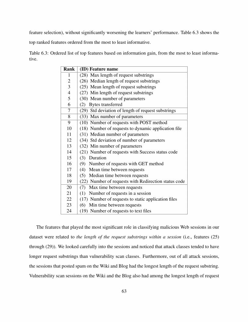
feature selection), without significantly worsening the learners’ performance. Table 6.3 shows the

top ranked features ordered from the most to least informative.

Table 6.3: Ordered list of top features based on information gain, from the most to least informa-tive.

Rank (ID) Feature name1 (28) Max length of request substrings2 (26) Median length of request substrings3 (25) Mean length of request substrings4 (27) Min length of request substrings5 (30) Mean number of parameters6 (2) Bytes transferred7 (29) Std deviation of length of request substrings8 (33) Max number of parameters9 (10) Number of requests with POST method10 (18) Number of requests to dynamic application file11 (31) Median number of parameters12 (34) Std deviation of number of parameters13 (32) Min number of parameters14 (21) Number of requests with Success status code15 (3) Duration16 (9) Number of requests with GET method17 (4) Mean time between requests18 (5) Median time between requests19 (22) Number of requests with Redirection status code20 (7) Max time between requests21 (1) Number of requests in a session22 (17) Number of requests to static application files23 (6) Min time between requests24 (19) Number of requests to text files

The features that played the most significant role in classifying malicious Web sessions in our

dataset were related to the length of the request substrings within a session (i.e., features (25)

through (29)). We looked carefully into the sessions and noticed that attack classes tended to have

longer request substrings than vulnerability scan classes. Furthermore, out of all attack sessions,

the sessions that posted spam on the Wiki and Blog had the longest length of the request substring.

Vulnerability scan sessions on the Wiki and the Blog also had among the longest length of request

63

substring.

Features (30) – (34), which dealt with the number of parameters passed in request substring

within a session, were also among the top highly ranked features based on the information gain.

This is due to the fact that our honeypot contained interactive content (i.e., ran MediaWiki and

Wordpress). In particular, exploring the values of these features in the raw data showed that attacks

which posted spam to the Wiki and Blog passed more parameters than any other attack class.

Overall, attack sessions typically passed more parameters than vulnerability scan sessions.

The feature (2) bytes transferred was among the top six features which were included in the

selected feature subset for all learners. When considered on its own, this feature showed that

some classes transfer fixed number of bytes to the server in each session. For instance, the DFind

vulnerability scan class had 43 out of 44 sessions where the number of bytes transferred was the

same (i.e., 4167).

As expected, the number of requests with POST method (i.e., feature (10)) also appeared among

the top ranked features. A close inspection of the data showed that all vulnerability scan classes

had zero requests with POST method, while attack classes had zero or more requests with POST

method. Attacks such as password cracking or posting spam on Wiki or Blog included at least one

request with POST method.

Following down the list of the top ranked features is the feature (18) number of requests to

dynamic application files (e.g., files with extension .php and .asp), which can be expected having

in mind that our servers ran dynamic content. Thus, we noticed that both vulnerability scan and

attack classes related to spam had higher number of requests to the dynamic application files than

any other class. This is because the malicious activities related to spam only work when there is

an interactive component present on the attacked system.

Feature (21) number of requests with Success status code was also included among the top

features. In our dataset, attacks typically had greater number of requests with Success status code

than vulnerability scans. This phenomenon can be attributed to the following reasons. First, as

64

discussed in our previous work [30], most of the attacks on Web systems are search-based (i.e., use

search engines or malicious crawlers to locate the application before launching the attack), that is,

attempt to exploit an existing application on our system, which results in Success status code of the

requests. On the other side, vulnerability scans often checked for particular file and/or application

which were not present on the system, resulting in an error status code (e.g., Not Found 404).

6.2.4 Using PART rules to characterize different classes of malicious Web

sessions

Tree-based learners allow for high level of interpretability of the results, thus, just as in the two-

class classification problem, we extracted PART rules. By exploring the rules produced by PART

we found that a large portion of these rules made sense. In Table 6.4 we provide several examples

of PART rules which illustrate the usefulness of the results for intrusion protection and detection

systems, such as firewalls and intrusion detection tools.

In general, some rules covered more instances than others (see Table 6.4). For example, out

of total 1,229 Spam on Blog sessions 1,218 were successfully classified using the rule shown in

Table 6.4, which classified as Spam on Blog the sessions that had at least one request with POST

method, at most one maximum number of parameters passed in a request, and median length of

request substring between 18 and 27 characters. The two different rules used to classify Spam on

Wiki given in Table 6.4 covered 662 and 83 instances respectively, out of the total 1,118 sessions

in this class. These examples show that Spam on Blog was very distinctive and, therefore almost

the whole class can be successfully classified with only one rule. On the other side, it appears

that there were different variants of session behaviors for posting Spam on Wiki, which required

different rules to be classified.

The examples in Table 6.4, in addition to large classes such as Spam on Blog and Spam on Wiki,

also include small classes such as DFind, Password cracking on Wiki and DoS. Recall that these

65

Table 6.4: PART rules examples based on using all 43 features.

PART rule Class Number of instances Class sizecovered by the rule

Number of requests with Success status code = 0 ANDMin length of requests substring > 21 ANDMedian length of requests substring <= 64 ANDBytes transferred > 2138 AND DFind 37 37Min number of parameters passed = 0 ANDNumber of requests with POST method = 0 ANDMin length of requests substring > 26 ANDMin length of requests substring <= 32Number of requests to dynamic application files = 0 ANDMax length of requests substring <= 33 AND Static 387 436Number of requests with Error status code <= 3Number of requests to static application files (.html, .htm) = 0 ANDMax length of requests substring <= 57 AND DoS 4 4Number of requests with OPTIONS method > 0Number of requests with POST method > 0 ANDMin number of parameters passed > 0 ANDNumber of requests with Error status code = 0 AND Password 48 60Standard deviation of number of parameters passed => 0.7 AND crackingNumber of requests to static application files (.html, .htm) <= 1 AND on WikiNumber of remote sites injected = 0Number of requests with POST method > 0 ANDMax number of parameters passed <= 1 AND Spam on 1,218 1,229Median length of requests substring > 18 AND BlogMedian length of requests substring <= 27Number of requests with POST method > 0 ANDMean number of parameters passed > 1.22Min length of requests substring <= 50 AND Spam on 662 1,118Number of requests to Picture files (.jpeg, .jpg, .gif) = 0 AND WikiNumber of remote sites injected = 0 ANDStandard deviation of number of parameters passed <= 1Number of requests with POST method > 0 ANDMin number of parameters passed > 0 AND Spam on 83 1,118Number of remote sites injected > 0 AND WikiStandard deviation of number of parameters passed <= 0.81

66

classes, in spite of the small size, were among the classes with the highest recall values.

6.2.5 Addressing the class imbalance problem

Our dataset was highly imbalanced, which imposed a challenge to the machine learning methods.

As discussed in section 6.2.1, the classes with lowest F-score, without exception, were very small

classes. In this section we explore the use of several methods that have potential to address the

class imbalance problem.

6.2.5.1 AdaBoost

AdaBoost algorithm [23] is a meta-algorithm used along with other learning algorithms. In par-

ticular, AdaBoost runs on the dataset several times and in each run it updates the distribution of

weights for all classes. In every round the weights of poorly classified classes are increased and

the weights of well classified classes are decreased, thus the classifier in the next run focuses on

the classes which have so far eluded correct classification. Therefore, AdaBoost is adaptive in the

sense that subsequently built classifiers are tweaked in favor of those instances misclassified by

previous classifiers.

Somewhat surprisingly, AdaBoost did not improve learners’ performance on the small mis-

classified classes for our dataset. We suspect that this result was due to the fact that our dataset

was highly imbalanced, with the smallest classes consisting only of handful of instances.

6.2.5.2 Other feature selection methods

The results presented in this work thus far were based on using information gain as a feature

selection method. Information gain, however, is known to favor features with many values over

those with a few values. That is, features with many values have high information gain and are

selected as very discriminative even though they might not be. In order to address this problem, we

67

experimented with three additional feature selection methods: information gain ratio, chi-squared,

and relief.

The information gain ratio [49] penalizes features that have many values by incorporating a

term, called spit information, that is sensitive to how broadly and uniformly a feature splits the

data. However, using the information gain ratio for feature selection on our dataset did not improve

the classification results. For example, when J48 was used with the top six features selected by the

information gain ratio method the overall accuracy dropped by almost 4% compared to the overall

accuracy achieved when information gain was used to select the top six features.

Similarly, using the chi-squared feature selection method did not improve the results. Thus, the

overall accuracy of J48 with the top six features selected by the chi-squared method was 91.93%,

which is lower than the overall accuracy of 93.77% obtained when the top six features were se-

lected by the information gain method.

We also used the relief feature selection method, which according to [64] is more stable for

imbalanced datasets than the other three previously discussed feature selection methods. However,

on our dataset the learners had the worst accuracy when using the features selected by relief. For

example, J48 had overall accuracy of 89.26%, which was lower that the accuracy with any other

feature selection method previously discussed.

Over 90% percent of the traffic was distributed among 5 classes and each of the other 14 classes

accounted for less than 1% of the whole dataset. These 14 classes are too small to significantly

effect the feature selection process. In summary, of the four feature selection methods used in

this thesis information gain led to the best classification results.

6.2.5.3 Per class feature selection approach

So far, regardless of the specific feature selection method, we used the so called simultaneous

multiclass feature selection approach which selects joint features for all classes, which often are

referred to as global features. (The top 24 global features selected using information gain are pre-

68

sented in Table 6.3.) However, when choosing these global features the feature selection method

tends to be drawn to select features for the larger classes and classes with strong predictive fea-

tures, that is, for the “easy” classes. The “difficult” classes typically contribute less than others in

the feature selection process, either because they are much smaller or have very weak predictive

features.

As the number of distinct classes increases, so does the difficulty of multiclass classification.

Some classes are inevitably more difficult to classify than others, that is, they have substantially

lower precision and/or recall compared to the other classes. Our results presented in section 6.2.1

prove this point. The reasons for poor classification of some classes may be:

1. very few positive training examples for the class, and/or

2. lack of good predictive features for that class.

Based on the results presented in section 6.2.1 the “difficult” classes in our dataset were all

very small and the poor classification is due to the case 1. We believe that this is an intrinsic

characteristic of malicious behaviors – some classes are always going to be much smaller and

obtaining more training cases for these classes would be hard.

In this section we explore the case 2 by doing per class feature selection instead of global

feature selection for all classes. In other words, we employed the one-versus-all technique with

stratified 10 cross validation on the tuning subset, where features were selected for one class versus

all other classes. We refer to these per class features as local features.

The results of this approach are detailed in Figure 6.5. The x-axis presents all 19 malicious

classes with the corresponding instances in the tuning subset in brackets. The 19 malicious classes

are ordered on x-axis by difficulty (i.e., F-score) as in Figure 6.2.

The y-axis shows the information gain scores for all 43 features, for each class individually

(i.e., the information gain of the local features). The higher the dot, the more useful that feature is

to that class. Each column has all 43 features, though in different positions.

69

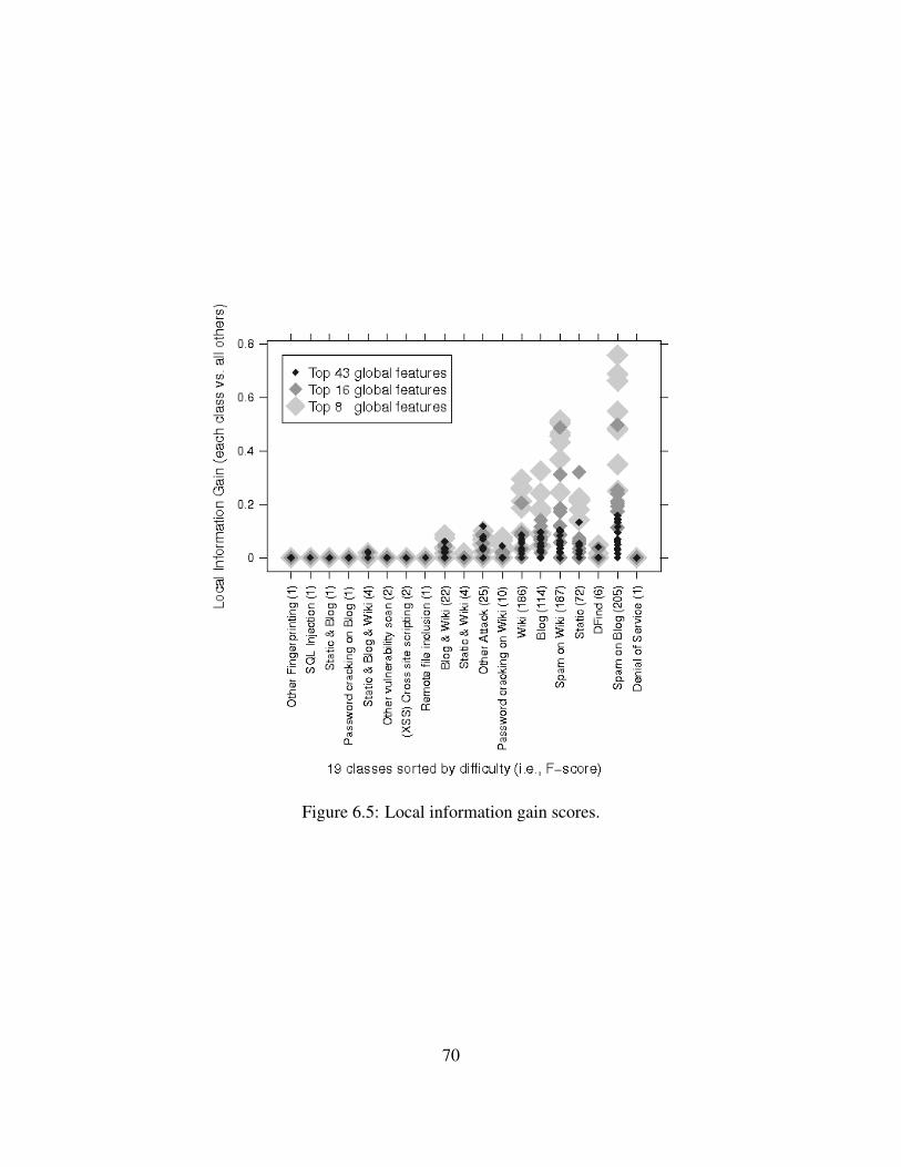
Figure 6.5: Local information gain scores.

70

To indicate the global selection order, we emboldened points in Figure 6.5 that represent top

features selected by the global feature scoring. We used different marker icons to label features

that were included in the top 8, top 16, and top 43 globally selected features. If a particular local

feature belonged to the global top 8 features it was represented by a large size, light gray diamond.

Features that belonged to the global top 16, and above global top 16 were represented by medium

size gray and small size dark diamonds, respectively. This representation allows us to view how the

global feature selection mechanism was allocating features among the classes, and which locally

predictive features it was omitting.

As expected, the best features of the five largest classes (i.e., vulnerability scan classes Static,

Blog, and Wiki and attack classes Spam on Blog and Spam on Wiki) were all selected among the top

8 or top 16 features selected globally, shown with large size, light gray diamonds or medium size,

medium gray diamonds in Figure 6.5. Notice that in general the more difficult classes toward the

left tended to have none or very few good predictive features (i.e., features with high information

gain). We further observed in Figure 6.5 that for two classes (i.e., Blog & Wiki and Other attack)

some of the better predictive features for those classes (shown with small dark diamonds) were not

selected among the top 8 or top 16 globally selected features. We used the locally selected features

from these two classes to classify the data, but no significant improvement in classification.

Another interesting observation is related to several small classes (i.e., DoS, DFind, and Pass-

word cracking Wiki) for which both locally and globally selected features did not have high predic-

tive power, but were still well classified with F-score above 90%. A close inspection of the raw data

showed that even though these classes have not contributed towards the selection of the top global

features, they all had distinct patterns for the top ranked features, which led to good classification

results. For example, all four sessions in the DoS class had the same mean, median and maximum

length of the request substrings. Moreover, the minimum length of the request substrings, which

was one character, was the smallest minimum length among all classes. The maximum length was

seven characters and it was the second smallest maximum length among all classes. In the case of

71

DFind vulnerability scan class 43 out of total 44 sessions had requests with the same length of the

request substrings (i.e., 29), the same number of bytes transferred (i.e., 4,167) and zero number of

parameters. Finally, 50 sessions out of 71 sessions in the Password cracking Wiki class followed a

pattern with same values for each of the top five features (i.e., maximum, median, mean, and mini-

mum length of the request substrings and mean number of parameters). Only the bytes transferred

(i.e., the sixth top feature) was different, likely because of different password strings.

In summary, our results showed that using the per class feature selection approach did

not improve the classification on our dataset, which is heavily imbalanced.

72

Chapter 7

Stream Semi-supervised Multi-class

Classification of Malicious HTTP Traffic

In this chapter we present the results achieved by using the concurrent stream semi-supervised

algorithm CSL-Stream on completely and partially labeled data, and compare the results to the

results of J481.

In contrast to the supervised two-class and multi-class classification, here we did not use 10

cross-validation but we trained and tested the learners on sequential chunks of the data that were

created using the arrival of the data. We chose this method in order to see whether the machine

learning algorithms were able to successfully classify the data when there was concept drift and

concept evolution present. As noted earlier, concept drift occurs when the process that is generating

the data changes over time and this leads to a high error rate in the model trying to classify the data

and concept evolution [47] refers to the discovery of novelty, i.e., classes that did not exist in the

past started to appear in the future.

In this chapter we address the following two research questions:

1. Based on accuracy, does J48 classify the data better than CSL-Stream? Based on accuracy,1Comparing the results of CSL-Stream to the results of J48 was performed only when the data were completely

labeled

73

is the classification with completely labeled data better than with partially labeled data?

2. Based on the per class metrics (i.e., Fi-Score), does J48 classify the data better than CSL-

Stream? Based on Fi-Score, is the classification with completely labeled data better than with

partially labeled data? How is classification affected by concept drift and concept evolution?

We would like to note that, unlike some of the related work [50] which used only accuracy, we

also employ the per class metrics presented in Section 6.1.2 to evaluate the learners performance

on our data, i.e., per class Recall (6.2), per class Precision (6.3), and per class Fi-Score (6.4).

In what follows we first present our data mining approach. Second, we compare the classifi-

cation of CSL-Stream to the classification of J48, using accuracy as an evaluation criteria, with

completely labeled data. Then, we discuss the results of using CSL-Stream when the window size

was 1,000 and 500 instances with different percent of labeled data. Finally, we present a discussion

of the results.

7.1 Data Mining Approach for Stream Semi-supervised Classi-

fication

In this chapter we again used the merged Web 2.0 I and Web 2.0 II datasets.

CSL-Stream is an iterative algorithm that is able to process data streams. We experimented with

two different window sizes because the window size is an adjustable parameter in CSL-Stream

which affects the classification. The data were divided first into six equally sized chunks and then

into twelve equally sized chunks, or windows as they are commonly referred in the literature [63],

[19], [32]. When the data were divided into six windows each window had exactly 1,000 instances

(the sixth window had 902 instances), whereas when the data were divided into twelve windows

each window had exactly 500 instances (the sixth window had 402 instances).

The data in each odd window were used for training the learner and the data in each even

74

window were used for testing the learner. For example, the data in the first window (Window 1

Train) were used for training the learner and the data in the second window (Window 1 Test) were

used for testing the learner. In the same context, the data in the third (Window 2 Train) window

were used for training the learner and the data in the fourth (Window 2 Test) window were used

for testing the learner. Note that the order of arrival of the data were not altered in any way, i.e.,

the first 1,000, or 500 instances depending on the window size, were included in the first window

and the second 1,000 (or 500) instances were included in the second window. The same training

and testing process was used with J48 and its classification results were compared to the results of

CSL-Stream with completely labeled data.

Besides the size of the window, there were seven other parameters which needed to be set

before learning with CSL-Stream could begin. These parameters were set to their default values,

i.e., the recommended values in [50].

Because CSL-Stream is a semi-supervised learning algorithm which is able to learn from data

that have been labeled only partially, we ran experiments when the data in each window, were

completely labeled (i.e., 100%) and partially labeled (i.e., 50% and 25%). We also ran experiments

when the data were only 10% labeled, but the classification results were not satisfactory, thus they

were not included in this thesis.

7.2 Based on accuracy, does J48 classify the data better than

CSL-Stream? Based on accuracy, is the classification with

completely labeled data better than with partially labeled

data?

In this section, using accuracy as an evaluation criteria, we answer research question one by com-

paring CSL-Stream to J48, which was the supervised algorithm that best classified our data.

75

Figure 7.1 and Figure 7.2 present the accuracy for CSL-Stream and J48, in each pair of train

and test windows, with completely and partially labeled data where the window sizes were set to

1,000 and 500 instances, respectively. When the window size was set to 1,000 instances and the

data were completely labeled the accuracy of J48 was on average 13% higher than the accuracy of

CSL-Stream with completely labeled data. With a window size of 500 instances and completely

labeled data, there was an improvement in the classification of the data for both CSL-Stream and

J48. In this case the difference in average accuracy between the two learners reduced by 3%, i.e.,

the accuracy of J48 was on average 10% higher than the accuracy of CSL-Stream. In other words,

when the data were completely labeled and the window size was reduced to 500 instances per

window, it seems that the difference in classification between CSL-Stream and J48 was not that

big, that is, in terms of accuracy, J48 classified the completely labeled data slightly better than

CSL-Stream.

Figure 7.1: Accuracy of J48 and CSL-Stream when the window size was set to 1,000 instances.The line between the accuracy values was put only for visualization purposes.

As we can see in Figure 7.1 and Figure 7.2 when the data were partially labeled, there was a

small drop in the classification accuracy.

The average accuracy when the window size was set to 1,000 instances with completely, 50%

76

Figure 7.2: Accuracy of J48 and CSL-Stream when the window size was set to 500 instances. Theline between the accuracy values was put only for visualization purposes.

and 25% labeled data was 73%, 70% and 67%, respectively. This indicates that the difference in

classification between completely and 50%, and completely and 25% labeled data was on average

3% and 6%, respectively. In the same fashion, the difference in classification between 50% and

25% labeled data was on average 3%.

When the size of the window was reduced (i.e., set to 500 instances), the average accuracy

when the data were completely, 50% and 25% improved (i.e., with a window of 500 instances the

average accuracy when the data were completely, 50% and 25% labeled was equal to 84%, 82%

and 76%, respectively). We can see that the difference in classification between completely and

50%, and completely and 25% labeled data was on average 2% and 8%, respectively. In the same

fashion, the difference in classification between 50% and 25% labeled data was on average 6%.

These results indicated that, even though CSL-Stream classified the data slightly worse than

J48 in terms of accuracy, its classification was still good with partially labeled data. Recall, that

J48 could not work with partially labeled data. When the data were 50% or even 25% labeled, the

drop in the average difference in accuracy was no worse than 8% when the data were completely

labeled. This is an important observation since labeling the data completely is very expensive, time

77

consuming, error prone and in some occasions impossible. Semi-supervised machine learning

algorithms, such as CSL-Stream, can be used to classify such partially labeled data with

insignificant degradation in accuracy.

7.3 Classification Based on the per Class Metrics (i.e., Fi-Score).

In this section, we address research question two, with two different sizes of the window, i.e., with

1,000 and 500 instances. First, using Fi-Score as an evaluation criteria, we compare CSL-Stream to

J48 with completely labeled data and also address the classification performance of CSL-Stream

on partially labeled data. Second, we study how the phenomenon of concept drift affects the

classification of the data.

7.3.1 Comparison Based on Fi-Score With a Window of 1,000 Instances

Figure 7.3 presents the average Fi-Scores, for each of the 19 malicious classes, over the three

pairs of windows with 100%, 50% and 25% labeled data. The Fi-Scores for each window are

given in Table A.1 in Appendix A. It is clear from Figure 7.3, based on average Fi-Scores, that

J48 classified the completely labeled data better than CSL-Stream. The lowest difference in

average Fi-Scores between J48 and CSL-Stream was 6% in the Blog & Wiki class, and the highest

difference was 28% in the Static class. Furthermore, 10 out of 19 classes had average Fi-Scores

different than 0% when CSL-Stream was used, and 11 out of 19 classes had average Fi-Scores

different than 0% when J48 was used. If we consider average Fi-Score, over the three pairs of

windows, greater than 50% to be good classification, among the 10 classified classes by CSL-

Stream only 6 have average Fi-Score greater than 50%, where as when J48 was used, 9 classes had

Fi-Score greater than 50%.

Figure 7.4 presents the difference in average per class Fi-Scores for each of the 19 classes with

100% and 50% labeled data, 100% and 25% labeled data, and 50% and 25% labeled data. The

78

Figure 7.3: Fi-Scores averaged, for each of the 19 malicious classes, over the three pairs of win-dows with 100%, 50% and 25% labeled data. The average Fi-Scores of J48 with completely labeleddata are also included. In each window there were 1,000 instances. The classes are ordered fromleft to right based on the average Fi-Scores of J48. The line between the Fi-Scores values was putonly for visualization purposes.

lowest and greatest difference in classification when the data were completely labeled as opposed

to 50% labeled, were -2% and 13% respectively. Here a negative value means that the average

Fi-Scores with 50% labeled data was better than the average Fi-Scores with completely labeled

data for that class. Similarly the lowest and greatest difference in classification when the data

were completely labeled as opposed to 25% labeled, was -2% and 8%, respectively. When we

considered the lowest and greatest difference in average per class Fi-Scores with 50% and 25%

labeled data we got -11% and 2%, respectively, which means that the data were classified better

when 25% were labeled then when 50% were labeled.

Table 7.1 presents the mean and standard deviation of the difference in Fi-scores averaged

across the three pairs of windows between completely and partially labeled data. We can see that

the mean difference in Fi-scores averaged across the three pairs of windows between completely

and partially labeled data does not exceed 2% with a standard deviation of 4%.

79

Table 7.1: Mean and standard deviation of the difference in Fi-scores, averaged across the threepairs of windows, between completely and partially labeled data.

100% and 50% labeled 100% and 25% labeled 50% and 25% labeled

Mean 2% 1% -1%Standard Deviation 4% 3% 3%

Based on per class Fi-Scores it appears that CSL-Stream classified the partially labeled

data (i.e., 25% and 50%) as good as the completely labeled data. As we previously noted, this

is an important observation since labeling the data completely is a very expensive, time consuming,

error prone and in some occasions impossible process.

Figure 7.4: Differences in the average per class Fi-Scores, over the three pairs of windows, between100% and 50% labeled data, 100% and 25% labeled data, and 50% and 25% labeled data.

Nine classes with CSL-Stream and eight classes with J48, that appear on the left side of the

x-axis on Figure 7.3 were not classified at all, i.e., the average Fi-Scores for these classes was

0%. The reason why these classes were not classified, is because they were very small, together

80

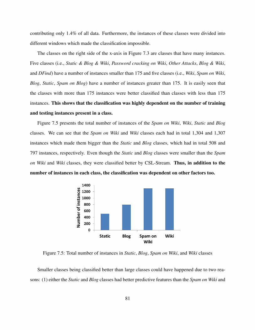
contributing only 1.4% of all data. Furthermore, the instances of these classes were divided into

different windows which made the classification impossible.

The classes on the right side of the x-axis in Figure 7.3 are classes that have many instances.

Five classes (i.e., Static & Blog & Wiki, Password cracking on Wiki, Other Attacks, Blog & Wiki,

and DFind) have a number of instances smaller than 175 and five classes (i.e., Wiki, Spam on Wiki,

Blog, Static, Spam on Blog) have a number of instances greater than 175. It is easily seen that

the classes with more than 175 instances were better classified than classes with less than 175

instances. This shows that the classification was highly dependent on the number of training

and testing instances present in a class.

Figure 7.5 presents the total number of instances of the Spam on Wiki, Wiki, Static and Blog

classes. We can see that the Spam on Wiki and Wiki classes each had in total 1,304 and 1,307

instances which made them bigger than the Static and Blog classes, which had in total 508 and

797 instances, respectively. Even though the Static and Blog classes were smaller than the Spam

on Wiki and Wiki classes, they were classified better by CSL-Stream. Thus, in addition to the

number of instances in each class, the classification was dependent on other factors too.

Figure 7.5: Total number of instances in Static, Blog, Spam on Wiki, and Wiki classes

Smaller classes being classified better than large classes could have happened due to two rea-

sons: (1) either the Static and Blog classes had better predictive features than the Spam on Wiki and

81

Wiki classes or (2) the distribution of the Static and Blog classes in each training and testing win-

dow was more stable (i.e., the concept drift was smaller) than the Spam on Wiki and Wiki classes.

From the ’Per Class Feature Selection Approach’ section in Chapter 6 we know that these classes

share the same most predictive features, thus the reason why the smaller classes were classified

better than the bigger classes must be due to concept drift.

In order to explore how the classification is affected by concept drift we present Figure 7.6

which gives the distribution of instances in each training and testing window by class, with 1,000

instances in each window. Based on Figure 7.6 we managed to identify four different scenarios of

concept drift.

1. Classes that appeared in all windows with different degree of concept drift. This scenario

included the classes Cross-site scripting, Blog & Wiki, Blog, Spam on Wiki, Wiki, Static, and

Spam on Blog.

2. Classes that existed in the past, seized to exist and appeared again in the future. This scenario

included the classes DFind, Static & Blog, Static & Wiki, Static & Blog & Wiki, Remote File

Inclusion and Password cracking on Blog.

3. Classes that did not exist in the past, started to exist in the future, i.e., classes that exhibited

concept evolution rather than concept drift. This scenario included the Other Fingerprinting

class. The Other Vulnerability Scan, Other Attacks and Password cracking on Wiki classes

are included in this scenario too, because they did not have any instances only in the first

window.

4. Classes that existed in the past, seized to exist in the future. This scenario included the

classes Denial of Service and SQL Injection.

For the first scenario, the only class which was not classified well was the Cross-site scripting

class and this happened because the Cross-site scripting class was very small, contributing only

82

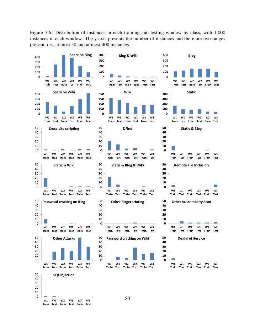
Figure 7.6: Distribution of instances in each training and testing window by class, with 1,000instances in each window. The y-axis presents the number of instances and there are two rangespresent, i.e., at most 50 and at most 400 instances.

83

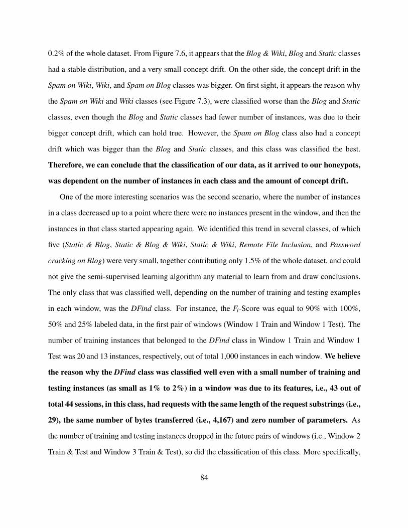
0.2% of the whole dataset. From Figure 7.6, it appears that the Blog & Wiki, Blog and Static classes

had a stable distribution, and a very small concept drift. On the other side, the concept drift in the

Spam on Wiki, Wiki, and Spam on Blog classes was bigger. On first sight, it appears the reason why

the Spam on Wiki and Wiki classes (see Figure 7.3), were classified worse than the Blog and Static

classes, even though the Blog and Static classes had fewer number of instances, was due to their

bigger concept drift, which can hold true. However, the Spam on Blog class also had a concept

drift which was bigger than the Blog and Static classes, and this class was classified the best.

Therefore, we can conclude that the classification of our data, as it arrived to our honeypots,

was dependent on the number of instances in each class and the amount of concept drift.

One of the more interesting scenarios was the second scenario, where the number of instances

in a class decreased up to a point where there were no instances present in the window, and then the

instances in that class started appearing again. We identified this trend in several classes, of which

five (Static & Blog, Static & Blog & Wiki, Static & Wiki, Remote File Inclusion, and Password

cracking on Blog) were very small, together contributing only 1.5% of the whole dataset, and could

not give the semi-supervised learning algorithm any material to learn from and draw conclusions.

The only class that was classified well, depending on the number of training and testing examples

in each window, was the DFind class. For instance, the Fi-Score was equal to 90% with 100%,

50% and 25% labeled data, in the first pair of windows (Window 1 Train and Window 1 Test). The

number of training instances that belonged to the DFind class in Window 1 Train and Window 1

Test was 20 and 13 instances, respectively, out of total 1,000 instances in each window. We believe

the reason why the DFind class was classified well even with a small number of training and

testing instances (as small as 1% to 2%) in a window was due to its features, i.e., 43 out of

total 44 sessions, in this class, had requests with the same length of the request substrings (i.e.,

29), the same number of bytes transferred (i.e., 4,167) and zero number of parameters. As

the number of training and testing instances dropped in the future pairs of windows (i.e., Window 2

Train & Test and Window 3 Train & Test), so did the classification of this class. More specifically,

84

in the second and third pair of windows there were 4 and 0 training instances, and 5 and 2 testing

instances, respectively, resulting in Fi-Scores of 59% (with 100%, 50% and 25% labeled data) and

0% (with 100%, 50% and 25% labeled data), respectively. Even thought the classification of this

class in some windows was very good the average classification over the three windows was low

(Fi-Score was equal to 50%) due to the bad classification in the other windows.

In the third scenario we have four cases where concept evolution or discovery of novelty was

present, i.e., classes that did not exist in the past started to appear in the future. This is an every

day scenario in real world Web servers, which are being attacked by new attacks on regular basis.

Two classes (Other Attacks and Password cracking on Wiki) in the third scenario had average

Fi-Scores different than 0%. The Fi-Score recorded for these two classes was equal to 0% when the

learner was trained on Window 1 Train and tested on Window 1 Test2. This happened because there

were no instances present to train on in Window 1 Train, but there were instances present, of these

two classes, to test on in Window 1 Test. Since the learner had not been trained to recognize these

classes, it missclassified them. However, as the number of training and testing instances increased,

so did the Fi-Scores (i.e., classification improved), especially for the Password cracking on Wiki

class. It appears that CSL-Stream could not detect the novelty when it first appeared, but it

was able to recognize and classify the novelty if it prevailed in future windows. The other two

classes (Other Fingerprinting and Other Vulnerability Scan) had only a handful of instances (i.e.,

together contributed only 0.2% of the whole dataset) which were not enough for the algorithm to

learn and retrieve useful information. Therefore, the classification in these two classes was very

poor (i.e., the Fi-Scores were equal to 0%).

The classes that belong to the fourth scenario, Denial of Service and SQL Injection, had

in total four and two instances, respectively, which were not enough to make any solid claims

about the performance of CSL-Stream, and its response to concept drift. In both cases, for

Denial of Service and SQL Injection, the reported Fi-Score was 0%. It is probably interesting to

2The Fi-Scores for each window are given in Table A.1 in Appendix A

85

note that in Window 1 Train there were four instances of the Denial of Service class used to train

the learner and then the learner was tested on zero Denial of Service instances in W1 Test window.

In summary, based on average Fi-Scores, over the three pairs of windows, J48 classified the

data better than CSL-Stream but CSL-Stream was able to classify the partially labeled (i.e., 25%

and 50%) data as good as when it was completely labeled. Furthermore, the classification of the

bigger classes depends on the arrival of instances (i.e., concept drift), the number of instances per

class in each window and the distinctive features of each class.

7.3.2 Comparison Based on Fi-Scores With a Window of 500 Instances

Since the size of the window is an adjustable parameter that can affect the classification of CSL-

Stream, in this section we reduce the size of the window to 500 instances and see if CSL-Stream

can classify the data better with a smaller window than with a bigger window. A small window

has the potential to create a very accurate model when there is a big concept drift in the data, while

a larger window is beneficial when the data generation process is stable (i.e., the distribution of

classes does not change much) [66], [38].

Figure 7.7 presents the Fi-Scores averaged over the six pairs of windows with 100%, 50% and

25% labeled data. The Fi-Scores for each window are given in Table A.2 in Appendix A. Similarly

as when the window size was 1,000 instances, J48 classified the completely labeled data, with

500 instances per window better than CSL-Stream. Nine classes with CSL-Stream and eight

classes with J48, which appear on the left side of the x-axis on Figure 7.7 were not classified at all,

i.e., the Fi-Scores over the 6 pairs of windows for these classes were 0%. Similarly as when the

window size was 1,000 instances, the reason why these classes were not classified at all, is because

they were very small, together contributing only 1.4% of all the data. Even more, the instances

of these classes were divided into different windows which made these classes even smaller and

even more difficult to learn from. The lowest difference in average Fi-Scores between J48 and

CSL-Stream was -6% in the Spam on Wiki class, and the highest difference was 45% in the Other

86

attacks class. Furthermore, 10 out of 19 classes had average Fi-Scores different than 0% when

CSL-Stream was used, and 11 out of 19 classes had average Fi-Scores different than 0% when J48

was used. If we consider average Fi-Scores greater than 50% to be good classification, among the

10 classified classes by CSL-Stream only 7 , when the data was completely and 50% labeled, and

6 when the data was 25% labeled had average Fi-Score greater than 50%. Similarly, when J48 was

used, 8 classes had Fi-Scores greater than 50%.

The smaller window improved the average Fi-Scores for some classes (DFind, Password crack-

ing on Wiki, Wiki, Static, Blog, and Spam on Wiki), while for other classes the average Fi-Scores

worsened (Static & Blog & Wiki, Other Attacks, Blog & Wiki, and Spam on Blog). Depending on

the amount of labeled data, in some classes the average Fi-Score improved by at most 23% (i.e.,

Password cracking on Wiki with completely labeled data) and in other classes worsened by at most

30% (i.e, Blog & Wiki with 25% labeled data).

Figure 7.7: Fi-Scores averaged, for each of the 19 malicious classes, over the six pairs of windowswith 100%, 50% and 25% labeled data. In each window there were 500 instances. The averageFi-Scores of J48 with completely labeled data are also included. The classes are ordered from leftto right based on the average Fi-Scores of J48. The line between the Fi-Scores values was put onlyfor visualization purposes.

87

In order to answer the question why the average Fi-Scores worsened, while for some classes

improved, we present Figure 7.8 which depicts the distribution of instances in each class in the 6

pairs of windows. We now address each class and elaborate why its average Fi-Score worsened or

improved.

We start with the four classes whose Fi-Scores improved.

For the group of classes whose average classification improved, two classes (i.e., DFind con-

tributed 0.7% and Password cracking on Wiki contributed 1.2% of the whole dataset) were very

small and four classes (Wiki, Static, Blog, and Spam on Wiki) were bigger.

The classification of the four big classes improved because with a smaller window there were

more windows where CSL-Stream learned and was tested. In other words, because of the extra

training and testing windows with varying, but sufficient, number of instances CSL-Stream was

able to learn that these classes were present all the time. Thus, CSL-Stream tuned its model to

favor instances of these four classes for classification. Table 7.2 presents the increase in average

per class Fi-Scores when the window width was decreased from 1,000 to 500 instances with 100%,

50% and 25% labeled data. The biggest increase in average Fi-Scores, over the 6 pairs of windows,

among these four big classes was by 20% in the Spam on Wiki class with completely labeled data.

Note that the -14% Fi-Score in the Static class with 25% labeled data indicates that the classification

with window size of 1,000 instances was better then the classification when the window size was

set to 500 instances.

The slight improvement of 2% and 3% in the average Fi-Scores of the DFind class, was due

to the smaller window size, in Window 4 and Window 6. The Fi-score was equal to 80% and

100% in Window 4 and Window 6, respectively, which improved the average Fi-Scores by 2% and

3%. Similarly the Fi-Scores of the Password cracking on Wiki class improved by 23%, 8% and

13% with completely, 50% and 25% labeled data, respectively. The improvement in the average

Fi-Scores of this class was due to the better classification in Windows 3, 4, 5, and 6.

Table 7.3 presents the decrease in average per class Fi-Scores, averaged across all pairs of

88

Figure 7.8: Distribution of instances in each training and testing window by class, with 500 in-stances in each window. The y-axis presents the number of instances and there are two rangespresent, i.e., at most 60 and at most 200 instances.

89

Table 7.2: Increase in per class Fi-Scores averaged across all pairs of windows when the windowwidth was decreased from 1,000 to 500 instances with 100%, 50% and 25% labeled data.

Class 100 % labeled 50% labeled 25% labeled

DFind 2% 2% 3%Password cracking on Wiki 23% 8% 13%Wiki 13% 12% 9%Static 6% 5% -14%Blog 5% 11% 5%Spam on Wiki 20% 19% 11%

Table 7.3: Decrease in per class Fi-Scores averaged across all pairs of windows when the windowwidth was decreased from 1,000 to 500 instances with 100%, 50% and 25% labeled data.

Class 100 % labeled 50% labeled 25% labeled

Static & Blog 8% 9% 7%Other Attacks 17% 8% 17%Blog & Wiki 3% 18% 30%Spam on Blog 6% 6% 11%

windows, when the window width was decreased from 1,000 to 500 instances with 100%, 50%

and 25% labeled data. For the three small classes (i.e., Static & Blog & Wiki, Other Attacks, Blog

& Wiki) in this group, the average classification reduced because the number of training examples

of these classes in each window reduced significantly, leading to smaller Fi-Scores in each pair of

train and test windows which reduced the average Fi-Scores of the three classes. In these three

classes, the biggest drop in the average per class Fi-Score over the six pairs of windows was in the

Blog & Wiki class with 25% labeled data, and the smallest drop was in the same class with 100%

labeled data. The average Fi-Score for the big class (i.e., Spam on Blog) in this group, worsened

by at most 11% with 25% labeled data because of the smaller number of training instances in the

first two windows (see the bottom of Figure 7.8).

It appears that the classification of the data followed a similar pattern with a window size of

500 and 1,000, with some improvement and deterioration in individual classes. Also when the

window size was reduced to 500 instances the same four concept drift scenarios appeared as when

90

the window size was 1,000 instances.

7.4 Discussion

In this section we will summarize the observations we made using CSL-Stream on our data with a

window size of 1,000 and 500 instances and formally answer the two research questions posed in

the beginning of this chapter. After answering each question we briefly compare our results to the

results of the related work on semi-supervised classification.

Regarding the first research question (i.e., Based on accuracy, does J48 classify the data better

than CSL-Stream? Based on accuracy, is the classification with completely labeled data better than

with partially labeled data?) we claim the following:

1. In terms of accuracy, the best supervised algorithm in this thesis (i.e., J48) was slightly better

than CSL-Stream with completely labeled data.

2. Based on accuracy the classification with partially labeled data was almost as good as the

classification with completely labeled data, i.e., the biggest drop in the average difference in

accuracy was 8%.

Using CSL-Stream the highest average accuracy across all the windows was equal to 84%

when the data were completely labeled and the window size was set to 500 instances. Similarly,

the lowest average accuracy across all the windows was equal to 67% when the data were 25%

labeled and the window size was set to 1,000 instances.

The related work in stream algorithms reported higher average accuracy. For instance, the

authors in [50] reported average accuracy equal to 98.06% and 85.33% with CSL-Stream and Sm-

SCluster learners, respectively, using a window of size 1,000 instances on the completely labeled

KDD Cup 1999 dataset. Even when the data were partially labeled (i.e., 50%, 25%, 10%) the

accuracy did not go below 95%. The better accuracy in [50] was due to the fact that the data were

91

completely labeled. Similarly, the authors of the SmSCluster algorithm in [46] reported average

accuracy in the range of 96-99% with a window size of 1,600 instances on 5% labeled data. It is

very important here to note that these algorithms have been used on datasets that are about 1,000

times bigger than ours. Furthermore, the authors in the related work on stream semi-supervised

algorithms evaluated their learners based on accuracy which can be a misleading metric when the

dataset is skewed, and as a matter of fact, the KDD Cup 1999 data is skewed. In order to see how

the classification works on the small classes we used the performance metrics from Chapter 6.

The related work in batch semi-supervised algorithms reported overall accuracy results similar

to ours. For instance, the authors in [59] reported highest overall accuracy of 88% with 65% labeled

data on a two class balanced dataset. We would like to note, that our dataset with 19 classes was

very skewed where 5 classes constituted 90% of the data. The authors in [14] used the KDD Cup

1999, and had training and testing datasets with different distributions. They reported an overall

accuracy of 53% without providing the percentage of label data used.

Regarding the second research question (i.e., Based on the per class metrics (i.e., Fi-Score),

does J48 classify the data better than CSL-Stream? Based on Fi-Scores, is the classification with

completely labeled data better than with partially labeled data? How is classification affected by

concept drift and concept evolution?) we claim the following:

1. In terms of per class metrics (i.e., Fi-Scores), the best supervised algorithm in this thesis

(i.e., J48) was slightly better than CSL-Stream with completely labeled data. Based on

the per class metrics (i.e., Fi-Scores) the classification with partially labeled data was as

good as the classification with completely labeled data, i.e., the mean difference in Fi-scores

averaged across the three pairs of windows between completely and partially labeled data

did not exceed 2% with a standard deviation of 4%. This is a very important observation

since labeling the data is a very long, expensive and error prone process.

2. It appears that CSL-Stream could not detect the appearance of novelty when the novelty

92

came, but CSL-Stream was able to recognize and classify the novelty if it prevailed in future

windows.

3. The classification of the bigger classes depends on the arrival of instances (i.e., concept drift),

the number of instances per class in each window and the distinctive features of each class.

4. Regardless of the window size, the difference in classification was very small with com-

pletely and partially labeled

Of the related works which used metrics different than accuracy was one stream semi-supervised

paper [47] and two batch semi-supervised papers [16], [62].

The authors in [47] were concerned with the detection of novelty and used three metrics to

evaluate the learner used in [47]. The three metrics were: (1) percent of novel class instances

misclassified as existing class, (2) percent of existing class instances falsely identified as novel

class, and (3) Total misclassification error. Unfortunately, we cannot compare our results to the

results of this paper since we used different metrics.

The two papers on batch semi-supervised learning [16], [62] studied the problem of intrusion

detection and therefore used probability of detection (i.e., recall) as an evaluation metric. They

tried to determine if a user session was legitimate or not (i.e., intruder). The recall in this case gives

the probability that an actual intrusion was detected by the system versus false alarm that gives the

probability of an legitimate user marked as an intruder by the system. In [16] on the previously

balanced DARPA dataset a recall of 86% with 10% labeled data was reported. Similarly, in [62]

recall of 64% to 96%, depending on the algorithm used, was reported on a two class dataset using

10 cross validation.

The weighted recall when the window size was set to 1,000 instances and the data were com-

pletely, 50% and 25% labeled was equal to 70.62%, 66.39% and 68.11%, respectively. Similarly,

weighted recall when the window size was set to 500 instances and the data were completely, 50%

and 25% labeled was equal to 76.43%, 72.05% and 67.37%, respectively

93

The weighted recall was defined in Section 6.1.2 equation 6.6 in Chapter 6. This performance

metric takes into account the frequency of each class in computing the average recall for all classes.

The weighted recall reduces to arithmetic average metrics if all classes are given the same weight.

94

Chapter 8

Conclusion

This work was motivated by the numerous exploits that happen every day to the Web systems

that run Web 2.0 applications. Many companies, as well as individuals, rely on the security of

these systems and reliability of Web 2.0 applications to have their businesses operate in a normal

pattern. In order to study more closely the attacks on of Web applications, this thesis used four

datasets for classification of malicious traffic. They had been collected from three high interaction

honeypots, with meaningful functionality. The datasets consisted of only malicious traffic and

were completely labeled. Each session in the datasets was characterized by a vector of 43 features

(i.e., 43 attributes characterizing a malicious HTTP session).

We first used batch supervised machine learning algorithms on our four datasets. Since our data

was labeled into two major groups, attacks and vulnerability scans, and also further labeled in nine

subgroups of attacks and eleven subgroups of vulnerability scans, we performed both, two-class

and multi-class classification.

The results of the classification of the malicious traffic using the batch two-class and multi-class

supervised machine learning algorithms show that:

• Supervised machine learning methods can be used to separate malicious HTTP traffic into

two classes (i.e., attacks and vulnerability scans) with very high probability of detection and

95

very low probability of false alarm.

• Furthermore, supervised machine learning methods can be used to separate malicious traffic

to multiple classes with high recall and precision for all but several very small classes.

• Decision tree based algorithms (i.e., J48 and PART) distinguished between attacks and vul-

nerability scans, better than the Support Vector Machines (i.e.,SVM) algorithm.

• Decision tree based algorithms (i.e., J48 and PART) distinguished among multiple mali-

cious classes better than the other three algorithms (Support Vector Machines, Multi-Layer

Perceptron and Naive Bayes Learner) and also provided better interpretability of the results.

• Since our dataset (i.e., the merged Web 2.0 dataset from Web 2.0 I and Web 2.0 II) was

heavily imbalanced, we tried three methods (i.e., AdaBoost, Other feature selection meth-

ods, and Per class feature selection) that address the class imbalance problem to improve

the multiclass classification. However, neither of these methods improved the classification

results.

• Depending on which dataset and what machine learning algorithm was used, from four to six

features were needed to classify malicious activities without significantly worsening learners

performance compared to when all 43 features were used. Specifically, the WebDBAdmin I,

WebDBAdmin II, Web 2.0 I and Web 2.0 II datasets needed four, six, four, and six features,

respectively. The merged Web 2.0 dataset, from Web 2.0 I and Web 2.0 II datasets, needed

six features when J48 was used to classify the data. These results indicate that attacks differ

from vulnerability scans only in a small number of features (i.e., session characteristics).

Since data labeling is a very expensive process, we used a stream semi-supervised machine

learning algorithm, called CSL-Stream, to classify the data. CSL-Stream uses a fading model to

respond to concept drift.

96

The results of the analysis of the malicious traffic using the stream semi-supervised machine

learning algorithms showed that:

• With completely labeled data, in terms of accuracy, the best supervised algorithm in this

thesis (i.e., J48) was slightly better than CSL-Stream .

• Using CSL-Stream and accuracy as an evaluation metric the classification with partially

labeled data (i.e., 50% and 25%) was almost as good as the classification with completely

labeled data, i.e., the biggest drop in the average difference in accuracy was 8%.

• In terms of per class metrics (i.e., F-Score), the best supervised algorithm in this thesis (i.e.,

J48) was slightly better than CSL-Stream with completely labeled data. Using CSL-Stream

and the per class metrics (i.e., F-Score) the classification with partially labeled data was as

good as the classification with completely labeled data, i.e., the mean difference in F-scores

averaged across the three pairs of windows between completely and partially labeled data

did not exceed 2% with a standard deviation of 4%. This is a very important observation

since labeling the data is a very long, expensive and error prone process.

• The classification of the bigger classes depended on the number of instances per class in

each window, the distinctive features of each class, and the arrival of instances (i.e., concept

drift),

• It appears that CSL-Stream could not detect the appearance of novelty when the novelty

came, but CSL-Stream was able to recognize and classify the novelty if it prevailed in future

windows.

• Regardless of the window size (i.e., a window of size 1,000 or 500 instances), the difference

in classification was very small with completely and partially labeled data. For some classes

the average classification improved while for others it worsened.

97

The results presented in this thesis enrich the empirical evidence on malicious cyber activities

and can support areas such as generation of attack signatures and developing models for attack

injection that can be used for testing the resilience of services and systems.

The future work will be focused on studying the temporal dependencies in malicious traffic and

use of other semi-supervised algorithms for classification.

98

Appendix A

Tables for semi-supervised learning

Table A.1: Fi-Scores values with 100%, 50% and 25% labeled data. J48 was trained and tested on100% labeled data. In each window there were 1,000 instances.

Window 1 Window 2 Window 3Train & Test Train & Test Train & Test

Amount of labeled data J48 100% 50% 25% J48 100% 50% 25% J48 100% 50% 25%Other Fingerprinting 0% 0% 0% 0% 0% 0% 0% 0% 0% 0% 0% 0%Static & Blog 0% 0% 0% 0% 0% 0% 0% 0% 0% 0% 0% 0%Static & Wiki 0% 0% 0% 0% 0% 0% 0% 0% 0% 0% 0% 0%Other Vulnerability Scan 0% 0% 0% 0% 0% 0% 0% 0% 0% 0% 0% 0%Denial of Service 0% 0% 0% 0% 0% 0% 0% 0% 0% 0% 0% 0%Password cracking on Blog 0% 0% 0% 0% 0% 0% 0% 0% 0% 0% 0% 0%Remote File Inclusion 0% 0% 0% 0% 0% 0% 0% 0% 0% 0% 0% 0%SQL injection 0% 0% 0% 0% 0% 0% 0% 0% 0% 0% 0% 0%Cross-site scripting 0% 0% 0% 0% 0% 0% 0% 0% 44% 0% 0% 0%Static & Blog & Wiki 59% 31% 32% 27% 0% 0% 0% 0% 0% 0% 0% 0%Password cracking on Wiki 0% 0% 0% 0% 69% 19% 19% 0% 96% 75% 75% 81%Other Attacks 0% 0% 0% 0% 80% 46% 18% 40% 85% 42% 43% 45%Blog & Wiki 79% 59% 55% 59% 54% 50% 36% 55% 40% 47% 38% 47%DFind 100% 90% 90% 90% 100% 59% 59% 59% 0% 0% 0% 0%Wiki 76% 73% 75% 71% 85% 57% 53% 52% 72% 57% 38% 40%Spam on Wiki 72% 65% 64% 64% 88% 69% 69% 67% 84% 70% 65% 61%Blog 74% 65% 64% 63% 90% 82% 74% 82% 88% 81% 52% 60%Static 96% 75% 76% 75% 96% 62% 61% 71% 100% 72% 79% 80%Spam on Blog 99% 96% 93% 97% 100% 95% 96% 97% 100% 88% 87% 94%

99

Table A.2: Fi-Scores values with 100%, 50% and 25% labeled data. J48 was trained and tested on100% labeled data. In each window there were 500 instances.

Win

dow

1W

indo

w2

Win

dow

3W

indo

w4

Win

dow

5W

indo

w6

Test

&Tr

ain

Test

&Tr

ain

Test

&Tr

ain

Test

&Tr

ain

Test

&Tr

ain

Test

&Tr

ain

J48

100%

100%

50%

25%

J48

100%

100%

50%

25%

J48

100%

100%

50%

25%

J48

100%

100%

50%

25%

J48

100%

100%

50%

25%

J48

100%

100%

50%

25%

Oth

erFi

nger

prin

ting

0%0%

0%0%

0%0%

0%0%

0%0%

0%0%

0%0%

0%0%

0%0%

0%0%

0%0%

0%0%

Stat

ic&

Blo

g0%

0%0%

0%0%

0%0%

0%0%

0%0%

0%0%

0%0%

0%0%

0%0%

0%0%

0%0%

0%St

atic

&W

iki

0%0%

0%0%

0%0%

0%0%

0%0%

0%0%

0%0%

0%0%

0%0%

0%0%

0%0%

0%0%

Oth

erVu

lner

abili

tySc

an0%

0%0%

0%0%

0%0%

0%0%

0%0%

0%0%

0%0%

0%0%

0%0%

0%0%

0%0%

0%D

enia

lofS

ervi

ce0%

0%0%

0%0%

0%0%

0%0%

0%0%

0%0%

0%0%

0%0%

0%0%

0%0%

0%0%

0%Pa

ssw

ord

crac

king

onB

log

0%0%

0%0%

0%0%

0%0%

0%0%

0%0%

0%0%

0%0%

0%0%

0%0%

0%0%

0%0%

Rem

ote

File

Incl

usio

n0%

0%0%

0%0%

0%0%

0%0%

0%0%

0%0%

0%0%

0%0%

0%0%

0%0%

0%0%

0%SQ

Lin

ject

ion

0%0%

0%0%

0%0%

0%0%

0%0%

0%0%

0%0%

0%0%

0%0%

0%0%

0%0%

0%0%

Stat

ic&

Blo

g&

Wik

i68

%12

%12

%12

%33

%0%

0%0%

0%0%

0%0%

0%0%

0%0%

0%0%

0%0%

0%0%

0%0%

Cro

ss-s

itesc

ript

ing

0%0%

0%0%

0%0%

0%0%

0%0%

0%0%

0%0%

0%0%

66%

0%0%

0%10

0%0%

0%0%

DFi

nd82

%71

%71

%75

%93

%61

%61

%61

%0%

0%0%

0%10

0%80

%80

%80

%0%

0%0%

0%0%

100%

100%

100%

Blo

g&

wik

i89

%65

%53

%30

%80

%55

%38

%33

%33

%67

%40

%60

%50

%67

%0%

0%20

%0%

0%0%

61%

40%

22%

22%

Pass

wor

dcr

acki

ngon

Wik

i0%

0%0%

0%10

0%0%

0%0%

67%

86%

0%0%

16%

86%

86%

86%

61%

77%

77%

77%

92%

75%

75%

75%

Oth

erA

ttac

ks0%

0%0%

0%34

%0%

0%0%

81%

14%

14%

14%

70%

0%0%

0%89

%59

%59

%55

%67

%0%

0%0%

Spam

onW

iki

99%

97%

97%

96%

88%

85%

85%

79%

70%

80%

62%

46%

44%

94%

93%

69%

91%

79%

78%

77%

94%

92%

92%

85%

Wik

i94

%86

%86

%87

%85

%78

%73

%76

%94

%79

%70

%75

%93

%66

%56

%74

%79

%65

%54

%52

%86

%78

%62

%73

%B

log

81%

55%

62%

46%

91%

85%

79%

82%

93%

85%

83%

72%

97%

89%

84%

83%

96%

93%

88%

87%

90%

80%

52%

68%

Spam

onB

log

78%

48%

42%

44%

100%

97%

96%

95%

99%

98%

97%

97%

99%

92%

91%

91%

99%

92%

95%

93%

100%

96%

96%

92%

Stat

ic96

%76

%60

%56

%98

%81

%81

%69

%97

%78

%82

%74

%10

0%70

%78

%71

%95

%63

%72

%46

%10

0%86

%87

%54

%

100

Bibliography

[1] Daily’s dave vulnerability disclosure list. www.immunitysec.com.

[2] A practical guide to support vector machine. www.csie.ntu.edu.tw/˜cjlin/papers/

guide/guide.pdf.

[3] Propfind. http://www.securityfocus.com/bid/7735/discuss.

[4] SANS, Dec 2012. http://www.sans.org/reading-room/analysts-program/

sans-survey-appsec.

[5] Security focus. http://www.securityfocus.com/.

[6] arachnids: Advanced reference archive of current heuristics for network intrusion detection

systems. www.whitehats.com/ids, 2004.

[7] Charu C Aggarwal, Jiawei Han, Jianyong Wang, and Philip S Yu. A framework for clustering

evolving data streams. In Proceedings of the 29th international conference on Very large data

bases-Volume 29, pages 81–92, 2003.

[8] Magnus Almgren, Herve Debar, and Marc Dacier. A lightweight tool for detecting Web

server attacks. In ISOC Symposium on Network and Distributed Systems Security, pages

157–170, 2000.

101

[9] Goce Anastasovski, Katerina Goseva-Popstojanova, and Risto Pantev. Behavior-based mul-

ticlass classification of vulnerability scans and cyber attacks aimed at Web 2.0 systems. Sub-

mitted to a journal, 2013.

[10] Bernhard E Boser, Isabelle M Guyon, and Vladimir N Vapnik. A training algorithm for

optimal margin classifiers. In 5th Annual Workshop on Computational Learning Theory,

pages 144–152, 1992.

[11] Greg Buehrer, Jack W Stokes, Kumar Chellapilla, and John C Platt. Classification of auto-

mated Web traffic. Chapter in Weaving Services and People on the World Wide Web, Springer

Verlag, 2007.

[12] Feng Cao, Martin Ester, Weining Qian, and Aoying Zhou. Density-based clustering over an

evolving data stream with noise. In Proceedings of the 2006 SIAM International Conference

on Data Mining, pages 328–339, 2006.

[13] Chien-Chung Chang, Hsing-Kuo Pao, and Yuh-Jye Lee. An RSVM based two-teachers–one-

student semi-supervised learning algorithm. Neural Networks, 25:57–69, 2012.

[14] Chuanliang Chen, Yunchao Gong, and Yingjie Tian. Semi-supervised learning methods for

network intrusion detection. In IEEE International Conference on Systems, Man and Cyber-

netics, 2008. SMC 2008., pages 2603–2608. IEEE, 2008.

[15] Yixin Chen and Li Tu. Density-based clustering for real-time stream data. In Proceedings of

the 13th ACM SIGKDD international conference on Knowledge discovery and data mining,

pages 133–142. ACM, 2007.

[16] Chien-Yi Chiu, Yuh-Jye Lee, Chien-Chung Chang, Wen-Yang Luo, and Hsiu-Chuan Huang.

Semi-supervised learning for false alarm reduction. In Advances in Data Mining. Applica-

tions and Theoretical Aspects, pages 595–605. Springer, 2010.

102

[17] DARPA intrusion detection evaluation project. http://www.ll.mit.edu/mission/

communications/ist/CST/index.html, 1999.

[18] Ana Dimitrijevikj. Feature modeling and cluster analysis of malicious Web traffic. Master’s

Thesis, WVU, Morgantown, WV, 2011.

[19] Pedro Domingos and Geoff Hulten. Mining high-speed data streams. In Proceedings of

the sixth ACM SIGKDD international conference on Knowledge discovery and data mining,

pages 71–80. ACM, 2000.

[20] Richard O Duda, Peter E Hart, and David G Stork. Pattern classification. New York: John

Wiley, Section, 10, 2001.

[21] Juan M Estevez-Tapiador, Pedro Garcia-Teodoro, and Jesus E Diaz-Verdejo. Detection of

Web-based attacks through Markovian protocol parsing. In 10th IEEE Symposium on Com-

puters and Communications (ISCC), pages 457–462, 2005.

[22] Eibe Frank and Ian H Witten. Generating accurate rule sets without global optimization. 15th

International Conference on Machine Learning, 1998.

[23] Yoav Freund, Robert E Schapire, et al. Experiments with a new boosting algorithm. In

Machine Learning-International Workshop then Conference-, pages 148–156, 1996.

[24] Victor Garcia, Raul Monroy, and Maricela Quintana. Web attack detection using ID3. Pro-

fessional Practice in Artificial Intelligence, pages 323–332, 2006.

[25] Andrew H Gee, Sreeram VB Aiyer, and Richard W Prager. An analytical framework for

optimizing neural networks. Neural Networks, 6(1):79–97, 1993.

[26] Katerina Goseva-Popstojanova, Goce Anastasovski, Ana Dimitrijevikj, Risto Pantev, and

Brandon Miller. Characterization and classification of malicious Web traffic. Submitted

to a journal, 2013.

103

[27] Katerina Goseva-Popstojanova, Goce Anastasovski, and Risto Pantev. Classification of ma-

licious Web sessions. In 21st International Conference on Computer Communications and

Networks (ICCCN), pages 1–9, 2012.

[28] Katerina Goseva-Popstojanova, Goce Anastasovski, and Risto Pantev. Using multiclass ma-

chine learning methods to classify malicious behaviors aimed at web systems. In 23rd IEEE

International Symposium on Software Reliability Engineering (ISSRE 2012), 2012.

[29] Katerina Goseva-Popstojanova, Brandon Miller, Risto Pantev, and Ana Dimitrijevikj. Em-

pirical analysis of attackers activity on multi-tier Web systems. In 24th IEEE International

Conference on Advanced Information Networking and Applications (AINA), pages 781–788,

2010.

[30] Katerina Goseva-Popstojanova, Risto Pantev, Ana Dimitrijevikj, and Brandon Miller. Quan-

tification of attackers activities on servers running Web 2.0 applications. In 9th IEEE Inter-

national Symposium on Network Computing and Applications (NCA), pages 108–116, 2010.

[31] Mark Hall, Eibe Frank, Geoffrey Holmes, Bernhard Pfahringer, Peter Reutemann, and Ian H

Witten. The WEKA data mining software: an update. ACM SIGKDD Explorations Newslet-

ter, 11(1):10–18, 2009.

[32] Geoff Hulten, Laurie Spencer, and Pedro Domingos. Mining time-changing data streams. In

Proceedings of the seventh ACM SIGKDD international conference on Knowledge discovery

and data mining, pages 97–106. ACM, 2001.

[33] KDD cup 1999 data, 1999.

[34] Kristopher Kendall. A database of computer attacks for the evaluation of intrusion detection

systems. PhD thesis, Massachusetts Institute of Technology, 1999.

104

[35] Latifur Khan, Mamoun Awad, and Bhavani Thuraisingham. A new intrusion detection system

using Support Vector Machines and hierarchical clustering. The International Journal on

Very Large Data Bases, 16(4):507–521, 2007.

[36] Christopher Kruegel, Giovanni Vigna, and William Robertson. A multi-model approach to

the detection of Web-based attacks. Computer Networks, 48(5):717–738, 2005.

[37] Terran Lane. A decision-theoritic, semi-supervised model for intrusion detection. In Machine

Learning and Data Mining for Computer Security, pages 157–177. Springer, 2006.

[38] Mark Last. Online classification of nonstationary data streams. Intelligent Data Analysis,

6(2):129–147, 2002.

[39] Wenke Lee, Salvatore J Stolfo, and Kui W Mok. A data mining framework for building

intrusion detection models. In 1999 IEEE Symposium on Security and Privacy, pages 120–

132, 1999.

[40] Yuh-Jye Lee and Olvi L Mangasarian. Rsvm: Reduced support vector machines. In Proceed-

ings of the first SIAM international conference on data mining, pages 5–7. SIAM Philadel-

phia, 2001.

[41] Richard Lippmann, Joshua W Haines, David J Fried, Jonathan Korba, and Kumar Das. The

1999 darpa off-line intrusion detection evaluation. Computer networks, 34(4):579–595, 2000.

[42] Richard P Lippmann, David J Fried, Isaac Graf, Joshua W Haines, Kristopher R Kendall,

David McClung, Dan Weber, Seth E Webster, Dan Wyschogrod, Robert K Cunningham, et al.

Evaluating intrusion detection systems: The 1998 darpa off-line intrusion detection evalua-

tion. In DARPA Information Survivability Conference and Exposition, 2000. DISCEX’00.

Proceedings, volume 2, pages 12–26. IEEE, 2000.

105

[43] Huan Liu and Lei Yu. Toward integrating feature selection algorithms for classification and

clustering. IEEE Transactions on Knowledge and Data Engineering, 17(4):491–502, 2005.

[44] Analia G. Lourenco and Orlando O. Belo. Catching Web crawlers in the act. In 6th Interna-

tional Conference on Web Engineering, pages 265–272, 2006.

[45] Zhenying Ma, Lei Zhen, and Xiaofeng Liao. On the efficiency of support vector classifiers

for intrusion detection. In International Conference on Neural Networks and Brain (ICNNB

05), volume 2, pages 935–940, 2005.

[46] Mohammad M Masud, Jing Gao, Latifur Khan, Jiawei Han, and Bhavani Thuraisingham. A

practical approach to classify evolving data streams: Training with limited amount of labeled

data. In Data Mining, 2008. ICDM’08. Eighth IEEE International Conference on, pages

929–934. IEEE, 2008.

[47] Mohammad M Masud, Jing Gao, Latifur Khan, Jiawei Han, and Bhavani Thuraisingham.

Classification and novel class detection in data streams with active mining. In Advances in

Knowledge Discovery and Data Mining, pages 311–324. Springer, 2010.

[48] Brandon S. Miller. Analysis of Attacks on Web based Applications. Master’s Thesis, WVU,

Morgantown, WV, 2009.

[49] Tom M Mitchell. Machine learning. WCB. McGraw-Hill Boston, MA, 1997.

[50] Hai-Long Nguyen, Wee-Keong Ng, Yew-Kwong Woon, and Duc H Tran. Concurrent semi-

supervised learning of data streams. In Data Warehousing and Knowledge Discovery, pages

445–459. Springer, 2011.

[51] Steven Noel, Duminda Wijesekera, and Charles Youman. Modern intrusion detection, data

mining, and degrees of attack guilt. In Applications of Data Mining in Computer Security,

pages 1–31. Springer, 2002.

106

[52] National vulnerability database. http://nvd.nist.gov/, 2013.

[53] Liadan O’Callaghan, Nina Mishra, Adam Meyerson, Sudipto Guha, and Rajeev Motwani.

Streaming-data algorithms for high-quality clustering. In Data Engineering, 2002. Proceed-

ings. 18th International Conference on, pages 685–694. IEEE, 2002.

[54] Vinod K Pachghare, Vaibhav K Khatavkar, and Parag A Kulkarni. Pattern based network

security using semi-supervised learning. International Journal of Information and Network

Security (IJINS), pages 228–234, 2012.

[55] Risto Pantev. Experiments with current trends in malicious traffic. Master’s Thesis, WVU,

Morgantown, WV, 2011.

[56] J. Ross Quinlan. Simplifying decision trees. International Journal of Man-Machine Studies,

27(3):221–234, 1987.

[57] John Ross Quinlan. C4. 5: programs for machine learning, volume 1. Morgan Kaufmann,

1993.

[58] Konrad Rieck, Thorsten Holz, Carsten Willems, Patrick Dussel, and Pavel Laskov. Learning

and classification of malware behavior. Detection of Intrusions and Malware, and Vulnera-

bility Assessment, pages 108–125, 2008.

[59] Igor Santos, Javier Nieves, and Pablo G Bringas. Semi-supervised learning for unknown

malware detection. In International Symposium on Distributed Computing and Artificial

Intelligence, pages 415–422. Springer, 2011.

[60] Matthias Schonlau, William DuMouchel, Wen-Hua Ju, Alan F Karr, Martin Theus, and

Yehuda Vardi. Computer intrusion: Detecting masquerades. Statistical Science, pages 58–74,

2001.

107

[61] Jungsuk Song, Hiroki Takakura, Yasuo Okabe, Masashi Eto, Daisuke Inoue, and Koji Nakao.

Statistical analysis of honeypot data and building of kyoto 2006+ dataset for nids evalua-

tion. In Proceedings of the First Workshop on Building Analysis Datasets and Gathering

Experience Returns for Security, pages 29–36. ACM, 2011.

[62] Christopher T Symons and Justin M Beaver. Nonparametric semi-supervised learning for net-

work intrusion detection: combining performance improvements with realistic in-situ train-

ing. In Proceedings of the 5th ACM workshop on Security and artificial intelligence, pages

49–58. ACM, 2012.

[63] Haixun Wang, Wei Fan, Philip S Yu, and Jiawei Han. Mining concept-drifting data streams

using ensemble classifiers. In Proceedings of the ninth ACM SIGKDD international confer-

ence on Knowledge discovery and data mining, pages 226–235. ACM, 2003.

[64] Huanjing Wang, Taghi M Khoshgoftaar, and Amri Napolitano. An empirical study on the

stability of feature selection for imbalanced software engineering data. In 11th International

Conference on Machine Learning and Applications (ICMLA), volume 1, pages 317–323,

2012.

[65] Darrell Whitley, Timothy Starkweather, and Christopher Bogart. Genetic algorithms and

neural networks: Optimizing connections and connectivity. Parallel Computing, 14(3):347–

361, 1990.

[66] Gerhard Widmer and Miroslav Kubat. Learning in the presence of concept drift and hidden

contexts. Machine learning, 23(1):69–101, 1996.

[67] Ian H Witten and Eibe Frank. Data Mining: Practical machine learning tools and techniques.

Morgan Kaufmann, 2005.

[68] Ian H Witten and Eibe Frank. Data Mining: Practical machine learning tools and techniques.

Morgan Kaufmann, 2005.

108

[69] Xin Xu. Adaptive intrusion detection based on machine learning: Feature extraction, clas-

sifier construction and sequential pattern prediction. International Journal of Web Services

Practices, 2(1-2):49–58, 2006.

[70] Dengyong Zhou, Olivier Bousquet, Thomas Navin Lal, Jason Weston, and Bernhard

Scholkopf. Learning with local and global consistency. Advances in neural information

processing systems, 16(16):321–328, 2004.

109