arX

iv:1

805.

1150

5v3

[m

ath.

ST]

6 M

ay 2

019

Classification with imperfect training labels

Timothy I. Cannings∗, Yingying Fan† and Richard J. Samworth‡

∗University of Edinburgh, †University of Southern California

and ‡University of Cambridge

Abstract

We study the effect of imperfect training data labels on the performance of clas-

sification methods. In a general setting, where the probability that an observation

in the training dataset is mislabelled may depend on both the feature vector and the

true label, we bound the excess risk of an arbitrary classifier trained with imperfect

labels in terms of its excess risk for predicting a noisy label. This reveals conditions

under which a classifier trained with imperfect labels remains consistent for classifying

uncorrupted test data points. Furthermore, under stronger conditions, we derive de-

tailed asymptotic properties for the popular k-nearest neighbour (knn), support vector

machine (SVM) and linear discriminant analysis (LDA) classifiers. One consequence

of these results is that the knn and SVM classifiers are robust to imperfect training

labels, in the sense that the rate of convergence of the excess risks of these classifiers

remains unchanged; in fact, our theoretical and empirical results even show that in

some cases, imperfect labels may improve the performance of these methods. On the

other hand, the LDA classifier is shown to be typically inconsistent in the presence of

label noise unless the prior probabilities of each class are equal. Our theoretical results

are supported by a simulation study.

1 Introduction

Supervised classification is one of the fundamental problems in statistical learning. In the

basic, binary setting, the task is to assign an observation to one of two classes, based on

a number of previous training observations from each class. Modern applications include,

1

among many others, diagnosing a disease using genomics data (Wright et al., 2015), de-

termining a user’s action from smartphone telemetry data (Lara & Labrador, 2013), and

detecting fraud based on historical financial transactions (Bolton & Hand, 2002).

In a classification problem it is often the case that the class labels in the training data

set are inaccurate. For instance, an error could simply arise due to a coding mistake when

the data were recorded. In other circumstances, such as the disease diagnosis application

mentioned above, errors may occur due to the fact that, even to an expert, the true labels

are hard to determine, especially if there is insufficient information available. Moreover,

in modern Big Data applications with huge training data sets, it may be impractical and

expensive to determine the true class labels, and as a result the training data labels are

often assigned by an imperfect algorithm. Services such as the Amazon Mechanical Turk,

(see https://www.mturk.com), allow practitioners to obtain training data labels relatively

cheaply via crowdsourcing. Of course, even after aggregating a large crowd of workers’

labels, the result may still be inaccurate. Chen et al. (2015) and Zhang et al. (2016) discuss

crowdsourcing in more detail, and investigate strategies for obtaining the most accurate

labels given a cost constraint.

The problem of label noise was first studied by Lachenbruch (1966), who investigated

the effect of imperfect labels in two-class linear discriminant analysis. Other early works of

note include Lachenbruch (1974), Angluin & Laird (1988) and Lugosi (1992).

Frenay & Kaban (2014) and Frenay & Verleysen (2014) provide recent overviews of work

on the topic. In the simplest, homogeneous setting, each observation in the training dataset

is mislabelled independently with some fixed probability. van Rooyen et al. (2015) study

the effects of homogeneous label errors on the performance of empirical risk minimization

(ERM) classifiers, while Long & Servedio (2010) consider boosting methods in this same

homogeneous noise setting. Other recent works focus on class-dependent label noise, where

the probability that a training observation is mislabelled depends on the true class label

of that observation; see Stempfel & Ralaivola (2009), Natarajan et al. (2013), Scott et al.

(2013), Blanchard et al. (2016), Liu & Tao (2016) and Patrini et al. (2016). An alternative

model assumes the noise rate depends on the feature vector of the observation. Manwani &

Sastry (2013) and Ghosh et al. (2015) investigate the properties of ERM classifiers in this

setting; see also Awasthi et al. (2015). Menon et al. (2016) propose a generalized boundary

consistent label noise model, where observations near the optimal decision boundary are

more likely to be mislabelled, and study the effects on the properties of the receiver operator

characteristics curve.

In the more general setting, where the probability of mislabelling is both feature- and

2

class-dependent, Bootkrajang & Kaban (2012, 2014) and Bootkrajang (2016) study the effect

of label noise on logistic regression classifiers, while Li et al. (2017), Patrini et al. (2017) and

Rolnick et al. (2017) consider neural network classifiers. On the other hand, Cheng et al.

(2017) investigate the performance of an ERM classifier in the feature- and class-dependent

noise setting when the true class conditional distributions have disjoint support.

Our first goal in the present paper is to provide general theory to characterize the effect

of feature- and class-dependent heterogeneous label noise for an arbitrary classifier. We

first specify general conditions under which the optimal prediction of a true label and a

noisy label are the same for every feature vector. Then, under slightly stronger conditions,

we relate the misclassification error when predicting a true label to the corresponding error

when predicting a noisy label. More precisely, we show that the excess risk, i.e. the difference

between the error rate of the classifier and that of the optimal, Bayes classifier, is bounded

above by the excess risk associated with predicting a noisy label multiplied by a constant

factor that does not depend on the classifier used; see Theorem 1. Our results therefore

provide conditions under which a classifier trained with imperfect labels remains consistent

for classifying uncorrupted test data points.

As applications of these ideas, we consider three popular approaches to classification

problems, namely the k-nearest neighbour (knn), support vector machine (SVM) and linear

discriminant analysis (LDA) classifiers. In the perfectly labelled setting, the knn classifier

is consistent for any data generating distribution and the SVM classifier is consistent when

the distribution of the feature vectors is compactly supported. Since the label noise does

not change the marginal feature distribution, it follows from our results mentioned in the

previous paragraph that these two methods are still consistent when trained with imperfect

labels that satisfy our assumptions, which, in the homogeneous noise case, even allow up

to 1/2 of the training data to be labelled incorrectly. On the other hand, for the LDA

classifier with Gaussian class-conditional distributions, we derive the asymptotic risk in the

homogeneous label noise case. This enables us to deduce that the LDA classifier is typically

not consistent when trained with imperfect labels, unless the class prior probabilities are

equal to 1/2.

Our second main contribution is to provide greater detail on the asymptotic performance

of the knn and SVM classifiers in the presence of label noise, under stronger conditions

on the data generating mechanism and noise model. In particular, for the knn classifier,

we derive the asymptotic limit for the ratio of the excess risks of the classifier trained

with imperfect and perfect labels, respectively. This reveals the nice surprise that using

imperfectly-labelled training data can in fact improve the performance of the knn classifier

3

in certain circumstances. To the best of our knowledge, this is the first formal result showing

that label noise can help with classification. For the SVM classifier, we provide conditions

under which the rate of convergence of the excess risk is unaffected by label noise, and show

empirically that this method can also benefit from label noise in some cases.

In several respects, our theoretical analysis acts a counterpoint to the folklore in this area.

For instance, Okamoto & Nobuhiro (1997) analysed the performance of the knn classifier in

the presence of label noise. They considered relatively small problem sizes and small values

of k, where the knn classifier performs poorly when trained with imperfect labels; on the

other hand, our Theorem 3 reveals that for larger values of k, which diverge with n, the

asymptotic effect of label noise is relatively modest, and may even improve the performance

of the classifier. As another example, Manwani & Sastry (2013) and Ghosh et al. (2015)

claim that SVM classifiers perform poorly in the presence of label noise; our Theorem 5

presents a different picture, however, at least as far as the rate of convergence of the excess

risk is concerned. Finally, in two-class Gaussian discriminant analysis, Lachenbruch (1966)

showed that LDA is robust to homogeneous label noise when the two classes are equally likely

(see also Frenay & Verleysen, 2014, Section III-A). We observe, though, that this robustness

is very much the exception rather than the rule: if the prior probabilities are not equal, then

the LDA classifier is almost invariably not consistent when trained with imperfect labels;

cf. Theorem 6.

Although it is not the focus of this paper, we mention briefly that another line of work

on label noise investigates techniques for identifying mislabelled observations and either

relabelling them, or simply removing them from the training data set. Such methods are

sometimes referred to as data cleansing or editing techniques; see for instance Wilson (1972),

Wilson & Martinez (2000) and Cheng et al. (2017); as well as Frenay & Kaban (2014,

Section 3.2), who provide a general overview of popular methods for editing training data

sets. Other authors focus on estimating the noise rates and recovering the clean class-

conditional distributions (Blanchard et al., 2016; Northcutt et al., 2017).

The remainder of this paper is organized as follows. In Section 2 we introduce our general

statistical setting, while in Section 3, we present bounds on the excess risk of an arbitrary

classifier trained with imperfect labels under very general conditions. In Section 4, we derive

the asymptotic properties of the knn, SVM and LDA classifiers when trained with noisy

labels. Our empirical experiments, given in Section 5, show that this asymptotic theory

corresponds well with finite-sample performance. Finally in the appendix we present the

proofs underpinning our theoretical results, as well as an illustrative example involving the

1-nearest neighbour classifier.

4

The following notation is used throughout the paper. We write ‖·‖ for the Euclidean norm

on Rd, and for r > 0 and z ∈ R

d, write Bz(r) = x ∈ Rd : ‖x−z‖ < r for the open Euclidean

ball of radius r centered at z, and let ad = πd/2/Γ(1+ d/2) denote the d-dimensional volume

of B0(1). If A ∈ Rd×d, we write ‖A‖op for its operator norm. For a sufficiently smooth real-

valued function f defined on D ⊆ Rm, and for x ∈ D, we write f(x) = (f1(x), . . . , fm(x))

T

and f(x) = (fjk(x))mj,k=1 for its gradient vector and Hessian matrix at x respectively. Finally,

we write for symmetric difference, so that AB = (Ac ∩ B) ∪ (A ∩ Bc).

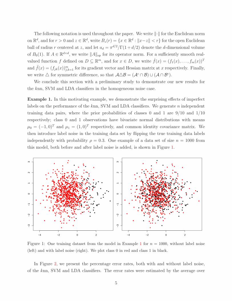
We conclude this section with a preliminary study to demonstrate our new results for

the knn, SVM and LDA classifiers in the homogeneous noise case.

Example 1. In this motivating example, we demonstrate the surprising effects of imperfect

labels on the performance of the knn, SVM and LDA classifiers. We generate n independent

training data pairs, where the prior probabilities of classes 0 and 1 are 9/10 and 1/10

respectively; class 0 and 1 observations have bivariate normal distributions with means

µ0 = (−1, 0)T and µ1 = (1, 0)T respectively, and common identity covariance matrix. We

then introduce label noise in the training data set by flipping the true training data labels

independently with probability ρ = 0.3. One example of a data set of size n = 1000 from

this model, both before and after label noise is added, is shown in Figure 1.

−4 −2 0 2

−3

−2

−1

01

23

−4 −2 0 2

−3

−2

−1

01

23

Figure 1: One training dataset from the model in Example 1 for n = 1000, without label noise

(left) and with label noise (right). We plot class 0 in red and class 1 in black.

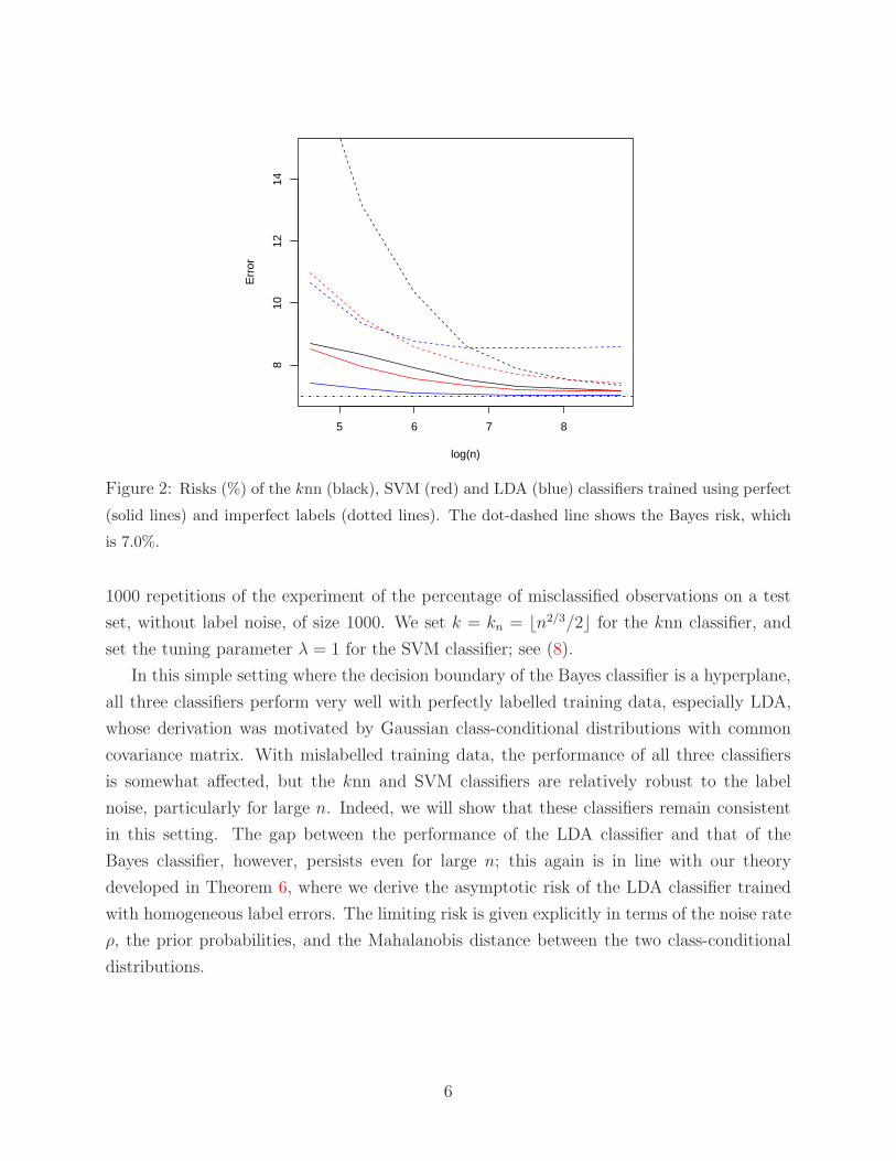
In Figure 2, we present the percentage error rates, both with and without label noise,

of the knn, SVM and LDA classifiers. The error rates were estimated by the average over

5

5 6 7 8

810

1214

log(n)

Err

or

Figure 2: Risks (%) of the knn (black), SVM (red) and LDA (blue) classifiers trained using perfect

(solid lines) and imperfect labels (dotted lines). The dot-dashed line shows the Bayes risk, which

is 7.0%.

1000 repetitions of the experiment of the percentage of misclassified observations on a test

set, without label noise, of size 1000. We set k = kn = ⌊n2/3/2⌋ for the knn classifier, and

set the tuning parameter λ = 1 for the SVM classifier; see (8).

In this simple setting where the decision boundary of the Bayes classifier is a hyperplane,

all three classifiers perform very well with perfectly labelled training data, especially LDA,

whose derivation was motivated by Gaussian class-conditional distributions with common

covariance matrix. With mislabelled training data, the performance of all three classifiers

is somewhat affected, but the knn and SVM classifiers are relatively robust to the label

noise, particularly for large n. Indeed, we will show that these classifiers remain consistent

in this setting. The gap between the performance of the LDA classifier and that of the

Bayes classifier, however, persists even for large n; this again is in line with our theory

developed in Theorem 6, where we derive the asymptotic risk of the LDA classifier trained

with homogeneous label errors. The limiting risk is given explicitly in terms of the noise rate

ρ, the prior probabilities, and the Mahalanobis distance between the two class-conditional

distributions.

6

2 Statistical setting

Let X be a measurable space. In the basic binary classification problem, we observe indepen-

dent and identically distributed training data pairs (X1, Y1), . . . , (Xn, Yn) taking values in

X ×0, 1 with joint distribution P . The task is to predict the class Y of a new observation

X , where (X, Y ) ∼ P is independent of the training data.

Define the prior probabilities π1 = P(Y = 1) = 1 − π0 ∈ (0, 1) and class-conditional

distributions X | Y = r ∼ Pr for r = 0, 1. The marginal feature distribution of X is

denoted PX and we define the regression function η(x) = P(

Y = 1 | X = x). A classifier

C is a measurable function from X to 0, 1, with the interpretation that a point x ∈ X is

assigned to class C(x).

The risk of a classifier C is R(C) = PC(X) 6= Y ; it is minimized by the Bayes classifier

CBayes(x) =

1 if η(x) ≥ 1/2

0 otherwise.

However, since η is typically unknown, in practice we construct a classifier Cn, say, that

depends on the n training data pairs. We say (Cn) is consistent if R(Cn)−R(CBayes) → 0 as

n→ ∞. When we write R(Cn) here, we implicitly assume that Cn is a measurable function

from (X × 0, 1)n × X to 0, 1, and the probability is taken over the joint distribution of

(X1, Y1), . . . , (Xn, Yn), (X, Y ). It is convenient to set S = x ∈ X : η(x) = 1/2.

In this paper, we study settings where the true class labels Y1, . . . , Yn for the training

data are not observed. Instead we see Y1, . . . , Yn, where the noisy label Yi still takes val-

ues in 0, 1, but may not be the same as Yi. The task, however, is still to predict the

true class label Y associated with the test point X . We can therefore consider an aug-

mented model where (X, Y, Y ), (X1, Y1, Y1), . . . , (Xn, Yn, Yn) are independent and identically

distributed triples taking values in X × 0, 1 × 0, 1.

At this point the dependence between Y and Y is left unrestricted, but we introduce the

following notation: define measurable functions ρ0, ρ1 : X → [0, 1] by ρr(x) = P(Y 6= Y |

X = x, Y = r). Thus, letting Z | X = x, Y = r ∼ Bin(1, 1 − ρr(x)) for r = 0, 1, we

can write Y = ZY + (1 − Z)(1 − Y ). We refer to the case where ρ0(x) = ρ1(x) = ρ for all

x ∈ X as ρ-homogeneous noise. Further, let P denote the joint distribution of (X, Y ), and

let η(x) = P(Y = 1 | X = x) denote the regression function for Y , so that

η(x) = η(x)P(Y = 1 | X = x, Y = 1) + 1− η(x)P(Y = 1 | X = x, Y = 0)

= η(x)1− ρ1(x) + 1− η(x)ρ0(x). (1)

7

We also define the corrupted Bayes classifier

CBayes(x) =

1 if η(x) ≥ 1/2

0 otherwise,

which minimizes the corrupted risk R(C) = PC(X) 6= Y .

3 Excess risk bounds for arbitrary classifiers

A key property in this work will be that the Bayes classifier is preserved under label noise;

more specifically, in Theorem 1(i) below, we will provide conditions under which

PX

(

x ∈ Sc : CBayes(x) 6= CBayes(x))

= 0. (2)

In Theorem 1(ii), we go on to show that, under slightly stronger conditions on the label error

probabilities and for an arbitrary classifier C, we can bound the excess risk R(C)−R(CBayes)

of predicting the true label by a multiple of the excess risk of predicting a noisy label

R(C)− R(CBayes), where this multiple does not depend on the classifier C. This latter result

is particularly useful when the classifier C is trained using the imperfect labels, that is with

the training data (X1, Y1), . . . , (Xn, Yn), because, as will be shown in the next section, we

are able to provide further control of R(C)− R(CBayes) for specific choices of C.

It is convenient to let B = x ∈ Sc : ρ0(x) + ρ1(x) < 1, and let

A =

x ∈ B :ρ1(x)− ρ0(x)

2η(x)− 11− ρ0(x)− ρ1(x)< 1

.

Theorem 1. (i) We have

PX

(

Ax ∈ B : CBayes(x) = CBayes(x))

= 0. (3)

In particular, if PX(Ac ∩ Sc) = 0, then (2) holds.

(ii) Now suppose, in fact, that there exist ρ∗ < 1/2 and a∗ < 1 such that PX(x ∈ Sc :

ρ0(x) + ρ1(x) > 2ρ∗) = 0, and

PX

(

x ∈ B :ρ1(x)− ρ0(x)

2η(x)− 11− ρ0(x)− ρ1(x)> a∗

)

= 0.

Then, for any classifier C,

R(C)− R(CBayes) ≤R(C)− R(CBayes)

(1− 2ρ∗)(1− a∗).

8

In Theorem 1(i), the condition PX(Ac ∩ Sc) = 0 restricts the difference between the two

mislabelling probabilities at PX -almost all x ∈ Sc, with stronger restrictions where η(x) is

close to 1/2 and where ρ0(x) + ρ1(x) is close to 1. Moreover, since A ⊆ B, we also have

PX(Bc ∩Sc) = 0, which limits the total amount of label noise at each point; cf. Menon et al.

(2016, Assumption 1). In particular, it ensures that

P(Y 6= Y | X = x) = η(x)ρ1(x) + 1− η(x)ρ0(x) < 1,

for PX-almost all x ∈ Sc. In part (ii), the requirement on a∗ imposes a slightly stronger

restriction on the same weighted difference between the two mislabelling probabilities com-

pared with part (i).

The conditions in Theorem 1 generalize those given in the existing literature by allowing

a wider class of noise mechanisms. For instance, in the case of ρ-homogeneous noise, we

have PX(Ac ∩ Sc) = 0 provided only that ρ < 1/2. In fact, in this setting, we may take

a∗ = 0 (Ghosh et al., 2015, Theorem 1). More generally, we may also take a∗ = 0 if the noise

depends only on the feature vector and not the true class label, i.e. ρ0(x) = ρ1(x) for all x

(Menon et al., 2016, Proposition 4).

The proof of Theorem 1(ii) relies on the following proposition, which provides a bound

on the excess risk for predicting a true label, assuming only that (2) holds.

Proposition 1. Assume that (2) holds. Further, for κ > 0, let

Aκ =

x ∈ X : |2η(x)− 1| ≤ κ|2η(x)− 1|

.

Then, for any classifier C,

R(C)−R(CBayes) ≤ min[

PC(X) 6= CBayes(X), infκ>0

κR(C)−R(CBayes)+PX(Acκ)]

. (4)

Our main focus in this work is on settings where CBayes and CBayes agree, i.e. (2) holds,

because this is where we can hope for classifiers to be robust to label noise. However,

in this instance, we present a more general version of Proposition 1 as Proposition 3 in

the appendix; this bounds the excess risk of an arbitrary classifier without the assumption

that (2) holds. We see in that result, there is an additional contribution to the risk bound

of R(CBayes) − R(CBayes) ≥ 0. See also, for instance, Natarajan et al. (2013), who study

asymmetric homogeneous noise, where ρ0(x) = ρ0 6= ρ1 = ρ1(x), with ρ0 and ρ1 known.

We can regard |2η(x)−1| as a measure of the ease of classifying x. Hence, in Proposition 1,

we can interpret Aκ as the set of points x where the relative difficulty of classifying x in the

corrupted problem compared with its uncorrupted version is controlled. The level of this

control can then be traded off against the measure of the exceptional set Acκ.

9

To provide further understanding of Proposition 1, observe that in general, we have

R(C)− R(CBayes) =

∫

X

[

PC(x) = 0 − 1η(x)<1/2

]

2η(x)− 1 dPX(x)

≤ PC(X) 6= CBayes(X).

Thus, if PX(Ac1) = 0, then the second term in the minimum in (4) gives a better bound

than the first. However, typically in practice, we would have that PX(Ac1) 6= 0, and indeed,

in Example 3 in the appendix, we show that for the 1-nearest neighbour classifier with

homogeneous noise, either of the two terms in the minimum in (4) can be smaller, depending

on the noise level. As a consequence of Proposition 1, we have the following corollary.

Corollary 2. Suppose that (Cn) is a sequence of classifiers satisfying R(Cn) → R(CBayes)

and assume that (2) holds. Further, let S = x ∈ X : η(x) = 1/2. Then

lim supn→∞

R(Cn)− R(CBayes) ≤ PX(S \ S).

In particular, if PX(S \ S) = 0, then R(Cn) → R(CBayes) as n→ ∞.

The condition R(Cn) → R(CBayes) asks that the classifier is consistent for predicting a

corrupted test label. In Section 4 we will see that appropriate versions of the corrupted

knn and SVM classifiers satisfy this condition, provided, in the latter case, that the feature

vectors have compact support. To understand the strength of Corollary 2, consider the

special case of ρ-homogeneous noise, and a classifier Cn that is consistent for predicting a

noisy label when trained with corrupted data. Then S = S by (1), so provided only that

ρ < 1/2, Corollary 2 ensures that Cn remains consistent for predicting a true label when

trained using the corrupted data.

4 Asymptotic properties

4.1 The k-nearest neighbour classifier

We now specialize to the case X = Rd. The knn classifier assigns the test point X to a class

based on a majority vote over the class labels of the k nearest points among the training

data. More precisely, given x ∈ Rd, let (X(1), Y(1)), . . . , (X(n), Y(n)) be the reordering of the

training data pairs such that

‖X(1) − x‖ ≤ . . . ≤ ‖X(n) − x‖,

10

where ties are broken by preserving the original ordering of the indices. For k ∈ 1, . . . , n,

the k-nearest neighbour classifier is

Cknn(x) = Cknnn (x) =

1 if 1k

∑ki=1 1Y(i)=1 ≥ 1/2

0 otherwise.

This simple and intuitive method has received considerable attention since it was intro-

duced by Fix & Hodges (1951, 1989). Stone (1977) showed that the knn classifier is univer-

sally consistent, i.e., R(Cknn) → R(CBayes) for any distribution P , as long as k = kn → ∞

and k/n → 0 as n → ∞. For a substantial overview of the early work on the theoretical

properties of the knn classifier, see Devroye et al. (1996). Further recent studies include

Kulkarni & Posner (1995), Audibert & Tsybakov (2007), Hall et al. (2008), Biau et al.

(2010), Samworth (2012), Chaudhuri & Dasgupta (2014), Gadat et al. (2016), Celisse &

Mary-Huard (2018) and Cannings et al. (2018).

Here we study the properties of the corrupted k-nearest neighbour classifier

Cknn(x) = Cknnn (x) =

1 if 1k

∑ki=1 1Y(i)=1 ≥ 1/2

0 otherwise,

where Y(i) denotes the corrupted label of (X(i), Y(i)). Since the knn classifier is universally

consistent, we have R(Cknn) → R(CBayes) for any choice of k satisfying Stone’s conditions.

Thus, by Corollary 2, if (2) holds and PX(S \ S) = 0, then the corrupted knn classifier

remains universally consistent. In particular, in the special case of ρ-homogeneous noise,

provided only that ρ < 1/2, this result tells us that the corrupted knn classifier remains

universally consistent.

We now show that, under further regularity conditions on the data distribution P and

the noise mechanism, it is possible to give a more precise description of the asymptotic er-

ror properties of the corrupted knn classifier. Since our conditions on P , which are slight

simplifications of those used in Cannings et al. (2018) to analyse the uncorrupted knn clas-

sifier, are a little technical, we give an informal summary of them here, deferring formal

statements of our assumptions A1–A4 to just before the proof of Theorem 3 in Section A.2.

First, we assume that each of the class-conditional distributions has a density with respect

to Lebesgue measure such that the marginal feature density f is continuous and positive.

It turns out that the dominant terms in the asymptotic expansion of the excess risk of knn

classifiers are driven by the behaviour of P in a neighbourhood Sǫ of the set S, which consists

of points that are difficult to classify correctly, so we ask for further regularity conditions on

the restriction of P to Sǫ. In particular, we ask for both f and η to have two well-behaved

derivatives in Sǫ, and for η to be bounded away from 0 on S. This amounts to asking that

11

the class-conditional densities, when weighted by the prior probabilities of each class, cut at

an angle, and ensures that the set S is a (d−1)-dimensional orientable manifold. Away from

the set Sǫ, we only require weaker conditions on PX , and for η to be bounded away from 1/2.

Finally, we ask for two αth moment conditions to hold, namely that∫

Rd ‖x‖α dPX(x) < ∞

and∫

Sf(x0)

d/(α+d) dVold−1(x0) <∞, where dVold−1 denotes the (d− 1)-dimensional volume

form on S.

For β ∈ (0, 1/2), let Kβ = ⌈(n− 1)β⌉, . . . , ⌊(n− 1)1−β⌋ denote the set of values of k to

be considered for the knn classifier. Define

B1 =

∫

S

f(x0)

4‖η(x0)‖dVold−1(x0), B2 =

∫

S

f(x0)1−4/d

‖η(x0)‖a(x0)

2 dVold−1(x0),

where

a(x) =

∑dj=1

ηj(x)fj(x) +12ηjj(x)f(x)

(d+ 2)a2/dd f(x)

.

We will also make use of a condition on the noise rates near the Bayes decision boundary:

Assumption B1. There exist δ > 0 and a function g : (1/2 − δ, 1/2 + δ) → [0, 1) that is

differentiable at 1/2, with the property that for x such that η(x) ∈ (1/2− δ, 1/2 + δ),

we have ρ0(x) = g(η(x)) and ρ1(x) = g(1− η(x)).

This assumption asks that, when η(x) is close to 1/2, the probability of label noise depends

only on x through η(x), and moreover, this probability varies smoothly with η(x). In other

words, Assumption B1 says that the probability of mislabelling an observation with true

class label 0 depends only on the extent to which it appeared to be from class 1; conversely,

the probability of mislabelling an observation with true label 1 depends only, and in a

symmetric way, on the extent to which it appeared to be from class 0. To give just one of

many possible examples, one could imagine that the probability that a doctor misdiagnoses

a malignant tumour as benign depends on the extent to which it appears to be malignant,

and vice versa. We remark that Menon et al. (2016, Definition 11) introduce a related

probabilistically transformed noise model, where ρ0 = g0 η and ρ1 = g1 η, but they also

require that g0 and g1 are increasing on [0, 1/2] and decreasing on [1/2, 1]; see also Bylander

(1997).

Theorem 3. Assume A1, A2, A3 and A4(α). Suppose that ρ0, ρ1 are continuous, and that

both

ρ∗ =1

2supx∈Rd

ρ0(x) + ρ1(x) <1

2

and

a∗ = supx∈B

ρ1(x)− ρ0(x)

2η(x)− 11− ρ0(x)− ρ1(x)< 1.

12

Moreover, assume B1 holds with the additional requirement that g is twice continuously

differentiable, g(1/2) > 2g(1/2)− 1 and that g is uniformly continuous. Then we have two

cases:

(i) Suppose that d ≥ 5 and α > 4d/(d− 4). Then for each β ∈ (0, 1/2),

R(Cknn)− R(CBayes) =B1

k1− 2g(1/2) + g(1/2)2+B2

(k

n

)4/d

+ o

(

1

k+(k

n

)4/d)

as n→ ∞, uniformly for k ∈ Kβ.

(ii) Suppose that either d ≤ 4, or, d ≥ 5 and α ≤ 4d/(d− 4). Then for each β ∈ (0, 1/2)

and each ǫ > 0 we have

R(Cknn)−R(CBayes) =B1

k1− 2g(1/2) + g(1/2)2+ o

(1

k+(k

n

)α

α+d−ǫ)

as n→ ∞, uniformly for k ∈ Kβ.

The proof of Theorem 3 is given in Section A.2, and involves two key ideas. First,

we demonstrate that the conditions assumed for η also hold for the corrupted regression

function η. Second, we show that the dominant asymptotic contribution to the desired

excess risk R(Cknn)− R(CBayes) is R(Cknn)− R(CBayes)/1− 2g(1/2) + g(1/2), a scalar

multiple of the excess risk when predicting a noisy label. We then conclude the argument by

appealing to Cannings et al. (2018, Theorem 1), and of course, can recover the conclusion

of that result for noiseless labels as a special case of Theorem 3 by setting g = 0.

In the conclusion of Theorem 3(i), the terms B1/[k1−2g(1/2)+g(1/2)2] and B2(k/n)4/d

can be thought of as the leading order contributions to the variance and squared bias of the

corrupted knn classifier respectively. It is both surprising and interesting to note that the

type of label noise considered here affects only the leading order variance term compared

with the noiseless case; the dominant bias term is unchanged. To give a concrete example, ρ-

homogeneous noise satisfies the conditions of Theorem 3, and in the setting of Theorem 3(i),

we see that the dominant variance term is inflated by a factor of (1− 2ρ)−2.

We now quantify the relative asymptotic performance of the corrupted knn and uncor-

rupted knn classifiers. Since this performance depends on the choice of k in each case, we

couple these choices together in the following way: given any k to be used by the uncorrupted

classifier Cknn, and given the function g from Theorem 3, we consider the choice

kg =⌊

1− 2g(1/2) + g(1/2)−2d/(d+4)k⌋

(5)

for the noisy label classifier Cknn. This coupling reflects the ratio of the optimal choices of k

for the corrupted and uncorrupted label settings.

13

Corollary 4. Under the assumptions of Theorem 3(i), and provided that B2 > 0, we have

that for any β ∈ (0, 1/2),

R(Ckgnn)− R(CBayes)

R(Cknn)− R(CBayes)→ 1− 2g(1/2) + g(1/2)−8/(d+4), (6)

as n→ ∞, uniformly for k ∈ Kβ.

If g(1/2) > 2g(1/2), then the limiting regret ratio in (6) is less than 1 – this means that

the label noise helps in terms of the asymptotic performance! This is due to the fact that,

under the noise model in Theorem 3, if g(1/2) > 2g(1/2) then for points Xi with η(Xi) close

to 1/2, the noisy labels Yi are more likely than the true labels Yi to be equal to the Bayes

labels, 1η(Xi)≥1/2. To understand this phenomenon, first note that by rearranging (1), we

have

η(x)− 1/2 = η(x)− 1/21− ρ0(x)− ρ1(x)+1

2ρ0(x)− ρ1(x).

Thus η(x)− 1/2 = η(x)− 1/2 for x ∈ S using B1. On the other hand, for x ∈ Sc, we have

η(x)− 1/2 = η(x)− 1/2

(

1− ρ0(x)− ρ1(x) +ρ0(x)− ρ1(x)

2η(x)− 1

)

. (7)

We next study the term in the second parentheses on the right-hand side above. Write

t = η(x)− 1/2. Then, for x such that |η(x)− 1/2| ∈ (0, δ), we have ρ0(x) = g(1/2 + t) and

ρ1(x) = g(1/2− t). It follows, for such x, that

1−ρ0(x)−ρ1(x)+ρ0(x)− ρ1(x)

2η(x)− 1= 1− g(1/2 + t)− g(1/2− t) +

g(1/2 + t)− g(1/2− t)

2t

→ 1− 2g(1/2) + g(1/2)

as |t| ց 0. Since 1−2g(1/2)+ g(1/2) > 1, we obtain that for any ε ∈(

0, g(1/2)/2−g(1/2))

,

there exists δ0 ∈ (0, δ) such that for all x with |η(x)− 1/2| ∈ (0, δ0), we have that

1− ρ0(x)− ρ1(x) +ρ0(x)− ρ1(x)

2(η(x)− 1/2)> 1− 2g(1/2) + g(1/2)− ε > 1.

This together with (7) ensures that, for all x such that |η(x)− 1/2| ∈ (0, δ0), we have

|η(x)− 1/2| > |η(x)− 1/2|.

Example 2. Suppose that for some g0 ∈ (0, 1/2) and h0 > 2 − 1/g0 we have g(1/2 + t) =

g0(1 + h0t) for t ∈ (−δ, δ). Then g(1/2) = g0 and g(1/2) = g0h0, which gives 1 − 2g(1/2) +

g′(1/2) = 1+ (h0 − 2)g0. We therefore see from Corollary 4 that if h0 < 2, then the limiting

regret ratio is greater than 1, but if h0 > 2, then the limiting regret ratio is less than one,

so the label noise aids performance.

14

4.2 Support vector machine classifiers

In general, the term support vector machines (SVM) refers to classifiers of the form

CSVM(x) = CSVMn (x) =

1 if f(x) ≥ 0

0 otherwise,

where the decision function f satisfies

f ∈ argminf∈H

1

n

n∑

i=1

L(Yi, f(Xi)) + Ω(λ, ‖f‖H)

.

See, for example, Cortes & Vapnik (1995) and Steinwart & Christmann (2008). Here L :

R× R → R is a loss function, Ω : R× R → R is a regularization function, λ > 0 is a tuning

parameter and H is a reproducing kernel Hilbert space (RKHS) with norm ‖ · ‖H (Steinwart

& Christmann, 2008, Chapter 4).

We focus throughout on the L1-SVM, where L(y, t) = max0, 1− (2y− 1)t is the hinge

loss function and Ω(λ, t) = λt2. Let K : Rd × R

d → R be the positive definite kernel

function associated with the RKHS. We consider the Gaussian radial basis function, namely

K(x, x′) = exp(−σ2‖x− x′‖2), for σ > 0. The corrupted SVM classifier is

CSVM(x) = CSVMn (x) =

1 if f(x) ≥ 0

0 otherwise,(8)

where

f ∈ argminf∈H

1

n

n∑

i=1

max0, 1− (2Yi − 1)f(Xi)+ λ‖f‖2H

. (9)

Steinwart (2005, Corollary 3.6 and Example 3.8) show that the uncorrupted L1-SVM

classifier is consistent as long as PX is compactly supported and λ = λn is such that λn → 0

but nλn/(| logλn|d+1) → ∞. Therefore, under these conditions, provided that (2) holds and

PX(S \ S) = 0, by Corollary 2, we have that R(CSVM) → R(CBayes) as n→ ∞.

Under further conditions on the noise probabilities and the distribution P , we can also

provide more precise control of the excess risk for the SVM classifier. Our analysis will make

use of the results in Steinwart & Scovel (2007), who study the rate of convergence of the

SVM classifier with Gaussian kernels in the noiseless label setting. Other works of note on

the rate of convergence of SVM classifiers include Lin (1999) and Blanchard et al. (2008);

see also Steinwart & Christmann (2008, Chapters 6 and 8).

We recall two definitions used in the perfect labels context. The first of these is the

well-known margin assumption of, for example, Audibert & Tsybakov (2007). We say that

15

the distribution P satisfies the margin assumption with parameter γ1 ∈ [0,∞) if there exists

κ1 > 0 such that

PX(x ∈ Rd : 0 < |η(x)− 1/2| ≤ t) ≤ κ1t

γ1

for all t > 0. If P satisfies the margin assumption for all γ1 ∈ [0,∞) then we say P satisfies

the margin assumption with parameter ∞. The margin assumption controls the probability

mass of the region where η is close to 1/2.

The second definition we need is that of the geometric noise exponent (Steinwart & Scovel,

2007, Definition 2.3). Let S+ = x ∈ Rd : η(x) > 1/2 and S− = x ∈ R

d : η(x) < 1/2, and

for x ∈ Rd, let τx = infx′∈S∪S+ ‖x − x′‖ + infx′∈S∪S−

‖x − x′‖. We say that the distribution

P has geometric noise exponent γ2 ∈ [0,∞) if there exists κ2 > 0, such that∫

Rd

|2η(x)− 1| exp(

−τ 2xt2

)

dPX(x) ≤ κ2tγ2d

for all t > 0. If P has geometric noise exponent γ2 for all γ2 ∈ [0,∞) then we say it has

geometric noise exponent ∞.

Under these two conditions, Steinwart & Scovel (2007, Theorem 2.8) show that, if PX is

supported on the closed unit ball, then for appropriate choices of the tuning parameters, the

SVM classifier achieves a convergence rate of O(n−Γ+ǫ) for every ǫ > 0, where

Γ =

γ22γ2+1

if γ2 ≤γ1+22γ1

2γ2(γ1+1)2γ2(γ1+2)+3γ1+4

otherwise.

In the imperfect labels setting, and under our stronger assumption on the noise mech-

anism when η is close to 1/2, we see that the SVM classifier trained with imperfect labels

satisfies the same bound on the rate of convergence as in the perfect labels case.

Theorem 5. Suppose that P satisfies the margin assumption with parameter γ1 ∈ [0,∞],

has geometric noise exponent γ2 ∈ (0,∞) and that PX is supported on the closed unit ball.

Assume the conditions of Theorem 1(ii) and B1 holds. Then

R(CSVM)− R(CBayes) = O(n−Γ+ǫ),

as n→ ∞, for every ǫ > 0. If γ2 = ∞, then the same conclusion holds provided σn = σ is a

constant with σ > 2d1/2.

4.3 Linear discriminant analysis

If P0 = Nd(µ0,Σ) and P1 = Nd(µ1,Σ), then the Bayes classifier is

CBayes(x) =

1 if log(

π1

π0

)

+(

x− µ1+µ0

2

)TΣ−1(µ1 − µ0) ≥ 0

0 otherwise.(10)

16

The Bayes risk can be expressed in terms of π0, π1, and the squared Mahalanobis distance

∆2 = (µ1 − µ0)TΣ−1(µ1 − µ0) between the classes as

R(CBayes) = π0Φ

(

1

∆log

(π1π0

)

−∆

2

)

+ π1Φ

(

1

∆log

(π0π1

)

−∆

2

)

,

where Φ denotes the standard normal distribution function.

The LDA classifier is constructed by substituting training data estimates of π0, π1, µ0, µ1,

and Σ in to (10). With imperfect training data labels, and for r = 0, 1, we define estimates

πr = n−1∑n

i=1 1Yi=r of πr, as well as estimates µr =∑n

i=1Xi1Yi=r/∑n

i=1 1Yi=r of the

class-conditional means µr, and set

Σ =1

n− 2

n∑

i=1

1∑

r=0

(Xi − µr)(Xi − µr)T1Yi=r.

This allows us to define the corrupted LDA classifier

CLDA(x) = CLDAn (x) =

1 if log(

π1

π0

)

+(

x− µ1+µ0

2

)TΣ−1(µ1 − µ0) ≥ 0

0 otherwise.

Consider now the ρ-homogeneous noise setting. In this case, writing Pr, r ∈ 0, 1, for

the distribution of X | Y = r, we have Pr = prNd(µr,Σ) + (1 − pr)Nd(µ1−r,Σ), where

pr = πr(1 − ρ)/πr(1 − ρ) + π1−rρ. Notice that while πr, µr and Σ are intended to be

estimators of πr, µr and Σ, respectively, with label noise these will in fact be consistent

estimators of πr = πr(1−ρ)+π1−rρ, µr = prµr+(1−pr)µ1−r, and Σ = Σ+α(µ1−µ0)(µ1−µ0)T ,

respectively, where α > 0 is given in the proof of Theorem 6.

We will also make use of the following well-known lemma in the homogeneous label noise

case (e.g. Ghosh et al., 2015, Theorem 1), which holds for an arbitrary classifier and data

generating distribution. We include the short proof for completeness.

Lemma 2. For ρ-homogeneous noise with ρ ∈ [0, 1/2) and for any classifier C, we have

R(C) = R(C)−ρ/(1−2ρ). Moreover, R(C)−R(CBayes) =

R(C)− R(CBayes)

/(1−2ρ).

The following is the main result of this subsection.

Theorem 6. Suppose that Pr = Nd(µr,Σ) for r = 0, 1 and that the noise is ρ-homogeneous

with ρ ∈ [0, 1/2). Then

limn→∞

CLDA(x) =

1 if c0 +(

x− µ1+µ0

2

)TΣ−1(µ1 − µ0) > 0

0 if c0 +(

x− µ1+µ0

2

)TΣ−1(µ1 − µ0) < 0,

17

where

c0=

(1− 2ρ) +ρ(1−ρ)(1+π0π1∆

2)

(1− 2ρ)π1π0

log((1− 2ρ)π1 + ρ

(1− 2ρ)π0 + ρ

)

−(π1 − π0)ρ(1− ρ)∆2

2(1−2ρ)2π1π0 + ρ(1−ρ).

As a consequence,

limn→∞

R(CLDA) = π0Φ

(

c0∆

−∆

2

)

+ π1Φ

(

−c0∆

−∆

2

)

≥ R(CBayes). (11)

For each ρ ∈ (0, 1/2) and π0 6= π1, there exists a unique value of ∆ > 0 for which equality

in the inequality in (11) is attained.

The first conclusion of this theorem reveals the interesting fact that, regardless of the level

ρ ∈ (0, 1/2) of label noise, the limiting corrupted LDA classifier has a decision hyperplane

that is parallel to that of the Bayes classifier; see also Lachenbruch (1966) and Manwani

& Sastry (2013, Corollary 1). However, for each fixed ρ ∈ (0, 1/2) and π0 6= π1, there is

only one value of ∆ > 0 for which the offset is correct and the corrupted LDA classifier is

consistent.

5 Numerical comparison

In this section, we investigate empirically how the different types of label noise affect the

performance of the k-nearest neighbour, support vector machine and linear discriminant

analysis classifiers. We consider two different model settings for the pair (X, Y ):

Model 1: Let P(Y = 1) = π1 ∈ 0.5, 0.9 and X | Y = r ∼ Nd(µr, Id), where

µ1 = (3/2, 0, . . . , 0)T = −µ0 ∈ Rd and Id denotes the d by d identity matrix.

Model 2: For d ≥ 2, let X ∼ U([0, 1]d) and P(Y = 1 | X = x) = η(x1, . . . , xd) =

min4(x1 − 1/2)2 + 4(x2 − 1/2)2, 1.

In each setting, our risk estimates are based on an uncorrupted test set of size 1000, and

we repeat each experiment 1000 times. This ensures that all standard errors are less than

0.4% and 0.14 for the risk and regret ratio estimates, respectively; in fact, they are often

much smaller.

Our first goal is to illustrate numerically our consistency and inconsistency results for

the knn, SVM and LDA classifiers. In Figure 3 we present estimates of the risk for the three

classifiers with different levels of homogeneous label noise. We see that for Model 1 when

the class prior probabilities are equal, all three classifiers perform well and in particular

appear to be consistent, even when as many as 30% of the training data labels are incorrect

on average. For the knn and SVM classifiers we observe very similar results for Model 2;

18

4 5 6 7 8

810

1214

1618

log(n)

Err

or

4 5 6 7 8

1015

2025

log(n)

Err

or

4 5 6 7 8

810

1214

16

log(n)

Err

or

4 5 6 7 8

2025

3035

40

log(n)

Err

or

4 5 6 7 8

2025

3035

40

log(n)

Err

or

4 5 6 7 8

2025

3035

4045

5055

log(n)

Err

or

Figure 3: Risk estimates for the knn (left), SVM (middle) and LDA (right) classifiers. Top:

Model 1, d = 2, π1 = 0.5, Bayes risk = 6.68%, shown as the black dotted line. Bottom: Model 2, d =

2, Bayes risk = 19.63%. We present the results without label noise (black) and with homogeneous

label noise at rate ρ = 0.1 (red) and 0.3 (blue).

the LDA classifier does not perform well in this setting, however, since the Bayes decision

boundary is non-linear. These conclusions are in accordance with Corollary 2 and Theorem 6.

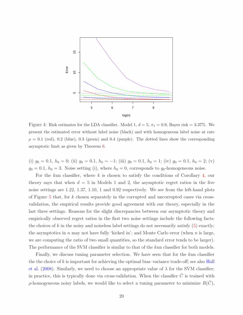
We further investigate the effect of homogeneous label noise on the performance of the

LDA classifier for data from Model 1, but now when d = 5 and the class prior probabilities

are unbalanced. Recall that in Theorem 6 we derived the asymptotic limit of the risk in terms

of the Mahalanobis distance between the true class distributions, the class prior probabilities

and the noise rate. In Figure 4, we present the estimated risks of the LDA classifier for data

from Model 1 with π1 = 0.9 for different homogeneous noise rates alongside the limit as

specified by Theorem 6. This articulates the inconsistency of the corrupted LDA classifier,

as observed in Theorem 6.

Finally, we study empirically the asymptotic regret ratios for the knn and SVM classifiers.

We focus on the noise model in Example 2 in Section 4, where the label errors occur at random

as follows: fix g0 ∈ (0, 1/2), h0 > 2− 1/g0, we let g(1/2+ t) = max[0,ming0(1+ h0t), 2g0],

then set ρ0(x) = g(η(x)) and ρ1(x) = g(1−η(x)). In particular, we use the following settings:

19

5 6 7 8

510

15

log(n)

Err

or

Figure 4: Risk estimates for the LDA classifier. Model 1, d = 5, π1 = 0.9, Bayes risk = 3.37%. We

present the estimated error without label noise (black) and with homogeneous label noise at rate

ρ = 0.1 (red), 0.2 (blue), 0.3 (green) and 0.4 (purple). The dotted lines show the corresponding

asymptotic limit as given by Theorem 6.

(i) g0 = 0.1, h0 = 0; (ii) g0 = 0.1, h0 = −1; (iii) g0 = 0.1, h0 = 1; (iv) g0 = 0.1, h0 = 2; (v)

g0 = 0.1, h0 = 3. Noise setting (i), where h0 = 0, corresponds to g0-homogeneous noise.

For the knn classifier, where k is chosen to satisfy the conditions of Corollary 4, our

theory says that when d = 5 in Models 1 and 2, the asymptotic regret ratios in the five

noise settings are 1.22, 1.37, 1.10, 1 and 0.92 respectively. We see from the left-hand plots

of Figure 5 that, for k chosen separately in the corrupted and uncorrupted cases via cross-

validation, the empirical results provide good agreement with our theory, especially in the

last three settings. Reasons for the slight discrepancies between our asymptotic theory and

empirically observed regret ratios in the first two noise settings include the following facts:

the choices of k in the noisy and noiseless label settings do not necessarily satisfy (5) exactly;

the asymptotics in n may not have fully ‘kicked in’; and Monte Carlo error (when n is large,

we are computing the ratio of two small quantities, so the standard error tends to be larger).

The performance of the SVM classifier is similar to that of the knn classifier for both models.

Finally, we discuss tuning parameter selection. We have seen that for the knn classifier

the the choice of k is important for achieving the optimal bias–variance trade-off; see also Hall

et al. (2008). Similarly, we need to choose an appropriate value of λ for the SVM classifier;

in practice, this is typically done via cross-validation. When the classifier C is trained with

ρ-homogeneous noisy labels, we would like to select a tuning parameter to minimize R(C),

20

4.0 4.5 5.0 5.5 6.0 6.5 7.0 7.5

1.0

1.5

2.0

2.5

log(n)

Reg

ret r

atio

4.0 4.5 5.0 5.5 6.0 6.5 7.0 7.5

1.0

1.5

2.0

2.5

log(n)

Reg

ret r

atio

4.0 4.5 5.0 5.5 6.0 6.5 7.0 7.5

1.0

1.2

1.4

1.6

1.8

2.0

log(n)

Reg

ret r

atio

4.0 4.5 5.0 5.5 6.0 6.5 7.0 7.5

1.0

1.2

1.4

1.6

1.8

2.0

log(n)

Reg

ret r

atio

Figure 5: Estimated regret ratios for the knn (left) and SVM (right) classifiers. Top: Model 1,

with d = 5 and π1 = 0.5. Bottom: Model 2, with d = 5. We present the results with label noise of

type (i – red), (ii – blue), (iii – green), (iv – black), and (v – purple).

but since the training data is corrupted, a tuning parameter selection method will target

the minimizer of R(C). However, by Lemma 2, we have that R(C) = R(C)− ρ/(1− 2ρ),

and it follows that our tuning parameter selection method requires no modification when

trained with noisy labels. In the heterogeneous noise case, however, we do not have this

direct relationship; see Inouye et al. (2017) for more on this topic.

In our simulations, we chose k for the knn classifier and λ for the SVM classifier via leave-

one-out and 10-fold cross-validation respectively, where the cross-validation was performed

over the noisy training dataset. Moreover, for the SVM classifier, we used the default choice

σ2 = 1/d for the hyper-parameter for the kernel function.

21

A Proofs and an illustrative example

A.1 Proofs from Section 3

Proof of Theorem 1. (i) First, we have that for PX-almost all x ∈ B,

η(x)− 1/2 = η(x)− 1/21− ρ0(x)− ρ1(x)+1

2ρ0(x)− ρ1(x)

= η(x)− 1/21− ρ0(x)− ρ1(x)

(

1−ρ1(x)− ρ0(x)

2η(x)− 11− ρ0(x)− ρ1(x)

)

.

(12)

Thus, for PX-almost all x ∈ B, we have ρ1(x)−ρ0(x)/[2η(x)−11−ρ0(x)−ρ1(x)] < 1

if and only if

sgnη(x)− 1/2 = sgnη(x)− 1/2.

This completes the proof of (3). It follows that, if PX(Ac ∩ Sc) = 0, then PX(x ∈ B :

CBayes(x) = CBayes(x)c∩Sc) = 0. In other words PX(x ∈ Sc : CBayes(x) 6= CBayes(x)) = 0,

i.e. (2) holds. Here we have used the fact that A ⊆ B, so if PX(Ac ∩ Sc) = 0, then

PX(Bc ∩ Sc) = 0.

(ii) For the proof of this part, we apply Proposition 1. First, since (2) holds, we have

R(CBayes) = R(CBayes). From (12), we have that for PX -almost all x ∈ B,

|2η(x)− 1| = |2η(x)− 1|1− ρ0(x)− ρ1(x)(

1−ρ1(x)− ρ0(x)

2η(x)− 11− ρ0(x)− ρ1(x)

)

≥ |2η(x)− 1|(1− 2ρ∗)(1− a∗). (13)

In fact, the conclusion of (13) remains true (trivially) when x ∈ S. Thus, by Proposition 1,

R(C)− R(CBayes) ≤ infκ>0

κR(C)− R(CBayes)+ PX(Acκ)

≤R(C)− R(CBayes)

(1− 2ρ∗)(1− a∗)+ PX(A

c(1−2ρ∗)−1(1−a∗)−1) =

R(C)− R(CBayes)

(1− 2ρ∗)(1− a∗),

since PX(Ac(1−2ρ∗)−1(1−a∗)−1) ≤ PX(A

c(1−2ρ∗)−1(1−a∗)−1 ∩ B) + PX(B

c) = 0, by (13).

Proposition 1 is a special case of the following result.

Proposition 3. Let D =

x ∈ Sc : CBayes(x) = CBayes(x)

, and recall the definition of Aκ

in Proposition 1. Then, for any classifier C,

R(C)− R(CBayes) ≤ R(CBayes)− R(CBayes) + min[

P

C(X) 6= CBayes(X) ∩ X ∈ D

,

infκ>0

κR(C)− R(CBayes)+ E(

|2η(X)− 1|1X∈D\Aκ

)

]

.

22

Remark: If (2) holds, i.e. PX(Dc ∩ Sc) = 0, then R(CBayes) = R(CBayes), and moreover

we have that E(

|2η(X)− 1|1X∈D\Aκ

)

≤ PX

(

D \ Aκ

)

≤ PX

(

Acκ

)

.

Proof of Proposition 3. First write

R(C) =

∫

X

PC(x) 6= Y | X = x dPX(x)

=

∫

X

[

PC(x) = 0P(Y = 1 | X = x) + PC(x) = 1P(Y = 0 | X = x)]

dPX(x)

=

∫

X

[

PC(x) = 02η(x)− 1+ 1− η(x)]

dPX(x). (14)

Here we have implicitly assumed that the classifier C is random since it may depend on

random training data. However, in the case that C is non-random, one should interpret

PC(x) = 0 as being equal to 1C(x)=0, for x ∈ X .

Now, for PX-almost all x ∈ D,[

PC(x) = 0 − 1η(x)<1/2

]

2η(x)− 1 =∣

∣PC(x) = 0 − 1η(x)<1/2

∣

∣|2η(x)− 1|

≤∣

∣PC(x) = 0 − 1η(x)<1/2

∣

∣

= PC(x) 6= CBayes(x).

Moreover, for PX-almost all x ∈ Dc, we have[

PC(x) = 0 − 1η(x)<1/2

]

2η(x)− 1 ≤ 0 (15)

It follows that

R(C)− R(CBayes) =

∫

X

[

PC(x) = 0 − 1η(x)<1/2

]

2η(x)− 1 dPX(x)

=

∫

D

[

PC(x) = 0 − 1η(x)<1/2

]

2η(x)− 1 dPX(x)

+

∫

Dc

[

PC(x) = 0 − 1η(x)<1/2

]

2η(x)− 1 dPX(x)

≤ P(

C(X) 6= CBayes(X) ∩ X ∈ D)

.

To see the right-hand bound, observe that by (15), for κ > 0,

R(C)− R(CBayes) =

∫

X

[

PC(x) = 0 − 1η(x)<1/2

]

2η(x)− 1 dPX(x)

≤

∫

D

[

PC(x) = 0 − 1η(x)<1/2

]

2η(x)− 1 dPX(x)

≤ κ

∫

D∩Aκ

[

PC(x) = 0 − 1η(x)<1/2

]

2η(x)− 1 dPX(x)

+ E(

|2η(X)− 1|1X∈D\Aκ

)

= κR(C)− R(CBayes)+ E(

|2η(X)− 1|1X∈D\Aκ

)

,

23

where the last step follows from (14).

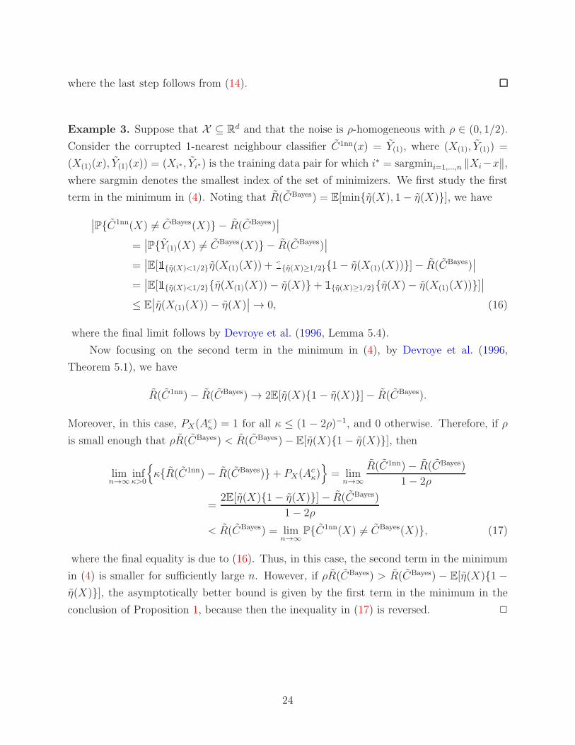
Example 3. Suppose that X ⊆ Rd and that the noise is ρ-homogeneous with ρ ∈ (0, 1/2).

Consider the corrupted 1-nearest neighbour classifier C1nn(x) = Y(1), where (X(1), Y(1)) =

(X(1)(x), Y(1)(x)) = (Xi∗ , Yi∗) is the training data pair for which i∗ = sargmini=1,...,n ‖Xi−x‖,

where sargmin denotes the smallest index of the set of minimizers. We first study the first

term in the minimum in (4). Noting that R(CBayes) = E[minη(X), 1− η(X)], we have

∣

∣PC1nn(X) 6= CBayes(X) − R(CBayes)∣

∣

=∣

∣PY(1)(X) 6= CBayes(X) − R(CBayes)∣

∣

=∣

∣E[1η(X)<1/2η(X(1)(X)) + 1η(X)≥1/21− η(X(1)(X))]− R(CBayes)∣

∣

=∣

∣E[1η(X)<1/2η(X(1)(X))− η(X)+ 1η(X)≥1/2η(X)− η(X(1)(X))]∣

∣

≤ E∣

∣η(X(1)(X))− η(X)∣

∣ → 0, (16)

where the final limit follows by Devroye et al. (1996, Lemma 5.4).

Now focusing on the second term in the minimum in (4), by Devroye et al. (1996,

Theorem 5.1), we have

R(C1nn)− R(CBayes) → 2E[η(X)1− η(X)]− R(CBayes).

Moreover, in this case, PX(Acκ) = 1 for all κ ≤ (1 − 2ρ)−1, and 0 otherwise. Therefore, if ρ

is small enough that ρR(CBayes) < R(CBayes)− E[η(X)1− η(X)], then

limn→∞

infκ>0

κR(C1nn)− R(CBayes)+ PX(Acκ)

= limn→∞

R(C1nn)− R(CBayes)

1− 2ρ

=2E[η(X)1− η(X)]− R(CBayes)

1− 2ρ

< R(CBayes) = limn→∞

PC1nn(X) 6= CBayes(X), (17)

where the final equality is due to (16). Thus, in this case, the second term in the minimum

in (4) is smaller for sufficiently large n. However, if ρR(CBayes) > R(CBayes) − E[η(X)1 −

η(X)], the asymptotically better bound is given by the first term in the minimum in the

conclusion of Proposition 1, because then the inequality in (17) is reversed.

24

Proof of Corollary 2. Let ǫn = max[

supm≥nR(Cm)− R(CBayes)1/2, n−1]

. Then, by Propo-

sition 3,

R(Cn)− R(CBayes) ≤1

ǫnR(Cn)− R(CBayes)+ E

(

|2η(X)− 1|1X∈D\Aǫ−1n

)

≤ R(Cn)− R(CBayes)1/2 + PX(D \ Aǫ−1n

)

.

Since (ǫn) is decreasing, it follows that

lim supn→∞

R(Cn)− R(CBayes) ≤ R(CBayes)− R(CBayes) + PX(S ∩ D).

In particular, if (2) holds, then

lim supn→∞

R(Cn)− R(CBayes) ≤ PX(S \ S),

as required.

A.2 Conditions and proof of Theorem 3

A formal description of the conditions of Theorem 3 is given below:

Assumption A1. The probability measures P0 and P1 are absolutely continuous with re-

spect to Lebesgue measure, with Radon–Nikodym derivatives f0 and f1, respectively.

Moreover, the marginal density of X , given by f = π0f0 + π1f1, is continuous and

positive.

Assumption A2. The set S is non-empty and f is bounded on S. There exists ǫ0 > 0 such

that f is twice continuously differentiable on Sǫ0 = S +Bǫ0(0), and

F (δ) = supx0∈S:f(x0)≥δ

max

‖ ˙f(x0)‖

f(x0),supu∈Bǫ0 (0)

‖ ¨f(x0 + u)‖op

f(x0)

= o(δ−τ) (18)

as δ ց 0, for every τ > 0. Furthermore, recalling ad = πd/2/Γ(1 + d/2) and writing

pǫ(x) = PX(Bǫ(x)), there exists µ0 ∈ (0, ad) such that for all x ∈ Rd and ǫ ∈ (0, ǫ0], we

have

pǫ(x) ≥ µ0ǫdf(x).

Assumption A3. We have infx0∈S ‖η(x0)‖ > 0, so that S is a (d− 1)-dimensional, orientable

manifold. Moreover, supx∈S2ǫ0 ‖η(x)‖ <∞ and η is uniformly continuous on S2ǫ0 with

supx∈S2ǫ0 ‖η(x)‖op <∞. Finally, the function η is continuous, and

infx∈Rd\Sǫ0

|η(x)− 1/2| > 0.

25

Assumption A4(α). We have that∫

Rd ‖x‖α dPX(x) < ∞ and

∫

Sf(x0)

d/(α+d) dVold−1(x0) <

∞, where dVold−1 denotes the (d− 1)-dimensional volume form on S.

Proof of Theorem 3. Part 1: We show that the distribution P of the pair (X, Y ) satisfies

suitably modified versions of Assumptions A1, A2, A3 and A4(α).

Assumption A1: For r ∈ 0, 1, let Pr denote the conditional distribution of X given

Y = r. For x ∈ Rd, and r = 0, 1, define

fr(x) =πr1− ρr(x)fr(x) + π1−rρ1−r(x)f1−r(x)

∫

Rd πr1− ρr(z)f1−r(z) + π1−rρ1−r(z)f1−r(z) dz.

Now, for a Borel subset A of Rd, we have that

P1(A) = P(X ∈ A | Y = 1) =P(X ∈ A, Y = 1)

P(Y = 1)

=π1P(X ∈ A, Y = 1 | Y = 1) + π0P(X ∈ A, Y = 1 | Y = 1)

P(Y = 1)

=π1

∫

A1− ρ1(x)f1(x) dx+ π0

∫

Aρ0(x)f0(x) dx

P(Y = 1)=

∫

A

f1(x) dx.

Similarly, P0(A) =∫

Af0(x) dx. Hence P0 and P1 are absolutely continuous with respect to

Lebesgue measure, with Radon–Nikodym derivatives f0 and f1, respectively. Furthermore,

f = P(Y = 0)f0 + P(Y = 1)f1 = f is continuous and positive.

Assumption A2: Since A2 refers mainly to the marginal distribution of X , which is

unchanged under the addition of label noise, this assumption is trivially satisfied for f = f ,

as long as S = x ∈ Rd : η(x) = 1/2 = S. To see this, let δ0 > 0 and note that for x

satisfying η(x)− 1/2 > δ0, we have from (1) that

η(x)− 1/2 = η(x)− 1/21− ρ0(x)− ρ1(x)

1 +ρ0(x)− ρ1(x)

2η(x)− 11− ρ0(x)− ρ1(x)

> η(x)− 1/2(1− 2ρ∗)(1− a∗) ≥ δ0(1− 2ρ∗)(1− a∗). (19)

Similarly, if 1/2− η(x) > δ0, then we have that 1/2− η(x) > δ0(1− 2ρ∗)(1− a∗). It follows

that S ⊆ S. Now, for x such that |η(x)− 1/2| < δ, we have

η(x)− 1/2 = η(x)− 1/2 + 1− η(x)g(η(x))− η(x)g(1− η(x)). (20)

Thus S ⊆ S.

Assumption A3: Since g is twice continuously differentiable, we have that η is twice

continuously differentiable on the set x ∈ S2ǫ0 : |η(x)− 1/2| < δ. On this set, its gradient

vector at x is

˙η(x) = η(x)[

1− g(η(x))− g(1− η(x)) + 1− η(x)g(η(x)) + η(x)g(1− η(x))]

.

26

The corresponding Hessian matrix at x is

¨η(x) = η(x)[

1− g(η(x))− g(1− η(x)) + 1− η(x)g(η(x)) + η(x)g(1− η(x))]

− η(x)[

η(x)T g(η(x))− η(x)T g(1− η(x)) + η(x)T g(η(x))

− 1− η(x)η(x)T g(η(x))− η(x)T g(1− η(x)) + η(x)η(x)T g(1− η(x))]

.

In particular, for x0 ∈ S we have

˙η(x0) = η(x0)1− 2g(1/2) + g(1/2); ¨η(x0) = η(x0)1− 2g(1/2) + g(1/2). (21)

Now define

ǫ1 = sup

ǫ > 0 : supx∈S2ǫ

|η(x)− 1/2| < δ

> 0,

where the fact that ǫ1 is positive follows from Assumption A3. Set ǫ0 = minǫ0, ǫ1/2. Then,

using the properties of g, we have that infx0∈S ‖ ˙η(x0)‖ > 0. Moreover, supx∈S2ǫ0 ‖ ˙η(x)‖ <∞

and ¨η is uniformly continuous on S2ǫ0 with supx∈S2ǫ0 ‖¨η(x)‖op < ∞. Finally, the function η

is continuous since ρ0, ρ1 are continuous, and, by (19),

infx∈Rd\S ǫ0

|η(x)− 1/2| > 0.

Assumption A4(α): This holds for P because the marginal distribution of X is unaffected

by the label noise and S = S.

Part 2 : Recall the function F defined in (18). Let cn = F (k/(n − 1)), and set ǫn =

cnβ1/2 log1/2(n − 1)−1, ∆n = k(n − 1)−1cdn log

d((n − 1)/k), Rn = x ∈ Rd : f(x) > ∆n

and Sn = S ∩ Rn. Then, by (19) and the fact that infx0∈S ‖ ˙η(x0)‖ > 0, there exists c0 > 0

such that for every ǫ ∈ (0, ǫ0],

infx∈Rd\Sǫ

|η(x)− 1/2| > c0ǫ.

Now let Sn(x) = k−1∑k

i=1 1Y(i)=1, Xn = (X1, . . . , Xn) and µ(x,Xn) = ESn(x) | X

n =

k−1∑k

i=1 η(X(i)). Define Ak =

‖X(k)(x) − x‖ ≤ ǫn/2 for all x ∈ Rn

. Now suppose that

z1, . . . , zN ∈ Rn are such that ‖zj−zℓ‖ > ǫn/4 for all j 6= ℓ, but supx∈Rnminj=1,...,N ‖x−zj‖ ≤

ǫn/4. Then by the final part of Assumption A2, for n ≥ 2 large enough that ǫn/8 ≤ ǫ0, we

have

1 = PX(Rd) ≥

N∑

j=1

pǫn/8(zj) ≥Nµ0β

d/2 logd/2(n− 1)

8d(n− 1)1−β.

27

Then by a standard binomial tail bound (Shorack & Wellner, 1986, Equation (6), p. 440),

for such n and any M > 0,

P(Ack) = P

supx∈Rn

‖X(k)(x)− x‖ > ǫn/2

≤ P

maxj=1,...,N

‖X(k)(zj)− zj‖ > ǫn/4

≤

N∑

j=1

P

‖X(k)(zj)− zj‖ > ǫn/4

≤ N maxj=1,...,N

exp(

−1

2npǫn/4(zj) + k

)

= O(n−M),

uniformly for k ∈ Kβ.

Now, on the event Ak, for ǫn < ǫ0 and x ∈ Rn \ Sǫn , the k nearest neighbours of x are

on the same side of S, so

|µn(x,Xn)− 1/2| =

∣

∣

∣

∣

1

k

k∑

i=1

η(X(i))−1

2

∣

∣

∣

∣

≥ infz∈Bǫn/2(x)

|η(z)− 1/2| ≥ c0ǫn2.

Moreover, conditional on Xn, Sn(x) is the sum of k independent terms. Therefore, by

Hoeffding’s inequality,

supk∈Kβ

supx∈Rn\Sǫn

∣

∣PCknnn (x) = 0 − 1η(x)<1/2

∣

∣

= supk∈Kβ

supx∈Rn\Sǫn

∣

∣PSn(x) < 1/2 − 1η(x)<1/2

∣

∣

= supk∈Kβ

supx∈Rn\Sǫn

∣

∣EPSn(x) < 1/2 | Xn − 1η(x)<1/2∣

∣

≤ supk∈Kβ

supx∈Rn\Sǫn

E[

exp(−2kµn(x,Xn)− 1/22)1Ak

]

+ supk∈Kβ

P(Ack) = O(n−M) (22)

for every M > 0.

Next, for x ∈ Sǫ2 , we have |η(x) − 1/2| < δ, and therefore, letting t = η(x) − 1/2,

from (20) we can write

2η(x)− 1−2η(x)− 1

1− 2g(1/2) + g(1/2)

= 2η(x)− 1

1−1− g(η(x))− g(1− η(x))

1− 2g(1/2) + g(1/2)

−g(η(x))− g(1− η(x))

1− 2g(1/2) + g(1/2)

= 2t

1−1− g(1/2 + t)− g(1/2− t)

1− 2g(1/2) + g(1/2)

−g(1/2 + t)− g(1/2− t)

1− 2g(1/2) + g(1/2)= G(t),

say. Observe that

G(t) = 2

1−1− g(1/2 + t)− g(1/2− t)

1− 2g(1/2) + g(1/2)

+(2t− 1)g(1/2 + t)− (2t+ 1)g(1/2− t)

1− 2g(1/2) + g(1/2);

28

and

G(t) =4g(1/2 + t)− g(1/2− t)

1− 2g(1/2) + g(1/2)+

(2t− 1)g(1/2 + t) + (2t+ 1)g(1/2− t)

1− 2g(1/2) + g(1/2).

In particular, we have G(0) = 0, G(0) = 0, G(0) = 0 and G is bounded on (−δ, δ).

Now there exists n0 such that ǫn < ǫ2, for all n > n0 and k ∈ Kβ. Therefore, writing

Sǫnn = Sǫn ∩ Rn, for n > n0, we have that

∣

∣

∣

∣

∣

R(Cknn)−R(CBayes)−R(Cknn)− R(CBayes)

1− 2g(1/2) + g(1/2)

∣

∣

∣

∣

∣

=

∣

∣

∣

∣

∣

∫

Rd

[PCknn(x) = 0 − 1η(x)<1/2]

2η(x)− 1−2η(x)− 1

1− 2g(1/2) + g(1/2)

dPX(x)

∣

∣

∣

∣

∣

≤

∣

∣

∣

∣

∣

∫

Sǫnn

[PCknn(x) = 0 − 1η(x)<1/2]

2η(x)− 1−2η(x)− 1

1− 2g(1/2) + g(1/2)

dPX(x)

∣

∣

∣

∣

∣

+

(

1 +1

1− 2g(1/2) + g(1/2)

)

PX(Rcn) +O(n−M),

uniformly for k ∈ Kβ, where the final claim uses (22). Then, by a Taylor expansion of G

about t = 0, we have that∣

∣

∣

∣

∣

∫

Sǫnn

[PCknn(x) = 0 − 1η(x)<1/2]

2η(x)− 1−2η(x)− 1

1− 2g(1/2) + g(1/2)

dPX(x)

∣

∣

∣

∣

∣

≤1

2sup

t∈(−δ,δ)

|G(t)|

∫

Sǫnn

|PCknn(x) = 0 − 1η(x)<1/2|2η(x)− 12 dPX(x)

≤1

2sup

t∈(−δ,δ)

|G(t)| supx∈Sǫn

n

|2η(x)− 1|

∫

Sǫnn

PCknn(x) = 0 − 1η(x)<1/22η(x)− 1 dPX(x)

≤1

2sup

t∈(−δ,δ)

|G(t)| supx∈Sǫn

n

|2η(x)− 1|R(Cknn)− R(CBayes)

≤1

2sup

t∈(−δ,δ)

|G(t)| supx∈Sǫn

n

|2η(x)− 1|R(Cknn)− R(CBayes)

(1− 2ρ∗)(1− a∗)= o

(

R(Cknn)− R(CBayes))

,

uniformly for k ∈ Kβ.

Finally, to bound PX(Rcn), we have by the moment condition in Assumption A4(α) and

Holder’s inequality, that for any u ∈ (0, 1), and v > 0,

PX(Rcn) = Pf(X) ≤ ∆n ≤ (∆n)

α(1−u)α+d

∫

x:f(x)≤∆n

f(x)1−α(1−u)α+d dx

≤ (∆n)α(1−u)α+d

∫

Rd

(1 + ‖x‖α)f(x) dx1−

α(1−u)α+d

∫

Rd

1

(1 + ‖x‖α)d+αuα(1−u)

dx

α(1−u)α+d

= o

(

(k

n

)

α(1−u)α+d

−v)

,

29

uniformly for k ∈ Kβ.

Since u ∈ (0, 1) was arbitrary, we have shown that, that for any v > 0,

R(Cknn)−R(CBayes)−R(Cknn)− R(CBayes)

1− 2g(1/2) + g(1/2)= o

(

R(Cknn)− R(CBayes) +(k

n

)α

α+d−v)

,

uniformly for k ∈ Kβ. Since Assumptions A1, A2, A3 and A4(α) hold for P , the proof is

completed by an application of Cannings et al. (2018, Theorem 1), together with (21).

A.3 Proofs from Section 4.2

Before presenting the proofs from this section, we briefly discuss measurability issues for the

SVM classifier. Since this is constructed by solving the minimization problem in (9), it is

not immediately clear that it is measurable. It is convenient to let Cd denote the set of all

measurable functions from Rd to 0, 1. By Steinwart & Christmann (2008, Definition 6.2,

Lemma 6.3 and Lemma 6.23), we have that the function CSVMn : (Rd×0, 1)n → Cd and the

map from (Rd×0, 1)n×Rd to 0, 1 given by

(

(x1, y1), . . . , (xn, yn), x)

7→ CSVMn (x) are mea-

surable with respect to the universal completion of the product σ-algebras on (Rd×0, 1)n

and (Rd × 0, 1)n × Rd, respectively. We can therefore avoid measurability issues by tak-

ing our underlying probability space (Ω,F ,P) to be as follows: let Ω = (Rd × 0, 1 ×

0, 1)n+1, and F to be the universal completion of the product σ-algebra on Ω. More-

over, we let P denote the canonical extension of the product measure on Ω. The triples

(X1, Y1, Y1), . . . , (Xn, Yn, Yn), (X, Y, Y ) can be taken to be the coordinate projections of the

(n+ 1) components of Ω.

Proof of Theorem 5. We first aim to show that P satisfies the margin assumption with pa-

rameter γ1, and has geometric noise exponent γ2. For the first of these claims, by (13), we

have for all t > 0 that

PX(x ∈ Rd : 0 < |η(x)− 1/2| ≤ t) ≤ PX

(

x : 0 < |η(x)− 1/2|(1− 2ρ∗)(1− a∗) ≤ t)

≤κ1

(1− 2ρ∗)γ1(1− a∗)γ1tγ1 ,

as required; see also the discussion in Section 3.9.1 of the 2015 Australian National University

PhD thesis by M. van Rooyen (https://openresearch-repository.anu.edu.au/handle/1885/99588).

The proof of the second claim is more involved, because we require a bound on |2η(x)− 1|

in terms of |2η(x) − 1|. We consider separately the cases where |η(x) − 1/2| is small and

large, and for r > 0, define Er = x ∈ Rd : |η(x)− 1/2| < r. For x ∈ Eδ ∩ Sc, we can write

30

t0 = η(x)− 1/2 ∈ (−δ, δ), so that by (20) again,

2η(x)− 1 = 2η(x)− 1

1− g(η(x))− g(1− η(x)) +g(η(x))− g(1− η(x))

2η(x)− 1

= 2η(x)− 1

1− g(1/2 + t0)− g(1/2− t0) +g(1/2 + t0)− g(1/2− t0)

2t0

.

(23)

Now, by reducing δ > 0 if necessary, and since 1 − 2g(1/2) + g(1/2) > 0 by hypothesis, we

may assume that

∣

∣

∣

∣

1− g(1/2+ t0)− g(1/2− t0) +g(1/2 + t0)− g(1/2− t0)

2t0

∣

∣

∣

∣

≤ 21− 2g(1/2) + g(1/2) (24)

for all t0 ∈ [−δ, δ]. Moreover, for x ∈ E cδ , we have

∣

∣

∣2η(x)− 11− ρ0(x)− ρ1(x)+ ρ0(x)− ρ1(x)

∣

∣

∣

= |2η(x)− 1|

∣

∣

∣

∣

1− ρ0(x)− ρ1(x) +ρ0(x)− ρ1(x)

2η(x)− 1

∣

∣

∣

∣

≤ |2η(x)− 1|

1 +|ρ0(x)− ρ1(x)|

2δ

≤ |2η(x)− 1|(

1 +1

2δ0

)

. (25)

Now that we have the required bounds on |2η(x) − 1|, we deduce from (23), (24) and (25)

that∫

Rd

|2η(x)− 1| exp(

−τ 2xt2

)

dPX(x)

=

∫

Rd

∣

∣

∣2η(x)− 11− ρ0(x)− ρ1(x)+ ρ0(x)− ρ1(x)

∣

∣

∣exp

(

−τ 2xt

)

dPX(x)

≤ max

2− 4g(1/2) + 2g(1/2), 1 +1

2δ0

∫

Rd

|2η(x)− 1| exp(

−τ 2xt

)

dPX(x)

≤ max

2− 4g(1/2) + 2g(1/2), 1 +1

2δ0

κ2tγ2d,

so P does indeed have geometric noise exponent γ2.

Now, for an arbitrary classifier C, let L(C) = P(

(x, y) ∈ Rd × 0, 1 : C(x) 6= y

)

denote the test error. The quantity L(CSVM) is random because the classifier depends on

the training data and the probability in the definition of L(·) is with respect to test data

only. It follows by Steinwart & Scovel (2007, Theorem 2.8) that, for all ǫ > 0, there exists

M > 0 such that for all n ∈ N and all τ ≥ 1,

P

(

L(CSVM)− L(CBayes) > Mτ 2n−Γ+ǫ)

≤ e−τ .

31

We conclude by Theorem 1(ii) that

R(CSVM)−R(CBayes) ≤R(CSVM)− R(CBayes)

(1− 2ρ∗)(1− a∗)

=1

(1− 2ρ∗)(1− a∗)

∫ ∞

0

P

(

L(CSVM)− L(CBayes) > u)

du

=2Mn−Γ+ǫ

(1− 2ρ∗)(1− a∗)

∫ ∞

0

τP(

L(CSVM)− L(CBayes) > Mτ 2n−Γ+ǫ)

dτ

≤2Mn−Γ+ǫ

(1− 2ρ∗)(1− a∗)

∫ 1

0

τ dτ +

∫ ∞

1

τ exp(−τ) dτ

=Mn−Γ+ǫ

(1− 2ρ∗)(1− a∗)

(

1 +4

e

)

,

as required.

A.4 Proofs from Section 4.3

Proof of Lemma 2. Since, for homogeneous noise, the pair (X, Y ) and the noise indicator Z

are independent, we have PC(X) 6= Y | Z = r = PC(X) 6= Y , for r = 0, 1. It follows

that

R(C)=PC(X) 6= Y = P(Z = 1)PC(X) 6= Y | Z = 1+ P(Z = 0)PC(X) = Y | Z = 0

= (1− ρ)PC(X) 6= Y + ρ[1 − PC(X) 6= Y ]

= ρ+ (1− 2ρ)R(C).

Rearranging terms gives the first part of the lemma, and the second part follows immediately.

Proof of Theorem 6. For r ∈ 0, 1, we have that πra.s.→ (1− ρ)πr + ρπ1−r = (1− 2ρ)πr + ρ.

Now, writing

µr =n−1

∑ni=1Xi1Yi=r

πr=n−1

∑ni=1Xi1Yi=r(1Yi=r + 1Yi=1−r)

πr,

we see that

µra.s.→

(1− ρ)πrµr + ρπ1−rµ1−r

(1− ρ)πr + ρπ1−r

.

Hence

µ1 + µ0a.s.→

(1− ρ)π1µ1 + ρπ0µ0

(1− ρ)π1 + ρπ0+

(1− ρ)π0µ0 + ρπ1µ1

(1− ρ)π0 + ρπ1

= µ1

(1− 2ρ)2π0π1 + 2ρ(1− ρ)π1(1− 2ρ)2π0π1 + ρ(1− ρ)

+ µ0

(1− 2ρ)2π0π1 + 2ρ(1− ρ)π0(1− 2ρ)2π0π1 + ρ(1 − ρ)

.

32

Moreover

µ1 − µ0a.s.→

(1− ρ)π1µ1 + ρπ0µ0

(1− ρ)π1 + ρπ0−

(1− ρ)π0µ0 + ρπ1µ1

(1− ρ)π0 + ρπ1

=

(1− 2ρ)π0π1(1− 2ρ)2π0π1 + ρ(1− ρ)

(µ1 − µ0).

Observe further that

Σa.s.→ cov

(

(X1 − µ1)(X1 − µ1)T1Y1=1 + (X1 − µ0)(X1 − µ0)

T1Y1=0

)

= (1− 2ρ)π1 + ρΣ1 + (1− 2ρ)π0 + ρΣ0,

where Σr = cov(X | Y = r), and we now seek to express Σ0 and Σ1 in terms of ρ, π0, π1,

µ0, µ1 and Σ. To that end, we have that

Σr = Ecov(X | Y, Y = r) | Y = r+covE(X | Y, Y = r) | Y = r = Σ+covµY | Y = r.

Note that

P(Y = 1 | Y = 1) =P(Y = 1, Y = 1)

P(Y = 1)=

π1(1− ρ)

π1(1− ρ) + π0ρ=

π1(1− ρ)

π1(1− 2ρ) + ρ.

Hence

E(µY | Y = 1) = µ1P(Y = 1 | Y = 1) + µ0P(Y = 0 | Y = 1) =π1µ1(1− ρ) + π0µ0ρ

π1(1− 2ρ) + ρ.

It follows that

Σ1 =π1(1− ρ)

π1(1− 2ρ) + ρ

(

µ1 −π1µ1(1− ρ) + π0µ0ρ

π1(1− 2ρ) + ρ

)(

µ1 −π1µ1(1− ρ) + π0µ0ρ

π1(1− 2ρ) + ρ

)T

+π0ρ

π1(1− 2ρ) + ρ

(

µ0 −π1µ1(1− ρ) + π0µ0ρ

π1(1− 2ρ) + ρ

)(

µ0 −π1µ1(1− ρ) + π0µ0ρ

π1(1− 2ρ) + ρ

)T

=π1(1− ρ)

π1(1− 2ρ) + ρ

( π0ρ(µ1 − µ0)

π1(1− 2ρ) + ρ

)( π0ρ(µ1 − µ0)

π1(1− 2ρ) + ρ

)T

+π0ρ

π1(1− 2ρ) + ρ

(π1(1− ρ)(µ0 − µ1)

π1(1− 2ρ) + ρ

)(π1(1− ρ)(µ0 − µ1)

π1(1− 2ρ) + ρ

)T

=π0π1ρ(1 − ρ)

(π1(1− ρ) + π0ρ)2(µ1 − µ0)(µ1 − µ0)

T .

Similarly

Σ0 =π0π1ρ(1− ρ)

(π0(1− ρ) + π1ρ)2(µ1 − µ0)(µ1 − µ0)

T .

We deduce that

Σa.s.→ Σ +

π0π1ρ(1− ρ)

π1π0(1− 2ρ)2 + ρ(1 − ρ)(µ1 − µ0)(µ1 − µ0)

T = Σ + α(µ1 − µ0)(µ1 − µ0)T ,

33

where α = π0π1ρ(1− ρ)/π0π1(1− 2ρ)2 + ρ(1− ρ). Now

(

Σ+ α(µ1 − µ0)(µ1 − µ0)T)−1

= Σ−1 −αΣ−1(µ1 − µ0)(µ1 − µ0)

TΣ−1

1 + α∆2,

where ∆2 = (µ1−µ0)TΣ−1(µ1−µ0). It follows that there exists an event Ω0 with P(Ω0) = 1

such that on this event, for every x ∈ Rd,

(

x−µ1 + µ0

2

)T

Σ−1(µ1 − µ0)

→

[

x−µ1

2

(1− 2ρ)2π0π1 + 2ρ(1− ρ)π1(1− 2ρ)2π0π1 + ρ(1− ρ)

+µ0

2

(1− 2ρ)2π0π1 + 2ρ(1− ρ)π0(1− 2ρ)2π0π1 + ρ(1− ρ)

]T

(

Σ−1 −αΣ−1(µ1 − µ0)(µ1 − µ0)

TΣ−1

1 + α∆2

) (1− 2ρ)π0π1(1− 2ρ)2π0π1 + ρ(1− ρ)

(µ1 − µ0)

=

[

x−µ1

2

(1− 2ρ)2π0π1 + 2ρ(1− ρ)π1(1− 2ρ)2π0π1 + ρ(1− ρ)

+µ0

2

(1− 2ρ)2π0π1 + 2ρ(1− ρ)π0(1− 2ρ)2π0π1 + ρ(1− ρ)

]T

( 1

1 + α∆2

) (1− 2ρ)π0π1(1− 2ρ)2π0π1 + ρ(1− ρ)

Σ−1(µ1 − µ0)

=

(

x−µ1 + µ0

2

)T( 1

1 + α∆2

) (1− 2ρ)π0π1(1− 2ρ)2π0π1 + ρ(1 − ρ)

Σ−1(µ1 − µ0)

−

[

µ1

2

(2π1 − 1)ρ(1− ρ)

(1− 2ρ)2π0π1 + ρ(1− ρ)

+µ0

2

(2π0 − 1)ρ(1− ρ)

(1− 2ρ)2π0π1 + ρ(1− ρ)

]T

( 1

1 + α∆2

) (1− 2ρ)π0π1(1− 2ρ)2π0π1 + ρ(1− ρ)

Σ−1(µ1 − µ0).

Hence, on Ω0,

limn→∞

CLDA(x) =

1 if c0 +(

x− µ1+µ0

2

)TΣ−1(µ1 − µ0) > 0

0 if c0 +(

x− µ1+µ0

2

)TΣ−1(µ1 − µ0) < 0,

where

c0 =(1 + α∆2)ρ(1− ρ)

α(1− 2ρ)log

(

(1− 2ρ)π1 + ρ

(1− 2ρ)π0 + ρ

)

−(π1 − π0)α∆

2

2π0π1.

This proves the first claim of the theorem. It follows that

limn→∞

R(CLDA) = π0Φ

(

c0∆

−∆

2

)

+ π1Φ

(

−c0∆

−∆

2

)

,

which proves the second claim. Now consider the function

ψ(c0) = π0Φ

(

c0∆

−∆

2

)

+ π1Φ

(

−c0∆

−∆

2

)

.

34

We have

ψ(c0) =π0∆φ

(

c0∆

−∆

2

)

−π1∆φ

(

−c0∆

−∆

2

)

=π0∆φ

(

c0∆

−∆

2

)

1−π1π0

exp(−c0)

,

where φ denotes the standard normal density function. Since sgn(

ψ(c0))

= sgn(

c0 −

log(π1/π0))

, we deduce that

π0Φ

(

c0∆

−∆

2

)

+ π1Φ

(

−c0∆

−∆

2

)

≥ R(CBayes),

and it remains to show that if ρ ∈ (0, 1/2) and π1 6= π0, then there is a unique ∆ > 0 with

c0 = log(π1/π0). To that end, suppose without loss of generality that π1 > π0 and note that

(π1 − π0)(1− 2ρ)

(1− 2ρ)2π0π1 + ρ(1− ρ)=

π1(1− 2ρ) + ρ

(1− 2ρ)2π1π0 + ρ(1 − ρ)−

π0(1− 2ρ) + ρ

(1− 2ρ)2π1π0 + ρ(1− ρ)

=1

(1− 2ρ)π0 + ρ−

1

(1− 2ρ)π1 + ρ.

Hence, writing t = (1− 2ρ)π1 + ρ > 1/2, we have

log((1− 2ρ)π1 + ρ

(1− 2ρ)π0 + ρ

)

−(π1 − π0)(1− 2ρ)

2(1− 2ρ)2π1π0 + ρ(1− ρ)= log

( t

1− t

)

+1

2t−

1

2(1− t)< 0.

Next, let

χ(π1) = log(π1π0

)

−ρ(1 − ρ)

α(1− 2ρ)log

((1− 2ρ)π1 + ρ

(1− 2ρ)π0 + ρ

)

= log( π11− π1

)

−(1− 2ρ)2π1(1− π1) + ρ(1 − ρ)

(1− 2ρ)π1(1− π1)log

( (1− 2ρ)π1 + ρ

(1− 2ρ)(1− π1) + ρ

)

.

Then

χ(π1) =ρ(1− ρ)(1− 2π1)

(1− 2ρ)π21(1− π1)2

log( (1− 2ρ)π1 + ρ

(1− 2ρ)(1− π1) + ρ

)

< 0,

for all π1 ∈ (0, 1). Since χ(1/2) = 0, we conclude that χ(π1) < 0 for all π1 > π0. But

c0 − log(π1π0

)

=∆2ρ(1− ρ)

1− 2ρ

log((1− 2ρ)π1 + ρ

(1− 2ρ)π0 + ρ

)

−(π1 − π0)(1− 2ρ)

2(1− 2ρ)2π1π0 + ρ(1 − ρ)

− χ(π1),

so the final claim follows.

Acknowledgements

The authors would like to thank Jinchi Lv for introducing us to this topic, and the anony-

mous reviewers for helpful and constructive comments. The second author is partly sup-

ported by NSF CAREER Award DMS-1150318, and the third author is supported by an

35

EPSRC Fellowship EP/P031447/1 and grant RG81761 from the Leverhulme Trust. The

authors would like to thank the Isaac Newton Institute for Mathematical Sciences for sup-

port and hospitality during the programme ‘Statistical Scalability’ when work on this paper

was undertaken. This work was supported by Engineering and Physical Sciences Research

Council grant numbers EP/K032208/1 and EP/R014604/1.

References

Angluin, D. & Laird, P. (1988) Learning from noisy examples. Mach. Learn., 2, 343–370.

Audibert, J.-Y. & Tsybakov, A. B. (2007) Fast learning rates for plug-in classifiers. Ann.

Statist., 35, 608–633.

Awasthi, P., Balcan, M.-F., Urner, R. & Haghtalab, N. (2015) Efficient learning of linear

separators under bounded noise. Proc. Mach. Learn. Res., 4, 167–190.

Biau, G., Cerou, F. & Guyader, A. (2010) On the rate of convergence of the bagged nearest

neighbor estimate. J. Mach. Learn. Res., 11, 687–712.

Blanchard, G, Bousquet, O. & Massart, P. (2008) Statistical performance of support vector

machines. Ann. Statist., 36, 489–531.

Blanchard, G., Flaska, M., Handy, G., Pozzi, S. & Scott, C. (2016) Classification with

asymmetric label noise: consistency and maximal denoising. Electron. J. Statist, 10,

2780–2824.

Bolton, R. J. & Hand, D. J. (2002) Statistical fraud detection: a review. Statistical Science

(with discussion), 17, 235–255.

Bootkrajang, J. (2016) A generalised label noise model for classification in the presence of

annotation errors. Neurocomputing, 192, 61–71.

Bootkrajang, J. & Kaban, A. (2012) Label-noise robust logistic regression and its applica-

tions. In: Machine Learning and Knowledge Discovery in Databases, (Eds: Flach, P. A.,

De Bie, T. & Cristianini, N.), Springer Berlin Heidelberg, Berlin, 1, 143–158.

Bootkrajang, J. & Kaban, A. (2014) Learning kernel logistic regression in the presence of

label noise. Pattern Rocognition, 47, 3641–3655.

36

Bylander, T. (1997) Learning probabilistically consistent linear threshold functions. COLT,

62-71.

Cannings, T. I., Berrett, T. B. & Samworth, R. J. (2018) Local nearest neighbour classifica-

tion with applications to semi-supervised learning. ArXiv e-prints, 1704.00642.

Celisse, A. & Mary-Huard, T. (2018) Theoretical analysis of cross-validation for estimating

the risk of the k-nearest neighbor classifier. J. Mach. Learn. Res., 19 1–54.

Chaudhuri, K. & Dasgupta, S. (2014) Rates of convergence for nearest neighbor classification.

Advances in Neural Information Processing Systems, 27, 3437–3445.

Chen, X., Lin, Q. & Zhou, D. (2015) Statistical decision making for optimal budget allocation

in crowd labeling. J. Mach. Learn. Res. 16, 1–46.

Cheng, J., Liu, T., Ramamohanarao, K. & Tao, D. (2017) Learning with bounded instance-

and label-dependent label noise. ArXiv e-prints, 1709.03768.

Cortes, C. & Vapnik, V. (1995) Support vector networks. Machine Learning, 20, 273–297.

Devroye, L., Gyorfi, L. & Lugosi, G. (1996) A Probabilistic Theory of Pattern Recognition.

Springer, New York.

Fix, E. & Hodges, J. L. (1951) Discriminatory analysis – nonparametric discrimination:

Consistency properties. Technical Report number 4, USAF School of Aviation Medicine,

Randolph Field, Texas.

Fix, E. & Hodges, J. L. (1989) Discriminatory analysis – nonparametric discrimination:

Consistency properties. Internat. Statist. Rev., 57, 238–247.

Frenay, B. & Kaban, A. (2014) A comprehensive introduction to label noise. Proc. Euro.

Sym. Artificial Neural Networks, 667–676.

Frenay, B. & Verleysen, M. (2014) Classification in the presence of label noise: a survey.

IEEE Trans. on NN and Learn. Sys., 25, 845–869.

Gadat, S., Klein, T. & Marteau, C. (2016) Classification with the nearest neighbour rule in

general finite dimensional spaces. Ann. Statist., 44, 982–1001.

Ghosh, A., Manwani, N. & Sastry, P. S. (2015) Making risk minimization tolerant to label

noise. Neurocomputing, 160, 93–107.

37

Hall, P., Park, B. U. & Samworth, R. J. (2008) Choice of neighbour order in nearest-

neighbour classification. Ann. Statist., 36, 2135–2152.

Inouye, D. I., Ravikumar, P., Das, P. & Dutta, A. (2017) Hyperparameter selection under

localized label noise via corrupt validation. NIPS 2017.

Kulkarni, S. R. & Posner, S. E. (1995) Rates of convergence of nearest neighbor estimation

under arbitrary sampling. IEEE Trans. Info. Th., 41, 1028–1039.

Lara, O. D. & Labrador, M. A. (2013) A survey on human activity recognition using wearable

sensors. IEEE Comm. Sur. and Tutor., 15, 1192–1209.

Lachenbruch, P. A. (1966) Discriminant analysis when the initial samples are misclassified.

Technometrics, 8, 657–662.

Lachenbruch, P. A. (1974) Discriminant analysis when the initial samples are misclassified

ii: Non-random misclassification models. Technometrics, 16, 419–424.

Li, Y., Yang, J., Song, Y., Cao, L., Luo, J. & Li, L.-J. (2017) Learning from noisy labels

with distillation. IEEE Intern. Conf. Comp. Vis., 1910–1918.

Lin, Y. (1999) Support vector machines and the Bayes rule in classification.

Dept. of Statist., U. Wisconsin, Technical report No. 1014. Available at

https://pdfs.semanticscholar.org/8b78/66d7d1e8fb87eb3a061bdedf8c7840947f0d.pdf

Liu, T. & Tao, D. (2016) Classification with noisy labels by importance reweighting. IEEE

Trans. Pattern Anal. and Mach. Int., 38, 447–461.

Long, P. M. & Servedio, R. A. (2010) Random classification noise defeats all convex potential

boosters. Mach. Learn., 78, 287-304.

Lugosi, G. (1992) Learning with an unreliable teacher. Pattern Recognition, 25, 79–87.

Manwani, N. & Sastry, P S. (2013) Noise tolerance under risk minimization. IEEE Trans.

on Cybernetics, 43, 1146–1151.

Menon, A. K., van Rooyen, B. & Natarajan, N. (2016) Learning from binary labels with

instance-dependent corruption. ArXiv e-prints, 1605.00751.

Natarajan, N., Dhillon, I. S., Ravikumar, P. K. & Tewari, A. (2013) Learning with noisy

labels. NIPS, 26, 1196–1204.

38

Northcutt, C. G., Wu, T. & Chuang, I. L. (2017) Learning with confident examples: Rank

pruning for robust classification with noisy labels. Uncertainty in Artificial Intelligence

2017, ArXiv:1705.01936.

Okamoto, S. & Nobuhiro, Y. (1997) An average-case analysis of the k-nearest neighbor

classifier for noisy domains. in Proc. 15th Int. Joint Conf. Artif. Intell., 1, 238–243.

Patrini, G., Nielsen, F., Nock, R. & Carioni, M. (2016) Loss factorization, weakly supervised

learning and label noise robustness. ICML 2016, 708–717.

Patrini, G., Rozza, A., Menon, A. K., Nock, R. & Qu, L. (2017) Making deep neural networks

robust to label noise: a loss correction approach. IEEE Conf. Comp. Vis. & Patt. Recog.,

1944–1952.

Rolnick, D., Veit, A., Belongie, S. & Shavit, N. (2017) Deep learning is robust to massive

label noise. ArXiv e-prints, 1705.10694.

Samworth, R. J. (2012) Optimal weighted nearest neighbour classifiers. Ann. Statist., 40,

2733–2763.

Scholkopf, B., Herbrich, R. & Smola, A. J. (2001) A generalized representer theorem. In

Proc. 14th Annual Conf. Computational Language Theory, 2111, 416–426.

Scott, C., Blanchard, G. & Handy, G. (2013) Classification with asymmetric label noise:

consistency and maximal denoising. JMLR: W&CP, 30, 1-23.

Shorack, G. R. & Wellner, J. A. (1986). Empirical Processes with Applications to Statistics.

Wiley, New York.

Steinwart, I. (2005) Consistency of support vector machines and other regularized kernel

classifiers. IEEE Trans. Inf. Th., 51, 128–142.

Steinwart, I. & Christmann, A. (2008) Support Vector Machines. Springer, New York.

Steinwart, I. & Scovel, C. (2007) Fast rates for support vector machines using Gaussian

kernels. Ann. Statist., 35, 575–607.

Stempfel, G. & Ralaivola, L. (2009) Learning SVMs from sloppily labeled data. In Proc. of

the 19th Int. Conf. Artificial Neural Networks, 1, 884–893.

Stone, C. J. (1977) Consistent nonparametric regression. Ann. Statist., 5, 595–620.

39

van Rooyen, B., Menon, A. K. & Williamson, R. C. (2015) Learning with symmetric label

noise: the importance of being unhinged. NIPS, 28, 10–18.

Wilson, D. L. (1972) Asymptotic properties of nearest neighbour rules using edited data.

IEEE Trans. on Sys., Man., Cybern., 2, 408–421.

Wilson, D. L. & Martinez, T. R. (2000) Reduction techniques for instance based learning

algorithms. Mach. Learn., 38, 257–286.

Wright, C. F., Fitzgerald, T. W., Jones, W. D., Clayton, S., McRae, J. F., van Kogelenberg,

M., King, D. A., Ambridge, K., Barrett, D. M., Bayzetinova, T., Bevan, A. P., Bragin,

E., Chatzimichali, E. A., Gribble, S., Jones, P., Krishnappa, N., Mason, L. E., Miller, R.,

Morley, K. I., Parthiban, V., Prigmore, E., Rajan, D., Sifrim, A., Swaminathan, G. J.,

Tivey, A. R., Middleton, A., Parker, M., Carter, N. P., Barrett, J. C., Hurles, M. E.,

Fitzpatrick, D. R. & Firth, H. V. (2015) Genetic diagnosis of developmental disorders

in the DDD study: a scalable analysis of genome-wide research data. The Lancet, 385,

1305–1314.

Zhang, Y., Chen, X., Zhou, D. & Jordan, M. I. (2016) Spectral methods meet EM: A

provably optimal algorithm for crowdsourcing. J. Mach. Learn. Res. 17, 1–44.

40