Classical Mechanics - UCFileSpace Toolshomepages.uc.edu/~vazct/lectures/mec.pdf · Classical...
427
i Classical Mechanics (2 nd Edition) Cenalo Vaz University of Cincinnati
Transcript of Classical Mechanics - UCFileSpace Toolshomepages.uc.edu/~vazct/lectures/mec.pdf · Classical...

i
Classical Mechanics
(2nd Edition)
Cenalo Vaz
University of Cincinnati
Contents
1 Vectors 1
1.1 Displacements . . . . . . . . . . . . . . . . . . . . . . . . . . . . . . . . . . . 1
1.2 Linear Coordinate Transformations . . . . . . . . . . . . . . . . . . . . . . . 6
1.3 Vectors and Scalars . . . . . . . . . . . . . . . . . . . . . . . . . . . . . . . . 8
1.4 Rotations in two dimensions . . . . . . . . . . . . . . . . . . . . . . . . . . . 9
1.5 Rotations in three dimensions . . . . . . . . . . . . . . . . . . . . . . . . . . 11
1.6 Algebraic Operations on Vectors . . . . . . . . . . . . . . . . . . . . . . . . 14
1.6.1 The scalar product . . . . . . . . . . . . . . . . . . . . . . . . . . . . 14
1.6.2 The vector product . . . . . . . . . . . . . . . . . . . . . . . . . . . . 15
1.7 Vector Spaces . . . . . . . . . . . . . . . . . . . . . . . . . . . . . . . . . . . 17
1.8 Some Algebraic Identities . . . . . . . . . . . . . . . . . . . . . . . . . . . . 18
1.9 Differentiation of Vectors . . . . . . . . . . . . . . . . . . . . . . . . . . . . 20
1.9.1 Time derivatives . . . . . . . . . . . . . . . . . . . . . . . . . . . . . 20
1.9.2 The Gradient Operator . . . . . . . . . . . . . . . . . . . . . . . . . 21
1.10 Some Differential Identities . . . . . . . . . . . . . . . . . . . . . . . . . . . 23
1.11 Vector Integration . . . . . . . . . . . . . . . . . . . . . . . . . . . . . . . . 25
1.11.1 Line Integrals . . . . . . . . . . . . . . . . . . . . . . . . . . . . . . . 25
1.11.2 Surface integrals . . . . . . . . . . . . . . . . . . . . . . . . . . . . . 27
1.11.3 Volume Integrals . . . . . . . . . . . . . . . . . . . . . . . . . . . . . 27
1.12 Integral Theorems . . . . . . . . . . . . . . . . . . . . . . . . . . . . . . . . 27
1.12.1 Corollaries of Stokes’ Theorem . . . . . . . . . . . . . . . . . . . . . 28
1.12.2 Corollaries of Gauss’ theorem . . . . . . . . . . . . . . . . . . . . . . 29
2 Newton’s Laws and Simple Applications 31
2.1 Introduction . . . . . . . . . . . . . . . . . . . . . . . . . . . . . . . . . . . . 31
2.2 The Serret-Frenet description of curves . . . . . . . . . . . . . . . . . . . . . 32
2.3 Galilean Transformations . . . . . . . . . . . . . . . . . . . . . . . . . . . . 35
2.4 Newton’s Laws . . . . . . . . . . . . . . . . . . . . . . . . . . . . . . . . . . 36
2.5 Newton’s Laws and the Serret Frenet Formulæ . . . . . . . . . . . . . . . . 39
ii
CONTENTS iii
2.6 One dimensional motion . . . . . . . . . . . . . . . . . . . . . . . . . . . . . 41
2.7 Motion in a resisting medium . . . . . . . . . . . . . . . . . . . . . . . . . . 44
2.7.1 Drag and the projectile . . . . . . . . . . . . . . . . . . . . . . . . . 47
2.7.2 Perturbative expansions: an example . . . . . . . . . . . . . . . . . . 48
2.8 Harmonic motion . . . . . . . . . . . . . . . . . . . . . . . . . . . . . . . . . 50
2.8.1 Harmonic motion in one dimension . . . . . . . . . . . . . . . . . . . 51
2.8.2 One dimensional oscillations with damping . . . . . . . . . . . . . . 53
2.8.3 Two dimensional oscillations . . . . . . . . . . . . . . . . . . . . . . 56
2.8.4 Trajectories in the plane . . . . . . . . . . . . . . . . . . . . . . . . . 58
2.8.5 Lissajou’s figures . . . . . . . . . . . . . . . . . . . . . . . . . . . . . 60
2.9 One dimensional free fall . . . . . . . . . . . . . . . . . . . . . . . . . . . . . 61
2.10 Systems with variable mass: the rocket . . . . . . . . . . . . . . . . . . . . . 63
3 Conservation Theorems 66
3.1 Single Particle Conservation Theorems . . . . . . . . . . . . . . . . . . . . . 66
3.1.1 Conservation of momentum . . . . . . . . . . . . . . . . . . . . . . . 66
3.1.2 Conservation of angular momentum . . . . . . . . . . . . . . . . . . 67
3.1.3 Work and the conservation of energy . . . . . . . . . . . . . . . . . . 67
3.2 Frictional forces and mechanical energy . . . . . . . . . . . . . . . . . . . . 71
3.3 Examples of conservative forces . . . . . . . . . . . . . . . . . . . . . . . . . 72
3.4 The damped and driven oscillator . . . . . . . . . . . . . . . . . . . . . . . . 73
3.4.1 Fourier Expansion . . . . . . . . . . . . . . . . . . . . . . . . . . . . 74
3.4.2 Green’s Function . . . . . . . . . . . . . . . . . . . . . . . . . . . . . 79
3.5 Systems of many particles . . . . . . . . . . . . . . . . . . . . . . . . . . . . 82
3.5.1 Conservation of momentum. . . . . . . . . . . . . . . . . . . . . . . . 85
3.5.2 Conservation of angular momentum. . . . . . . . . . . . . . . . . . . 86
3.5.3 The Work-Energy theorem . . . . . . . . . . . . . . . . . . . . . . . 88
3.6 Collisions . . . . . . . . . . . . . . . . . . . . . . . . . . . . . . . . . . . . . 93
3.6.1 One Dimensional Collisions . . . . . . . . . . . . . . . . . . . . . . . 94
3.6.2 Two Dimensional Collisions . . . . . . . . . . . . . . . . . . . . . . . 97
3.7 The Virial Theorem . . . . . . . . . . . . . . . . . . . . . . . . . . . . . . . 100
4 Newtonian Gravity 103
4.1 The force law . . . . . . . . . . . . . . . . . . . . . . . . . . . . . . . . . . . 103
4.2 Two properties of the gravitational field . . . . . . . . . . . . . . . . . . . . 105
4.3 Simple Applications of Gauss’ Law . . . . . . . . . . . . . . . . . . . . . . . 109
4.3.1 Point mass. . . . . . . . . . . . . . . . . . . . . . . . . . . . . . . . . 109
4.3.2 Spherical charge distribution. . . . . . . . . . . . . . . . . . . . . . . 110
4.3.3 Spherical shell. . . . . . . . . . . . . . . . . . . . . . . . . . . . . . . 111
4.3.4 Infinite line of constant linear mass density (cosmic string). . . . . . 112
iv CONTENTS
4.3.5 Infinite sheet of constant areal mass density: (domain wall) . . . . . 113
4.4 The Poisson and Laplace Equations . . . . . . . . . . . . . . . . . . . . . . 114
5 Motion under a Central Force 118
5.1 Symmetries . . . . . . . . . . . . . . . . . . . . . . . . . . . . . . . . . . . . 118
5.1.1 Spherical Coordinates . . . . . . . . . . . . . . . . . . . . . . . . . . 118
5.1.2 Cylindrical coordinates . . . . . . . . . . . . . . . . . . . . . . . . . 120
5.2 Central Forces . . . . . . . . . . . . . . . . . . . . . . . . . . . . . . . . . . 122
5.3 Inverse square force . . . . . . . . . . . . . . . . . . . . . . . . . . . . . . . . 125
5.3.1 Conic sections . . . . . . . . . . . . . . . . . . . . . . . . . . . . . . 127
5.3.2 Analysis of solutions . . . . . . . . . . . . . . . . . . . . . . . . . . . 131
5.3.3 Kepler’s laws . . . . . . . . . . . . . . . . . . . . . . . . . . . . . . . 132
5.4 Other examples of central forces . . . . . . . . . . . . . . . . . . . . . . . . 134
5.5 Stability of Circular Orbits . . . . . . . . . . . . . . . . . . . . . . . . . . . 136
5.5.1 Bertand’s Theorem . . . . . . . . . . . . . . . . . . . . . . . . . . . . 139
5.6 Scattering by a Central Force . . . . . . . . . . . . . . . . . . . . . . . . . . 141
5.6.1 Differential Cross-Section . . . . . . . . . . . . . . . . . . . . . . . . 142
5.6.2 Dynamical “Friction” (Chandrashekar)* . . . . . . . . . . . . . . . . 143
6 Motion in Non-Inertial Reference Frames 146
6.1 Newton’s second law in an accelerating frame . . . . . . . . . . . . . . . . . 146
6.2 Rotating Frames . . . . . . . . . . . . . . . . . . . . . . . . . . . . . . . . . 147
6.3 Motion near the surface of the earth. . . . . . . . . . . . . . . . . . . . . . . 151
6.3.1 Deflection of a freely falling particle . . . . . . . . . . . . . . . . . . 152
6.3.2 Motion of a projectile . . . . . . . . . . . . . . . . . . . . . . . . . . 154
6.3.3 The Foucault Pendulum . . . . . . . . . . . . . . . . . . . . . . . . . 156
7 Rigid Bodies 159
7.1 Equations of motion . . . . . . . . . . . . . . . . . . . . . . . . . . . . . . . 160
7.2 The Inertia Tensor . . . . . . . . . . . . . . . . . . . . . . . . . . . . . . . . 161
7.3 Computing the Inertia Tensor: examples . . . . . . . . . . . . . . . . . . . . 163
7.3.1 Homogeneous sphere . . . . . . . . . . . . . . . . . . . . . . . . . . . 163
7.3.2 Homogeneous cube . . . . . . . . . . . . . . . . . . . . . . . . . . . . 164
7.4 The parallel axis theorem . . . . . . . . . . . . . . . . . . . . . . . . . . . . 169
7.5 Dynamics . . . . . . . . . . . . . . . . . . . . . . . . . . . . . . . . . . . . . 169
8 Mechanical Waves 174
8.1 The Wave Equation . . . . . . . . . . . . . . . . . . . . . . . . . . . . . . . 174
8.2 The Wave Equation from Dynamics . . . . . . . . . . . . . . . . . . . . . . 176
8.2.1 Waves in Strings . . . . . . . . . . . . . . . . . . . . . . . . . . . . . 176
CONTENTS v
8.2.2 Sound Waves in Media . . . . . . . . . . . . . . . . . . . . . . . . . . 178
8.3 Energy Transfer . . . . . . . . . . . . . . . . . . . . . . . . . . . . . . . . . . 181
8.3.1 Waves in Strings . . . . . . . . . . . . . . . . . . . . . . . . . . . . . 181
8.3.2 Sound Waves . . . . . . . . . . . . . . . . . . . . . . . . . . . . . . . 183
8.4 Solutions of the Wave Equation . . . . . . . . . . . . . . . . . . . . . . . . . 184
8.5 Boundary Conditions and Particular Solutions . . . . . . . . . . . . . . . . 186
8.5.1 Standing Waves . . . . . . . . . . . . . . . . . . . . . . . . . . . . . . 186
8.5.2 Traveling Wave at an Interface . . . . . . . . . . . . . . . . . . . . . 188
8.6 The Doppler Effect . . . . . . . . . . . . . . . . . . . . . . . . . . . . . . . . 190
8.6.1 Stationary Source, Moving Observer . . . . . . . . . . . . . . . . . . 191
8.6.2 Moving Source, Stationary Observer . . . . . . . . . . . . . . . . . . 192
8.6.3 Generalizations . . . . . . . . . . . . . . . . . . . . . . . . . . . . . . 192
8.7 Superposition . . . . . . . . . . . . . . . . . . . . . . . . . . . . . . . . . . . 193
8.7.1 Interference . . . . . . . . . . . . . . . . . . . . . . . . . . . . . . . . 193
8.7.2 Beats . . . . . . . . . . . . . . . . . . . . . . . . . . . . . . . . . . . 195
8.7.3 Wave Packets . . . . . . . . . . . . . . . . . . . . . . . . . . . . . . . 197
9 The Calculus of Variations 199
9.1 Functionals . . . . . . . . . . . . . . . . . . . . . . . . . . . . . . . . . . . . 200
9.2 Euler’s equation for extrema . . . . . . . . . . . . . . . . . . . . . . . . . . . 204
9.3 Examples . . . . . . . . . . . . . . . . . . . . . . . . . . . . . . . . . . . . . 206
9.3.1 Geodesics . . . . . . . . . . . . . . . . . . . . . . . . . . . . . . . . . 206
9.3.2 Minimum surface of revolution . . . . . . . . . . . . . . . . . . . . . 208
9.3.3 The rotating bucket . . . . . . . . . . . . . . . . . . . . . . . . . . . 209
9.3.4 The Brachistochrone . . . . . . . . . . . . . . . . . . . . . . . . . . . 209
9.4 Functional Derivatives . . . . . . . . . . . . . . . . . . . . . . . . . . . . . . 210
9.5 An alternate form of Euler’s equation . . . . . . . . . . . . . . . . . . . . . 212
9.6 Functionals involving several functions . . . . . . . . . . . . . . . . . . . . . 213
9.7 Constraints . . . . . . . . . . . . . . . . . . . . . . . . . . . . . . . . . . . . 214
10 The Lagrangian 222
10.1 Fermat’s least time principle . . . . . . . . . . . . . . . . . . . . . . . . . . . 222
10.2 The variational principle of mechanics . . . . . . . . . . . . . . . . . . . . . 225
10.3 Examples . . . . . . . . . . . . . . . . . . . . . . . . . . . . . . . . . . . . . 228
10.4 Symmetries and Noether’s theorems . . . . . . . . . . . . . . . . . . . . . . 233
11 The Hamiltonian 240
11.1 Legendre Transformations . . . . . . . . . . . . . . . . . . . . . . . . . . . . 240
11.2 The Canonical equations of motion . . . . . . . . . . . . . . . . . . . . . . . 242
11.3 Poisson Brackets . . . . . . . . . . . . . . . . . . . . . . . . . . . . . . . . . 244
vi CONTENTS
11.4 Examples . . . . . . . . . . . . . . . . . . . . . . . . . . . . . . . . . . . . . 247
11.5 The Dirac-Bergmann Algorithm for Singular Systems . . . . . . . . . . . . . 251
11.5.1 Dirac Bracket . . . . . . . . . . . . . . . . . . . . . . . . . . . . . . . 257
11.5.2 Examples . . . . . . . . . . . . . . . . . . . . . . . . . . . . . . . . . 258
12 Canonical Transformations 263
12.1 Hamilton’s equations from a Variational Principle . . . . . . . . . . . . . . . 263
12.2 The Generating Function . . . . . . . . . . . . . . . . . . . . . . . . . . . . 265
12.3 Examples . . . . . . . . . . . . . . . . . . . . . . . . . . . . . . . . . . . . . 269
12.4 The Symplectic Approach . . . . . . . . . . . . . . . . . . . . . . . . . . . . 274
12.5 Infinitesimal Transformations . . . . . . . . . . . . . . . . . . . . . . . . . . 278
12.6 Hamiltonian as the generator of time translations . . . . . . . . . . . . . . . 280
13 Hamilton-Jacobi Theory 282
13.1 The Hamilton-Jacobi equation . . . . . . . . . . . . . . . . . . . . . . . . . 282
13.2 Two examples . . . . . . . . . . . . . . . . . . . . . . . . . . . . . . . . . . . 284
13.3 Hamilton’s Characteristic Function . . . . . . . . . . . . . . . . . . . . . . . 287
13.4 Separability . . . . . . . . . . . . . . . . . . . . . . . . . . . . . . . . . . . . 288
13.5 Periodic motion and Action-Angle Variables . . . . . . . . . . . . . . . . . . 289
13.6 Further Examples . . . . . . . . . . . . . . . . . . . . . . . . . . . . . . . . . 292
14 Special Relativity 297
14.1 The Principle of Covariance . . . . . . . . . . . . . . . . . . . . . . . . . . . 298
14.1.1 Galilean tranformations . . . . . . . . . . . . . . . . . . . . . . . . . 299
14.1.2 Lorentz Transformations . . . . . . . . . . . . . . . . . . . . . . . . . 301
14.2 Elementary consequences of Lorentz transformations . . . . . . . . . . . . . 305
14.2.1 Simultaneity . . . . . . . . . . . . . . . . . . . . . . . . . . . . . . . 306
14.2.2 Length Contraction . . . . . . . . . . . . . . . . . . . . . . . . . . . 306
14.2.3 Time Dilation . . . . . . . . . . . . . . . . . . . . . . . . . . . . . . . 306
14.2.4 Velocity Addition . . . . . . . . . . . . . . . . . . . . . . . . . . . . . 308
14.2.5 Aberration . . . . . . . . . . . . . . . . . . . . . . . . . . . . . . . . 309
14.3 Tensors on the fly . . . . . . . . . . . . . . . . . . . . . . . . . . . . . . . . . 309
14.4 Waves and the Relativistic Doppler Effect . . . . . . . . . . . . . . . . . . . 317
14.5 Dynamics in Special Relativity . . . . . . . . . . . . . . . . . . . . . . . . . 318
14.6 Conservation Laws . . . . . . . . . . . . . . . . . . . . . . . . . . . . . . . . 323
14.7 Relativistic Collisions . . . . . . . . . . . . . . . . . . . . . . . . . . . . . . 326
14.8 Accelerated Observers . . . . . . . . . . . . . . . . . . . . . . . . . . . . . . 330
CONTENTS vii
15 More general coordinate systems* 335
15.1 Introduction . . . . . . . . . . . . . . . . . . . . . . . . . . . . . . . . . . . . 335
15.2 Vectors and Tensors . . . . . . . . . . . . . . . . . . . . . . . . . . . . . . . 337
15.3 Differentiation . . . . . . . . . . . . . . . . . . . . . . . . . . . . . . . . . . 340
15.3.1 Lie Derivative . . . . . . . . . . . . . . . . . . . . . . . . . . . . . . . 340
15.3.2 Covariant Derivative: the Connection . . . . . . . . . . . . . . . . . 342
15.3.3 Absolute Derivative: parallel transport . . . . . . . . . . . . . . . . . 346
15.3.4 The Laplacian . . . . . . . . . . . . . . . . . . . . . . . . . . . . . . 347
15.4 Examples . . . . . . . . . . . . . . . . . . . . . . . . . . . . . . . . . . . . . 348
15.5 Integration: The Volume Element . . . . . . . . . . . . . . . . . . . . . . . . 353
16 Ideal Fluids 355
16.1 Introduction . . . . . . . . . . . . . . . . . . . . . . . . . . . . . . . . . . . . 355
16.2 Equation of Continuity . . . . . . . . . . . . . . . . . . . . . . . . . . . . . . 357
16.3 Ideal Fluids . . . . . . . . . . . . . . . . . . . . . . . . . . . . . . . . . . . . 359
16.4 Euler’s equation for an Ideal Fluid . . . . . . . . . . . . . . . . . . . . . . . 359
16.5 Waves in Fluids . . . . . . . . . . . . . . . . . . . . . . . . . . . . . . . . . . 362
16.6 Special Flows . . . . . . . . . . . . . . . . . . . . . . . . . . . . . . . . . . . 363
16.6.1 Hydrostatics . . . . . . . . . . . . . . . . . . . . . . . . . . . . . . . 363
16.6.2 Steady Flows . . . . . . . . . . . . . . . . . . . . . . . . . . . . . . . 364
16.6.3 Irrotational or Potential Flows . . . . . . . . . . . . . . . . . . . . . 366
16.6.4 Incompressible Flows . . . . . . . . . . . . . . . . . . . . . . . . . . . 367
16.7 Elementary Applications . . . . . . . . . . . . . . . . . . . . . . . . . . . . . 367
16.7.1 Hydrostatics . . . . . . . . . . . . . . . . . . . . . . . . . . . . . . . 367
16.7.2 Steady Flows . . . . . . . . . . . . . . . . . . . . . . . . . . . . . . . 372
16.7.3 Potential flows of Incompressible fluids . . . . . . . . . . . . . . . . . 375
16.8 The Circulation . . . . . . . . . . . . . . . . . . . . . . . . . . . . . . . . . . 379
17 Energy and Momentum in Fluids 383
17.1 The Energy Flux Density Vector . . . . . . . . . . . . . . . . . . . . . . . . 383
17.2 Momentum Flux Density Tensor . . . . . . . . . . . . . . . . . . . . . . . . 385
17.3 The Stress Tensor . . . . . . . . . . . . . . . . . . . . . . . . . . . . . . . . 385
17.4 Energy Dissipation . . . . . . . . . . . . . . . . . . . . . . . . . . . . . . . . 388
17.5 Boundary Conditions . . . . . . . . . . . . . . . . . . . . . . . . . . . . . . . 389
17.6 Reynolds and Froude Numbers . . . . . . . . . . . . . . . . . . . . . . . . . 390
17.7 Applications of the Navier-Stokes equation . . . . . . . . . . . . . . . . . . . 394
17.7.1 Plane Poiseuille Flow . . . . . . . . . . . . . . . . . . . . . . . . . . 394
17.7.2 Couette Flow . . . . . . . . . . . . . . . . . . . . . . . . . . . . . . . 395
17.7.3 Hagen-Poiseuille Flow . . . . . . . . . . . . . . . . . . . . . . . . . . 396
17.8 Relativistic Fluids . . . . . . . . . . . . . . . . . . . . . . . . . . . . . . . . 398
viii CONTENTS
17.8.1 Perfect Fluids . . . . . . . . . . . . . . . . . . . . . . . . . . . . . . . 39817.8.2 Conserved Currents . . . . . . . . . . . . . . . . . . . . . . . . . . . 40117.8.3 Imperfect Fluids . . . . . . . . . . . . . . . . . . . . . . . . . . . . . 403
17.9 Scaling behavior of fluid flows . . . . . . . . . . . . . . . . . . . . . . . . . . 40517.10An Example . . . . . . . . . . . . . . . . . . . . . . . . . . . . . . . . . . . . 408
A The δ−function iA.1 Introduction . . . . . . . . . . . . . . . . . . . . . . . . . . . . . . . . . . . . i
A.1.1 An example . . . . . . . . . . . . . . . . . . . . . . . . . . . . . . . . iA.1.2 Another example . . . . . . . . . . . . . . . . . . . . . . . . . . . . . iiA.1.3 Properties . . . . . . . . . . . . . . . . . . . . . . . . . . . . . . . . . iv
A.2 The δ−function in curviliear coordinates . . . . . . . . . . . . . . . . . . . . v
Chapter 1
Vectors
1.1 Displacements
Even though motion in mechanics is best described in terms of vectors, the formal study ofvectors began only after the development of electromagnetic theory, when it was realizedthat they were essential to the problem of describing the electric and magnetic fields.However, vector analysis assumes an even more interesting role in mechanics, where it isused to implement a powerful principle of physics called the principle of covariance. Thisprinciple was first explicitly stated by Einstein as a fundamental postulate of the specialtheory of relativity. It requires the laws of physics to be independent of the features of anyparticular coordinate system, thereby lending a certain depth to the fundamental laws ofphysics and giving us a way to compare observations of physical phenomena by differentobservers using different coordinate frames. The great value of vector analysis lies in thefact that it clarifies the meaning of coordinate independence.
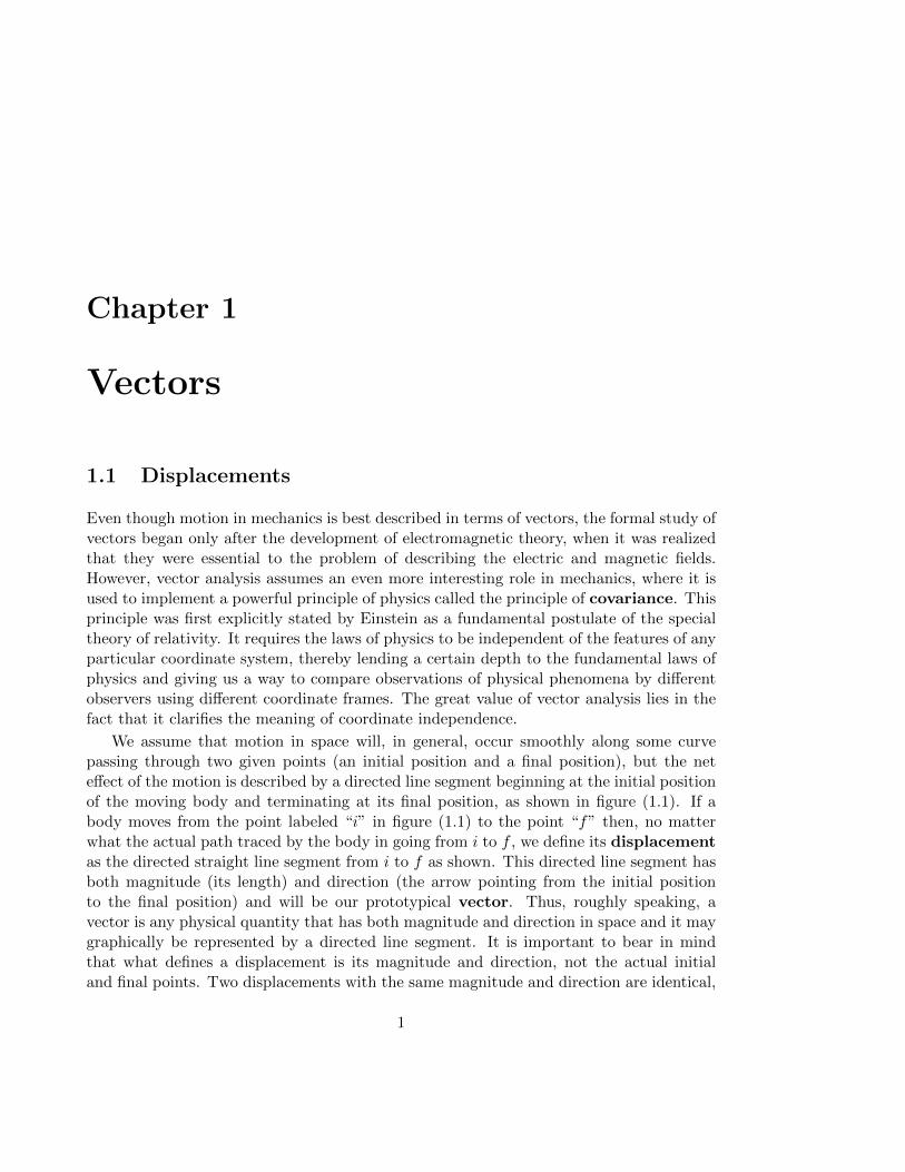
We assume that motion in space will, in general, occur smoothly along some curvepassing through two given points (an initial position and a final position), but the neteffect of the motion is described by a directed line segment beginning at the initial positionof the moving body and terminating at its final position, as shown in figure (1.1). If abody moves from the point labeled “i” in figure (1.1) to the point “f” then, no matterwhat the actual path traced by the body in going from i to f , we define its displacementas the directed straight line segment from i to f as shown. This directed line segment hasboth magnitude (its length) and direction (the arrow pointing from the initial positionto the final position) and will be our prototypical vector. Thus, roughly speaking, avector is any physical quantity that has both magnitude and direction in space and it maygraphically be represented by a directed line segment. It is important to bear in mindthat what defines a displacement is its magnitude and direction, not the actual initialand final points. Two displacements with the same magnitude and direction are identical,
1
2 CHAPTER 1. VECTORS
x1
x3
x2
displacement
i
f
Figure 1.1: Displacement vector
regardless of the initial and final points. So also, what defines a vector is its magnitudeand direction and not its location in space.
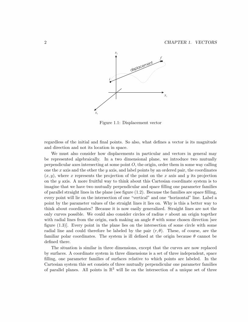
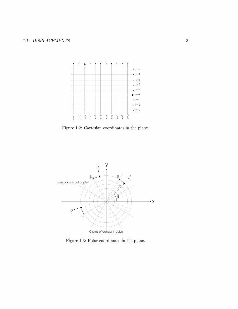
We must also consider how displacements in particular and vectors in general maybe represented algebraically. In a two dimensional plane, we introduce two mutuallyperpendicular axes intersecting at some point O, the origin, order them in some way callingone the x axis and the other the y axis, and label points by an ordered pair, the coordinates(x, y), where x represents the projection of the point on the x axis and y its projectionon the y axis. A more fruitful way to think about this Cartesian coordinate system is toimagine that we have two mutually perpendicular and space filling one parameter familiesof parallel straight lines in the plane (see figure (1.2). Because the families are space filling,every point will lie on the intersection of one “vertical” and one “horizontal” line. Label apoint by the parameter values of the straight lines it lies on. Why is this a better way tothink about coordinates? Because it is now easily generalized. Straight lines are not theonly curves possible. We could also consider circles of radius r about an origin togetherwith radial lines from the origin, each making an angle θ with some chosen direction [seefigure (1.3)]. Every point in the plane lies on the intersection of some circle with someradial line and could therefore be labeled by the pair (r, θ). These, of course, are thefamiliar polar coordinates. The system is ill defined at the origin because θ cannot bedefined there.
The situation is similar in three dimensions, except that the curves are now replacedby surfaces. A coordinate system in three dimensions is a set of three independent, spacefilling, one parameter families of surfaces relative to which points are labeled. In theCartesian system this set consists of three mutually perpendicular one parameter familiesof parallel planes. All points in R3 will lie on the intersection of a unique set of three
1.1. DISPLACEMENTS 3
y=-3
y=-2
y=-1
y=0
y=1
y=2
y=3
y=4
y=5
x=-2
x=-1
x=0
x=1
x=2
x=3
x=4
x=5
x=6
x=7
x=8
Figure 1.2: Cartesian coordinates in the plane.
Lines of constant angle
Circles of constant radius
q
r
r
r
q
x
y
r
Figure 1.3: Polar coordinates in the plane.
4 CHAPTER 1. VECTORS
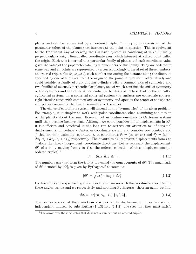
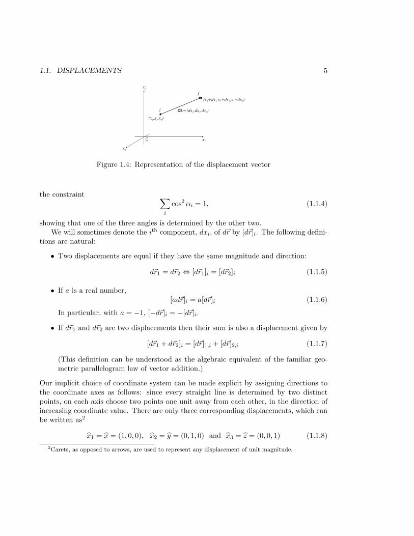
planes and can be represented by an ordered triplet ~r = (x1, x2, x3) consisting of theparameter values of the planes that intersect at the point in question. This is equivalentto the traditional way of viewing the Cartesian system as consisting of three mutuallyperpendicular straight lines, called coordinate axes, which intersect at a fixed point calledthe origin. Each axis is normal to a particular family of planes and each coordinate valuegives the value of the papameter labeling the members of this family. They are ordered insome way and all points are represented by a correspondingly ordered set of three numbers,an ordered triplet ~r = (x1, x2, x3), each number measuring the distance along the directionspecified by one of the axes from the origin to the point in question. Alternatively onecould consider a family of right circular cylinders with a common axis of symmetry andtwo families of mutually perpendicular planes, one of which contains the axis of symmetryof the cylinders and the other is perpendicular to this axis. These lead to the so calledcylindrical system. In a spherical spherical system the surfaces are concentric spheres,right circular cones with common axis of symmetry and apex at the center of the spheresand planes containing the axis of symmetry of the cones.
The choice of coordinate system will depend on the “symmetries” of the given problem.For example, it is simpler to work with polar coordinates when examining the motionof the planets about the sun. However, let us confine ourselves to Cartesian systemsuntil they become inconvenient. Although we could consider finite displacements in R3,it is sufficient and beneficial in the long run to restrict our attention to infinitesimaldisplacements. Introduce a Cartesian coordinate system and consider two points, i andf that are infinitesimally separated, with coordinates ~ri = (x1, x2, x3) and ~rf = (x1 +dx1, x2 + dx2, x3 + dx3) respectively. The quantities dxi represent displacements from i tof along the three (independent) coordinate directions. Let us represent the displacement,d~r, of a body moving from i to f as the ordered collection of these displacements (anordered triplet),1
d~r = (dx1, dx2, dx3). (1.1.1)
The numbers dxi that form the triplet are called the components of d~r. The magnitudeof d~r, denoted by |d~r|, is given by Pythagoras’ theorem as
|d~r| =√dx2
1 + dx22 + dx2
3 . (1.1.2)
Its direction can be specified by the angles that d~r makes with the coordinate axes. Callingthese angles α1, α2 and α3 respectively and applying Pythagoras’ theorem again we find
dxi = |d~r| cosαi, i ∈ 1, 2, 3, (1.1.3)
The cosines are called the direction cosines of the displacement. They are not allindependent. Indeed, by substituting (1.1.3) into (1.1.2), one sees that they must satisfy
1The arrow over the ~r indicates that d~r is not a number but an ordered triplet.
1.1. DISPLACEMENTS 5
x1
x3
x2
ds=(dx ,dx ,dx )1 2 3i
f
(x ,x ,x )1 2 3
(x +dx ,x +dx ,x +dx )1 1 2 2 3 3
0
Figure 1.4: Representation of the displacement vector
the constraint ∑i
cos2 αi = 1, (1.1.4)
showing that one of the three angles is determined by the other two.We will sometimes denote the ith component, dxi, of d~r by [d~r]i. The following defini-
tions are natural:
• Two displacements are equal if they have the same magnitude and direction:
d~r1 = d~r2 ⇔ [d~r1]i = [d~r2]i (1.1.5)
• If a is a real number,[ad~r]i = a[d~r]i (1.1.6)
In particular, with a = −1, [−d~r]i = −[d~r]i.
• If d~r1 and d~r2 are two displacements then their sum is also a displacement given by
[d~r1 + d~r2]i = [d~r]1,i + [d~r]2,i (1.1.7)
(This definition can be understood as the algebraic equivalent of the familiar geo-metric parallelogram law of vector addition.)
Our implicit choice of coordinate system can be made explicit by assigning directions tothe coordinate axes as follows: since every straight line is determined by two distinctpoints, on each axis choose two points one unit away from each other, in the direction ofincreasing coordinate value. There are only three corresponding displacements, which canbe written as2
x1 = x = (1, 0, 0), x2 = y = (0, 1, 0) and x3 = z = (0, 0, 1) (1.1.8)
2Carets, as opposed to arrows, are used to represent any displacement of unit magnitude.
6 CHAPTER 1. VECTORS
and it is straightforward that, using the scalar multiplication rule (1.1.6) and the sum rule(1.1.7), any displacement d~r could also be represented as
d~r = dx1x1 + dx2x2 + dx3x3 =∑i
dxixi. (1.1.9)
The xi represent unit displacements along the of our chosen Cartesian system and theset xi is called a basis. In R3, we could use the Cartesian coordinates of any point torepresent its displacement from the origin. Displacements in R3 from the origin
~r = (x1, x2, x3) =∑i
xixi. (1.1.10)
are called position vectors.It is extremely important to recognize that the representation of a displacement de-
pends sensitively on the choice of coordinate system whereas the displacement itself doesnot. Therefore, we must distinguish between displacements (and, vectors, in general)and their representations. To see why this is important, we first examine how differentCartesian systems transform into one another.
1.2 Linear Coordinate Transformations
Two types of transformations exist between Cartesian frames, viz., translations of theorigin of coordinates and rotations of the axes. Translations are just constant shifts ofthe coordinate origin. If the origin, O, is shifted to the point O′ whose coordinates are(xO, yO, zO), measured from O, the coordinates get likewise shifted, each by the corre-sponding constant,
x′ = x− xO, y′ = y − yO, z′ = z − zO (1.2.1)
But since xO, yO and zO are all constants, such a transformation does not change therepresentation of a displacement vector,
d~r = (dx, dy, dz) = (dx′, dy′, dz′). (1.2.2)
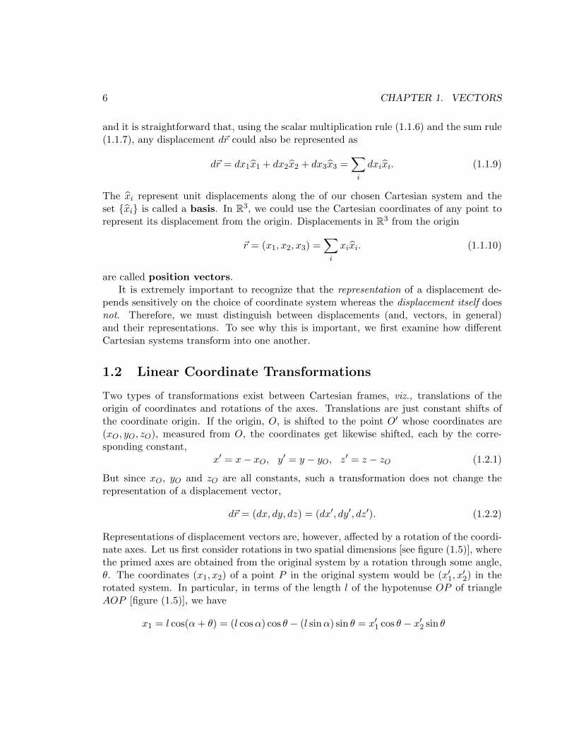
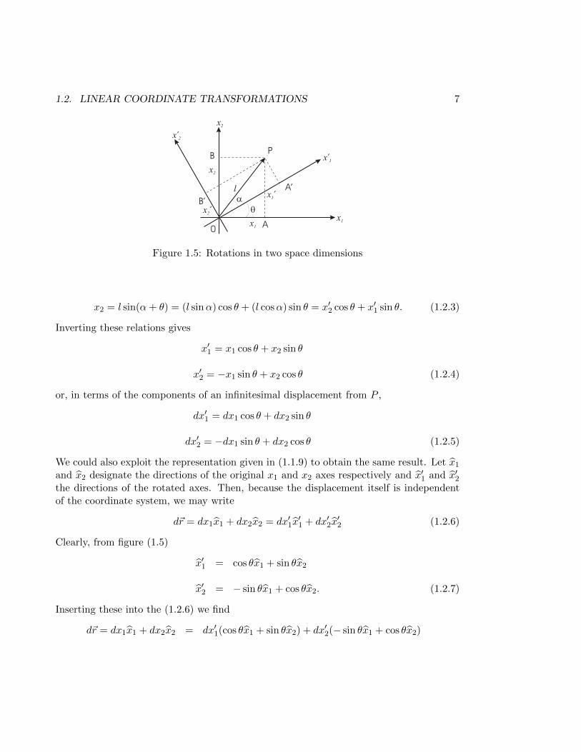
Representations of displacement vectors are, however, affected by a rotation of the coordi-nate axes. Let us first consider rotations in two spatial dimensions [see figure (1.5)], wherethe primed axes are obtained from the original system by a rotation through some angle,θ. The coordinates (x1, x2) of a point P in the original system would be (x′1, x
′2) in the
rotated system. In particular, in terms of the length l of the hypotenuse OP of triangleAOP [figure (1.5)], we have
x1 = l cos(α+ θ) = (l cosα) cos θ − (l sinα) sin θ = x′1 cos θ − x′2 sin θ
1.2. LINEAR COORDINATE TRANSFORMATIONS 7
x1
x’1
x2
x’2
P
q
0
A’
A
B
B’
l
a
x1
x2
x2’
x1’
Figure 1.5: Rotations in two space dimensions
x2 = l sin(α+ θ) = (l sinα) cos θ + (l cosα) sin θ = x′2 cos θ + x′1 sin θ. (1.2.3)
Inverting these relations gives
x′1 = x1 cos θ + x2 sin θ
x′2 = −x1 sin θ + x2 cos θ (1.2.4)
or, in terms of the components of an infinitesimal displacement from P ,
dx′1 = dx1 cos θ + dx2 sin θ
dx′2 = −dx1 sin θ + dx2 cos θ (1.2.5)
We could also exploit the representation given in (1.1.9) to obtain the same result. Let x1
and x2 designate the directions of the original x1 and x2 axes respectively and x′1 and x′2the directions of the rotated axes. Then, because the displacement itself is independentof the coordinate system, we may write
d~r = dx1x1 + dx2x2 = dx′1x′1 + dx′2x
′2 (1.2.6)
Clearly, from figure (1.5)
x′1 = cos θx1 + sin θx2
x′2 = − sin θx1 + cos θx2. (1.2.7)
Inserting these into the (1.2.6) we find
d~r = dx1x1 + dx2x2 = dx′1(cos θx1 + sin θx2) + dx′2(− sin θx1 + cos θx2)
8 CHAPTER 1. VECTORS
= (dx′1 cos θ − dx′2 sin θ)x1 + (dx′1 sin θ + dx′2 cos θ)x2 (1.2.8)
A simple comparison now gives
dx1 = dx′1 cos θ − dx′2 sin θ
dx2 = dx′1 sin θ + dx′2 cos θ (1.2.9)
or, upon inverting the relations,
dx′1 = dx1 cos θ + dx2 sin θ
dx′2 = −dx1 sin θ + dx2 cos θ. (1.2.10)
It is easy to see that these transformations can also be written in matrix form as(dx′1dx′2
)=
(cos θ sin θ− sin θ cos θ
)(dx1
dx2
)(1.2.11)
and (dx1
dx2
)=
(cos θ − sin θsin θ cos θ
)(dx′1dx′2
)(1.2.12)
Other, more complicated but rigid transformations of the coordinate system can alwaysbe represented as combinations of rotations and translations.
1.3 Vectors and Scalars
Definition: A vector is a quantity that can be represented in a Cartesian system byan ordered triplet (A1, A2, A3) of components, which transform as the components of aninfinitesimal displacement under a rotation of the reference coordinate system. Any vectorcan always be expressed as a linear combination of basis vectors, ~A = Aixi.
In two dimensions, a vector may be represented by two Cartesian components ~A =(A1, A2), which transform under a rotation of the Cartesian reference system as (A1, A2)→(A′1, A
′2) such that (
A′1A′2
)=
(cos θ sin θ− sin θ cos θ
)(A1
A2
)(1.3.1)
Definition: A scalar is any physical quantity that does not transform (stays invariant)under a rotation of the reference coordinate system.
1.4. ROTATIONS IN TWO DIMENSIONS 9
A typical scalar quantity in Newtonian mechanics would be the mass of a particle. Themagnitude of a vector is also a scalar quantity, as we shall soon see. It is of great interestto determine scalar quantities in physics because these quantities are not sensitive toparticular choices of coordinate systems and are therefore the same for all observers.Other examples of scalars within the context of Newtonian mechanics are temperatureand density.
In the Newtonian conception of space and time, time is also a scalar. Because time isa scalar all quantities constructed from the position vector of a particle moving in spaceby taking derivatives with respect to time are also vectors, therefore
• the velocity: ~v = d~rdt
• the acceleration: ~a = d~vdt
• the momentum: ~p = m~v and
• the force ~F = d~pdt
are all examples of vectors that arise naturally in mechanics. In electromagnetism, theelectric and magnetic fields are vectors. As an example of a quantity that has the ap-pearance of a vector but is not a vector, consider A = (x,−y). Under a rotation of thecoordinate system by an angle θ,
A′1 = A1 cos θ −A2 sin θ
A′2 = A1 sin θ +A2 cos θ (1.3.2)
which are not consistent with (1.3.1). The lesson is that the transformation propertiesmust always be checked.
1.4 Rotations in two dimensions
Equation (1.3.1) can also be written as follows
A′i =∑j
RijAj (1.4.1)
where
Rij(θ) =
(cos θ sin θ− sin θ cos θ
)(1.4.2)
is just the two dimensional “rotation” matrix. We easily verify that it satisfies the followingvery interesting properties:
10 CHAPTER 1. VECTORS
1. If we perform two successive rotations on a vector ~A, so that after the first rotation
Ai → A′i =∑j
Rij(θ1)Aj (1.4.3)
and after the second rotation
A′i → Ai′′ =
∑k
Rik(θ2)A′k =∑k
Rik(θ2)Rkj(θ1)Aj (1.4.4)
then by explicit calculation it follows that∑k
Rik(θ2)Rkj(θ1) = Rij(θ1 + θ2) (1.4.5)
soAi′′ =
∑j
Rij(θ1 + θ2)Aj (1.4.6)
i.e., the result of two rotations is another rotation. The set of rotation matrices istherefore “closed” under matrix multiplication.
2. The unit matrix, 1, is the rotation matrix R(0).
3. The transpose of the rotation matrix whose angle is θ is the rotation matrix whoseangle is −θ. This follows easily from,
R(−θ) =
(cos(−θ) sin(−θ)− sin(−θ) cos(−θ)
)=
(cos θ − sin θsin θ cos θ
)= RT (θ) (1.4.7)
Now, using the closure property,
RT (θ) ·R(θ) = R(−θ) ·R(θ) = R(0) = 1 (1.4.8)
Therefore, for every rotation matrix R(θ) there exists an inverse, R(−θ) = RT .
4. Matrix multiplication is associative.
The rotation matrices therefore form a group under matrix multiplication.3 The groupelements are all determined by one continuous parameter, the rotation angle θ. This isthe commutative group, called SO(2), of 2 × 2 orthogonal matrices with unit determi-nant, under matrix multiplication. We will now see that the situation gets vastly morecomplicated in the physically relevant case of three dimensions.
3Recall the following definitions:
Definition: The pair (G, ∗) consisting of any set G = g1, g2, ... with a binary operation ∗ defined on itthat obeys the four properties
• closure under ∗, i.e., ∀ g1, g2 ∈ G g1 ∗ g2 ∈ G• existence of an identity, i.e., ∃ e ∈ G s.t. ∀ g ∈ G, g ∗ e = e ∗ g = g
1.5. ROTATIONS IN THREE DIMENSIONS 11
1.5 Rotations in three dimensions
In two dimensions there is just one way to rotate the axes which, if we introduce a “x3”axis, amounts to a rotation of the x1−x2 axes about it. In three dimensions there are threesuch rotations possible: the rotation of the x1 − x2 axes about the x3 axis, the rotationof the x2 − x3 axes about the x1 axis and the rotation of the x1 − x3 axes about the x2
axis. In each of these rotations the axis of rotation remains fixed, and each rotation isobviously independent of the others. Thus, we now need 3× 3 matrices and may write
R3(θ) =
cos θ sin θ 0− sin θ cos θ 0
0 0 1
(1.5.1)
to represent the rotation of the x1 − x2 axes as before about the x3 axis. Under such arotation only the first and second component of a vector are transformed according to therule
A′i =∑j
R3ij(θ)Aj (1.5.2)
Rotations about the other two axes may be written likewise as follows:
R1(θ) =
1 0 00 cos θ sin θ0 − sin θ cos θ
(1.5.3)
and4
R2(θ) =
cos θ 0 − sin θ0 1 0
sin θ 0 cos θ
(1.5.4)
The general rotation matrix in three dimensions may be constructed in many ways, oneof which (originally due to Euler) is canonical:
• first rotate the (x1, x2) about the x3 axis through an angle θ. This gives the newaxes (ξ, η, τ) (τ ≡ z),
• existence of an inverse i.e., ∀ g ∈ G ∃ g−1 ∈ G s.t. g ∗ g−1 = g−1 ∗ g = e, and
• associativity of ∗, i.e., ∀ g1, g2, g3 ∈ G, g1 ∗ (g2 ∗ g3) = (g1 ∗ g2) ∗ g3is called a group.
Definition: If ∀ g1, g2 ∈ G, [g1, g2] = g1 ∗ g2 − g2 ∗ g1 = 0 then the group (G, ∗) is called a “commutative”or “ Abelian” group. [g1, g2] is called the commutator of the elements g1 and g2.
4Note the change in sign. It is because we are using a right-handed coordinate system. Convinceyourself that it should be so.
12 CHAPTER 1. VECTORS
• then rotate (ξ, η, z) about the ξ axis through an angle φ. This gives the new axes(ξ′, η′, τ ′) (ξ′ ≡ ξ),
• finally rotate (ξ, η′, τ ′) about the τ ′ axis through an angle ψ to get (x′, y′, z′).
We getR(θ, φ, ψ) = R3(ψ) · R2(φ) · R3(θ) (1.5.5)
The angles θ, φ, ψ are called the Euler angles after the the originator of this particularsequence of rotations.5 The sequence is not unique however and there are many possibleways to make a general rotation. To count the number of ways, we need to keep in mindthat three independent rotations are necessary:
• the first rotation can be performed in one of three ways, corresponding to the threeindependent rotations about the axes,
• the second rotation can be performed in one of two independent ways: we are not per-mitted to rotate about the axis around which the previous rotation was performed,and
• the third rotation can be performed in one of two independent ways: again weare not permitted to rotate about the axis around which the previous rotation wasperformed.
So in all there are 3 × 2 × 2 = 12 possible combinations of rotations that will give thedesired general rotation matrix in three dimensions. Note that any scheme you choosewill involve three and only three independent angles, whereas only one angle was neededto define the general rotation matrix in two dimensions. The general rotation matrix in ndimensions will require n(n− 1)/2 angles.
Three dimensional rotation matrices satisfy some interesting properties that we willnow outline:
• The product of any two rotation matrices is also a rotation matrix.
• The identity matrix is just the rotation matrix R(0, 0, 0).
• All three dimensional rotation matrices, like their two dimensional counterparts,obey the condition
RT · R = 1 (1.5.6)
5Problem: Show that the general rotation matrix constructed with the Euler angles is
R(θ, φ, ψ) =
cosψ cos θ − cosφ sin θ sinψ cosψ sin θ + cosφ cos θ sinψ sinψ sinφ− sinψ cos θ − cosφ sin θ cosψ − sinψ sin θ + cosφ cos θ cosψ cosψ sinφ
sinφ sin θ − sinφ cos θ cosφ
1.5. ROTATIONS IN THREE DIMENSIONS 13
where RT is the transpose of R, i.e.,
RTij = Rji (1.5.7)
The transpose of any rotation matrix is also a rotation matrix. It is obtained byapplying the separate rotation matrices in reverse order. In the Euler parametriza-tion,6
RT (θ, φ, ψ) = R(−ψ,−φ,−θ) (1.5.8)
Therefore, the transpose of a rotation matrix is its inverse.
• Finally, the associative property of matrix multiplication ensures that the productof rotations is associative.
The four properties listed above ensure that three dimensional rotations form a group un-der matrix multiplication. This the continuous, three parameter group called SO(3) and isthe group of all 3×3 orthogonal matrices of unit determinant, under matrix multiplication.The group is not commutative.
Rotations keep the magnitude of a vector invariant. Suppose ~A has components(A1, A2, A3). Under a general rotation the components transform as
A′i =∑j
RijAj (1.5.9)
Therefore,∑i
A′iA′i =
∑ijk
AjRTjiRikAk =
∑jk
Aj
(∑i
RTjiRik
)Ak =
∑jk
AjδjkAk =∑j
AjAj
(1.5.10)where δjk is the Kronecker δ,7 and in the last step we use the fact that the transpose of
R is its inverse.∑
iAiAi is simply the length square of the vector | ~A|, or its magnitudesquared, i.e.,
| ~A| =√∑
i
AiAi (1.5.11)
6Problem: Verify this explicitly!7Problem: The Kronecker δ is defined by
δij =
0 if i 6= j1 if i = j
so it is the unit matrix. In fact, δij is a “tensor”, i.e., it transforms as two copies of a vector underrotations. Show this by showing that
δ′ij =∑lk
RilRjkδlk = δij .
14 CHAPTER 1. VECTORS
is invariant under rotations.
1.6 Algebraic Operations on Vectors
We define
• Vector equality:~A = ~B ⇔ Ai = Bi, for all i (1.6.1)
• Scalar multiplication:
~B = a ~A⇔ Bi = aAi, for a ∈ R (1.6.2)
and
• Vector addition/subtraction:
~C = ~A± ~B ⇔ Ci = Ai ±Bi (1.6.3)
It is easy to show that the results of scalar multiplication, addition and subtraction arevectors (i.e., having the correct transformation properties). Furthermore, there are twoways to define a product between two vectors.
1.6.1 The scalar product
The first is called the scalar (or inner, or dot) product and yields a scalar quantity. If ~Aand ~B are two vectors,
~A · ~B =∑i
AiBi (1.6.4)
To show that ~A · ~B is a scalar under rotations, consider∑i
A′iB′i =
∑ijk
AjRTjiRikBk =
∑jk
AjδjkBk =∑j
AjBj . (1.6.5)
Notice that | ~A| =√~A · ~A.
The basis vectors xi satisfy xi · xj = δij and the component of a vector ~A along
any of the axes can be obtained from the scalar product of ~A with the unit vector in thedirection of the axis,
Ai = ~A · xi, (1.6.6)
1.6. ALGEBRAIC OPERATIONS ON VECTORS 15
Since Ai = | ~A| cosαi, it can be used to define the direction cosines,
cosαi =~A · xi| ~A|
=~A · xi√~A · ~A
(1.6.7)
Indeed, if u is any unit vector, the component of ~A in the direction of u is Au = ~A · u.Because the scalar product is invariant under rotations, we prove this by letting αi bethe direction angles of ~A and βi be the direction angles of u in the particular frame inwhich both ~A and u lie in the x1 − x2 plane (such a plane can always be found). Thenα3 = β3 = π
2 and
~A · u = | ~A|∑i
cosαi cosβi = | ~A|(cosα1 cosβ1 + cosα2 cosβ2) (1.6.8)
In two dimensions, α2 = π2 − α1 and β2 = π
2 − β1 so
~A · u = | ~A|(cosα1 cosβ1 + sinα1 sinβ1) = | ~A| cos(α1 − β1) = | ~A| cos θu (1.6.9)
where θu is the angle between ~A and u, because α1 and β1 are the angles made with the xaxis. It follows, by Pythagoras’ theorem, that Au is the component of ~A in the directionof u. In a general coordinate frame, for any two vectors ~A and ~B,
~A · ~B = | ~A|| ~B|∑i
cosαi cosβi = | ~A|| ~B| cos θAB (1.6.10)
where θAB is the angle between ~A and ~B.
1.6.2 The vector product
The second product between two vectors yields another vector and is called the vector (orcross) product. If ~C = ~A× ~B, then
Ci =∑jk
εijkAjBk (1.6.11)
where we have introduced the three index quantity called the Levi-Civita tensor (density),defined by8
εijk =
+1 if i, j, k is an even permutation of 1, 2, 3−1 if i, j, k is an odd permutation of 1, 2, 30 if i, j, k is not a permutation of 1, 2, 3
(1.6.12)
8Prove that εijk transforms as a rank three tensor, i.e., according to three copies of a vector. Show that
ε′ijk =∑lmn
RilRjmRknεlmn = εijk
provided that the rotation matrices are of unit determinant.
16 CHAPTER 1. VECTORS
eijk+1
1
2 3
-1
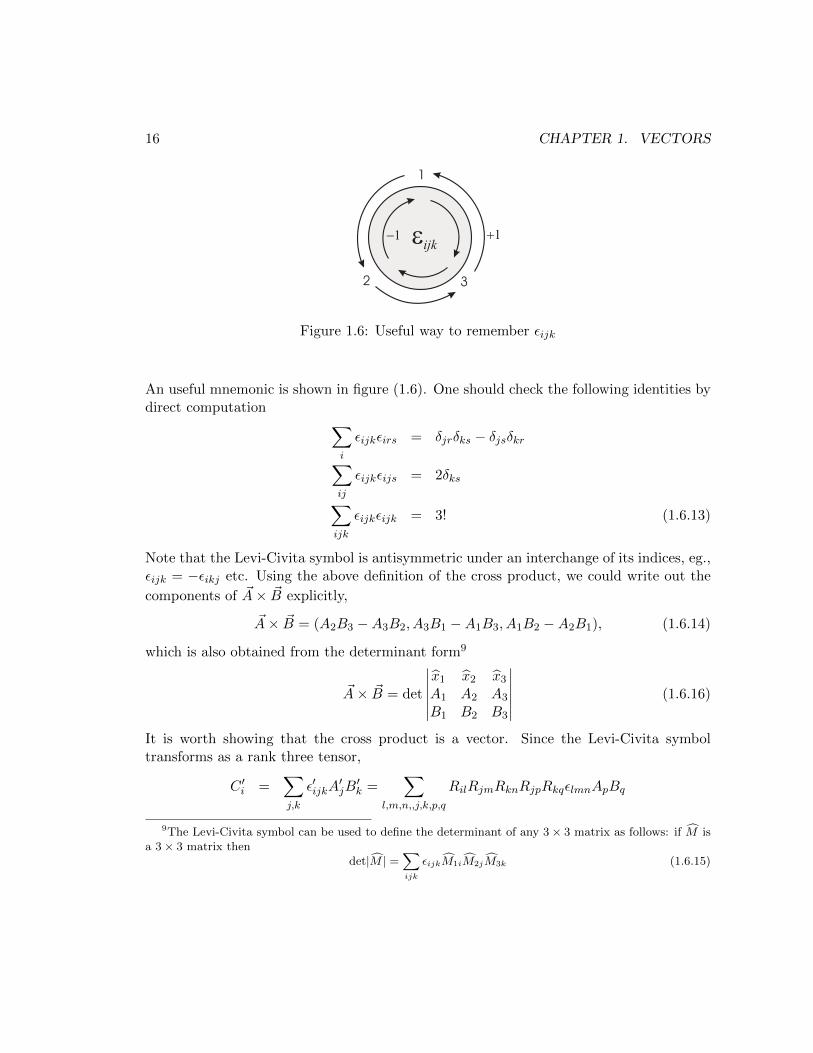
Figure 1.6: Useful way to remember εijk
An useful mnemonic is shown in figure (1.6). One should check the following identities bydirect computation ∑
i
εijkεirs = δjrδks − δjsδkr∑ij
εijkεijs = 2δks∑ijk
εijkεijk = 3! (1.6.13)
Note that the Levi-Civita symbol is antisymmetric under an interchange of its indices, eg.,εijk = −εikj etc. Using the above definition of the cross product, we could write out the
components of ~A× ~B explicitly,
~A× ~B = (A2B3 −A3B2, A3B1 −A1B3, A1B2 −A2B1), (1.6.14)
which is also obtained from the determinant form9
~A× ~B = det
∣∣∣∣∣∣x1 x2 x3
A1 A2 A3
B1 B2 B3
∣∣∣∣∣∣ (1.6.16)
It is worth showing that the cross product is a vector. Since the Levi-Civita symboltransforms as a rank three tensor,
C ′i =∑j,k
ε′ijkA′jB′k =
∑l,m,n,,j,k,p,q
RilRjmRknRjpRkqεlmnApBq
9The Levi-Civita symbol can be used to define the determinant of any 3× 3 matrix as follows: if M isa 3× 3 matrix then
det|M | =∑ijk
εijkM1iM2jM3k (1.6.15)
1.7. VECTOR SPACES 17
A
B
A X B
Figure 1.7: The right hand rule
=∑l,m,n
RilεlmnAmBn =∑l
RilCl (1.6.17)
where we have used∑
k RknRkq = δnq and∑
j RjmRjp = δmp.
Notice that ~A× ~A = 0 and that the basis vectors obey xi× xj = εijkxk. In a coordinate
frame that has been rotated so that both ~A and ~B lie in the x1−x2 plane, using cosα2 =sinα1 and cosβ2 = sinβ1 together with cosα3 = cosβ3 = 0, we find that the only non-vanishing component of ~C is C3 given by
C3 = | ~A|| ~B|(cosα1 sinβ1 − sinα1 cosβ1) = | ~A|| ~B| sin(β1 − α1) (1.6.18)
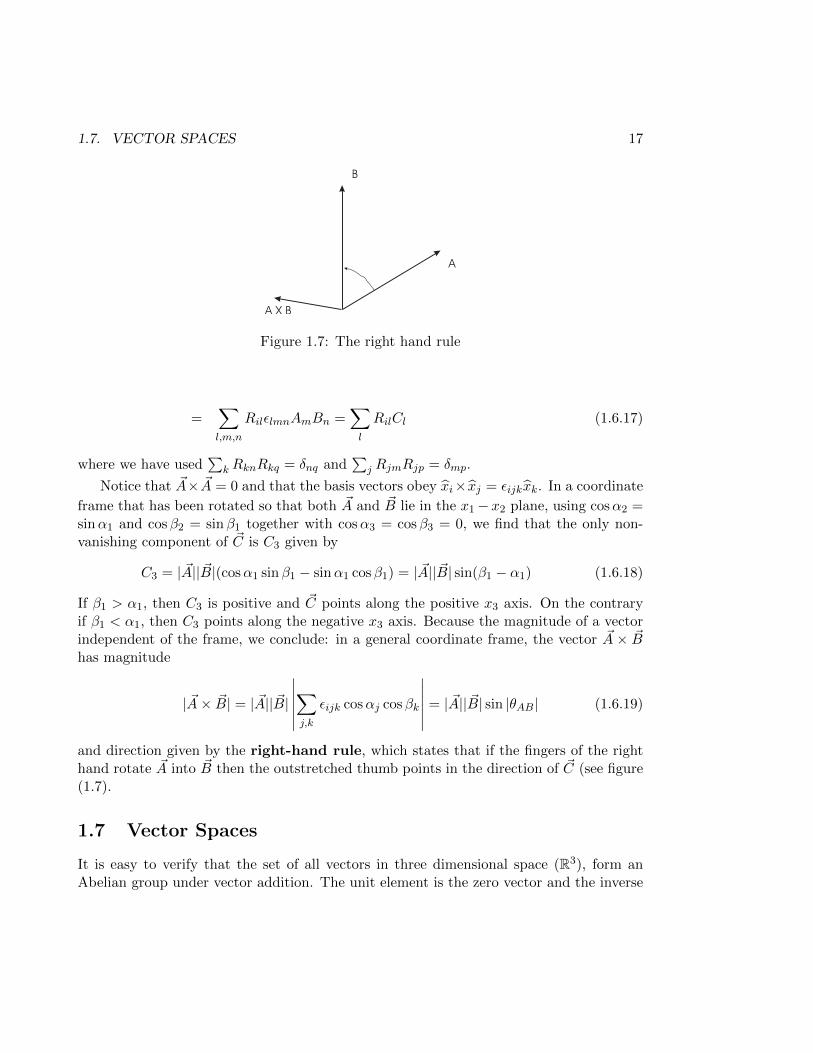
If β1 > α1, then C3 is positive and ~C points along the positive x3 axis. On the contraryif β1 < α1, then C3 points along the negative x3 axis. Because the magnitude of a vectorindependent of the frame, we conclude: in a general coordinate frame, the vector ~A × ~Bhas magnitude
| ~A× ~B| = | ~A|| ~B|
∣∣∣∣∣∣∑j,k
εijk cosαj cosβk
∣∣∣∣∣∣ = | ~A|| ~B| sin |θAB| (1.6.19)
and direction given by the right-hand rule, which states that if the fingers of the righthand rotate ~A into ~B then the outstretched thumb points in the direction of ~C (see figure(1.7).
1.7 Vector Spaces
It is easy to verify that the set of all vectors in three dimensional space (R3), form anAbelian group under vector addition. The unit element is the zero vector and the inverse
18 CHAPTER 1. VECTORS
of ~A is − ~A. Moreover, vector addition inherits its associativity from addition of ordinarynumbers and is commutative. The space is also closed under scalar multiplication, sincemultiplying any vector by a real number gives another vector. Scalar multiplication is also
• associative,
a(b ~A) = (ab) ~A, (1.7.1)
• distributive over vector addition,
a( ~A+ ~B) = a ~A+ a ~B (1.7.2)
• as well as over scalar addition,
(a+ b) ~A = a ~A+ b ~B, (1.7.3)
• and admits an identity (1),
1( ~A) = ~A (1.7.4)
In general, a vector space is any set that is a group under some binary operation (addition)over which multiplication by elements of a field, satisfying the four properties listed above,is defined.10 Although we have considered only scalar multiplication by real numbers,scalar multiplication by elements of any field (eg. the complex numbers or the rationalnumbers) is possible in general. The scalar and vector products we have defined areadditional structures, not inherent to the definition of a vector space. The vectors we haveintroduced are geometric vectors in R3.
1.8 Some Algebraic Identities
We turn to proving some simple but important identities involving the scalar and vectorproducts. The examples given will not be exhaustive, but will serve to illustrate the general
10 Additional Definitions:
• A set of vectors, ~Ai, is linearly independent if for scalars ai,∑i
ai ~Ai = 0⇔ ai = 0 ∀ i.
• A set of linearly independent vectors is complete if any vector in the vector space may be expressedas a linear combination of its members.
• A complete set of linearly independent vectors is said to form a basis for the vector space.
• The set of vectors x1 = (1, 0, 0), x2 = (0, 1, 0) and x3 = (0, 0, 1), form a basis for R3.
1.8. SOME ALGEBRAIC IDENTITIES 19
methods used. To simplify notation we will henceforth employ the following convention:if an index is repeated in any expression, it is automatically assumed that the index is tobe summed over. Thus we will no longer write the sums explicitly (this is known as theEinstein summation convention).
1. ~A× ~B = − ~B × ~A.We prove this for the components.
[ ~A× ~B]i = εijkAjBk = εikjAkBj = εikjBjAk = −εijkBjAk = −[ ~B × ~A]i
where, in the second step, we have simply renamed the indices by calling j ↔ kwhich changes nothing as the indices j and k are summed over. In the next to laststep we have used the fact that εijk is antisymmetric in its indices, so that everyinterchange of indices in εijk introduces a negative sign.
2. ~A× ( ~B × ~C) = ( ~A · ~C) ~B − ( ~A · ~B)~CAgain take a look at the components,
[ ~A× ( ~B × ~C)]i = εijkAj [ ~B × ~C]k = εijkεklmAjBlCm
= εijkεlmkAjBlCm = (δilδjm − δimδjl)AjBlCm
= ( ~A · ~C)Bi − ( ~A · ~B)Ci
3. ( ~A× ~B) · (~C × ~D) = ( ~A · ~C)( ~B · ~D)− ( ~A · ~D)( ~B · ~C)Write everything down in components. The left hand side is
( ~A× ~B) · (~C × ~D) = εijkAjBkεilmClDm = (δjlδkm − δjmδkl)AjBkClDm
= ( ~A · ~C)( ~B · ~D)− ( ~A · ~D)( ~B · ~C)
In particular, ( ~A× ~B)2 = ~A2 ~B2 sin2 θ, where θ is the angle between ~A and ~B.
4. The triple product of three vectors ~A, ~B and ~C is defined by
[ ~A, ~B, ~C] = ~A · ( ~B × ~C) = εijkAiBjCk
This is a scalar.11 It satisfies the following properties:
[ ~A, ~B, ~C] = [~C, ~A, ~B] = [ ~B, ~C, ~A] = −[ ~B, ~A, ~C] = −[~C, ~B, ~A] = −[ ~A, ~C, ~B] (1.8.1)
i.e., the triple product is even under cyclic permutations and otherwise odd. Also[ ~A, ~A, ~B] = 0. All these properties follow directly from the properties of the Levi-Civita tensor density, εijk.
12
11Problem: Verify this!12Problem: Convince yourself that this is so.
20 CHAPTER 1. VECTORS
5. ( ~A× ~B)× (~C × ~D) = [ ~A, ~B, ~D]~C − [ ~A, ~B, ~C] ~DThe left hand side is just
( ~A× ~B)× (~C × ~D) = εijkεjrsεkmnArBsCmDn = εjrs(δimδjn − δinδjm)ArBsCmDn
= (εnrsArBsDn)Ci − (εmrsArBsCm)Di
= [ ~A, ~B, ~D]~C − [ ~A, ~B, ~C] ~D
1.9 Differentiation of Vectors
1.9.1 Time derivatives
A vector function of time is a vector whose components are functions of time. The deriva-tive of a vector function of time is then defined in a natural way in terms of the derivativesof its components in the Cartesian basis. Let ~A(t) be a vector function of some parametert, i.e.,
~A(t) = (A1(t), A2(t), A3(t)) (1.9.1)
The derivative of ~A(t) is another vector function, ~C(t), whose Cartesian components aregiven by
Ci =dAidt
(1.9.2)
Note that the above definition is “good” only in for the Cartesian components of thevector. This is because the Cartesian basis xi is rigid, i.e., it does not change in space.In more general coordinate systems, where the basis is not rigid, the derivative of a vectormust be handled delicately. We will return to this later. Here, we will convince ourselvesthat ~C is really a vector. Under a rotation
Ai → A′i ⇒ C ′i =dA′idt
=d
dt(RijAj) = Rij
dAidt
= RijCj (1.9.3)
which shows that ~C(t) has the correct transformation properties, inherited from ~A(t).This justifies the statement that the velocity, momentum, acceleration and force must allbe vectors, because they are all obtained by differentiating ~r(t).13
13Problem: Show that
dr
dt= r · ~v
dr
dt=~v
r− r
r(r · ~v)
where r = |~r|, r is the unit position vector and ~v is the velocity vector.
1.9. DIFFERENTIATION OF VECTORS 21
1.9.2 The Gradient Operator
The gradient operator is a vector differential operator, whose definition is motivatedby a simple geometric fact. Consider some scalar function φ(~r)14 and the surface in R3,defined by
φ(~r) = φ(x1, x2, x3) = const., (1.9.4)
so that
φ′(x′1, x′2, x′3) = φ(x1, x2, x3) (1.9.5)
The total differential of φ(~r) is given by
dφ =∂φ
∂x1dx1 +
∂φ
∂x2dx2 +
∂φ
∂x3dx3, (1.9.6)
which can be re-expressed as
dφ =
(∂φ
∂x1,∂φ
∂x2,∂φ
∂x3
)· (dx1, dx2, dx3) = 0. (1.9.7)
The vector (dx1, dx2, dx3) represents an infinitesimal displacement on the surface deter-mined by the equation φ(x1, x2, x3) = const. The other vector in the scalar product iscalled the gradient of the function φ(~r),
~∇φ =
(∂φ
∂x1,∂φ
∂x2,∂φ
∂x3
)(1.9.8)
It has the form of a vector, but we need to check of course that its transformation propertiesunder rotations are those of a vector. We will therefore look at the components of ~∇φ:
∂φ
∂xi= ∂iφ→ ∂′iφ
′ =∂φ′
∂x′i=
∂φ
∂xj
∂xj∂x′i
(1.9.9)
Now
x′i = Rikxk ⇒ xj = RTjixi (1.9.10)
so∂xj∂x′i
= RTji = Rij (1.9.11)
and therefore
∂′iφ′ =
∂φ′
∂x′i= Rij∂jφ (1.9.12)
14Any scalar function φ(~r, t) is called a scalar field.
22 CHAPTER 1. VECTORS
which is indeed the vector transformation law. Hence ~∇φ is a vector if φ(~r) is a scalar.Now it turns out that ~∇φ has a nice geometric meaning. Because
~∇φ · d~r = 0 (1.9.13)
for all infinitesimal displacements along the surface, it follows that ~∇φ, if it is not vanishing,must be normal to the surface given by φ(~r) = const. Thus, given any surface φ(~r) =const.,
n =~∇φ|~∇φ|
(1.9.14)
is the unit normal to the surface.
Example: Take φ(x, y, z) = x2 + y2 + z2, then φ(~r) = const. represents a sphere centeredat the origin of coordinates. The unit normal to the sphere at any point is
~∇φ =~r
r(1.9.15)
where r is the radius of the sphere and ~r is the position vector of the point. The normalto the sphere is therefore in the direction of the radius.
Example: Take φ(x, y, z) = x2
a2+ y2
b2+ z2
c2, so that φ(x, y, z) = 1 represents an ellipsoid with
semi-axes of lengths a, b and c respectively. We find
n = (x
a,y
b,z
c) (1.9.16)
which is the normal to the ellipsoid at the point (x, y, z).
We see that ~∇ is just the derivative operator in the Cartesian system, so we can think ofit in component form as the collection of derivatives,
[~∇]i = ∂i. (1.9.17)
Now if we introduce the concept of a vector field as a vector function of space and time,
~A(~r, t) = (A1(~r, t), A2(~r, t), A3(~r, t)) (1.9.18)
then we can define two distinct operations on ~A(~r, t) using the scalar and vector productsgiven earlier,
• the divergence of a vector field ~A(~r, t) as
div ~A = ~∇ · ~A = ∂iAi (1.9.19)
and
1.10. SOME DIFFERENTIAL IDENTITIES 23
• the curl (or rotation) of a vector field ~A(~r, t) as
[~∇× ~A]i = εijk∂jAk (1.9.20)
These turn out to be of fundamental importance in any dynamical theory of fields, eg.,electromagnetism. We will understand their physical significance in the following chapters.For now, we only prove a few identities involving the ~∇ operator. Once again, the examplesgiven are far from exhaustive, their purpose being only to illustrate the method.
1.10 Some Differential Identities
1. ~∇ · ~r = 3This follows directly from the definition of the divergence,
~∇ · ~r = ∂ixi = δii = 3
2. ~∇ · (φ ~A) = (~∇φ) · ~A+ φ(∇ · ~A)Expand the l.h.s to get
∂i(φAi) = (∂iφ)Ai + φ(∂iAi) = (~∇φ) · ~A+ φ(∇ · ~A) (1.10.1)
As a special case, take ~A = ~r, then ~∇ · (~rφ) = ~r · (~∇φ) + 3φ
3. ~∇ · (~∇× ~A) ≡ 0The proof is straightforward and relies on the antisymmetry of εijk:
~∇ · (~∇× ~A) = εijk∂i∂jAk = 0
which follows because ∂i∂j is symmetric w.r.t. ij while εijk is antisymmetric w.r.t.the same pair of indices.
4. ~∇ · ( ~A× ~B) = (~∇× ~A) · ~B − ~A · (~∇× ~B)Expanding the l.h.s.,
∂i(εijkAjBk) = εijk[(∂iAj)Bk +Aj(∂iBk)]
= (εkij∂iAj)Bk −Aj(εjik∂iBk)
= (~∇× ~A) · ~B − ~A · (~∇× ~B)
5. ~∇× ~r = 0This also follows from the antisymmetry of the Levi-Civita tensor,
~∇× ~r = εijk∂jxk = εijkδjk = 0
24 CHAPTER 1. VECTORS
6. ~∇× ~∇φ ≡ 0This is another consequence of the same reasoning as above,
~∇× ~∇φ = εijk∂j∂kφ = 0
7. ~∇× (φ ~A) = (~∇φ)× ~A+ φ(∇× ~A)Consider the ith component of the l.h.s.,
[~∇× (φ ~A)]i = εijk∂j(φAk) = εijk(∂jφ)Ak + εijkφ(∂jAk)
= [~∇φ× ~A]i + φ[~∇× ~A]i
As a special case, take ~A = ~r, then ~∇× (~rφ) = (~∇φ)× ~r.
8. ~∇× (~∇× ~A) = ~∇(~∇ · ~A)− ~∇2 ~ABeginning with,
[~∇× (~∇× ~A)]i = εijk∂j(εklm∂lAm) = (δilδjm − δimδjl)∂j∂lAm
= ∂i(∂mAm)− ∂j∂jAi = [~∇(~∇ · ~A)]i − [~∇2 ~A]i
9. ~∇× ( ~A× ~B) = (~∇ · ~B) ~A− (~∇ · ~A) ~B + ( ~B · ~∇) ~A− ( ~A · ~∇) ~BAgain, beginning with,
[~∇× ( ~A× ~B)]i = εijkεklm∂j(AlBm) = (δilδjm − δimδjl)∂j(AlBm)
= ∂j(AiBj)− ∂j(AjBi)
= (∂jBj)Ai + (Bj∂j)Ai − (∂jAj)Bi − (Aj∂j)Bi
= (~∇ · ~B)[ ~A]i − (~∇ · ~A)[ ~B]i + ( ~B · ~∇)[ ~A]i − ( ~A · ~∇)[ ~B]i
10. ~∇( ~A · ~B) = ( ~A · ~∇) ~B + ( ~B · ~∇) ~A+ ~A× (~∇× ~B) + ~B × (~∇× ~A)Consider the ith component of the last two terms on the right,
[ ~A× (~∇× ~B) + ~B × (~∇× ~A)]i = εijkεklmAj∂lBm + εijkεklmBj∂lAm
= (δilδjm − δimδjl)Aj∂lBm
= Aj∂iBj −Aj∂jBi +Bj∂iAj −Bj∂jAi
1.11. VECTOR INTEGRATION 25
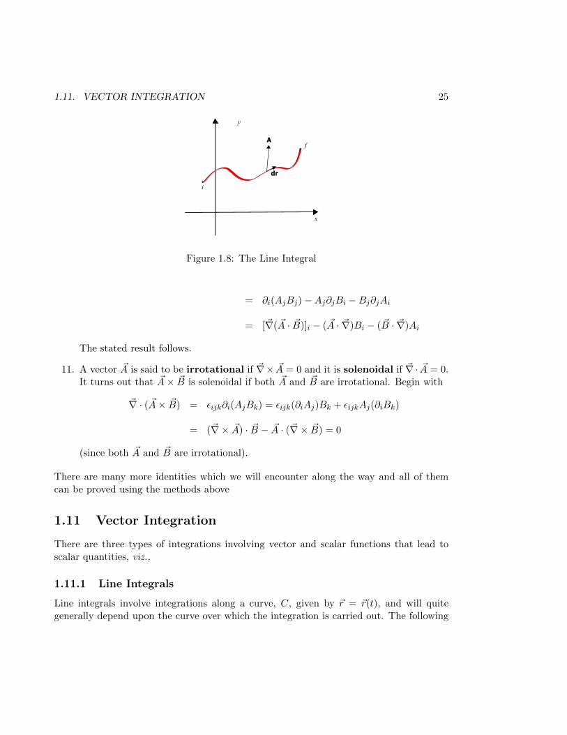
Figure 1.8: The Line Integral
= ∂i(AjBj)−Aj∂jBi −Bj∂jAi
= [~∇( ~A · ~B)]i − ( ~A · ~∇)Bi − ( ~B · ~∇)Ai
The stated result follows.
11. A vector ~A is said to be irrotational if ~∇× ~A = 0 and it is solenoidal if ~∇· ~A = 0.It turns out that ~A× ~B is solenoidal if both ~A and ~B are irrotational. Begin with
~∇ · ( ~A× ~B) = εijk∂i(AjBk) = εijk(∂iAj)Bk + εijkAj(∂iBk)
= (~∇× ~A) · ~B − ~A · (~∇× ~B) = 0
(since both ~A and ~B are irrotational).
There are many more identities which we will encounter along the way and all of themcan be proved using the methods above
1.11 Vector Integration
There are three types of integrations involving vector and scalar functions that lead toscalar quantities, viz.,
1.11.1 Line Integrals
Line integrals involve integrations along a curve, C, given by ~r = ~r(t), and will quitegenerally depend upon the curve over which the integration is carried out. The following
26 CHAPTER 1. VECTORS
are basic possibilities:
∫ f
i,Cφ(~r)ds,
∫ f
i,C
~A(~r)ds,
∫ f
i,Cφ(~r)d~r,
∫ f
i,C
~A(~r)× d~r,∫ f
i,C
~A(~r) · d~r, (1.11.1)
where ds = |~v|dt represents the length of an infinitesimal line element on C and d~r = ~vdtis an infinitesimal displacement along (tangent to) C. Each integral may be defined inthe usual way, as the limit of an infinite (Riemann) sum. The first and last integrals yieldscalars, the others are vectors. The curve may be open or closed and i and f are thebeginning and endpoints of the integration.
If φ(~r) represents the density of a “wire” laid along C, then the first integral returnsthe mass of the wire. On the other hand, a well-known example of the last line integral isthe work performed by a force ~F in moving a particle along some trajectory, C (see figure(1.8). A particularly interesting case occurs when the vector ~A is the gradient of a scalarfunction, i.e., ~A = ~∇φ. In this case,
∫ f
i,C
~A · d~r =
∫ f
i,C
~∇φ · d~r =
∫ f
i,Cdφ = φ(~rf )− φ(~ri) (1.11.2)
showing that the integral depends only on the endpoints and not on the curve C itself. Avector whose line integral is independent of the path along which the integration is carriedout is called conservative. Every conservative vector then obeys∮
C
~A · d~r = 0, (1.11.3)
for every closed path. Conversely, any vector that obeys (1.11.3) is expressible as thegradient of a scalar function, for∮
C
~A · d~r = 0⇒ ~A · d~r = dφ = ~∇φ · d~r (1.11.4)
and, since d~r is arbitrary, it follows that ~A = ~∇φ.
One does not need to evaluate its line integral to determine whether or not a vectoris conservative. From the fact that the curl of a gradient vanishes it follows that if ~A isconservative then ~∇ × ~A = 0. The converse is also true, since if ~A is irrotational thenεijk∂jAk = 0 for all i. These are simply integrability conditions for a function φ defined byAk = ∂kφ, therefore every irrotational vector is conservative and vice versa. The function−φ is generally called a potential of ~A.
1.12. INTEGRAL THEOREMS 27
n
Figure 1.9: The Surface Integral
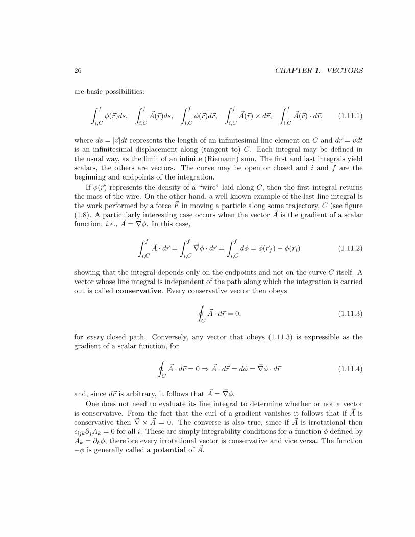
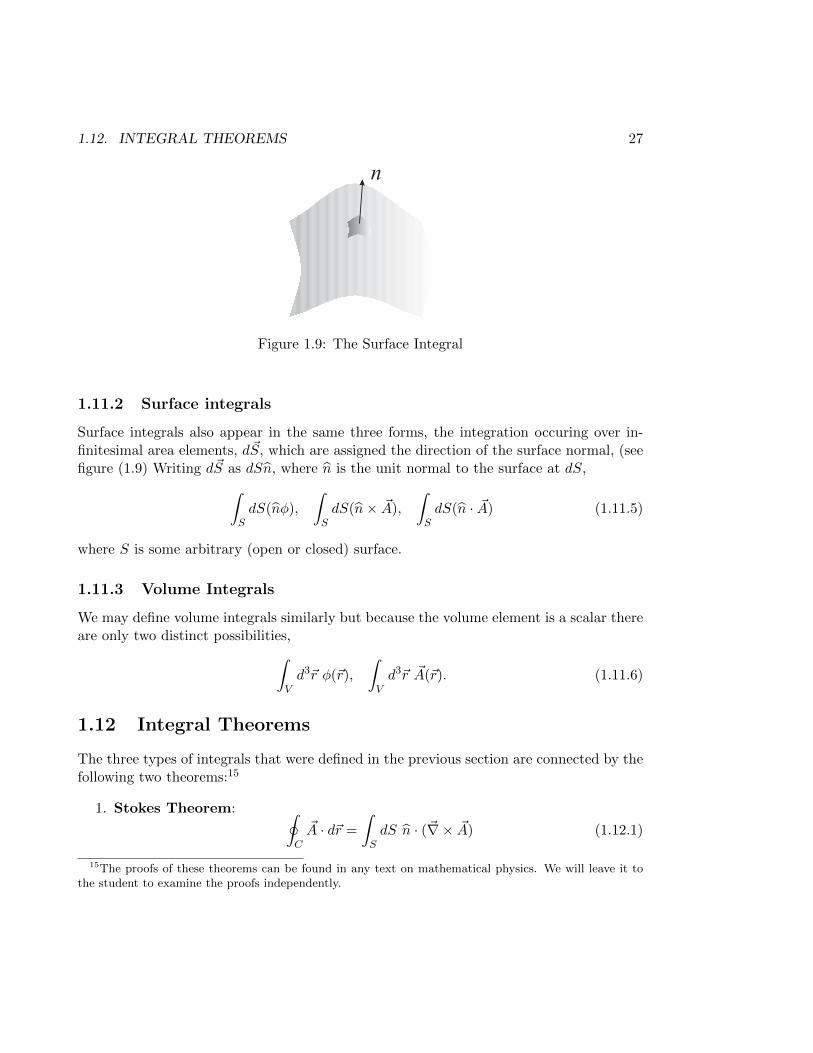
1.11.2 Surface integrals
Surface integrals also appear in the same three forms, the integration occuring over in-finitesimal area elements, d~S, which are assigned the direction of the surface normal, (seefigure (1.9) Writing d~S as dSn, where n is the unit normal to the surface at dS,∫
SdS(nφ),
∫SdS(n× ~A),
∫SdS(n · ~A) (1.11.5)
where S is some arbitrary (open or closed) surface.
1.11.3 Volume Integrals
We may define volume integrals similarly but because the volume element is a scalar thereare only two distinct possibilities,∫
Vd3~r φ(~r),
∫Vd3~r ~A(~r). (1.11.6)
1.12 Integral Theorems
The three types of integrals that were defined in the previous section are connected by thefollowing two theorems:15
1. Stokes Theorem: ∮C
~A · d~r =
∫SdS n · (~∇× ~A) (1.12.1)
15The proofs of these theorems can be found in any text on mathematical physics. We will leave it tothe student to examine the proofs independently.
28 CHAPTER 1. VECTORS
where C is a closed curve, S is a surface bounded by C, and n is normal to thesurface element dS, chosen to obey the right hand rule, i.e., if the fingers of theright hand point in the direction of d~r along the curve then the outstretched thumbdetermines the choice of the orientation of n.
2. Gauss’ theorem: ∮SdS n · ~A =
∫Vd3~r ~∇ · ~A (1.12.2)
where S is a closed surface, n is the outward directed normal to S and V is thevolume bounded S.
While we accept these theorems without proof here, we shall now use then to prove somecorollaries that will turn out to be useful in the future.
1.12.1 Corollaries of Stokes’ Theorem
We will prove the following three relations:
1.∮C φd~r =
∫S dS(n× ~∇φ)
2.∮C d~r × ~A =
∫S dS(n× ~∇)× ~A
where C is a closed curve and S is the surface bounded by C in each case.The proofs are quite simple. Define the vector ~A = ~aφ, where ~a is an arbitrary,
constant vector then by Stokes’ theorem,∮C
~A · d~r = ~a ·∮φd~r =
∫SdSn · (~∇× ~aφ) =
∫SdSn · (~∇φ× ~a)
= ~a ·∫SdS(n× ~∇φ) (1.12.3)
Thus
~a ·(∮
φd~r −∫SdS(n× ~∇φ)
)= 0 (1.12.4)
holds for arbitrary vectors implying the first identity.The second identity may be derived similarly, by using ~B = ~a× ~A in Stokes’ theorem.
Then ∮C
~B · d~r =
∮C~a× ~A · d~r = −
∮C
(d~r ×A) · ~a
=
∫SdS n · (~∇× ~B) =
∫SdS [(n× ~∇) · ~B]
1.12. INTEGRAL THEOREMS 29
=
∫SdS [(n× ~∇) · (~a× ~A)] (1.12.5)
But it is easy to show that16 (n× ~∇) · (~a× ~A) = −[(n× ~∇)× ~A] · ~a, therefore
~a ·[∮
C(d~r ×A)−
∫SdS[n× (~∇× ~A)]
]= 0 (1.12.6)
Again ~a was arbitrary, therefore the second identity follows.
1.12.2 Corollaries of Gauss’ theorem
We will prove three relations that will be quite helpful to us in the future, viz.,
1.∮S dS( ~A× n) =
∫V d
3~r ~∇× ~A
2. If φ and ψ are two arbitrary functions, then
(a) Green’s first identity:∫Vd3~r [~∇φ · ~∇ψ + φ~∇2ψ] =
∫SdS n · φ~∇ψ (1.12.7)
and
(b) Green’s second identity:∫Vd3~r [φ~∇2ψ − ψ~∇2φ] =
∫SdS n · [φ~∇ψ − ψ~∇φ] (1.12.8)
To prove the first corollary we will employ the trick we used to prove the corollaries ofStoke’s theorem. For a constant vector ~a, let ~B = ~a× ~A and apply Gauss’ law∮
SdS(n · ~B) =
∫Vd3~r ~∇ · ~B ⇒
∮SdS[n · (~a× ~A)] =
∫d3~r ~∇ · (~a× ~A) (1.12.9)
Developing the last relation, using some of the vector identities we proved earlier, we find
~a ·[∮
SdS(n× ~A)−
∫Vd3~r ~∇× ~A
]= 0 (1.12.10)
But since ~a is arbitrary, the identity follows.To prove Green’s two theorems is equally straightforward. Take ~A = φ~∇ψ and apply
Gauss’ theorem. Since
~∇ · ~A = ~∇ · (φ~∇ψ) = (~∇φ) · (~∇ψ) + φ~∇2ψ, (1.12.11)
16Problem: Use the properties of the Levi-Civita tensor to show this
30 CHAPTER 1. VECTORS
it follows that the first of Green’s theorems is just Gauss’ theorem,∫Vd3~r [~∇φ · ~∇ψ + φ~∇2ψ] =
∫SdS n · φ~∇ψ (1.12.12)
To prove the second identity, consider ~B = ψ~∇φ and again apply Gauss’ theorem to get∫Vd3~r [~∇ψ · ~∇φ+ ψ~∇2φ] =
∫SdS n · ψ~∇φ (1.12.13)
Subtracting the second from the first gives∫Vd3~r [φ~∇2ψ − ψ~∇2φ] =
∫SdS n · [φ~∇ψ − ψ~∇φ] (1.12.14)
which is Green’s second identity.This chapter does not do justice to the vast area of vector analysis. On the contrary,
most proofs have not been given and many useful identities have been neglected. Whathas been presented is only an introduction to the material we will immediately need.Consequently, as we progress, expect to periodically encounter detours in which furthervector analysis will be presented, often as exercises in the footnotes.
Chapter 2
Newton’s Laws and SimpleApplications
2.1 Introduction
Theoretical mechanics is concerned with the temporal “evolution” of a physical system,be it a single particle or a complex system of particles that interact among themselves.By “evolution” one simply means a continuous change in “configuration”, i.e., a changein some set of parameters that define the system. The fundamental problem is thereforetwo-fold: on the one hand it is necessary to determine the appropriate parameters thatcompletely define a system within the limits of experimental possibility (disregarding lim-itations imposed by current technology) and on the other it is necessary to determine theequations (the dynamical equations) that govern the evolution of these parameters.
Most realistic physical systems encountered in daily life are complex. Nevertheless wetake a point of view, expressed by the Greeks as early as the third century before Christand later reiterated by Newton, that every complex system can be decomposed into andsubsequently reconstructed from elementary constituents which we will call “particles”.In its most idealized form a particle is merely a mathematical point endowed with somephysical charateristics, which could be for example a “mass”, a “charge” etc., but withno discernible geometric structure. These are the so-called “elementary particles”. Theconcept is also useful as an approximation, if the volume of the object we are studyingis very small compared to typical volumes over which its evolution occurs. Thus to areasonable approximation, for example, the earth could be considered a particle if weare interested in its motion about the sun, but it is certainly not a particle if we areinterested in its revolution about its North-South axis or in events that occur upon it.Galaxies are particles compared with typical distances over which they may freely evolvebut certainly not particles if we are interested in their structural properties. On the other
31
32 CHAPTER 2. NEWTON’S LAWS AND SIMPLE APPLICATIONS
x
y
z t
nb
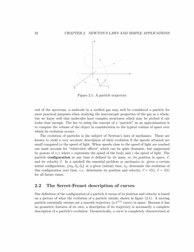
Figure 2.1: A particle trajectory
end of the spectrum, a molecule in a rarified gas may well be considered a particle formost practical purposes when studying the macroscopic properties of the gas as a whole,but we know well that molecules have complex structures which may be probed if onelooks close enough. The key to using the concept of a “particle” as an approximation isto compare the volume of the object in consideration to the typical volume of space overwhich its evolution occurs.
The evolution of particles is the subject of Newton’s laws of mechanics. These areknown to yield a very accurate description of their evolution if the speeds attained aresmall compared to the speed of light. When speeds close to the speed of light are reachedone must account for “relativistic effects” which can be quite dramatic, but suppressedby powers of v/c where v represents the speed of the body and c the speed of light. Theparticle configuration at any time is defined by its mass, m, its position in space, ~r,and its velocity ~v. In a nutshell the essential problem or mechanics is: given a certaininitial configuration, m0, ~r0, ~v0 at a given (initial) time, t0, determine the evolution ofthis configuration over time, i.e., deterimine its position and velocity, ~r = ~r(t), ~v = ~v(t)for all future times.
2.2 The Serret-Frenet description of curves
Our definition of the configuration of a particle it terms of its position and velocity is basedon a picture of what the evolution of a particle entails, shown in figure (2.1). A movingparticle essentially sweeps out a smooth trajectory (a C(1) curve) in space. Because it hasno geometric features of its own, a description of its trajectory is necessarily a completedescription of a particle’s evolution. Geometrically, a curve is completely characterized at
2.2. THE SERRET-FRENET DESCRIPTION OF CURVES 33
every point by three unit vectors, viz., the tangent, the normal and the bi-normal, andtwo scalars, the curvature and torsion, as we now describe. Let C : ~r(t) represent a curvein space and let s(t) be an invertible function representing the distance along the curve ofthe point given by ~r(t) from some fixed point on the curve. We define the unit tangentvector to the curve ~r = ~r t(s) as
t =d~r
ds(2.2.1)
That t is a unit vector follows from the definition of the path length s,
ds =√dx2 + dy2 + dz2 = |d~r| ⇒ 1 =
∣∣∣∣d~rds∣∣∣∣ (2.2.2)
We also define the unit normal vector to the curve by
dt
ds= κ(s)n (2.2.3)
where κ(s) is a function of position, called the curvature of C. The unit normal n isperpendicular to t because t is a unit vector
t2 = 1⇒ t · dtds
= 0 = κ(s)t · n (2.2.4)
provided that κ(s) 6= 0. The plane spanned by t and n at any point, P , on the curve iscalled the osculating plane of the curve at P and a circle lying in the osculating plane atP , that touches P , has the same tangent at P as the curve itself and radius equal to thereciprocal of the curvature is called the osculating circle at P .
If we define the unit binormal vector as
b = t× n (2.2.5)
then b is clearly perpendicular to both t and n. In this way, t, n, b form a right handedtriad called the Frenet vectors. Together they form a basis for three dimensional space,defining a non-static reference frame called the Frenet frame. Now since b is a unitvector it follows that db/ds is perpendicular to b because
b2 = 0⇒ b · dbds
= 0. (2.2.6)
Moreover, because b · t = 0,
db
ds· t+ b · dt
ds=db
ds· t+ κ(s)b · n =
db
ds· t = 0 (2.2.7)
34 CHAPTER 2. NEWTON’S LAWS AND SIMPLE APPLICATIONS
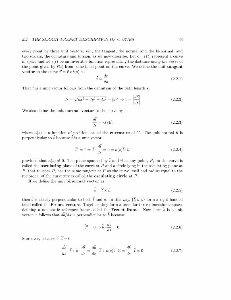
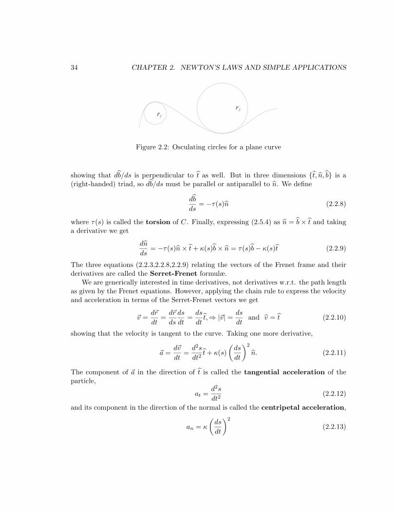
r1
r2
Figure 2.2: Osculating circles for a plane curve
showing that db/ds is perpendicular to t as well. But in three dimensions t, n, b is a(right-handed) triad, so db/ds must be parallel or antiparallel to n. We define
db
ds= −τ(s)n (2.2.8)
where τ(s) is called the torsion of C. Finally, expressing (2.5.4) as n = b× t and takinga derivative we get
dn
ds= −τ(s)n× t+ κ(s)b× n = τ(s)b− κ(s)t (2.2.9)
The three equations (2.2.3,2.2.8,2.2.9) relating the vectors of the Frenet frame and theirderivatives are called the Serret-Frenet formulæ.
We are generically interested in time derivatives, not derivatives w.r.t. the path lengthas given by the Frenet equations. However, applying the chain rule to express the velocityand acceleration in terms of the Serret-Frenet vectors we get
~v =d~r
dt=d~r
ds
ds
dt=ds
dtt,⇒ |~v| = ds
dtand v = t (2.2.10)
showing that the velocity is tangent to the curve. Taking one more derivative,
~a =d~v
dt=d2s
dt2t+ κ(s)
(ds
dt
)2
n. (2.2.11)
The component of ~a in the direction of t is called the tangential acceleration of theparticle,
at =d2s
dt2(2.2.12)
and its component in the direction of the normal is called the centripetal acceleration,
an = κ
(ds
dt
)2
(2.2.13)
2.3. GALILEAN TRANSFORMATIONS 35
Think, for example, of a body performing uniform motion in a circle of radius r.1 Thecurvature of a circle of radius r is 1/r so the centripetal acceleration is v2/r, an expressionthat is already quite familiar. However, we now see that the formula for the centripetalacceleration is quite general, if one thinks of r as the instantaneous radius of curvature asshown pictorially in figure (2.2).
2.3 Galilean Transformations
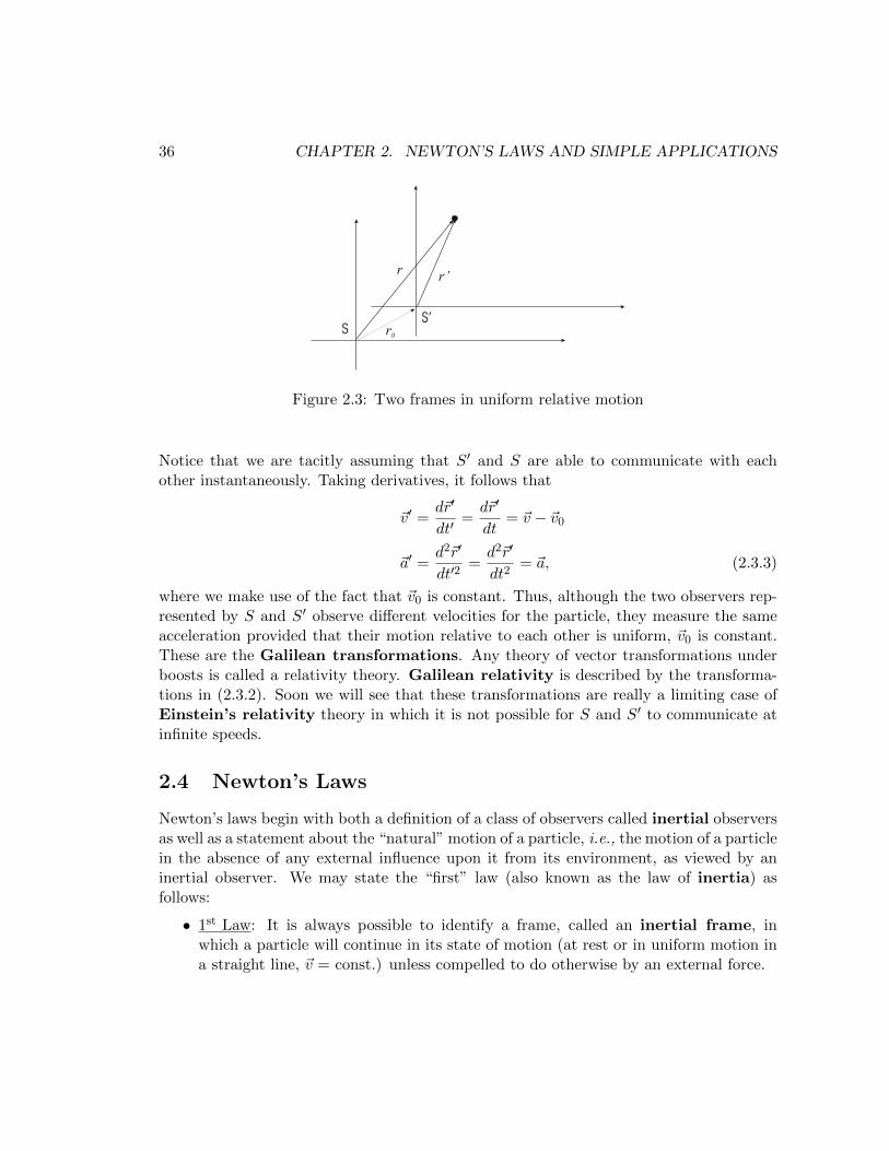
We have already seen how vectors in general and position vectors in particular transformunder rotations of the coordinate system. We may also ask how they transform underboosts, i.e., uniform relative motions between coordinate systems. Therefore considertwo coordinate systems, S and S′ which are such that S′ has a constant velocity ~v0
relative to S. Let P be a point in space (the position of some particle at time t, say) thatis represented in the coordinate system S by the position vector ~r and in the system S′ bythe position vector ~r′. Suppose for convenience (and without loss of generality) that theorigin of the two frames coincide at t = 0. If we let ~r0 represent the position of the originof S′ relative to the S at time t 6= 0, then we could relate the vectors ~r and ~r′ accordingto [see figure (2.3)]
~r = ~r′ + ~r0 = ~r′ + ~v0t (2.3.1)
If we also assume that time is absolute, i.e., that any time interval between two events asmeasured in one frame is identical to the corresponding interval measured in the other,then the two descriptions of the motion of the particle at P are related by
t′ = t
~r′ = ~r − ~v0t (2.3.2)
1 Problem: Consider a helix defined by the curve
~r(t) = (a cosωt, a sinωt, vt)
where a, ω and v are constants, and determine the tangent, normal and binormal vectors, t, n and b.Verify the Serret-Frenet relations and show that the curvature and torsion are constants given by
κ =aω2
a2ω2 + v2
τ =vω
a2ω2 + v2
Notice that if v = 0, so that the curve is a circle (in the x − y plane), then the curvature is just thereciprocal of its radius and the torsion vanishes.
36 CHAPTER 2. NEWTON’S LAWS AND SIMPLE APPLICATIONS
SS’
rr’
r0
Figure 2.3: Two frames in uniform relative motion
Notice that we are tacitly assuming that S′ and S are able to communicate with eachother instantaneously. Taking derivatives, it follows that
~v′ =d~r′
dt′=d~r′
dt= ~v − ~v0
~a′ =d2~r′
dt′2=d2~r′
dt2= ~a, (2.3.3)
where we make use of the fact that ~v0 is constant. Thus, although the two observers rep-resented by S and S′ observe different velocities for the particle, they measure the sameacceleration provided that their motion relative to each other is uniform, ~v0 is constant.These are the Galilean transformations. Any theory of vector transformations underboosts is called a relativity theory. Galilean relativity is described by the transforma-tions in (2.3.2). Soon we will see that these transformations are really a limiting case ofEinstein’s relativity theory in which it is not possible for S and S′ to communicate atinfinite speeds.
2.4 Newton’s Laws
Newton’s laws begin with both a definition of a class of observers called inertial observersas well as a statement about the “natural” motion of a particle, i.e., the motion of a particlein the absence of any external influence upon it from its environment, as viewed by aninertial observer. We may state the “first” law (also known as the law of inertia) asfollows:
• 1st Law: It is always possible to identify a frame, called an inertial frame, inwhich a particle will continue in its state of motion (at rest or in uniform motion ina straight line, ~v = const.) unless compelled to do otherwise by an external force.
2.4. NEWTON’S LAWS 37
In the absence of any external force, the inertial observer can mathematically describe theparticle’s motion by the statement d~v/dt = 0. It is important to note that there is notenough content in the law for the observer to simultaneously determine both if (s)he isinertial and if the particle being observed is “free”. Only when one fact is known can theother be determined. If the observer knows herself to be inertial then a particle is free ifand only if it moves with a constant velocity relative to her and, conversely, if the particleis known to be free then she is inertial if and only if the particle’s velocity relative to heris constant.2
If m is the particle mass, which we assume constant, we may introduce the momentum,~p = m~v, and restate the first law in terms of it as follows: from the point of view of aninertial observer
d~v
dt= 0 = m
d~v
dt⇒ d~p
dt= 0. (2.4.1)
Newton goes on to say that any deviation from this “free” behavior is attributable to thepresence of an external force,
• 2nd Law: Viewed from an inertial frame, the rate of change of momentum is equalto the external, applied “force”
d~p
dt= ~F ext(~r,~v, t) (2.4.2)
Notice that because ~p is a vector, so is ~F ext. This law is a definition of the term “externalforce” and does not specify it. ~F ext must be determined by experiment. Once ~F ext isknown by careful experimentation, then (2.4.2), viewed as a differential equation, gives theparticle trajectory subject, as always, to some initial conditions. Every effort is thereforedirected to determining the “force law”, i.e., the form of ~F ext. Note that “force” hasmechanical dimension [F ] = ml/t2. In the MKS system, force is measured in “Newtons”and in the CGS system it is measured in “dynes”. As examples we know of
1. Hooke’s Law: The force exerted by a spring, stretched by a distance |~r|,
~F = −k~r,
where ~r represents a displacement along the length of the spring from some positionat which the spring is in equilibrium, and k is a constant whose mechanical dimensionis [k] = m/t2 or N/m (MKS) and dynes/cm (CGS).
2 The inertial observer in Newtonian mechanics is therefore a primitive concept. Newton asserts thatsuch frames exist, but does not state independently how they are determined (Newton considered observers“moving at a constant velocity relative to the fixed stars” as inertial). The existence of inertial framesis also asserted in Einstein’s special theory of relativity without further elaboration, but in the generaltheory inertial frames may exist only locally, i.e., over infinitesimal regions of space-time.
38 CHAPTER 2. NEWTON’S LAWS AND SIMPLE APPLICATIONS
2. Newton’s law of Gravity: The gravitational force exerted by a point-like mass m1 onanother point-like mass m2
~F1→2 = −Gm1m2
r2r,
where r is the separation between two particles, r is the unit vector that pointsfrom the particle labeled 1 to the particle labeled 2 and G is “Newtons constant ofuniversal gravitation”, with mechanical dimension [G] = l3/mt2 or N·m2/kg2 (MKS)and dyne·cm/g2. in the CGS system.
3. Coulomb’s law: The electrostatic force exerted by a point-like charge q1 on anotherpoint-like charge q2
~F1→2 =1
4πεo
q1q2
r2r,
where r is the separation between the charges, r points from the charge labeled 1 tothe charge labeled 2 and C = 1/4πε0 is “Coulomb’s constant” written in terms ofthe electric permitivity of the vacuum ε0. The electric permitivity has mechanicaldimension [ε0] =Coulomb2/N · m2 (MKS).
4. Frictional Drag: The “drag” or resistance offered by a medium to the motion of abody (whose dimensions are much larger than the typical dimensions of the moleculesof the medium) inside it,
~Fdrag = −k|~v|αv,
where k and α are constants, the first representing the strength of the drag andthe second its dependence on the velocity, ~v of the body. The exponent α canhave no mechanical dimension, but the mechanical dimension of k depends on α:[k] =N·sα/mα. This expression for the drag is valid so long as the speed of the bodyis not comparable to the speed of sound, c, in the medium. If the |~v| c then theindex α is on the order of unity. α gets larger as the speed of sound is approached,which makes air drag significant at high speeds. The constant k depends on theviscosity of the medium and the geometry of the body.
While the first law can be seen as an positing the existence of the inertial frame anddefining it by specifying what is the “natural” motion of a particle observed from such aframe in the absence of any external influence, and the second defines quantitatively theconcept of an external influence (or force), the third law of Newton is actually a law in itsclassical sense:
• 3rd Law: To every action of (force applied by) one particle on another, there is anequal and contrary reaction of the other on the first, i.e.,
~F1→2 = −~F2→1 (2.4.3)
2.5. NEWTON’S LAWS AND THE SERRET FRENET FORMULÆ 39
This law does not have general applicability and neither does it have an obviousgeneralization. It is true only when
– the forces between the particles act along the line joining the particles,
– the forces do not depend on the velocities of the particles themselves, and
– all velocities involved are small compared with the speed of light.
It does not, for example, hold for the Lorentz force of electrodynamics.
2.5 Newton’s Laws and the Serret Frenet Formulæ
Newton’s description of particle dynamics can be neatly connected with the Serret-Frenetdescription of curves. In general,
~v =ds
dtt
~a =d~v
dt=d2s
dt2t+ κ(t)
(ds
dt
)2
n (2.5.1)
and so
t = v,ds
dt= |~v| and
d2s
dt2= v · ~a (2.5.2)
It also follows that
~v × ~a = κ|~v|3 b ⇒ κ =|~v × ~a||~v|3
(2.5.3)
and the binormal vector is
b =~v × ~a|~v × ~a|
, (2.5.4)
therefore using the fact that t, n, b form a right handed triad we find the normal vector,
n =(~v × ~a)× v|~v × ~a|
. (2.5.5)
Let us compute the torsion from
db
ds= −τ n ⇒ τ = − n
|~v|· dbdt, (2.5.6)
where b is given in (2.5.4). Then,3
τ = − n
|~v|· ddt
[~v × ~a|~v × ~a|
]3Problem: Show that
d
dt
1
|~v × ~a| = − 1
|~v × ~a|3 [~v × (~v × ~a) · ~a]
40 CHAPTER 2. NEWTON’S LAWS AND SIMPLE APPLICATIONS
= − n
|~v|·
[~v × ~a|~v × ~a|
− ~v × ~a|~v × ~a|3
[~v × (~v × ~a) · ~a]
](2.5.7)
and, since n is perpendicular to ~v × ~a, it follows that
τ = − n
|~v|· ~v × ~a|~v × ~a|
= − [(~v × ~a)× v] · (~v × ~a)
|~v||~v × ~a|2
= −~a · (~v × ~a)
|~v × ~a|2=~v · (~a× ~a)
κ2|~v|6=
(~v × ~a) · ~aκ2|~v|6
, (2.5.8)
where we used n = (~v × ~a) × v/|~v × ~a| and the symmetries of the triple product. Noticethat the torsion is proportional to the rate of change of the acceleration (called the jerk)and does not vanish only if the jerk has a non-vanishing component perpendicular to theplane containing the velocity and acceleration.
One may re-express everything in terms of the Newtonian force, considering that ~a =~F/m, and we now summarize the relationship between the Serret-Frenet description ofcurves and the Newtonian description of motion:
t = v,ds
dt= |~v|, d2s
dt2=v · ~Fm
n =(~v × ~F )× v|~v × ~F |
b =(~v × ~F )
|~v × ~F |
κ =|~v × ~F |m|~v|3
τ =(~v × ~F ) · ~Fm2κ2|~v|6
(2.5.9)
The force is therefore responsible for generating both the curvature and the torsion.4 Togenerate a curvature ~F must have a component orthogonal to ~v and to generate a torsionthe rate of change of ~F should have a component perpendicular to the plane containing
4Show that
• for a “central force” (eg., Hooke’s law, Newton’s law of gravity, Coulomb’s law), the torsion of theparticle trajectory vanishes, and
• for the frictional drag force, both the curvature and the torsion vanish.
What do these facts mean in each case?
2.6. ONE DIMENSIONAL MOTION 41
~v and ~F . For example, during uniform motion in a circle of radius r the tangentialacceleration is zero, implying that v · ~F = 0 (the force must be perpendicular to thevelocity). The curvature of the circle is just 1/r and the fourth equation tells us that
|~F⊥| =m~v2
r(2.5.10)
which is the well known expression for the (magnitude of the) centripetal force on theparticle. In fact, the above formula holds for the component of ~F perpendicular to thevelocity at all times, even if the motion is not circular and uniform, provided that r istaken to be the instantaneous radius of curvature of the trajectory and ~v the particle’sinstantaneous velocity.
2.6 One dimensional motion
We will now examine some simple applications of Newton’s laws. But first, let us developsome solution methods. In a single spatial dimension, Newton’s second law of motionyields a single equation,
dp
dt= F (t, x, v) (2.6.1)
where the force may depend quite generally on time, the position and the velocity of thebody but not on higher derivatives, such as the acceleration.
• If the force depends only on time, the equation of motion can be easily integratedtwice. Without loss of generality, let the initial time be set to zero, i.e., t0 = 0.This can always be done because it simply amounts to a resetting of our clock. Forconstant m,
mdv
dt= F (t)⇒ m
∫ v
v0
dv =
∫ t
0dt′F (t′)⇒ v − v0 =
∫ t
0dt′F (t′) (2.6.2)
This is the first integral. Noting that v = dx/dt, the equation
dx
dt= v0 +
1
m
∫ t
0dt′F (t′) (2.6.3)
may be integrated again to give
x(t) = x0 + v0t+1
m
∫ t
0dt′∫ t′
0dt′′F (t′′) (2.6.4)
where x0 is the initial position of the particle, which also may be set to zero withoutloss of generality. This would exploit our freedom to choose an origin. If F (t) is a
42 CHAPTER 2. NEWTON’S LAWS AND SIMPLE APPLICATIONS
constant, independent of time, let F = ma. For instance, a = −g could represent theacceleration of a particle in the gravitational field of the earth, close to its surface(g = 9.81 m/s2). Then
x(t) = x0 + v0t+1
2at2 (2.6.5)
which is the well known kinematical formula.
• If the applied force depends only on the position of the particle, as for example theforce exerted by a spring on a body depends only on the displacement of the bodyfrom the equilibrium position of the spring (Hooke’s law), then a useful trick is toconsider the velocity as a function of position, i.e.,
v(t) = v x(t) = v[x(t)] (2.6.6)
and use the chain rule to reexpress the rate of change of momentum as
mdv
dt= m
dv
dx
dx
dt= mv
dv
dx= F (x) (2.6.7)
Integrating this equation once gives
m
∫ v
v0
vdv =
∫ x
0F (x′)dx′ (2.6.8)
(where we have used our freedom to choose an origin by setting x0 = 0). Performingthe integrals gives
1
2m(v2 − v2
0) =
∫ x
0F (x′)dx′ ⇒ v = ±
√v2
0 +2
m
∫ x
0F (x′)dx′ (2.6.9)
and rewriting the velocity as dx/dt,
dx
dt= ±
√v2
0 +2
m
∫ x
0F (x′)dx′ ⇒
∫ x
0
dx′√v2
0 + 2m
∫ x′0 F (x′′)dx′′
= ±∫ t
0dt = ±t.
(2.6.10)If the integral on the left can be performed we obtain t = t(v0, x), which mustbe inverted to obtain x = x(v0, t). Neither of the two steps need be trivial toperform, nevertheless the above constitutes a complete albeit implicit solution in tothe problem.
2.6. ONE DIMENSIONAL MOTION 43
• If the force depends only on the velocity, the second law of motion may also be inte-grated to obtain an implicit solution, provided that the integrations and inversionscan be performed. Consider
mdv
dt= F (v)⇒ m
∫ v
v0
dv′
F (v′)= t (2.6.11)
If the integral can be done, we get t = t(v, v0). If the function can be inverted,we would get v = v(v0, t) which can be integrated once more to obtain the desiredsolution, so
dx
dt= v(v0, t)⇒ x = x0 +
∫ t
0v(v0, t
′)dt′ (2.6.12)
would constitute a complete solution to the problem. It is sometimes convenient tocombine the trick of considering the velocity as a function of position and writing
mvdv
dx= F (v)⇒
∫ v
v0
v′dv′
F (v′)=
x
m(2.6.13)
setting x0 = 0. Assuming the integral can be performed, we obtain v = v(v0, x),which can be integrated once more
dx
dt= v(v0, x)⇒
∫ x
0
dx′
v(v0, x′)= t (2.6.14)
again giving a complete implicit solution to the problem, but in a different form.
• In the general case,
mdv
dt= F (x, v, t) (2.6.15)
the second law must be treated as the second order differential equation
md2x
dt2− F (x,
dx
dt, t) = 0 (2.6.16)
Needless to say, the problem can be non-linear and difficult to solve, although inrare cases a solution may be obtained. We will examine one such example in thefollowing pages.
We will now work out some specific examples to illustrate these procedures in problemswhere all the required steps can be performed and the answer given in closed form. Inthe worst case scenarios, it is usually possible to integrate the equations numerically.Numerical solutions, while not ideal, are unfortunately what one must appeal to in mostrealistic physical situations. Exact (closed form) solutions on the other hand serve ourintuition best and we will concentrate on these for the most part.
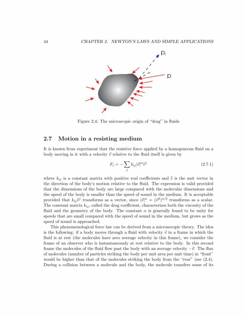
44 CHAPTER 2. NEWTON’S LAWS AND SIMPLE APPLICATIONS
pi
pf
Figure 2.4: The microscopic origin of “drag” in fluids
2.7 Motion in a resisting medium
It is known from experiment that the resistive force applied by a homogeneous fluid on abody moving in it with a velocity ~v relative to the fluid itself is given by
Fi = −∑j
kij |~v|αvj (2.7.1)
where kij is a constant matrix with positive real coefficients and v is the unit vector inthe direction of the body’s motion relative to the fluid. The expression is valid providedthat the dimensions of the body are large compared with the molecular dimensions andthe speed of the body is smaller than the speed of sound in the medium. It is acceptableprovided that kij v
j transforms as a vector, since |~v|α = (~v2)α/2 transforms as a scalar.The constant matrix kij , called the drag coefficient, characterizes both the viscosity of thefluid and the geometry of the body. The constant α is generally found to be unity forspeeds that are small compared with the speed of sound in the medium, but grows as thespeed of sound is approached.
This phenomenological force law can be derived from a microsocopic theory. The ideais the following: if a body moves through a fluid with velocity ~v in a frame in which thefluid is at rest (the molecules have zero average velocity in this frame), we consider theframe of an observer who is instantaneously at rest relative to the body. In this secondframe the molecules of the fluid flow past the body with an average velocity −~v. The fluxof molecules (number of particles striking the body per unit area per unit time) in “front”would be higher than that of the molecules striking the body from the “rear” (see (2.4).During a collision between a molecule and the body, the molecule transfers some of its
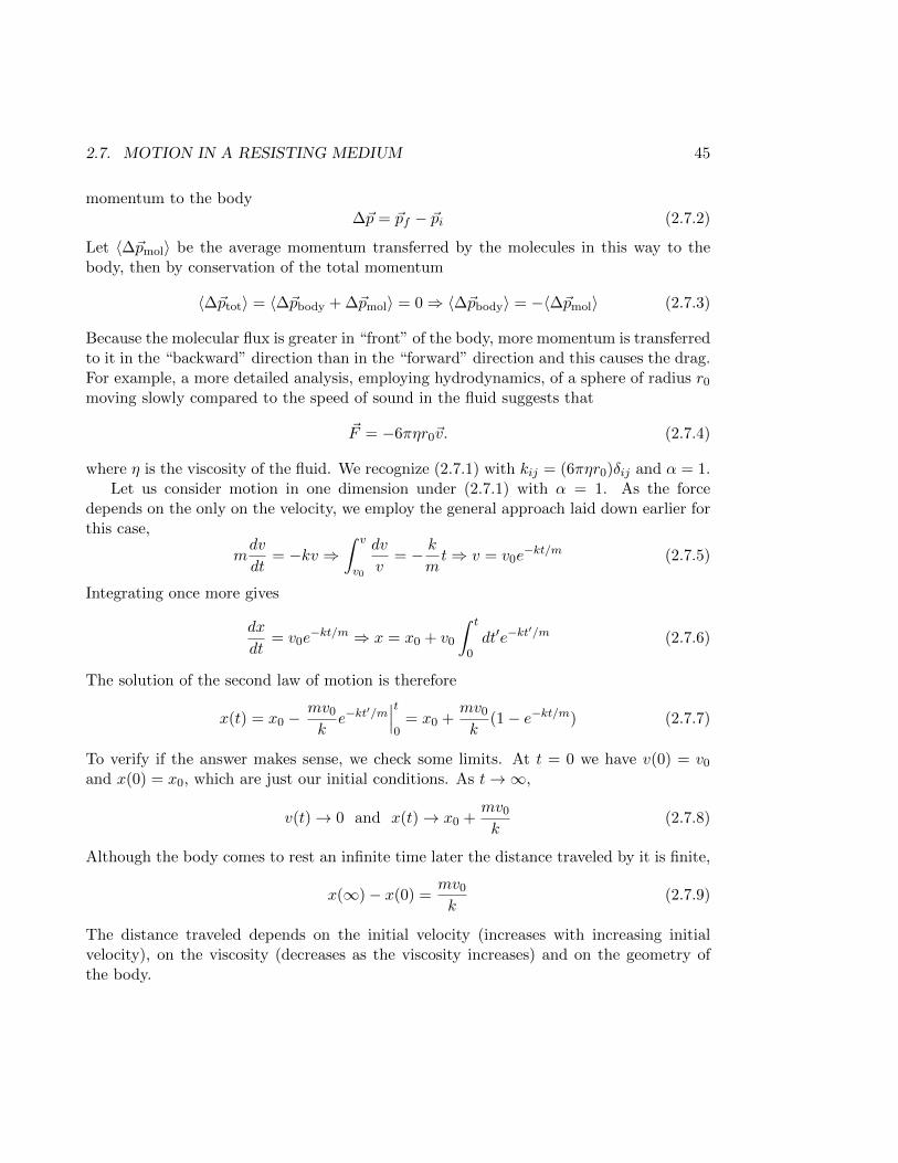
2.7. MOTION IN A RESISTING MEDIUM 45
momentum to the body∆~p = ~pf − ~pi (2.7.2)
Let 〈∆~pmol〉 be the average momentum transferred by the molecules in this way to thebody, then by conservation of the total momentum
〈∆~ptot〉 = 〈∆~pbody + ∆~pmol〉 = 0⇒ 〈∆~pbody〉 = −〈∆~pmol〉 (2.7.3)
Because the molecular flux is greater in “front” of the body, more momentum is transferredto it in the “backward” direction than in the “forward” direction and this causes the drag.For example, a more detailed analysis, employing hydrodynamics, of a sphere of radius r0
moving slowly compared to the speed of sound in the fluid suggests that
~F = −6πηr0~v. (2.7.4)
where η is the viscosity of the fluid. We recognize (2.7.1) with kij = (6πηr0)δij and α = 1.Let us consider motion in one dimension under (2.7.1) with α = 1. As the force
depends on the only on the velocity, we employ the general approach laid down earlier forthis case,
mdv
dt= −kv ⇒
∫ v
v0
dv
v= − k
mt⇒ v = v0e
−kt/m (2.7.5)
Integrating once more gives
dx
dt= v0e
−kt/m ⇒ x = x0 + v0
∫ t
0dt′e−kt
′/m (2.7.6)
The solution of the second law of motion is therefore
x(t) = x0 −mv0
ke−kt
′/m∣∣∣t0
= x0 +mv0
k(1− e−kt/m) (2.7.7)
To verify if the answer makes sense, we check some limits. At t = 0 we have v(0) = v0
and x(0) = x0, which are just our initial conditions. As t→∞,
v(t)→ 0 and x(t)→ x0 +mv0
k(2.7.8)
Although the body comes to rest an infinite time later the distance traveled by it is finite,
x(∞)− x(0) =mv0
k(2.7.9)
The distance traveled depends on the initial velocity (increases with increasing initialvelocity), on the viscosity (decreases as the viscosity increases) and on the geometry ofthe body.
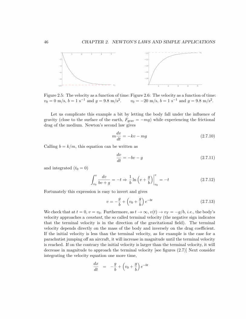
46 CHAPTER 2. NEWTON’S LAWS AND SIMPLE APPLICATIONS
1 2 3 4 5
-10
-8
-6
-4
-2
vT
Figure 2.5: The velocity as a function of time:v0 = 0 m/s, b = 1 s−1 and g = 9.8 m/s2.
1 2 3 4 5
-18
-16
-14
-12
-10 vT
Figure 2.6: The velocity as a function of time:v0 = −20 m/s, b = 1 s−1 and g = 9.8 m/s2.
Let us complicate this example a bit by letting the body fall under the influence ofgravity (close to the surface of the earth, Fgrav = −mg) while experiencing the frictionaldrag of the medium. Newton’s second law gives
mdv
dt= −kv −mg (2.7.10)
Calling b = k/m, this equation can be written as
dv
dt= −bv − g (2.7.11)
and integrated (t0 = 0) ∫ v
v0
dv
bv + g= −t⇒ 1
bln(v +
g
b
)∣∣∣∣vv0
= −t (2.7.12)
Fortunately this expression is easy to invert and gives
v = −gb
+(v0 +
g
b
)e−bt (2.7.13)
We check that at t = 0, v = v0. Furthermore, as t→∞, v(t)→ vT = −g/b, i.e., the body’svelocity approaches a constant, the so called terminal velocity (the negative sign indicatesthat the terminal velocity is in the direction of the gravitational field). The terminalvelocity depends directly on the mass of the body and inversely on the drag coefficient.If the initial velocity is less than the terminal velocity, as for example is the case for aparachutist jumping off an aircraft, it will increase in magnitude until the terminal velocityis reached. If on the contrary the initial velocity is larger than the terminal velocity, it willdecrease in magnitude to approach the terminal velocity [see figures (2.7)] Next considerintegrating the velocity equation one more time,
dx
dt= −g
b+(v0 +
g
b
)e−bt
2.7. MOTION IN A RESISTING MEDIUM 47
⇒ x = x0 −g
bt− 1
b
(v0 +
g
b
)e−bt
∣∣∣∣t0
⇒ x = x0 −g
bt+
1
b
(v0 +
g
b
)(1− e−bt) (2.7.14)
At t = 0, x = x0 as required. As t→∞,
x(t)→ x0 +1
b
(v0 +
g
b
)+ vT t (2.7.15)
This result makes sense because, in the limit of large t, the body moves with constantvelocity equal to its terminal velocity. The effective “initial” position is not the same asx0, but displaced by (v0b+ g)/b2. This essentially accounts for the extra distance traveledwhile the body’s speed was larger than its terminal speed.
2.7.1 Drag and the projectile
We can combine the motions examined above by considering a projectile in the presenceof drag. The equation of motion is now effectively two dimensional,
md~v
dt= −k~v +m~g (2.7.16)
or the (decoupled) set of equations,
dvxdt
= −bvx
dvydt
= −bvy − g (2.7.17)
Suppose that the body has initial velocity
~v0 = v0(cos θ, sin θ) = (v0x, v0y) (2.7.18)
where θ is the angle made with the x−axis, then applying our solutions,
x(t) =v0x
b
(1− e−bt
)y(t) = vT t+
(bv0y + g
b2
)(1− e−bt) (2.7.19)
This trajectory is shown in figure (2.7.1). Notice that it is no longer symmetric about themaximum. This is because the equations do not describe a parabola, as they do when
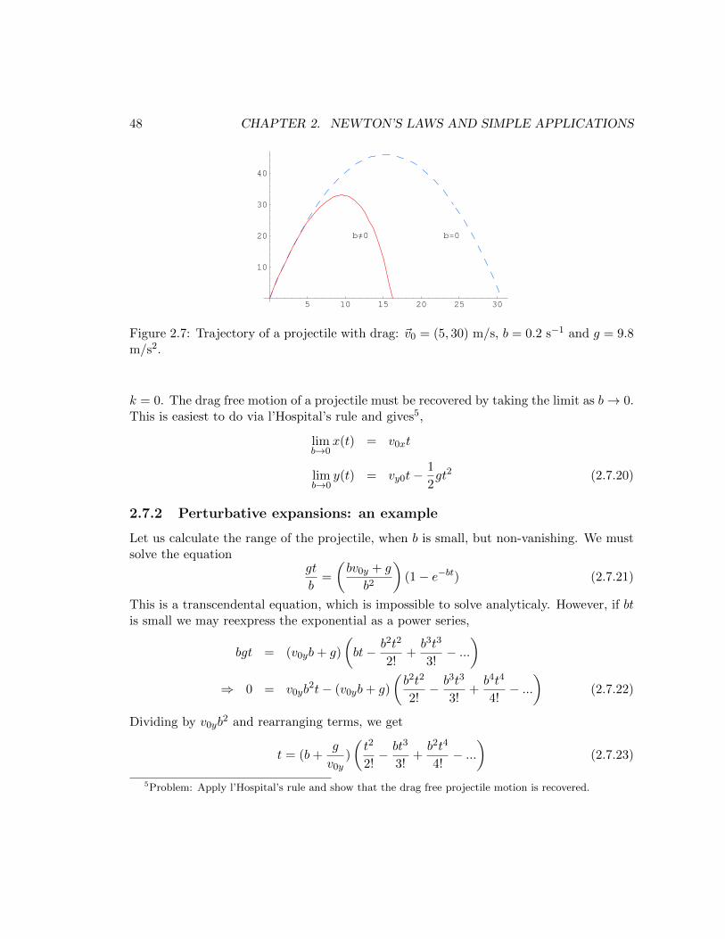
48 CHAPTER 2. NEWTON’S LAWS AND SIMPLE APPLICATIONS
5 10 15 20 25 30
10
20
30
40
b=0b¹0
Figure 2.7: Trajectory of a projectile with drag: ~v0 = (5, 30) m/s, b = 0.2 s−1 and g = 9.8m/s2.
k = 0. The drag free motion of a projectile must be recovered by taking the limit as b→ 0.This is easiest to do via l’Hospital’s rule and gives5,
limb→0
x(t) = v0xt
limb→0
y(t) = vy0t−1
2gt2 (2.7.20)
2.7.2 Perturbative expansions: an example
Let us calculate the range of the projectile, when b is small, but non-vanishing. We mustsolve the equation
gt
b=
(bv0y + g
b2
)(1− e−bt) (2.7.21)
This is a transcendental equation, which is impossible to solve analyticaly. However, if btis small we may reexpress the exponential as a power series,
bgt = (v0yb+ g)
(bt− b2t2
2!+b3t3
3!− ...
)⇒ 0 = v0yb
2t− (v0yb+ g)
(b2t2
2!− b3t3
3!+b4t4
4!− ...
)(2.7.22)
Dividing by v0yb2 and rearranging terms, we get
t = (b+g
v0y)
(t2
2!− bt3
3!+b2t4
4!− ...
)(2.7.23)
5Problem: Apply l’Hospital’s rule and show that the drag free projectile motion is recovered.
2.7. MOTION IN A RESISTING MEDIUM 49
and we want to solve this for t. We now apply a method called “perturbation theory” tosolve this equation. The idea is to expand the solution (2.7.19) about its solution in theabsence of drag, which of course is only meaningful if the effects of drag are “small”. Tomake precise what we mean by “small”, we proceed as follows: if t0 represents the solutionof the equation when b = 0, then the parameter
λ = bt0 (2.7.24)
is dimensionless (recall that [b] = t−1). The time scale t0 will depend on the initialconditions. For small enough b (the drag) the dimensionless quantity λ will also be smalland, since λ is dimensionless, its magnitude will be independent of the units used. Anyparameter that is small, time independent and free of mechanical dimensions can serveas a “perturbation” parameter. What this means is that we assume that the solution of(2.7.23) has the form
t = t0 + λt1 + λ2t2 + ... =
∞∑j=0
λjtj (2.7.25)
where t0 solves (2.7.23) with b = 0, i.e.,
t0 =2v0y
g(2.7.26)
Equation (2.7.23) now becomes
t0 + λt1 + λ2t2 + ... =
(λ
t0+
g
v0y
)(1
2(t0 + λt1 + ...)2 − λ
6t0(t0 + λt1 + ...)3 + ....
)=
(λ
t0+
g
v0y
)(t202
+ λt0t1 −λ
6t20 + ...O(λ2)
)(2.7.27)
and we compare terms with the same power of λ to get t1, t2 etc. To zeroeth order in λwe get
t0 =gt202v0y
⇒ t0 = 0 or t0 =2v0y
g(2.7.28)
which is precisely the same solution we had before, when b = 0. To first order
t1 =t02
+gt0t1v0y
− gt206v0y
⇒ t1 = −v0y
3g(2.7.29)
which is the first correction to b = 0 result: to first order in lambda we find
t ≈ t0 + λt1 =2v0y
g−
2bv20y
3g2=
2v0y
g
[1− bv0y
3g
](2.7.30)
50 CHAPTER 2. NEWTON’S LAWS AND SIMPLE APPLICATIONS
One can go on in this way, calculating t2, t3, etc., by comparing higher and higher powersof lambda in (2.7.27) and using the previously obtained values of t0, t1, t2, etc. Note thatthis method is based on the assumption that the series in (2.7.25) converges. This is nolonger true when λ ≥ 1, so we must require that
λ 1⇒ bt0 1⇒ k mg
2v0y(2.7.31)
Thus the validity of the expansion depends on the mass of the body and the y− componentof the initial velocity. The approximation gets better for larger masses and smaller initialvelocities.
It is now straightforward to also approximate the range of the particle. From the firstequation in (2.7.19),
R′ =v0x
b(1− 1 + bt− b2t2
2+ ...)t=t0+λt1+...
= v0x(t− bt2
2+ ...)t=t0+λt1+...
= v0x
(2v0y
g
[1− bv0y
3g
]− b
2
4v20y
g2+O(b2)
)R′ ≈ 2v0xv0y
g
(1− 4
3
bv0y
g+ ...
)(2.7.32)
The first term is the range of the drag free projectile. As we would expect, the range ofthe projectile is diminished by the drag. We find that it is diminished (to first order in b)by6
∆R = R−R′ ≈ 4
3
bv0xv20y
g2(2.7.33)
2.8 Harmonic motion
A deformed spring generally applies a “restorative” force on any body that is attached toit. The restorative force is directed in such a way as to return the spring to its original
6Problem: The maximum height attained by the projectile is given by vy = 0, i.e.,
g
b=(v0y +
g
b
)(1− bt+
b2t2
2− ...
)Expand t as before (t = t0 + λt1 + ...) with λ = bt0, where t0 is the time taken to reach maximum heightwhen b = 0. Calculate the time taken to reach maximum height and then the maximum height attainedby the projectile.
2.8. HARMONIC MOTION 51
size and shape. If, for example, one end of the spring is attached to an (unmovable) walland the other to a body that is free to move, the restorative force will have the effect ofreturning the body to its original position. Restorative forces can occur in a wide varietyof physical situations. For example consider an object floating in a liquid. If the body ispushed deeper into the liquid, we know from experience that it will bounce back, movingup and down until, over a characteristic period of time, it returns to its original position.Under certain conditions that occur frequently enough to be most interesting and thatwe will discuss later, the magnitude of the restorative force will depend linearly on thedisplacement of the body from its equilibrium position. In general,
Fi = −∑j
kijxj (2.8.1)
where kij is a constant, symmetric matrix of positive, real coefficients. This is a generalversion of “Hooke’s Law”.
2.8.1 Harmonic motion in one dimension
Let us consider motion under Hooke’s law in one dimension. As the force depends onlyon the position of the body, we apply the general method developed earlier for this case
md2x
dt2= −kx⇒ d2x
dt2= − k
mx = −ω2x (2.8.2)
Rewriting the equation as
vdv
dx= −ω2x⇒ 1
2(v2 − v2
0) = −1
2ω2x2, (2.8.3)
where we have taken the equilibrium position of the body to be the origin and v0 is thevelocity at x = 0. This gives
v =dx
dt=√v2
0 − ω2x2 ⇒∫ x
0
dx√v2
0 − ω2x2= t− t0, (2.8.4)
(since we have no right to fix the time at which the body is at its equilbrium position, t0remains arbitrary). The integral is easily solved by substitution and we find
x(t) =v0
ωcos(ω[t− t0]) = A cos(ωt− φ0) (2.8.5)
and
v(t) =dx
dt= −ωA sin(ωt− φ0) (2.8.6)
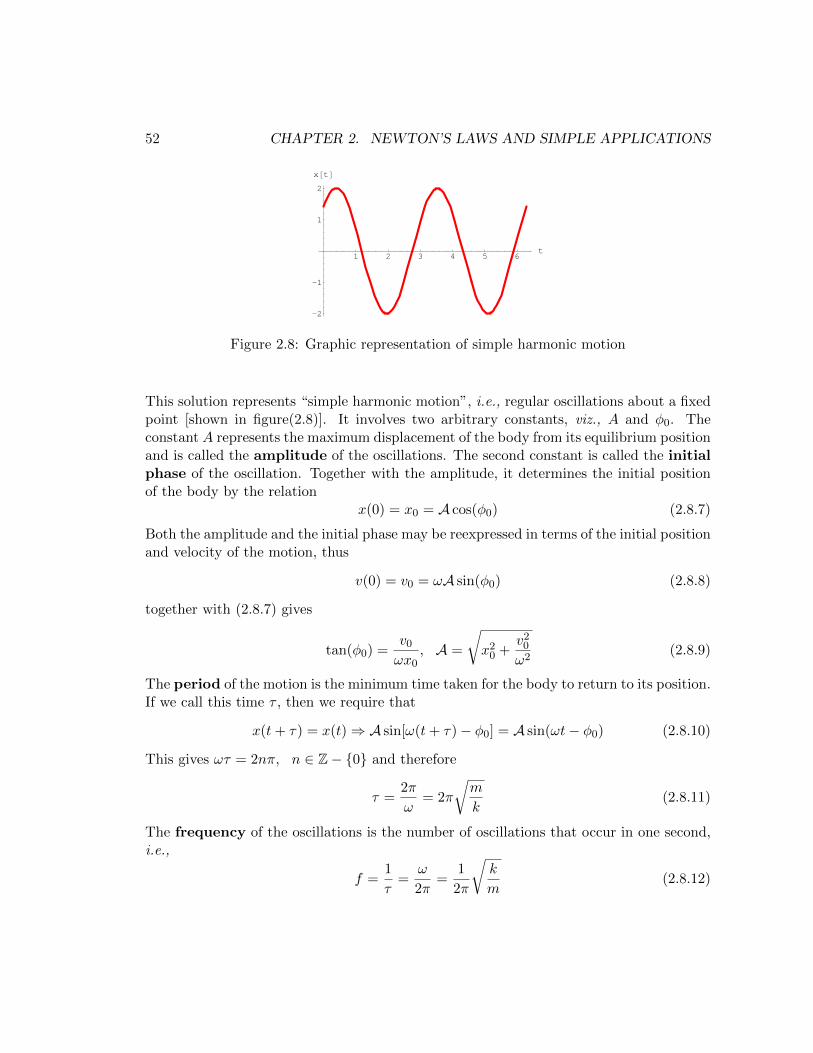
52 CHAPTER 2. NEWTON’S LAWS AND SIMPLE APPLICATIONS
1 2 3 4 5 6t
-2
-1
1
2
x@tD
Figure 2.8: Graphic representation of simple harmonic motion
This solution represents “simple harmonic motion”, i.e., regular oscillations about a fixedpoint [shown in figure(2.8)]. It involves two arbitrary constants, viz., A and φ0. Theconstant A represents the maximum displacement of the body from its equilibrium positionand is called the amplitude of the oscillations. The second constant is called the initialphase of the oscillation. Together with the amplitude, it determines the initial positionof the body by the relation
x(0) = x0 = A cos(φ0) (2.8.7)
Both the amplitude and the initial phase may be reexpressed in terms of the initial positionand velocity of the motion, thus
v(0) = v0 = ωA sin(φ0) (2.8.8)
together with (2.8.7) gives
tan(φ0) =v0
ωx0, A =
√x2
0 +v2
0
ω2(2.8.9)
The period of the motion is the minimum time taken for the body to return to its position.If we call this time τ , then we require that
x(t+ τ) = x(t)⇒ A sin[ω(t+ τ)− φ0] = A sin(ωt− φ0) (2.8.10)
This gives ωτ = 2nπ, n ∈ Z− 0 and therefore
τ =2π
ω= 2π
√m
k(2.8.11)
The frequency of the oscillations is the number of oscillations that occur in one second,i.e.,
f =1
τ=
ω
2π=
1
2π
√k
m(2.8.12)
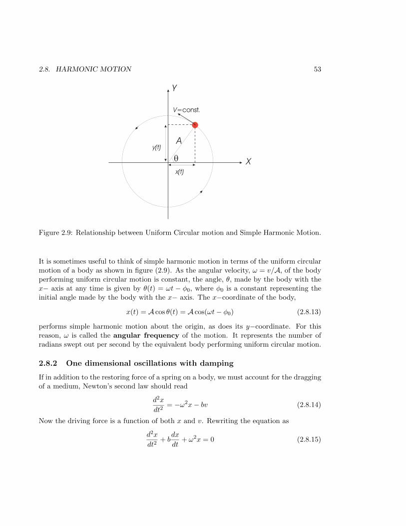
2.8. HARMONIC MOTION 53
x(t)
y(t)
V=const.
X
Y
q
A
Figure 2.9: Relationship between Uniform Circular motion and Simple Harmonic Motion.
It is sometimes useful to think of simple harmonic motion in terms of the uniform circularmotion of a body as shown in figure (2.9). As the angular velocity, ω = v/A, of the bodyperforming uniform circular motion is constant, the angle, θ, made by the body with thex− axis at any time is given by θ(t) = ωt − φ0, where φ0 is a constant representing theinitial angle made by the body with the x− axis. The x−coordinate of the body,
x(t) = A cos θ(t) = A cos(ωt− φ0) (2.8.13)
performs simple harmonic motion about the origin, as does its y−coordinate. For thisreason, ω is called the angular frequency of the motion. It represents the number ofradians swept out per second by the equivalent body performing uniform circular motion.
2.8.2 One dimensional oscillations with damping
If in addition to the restoring force of a spring on a body, we must account for the draggingof a medium, Newton’s second law should read
d2x
dt2= −ω2x− bv (2.8.14)
Now the driving force is a function of both x and v. Rewriting the equation as
d2x
dt2+ b
dx
dt+ ω2x = 0 (2.8.15)
54 CHAPTER 2. NEWTON’S LAWS AND SIMPLE APPLICATIONS
we see that this is a linear, second order differential equation with constant coefficients.To solve this equation, it is best to think of the l.h.s. as the action of the differentialoperator D2 + bD + ω2 on the function x(t), where D = d/dt. Factoring the operator,
(D2 + bD + ω2) = (D − λ+)(D − λ−) (2.8.16)
we find
λ± =−b±
√b2 − 4ω2
2. (2.8.17)
Now because(D − λ+)(D − λ−)x(t) = 0 (2.8.18)
and because the operators (D − λ±) commute, it follows that either
(D − λ+)x(t) = 0 (2.8.19)
or(D − λ−)x(t) = 0. (2.8.20)
Each first order equation is simple to solve, we find
dx±dt− λ±x± = 0⇒ x±(t) = A±e
λ±t (2.8.21)
where A± are arbitrary constants. The general solution of our problem is a linear combi-nation of these two solutions because we are really interested in the second order equationin (2.8.18). Therefore
x(t) = e−bt2
[A+e
√b2
4−ω2t +A−e
−√b2
4−ω2t
](2.8.22)
provided that the eigenvalues are not degenerate, i.e., λ+ 6= λ−. Two cases arise:
• If b2
4 > ω2, the system is said to be overdamped. Calling ω =√
b2
4 − ω2, all
solutions take the form
x(t) = e−bt/2[A+e
ωt +A−e−ωt] (2.8.23)
The motion is not oscillatory, but decays with time to the equilibrium position ofthe body, i.e., x(t → ∞) → 0. The two constants, A±, are determined from theinitial conditions, x(0) = x0 and v(0) = v0. We find7
x0 = A+ +A−
7Problem: Obtain explicit expressions for A± in terms of x0 and v0 from the equations in (2.8.24)
2.8. HARMONIC MOTION 55
v0 = − b2
(A+ +A−) + ω(A+ −A−) (2.8.24)
For real solutions, the coefficients A± must be real. The trajectory is shown as thered curve in figure (2.10).
• If b2
4 < ω2, the system is said to be underdamped. The motion is oscillatory, but
its amplitude decays to zero with time. We could set ω =√ω2 − b2
4 and write
x(t) = e−bt2[A+e
iωt +A−e−iωt] (2.8.25)
Since the position of the body must be real,
x∗(t) = x(t)⇒ A∗+e−iωt +A∗−e
iωt = A+eiωt +A−e
−iωt ⇒ A− = A∗+ (2.8.26)
and thereforex(t) = 2e−bt/2<(A+e
iωt) (2.8.27)
Now A+, being generally complex, can be written as
A+ =A2e−iφ0 (2.8.28)
where A is real and −φ0 is the phase of A+, giving
x(t) = Ae−bt/2<(ei(ωt−φ0)) (2.8.29)
Applying de Moivre’s formula,8 we then find the final form of the solution
x(t) = Ae−bt/2 cos(ωt− φ0) (2.8.30)
This expression is similar to that obtained earlier for the simple harmonic oscillator,except that the amplitude is now decreasing exponentially with time,
A(t) = Ae−bt/2, (2.8.31)
and the frequency of oscillations,
τ =2π
ω=
2π√ω2 − b2
4
⇒ f =
√ω2 − b2
4
2π, (2.8.32)
8De Moivre’s formula readseiθ = cos θ + i sin θ
Show this by expanding the exponential function in a Taylor series about θ = 0 and comparing the realand imaginary parts of the expansion with the Taylor series of the cosine and sine functions respectively.
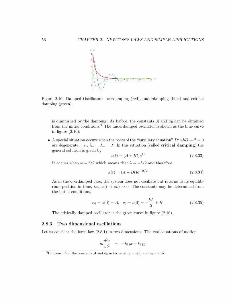
56 CHAPTER 2. NEWTON’S LAWS AND SIMPLE APPLICATIONS
2 4 6 8 10t
-1
1
2
3
4
x@tD
Figure 2.10: Damped Oscillators: overdamping (red), underdamping (blue) and criticaldamping (green).
is diminished by the damping. As before, the constants A and φ0 can be obtainedfrom the initial conditions.9 The underdamped oscillator is shown as the blue curvein figure (2.10).
• A special situation occurs when the roots of the “auxiliary equation”D2+bD+ω2 = 0are degenerate, i.e., λ+ = λ− = λ. In this situation (called critical damping) thegeneral solution is given by
x(t) = (A+Bt)eλt (2.8.33)
It occurs when ω = b/2 which means that λ = −b/2 and therefore
x(t) = (A+Bt)e−bt/2 (2.8.34)
As in the overdamped case, the system does not oscillate but returns to its equilib-rium position in time, i.e., x(t→∞)→ 0. The constants may be determined fromthe initial conditions,
x0 = x(0) = A, v0 = v(0) = −bA2
+B. (2.8.35)
The critically damped oscillator is the green curve in figure (2.10).
2.8.3 Two dimensional oscillations
Let us consider the force law (2.8.1) in two dimensions. The two equations of motion
md2x
dt2= −k11x− k12y
9Problem: Find the constants A and φ0 in terms of x0 = x(0) and v0 = v(0).
2.8. HARMONIC MOTION 57
md2y
dt2= −k21x− k22y (2.8.36)
are coupled, i.e., the motion in any direction is affected by the motion in the other. This isbecause we have not been clever enough to choose a convenient coordinate system i.e., onein which the motions decouple. To see how this can be done, let us rewrite the equationsin matrix form,
md2~r
dt2= −k~r (2.8.37)
where k is the matrix of elements kij . Because k is a constant, symmetric matrix it can
be diagonalized by a constant orthogonal transformation, S. Let the diagonal matrix bekD = SkS−1. Multiplying the equation of motion on the left by S,
md2
dt2(S~r) = −(SkS−1)(S~r) (2.8.38)
where on the left we have used the fact that S is constant and on the right we have insertedunity in the form of S−1S. Calling ~q = S~r, we get
md2~q
dt2= −kD~q. (2.8.39)
But kD is diagonal, so the equation above is just a set of two decoupled harmonic oscillatorswhose characteristic angular frequencies are determined by the eigenvalues of the matrix k.However, the vector ~q represents the position of the body in a rotated coordinate system.Let us suppose that the two eigenvalues of k are k±. Then the equations of motion, interms of ~q = (q+, q−) become
d2q+
dt2= −k+
mq+ = −ω2
+q+
d2q−dt2
= −k−mq− = −ω2
−q− (2.8.40)
which have the solutionsq± = A± cos(ω±t− φ±) (2.8.41)
The constants A± and φ± are related to the initial conditions (four of them because we arein two dimensions; there are two initial conditions per dimension, viz., the initial positionand the initial velocity).
But what are q± and ω±? To answer this question we must first determine S. Beingtwo dimensional and orthogonal it must have the form
S =
(cos η sin η− sin η cos η
)(2.8.42)
58 CHAPTER 2. NEWTON’S LAWS AND SIMPLE APPLICATIONS
and we would like to find η. By simply multiplying out the matrices, we determine thatfor kD to be diagonal
k12 cos 2η − 1
2(k11 − k22) sin 2η = 0⇒ η =
1
2tan−1
[2k12
(k11 − k22)
](2.8.43)
and that the eigenvalues of k are
k± =1
2
[(k11 + k22)±
√(k11 − k22)2 + 4k2
12
]= mω2
± (2.8.44)
These are the “normal modes” of the system and f± = ω±/2π are its “normal frequen-cies”. Moreover, since ~q = S~r we obtain the solution in terms of the old coordinates byinversion,x(t)
y(t)
=
cos η − sin η
sin η cos η
q+
q−
=
cos η − sin η
sin η cos η
A+ cos(ω+t− φ+)
A− cos(ω−t− φ−)
(2.8.45)
We have assumed that the eigenvalues of k are positive, which is true only if k11k22 > k212.
It should be clear that the above procedure can be carried out in any number of dimensions.The diagonalizing matrix will always be a member of special orthogonal group SO(n) andtherefore involve n(n− 1)/2 free parameters (the Euler angles).
The method can also be applied to more complex situations, such as the one thatoccurs in solids. A solid can be thought of as a very large number, N , of molecules each ofwhich oscillates about some equilibrium position. The net force acting upon any moleculeis due to its interaction with all the molecules in its neighborhood and can be quitecomplicated. However, it turns out that Hooke’s law is an excellent approximation undernormal conditions, so (2.8.1) applies. A generalization of the diagonalization illustrated inthe simple two dimensional example above can be applied to reduce the solid to a systemof 3N decoupled harmonic oscillators which, as we have just seen, is easily solved.
2.8.4 Trajectories in the plane
In the present, parametrized form it is difficult to visualize the trajectory of the body inthe x− y plane. For this it is sometimes better to determine the trajectory as an implicitfunction f(x, y) =const. We begin with the simpler situation that occurs when k12 = 0.This gives η = 0, ω2
+ = k11/m and ω2− = k22/m. Therefore
x(t) = A+ cos(ω+t− φ+), y(t) = A− cos(ω−t− φ−), (2.8.46)
If we further specialize to the case when ω+ = ω− = ω, then the motions in the x− andy− directions differ only by amplitude and a phase. If we let δ = φ+ − φ− then
y = A− cos(ωt− φ+ + δ)
2.8. HARMONIC MOTION 59
= A−[cos(ωt− φ+) cos δ − sin(ωt− φ+) sin δ]
=A−A+
[x cos δ −√A2
+ − x2 sin δ] (2.8.47)
Some special cases are particularly interesting:
• When δ = 2nπ, n ∈ Z,
y =A−A+
x (2.8.48)
which is the equation of a straight line in the x− y plane with positive slope deter-mined by the respective amplitudes.
• When δ = (2n+ 1)π, n ∈ Z,
y = −A−A+
x, (2.8.49)
which is the equation of a straight line in the x− y plane with negative slope whosemagnitude is again determined by the respective amplitudes.
• When δ = (2n+ 1)π2 , n ∈ Z,
x2
A2+
+y2
A2−
= 1 (2.8.50)
which is the equation of an ellipse whose major/minor axes are along the coordinateaxes.
The general case is just as easy to analyze, for now we have
(A+y −A−x cos δ)2 = A2−(A2
+ − x2) sin2 δ. (2.8.51)
Expanding the expressions on both sides, dividing by A2+A2− and rearranging terms,
x2
A2+
+y2
A2−− 2
x
A+
y
A−sin δ cos δ = sin2 δ (2.8.52)
This equation also represents an ellipse, but one whose major/minor axes are rotated awayfrom the coordinate axes. The angle by which the rotation occurs depends again on theamplitudes and the phase difference. If we want to find this angle, all we need to do is toperform a rotation of the original coordinates by an angle θ to a new set (x′, y′), subject tothe condition that the equation in (2.8.52) when written in terms of (x′, y′) becomes thestandard (canonical) equation of an ellipse. This determines θ, as we now see. Performingthe rotation, and expressing (x, y) in terms of (x′, y′) by inversion we substitute
x = x′ cos θ − y′ sin θ
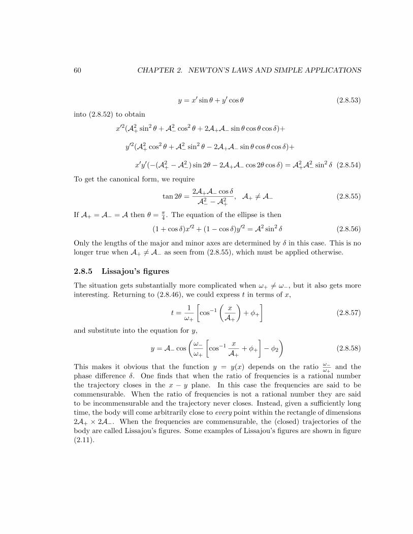
60 CHAPTER 2. NEWTON’S LAWS AND SIMPLE APPLICATIONS
y = x′ sin θ + y′ cos θ (2.8.53)
into (2.8.52) to obtain
x′2(A2+ sin2 θ +A2
− cos2 θ + 2A+A− sin θ cos θ cos δ)+
y′2(A2+ cos2 θ +A2
− sin2 θ − 2A+A− sin θ cos θ cos δ)+
x′y′(−(A2+ −A2
−) sin 2θ − 2A+A− cos 2θ cos δ) = A2+A2− sin2 δ (2.8.54)
To get the canonical form, we require
tan 2θ =2A+A− cos δ
A2− −A2
+
, A+ 6= A− (2.8.55)
If A+ = A− = A then θ = π4 . The equation of the ellipse is then
(1 + cos δ)x′2 + (1− cos δ)y′2 = A2 sin2 δ (2.8.56)
Only the lengths of the major and minor axes are determined by δ in this case. This is nolonger true when A+ 6= A− as seen from (2.8.55), which must be applied otherwise.
2.8.5 Lissajou’s figures
The situation gets substantially more complicated when ω+ 6= ω−, but it also gets moreinteresting. Returning to (2.8.46), we could express t in terms of x,
t =1
ω+
[cos−1
(x
A+
)+ φ+
](2.8.57)
and substitute into the equation for y,
y = A− cos
(ω−ω+
[cos−1 x
A++ φ+
]− φ2
)(2.8.58)
This makes it obvious that the function y = y(x) depends on the ratio ω−ω+
and thephase difference δ. One finds that when the ratio of frequencies is a rational numberthe trajectory closes in the x − y plane. In this case the frequencies are said to becommensurable. When the ratio of frequencies is not a rational number they are saidto be incommensurable and the trajectory never closes. Instead, given a sufficiently longtime, the body will come arbitrarily close to every point within the rectangle of dimensions2A+ × 2A−. When the frequencies are commensurable, the (closed) trajectories of thebody are called Lissajou’s figures. Some examples of Lissajou’s figures are shown in figure(2.11).
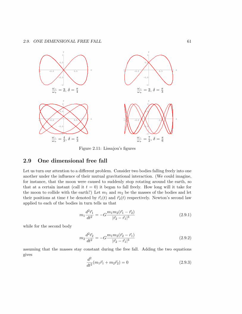
2.9. ONE DIMENSIONAL FREE FALL 61
-1 -0.5 0.5 1x
-1
-0.5
0.5
1
y
ω−ω+
= 2, δ = π4
-1 -0.5 0.5 1x
-1
-0.5
0.5
1
y
ω−ω+
= 2, δ = π3
-1 -0.5 0.5 1x
-1
-0.5
0.5
1
y
ω−ω+
= 43 , δ = π
3
-1 -0.5 0.5 1x
-1
-0.5
0.5
1
y
ω−ω+
= 72 , δ = π
6
Figure 2.11: Lissajou’s figures
2.9 One dimensional free fall
Let us turn our attention to a different problem. Consider two bodies falling freely into oneanother under the influence of their mutual gravitational interaction. (We could imagine,for instance, that the moon were caused to suddenly stop rotating around the earth, sothat at a certain instant (call it t = 0) it began to fall freely. How long will it take forthe moon to collide with the earth?) Let m1 and m2 be the masses of the bodies and lettheir positions at time t be denoted by ~r1(t) and ~r2(t) respectively. Newton’s second lawapplied to each of the bodies in turn tells us that
m1d2~r1
dt2= −Gm1m2(~r1 − ~r2)
|~r2 − ~r1|3(2.9.1)
while for the second body
m2d2~r2
dt2= −Gm1m2(~r2 − ~r1)
|~r2 − ~r1|3(2.9.2)
assuming that the masses stay constant during the free fall. Adding the two equationsgives
d2
dt2(m1~r1 +m2~r2) = 0 (2.9.3)
62 CHAPTER 2. NEWTON’S LAWS AND SIMPLE APPLICATIONS
which tells us that the point whose position is
rcm =m1~r1 +m2~r2
m1 +m2(2.9.4)
moves with a constant velocity, as would a free body. This point is called the center ofmass of the system. Note that the center of mass is just a point in space; it is not itselfa material body.
Multiplying the first equation by m2 and the second by m1, and then subtracting thefirst from the second gives
m1m2d2
dt2(~r2 − ~r1) = −Gm1m2(m1 +m2)(~r2 − ~r1)
|~r2 − ~r1|3(2.9.5)
or, if ~r is used to represent the relative position ~r2 − ~r1 of body 2 w.r.t. body 1, andM = m1 +m2 is the total mass of the system,
d2~r
dt2= −GM
r2r (2.9.6)
The coordinate ~r is called the relative coordinate. As the motion is purely radial, i.e.,along the line joining the two bodies, it is effectively one dimensional with the force law
d2r
dt2= −GM
r2. (2.9.7)
It can solved using the techniques laid out earlier in the chapter. We have
vdv
dr= −GM
r2⇒ 1
2v2 = GM
[1
r− 1
r0
](2.9.8)
where r0 represents the position at which the bodies commenced their free fall (r(0) = r0)and we have assumed that v(0) = 0. This means that
v =dr
dt= −
√2GM
[1
r− 1
r0
]⇒ −
√r0
2GM
∫ r
r0
dr′√
r′
r0 − r′= t (2.9.9)
(we have chosen the negative square root because r is decreasing in time). By making thesubstitution r′ = r0 sin2 η, we evaluate the integral on the left and arrive at√
r0
2GM
[√r(r − r0)− r0 sin−1
√r′
r0
]rr0
= t(r) (2.9.10)
or √r0
2GM
[πr0
2+√r(r − r0)− r0 sin−1
√r
r0
]= t(r) (2.9.11)
2.10. SYSTEMS WITH VARIABLE MASS: THE ROCKET 63
At r = 0 we have a collision, because r is the magnitude of the relative coordinate. Thetime taken for collision is therefore
t(0) =π
2
(r3
0
2GM
) 12
(2.9.12)
We can now answer the question we began with. Suppose the moon were indeed suddenlycaused to stop in its orbit. Assuming that its orbit is quasi-circular, its period is given by
τ =2πr0
v= 2π
(r3
0
GM
) 12
= 2√
2π
(r3
0
2GM
) 12
, (2.9.13)
where we used the fact that the centripetal acceleration of the moon is caused by thegravitational force on it, i.e.,
v2
r0=GM
r20
⇒ v =
√GM
r0. (2.9.14)
We can give the time for collision in terms of its orbital period prior to being stopped,
t(0) =τ
4√
2≈ 4.95 days (2.9.15)
(taking τ = 28 days for the moon’s orbit about the earth). Of course this is only anacademic discussion because if the moon is indeed suddenly stopped in its orbit it can beonly due to a catastrophic event such as a collision with another heavenly body, which willnot leave the moon intact. Moreover, a freely falling moon would cause such disruptionsto the earth’s environment as to make life impossible long before the actual collision takesplace.
2.10 Systems with variable mass: the rocket
Finally, we address a different sort of system, one in which the mass does not stay constantin time. This kind of system emphasizes the fact that Newton’s second law is actually
d~p
dt= ~F ext (2.10.1)
and not the more often quoted ~F = m~a, whose validity relies on the mass of the bodybeing held constant throughout the body’s motion.
Consider the rocket, shown schematically in figure (2.12). Rockets contain a com-bustible material that burns at some rate depending on its design. The gasses produced
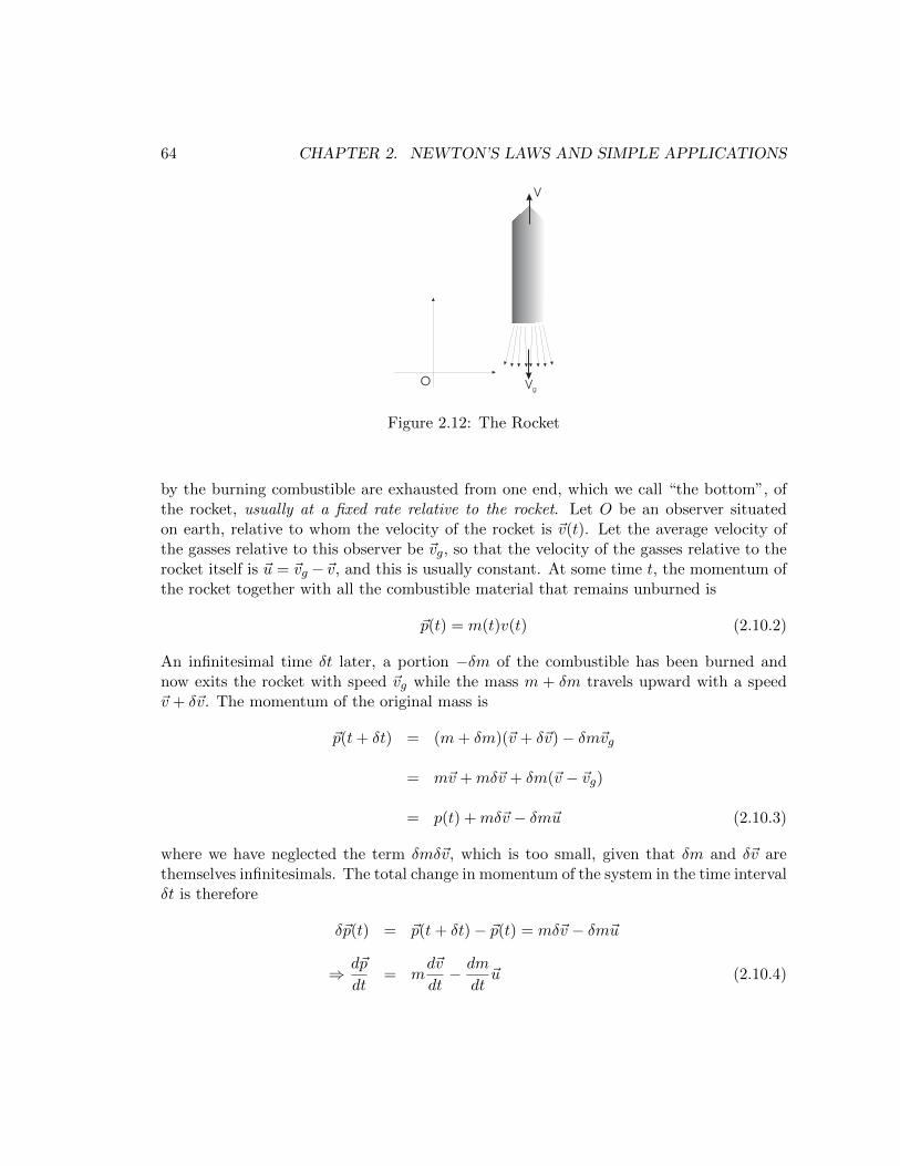
64 CHAPTER 2. NEWTON’S LAWS AND SIMPLE APPLICATIONS
O Vg
V
Figure 2.12: The Rocket
by the burning combustible are exhausted from one end, which we call “the bottom”, ofthe rocket, usually at a fixed rate relative to the rocket. Let O be an observer situatedon earth, relative to whom the velocity of the rocket is ~v(t). Let the average velocity ofthe gasses relative to this observer be ~vg, so that the velocity of the gasses relative to therocket itself is ~u = ~vg −~v, and this is usually constant. At some time t, the momentum ofthe rocket together with all the combustible material that remains unburned is
~p(t) = m(t)v(t) (2.10.2)
An infinitesimal time δt later, a portion −δm of the combustible has been burned andnow exits the rocket with speed ~vg while the mass m + δm travels upward with a speed~v + δ~v. The momentum of the original mass is
~p(t+ δt) = (m+ δm)(~v + δ~v)− δm~vg
= m~v +mδ~v + δm(~v − ~vg)
= p(t) +mδ~v − δm~u (2.10.3)
where we have neglected the term δmδ~v, which is too small, given that δm and δ~v arethemselves infinitesimals. The total change in momentum of the system in the time intervalδt is therefore
δ~p(t) = ~p(t+ δt)− ~p(t) = mδ~v − δm~u
⇒ d~p
dt= m
d~v
dt− dm
dt~u (2.10.4)
2.10. SYSTEMS WITH VARIABLE MASS: THE ROCKET 65
By Newton’s second law this can only be equal to the net external force, therefore
md~v
dt=dm
dt~u+ ~F ext (2.10.5)
This is known as the rocket equation. Even when ~F ext = 0 there is an effective forceon the rocket, which comes about because of the need to conserve momentum and isproportional to the rate at which fuel is being burned and the velocity, relative to therocket itself, at which the resulting gasses are expelled. Notice that because the fuel isbeing consumed the rocket is continuously losing mass, so δm < 0. Therefore the firstterm on the right hand side is directed opposite to the velocity of the gasses relative tothe rocket. Thus hot gasses ejected from the base of the rocket cause the rocket itself torise. If ~F ext is just the (approximately) constant gravitational field of the earth close toits surface, ~F ext = m~g, we can integrate once to get
~v = ~v0 + ~u ln
(m
m0
)+ ~g(t− t0) (2.10.6)
where m0 is the mass of the rocket at time t0. A net zero acceleration (hovering) is possibleonly if
dm
dt~u = −m~g ⇒ m(t) = m0e
− gu
(t−t0) (2.10.7)
i.e., the rate of fuel burning must be adjusted to precisely balance the changing mass ofthe rocket.
Chapter 3
Conservation Theorems
In the previous chapter we stated Newton’s three laws of motion and used Newton’s secondlaw to obtain explicit solutions to a few simple problems involving one or two particlessubject to certain initial conditions, i.e., the position(s) and velocity(ies) of the particle(s).Unfortunately it is not possible to obtain such simple, closed form solutions in most casesof real physical interest. Can we then say anything about a physical system withoutreferring to a tidy, closed form solution? It turns out that the answer is yes, it is possibleto say quite a lot! For this we now examine some very general consequences of Newton’slaws, the so-called conservation theorems. We will do this by building and examininga generic mechanical system made up of particles with generic interactions. In doing so,we will develop a new set of tools that will later allow us to analyze more complicatedproblems than would otherwise be possible.
3.1 Single Particle Conservation Theorems
3.1.1 Conservation of momentum
We begin by considering a system consisting of one particle. According to Newton’s secondlaw,
d~p
dt= ~F ext (3.1.1)
where ~F ext is the external force applied to it. Evidently, if ~F ext = 0, there is no externalforce and
d~p
dt= 0⇒ ~p = const. (3.1.2)
Thus we have our first conservation theorem:
• When the next external force on a particle is zero, the momentum of the particle isconserved.
66
3.1. SINGLE PARTICLE CONSERVATION THEOREMS 67
3.1.2 Conservation of angular momentum
We define the angular momentum of a single particle about a point (call that point theorigin) as
~L = ~r × ~p (3.1.3)
where ~r is the position of the particle with respect to the reference point. Taking aderivative with respect to time,
d~L
dt= ~v × ~p+ ~r × d~p
dt= ~r × ~F (3.1.4)
because ~v × ~p ≡ 0. This is the equivalent of Newton’s second law for rotational motion.The quantity ~r × ~F is called the torque
~τ = ~r × ~F (3.1.5)
andd~L
dt= ~τ (3.1.6)
Our second conservation law follows:
• When the net torque due to all the external forces on a particle vanishes the angularmomentum of the particle is conserved.
3.1.3 Work and the conservation of energy
Again, consider what happens when ~F ext 6= 0. Then taking the inner product of thesecond law with ~v,
d~p
dt= ~F ext ⇒ m~v · d~v
dt= ~v · ~F ext (3.1.7)
and integrating the resulting equation gives,
m
∫ 2
1~v · d~v =
∫ 2
1
~F ext · ~v dt⇒ 1
2(m~v2
2 −m~v21) =
∫ 2
1
~F ext · d~r (3.1.8)
The quantity K = 12m~v
2 is called the kinetic energy of the particle, and
W12 =
∫ 2
1
~F ext · d~r (3.1.9)
is the work done by the external force ~F ext on the particle in moving it from the pointlabeled “1” to the point labeled “2”. The power is the instantaneous rate at which workis done,
P =dW
dt= ~F ext · d~r
dt= ~F ext · ~v (3.1.10)
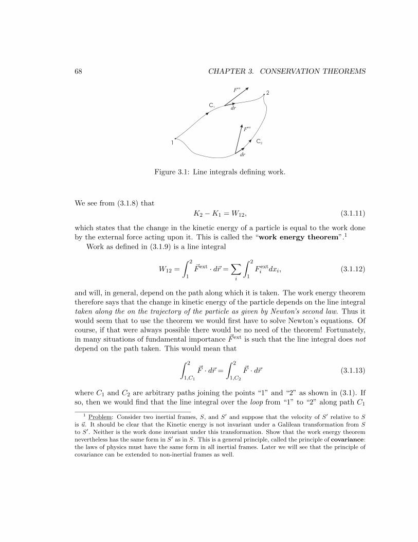
68 CHAPTER 3. CONSERVATION THEOREMS
1
2
C1
C2
Fext
Fext
dr
dr
Figure 3.1: Line integrals defining work.
We see from (3.1.8) that
K2 −K1 = W12, (3.1.11)
which states that the change in the kinetic energy of a particle is equal to the work doneby the external force acting upon it. This is called the “work energy theorem”.1
Work as defined in (3.1.9) is a line integral
W12 =
∫ 2
1
~F ext · d~r =∑i
∫ 2
1F exti dxi, (3.1.12)
and will, in general, depend on the path along which it is taken. The work energy theoremtherefore says that the change in kinetic energy of the particle depends on the line integraltaken along the on the trajectory of the particle as given by Newton’s second law. Thus itwould seem that to use the theorem we would first have to solve Newton’s equations. Ofcourse, if that were always possible there would be no need of the theorem! Fortunately,in many situations of fundamental importance ~F ext is such that the line integral does notdepend on the path taken. This would mean that∫ 2
1,C1
~F · d~r =
∫ 2
1,C2
~F · d~r (3.1.13)
where C1 and C2 are arbitrary paths joining the points “1” and “2” as shown in (3.1). Ifso, then we would find that the line integral over the loop from “1” to “2” along path C1
1 Problem: Consider two inertial frames, S, and S′ and suppose that the velocity of S′ relative to Sis ~u. It should be clear that the Kinetic energy is not invariant under a Galilean transformation from Sto S′. Neither is the work done invariant under this transformation. Show that the work energy theoremnevertheless has the same form in S′ as in S. This is a general principle, called the principle of covariance:the laws of physics must have the same form in all inertial frames. Later we will see that the principle ofcovariance can be extended to non-inertial frames as well.
3.1. SINGLE PARTICLE CONSERVATION THEOREMS 69
and from “2” to “1” along path C2 yields exactly zero because, rewriting (3.1.13) as∫ 2
1,C1
~F · d~r = −∫ 1
2,C2
~F · d~r (3.1.14)
gives ∫ 2
1,C1
~F · d~r +
∫ 1
2,C2
~F · d~r = 0 =
∮C1−C2
~F · d~r (3.1.15)
But C1 and C2 were quite arbitrary as were the initial and final points they connected,therefore ∮
C
~F · d~r = 0 (3.1.16)
along any closed loop, C.
Definition: If the work done by a force ~F ,
W12 =
∫ 2
1,C
~F · d~r, (3.1.17)
is independent of the path taken (the curve C) then it is conservative. A force ~F isconservative if and only if ∮
C
~F · d~r = 0 (3.1.18)
for any closed curve C.
Conservative forces are of particular interest because, as far as we know, all the funda-mental forces of nature are conservative. Moreover, they are easy to work with. If a forceis conservative then applying Stokes theorem to (3.1.18) gives∮
C
~F · d~r =
∫S
(~∇× ~F ) · d~S = 0 (3.1.19)
But as C is arbitrary, so is S and it follows that ~∇ × ~F = 0. Thus ~F is conservative ifand only if it is rotation free. Of course, every rotation free vector can be expressed asthe gradient of a scalar function, therefore we define
~F = −~∇U(~r) (3.1.20)
The work done by the conservative force ~F in moving a particle from one point to anotherbecomes ∫ 2
1,C
~F · d~r = −∫ 2
1
~∇U · d~r = −∫ 2
1dU = U(~r1)− U(~r2) (3.1.21)
70 CHAPTER 3. CONSERVATION THEOREMS
U(~r) is called the potential energy function corresponding to ~F . If ~F (~r) is known then itcan be recovered, up to a constant, from
U(~r) = −∫ ~r
∗~F (~r′) · d~r′ (3.1.22)
where ∗ represents some fixed point, a “reference” point, of our choosing. In other words,U(~r) is defined only up to a constant. The constant is determined by our choice of ∗,which is itself arbitrary but once chosen must be held fixed (although U(~r) is defined viaa line integral, it is well defined i.e., independent of the path from ∗ to ~r) because ~F isconservative). Now, by the work energy theorem
W12 = U(~r1)− U(~r2) = K2 −K1 ⇒ K1 + U(~r1) = K2 + U(~r2) (3.1.23)
which means that
E = K + U =1
2m~v2 + U(~r) (3.1.24)
is constant during the motion of the particle. The constant, E, is called the total energyof the particle. Evidently, the total energy of a particle is defined only up to an additiveconstant.
The concept of potential energy and by implication of the total energy of a particle isstrictly defined only when the total external force acting upon the particle is conservative.If the reference point ∗ is changed to ∗′ we find that
U ′(~r) = −∫ ~r
∗′~F · d~r = −
∫ ∗∗′~F · d~r −
∫ ~r
∗~F · d~r
= U(~r) + C (3.1.25)
where C is the constant given by first integral on the right (because ~F is conservative theintegrals do not depend on the path between the endpoints, so they must depend only onthe endpoints). This leads to our second conservation theorem:
• When the external force(s) on a particle is (are) conservative, then ~F = −~∇U(~r),for some function U(~r) called the potential energy of the particle,
U(~r) = −∫ ~r
∗~F · d~r, (3.1.26)
and the total energy, which is the sum of the kinetic energy and the potential energy,
E =1
2m~v2 + U(~r) (3.1.27)
is conserved throughout its motion.
3.2. FRICTIONAL FORCES AND MECHANICAL ENERGY 71
For a general potential function of the form U = U(~r, t), taking a time derivative of E in(3.1.27) we see that
dE
dt= m~v · d~v
dt+dU
dt
= m~v · d~vdt
+ ~v · ~∇U(~r) +∂U
∂t
= ~v ·(md~v
dt+ ~∇U(~r)
)+∂U
∂t=
(md~v
dt− ~F
)+∂U
∂t≡ ∂U
∂t(3.1.28)
where we have used Newton’s second law. For conservative forces, U(~r, t) cannot dependexplicitly on time.
3.2 Frictional forces and mechanical energy
Frictional forces generally arise by the interactions of our physical system with the restof the universe. They are generally complex interactions and can be modelled only phe-nomenologically. No frictional force, ~f , can be conservative because friction always actsin a direction opposite to the velocity and therefore the work done by friction,
W f12 =
∫ 2
1d~r · ~f = −
∫ 2
1ds(v · v)|~f | = −
∫ 2
1ds|~f | (3.2.1)
where s is the path length and we have used d~r/ds = v, is always negative and can neverbe independent of the path because the integrand is always positive. For instance, if |~f | =const., then the work done is just W12 = |~f |L12 where L12 is the path length betweenpoints 1 and 2. On the other hand, if |~f | = k|~v|α then
W f12 = −k
∫ 2
1ds|~v|α (3.2.2)
and the rate at which this work is being done is
dW f12
dt= −k|~v|α+1 (3.2.3)
Suppose that all the other forces on our particle are conservative, so that we may definea potential energy for the sum of the conservative forces,
U cons(~r) = −∫ ~r
∗~F cons · d~r. (3.2.4)
72 CHAPTER 3. CONSERVATION THEOREMS
Integrate the equations of motion once,
m~v · d~vdt
= ~f · ~v + ~F cons · ~v
⇒ 1
2m(~v2
2 − ~v21) =
∫ 2
1d~r · ~f + U cons(~r1)− U cons(~r2)
⇒ 1
2m~v2
2 + U cons(~r2) =1
2m~v2
1 + U cons(~r1)− k∫ 2
1ds|~v|α (3.2.5)
The quantity E = K+U cons, which we will refer to as the mechanical energy of the particleis no longer conserved. In fact, it is easy to see that
dEdt
= −k|~v|α+1 (3.2.6)
Now it is a fundamental postulate of physics that the total energy of the universe remainsconstant. This loss of mechanical energy of our particle would then imply that the particle’senergy is being transferred to the environment (the rest of the universe) at a rate that isproportional to some power of the particle’s speed.
3.3 Examples of conservative forces
Only two of the forces considered in the pervious chapter are conservative, viz., the restora-tive force of an ideal spring and the gravitational force acting between two massive bodies.Let us take a brief look at them.
The simple harmonic oscillator: The restorative force exerted by a spring, ~F = −k~r, is
conservative. To see this simply take the curl of ~F to get
~∇× ~F = −k~∇× ~r ≡ 0. (3.3.1)
So we can obtain the potential energy of the simple harmonic oscillator by the integral
U(~r) = −∫ ~r
∗~F · d~r =
1
2k~r2 (3.3.2)
where we have taken the reference point to be the origin. The total energy of the harmonicoscillator,
E =1
2m~v2 +
1
2k~r2, (3.3.3)
3.4. THE DAMPED AND DRIVEN OSCILLATOR 73
is conserved and in one dimension the relation may be thought of as the first of the twointegrals that are required to solve Newton’s equations. Solving for v gives
v =dx
dt=
√2E
m− ω2x2 (3.3.4)
and we note that if v0 represents the velocity of the body at x = 0 then v20 = 2E/m. Thus
we recover (2.8.4).
Gravitational free fall: The gravitational force between two particles is conservative. Atthis point suppose, for simplicity, that particle 1 is somehow fixed at the origin and particle2 is situated at ~r. Then the gravitational force on particle 2 due to 1 is
~F = −Gm1m2
r3r (3.3.5)
which is easily proved to be conservative (~∇× ~F = 0). The potential energy of particle 2due to its gravitational interaction with particle 1 is therefore
U(~r) = −∫ ~r
∗~F · d~r = Gm1m2
∫ ~r
∗
d~r
r2· r = Gm1m2
∫ r
∗
dr
r2(3.3.6)
The most convenient reference point would be out at infinity, i.e., particle 2 is infinitelyseparated from particle 1, in which case
U(~r) = −Gm1m2
r(3.3.7)
The total energy of the particle 2 would be the sum
E =1
2m~v2
2 −Gm1m2
r(3.3.8)
In general we cannot assume that 1 is fixed to the origin (this may be a good approximationwhen the mass of 1 is very much greater than the mass of 2 – as in, for example, the earthsun system – but even so it is only an approximation.) A more detailed examination ofthis system of two particles will be given at the end of this chapter.
3.4 The damped and driven oscillator
We have examined the damped and undamped oscillator in the previous chapter. Let usnow complicate the problem by adding a time dependent force driving the oscillator. Theequation of motion is
md2x
dt2= −kx− bdx
dt+ F (t) (3.4.1)
74 CHAPTER 3. CONSERVATION THEOREMS
which can be written as
(D2 + 2γD + ω20)x(t) =
F (t)
m(3.4.2)
where γ = b/2m and ω20 = k/m. Again we have a linear differential equation with constant
coefficients, but it is not homogeneous because of the driving force on the right.
3.4.1 Fourier Expansion
The function F (t) could be anything, but situations of greatest physical interest occurwhen F (t) is periodic. It also turns out that, in this case, we can give a complete andgeneral solution to the problem by exploiting a beautiful theorem in mathematics due toJean-Baptiste Fourier, which says that:
The Fourier Theorem: Any piecewise continuous, periodic function with period τ , whichis square integrable, i.e., ∫ t2
t1
dt|F (t)|2 <∞ (3.4.3)
where t2 − t1 = T , can be decomposed into the infinite series
F (t) =1
2a0 +
∞∑n=1
(an cosnωt+ bn sinnωt) , ω =2π
τ(3.4.4)
where an and bn are the “Fourier coefficients” that can be obtained from F (t) accordingto
an =2
τ
∫ τ
0dt F (t) cosnωt
bn =2
τ
∫ τ
0dt F (t) sinnωt (3.4.5)
for all n (including n = 0). The nth order term in the expansion is called the nth harmonicof F (t).
We will not prove Fourier’s theorem here,2 but simply examine the idea. It has todo with the fact that the set of functions sinnx, cosnx (for integer values of n) is“orthonormal” with respect to an inner product, defined by an integral over one period.In fact, it is easy to show that
1
π
∫ 2π
0dx sinnx sinmx = δmn =
1
π
∫ 2π
0dx cosnx cosmx
2A proof can be found in the book Fourier Series and Boundary Value Problems by J.W. Brown andR.V. Churchill, McGraw-Hill Science 7th edition, (2006).
3.4. THE DAMPED AND DRIVEN OSCILLATOR 75
1
π
∫ 2π
0dx sinnx cosmx = 0 (3.4.6)
for all values of n and m. This property of the sines and cosines is similar to the orthonor-mality of basis vectors x1, x2, ... in ordinary space, except that the set is now countablyinfinite and the definition of what we mean by the inner product is different. If we let thevariable x = ωt = 2πt/τ , then
ω
π
∫ 2πω
0dt sinnωt sinmωt = δmn =
ω
π
∫ 2πω
0dt cosnωt cosmωt
ω
π
∫ 2πω
0dt sinnωt cosmωt = 0 (3.4.7)
Often the inner product between the functions is denoted by 〈 , 〉, for example if f(t) andg(t) are two piecewise continuous, periodic functions of t with period τ the inner productof f with g is
〈f(t), g(t)〉 =2
τ
∫ τ
0dt f(t)g(t), (3.4.8)
where we have set 2π/ω = τ . Carrying the analogy with an ordinary (finite dimensional)vector space even further and using the inner product, we could define the norm of thefunction f(t) by
‖f‖ = 〈f, f〉12 (3.4.9)
Two functions are orthogonal if 〈f, g〉 = 0 and a function is normalized if its normis unity. The distance between two functions is defined to be d(f, g) = ‖f − g‖ andrepresents the root mean square distance between their graphs. Suppose that a functionF (t) is expressed as
F (t) =1
2a0 +
∞∑n=1
[an cosnωt+ bn sinnωt] (3.4.10)
Taking the inner product of F (t) with sinmωt and then cosmωt with m 6= 0 would give
〈F (t), sinmωt〉 =∞∑n=1
bn〈sinnωt, sinmωt〉 =∞∑n=1
bnδnm = bm
〈F (t), cosmωt〉 =∞∑n=1
an〈cosnωt, cosmωt〉 =∞∑n=1
anδnm = am (3.4.11)
while if m = 0,
〈F (t), 1〉 =2
τ
∫ τ
0dt F (t) =
1
2a0 ·
2
τ
∫ τ
0dt = a0 (3.4.12)
76 CHAPTER 3. CONSERVATION THEOREMS
(we see why the first coefficient, a0, was defined with the extra factor of 1/2). Thusall the coefficients can be formally defined simply because the set sinnωt, cosnωt isorthonormal with respect to this inner product. However this does not guarantee that theseries faithfully reproduces the function F (t). Formally, this would happen if the sequenceSN defined by
SN (t) =1
2a0 +
N∑n=1
[an cosnωt+ bn sinnωt] (3.4.13)
were to converge in the mean to the function F (t), i.e., if the root mean square distancebetween the two were to approach zero as N approached infinity, or
limN→∞
‖F (t)− SN (t)‖2 = limN→∞
∫ τ
0[F (t)− SN (t)]2 = 0 (3.4.14)
If this condition holds for a class of periodic functions F (t) then the set sinnωt, cosnωtwould be not simply orthonormal but also complete within that class. It turns out thatthis condition is met if F (t) is piecewise continuous and square integrable, so every squareintegrable, piecewise continuous and periodic function has a faithful Fourier decomposi-tion.
By a simple transformation,
αn =√a2n + b2n, φn = tan−1
(bnan
), (3.4.15)
which is valid so long as n 6= 0 and provided that an 6= 0, the Fourier series can be put inthe form
F (t) =∞∑n=0
αn cos(nωt− φn) (3.4.16)
with φ0 = 0 and α0 = a0/2. But (3.4.2) is a linear equation, which means that we canconsider its solution, x(t), to be a superposition, x(t) =
∑n xn(t), where each xn(t) is a
solution of
(D2 + γD + ω20)x0(t) = f0
(D2 + γD + ω20)xn(t) = fn cos(nωt− φn), (3.4.17)
where f0,n = α0,n/m. There is a standard way to solve such differential equations. Recallthat a general solution of an nth order differential equation must have n (integration)constants. Newton’s equations are second order, so they require two constants per spacedimension, which are related of course to the components of the initial position and velocityof the particle. We already know how to solve the homogeneous equation
(D2 + 2γD + ω20)xn(t) = 0, (3.4.18)
3.4. THE DAMPED AND DRIVEN OSCILLATOR 77
so here is the trick: first calculate the general solution to (3.4.18). This is the compli-mentary function, xc(t), and will contain the desired integration constants. It does notdepend on n. Then look for a particular solution to the inhomogeneous equation, xn,p(t)(this will depend on n). Any solution will do and the sum of xc(t) and xn,p(t)
xn(t) = xc(t) + xn,p(t) (3.4.19)
is also a solution of the inhomogeneous equation. Moreover, because it contains twoarbitrary constants, it is also the most general solution.
Since we already have the general solutions of the homogeneous equation (see (2.8.22),we will now look for a particular solution. Try
xn,p(t) = Bn cos(nωt− δn), (3.4.20)
where Bn and δn are to be determined. Inserting this into (3.4.17) gives
(ω20 − n2ω2)Bn cos(nωt− δn)− 2γnωBn sin(nωt− δn) = fn cos(nωt− φn). (3.4.21)
If we expand the trigonometric functions on the left and right of the above equation, wehave
Bn[(ω20 − n2ω2) cos δn − 2nωγ sin δn] cosnωt
+Bn[(ω20 − n2ω2) sin δn − 2nωγ cos δn] sinnωt
= fn cosφn cosnωt+ fn sinφn sinnωt (3.4.22)
Comparing terms we get
Bn[(ω20 − n2ω2) cos δn − 2nωγ sin δn] = fn cosφn
Bn[(ω20 − n2ω2) sin δn − 2nωγ cos δn] = fn sinφn (3.4.23)
which together give φn in terms of δn,
tanφn =(ω2
0 − n2ω2) tan δn − 2nωγ
(ω20 − n2ω2)− 2nωγ tan δn
, (3.4.24)
equivalently δn in terms of φn
tan δn =2nωγ + (ω2
0 − n2ω2) tanφn(ω2
0 − n2ω2)− 2nωγ tanφn(3.4.25)
78 CHAPTER 3. CONSERVATION THEOREMS
which is the relation we were after. We now seek the next relation we need, i.e., anexpression for Bn. Using (3.4.25) we find
sin δn =(ω2
0 − n2ω2) tanφn + 2nωγ√(ω2
0 − n2ω2)2 + 4n2ω2γ2cosφn (3.4.26)
and
cos δn =(ω2
0 − n2ω2) tanφn − 2nωγ√(ω2
0 − n2ω2)2 + 4n2ω2γ2sinφn (3.4.27)
which expressions may be inserted in either of the pair of equations in (3.4.23) to get
Bn =fn√
(ω20 − n2ω2)2 + 4n2ω2γ2
(3.4.28)
The general solution of the damped and forced oscillator is therefore
x(t) = e−γt[A+e√γ2−ω2
0t +A−e−√γ2−ω2
0t]
+
∞∑n=0
Bn cos(nωt+ δn) (3.4.29)
with Bn and δn given above for each n.
Notice that, after a very long time, t → ∞, the first term will die away because ofthe exponential damping term multiplying it. The effect of the first term is thereforenegligible after a sufficiently long time (roughly τ ∼ γ−1), and xc(t) is said to represent“transient effects”. For large times, the most important part of the solution is thereforethe particular solution,
x(t)→ xp(t) =
∞∑n=0
Bn cos(nωt− δn). (3.4.30)
Let us study some late time properties of the solution for the case when there are dampedoscillations with ω0 >
√2γ. The amplitude of the driven oscillations is extreme for those
harmonics which satisfy
dBnd(nω)
= 0⇒ 2γ2 − (ω20 − n2ω2) = 0, n 6= 0 (3.4.31)
i.e., when
nR ω = ωR =√ω2
0 − 2γ2 (3.4.32)
It is easy to show that the second derivative of Bn is negative in this case and thereforeωR yields a maximum amplitude. The total energy of the oscillator is proportional to the
3.4. THE DAMPED AND DRIVEN OSCILLATOR 79
square of the amplitude and therefore ωR also represents the harmonic for which the totalenergy of the oscillator is maximum. On the other hand, the kinetic energy is
T =1
2mx2 =
1
2m
[ ∞∑n=0
nωBn sin(nωt− δn)
]2
(3.4.33)
It follows that the time averaged kinetic energy is3
T =1
4m
∞∑n=0
n2ω2B2n, (3.4.34)
(where we have used
sin(nωt− δn) sin(mωt− δm) =1
2δmn, (3.4.35)
which follows from orthonormality) is not maximum for the harmonic ωR but for
ωK = nKω = ω0. (3.4.36)
The total energy of the oscillator and the kinetic energy resonate at different harmonics,an effect of the damping. Physically, this happens because energy is continuously beingtransferred from the driving mechanism to the damping medium, where it is lost as heat.To see this consider the power delivered by the driving force,
Fx = −∑n,m
mωαnBmcos(nωt− φn) sin(mωt− δn)
=1
2
∑n
nωαnBn sin(φn − δn). (3.4.37)
It is not difficult to see that the time average of the power transferred to the system bythe driving force is maximum for the harmonic ωK above, i.e., when the kinetic energy ismaximum. This is compatible with the fact that the rate at which mechanical energy islost to the dissipating medium depends on some power of the speed, as shown in 3.2.6.
3.4.2 Green’s Function
There is another generic technique for solving linear inhomogeneous differential equationssuch as the one we have been dealing with, and that is to seek a particular solution of the
3For a periodic function, f , of period τ , we define the time average as
f =1
τ
∫ τ
0
dtf(t)
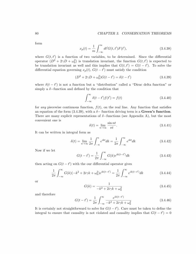
80 CHAPTER 3. CONSERVATION THEOREMS
form
xp(t) =1
m
∫ ∞−∞
dt′G(t, t′)F (t′), (3.4.38)
where G(t, t′) is a function of two variables, to be determined. Since the differentialoperator (D2 + 2γD + ω2
0) is translation invariant, the function G(t, t′) is expected tobe translation invariant as well and this implies that G(t, t′) = G(t − t′). To solve thedifferential equation governing xp(t), G(t− t′) must satisfy the condition
(D2 + 2γD + ω20)G(t− t′) = δ(t− t′) (3.4.39)
where δ(t − t′) is not a function but a “distribution” called a “Dirac delta function” orsimply a δ−function and defined by the condition that∫ ∞
−∞δ(t− t′)f(t′) = f(t) (3.4.40)
for any piecewise continuous function, f(t), on the real line. Any function that satisfiesan equation of the form (3.4.39), with a δ− function driving term is a Green’s function.There are many explicit representations of δ−functions (see Appendix A), but the mostconvenient one is
δ(t) = limn→∞
sinnt
πt. (3.4.41)
It can be written in integral form as
δ(t) = limn→∞
1
2π
∫ n
−neiktdk =
1
2π
∫ ∞−∞
eiktdk (3.4.42)
Now if we let
G(t− t′) =1
2π
∫ ∞−∞
G(k)eik(t−t′)dk (3.4.43)
then acting on G(t− t′) with the our differential operator gives
1
2π
∫ ∞−∞
G(k)(−k2 + 2iγk + ω20)eik(t−t′) =
1
2π
∫ ∞−∞
eik(t−t′)dk (3.4.44)
or
G(k) =1
−k2 + 2iγk + ω20
(3.4.45)
and therefore
G(t− t′) =1
2π
∫ ∞−∞
eik(t−t′)
−k2 + 2iγk + ω20
(3.4.46)
It is certainly not straightforward to solve for G(t− t′). Care must be taken to define theintegral to ensure that causality is not violated and causality implies that G(t − t′) = 0
3.4. THE DAMPED AND DRIVEN OSCILLATOR 81
xx
C
C'
Figure 3.2: Contour in the complex k− plane defining the integral for G(t− t′).
when t < t′ because the oscillator should not respond to the force before the latter actson it.
Notice that the integrand has two poles, viz.,
k2 − 2iγk − ω20 = 0⇒ k = iγ ±
√−γ2 + ω2
0, (3.4.47)
both of which lie in the upper half plane complex plane. We will define the integral by acontour in the complex k−plane in such a way as to ensure that G(t− t′) = 0 when t < t′.
• First consider the underdamped case, for which the square root is positive, and letω =
√ω2
0 − γ2. We define the integral by its value along one of the contours shownin 3.2. Both contours run along the real axis from −∞ to +∞. One of them isclosed in the upper half plane and the other in the lower half plane by a semi-circleat infinity. They must be chosen so that the integrals over the semi-circles vanishand do not contribute to the value of the integral:
– if t > t′, we close the contour in the upper half plane and
– if t < t′, we close it in the lower half plane.
Because there are no poles in the lower half plane G(t − t′) = 0 when t < t′ byCauchy’s residue theorem. Moreover, using the residue theorem when t > t′, we get
G(t− t′) =1
ωe−γ(t−t′) sinω(t− t′) (3.4.48)
when t > t′. We can combine the two cases by introducing the Heaviside function,
Θ(t) =
0 if t ≤ 01 if t > 0
(3.4.49)
writing
G(t− t′) =1
ωe−γ(t−t′) sinω(t− t′)Θ(t− t′). (3.4.50)
82 CHAPTER 3. CONSERVATION THEOREMS
• For the critically damped case there is a double pole, situated at k = iγ/2. Wefind straightforwardly that
G(t− t′) = e−γ(t−t′)(t− t′)Θ(t− t′). (3.4.51)
• Finally, for the overdamped case there are two imaginary roots at
k = i
(γ ±
√γ2 − ω2
0
)= k± (3.4.52)
and closing the contour as before gives
G(t− t′) = −i
[eik+(t−t′)
k+ − k−− eik−(t−t′)
k+ − k−
]Θ(t− t′) (3.4.53)
or
G(t− t′) =e−γ(t−t′)√γ2 − ω2
0
sinh√γ2 − ω2
0 Θ(t− t′). (3.4.54)
Now that G(t − t′) is known in each case, xp(t) is determined directly by integratingaccording to (3.4.38). The Green’s function is an extremely powerful tool to solve linear,inhomogeneous differential equations with constant coefficients and is straightforwardlyextended to partial differential equations in higher dimension.
3.5 Systems of many particles
Extending the arguments given in the previous sections, let us now consider many particles,labeled by integers n ∈ N (not to be confused with the integers that label the harmonicsin the Fourier series), located at ~rn and having masses mn as shown in figure (3.3). Definethe total momentum of the system as
~p =∑n
~pn =∑n
mn~vn ⇒d~p
dt=∑n
mnd~vndt
=∑n
~Fn (3.5.1)
where ~Fn represents the total external force on the nth particle. This force may be thoughtof as arising from two sources: (i) the forces, ~F ext
n , on the particle due to the rest of theuniverse, i.e., the part of the universe that excludes the system of particles itself and (ii)the force on the particle due to the other particles within the system. The latter force canbe written as the sum of all the forces exerted on the particle by all the other particles ofthe system,
~F intn =
∑m 6=n
~Fm→n (3.5.2)
3.5. SYSTEMS OF MANY PARTICLES 83
rn
Figure 3.3: Many particle systems.
The first we shall call the “external” force, because it’s source is external to the system.The second we call call an “internal” force because it arises from the system itself. Hencethe superscripts. The total force on the nth particle is then
~Fn = ~F extn +
∑m 6=n
~Fm→n (3.5.3)
where we have used ~Fm→n to signify the force exerted by the mth particle on the nth.Since a particle is presumed not to exert a force on itself, we exclude m = n from the sum.It follows that
d~p
dt=∑n
~F extn +
∑n,m 6=n
~Fm→n (3.5.4)
and clearly the first term on the right gives the total external force on the system, i.e.,
~F ext =∑n
~F extn (3.5.5)
while the second term summarizes the effect of the internal forces on the total momentumof the system of particles. Let us evaluate the sum∑
n,m 6=n
~Fm→n
making two very reasonable assumptions about the forces between the particles of thesystem, viz.,
• they act along the lines joining the particles, and
• they do not depend on the velocities of the particles.
84 CHAPTER 3. CONSERVATION THEOREMS
Under these conditions, we may appeal to Newton’s third law which states that
~Fm→n = −~Fn→m, (3.5.6)
to argue that the desired sum is identically zero! The proof may be made by mathematicalinduction. Considering just two particles we have∑
n,m 6=n
~Fm→n = ~F1→2 + ~F2→1 ≡ 0 (3.5.7)
With three particles there are six terms,∑n,m 6=n
~Fm→n = ~F1→2 + ~F1→3 + ~F2→1 + ~F2→3 + ~F3→1 + ~F3→2
= (~F1→2 + ~F2→1) + (~F1→3 + ~F3→1) + (~F2→3 + ~F3→2) (3.5.8)
which when suitably paired are again shown to cancel each other. We will now argue thatif the sum vanishes for N particles then it must vanish for N + 1 particles. Notice that,for N particles, there are N(N − 1) terms in the sum. Suppose then that
N∑n,m 6=n=1
~Fm→n = 0 (3.5.9)
If one more particle were added to we must account for an additional (N+1)N−N(N−1) =2N terms, which may be written as
N+1∑n,m 6=n=1
~Fm→n =N∑
n,m 6=n=1
~Fm→n + (~F1→N+1 + ~FN+1→1)
+(~F2→N+1 + ~FN+1→2) + ...(~FN→N+1 + ~FN+1→N )(3.5.10)
But all the additional terms vanish by Newton’s third law and we once again have avanishing sum. In fact, it is not difficult to see that∑
n,m 6=n
~Fm→n =∑m<n
(~Fm→n + ~Fn→m) ≡ 0 (3.5.11)
and we conclude thatd~p
dt= ~F ext (3.5.12)
i.e., the rate of change of total momentum depends only on the external applied force (andis independent of the internal forces of the system).

3.5. SYSTEMS OF MANY PARTICLES 85
3.5.1 Conservation of momentum.
Let us define the center of mass of the system by
~p = M~vcm = Md~rcm
dt(3.5.13)
where M =∑
nmn is the total mass of the system. Applying the definition of the totalmomentum, we see that
~p =∑n
mn~vn = M~vcm ⇒ ~vcm =
∑nmn~vn∑nmn
, (3.5.14)
or
~rcm =
∑nmn~rn∑nmn
(3.5.15)
gives the location of the center of mass of the system. It is the weighted mean position ofthe particles of the system, where the masses of the individual particles weight the mean,and moves with the velocity,
~vcm =d~rcm
dt=
∑nmn~vn∑nmn
. (3.5.16)
The center of mass is not necessarily the location of a massive particle but only behavesas a particle of mass equal to the total mass of the system and located at ~rcm. We see thisfrom (3.5.12), which says that
d~p
dt= M
d2~rcm
dt2= ~F ext (3.5.17)
and leads to our first conservation law for a system of particles:
• If the net external force on a system of particles is zero then the total momentum ofthe system is conserved.
The center of mass of the system then behaves as a free particle moving, according toNewton’s first law, with constant velocity. We used this fact to solve the problem of twobodies falling freely under the influence of their mutual gravitational acceleration in theprevious chapter and it is regularly used in the analysis of collisions, when the collidingsystem is isolated.
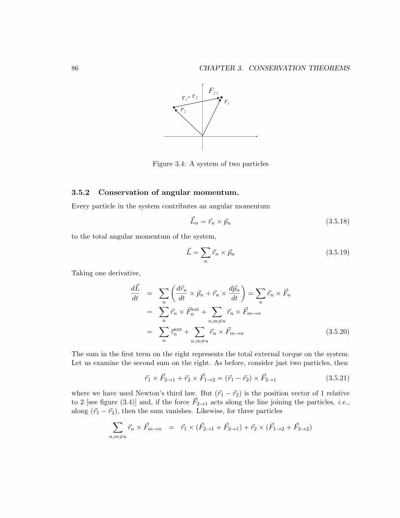
86 CHAPTER 3. CONSERVATION THEOREMS
r1
r2
r - r1
2
F2 1
Figure 3.4: A system of two particles
3.5.2 Conservation of angular momentum.
Every particle in the system contributes an angular momentum
~Ln = ~rn × ~pn (3.5.18)
to the total angular momentum of the system,
~L =∑n
~rn × ~pn (3.5.19)
Taking one derivative,
d~L
dt=
∑n
(d~rndt× ~pn + ~rn ×
d~pndt
)=∑n
~rn × ~Fn
=∑n
~rn × ~F extn +
∑n,m 6=n
~rn × ~Fm→n
=∑n
~τ extn +
∑n,m 6=n
~rn × ~Fm→n (3.5.20)
The sum in the first term on the right represents the total external torque on the system.Let us examine the second sum on the right. As before, consider just two particles, then
~r1 × ~F2→1 + ~r2 × ~F1→2 = (~r1 − ~r2)× ~F2→1 (3.5.21)
where we have used Newton’s third law. But (~r1 − ~r2) is the position vector of 1 relativeto 2 [see figure (3.4)] and, if the force ~F2→1 acts along the line joining the particles, i.e.,along (~r1 − ~r2), then the sum vanishes. Likewise, for three particles∑
n,m 6=n~rn × ~Fm→n = ~r1 × (~F2→1 + ~F3→1) + ~r2 × (~F1→2 + ~F3→2)
3.5. SYSTEMS OF MANY PARTICLES 87
+~r3 × (~F1→3 + ~F2→3) (3.5.22)
and rearranging the terms we find∑n,m 6=n
~rn × ~Fm→n = (~r1 − ~r2)× ~F2→1 + (~r1 − ~r3)× ~F3→1
+(~r2 − ~r3)× ~F3→2 ≡ 0 (3.5.23)
for the same reason we mentioned before, if all the forces between the particles act alongthe lines joining them. In fact4∑
n,m 6=n~rn × ~Fm→n =
∑n<m
(~rn − ~rm)× ~Fm→n ≡ 0 (3.5.24)
It follows thatd~L
dt=∑n
~τ extn = ~τ ext (3.5.25)
and
• If the net external torque on the system vanishes, the total angular momentum ofthe system is conserved.
There is an interesting expression for the total angular momentum of a system of particlesin terms of the angular momentum of its center of mass. Let ~rn be the position of the nth
particle relative to the laboratory and let ~r′n be its position relative to the center of mass,i.e., ~r′n = ~rn − ~rcm. The total angular momentum of the system can be written as
~L =∑n
~rn × ~pn =∑n
mn(~r′n + ~rcm)× (~v′n + ~vcm)
=∑n
mn(~r′n × ~v′n + ~r′n × ~vcm + ~rcm × ~v′n + ~rcm × ~vcm)
=∑n
mn(~r′n × ~v′n) +
(∑n
mn~r′n
)× ~vcm + ~rcm ×
(∑n
mn~v′n
)+ ~rcm × (M~vcm)
=∑n
(~r′n × ~p′n) + ~rcm × ~p (3.5.26)
where ~p′n = mn~v′n is the momentum of the nth particle relative to the center of mass and
we have used ∑n
mn~r′n = 0 =
∑n
mn~v′n (3.5.27)
4Problem: Prove this by mathematical induction
88 CHAPTER 3. CONSERVATION THEOREMS
which follow directly from the definition of the center of mass. So the total angularmomentum is the sum of the angular momentum of the center of mass about the origin,plus the angular momentum of the system about the center of mass.
3.5.3 The Work-Energy theorem
While the rate of change of the total momentum of a system of particles depends only onthe external force, the rate of change of the momentum of each particle within the systemis subject both to the external force acting on it as well as on the internal forces exertedby the other particle of the system upon it, thus
mnd~vndt
= ~Fn = ~F extn +
∑m 6=n
~Fm→n (3.5.28)
Taking the scalar product of each side with ~vn, we get a single scalar equation,
mn~vn ·d~vndt
= ~vn · ~Fn (3.5.29)
which may be integrated once, as we did before for a single particle, to obtain the workenergy theorem,
1
2mn(~v2
n,f − ~v2n,i) =
∫ f
i
~Fn · d~rn (3.5.30)
orKn,f −Kn,i = Wn,if (3.5.31)
Defining the total kinetic energy of the system and the total work done respectively by
K =∑n
Kn =1
2
∑n
mn~v2n (3.5.32)
and
Wif =∑n
Wn,if =∑n
∫ f
i
~Fn · d~rn (3.5.33)
we find thatKf −Ki = Wif (3.5.34)
This, of course, is the work energy theorem for a system of particles. Notice that thetotal kinetic energy of the system is just the sum of the individual kinetic energies of theparticles and that the total work done on the system is the work done by both the internaland the external forces acting on the system.
Just as we had separated the total angular momentum into two parts, the first corre-sponding to the angular momentum of the center of mass about the origin and the second
3.5. SYSTEMS OF MANY PARTICLES 89
corresponding to the angular momentum of the system about the center of mass, so itis also possible to separate the kinetic energy into two pieces, one corresponding to thekinetic energy of the center of mass and the other to the system relative to the center ofmass. To see this, write the position vector of each particle as
~rn = ~rcm + ~r′n, ~vn = ~vcm + ~v′n (3.5.35)
and inserting this into the expression for the total kinetic energy,
K =∑n
mn~v2n =
1
2
∑n
mn(~vcm + ~v′n)2
=1
2M~v2
cm +∑n
mn~vcm · ~v′n +1
2
∑n
mn~v′2n (3.5.36)
But once again we appeal to the fact that the center of mass is the weighted mean positionof the particles constituting the system so that
∑nmn~r
′ = 0 =∑
nmn~v′. We get
K =1
2M~v2
cm +1
2
∑n
mn~v′2n . (3.5.37)
The first term on the right is obviously the kinetic energy of the center of mass. Thesecond is just the kinetic energy of the system as measured by an observer moving withthe center of mass.
The total work may also be broken up into two pieces,
Wif =∑n
∫ f
i
~F extn · d~rn +
∑n,m 6=n
∫ f
i
~Fm→n · d~rn (3.5.38)
If all the external forces acting on the particles of the system are conservative then eachintegral in the sum of the first term on the right is expressed as∫ f
i
~F extn · d~rn = −
∫ f
i
~∇U extn (~rn) · d~rn = −
[U extn,f − U ext
n,i
](3.5.39)
The potential energy of the system, due to the external forces, is
U ext =∑n
U extn (3.5.40)
For the internal forces, consider ∑m6=n
∫ f
i
~Fm→n · d~rn. (3.5.41)
90 CHAPTER 3. CONSERVATION THEOREMS
If the internal forces are also conservative then for every pair (m,n), the force exerted bym on n is the gradient of some function, which we call U int
nm, taken at n,
~Fm→n = −~∇nU intnm. (3.5.42)
Therefore, the second term in (3.5.38) is
∑n,m 6=n
∫ f
i
~Fm→n · d~rn = −∑n,m 6=n
∫ f
i
~∇nU intnm · d~rn (3.5.43)
It generally happens that U intnm depends only on the separation of the particles n and m,
i.e.,
U intnm(~rn, ~rm) = U int
nm(|~rn − ~rm|). (3.5.44)
This is compatible with the third law, since the ~Fm→n = ~∇nUnm = −~∇mUmn = −~Fn→m,and it makes the internal forces invariant with respect to Galilean boosts. It also meansthat
dU intmn = ~∇nU int
mn · d~rn + ~∇mU intmn · d~rm
= ~∇nU intmn · d(~rn − ~rm)
= ~∇nU intmn · d~rnm (3.5.45)
where ~rnm is the position of n relative to m. Returning to the second term in (3.5.38),first consider just two particles
−∑n,m 6=n
∫ f
i
~∇nU intnm · d~rn = −
∫ f
i
[~∇1U
int12 · d~r1 + ~∇2U
int21 · d~r2
]= −
∫ f
i
~∇1Uint12 · d~r12
= −∫ f
idU int
12 = U int12 (~ri)− U int
12 (~rf ) (3.5.46)
For three particles, we have
−∑n,m 6=n
∫ f
i
~∇nU intnm · d~rn = −
∫ f
i
[~∇1(U int
12 + U int13 ) · d~r1 + ~∇2(U int
21 + U int23 ) · d~r2
+~∇3(U int31 + U int
32 ) · d~r3
]
3.5. SYSTEMS OF MANY PARTICLES 91
= −∫ f
i
[~∇1U
int12 · d~r12 + ~∇1U
int13 · d~r13 + ~∇2U
int23 · d~r23
]= −
∫ f
i
[dU int
12 + dU int13 + dU int
23
](3.5.47)
using (3.5.45), and we arrive at (for three particles)
−∑n,m 6=n
∫ f
i
~∇nU intnm · d~rn = −
[U int
12 + U int13 + U int
23
]fi
(3.5.48)
We can already recognize a pattern: for N particles,
−∑n,m 6=n
∫ f
i
~∇nU intnm · d~rn = −
[∑m<n
U intmn
]fi
= −1
2
∑m6=n
U intmn
fi
(3.5.49)
can be proved by induction provided, of course, that all the internal forces are conservativewith potentials that depend only on the separation of the particles.
We see that the system of particles also has a potential energy due to the internalforces, which is given by
U int =∑m<n
U intmn =
1
2
∑m 6=n
U intmn (3.5.50)
The total potential energy of the system, due to both the internal and the external forcesis therefore
U = U ext + U int =∑n
U extn +
∑m<n
U intmn (3.5.51)
The work energy theorem then tells us that
Kf −Ki = Wif = Ui − Uf ⇒ Ki + Ui = Kf + Uf (3.5.52)
which, as before, means that there is a quantity, which we call the total energy of thesystem of particles, that is conserved throughout the motion of the system:
E = K + U =1
2
∑n
mn~v2n +
∑n
U extn (~rn) +
∑m<n
U intmn(|~rn − ~rm|) (3.5.53)
We have arrived at the law of conservation of energy: if the internal and external forces ona system of particles are conservative and if the interactions between the particle dependonly on the distance between them then the total energy of the system, which is given by(3.5.53), is conserved.
92 CHAPTER 3. CONSERVATION THEOREMS
We close with the example of two bodies under the influence of their mutual gravita-tional interaction. This could be, for example, a binary star system. The gravitationalforce is certainly conservative,
~F1→2 = −Gm1m2
r312
~r12 (3.5.54)
and ~∇2 × ~F1→2 ≡ 0. Therefore the potential energy is obtained from the integral
U21 = −∫ ~r2
∗~F1→2 · d~r2 = Gm1m2
∫ ~r2
∗
r12 · d~r2
r212
= −Gm1m2
r12(3.5.55)
where, in the last step, we have used the fact that the inner product selects only thecomponent of d~r2 that is parallel to the displacement vector from 1 to 2 and we have chosenthe reference point at infinite separation. This potential energy satisfies the conditions ofthe energy conservation theorem for systems of particles in as much as it depends only onthe separation of the particles. Thus, if there are no external forces on the particles, theenergy theorem gives the total energy of the system as
E =1
2m1~v
21 +
1
2m2~v
22 −
Gm1m2
|~r1 − ~r2|(3.5.56)
Note that the potential energy is not counted twice.
From another point of view, recall how we had broken this problem up into two de-coupled pieces: the motion of its center of mass and the motion of the relative coordinate.The center of mass behaves as a free particle of mass M = m1 +m2 whereas the relativecoordinate behaves as a particle of “reduced” mass, µ = m1m2/(m1 + m2), moving withpotential energy
U(~r) = −GµMr
, (3.5.57)
where ~r = ~r2 − ~r1. Treating the two particle system in terms of these new degrees offreedom, we could write the energy as
E =1
2M~v2
cm +1
2µ~v2 − GµM
r(3.5.58)
with
~v =d~r
dt= ~v2 − ~v1, ~vcm =
d~rcm
dt=
1
M(m1~v1 +m2~v2). (3.5.59)
It is easy to see by direct substitution that (3.5.58) is identical to (3.5.56).
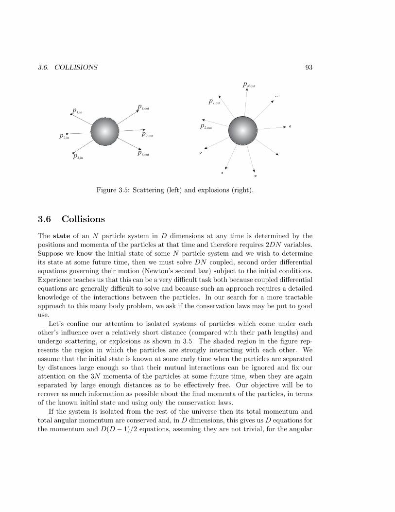
3.6. COLLISIONS 93
p1,in
p1,out
p1,out
p2,out
p2,out
p2,in
p3,in
p3,out
pN,out
Figure 3.5: Scattering (left) and explosions (right).
3.6 Collisions
The state of an N particle system in D dimensions at any time is determined by thepositions and momenta of the particles at that time and therefore requires 2DN variables.Suppose we know the initial state of some N particle system and we wish to determineits state at some future time, then we must solve DN coupled, second order differentialequations governing their motion (Newton’s second law) subject to the initial conditions.Experience teaches us that this can be a very difficult task both because coupled differentialequations are generally difficult to solve and because such an approach requires a detailedknowledge of the interactions between the particles. In our search for a more tractableapproach to this many body problem, we ask if the conservation laws may be put to gooduse.
Let’s confine our attention to isolated systems of particles which come under eachother’s influence over a relatively short distance (compared with their path lengths) andundergo scattering, or explosions as shown in 3.5. The shaded region in the figure rep-resents the region in which the particles are strongly interacting with each other. Weassume that the initial state is known at some early time when the particles are separatedby distances large enough so that their mutual interactions can be ignored and fix ourattention on the 3N momenta of the particles at some future time, when they are againseparated by large enough distances as to be effectively free. Our objective will be torecover as much information as possible about the final momenta of the particles, in termsof the known initial state and using only the conservation laws.
If the system is isolated from the rest of the universe then its total momentum andtotal angular momentum are conserved and, in D dimensions, this gives us D equations forthe momentum and D(D − 1)/2 equations, assuming they are not trivial, for the angular
94 CHAPTER 3. CONSERVATION THEOREMS
momentum, a total of D+D(D−1)/2 equations relating the particles’ initial positions andmomenta to their final positions and momenta. If, moreover, we have some informationabout the mechanical energy of the system (say, that the total mechanical energy, or somefraction of it, is preserved in the final state) then we have one additional condition, leadingto D +D(D − 1)/2 + 1 equations in all. We expect therefore that a direct application ofonly the conservation laws leaves ∆ = 2DN −D−D(D−1)/2−1 variables of the state ofthe system undetermined and conclude that if N is very large, conservation laws alone cantell us little about the evolution of the system – seeing that D is small. However, if N issmall the situation is different. For example, consider a system of two particles interactingin effectively one dimension. According to our formula, a straightforward application ofthe conservation laws would lead to ∆ = 2 undetermined variables. These variables wouldbe the final positions of the particles, so we are able to determine the final momenta ofthe particles without any a priori knowledge of the detailed force between them. For twoparticles in two effective dimensions, ∆ = 4 remain undetermined and these can onceagain be taken to represent the final positions of the two particles.
If we confine our attention to collisions in which the total angular momentum bothbefore and after the collision is identically zero, i.e., for which the angular momentumequations are in fact trivial, and ask only for the final momenta of the particles, we willhave at most D+1 conditions with which to determine DN final momenta. It follows thatthe problem of two particles colliding in effectively one dimension continues to be solvablewithout any a priori knowledge of the final state, whereas the collision of two particlesin two dimensions requires the knowledge of one final state variable and in D dimensionsrequires a knowledge of D−1 variables of the final state. Let us work out some illustrativeexamples.
3.6.1 One Dimensional Collisions
In a plastic or completely inelastic collision, energy is not conserved but the particlesstick together in the final state so that the number of momenta to be found is reducedto just the number of dimensions, D. Consider a plastic collision of two particles in onedimension. Let the particles have masses m1,2 and let their initial velocities be v1,i andv2,i respectively in some frame attached to the observer, which we’ll call the “Laboratoryframe”. The velocities (being vectors) are signed quantities in one dimension. As alwayswe will take velocities “to the right” to be positive and velocities “to the left” to benegative. As the particles stick together in the final state, there will be only one finalmomentum to be determined: that of the combination. The mass of the particle in theend state is m1 +m2 and we will call its velocity vf . Conservation of momentum impliesthat
m1v1i +m2v2i = (m1 +m2)vf (3.6.1)
3.6. COLLISIONS 95
and so
vf =m1v1i +m2v2i
(m1 +m2)(3.6.2)
solves the problem: the final velocity is simply the velocity the center of mass. Clearlymechanical energy was not conserved in this collision and we can determine the fractionof the initial mechanical energy that was lost,
Q =Kf
Ki=
(m1 +m2)v2f
m1v21i +m2v2
2i
. (3.6.3)
We find that
1−Q =m1m2(v1i − v2i)
2
(m1 +m2)(m1v21i +m2v2
2i)> 0 (3.6.4)
which shows that Q < 1. The lost mechanical energy is actually energy transferred to theenvironment as “heat” due to frictional forces during the collision, or as radiation if thecolliding particles were charged.
A slightly more difficult problem is that of an elastic collision in one dimension. Elasticcollisions conserve energy, so under the initial conditions of the system above we have twoequations (conservation of momentum and conservation of energy) that must be solvedfor the two final velocities,
m1v1i +m2v2i = m1v1f +m2v2f
1
2m1v
21i +
1
2m2v
22i =
1
2m1v
21f +
1
2m2v
22f (3.6.5)
Combining these two equations we find
v1i + v1f = v2i + v2f (3.6.6)
which serves to eliminate v2f (say). The result is5
v1f =m1 −m2
m1 +m2v1i +
2m2
m1 +m2v2i
v2f =m2 −m1
m1 +m2v2i +
2m1
m1 +m2v1i (3.6.7)
Two special cases are of interest: (a) If m1 = m2 = m then v1f = v2i and v2f = v1i i.e.,the particles simply exchange their velocities, and (b) if m2 m1 then v1f ' v1i andv2f ' 2v1i − v2i, i.e., the more massive particle simply moves as if it were unaffected bythe collision. In particular, if the more massive particle is at rest in the observer’s frame
5Problem: Fill in the omitted steps.
96 CHAPTER 3. CONSERVATION THEOREMS
then the smaller particle simply “bounces back”, v2f = −v2i. Alternatively, if the lighterparticle is initially at rest it will move at twice the speed of the larger particle after thecollision.
If the collision is not elastic, but the fraction of the initial mechanical energy that ispreserved in the final state is known to be Q ≤ 1 then the second equation of (3.6.5) ismodified to
m1v21f +m2v
22f = Q(m1v
21i +m2v
22i) (3.6.8)
and can once again be used, in combination with the conservation of momentum, to deter-mine the final velocities of the particles as above. The general expression is not particularlyilluminating and we leave this as an exercise to the interested reader.6 Collisions betweenmacroscopic bodies will always be inelastic and mechanical energy will be converted intoheat by frictional forces during the impact.
An important fact to note is that the result in (3.6.7) has the same form in anyreference frame. This can be shown directly by applying a Galilean transformation to theexpressions for v1,2f in the Laboratory frame. For a frame S′, traveling with a velocity v0
relative to the Laboratory frame, one has only to substitute
v′1i = v1i − v0, v′2i = v2i − v0,v′1f = v1f − v0, v′2f = v2f − v0, (3.6.9)
into (3.6.7) to obtain the expressions
v′1f =m1 −m2
m1 +m2v′1i +
2m2
m1 +m2v′2i
v′2f =m2 −m1
m1 +m2v′2i +
2m1
m1 +m2v′1i. (3.6.10)
Expressions that are form invariant under some set of transformations are said to becovariant under those transformations.
Now because the total momentum and angular momentum of the particles is conservedwhen there is no external force or torque on the system, the center of mass of the systemmust move with a constant velocity,
vcm =m1v1i +m2v2i
m1 +m2=m1v1f +m2v2f
m1 +m2, (3.6.11)
relative to the Laboratory frame. An observer who is attached to the center of massand moves along with it is therefore inertial, so what would a collision look like from herpoint of view? Since the total momentum in this frame must be zero, the conservation ofmomentum implies that
m1v′1i +m2v
′2i = 0 = m1v
′1f +m2v
′2f ⇒ v′2i = −m1
m2v′1i, v′2f = −m1
m2v′1f . (3.6.12)
6Problem: Determine the final velocities in terms of the initial velocities and the fraction Q.
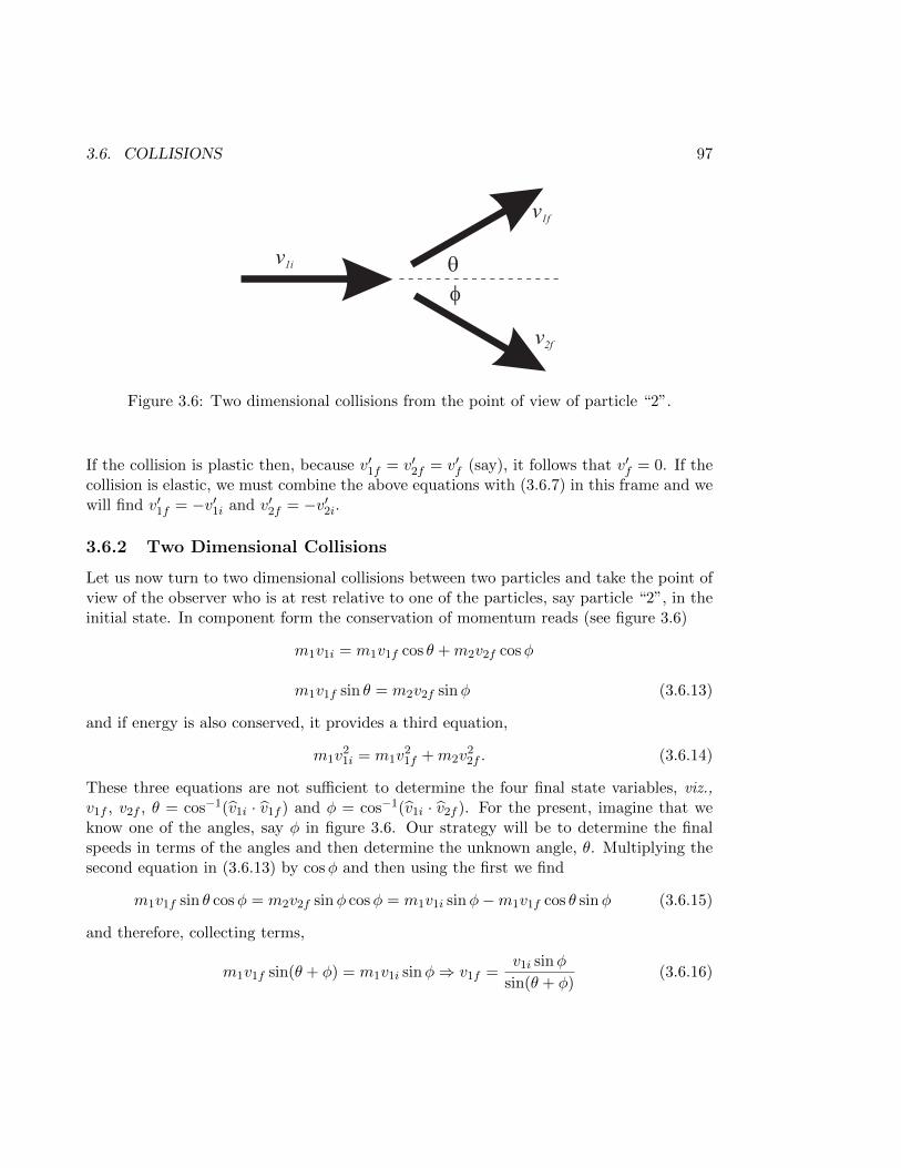
3.6. COLLISIONS 97
q
f
v1i
v1f
v2f
Figure 3.6: Two dimensional collisions from the point of view of particle “2”.
If the collision is plastic then, because v′1f = v′2f = v′f (say), it follows that v′f = 0. If thecollision is elastic, we must combine the above equations with (3.6.7) in this frame and wewill find v′1f = −v′1i and v′2f = −v′2i.
3.6.2 Two Dimensional Collisions
Let us now turn to two dimensional collisions between two particles and take the point ofview of the observer who is at rest relative to one of the particles, say particle “2”, in theinitial state. In component form the conservation of momentum reads (see figure 3.6)
m1v1i = m1v1f cos θ +m2v2f cosφ
m1v1f sin θ = m2v2f sinφ (3.6.13)
and if energy is also conserved, it provides a third equation,
m1v21i = m1v
21f +m2v
22f . (3.6.14)
These three equations are not sufficient to determine the four final state variables, viz.,v1f , v2f , θ = cos−1(v1i · v1f ) and φ = cos−1(v1i · v2f ). For the present, imagine that weknow one of the angles, say φ in figure 3.6. Our strategy will be to determine the finalspeeds in terms of the angles and then determine the unknown angle, θ. Multiplying thesecond equation in (3.6.13) by cosφ and then using the first we find
m1v1f sin θ cosφ = m2v2f sinφ cosφ = m1v1i sinφ−m1v1f cos θ sinφ (3.6.15)
and therefore, collecting terms,
m1v1f sin(θ + φ) = m1v1i sinφ⇒ v1f =v1i sinφ
sin(θ + φ)(3.6.16)
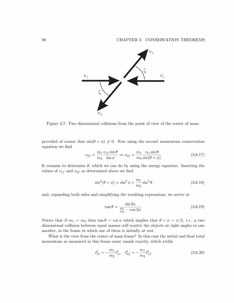
98 CHAPTER 3. CONSERVATION THEOREMS
z
z
v1i v2i
v1f
v2f
Figure 3.7: Two dimensional collisions from the point of view of the center of mass.
provided of course that sin(θ + φ) 6= 0. Now using the second momentum conservationequation we find
v2f =m1
m2
v1f sin θ
sinφ⇒ v2f =
m1
m2
v1i sin θ
sin(θ + φ)(3.6.17)
It remains to determine θ, which we can do by using the energy equation. Inserting thevalues of v1f and v2f as determined above we find
sin2(θ + φ) = sin2 φ+m1
m2sin2 θ (3.6.18)
and, expanding both sides and simplifying the resulting expressions, we arrive at
tan θ =sin 2φ
m1m2− cos 2φ
. (3.6.19)
Notice that if m1 = m2 then tan θ = cotφ which implies that θ + φ = π/2, i.e., a twodimensional collision between equal masses will scatter the objects at right angles to oneanother, in the frame in which one of them is initially at rest.
What is the view from the center of mass frame? In this case the initial and final totalmomentum as measured in this frame must vanish exactly, which yields
~v′2i = −m1
m2~v′1i, ~v′2f = −m1
m2~v′1f (3.6.20)
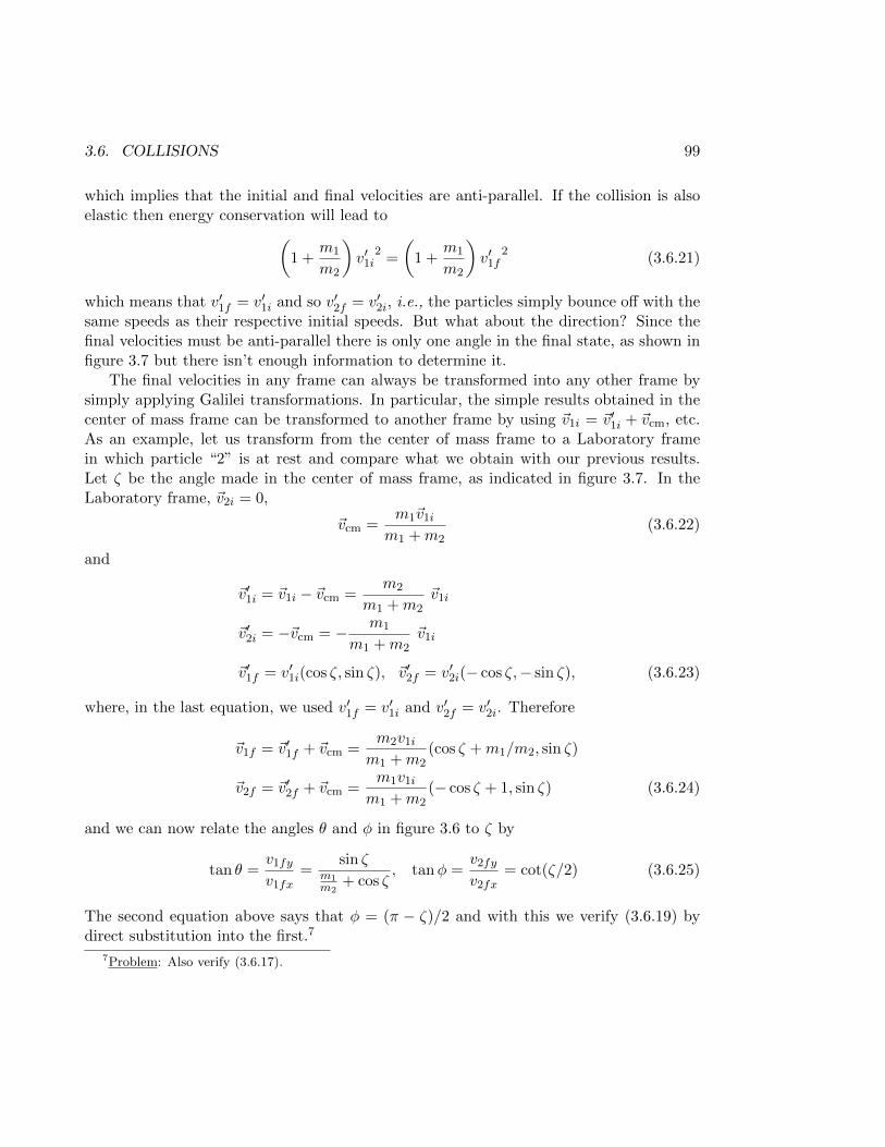
3.6. COLLISIONS 99
which implies that the initial and final velocities are anti-parallel. If the collision is alsoelastic then energy conservation will lead to(
1 +m1
m2
)v′1i
2=
(1 +
m1
m2
)v′1f
2(3.6.21)
which means that v′1f = v′1i and so v′2f = v′2i, i.e., the particles simply bounce off with thesame speeds as their respective initial speeds. But what about the direction? Since thefinal velocities must be anti-parallel there is only one angle in the final state, as shown infigure 3.7 but there isn’t enough information to determine it.
The final velocities in any frame can always be transformed into any other frame bysimply applying Galilei transformations. In particular, the simple results obtained in thecenter of mass frame can be transformed to another frame by using ~v1i = ~v′1i + ~vcm, etc.As an example, let us transform from the center of mass frame to a Laboratory framein which particle “2” is at rest and compare what we obtain with our previous results.Let ζ be the angle made in the center of mass frame, as indicated in figure 3.7. In theLaboratory frame, ~v2i = 0,
~vcm =m1~v1i
m1 +m2(3.6.22)
and
~v′1i = ~v1i − ~vcm =m2
m1 +m2~v1i
~v′2i = −~vcm = − m1
m1 +m2~v1i
~v′1f = v′1i(cos ζ, sin ζ), ~v′2f = v′2i(− cos ζ,− sin ζ), (3.6.23)
where, in the last equation, we used v′1f = v′1i and v′2f = v′2i. Therefore
~v1f = ~v′1f + ~vcm =m2v1i
m1 +m2(cos ζ +m1/m2, sin ζ)
~v2f = ~v′2f + ~vcm =m1v1i
m1 +m2(− cos ζ + 1, sin ζ) (3.6.24)
and we can now relate the angles θ and φ in figure 3.6 to ζ by
tan θ =v1fy
v1fx=
sin ζm1m2
+ cos ζ, tanφ =
v2fy
v2fx= cot(ζ/2) (3.6.25)
The second equation above says that φ = (π − ζ)/2 and with this we verify (3.6.19) bydirect substitution into the first.7
7Problem: Also verify (3.6.17).
100 CHAPTER 3. CONSERVATION THEOREMS
3.7 The Virial Theorem
The virial theorem relates the average kinetic energy of the particles of a many bodysystem to the so-called virial, which is closely related to their average potential energyin cases of physical interest. Consider a system of particles which have momenta ~pn andpositions ~rn and define the quantity
S =∑n
~rn · ~pn (3.7.1)
then the rate of change of S is given by
dS
dt=∑n
(~rn · ~pn + ~rn · ~pn) (3.7.2)
Consider the average rate of change,⟨dS
dt
⟩τ
= 〈∑n
~rn · ~pn〉τ + 〈∑n
~rn · ~pn〉τ (3.7.3)
where the average is defined over some time interval, say [0, τ ], in the usual way,⟨dS
dt
⟩τ
=1
τ
∫ τ
0dtdS
dt=
1
τ
∫ τ
0dS(t). (3.7.4)
By definition then, ⟨dS
dτ
⟩τ
=S(τ)− S(0)
τ. (3.7.5)
If the mechanical state of the system is periodic, i.e., the particles of the system returnto their positions and momenta at t = 0 after an interval an interval of time τ , then itfollows that ⟨
dS
dt
⟩τ
= 0 (3.7.6)
On he other hand, if the motion is not periodic, assume that neither the positions nor themomenta ever approach infinity during the evolution of the system. This makes sense ifthe system is bound, and as a consequence S(τ) − S(0) is always finite. If we considervery large times, taking τ →∞, then clearly
limτ→∞
⟨dS
dt
⟩τ
→ 0 (3.7.7)
But this means that over the time interval τ (one period for periodic systems and infinitefor systems that are not periodic but bounded)∑
n
〈~rn · ~pn〉τ = −∑n
〈~rn · ~pn〉τ (3.7.8)
3.7. THE VIRIAL THEOREM 101
Now ~Fn = ~pn and ~pn · ~rn = 2Kn. Therefore the left hand side of the equation is twice thetime averaged kinetic energy and we have
〈K〉τ = −1
2〈∑n
~rn · ~Fn〉τ (3.7.9)
The average on the right hand side is called the Virial, and the relationship betweenthe time averaged kinetic energy and the Virial is called the Virial Theorem. Now ~Fnrepresents the total force on the particle labeled n. If all the forces, internal and externalare conservative, so is ~Fn and we can write
~Fn = −~∇nUn. (3.7.10)
The time averaged kinetic energy becomes
〈K〉τ =1
2〈∑n
~rn · ~∇nUn〉τ (3.7.11)
To understand its significance, consider what this means for a bound, self-gravitatingsystem of particles such as, say, a galaxy or even a group of galaxies (stars are smallcompared to the distance between them and may be considered particles over galacticscales). Thus we have to consider only the internal potential energies of interactions, so
1
2
∑n
~rn · ~∇nUn =1
2
∑n,m 6=n
~rn · ~∇nUnm(|~rn − ~rm|)
=1
4
∑n,m 6=n
(~rn − ~rm) · ~∇nUnm(|~rn − ~rm|) (3.7.12)
where we have used ~∇nUnm = −~∇mUmn. Now suppose that
Unm(|~rn − ~rm|) = knm|~rn − ~rm|α+1 (3.7.13)
where knm is a constant depending on the properties of particles m and n and α 6= −1.For instance, if the interactions are purely gravitational, kmn = −GMnMm where Mn andMm are the masses of particles n and m respectively and α = −2. We find
(~rn − ~rm) · ~∇nUnm = (α+ 1)Unm (3.7.14)
and so, using
U int =1
2
∑n,m 6=n
Unm, (3.7.15)
102 CHAPTER 3. CONSERVATION THEOREMS
we find that
〈K〉τ =1
2〈∑n
~rn · ~∇nUn〉τ =α+ 1
2〈U int〉τ . (3.7.16)
In particular, when α = −2 the time averaged kinetic energy is precisely minus one half ofthe time averaged potential energy of the system!8 On the other hand, the time averagedkinetic energy is precisely equal to the time averaged potential energy of a harmonicoscillator.
8Problem: Determine the Virial for the the Yukawa interaction,
Unm(|~rn − ~rm|) =knm
|~rn − ~rm|e−α|~rn−~rm|
where α is independent of m,n.
Chapter 4
Newtonian Gravity
We have seen that once the dependence of a force on the position, velocity and timehas been experimentally determined then the problem of calculating the trajectory of aparticle under the influence of the force is a mathematical problem of fundamental interest.If an exact solution is obtained there are usually two free parameters per space dimension,which can be thought of as representing the initial position and velocity of the particle.Sometimes, a more fruitful way to think about these constants is in terms of conservedquantities. The allowed motions can then be classified by these conserved quantities. Weshall soon see how this comes about, but first let us examine the gravitational force ingreater detail.
4.1 The force law
Gravitation was the first of the fundamental forces to be discovered and for which a“force law” was given. The force law was first given by Newton after many years ofstudying Kepler’s (1571-1630) three laws of planetary motion and Tyco Brahe’s (1546-1601) excellent observational data on the same.1 We have already mentioned Newton’slaw of gravitation before. It says simply that the force of attraction exerted by a body ofmass m1 on another of mass m2 located respectively at ~r1 and ~r2 is given by
~F1→2 = −G m1m2
|~r2 − ~r1|3(~r2 − ~r1) (4.1.1)
This force is always attractive because mass is positive.
A most remarkable fact about the gravitational force is that it depends on the massesof the particles, in the same way as the electromagnetic force depends on the charges. m1
1 Kepler was initially Tycho Brahe’s assistant and carried on his work after Tycho Brahe’s death in1601.
103
104 CHAPTER 4. NEWTONIAN GRAVITY
and m2 can therefore be thought of as gravitational “charges” and there is no a priorireason to expect that they are precisely the inertial masses of the particles, i.e., the massesthat appear on the left hand side of Newton’s second law of motion. Experimentally,however, one finds that they the gravitational mass and the inertial mass are identical upto about one part in 1011 and it is necessary therefore to assume this as a principle. Thesimple statement that gravitational and inertial masses are the same is called the “weakequivalence principle”. A stronger form of the equivalence principle was given by Einsteinin making the transition from Newtonian gravity, summarized by the weak equivalenceprinciple and (4.1.1), and General Relativity, which is a theory about non-inertial frames.
As a consequence of the weak equivalence principle, the equations of motion for aparticle, say particle 2, do not involve its inertia,
d2~r2
dt2= −Gm1
r212
r12 = ~g(~r2) (4.1.2)
where ~r12 = ~r2 − ~r1 and ~g(~r) denotes the gravitational acceleration. One could evenconclude that gravity is not a force in the traditional Newtonian sense, since motionunder its influence is kinematical: when a gravitational field is present, the kinematicalequation
d2~r
dt2= 0 (4.1.3)
should be replaced by the more general
d2~r
dt2= ~g(~r) (4.1.4)
where ~g(~r) would be a property of the space(time) in which the particle is moving. Thiskinematical equation would not lead to “motion in a straight line with constant velocity”,as required by Newton’s first law of motion. However, the “straight line” can be thoughtof as the shortest distance between two points in a flat space(time), so the presence ofmatter (more generally, energy) in space must bend the space(time) in its neighborhood,causing the shortest distance between two points to no longer be a straight line.2 Particletrajectories between two points would then be geodesics, not necessarily straight lines.General Relativity is a theory of how space(time) is curved by the presence of matter(energy). We will ignore this modified view of gravity and take the Newtonian approach,treating gravity as a force. It is a very good approximation as long as the gravitationalforce is weak and the speeds involved are small compared with the speed of light. Thegravitational acceleration, ~g(~r) is called the “gravitational field vector”. It can be defined,for an arbitrary distribution of matter by two equations, which we now examine.
2Trajectories that minimize the distance between two points are called geodesics.
4.2. TWO PROPERTIES OF THE GRAVITATIONAL FIELD 105
4.2 Two properties of the gravitational field
Suppose we have a distribution of point particles, each labeled by an integer n, locatedat ~rn and having a mass mn. Consider a test particle of mass M and located at ~r in theneighborhood of this distribution. Assuming that the net force on the test body is thesum of forces exerted by each of the particles in the distribution on it, we have
~F = −GN∑n=1
Mmn(~r − ~rn)
|~r − ~rn|3(4.2.1)
This would give the gravitational acceleration of our test body (also known as the gravi-tational field vector) at the point ~r as
~g(~r) = −GN∑n=1
mn(~r − ~rn)
|~r − ~rn|3(4.2.2)
If the distribution can be considered continuous (this means that the average separationbetween the atoms/molecules that make up the system is on the order of the typicalatomic/molecular size), then we can divide the system into infinitesimal pieces, each ofmass dm(~r′) and add up the contribution of each infinitesimal mass to the gravitationalfield vector at ~r as we did before, except that now the sum is continuous and not discrete,i.e., it becomes an integral over distribution,
~g(~r) = −G∫Ddm(~r′)
(~r − ~r′)|~r − ~r′|3
(4.2.3)
We can express the mass of the infinitesimal pieces in terms of the density of the distri-bution: dm(~r′) = ρ(~r′)d3~r′ and reexpress the field vector as a volume integral over thedistribution,
~g(~r) = −G∫VD
d3~r′ρ(~r′)(~r − ~r′)|~r − ~r′|3
(4.2.4)
We have made a rather important assumption in all of the above: we assumed that thegravitational force on a body due to a distribution is the simple sum of forces exerted on itby elements of the distribution. In other words, the interaction between an pair of bodiesdoes not affect the interaction of any of the bodies in the pair and a third body in theirneighborhood. This assumption fails in general relativity, which is a non-linear theory ofthe gravitational field. If the field is sufficiently weak, however, superposition of forces isa very good approximation.
It is easy to see from (4.1.2) that the gravitational field vector due to a single massivebody satisfies
~∇× ~g = 0 (4.2.5)
106 CHAPTER 4. NEWTONIAN GRAVITY
This can be proved by simply taking the curl of the left hand side of (4.1.2). Of course itwill hold for the gravitational field vector of a distribution too as long as the resulting ~g(~r)is obtained by simply adding the contributions from elementary masses in the distribution(superposition). Thus, for the field vector due to a point mass, m, located at ~r′,
~∇× ~g = −Gm~∇× (~r − ~r′)|~r − ~r′|3
= −Gm
[~∇× (~r − ~r′)|~r − ~r′|3
− (~r − ~r′)× ~∇ 1
|~r − ~r′|3
](4.2.6)
Now
[~∇× (~r − ~r′)]i = εijk∂j(xk − x′k) = εijkδjk ≡ 0 (4.2.7)
by the antisymmetry of the Levi-Civita symbol, and
[~∇ 1
|~r − ~r′|3
]i
= ∂i
∑j
(xj − x′j)2
−3/2
= −3
∑j
(xj − x′j)2
−5/2
(xj − x′j)δij
= −[
3(~r − ~r′)|~r − ~r′|5
]i
(4.2.8)
so
~∇× ~g = −3Gm(~r − ~r′)× (~r − ~r′)|~r − ~r′|5
= 0. (4.2.9)
Because ~g is irrotational it can be expressed as the gradient of a scalar function and wecan write
~g = −~∇φ (4.2.10)
(the minus sign is inserted for later convenience). The scalar function φ is called thegravitational potential. The gravitational field has not three but just one (continuous)degree of freedom since all of the three components of ~g are obtained from the gradient ofa single scalar field. Knowing ~g we can determine φ: for a point particle, of mass m,
φ(~r) = − Gm
|~r − ~r′|(4.2.11)
and, because we can superpose the gravitational field (at least, in the Newtonian approx-imation), we can also superpose the gravitational potential. It follows that for a discretedistribution, made up of masses mn located at ~rn,
φ(~r) = −G∑n
mn
|~r − ~rn|(4.2.12)
4.2. TWO PROPERTIES OF THE GRAVITATIONAL FIELD 107
and for a continuous distribution characterized by the density ρ(~r),
φ(~r) = −G∫VD
d3~r′ρ(~r′)
|~r − ~r′|(4.2.13)
The gravitational force on a mass M located in the neighborhood of the distribution canbe expressed in terms of the gravitational potential,
~F = M~g = −M~∇φ (4.2.14)
The gravitational force is obviously conservative. This means that we can define thepotential energy of a body of mass M in the neighborhood of a distribution of masses as
UM (~r) = −∫ ~r
∗~F · d~r = M
∫ ~r
∗~∇φ · d~r = M [φ(~r)− φ(∗)] (4.2.15)
where ∗ is used to represent the standard fixed point to which the potential energy isreferred.
A second property of the gravitational field,
~∇ · ~g = −4πGρ (4.2.16)
follows from Gauss’ theorem. Again, if we can prove this for a point mass, then it willhold true for arbitrary mass distributions, simply because of superposition. Consider aclosed surface, S and let us begin by evaluating∮
SdS n · ~g = −Gm
∮SdS
n · (~r − ~r′)|~r − ~r′|3
= −Gm∮SdS
cos θ
|~r − ~r′|2(4.2.17)
where θ is the angle between the normal to the surface and the outward radial vector fromthe charge. Now dS n · (~r − ~r′)/|~r − ~r′| is just the projection of the surface area dS onthe sphere of radius |~r − ~r′|, therefore the integrand is simply the solid angle subtendedby the projection of dS on the sphere of that radius at the charge q. If we sum up theseinfinitesimal solid angles, then two cases may arise: (a) the original surface S does notenclose the mass m (see figure(4.1)), or (b) the mass is enclosed by the surface S (see figure(4.2)). In case (a), the net result of summing up the solid angles subtended at m will beidentically zero due to the two equal and opposite contributions from region I, where cos θis negative, and from region II, where cos θ is positive. The contribution from region I isnegative, whereas the contribution from region II is positive and equal in magnitude tothe contribution from region I. In case (b), the infinitesimal solid angles add up to giveprecisely the total solid angle of 4π. Thus we find that∮
SdS n · ~g = −4πGmin (4.2.18)
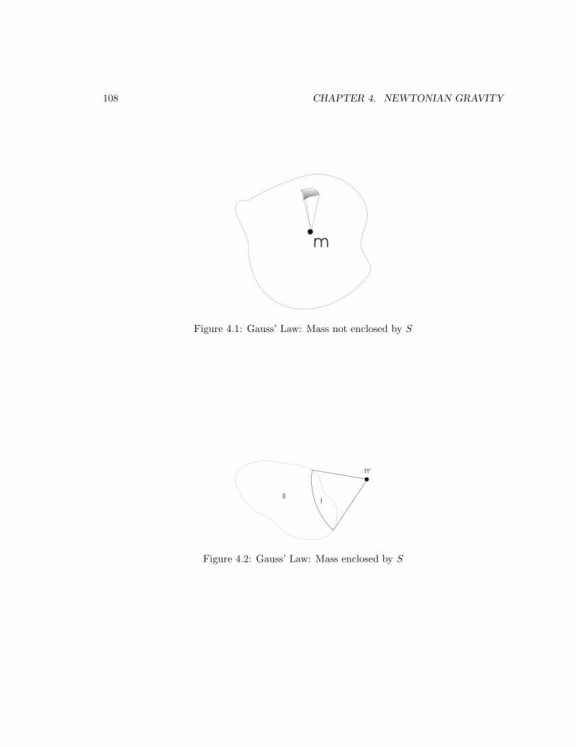
108 CHAPTER 4. NEWTONIAN GRAVITY
Figure 4.1: Gauss’ Law: Mass not enclosed by S
Figure 4.2: Gauss’ Law: Mass enclosed by S
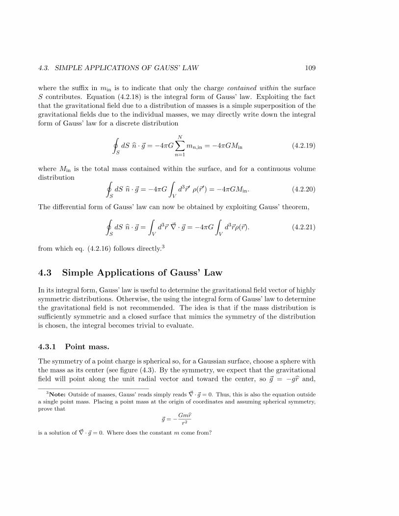
4.3. SIMPLE APPLICATIONS OF GAUSS’ LAW 109
where the suffix in min is to indicate that only the charge contained within the surfaceS contributes. Equation (4.2.18) is the integral form of Gauss’ law. Exploiting the factthat the gravitational field due to a distribution of masses is a simple superposition of thegravitational fields due to the individual masses, we may directly write down the integralform of Gauss’ law for a discrete distribution∮
SdS n · ~g = −4πG
N∑n=1
mn,in = −4πGMin (4.2.19)
where Min is the total mass contained within the surface, and for a continuous volumedistribution ∮
SdS n · ~g = −4πG
∫Vd3~r′ ρ(~r′) = −4πGMin. (4.2.20)
The differential form of Gauss’ law can now be obtained by exploiting Gauss’ theorem,∮SdS n · ~g =
∫Vd3~r ~∇ · ~g = −4πG
∫Vd3~rρ(~r). (4.2.21)
from which eq. (4.2.16) follows directly.3
4.3 Simple Applications of Gauss’ Law
In its integral form, Gauss’ law is useful to determine the gravitational field vector of highlysymmetric distributions. Otherwise, the using the integral form of Gauss’ law to determinethe gravitational field is not recommended. The idea is that if the mass distribution issufficiently symmetric and a closed surface that mimics the symmetry of the distributionis chosen, the integral becomes trivial to evaluate.
4.3.1 Point mass.
The symmetry of a point charge is spherical so, for a Gaussian surface, choose a sphere withthe mass as its center (see figure (4.3). By the symmetry, we expect that the gravitationalfield will point along the unit radial vector and toward the center, so ~g = −gr and,
3Note: Outside of masses, Gauss’ reads simply reads ~∇ ·~g = 0. Thus, this is also the equation outsidea single point mass. Placing a point mass at the origin of coordinates and assuming spherical symmetry,prove that
~g = −Gmrr2
is a solution of ~∇ · ~g = 0. Where does the constant m come from?
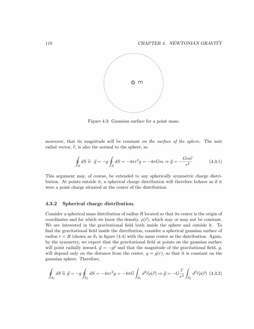
110 CHAPTER 4. NEWTONIAN GRAVITY
Figure 4.3: Gaussian surface for a point mass.
moreover, that its magnitude will be constant on the surface of the sphere. The unitradial vector, r, is also the normal to the sphere, so∮
SdS n · ~g = −g
∮SdS = −4πr2g = −4πGm⇒ ~g = −Gmr
r2(4.3.1)
This argument may, of course, be extended to any spherically symmetric charge distri-bution. At points outside it, a spherical charge distribution will therefore behave as if itwere a point charge situated at the center of the distribution.
4.3.2 Spherical charge distribution.
Consider a spherical mass distribution of radius R located so that its center is the origin ofcoordinates and for which we know the density, ρ(~r), which may or may not be constant.We are interested in the gravitational field both inside the sphere and outside it. Tofind the gravitational field inside the distribution, consider a spherical gaussian surface ofradius r < R (shown as S1 in figure (4.4) with the same center as the distribution. Again,by the symmetry, we expect that the gravitational field at points on the gaussian surfacewill point radially inward, ~g = −gr and that the magnitude of the gravitational field, g,will depend only on the distance from the center, g = g(r), so that it is constant on thegaussian sphere. Therefore,∮
S1
dS n ·~g = −g∮S1
dS = −4πr2g = −4πG
∫S1
d3~rρ(~r)⇒ ~g = −G r
r2
∫S1
d3~rρ(~r) (4.3.2)
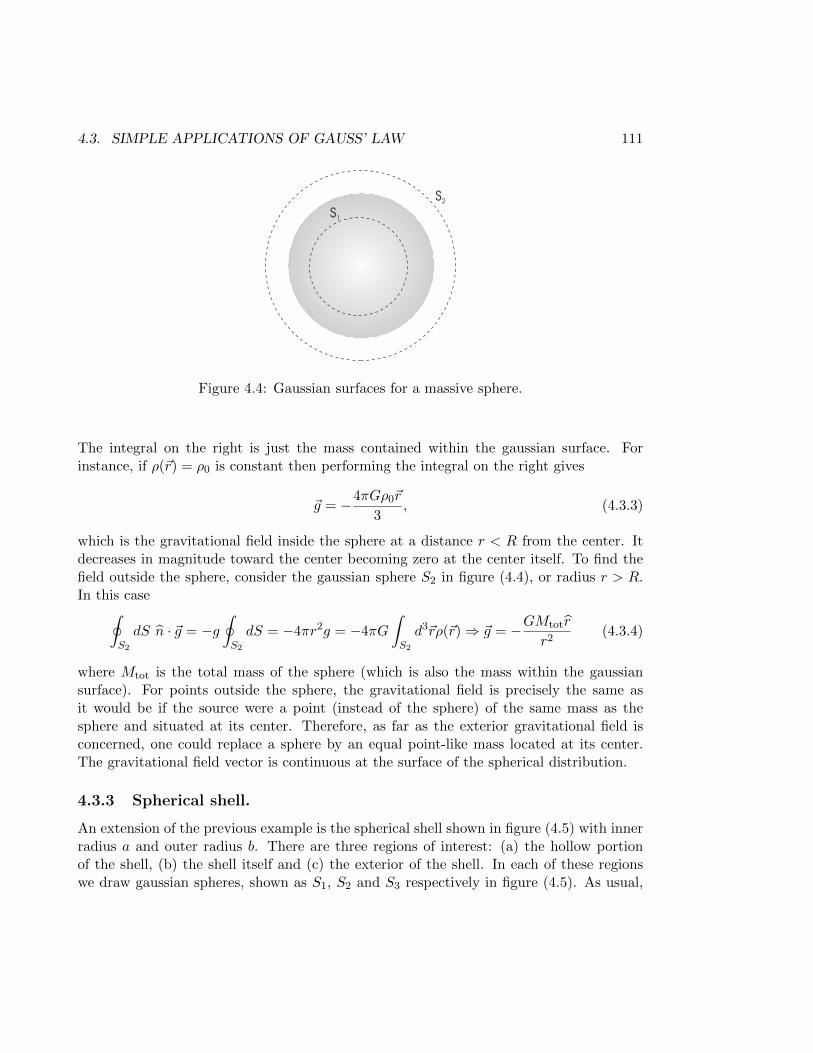
4.3. SIMPLE APPLICATIONS OF GAUSS’ LAW 111
Figure 4.4: Gaussian surfaces for a massive sphere.
The integral on the right is just the mass contained within the gaussian surface. Forinstance, if ρ(~r) = ρ0 is constant then performing the integral on the right gives
~g = −4πGρ0~r
3, (4.3.3)
which is the gravitational field inside the sphere at a distance r < R from the center. Itdecreases in magnitude toward the center becoming zero at the center itself. To find thefield outside the sphere, consider the gaussian sphere S2 in figure (4.4), or radius r > R.In this case∮
S2
dS n · ~g = −g∮S2
dS = −4πr2g = −4πG
∫S2
d3~rρ(~r)⇒ ~g = −GMtotr
r2(4.3.4)
where Mtot is the total mass of the sphere (which is also the mass within the gaussiansurface). For points outside the sphere, the gravitational field is precisely the same asit would be if the source were a point (instead of the sphere) of the same mass as thesphere and situated at its center. Therefore, as far as the exterior gravitational field isconcerned, one could replace a sphere by an equal point-like mass located at its center.The gravitational field vector is continuous at the surface of the spherical distribution.
4.3.3 Spherical shell.
An extension of the previous example is the spherical shell shown in figure (4.5) with innerradius a and outer radius b. There are three regions of interest: (a) the hollow portionof the shell, (b) the shell itself and (c) the exterior of the shell. In each of these regionswe draw gaussian spheres, shown as S1, S2 and S3 respectively in figure (4.5). As usual,
112 CHAPTER 4. NEWTONIAN GRAVITY
Figure 4.5: Gaussian surfaces for a massive spherical shell.
spherical symmetry implies that the gravitational field is directed radially inward and thatits magnitude depends only on the distance from the center. Therefore, inside the hollowportion (r < a) and on the gaussian sphere S1,∮
S1
dS n · ~g = −g∮S1
dS = −4πr2g = −4πG
∫S1
d3~rρ(~r) = 0⇒ ~g = 0 (4.3.5)
i.e., the gravitational field vanishes at all points here. Inside the shell itself (a < r < b),∮S2
dS n ·~g = −g∮S2
dS = −4πr2g = −4πG
∫S2
d3~rρ(~r)⇒ ~g = −G r
r2
∫S2
d3~rρ(~r) (4.3.6)
If the density is constant
~g = −4πGρ0r
r2(r3 − a3) (4.3.7)
Outside the shell (r > b) an argument similar to the one we made for the sphere tells usthat
~g = −GMtotr
r2(4.3.8)
where Mtot is the total mass of the shell.
4.3.4 Infinite line of constant linear mass density (cosmic string).
The symmetry of an infinite line of mass (infinite string) is that of a right circular cylinder.For a Gaussian surface, choose an infinite cylinder with the line of charge along its axis(see figure (4.6).
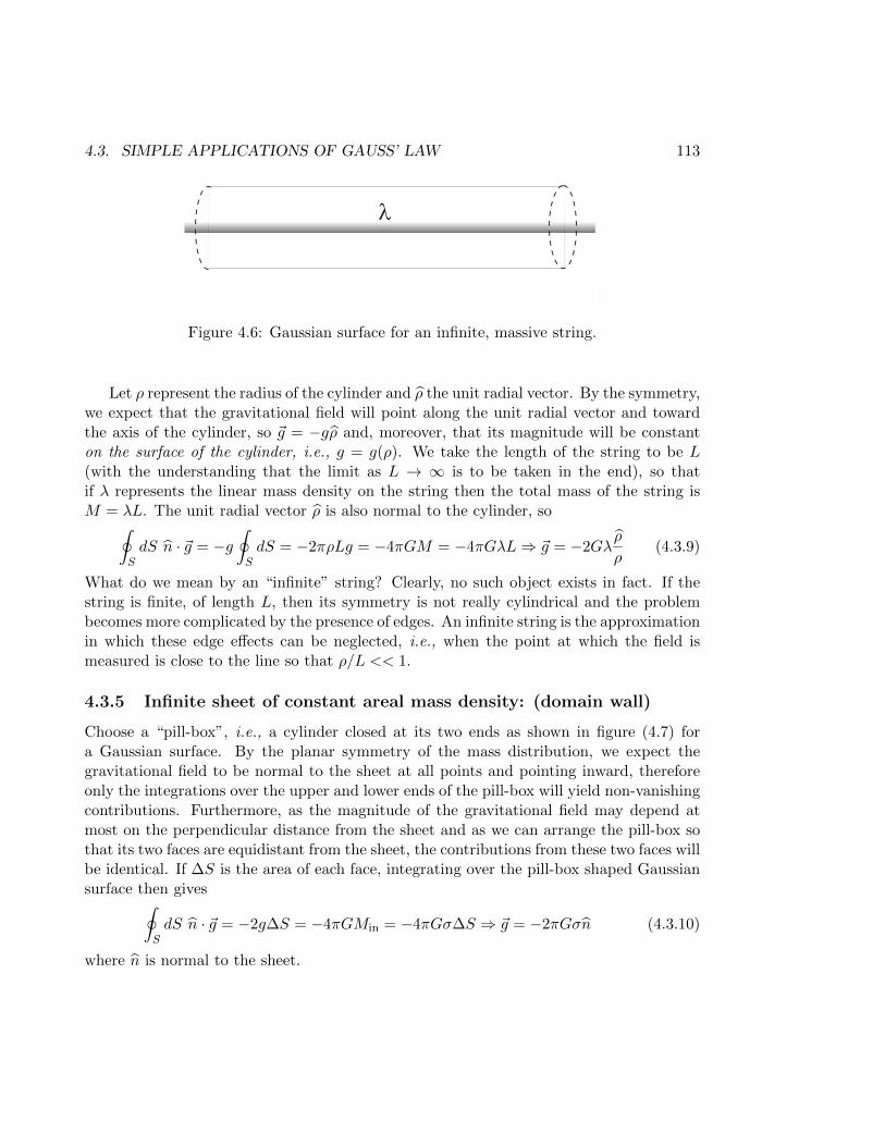
4.3. SIMPLE APPLICATIONS OF GAUSS’ LAW 113
Figure 4.6: Gaussian surface for an infinite, massive string.
Let ρ represent the radius of the cylinder and ρ the unit radial vector. By the symmetry,we expect that the gravitational field will point along the unit radial vector and towardthe axis of the cylinder, so ~g = −gρ and, moreover, that its magnitude will be constanton the surface of the cylinder, i.e., g = g(ρ). We take the length of the string to be L(with the understanding that the limit as L → ∞ is to be taken in the end), so thatif λ represents the linear mass density on the string then the total mass of the string isM = λL. The unit radial vector ρ is also normal to the cylinder, so∮
SdS n · ~g = −g
∮SdS = −2πρLg = −4πGM = −4πGλL⇒ ~g = −2Gλ
ρ
ρ(4.3.9)
What do we mean by an “infinite” string? Clearly, no such object exists in fact. If thestring is finite, of length L, then its symmetry is not really cylindrical and the problembecomes more complicated by the presence of edges. An infinite string is the approximationin which these edge effects can be neglected, i.e., when the point at which the field ismeasured is close to the line so that ρ/L << 1.
4.3.5 Infinite sheet of constant areal mass density: (domain wall)
Choose a “pill-box”, i.e., a cylinder closed at its two ends as shown in figure (4.7) fora Gaussian surface. By the planar symmetry of the mass distribution, we expect thegravitational field to be normal to the sheet at all points and pointing inward, thereforeonly the integrations over the upper and lower ends of the pill-box will yield non-vanishingcontributions. Furthermore, as the magnitude of the gravitational field may depend atmost on the perpendicular distance from the sheet and as we can arrange the pill-box sothat its two faces are equidistant from the sheet, the contributions from these two faces willbe identical. If ∆S is the area of each face, integrating over the pill-box shaped Gaussiansurface then gives∮
SdS n · ~g = −2g∆S = −4πGMin = −4πGσ∆S ⇒ ~g = −2πGσn (4.3.10)
where n is normal to the sheet.
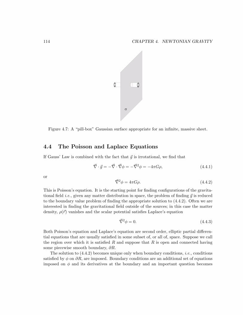
114 CHAPTER 4. NEWTONIAN GRAVITY
Figure 4.7: A “pill-box” Gaussian surface appropriate for an infinite, massive sheet.
4.4 The Poisson and Laplace Equations
If Gauss’ Law is combined with the fact that ~g is irrotational, we find that
~∇ · ~g = −~∇ · ~∇φ = −~∇2φ = −4πGρ, (4.4.1)
or~∇2φ = 4πGρ. (4.4.2)
This is Poisson’s equation. It is the starting point for finding configurations of the gravita-tional field i.e., given any matter distribution in space, the problem of finding ~g is reducedto the boundary value problem of finding the appropriate solution to (4.4.2). Often we areinterested in finding the gravitational field outside of the sources; in this case the matterdensity, ρ(~r) vanishes and the scalar potential satisfies Laplace’s equation
~∇2φ = 0. (4.4.3)
Both Poisson’s equation and Laplace’s equation are second order, elliptic partial differen-tial equations that are usually satisfied in some subset of, or all of, space. Suppose we callthe region over which it is satisfied R and suppose that R is open and connected havingsome piecewise smooth boundary, ∂R.
The solution to (4.4.2) becomes unique only when boundary conditions, i.e., conditionssatisfied by φ on ∂R, are imposed. Boundary conditions are an additional set of equationsimposed on φ and its derivatives at the boundary and an important question becomes
4.4. THE POISSON AND LAPLACE EQUATIONS 115
what boundary conditions are required to have a unique solution to a given problem. Ingeneral, in order to obtain a unique solution to any partial differential equation of orderk in n dimensions, one requires to specify the function and k − 1 normal derivatives ofthe function on ∂R. These are the Cauchy conditions (sometimes referred to as Cauchy“data”). Thus, typically two kinds of boundary conditions ensure unique solutions ofPoisson’s equation:
• the Dirichlet condition specifies the value of φ(~r) on ∂R and
• the Neumann condition specifies the normal derivative, n · ~∇φ(~r), on the boundary,where n is the unit normal to ∂R.
In practice, however, either one or the other may suffice to completely determine theunique solution.
If there are no non-trivial boundaries, the gravitational potential is generally requiredto fall off to zero at infinity and the solution can be no different from the solution we havealready obtained,
φ(~r) = −G∫VD
d3~r′ρ(~r′)
|~r − ~r′|, (4.4.4)
where the integration is performed over the charge distribution D. But this means thatthe right hand side of the above equation should obey (4.4.2). Taking the Laplacian ofthe solution gives
~∇2φ = −G∫VD
d3~r′ρ(~r′)~∇2 1
|~r − ~r′|(4.4.5)
and we see that
~∇2 1
|~r − ~r′|= ∂i
xi − x′i|~r − ~r′|3
= 0, (4.4.6)
provided that ~r 6= ~r′. However, it is badly defined at ~r = ~r′ and this is precisely the limitthat supports the integral above to give a non-zero right hand side. We thus encounterthe three dimensional version of the “δ−function”, introduced in the previous chapter. Ifwe call
~∇2 1
|~r − ~r′|= −4πδ3(~r − ~r′), (4.4.7)
then, because~∇2φ(~r) = 4πGρ(~r), (4.4.8)
the distribution δ3(~r − ~r′) must have the following property∫d3~r′f(~r′)δ3(~r − ~r′) = f(~r) (4.4.9)
116 CHAPTER 4. NEWTONIAN GRAVITY
for any function, f(~r). In particular, taking f(~r′) = 1, we should have∫d3~r′δ(~r − ~r′) = 1 (4.4.10)
In the parlance of the previous chapter,
G(~r − ~r′) = − 1
4π|~r − ~r′|(4.4.11)
is the Green’s function of the Laplacian.4
We can convince ourselves of (4.4.7) by applying Gauss’ theorem,
− 1
4π
∫d3~r ~∇2
(1
r
)= − 1
4π
∮Sd~S · ~∇
(1
r
)(4.4.12)
where S is a closed surface bounding the region of integration. Clearly, only the radialcomponent of the surface normal will contribute to the integral. In other words, given anyarbitrary bounding surface, only the projection of this surface on a sphere of radius r isrelevant. This means that, without loss of generality, we can take S to be a sphere andwrite the integral as
− 1
4π
∮Sd~S · ~∇
(1
r
)=
1
4π
∮Sdθdφr2
(1
r2
)= 1 (4.4.13)
as required.Naturally, the Green’s function in (4.4.11) is only defined up to the addition of an
arbtrary solution of Laplace’s equation, i.e., more generally G(~r − ~r′) can be written as
G(~r − ~r′) = − 1
4π|~r − ~r′|+Q(~r − ~r′) (4.4.14)
where ~∇2Q(~r − ~r′) = 0. Likewise, in principle any arbitrary solution, Φ(~r), of Laplace’sequation may be added to φ(~r) in (4.4.4) to yield another solution of Poisson’s equation.
4Problem: This function can be obtained from first principles as we obtained the Green’s function forthe driven harmonic oscillator. Using the following representation of the δ−function,
δ3(~r − ~r′) =
∫d3~k
(2π)3ei~k·(~r−~r′)
the integral expression
G(~r − ~r′) =
∫d3~k
(2π)3G(~k)ei
~k·(~r−~r′)
for G(~r − ~r′), find an expression for G(~k). Exploit spherical symmetry to reduce the resulting integral for
G(~r − ~r′) to a one dimensional integral defined in the complex |~k| = k plane and define the integral by itsprincipal value along the contour closed in the upper half plane.
4.4. THE POISSON AND LAPLACE EQUATIONS 117
This is the analogue of adding a complimentary function to the particular solution in orderto get the most general solution of an inhomogeneous, one dimensional differential equa-tion, as we did for the driven harmonic oscillator. In that problem, the arbitrary constantsin the complimentary function were determined by the initial conditions. Likewise, theboundary conditions will determine Φ(~r) up to an additive constant and, conversely, anappropriate Φ(~r) can always be found so that the sum φ(~r) + Φ(~r) satisfies any given setof boundary conditions.
The δ−function provides a convenient way to represent the mass density of a discretedistribution. Notice how the distribution is essentially zero except at a countable numberof points, the points of support, where it is infinite. In fact, by (4.4.9), it is “sufficientlyinfinite” for its integral to be finite and non-zero. Therefore, we may define the massdensity of a discrete distribution as
ρ(~r) =N∑n=1
mnδ3(~r − ~rn) (4.4.15)
Inserting this into the solution for φ(~r) in (4.2.13) gives
φ(~r) = −G∫VD
d3~r′ρ(~r′)
|~r − ~r′|= −G
N∑n=1
∫VD
d3~r′mnδ
3(~r′ − ~rn)
|~r − ~r′|= −G
N∑n=1
mn
|~r − ~rn|(4.4.16)
exactly as given in (4.2.12). The use of δ−functions to represent the charge density of adiscrete distribution serves to unify our description of charge distributions.
Methods to solve Poisson’s equation and Laplace’s equation in the presence of moresophisticated boundary conditions are well developed, but they will not be discussed fur-ther here. We will turn to the problem of describing the motion of a body in a givengravitational field instead. Therefore in the next chapter we give a detailed descriptionof the motion of test bodies under the action of a class of forces called “central”. Thegravitational force is one member of this class.
Chapter 5
Motion under a Central Force
5.1 Symmetries
When symmetries are present it is always convenient to select a coordinate system that isadapted to them. We will be interested principally in problems with rectangular, spher-ical or axial symmetry. In these cases it is convenient to turn respectively to Cartesiancoordinates, Spherical coordinates or Cylindrical coordinates respectively. Later we willlearn to work with general coordinate systems, but then we will introduce more powerfultechniques.
5.1.1 Spherical Coordinates
Thus, for example, if we know that the source charge distribution and boundary conditionsare spherically symmetric it is convenient to work in spherical coordinates, defined in termsof the cartesian coordinate system by the transformations
r =√x2 + y2 + z2
ϕ = tan−1(yx
)θ = cos−1
(z√
x2 + y2 + z2
)(5.1.1)
and the inverse transformations
x = r sin θ cosϕy = r sin θ sinϕz = r cos θ (5.1.2)
118
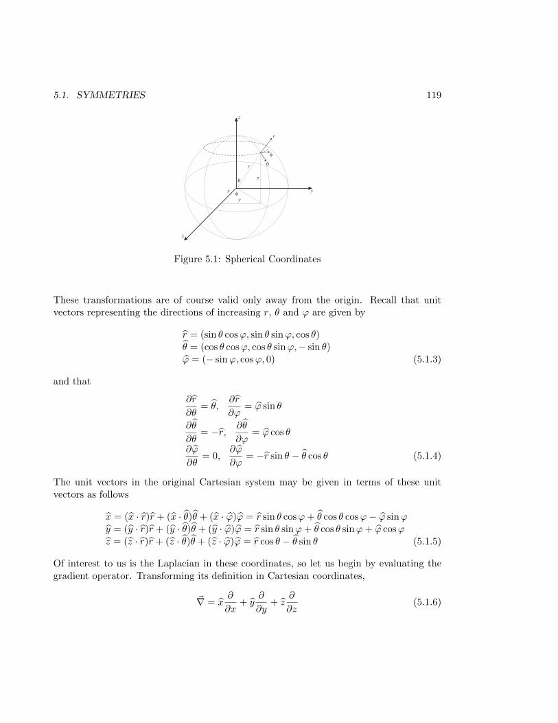
5.1. SYMMETRIES 119
r
q
f
y
y
z
z
xf
q
r
x
Figure 5.1: Spherical Coordinates
These transformations are of course valid only away from the origin. Recall that unitvectors representing the directions of increasing r, θ and ϕ are given by
r = (sin θ cosϕ, sin θ sinϕ, cos θ)θ = (cos θ cosϕ, cos θ sinϕ,− sin θ)ϕ = (− sinϕ, cosϕ, 0) (5.1.3)
and that
∂r
∂θ= θ,
∂r
∂ϕ= ϕ sin θ
∂θ
∂θ= −r, ∂θ
∂ϕ= ϕ cos θ
∂ϕ
∂θ= 0,
∂ϕ
∂ϕ= −r sin θ − θ cos θ (5.1.4)
The unit vectors in the original Cartesian system may be given in terms of these unitvectors as follows
x = (x · r)r + (x · θ)θ + (x · ϕ)ϕ = r sin θ cosϕ+ θ cos θ cosϕ− ϕ sinϕy = (y · r)r + (y · θ)θ + (y · ϕ)ϕ = r sin θ sinϕ+ θ cos θ sinϕ+ ϕ cosϕz = (z · r)r + (z · θ)θ + (z · ϕ)ϕ = r cos θ − θ sin θ (5.1.5)
Of interest to us is the Laplacian in these coordinates, so let us begin by evaluating thegradient operator. Transforming its definition in Cartesian coordinates,
~∇ = x∂
∂x+ y
∂
∂y+ z
∂
∂z(5.1.6)
120 CHAPTER 5. MOTION UNDER A CENTRAL FORCE
to spherical coordinates by using the transformations just given, we find1
~∇ = r∂
∂r+θ
r
∂
∂θ+
ϕ
r sin θ
∂
∂ϕ(5.1.7)
and taking the inner product2 we obtain the Laplacian in spherical coordinates
~∇2 =1
r2∂r(r
2∂r) +1
r2 sin θ∂θ(sin θ∂θ) +
1
r2 sin2 θ∂2ϕ (5.1.8)
The Euclidean distance between two points may be given in terms of r, θ and ϕ bytransforming its expression in Cartesian coordinates,
d~r2 = dx2 + dy2 + dz2 = dr2 + r2(dθ2 + sin2 θdϕ2) (5.1.9)
The volume element must account for the Jacobian of the transformation from the Carte-sian system to the spherical system,
J =∂(x, y, z)
∂(r, θ, ϕ)=
∂x∂r
∂x∂θ
∂x∂ϕ
∂y∂r
∂y∂θ
∂y∂ϕ
∂z∂r
∂z∂θ
∂z∂ϕ
(5.1.10)
i.e., ∫d3~r =
∫dxdydz =
∫drdθdϕdet(J) =
∫(r2 sin θ)drdθdφ (5.1.11)
gives the volume of spheres.
5.1.2 Cylindrical coordinates
Cylindrical coordinates are defined by the following transformations from a Cartesiansystem:
ρ =√x2 + y2
ϕ = tan−1(yx
)z = z (5.1.12)
where, we have assumed that the axial symmetry is about the “z” axis. The inversetransformations are simple to obtain
x = ρ cosϕ
1Problem: Show this.2Problem: Show this. Note that the gradient is a vector operator, so be careful to take appropriate
derivatives when necessary while taking the inner product.
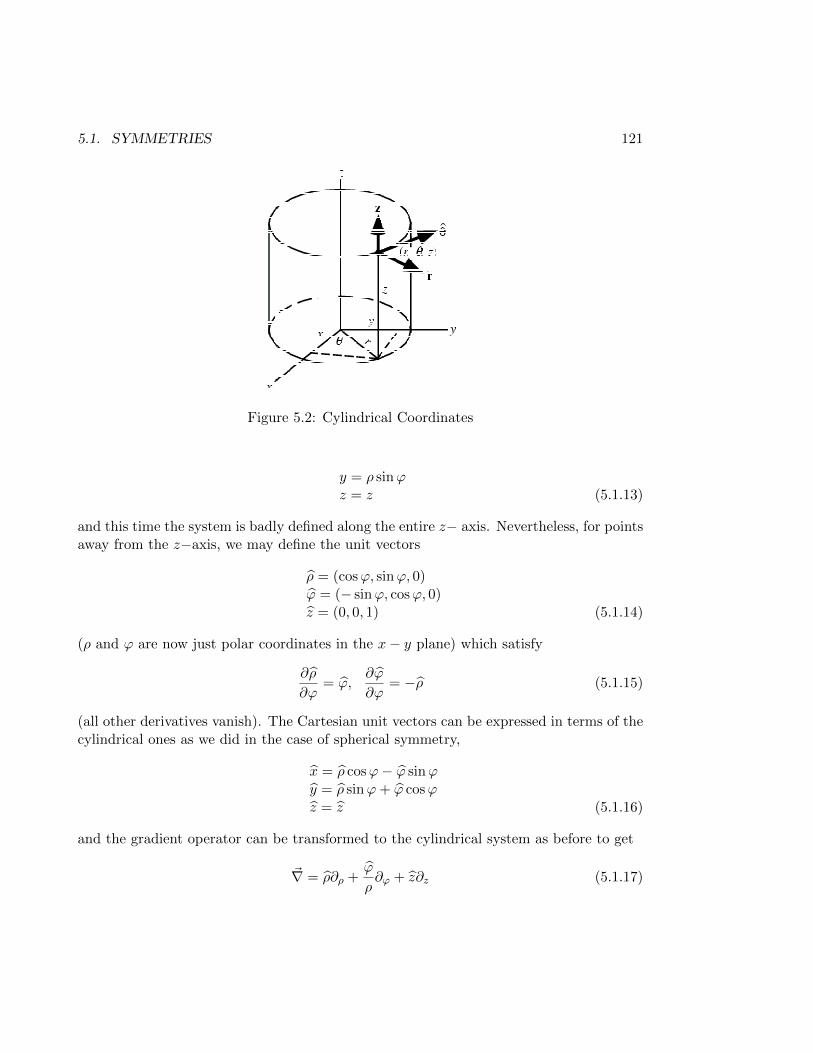
5.1. SYMMETRIES 121
Figure 5.2: Cylindrical Coordinates
y = ρ sinϕz = z (5.1.13)
and this time the system is badly defined along the entire z− axis. Nevertheless, for pointsaway from the z−axis, we may define the unit vectors
ρ = (cosϕ, sinϕ, 0)ϕ = (− sinϕ, cosϕ, 0)z = (0, 0, 1) (5.1.14)
(ρ and ϕ are now just polar coordinates in the x− y plane) which satisfy
∂ρ
∂ϕ= ϕ,
∂ϕ
∂ϕ= −ρ (5.1.15)
(all other derivatives vanish). The Cartesian unit vectors can be expressed in terms of thecylindrical ones as we did in the case of spherical symmetry,
x = ρ cosϕ− ϕ sinϕy = ρ sinϕ+ ϕ cosϕz = z (5.1.16)
and the gradient operator can be transformed to the cylindrical system as before to get
~∇ = ρ∂ρ +ϕ
ρ∂ϕ + z∂z (5.1.17)
122 CHAPTER 5. MOTION UNDER A CENTRAL FORCE
giving
~∇2 =1
ρ∂ρ(ρ∂ρ) +
1
ρ2∂2ϕ + ∂2
z (5.1.18)
The Euclidean distance between two points in these coordinates is
d~r2 = dρ2 + ρ2dϕ2 + dz2 (5.1.19)
Again, the volume element must account for the Jacobian of the transformation from theCartesian system to the spherical system,∫
d3~r =
∫dxdydz =
∫dρdϕdzdet(J) =
∫ρdρdϕdz (5.1.20)
gives the volume of cylinders.
5.2 Central Forces
A central force is any force of the form
~F (~r) = F (r)r (5.2.1)
where r is the unit outgoing radial vector from some fixed point, called the origin of theforce. The magnitude of the force depends only on the distance from the fixed point sothat it is the same at all points on the surface of a sphere with its center at the origin offorce. Central forces have the following two important properties:
1. Every central force is conservative. This can be seen by verifying that ~∇× ~F = 0,
~∇× ~F = (~∇F )× r + F (~∇× r) (5.2.2)
both terms of which vanish, the first because ~∇F (r) = F ′(r)r is in the radial directionand the second because r is irrotational. It follows there exists a (potential energy)function, φ = φ(r), such that F = −~∇φ(r).
2. Motion under a central force is torsion free. This is seen by evaluating rate of change
of ~F . Usingdr
dt= r · ~v, dr
dt=~v
r− r
r(r · ~v) (5.2.3)
we determine
~F (r) = F ′(r)(r · ~v)r +F (r)
r[~v − (r · ~v)r] (5.2.4)
and therefore
~F × ~F =F 2(r)
r(r × ~v) (5.2.5)
5.2. CENTRAL FORCES 123
showing that ~v ·(~F × ~F ) = 0. This leads to the important conclusion that the motionwill always occur in the plane determined by the initial velocity and the force itself.
Another way to arrive at the last conclusion is to consider Newton’s equations in sphericalcoordinates. Taking a time derivative of the position vector
~r = rr (5.2.6)
and using (5.1.4), gives
d~r
dt=dr
dtr + r
dr
dt= rr + rθθ + r sin θϕϕ. (5.2.7)
Taking a derivative once more,
d2~r
dt2= (r − rθ2 − rϕ2 sin2 θ)r + (2rθ + rθ − rϕ2 sin θ cos θ)θ
+(2rϕ sin θ + 2rϕθ cos θ + rϕ sin θ)ϕ. (5.2.8)
Now according to Newton’s second law
md2~r
dt2= F (r)r (5.2.9)
assuming that the force is central. If we orient our coordinate system in such a way thatthe initial velocity is in the x − y plane (θ = π
2 ) i.e., θ(t = 0) = 0, we find (from the θcomponent)
θ(t = 0) = 0 (5.2.10)
i.e., the motion will stay forever in the x − y plane. This greatly simplifies the problembecause it means that motion under a central force is effectively two dimensional. Therelevant two components of the equation of motion give
m(r − rϕ2) = F (r)
2rϕ+ rϕ = 0 (5.2.11)
Of course, if the initial velocity of the particle is such that ϕ(t = 0) = 0 then the secondequation gives ϕ(t = 0) = 0, which means that the motion is forever radial or one dimen-sional, but this is not the most general situation because it involves a restriction on theinitial velocity. On the other hand, because it is always possible to orient the x− y planeso that it coincides with the plane defined by the radial vector and the (arbitrary) initialvelocity the motion will always be at most two dimensional.
124 CHAPTER 5. MOTION UNDER A CENTRAL FORCE
The second of (5.2.11) can be integrated quite easily and we find
2r
r= − ϕ
ϕ⇒ ln r2 = ln
L
mϕ, (5.2.12)
where we have written the integration constant in the form L/m. A more convenient wayto express the solution is
mr2ϕ = L, (5.2.13)
which should make it apparent that L is, in fact, the angular momentum of the body.Solving for ϕ and inserting the solution into the first equation in (5.2.11) gives
mr − L2
mr3= F (5.2.14)
which is an equation for r = r(t). The second term on the right, −L2/mr3, is the masstimes the centripetal acceleration required to keep the body moving around the center ofthe force. The equation can be integrated once,
mr = mrdr
dr= F +
L2
mr3⇒ 1
2mr2 +
L2
2mr2−∫Fdr = E (5.2.15)
where E is also an integration constant, which will be recognized as the total energy of thebody . The first term on the left is the radial kinetic energy. The second is the rotationalkinetic energy and the last term is the potential energy associated with the central force,
φ(r) = −∫ r
F (r′)dr′. (5.2.16)
Thus the quantity
V (r) = φ(r) +L2
2mr2(5.2.17)
has the form of an effective potential energy in (5.2.15). To understand its origin, turnagain to the equation of motion (5.2.14) and write it as
mr = F (r) +L2
mr3(5.2.18)
The extra “force” on the right hand side is directed outward and corresponds to thefictitious centrifugal force that an observer on the rotating body would feel. It correspondsto a potential
φ′(r) = −∫ r
dr′L2
mr′3=
L2
2mr2(5.2.19)
5.3. INVERSE SQUARE FORCE 125
showing that V (r) is the effective potential energy measured by the observer who is at-tached to the orbiting body. The energy equation,
r =
√2
m[E − V (r)], (5.2.20)
can be formally integrated, to give∫ r
r0
dr′√E − V (r′)
=
√2
m(t− t0) (5.2.21)
Of course, the problem is to perform the integral on the left. If this is done, we obtain theradius of the body from the force center as a function of time, r = r(t), and then ϕ = ϕ(t)directly from the first equation in (5.2.11). Thus,
ϕ =dϕ
dt=
L
mr2⇒ ϕ− ϕ0 =
L
m
∫ t
t0
dt′
r2(t′)(5.2.22)
In principle, this solves the central force problem.Parametric solutions, with time as the parameter, are difficult to visualize. If possible,
in two dimensions it’s desirable to obtain the solution in function form. In this particularcase, it means that we should seek a solution of the form r = r(θ). rewrite (5.2.20) as
r =dr
dϕϕ =
L
mr2
dr
dϕ=
√2
m[E − V (r)] (5.2.23)
or ∫ r
r0
dr/r2√E − V (r)
=
√2m
L2(ϕ− ϕ0) (5.2.24)
where (r0, ϕ0) are the polar coordinates of the object at the initial time. If we could solvethe integral on the left we would get a relationship between r and ϕ, which would have tobe inverted to obtain r = r(ϕ).
5.3 Inverse square force
For an inverse square central force,
F (r) =k
r2, (5.3.1)
where k is positive for a repulsive force and negative for an attractive force (such as gravity)the potential energy is
φ(r) = −∫ r
dr′F (r′) =k
r(5.3.2)
126 CHAPTER 5. MOTION UNDER A CENTRAL FORCE
and the integral equation becomes∫ r
r0
dr/r2√E − k
r −L2
2mr2
=
√2m
L2(ϕ− ϕ0) (5.3.3)
Now if we substitute u = 1/r, we have
−∫ u
u0
du√E − ku− L2u2
2m
=
√2m
L2(ϕ− ϕ0) (5.3.4)
The integral on the left is easily solved by completion of squares and further substitutions.Completing squares first, express the equation as
−∫ u
u0
du√(E + mk2
2L2
)−(
Lu√2m
+√
m2kL
)2=
√2m
L2(ϕ− ϕ0) (5.3.5)
Evidently, for real solutions, we require
E = E +mk2
2L2> 0 (5.3.6)
so let
w =Lu√2m
+
√m
2
k
L, dw =
Ldu√2m
(5.3.7)
Then
−∫ w
w0
dw′√E − w′2
= (ϕ− ϕ0) (5.3.8)
and the integral on the left (substitute w = E cos η) is solved to give
cos−1 w
E− cos−1 w0
E= (ϕ− ϕ0) (5.3.9)
or
w =Lu√2m
+
√m
2
k
L=√E cos(ϕ− ϕ0) (5.3.10)
where ϕ0 has been redefined to accommodate the constant term arising in the integral onthe left. Solving for u we find
u =1
r=m|k|L2
[−sgn(k) +
√1 +
2EL2
mk2cos(ϕ− ϕ0)
](5.3.11)
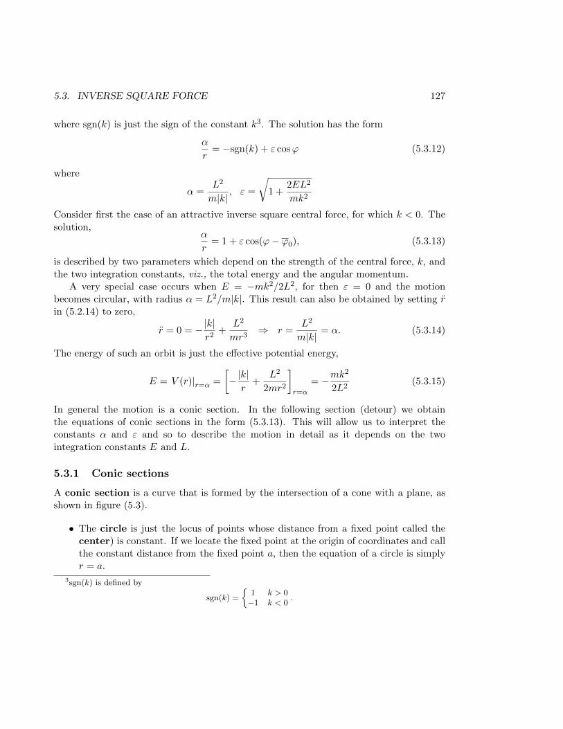
5.3. INVERSE SQUARE FORCE 127
where sgn(k) is just the sign of the constant k3. The solution has the form
α
r= −sgn(k) + ε cosϕ (5.3.12)
where
α =L2
m|k|, ε =
√1 +
2EL2
mk2
Consider first the case of an attractive inverse square central force, for which k < 0. Thesolution,
α
r= 1 + ε cos(ϕ− ϕ0), (5.3.13)
is described by two parameters which depend on the strength of the central force, k, andthe two integration constants, viz., the total energy and the angular momentum.
A very special case occurs when E = −mk2/2L2, for then ε = 0 and the motionbecomes circular, with radius α = L2/m|k|. This result can also be obtained by setting rin (5.2.14) to zero,
r = 0 = −|k|r2
+L2
mr3⇒ r =
L2
m|k|= α. (5.3.14)
The energy of such an orbit is just the effective potential energy,
E = V (r)|r=α =
[−|k|r
+L2
2mr2
]r=α
= −mk2
2L2(5.3.15)
In general the motion is a conic section. In the following section (detour) we obtainthe equations of conic sections in the form (5.3.13). This will allow us to interpret theconstants α and ε and so to describe the motion in detail as it depends on the twointegration constants E and L.
5.3.1 Conic sections
A conic section is a curve that is formed by the intersection of a cone with a plane, asshown in figure (5.3).
• The circle is just the locus of points whose distance from a fixed point called thecenter) is constant. If we locate the fixed point at the origin of coordinates and callthe constant distance from the fixed point a, then the equation of a circle is simplyr = a.
3sgn(k) is defined by
sgn(k) =
1 k > 0−1 k < 0
.
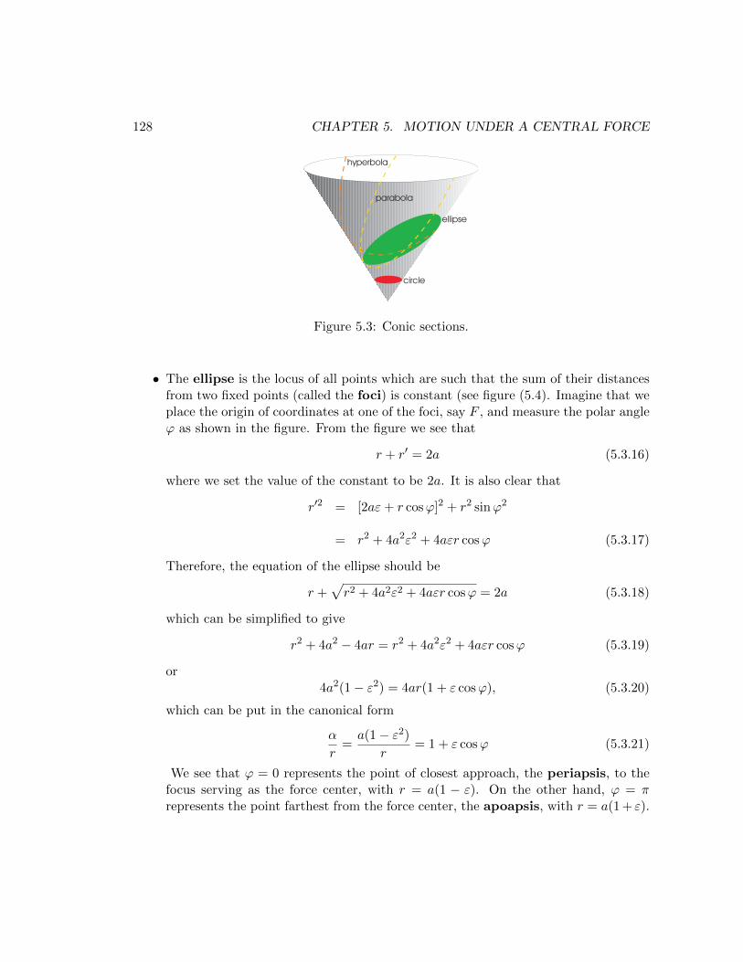
128 CHAPTER 5. MOTION UNDER A CENTRAL FORCE
Figure 5.3: Conic sections.
• The ellipse is the locus of all points which are such that the sum of their distancesfrom two fixed points (called the foci) is constant (see figure (5.4). Imagine that weplace the origin of coordinates at one of the foci, say F , and measure the polar angleϕ as shown in the figure. From the figure we see that
r + r′ = 2a (5.3.16)
where we set the value of the constant to be 2a. It is also clear that
r′2 = [2aε+ r cosϕ]2 + r2 sinϕ2
= r2 + 4a2ε2 + 4aεr cosϕ (5.3.17)
Therefore, the equation of the ellipse should be
r +√r2 + 4a2ε2 + 4aεr cosϕ = 2a (5.3.18)
which can be simplified to give
r2 + 4a2 − 4ar = r2 + 4a2ε2 + 4aεr cosϕ (5.3.19)
or4a2(1− ε2) = 4ar(1 + ε cosϕ), (5.3.20)
which can be put in the canonical form
α
r=a(1− ε2)
r= 1 + ε cosϕ (5.3.21)
We see that ϕ = 0 represents the point of closest approach, the periapsis, to thefocus serving as the force center, with r = a(1 − ε). On the other hand, ϕ = πrepresents the point farthest from the force center, the apoapsis, with r = a(1 + ε).
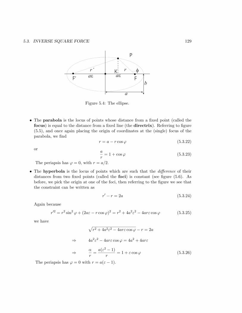
5.3. INVERSE SQUARE FORCE 129
Figure 5.4: The ellipse.
• The parabola is the locus of points whose distance from a fixed point (called thefocus) is equal to the distance from a fixed line (the directrix). Referring to figure(5.5), and once again placing the origin of coordinates at the (single) focus of theparabola, we find
r = a− r cosϕ (5.3.22)
ora
r= 1 + cosϕ (5.3.23)
The periapsis has ϕ = 0, with r = a/2.
• The hyperbola is the locus of points which are such that the difference of theirdistances from two fixed points (called the foci) is constant (see figure (5.6). Asbefore, we pick the origin at one of the foci, then referring to the figure we see thatthe constraint can be written as
r′ − r = 2a (5.3.24)
Again because
r′2 = r2 sin2 ϕ+ (2aε− r cosϕ)2 = r2 + 4a2ε2 − 4arε cosϕ (5.3.25)
we have √r2 + 4a2ε2 − 4arε cosϕ− r = 2a
⇒ 4a2ε2 − 4arε cosϕ = 4a2 + 4arε
⇒ α
r=a(ε2 − 1)
r= 1 + ε cosϕ (5.3.26)
The periapsis has ϕ = 0 with r = a(ε− 1).
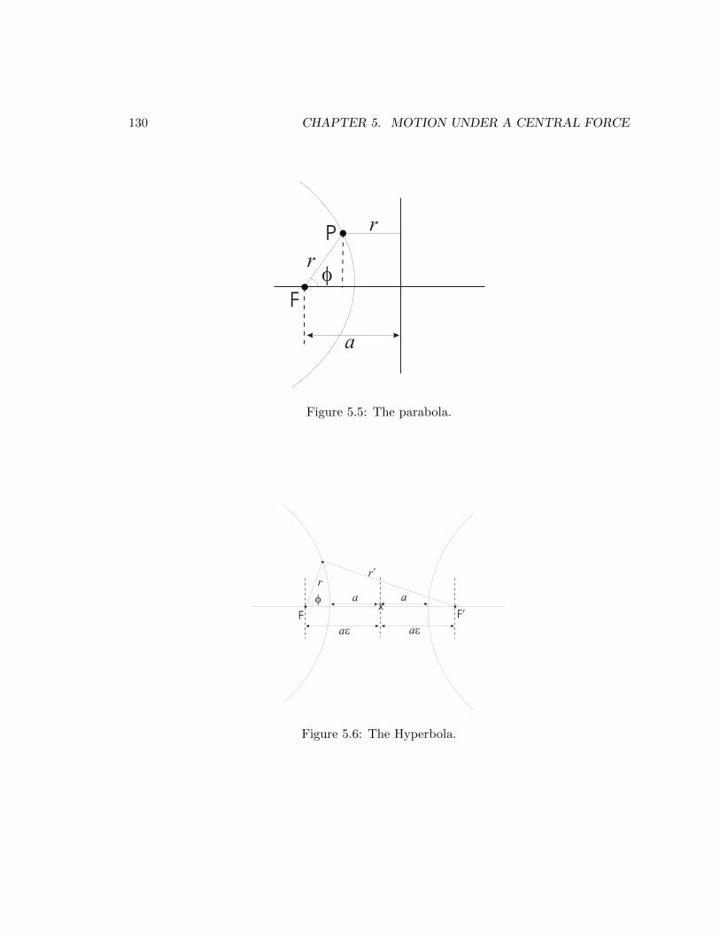
130 CHAPTER 5. MOTION UNDER A CENTRAL FORCE
Figure 5.5: The parabola.
Figure 5.6: The Hyperbola.
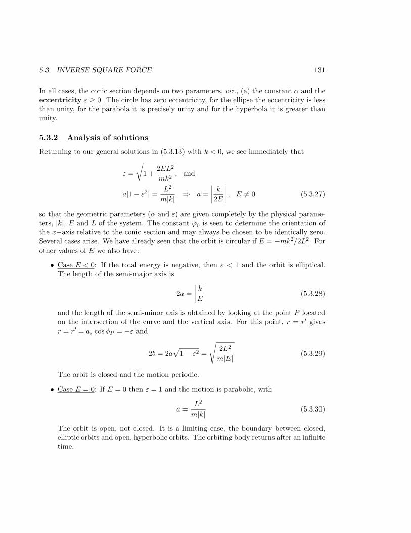
5.3. INVERSE SQUARE FORCE 131
In all cases, the conic section depends on two parameters, viz., (a) the constant α and theeccentricity ε ≥ 0. The circle has zero eccentricity, for the ellipse the eccentricity is lessthan unity, for the parabola it is precisely unity and for the hyperbola it is greater thanunity.
5.3.2 Analysis of solutions
Returning to our general solutions in (5.3.13) with k < 0, we see immediately that
ε =
√1 +
2EL2
mk2, and
a|1− ε2| = L2
m|k|⇒ a =
∣∣∣∣ k2E∣∣∣∣ , E 6= 0 (5.3.27)
so that the geometric parameters (α and ε) are given completely by the physical parame-ters, |k|, E and L of the system. The constant ϕ0 is seen to determine the orientation ofthe x−axis relative to the conic section and may always be chosen to be identically zero.Several cases arise. We have already seen that the orbit is circular if E = −mk2/2L2. Forother values of E we also have:
• Case E < 0: If the total energy is negative, then ε < 1 and the orbit is elliptical.The length of the semi-major axis is
2a =
∣∣∣∣ kE∣∣∣∣ (5.3.28)
and the length of the semi-minor axis is obtained by looking at the point P locatedon the intersection of the curve and the vertical axis. For this point, r = r′ givesr = r′ = a, cosφP = −ε and
2b = 2a√
1− ε2 =
√2L2
m|E|(5.3.29)
The orbit is closed and the motion periodic.
• Case E = 0: If E = 0 then ε = 1 and the motion is parabolic, with
a =L2
m|k|(5.3.30)
The orbit is open, not closed. It is a limiting case, the boundary between closed,elliptic orbits and open, hyperbolic orbits. The orbiting body returns after an infinitetime.
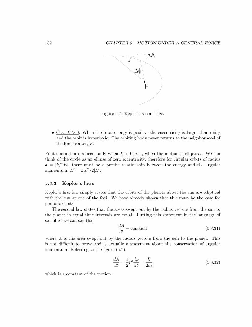
132 CHAPTER 5. MOTION UNDER A CENTRAL FORCE
Figure 5.7: Kepler’s second law.
• Case E > 0: When the total energy is positive the eccentricity is larger than unityand the orbit is hyperbolic. The orbiting body never returns to the neighborhood ofthe force center, F .
Finite period orbits occur only when E < 0, i.e., when the motion is elliptical. We canthink of the circle as an ellipse of zero eccentricity, therefore for circular orbits of radiusa = |k/2E|, there must be a precise relationship between the energy and the angularmomentum, L2 = mk2/2|E|.
5.3.3 Kepler’s laws
Kepler’s first law simply states that the orbits of the planets about the sun are ellipticalwith the sun at one of the foci. We have already shown that this must be the case forperiodic orbits.
The second law states that the areas swept out by the radius vectors from the sun tothe planet in equal time intervals are equal. Putting this statement in the language ofcalculus, we can say that
dA
dt= constant (5.3.31)
where A is the area swept out by the radius vectors from the sun to the planet. Thisis not difficult to prove and is actually a statement about the conservation of angularmomentum! Referring to the figure (5.7),
dA
dt=
1
2r2dϕ
dt=
L
2m(5.3.32)
which is a constant of the motion.

5.3. INVERSE SQUARE FORCE 133
Kepler’s third law gives the relationship between the period of the orbit and the lengthof the semi-major axis. It states that the square of the period is proportional to the cubeof the semi-major axis, i.e., τ2 ∝ a3, where τ is the period, or the time taken to completeone orbit. Proving this takes a bit of work, but this is the law that motivated Newton todescribe gravity by an inverse square central force. Begin by noting that integrating thesecond law over an entire period gives the area of the ellipse
A =Lτ
2m(5.3.33)
However, the area of the ellipse is obtained by integrating the expression
dA =1
2r2dϕ (5.3.34)
over the entire ellipse. Using the solutions obtained,
A =α2
2
∫ 2π
0
dϕ
(1 + ε cosϕ)2= πa2
√1− ε2 (5.3.35)
Therefore,
Lτ
2m= πa2
√1− ε2 ⇒ τ = π
√mk2
2|E|3, (5.3.36)
the right hand side of which can be expressed in terms of the length of the semi-majoraxis, using (5.3.27),
τ2 =4π2m
ka3 (5.3.37)
For the gravitational force, the constant k is proportional to the mass of the body, which isjust a statement of the weak equivalence principle. The proportionality constant betweenthe square of the radius and the cube of the semi-major axis is therefore independent ofthe mass of the orbiting body. For instance, for a star-planet system, assuming that themass of the star, M, is very much larger than the mass of the planet so that it is for allpractical purposes fixed,
k = GMm ⇒ τ2 =4π2
GMa3 (5.3.38)
When the mass of the planet is not negligible compared to the mass of the star, we maystill use the description of the motion as given above, provided we interpret the resultsconsistently. In that case, the coordinate r should be understood as the magnitude of therelative coordinate, ~r = ~rp − ~r, the mass of the orbiting body, m, should be replacedby the reduced mass, µ, of the system and the mass of the star by the total mass. The
134 CHAPTER 5. MOTION UNDER A CENTRAL FORCE
force center is then the center of mass of the system. Because no external forces act on anisolated system, the center of mass moves as though it were a free particle. In other words,the star-planet system may move as a whole freely through space while each member ofthe system orbits about the center of mass.
5.4 Other examples of central forces
The inverse square force is by no means the only physically important example of a centralforce. The force exerted by a spring that is fixed at one end, for example, is a central forcefor which F (r) = −k(r− r0), where r0 is the equilibrium length of the spring and k is thespring constant. The negative sign indicates that the force is attractive so long as r > r0
(the spring is stretched) and repulsive when r < r0. The corresponding potential energyis evidently
φ(r) = −∫ r
r0
F (r)dr =1
2k(r − r0)2. (5.4.1)
Another important example of a central force is the Yukawa force,
F (r) =k
r2e−r/r0
[1 +
r
r0
], (5.4.2)
which is often used to describe the effective weak interactions between mesons. It isapproximately inverse square so long as r/r0 1, but decreases rapidly at large distances,i.e., when r/r0 1. It is deemed a “short-range” force, as opposed to the inverse-squareforce, which is considered “long range”. The potential energy corresponding to this forceis the Yukawa potential,
φ(r) = −∫ r
∞F (r)dr =
k
re−r/r0 . (5.4.3)
There are also generalizations of the inverse square force, with F (r) = k/rn, where n is apositive integer. The potential energy is
φ(r) = −∫ r
∞F (r)dr =
k
(n− 1)rn−1(5.4.4)
For n > 2, such terms arise, for example, as general relativistic corrections to Newton’sinverse square law of gravity, but they are not so interesting on their own.
For each of the forces above, our starting point will be (5.2.24). As an example,consider Hooke’s Law. For simplicity, take r0 = 0, then the effective potential in this caseis
V (r) =L2
2mr2+
1
2kr2 (5.4.5)
5.4. OTHER EXAMPLES OF CENTRAL FORCES 135
and (5.2.24) determines the two dimensional motion according to∫ r
r0
dr/r2√E − L2
2mr2− 1
2kr2
=
√2m
L2(ϕ− ϕ0). (5.4.6)
The problem is to evaluate the integral on the left. It is convenient to make the substitutionu = 1/r2, which gives
− 1
2
∫ r
u0
du√Eu− L2u2
2m −k2
=
√2m
L2(ϕ− ϕ0) (5.4.7)
or, completing squares,
− 1
2
∫ u
u0
du√(mE
2
2L2 − k2 )− (
√m2EL −
Lu√2m
)2=
√2m
L2(ϕ− ϕ0) (5.4.8)
Evidently, for real solutions,
E =mE2
2L2− k
2> 0 (5.4.9)
and substituting w =√
m2EL −
Lu√2m
gives
1
2
∫ w
w0
dw√E − w2
= (ϕ− ϕ0)⇒ w = −√E cos 2(ϕ− ϕ0) (5.4.10)
where we have redefined ϕ0 to accommodate the additional constant obtained by integrat-ing the left hand side. In terms of r, we find a solution of the form
α2
r2= 1 + ε cos 2(ϕ− ϕ0) (5.4.11)
where
α =L√mE
, ε =
√1− kL2
mE2(5.4.12)
and circular orbits are possible if E = (kL2/m)1/2 (i.e., when ε = 0), in which case theradius of a circular orbit is r = (L2/mk)1/4. This is the minimum permissible energy fortwo dimensional motion.4
The solution in (5.4.11) describes an ellipse provided that ε < 1. This can be madeexplicit by making the transformations x = r cosϕ, y = r sinϕ and taking ϕ0 = 0 for
4Problem: Determine the energy and radius of a circular orbit in terms of the angular momentum usingthe condition r = 0 in (5.2.14).
136 CHAPTER 5. MOTION UNDER A CENTRAL FORCE
convenience (this amounts only to choosing an orientation of the axes for the Cartesiansystem so that the periapsis occurs at ϕ = 0). We find
α2
r2= 1 + ε cos 2ϕ ⇒ x2
α2/(1 + ε)+
y2
α2/(1− ε)= 1, (5.4.13)
showing that the center of the force is at the center of the ellipse.5
Kepler’s second law is true for elliptical orbits caused by any central force because itis just a restatement of the law of conservation of momentum. The period, however, doesdepend on the particular form of the force. In this case, it turns out to be independent ofthe length of the major axis. We find,
A =Lτ
2m=α2
2
∫ 2π
0
dϕ
(1 + ε cos 2ϕ)=
πα2
√1− ε2
=πL√km
(5.4.14)
gives
τ = 2π
√m
k, (5.4.15)
which is precisely the period of one dimensional oscillations.
5.5 Stability of Circular Orbits
We have seen that the equations describing the motion of an object under the action of acentral force are
m(r − rϕ2) = F (r)
2rϕ+ rϕ = 0 (5.5.1)
We also discovered that the second is integrable, giving a conshtant of the motion, theangular momentum, and that it can be combined with the first to give one equation forthe radial motion
mr = F (r) +L2
mr3(5.5.2)
5Problem: By transforming to Cartesian coordinates, show that the orbit given by
a(1− ε2)
r= 1 + ε cosϕ
(ε < 1) is an ellipse, but that the force center is located at one focus of the ellipse in this case. Show alsothat the distance from the center of the ellipse to the focus is aε. Hint: Choose a convenient orientationof the Cartesian axes by selecting ϕ0, then show that the equation, written in Cartesian coordinates, isthe equation of an ellipse, horizontally shifted a distance −aε.
5.5. STABILITY OF CIRCULAR ORBITS 137
Now it is quite clear that, no matter what the form of F (r), there will always be circularorbits so long as ~F is attractive: simply solve
F (r) = − L2
mr3(5.5.3)
to get the radius of the circle. This is of course just the condition that the effectivepotential has an extremum at r0 because
V ′(r0) = φ′(r0)− L2
mr30
= 0⇒ F (r0) = − L2
mr3. (5.5.4)
Let us examine the stability of these circular orbits, first in general and then for someparticular cases. An orbit will be considered stable if it does not run away, or changedrastically when it is perturbed by some external influence. We will make this intuitiveidea more precise below.
Suppose that the solution to (5.5.3) is r0, then imagine that we perturb the orbitslightly so that r = r0 + x, where x/r0 1. Evidently, r = x and the equation of motionbecomes
mx = F (r0 + x) +L2
m(r0 + x)3(5.5.5)
Since x r0, we expand in a Taylor series about x = 0, retaining only the first orderterm in x/r0. Then
mx = F (r0) +L2
mr30
+ F ′(r0)x− 3L2x
mr40
+ . . . (5.5.6)
The first two terms on the right vanish because r0 is the radius of the circular orbit [see(5.5.3)]. Then the equation for the perturbation, x, becomes
mx = −(
3L2
mr40
− F ′(r0)
)x = −κx (5.5.7)
and may be compared to the equation of a one dimensional harmonic oscillator, with forceconstant κ. We understand these solutions quite well. If the force constant is positivethere are oscillations about x = 0, but if the force constant is negative then x may growexponentially, without bound. The perturbations continue small when the κ is positiveand that is therefore our condition for stability. It cannot have escaped you that we canthink of this condition as the requirement that the effective potential has a well definedminimum at r = r0 (not simply an extremum) because
V ′′(r0) = −F ′(r0) +3L2
mr40
(5.5.8)
138 CHAPTER 5. MOTION UNDER A CENTRAL FORCE
which we have just seen must be larger than zero for stability.
As an example, if
F (r) = − k
rn(5.5.9)
the radius of the circular orbits would be given by
k
rn0=
L2
mr30
⇒ rn−30 =
mk
L2(5.5.10)
and in particular when n = 2 we have
r0 =L2
mk(5.5.11)
Are these circular orbits stable? Let us examine the condition for stability:
3L2
mr40
− nk
rn+10
> 0⇒ rn−30 >
nmk
3L2(5.5.12)
or simply (inserting the value of r0 found above) n < 3. In this case, any perturbationcauses the body to oscillate about the stable circular orbit with an angular frequency of
ω =L
mr20
√3− n (5.5.13)
The solution for x, up to this order of approximation is then
x = A1 cosωt = A1 cos(√
3− nϕ)
(5.5.14)
where we used (5.2.13) and r = r0. Clearly, for closed orbits we must ask for
√3− n =
p
q= β (5.5.15)
where p/q is a rational number. It this way the perturbation x would return to itself afterq rotations through an angle of 2π. Therefore, for rational β and
F (r) = − k
r3−β2 (5.5.16)
the circular orbits are not only stable against small perturbations, but they are also closed.
5.5. STABILITY OF CIRCULAR ORBITS 139
5.5.1 Bertand’s Theorem
If we seek more stringent conditions on the force law, so orbits remain closed even when thedeviations from circularity are large (i.e., if we wish to beyond the linear approximation)then the analysis is more complicated. It is convenient to rewrite the radial equation ofmotion in (5.2.11) in terms of u(ϕ) = 1/r(ϕ) as
d2u
dϕ2+ u = −m
L2
dφ(u)
du
def= Q(u) (5.5.17)
Perfectly circular orbits are recovered when u′(ϕ) = 0, or u0 = Q(u0). First consider smalldeviations from circularity, u = u0 + u(ϕ); in the linear approximation,
d2y
dϕ2+ u0 + y = Q(u0) + yQ′(u0) (5.5.18)
ord2y
dϕ2+ [1−Q′(u0)]y = 0 (5.5.19)
whose solution is clearly y = A cos(βϕ), where A is an integration constant and β2 =1−Q′(u0) must be greater than zero for a stable orbit and rational for closed orbits. Thisis just the result we had before.6
To go beyond the linear approximation, we retain higher order terms in the seriesexpansion of Q(u),
d2y
dϕ2+ β2y =
1
2!Q′′(u0)y2 +
1
3!Q′′′(u0)y3 + . . . (5.5.20)
Now the behavior of y(ϕ) to linear order is the first term of a Fourier expansion in βϕ.We therefore seek a closed orbit solution by including more terms of the Fourier series,taking
y(ϕ) = A0 +A1 cosβϕ+A2 cos 2βϕ+A3 cos 3βϕ+ . . . (5.5.21)
The coefficients A0 and A2 are of higher order (smaller) than A1, as can be seen in theapproach to circularity. Moreover, A3 will be smaller than A0 and A2, A4 will be smallerthan A3 and so on (we will see this shortly). Therefore, in the expansion (5.5.20), if weinclude terms up to cos(3βϕ) in y (third order), then we include only terms up to cos(2βϕ)in y2 and cos(βϕ) in y3. Make use of the fact that the set
1√2,
cos(nβϕ)∣∣ n ∈ Z+
6Taking F (r) = k/rn, determine (a) Q(u), (b) the radius of circular orbits and (c) β. Confirm the
earlier results.
140 CHAPTER 5. MOTION UNDER A CENTRAL FORCE
is an orthonormal and complete basis for even, periodic functions, with inner product
〈cos(nβϕ), cos(mβϕ)〉 def=
β
π
∫ 2π/β
0dϕ [cos(nβϕ), cos(mβϕ)] = δmn, (5.5.22)
to reduce higher powers of cos(nβφ) and products as, for example,
cos2(βϕ) =1
2〈cos2 βϕ, 1〉+
∑n
〈cos2 βϕ cos(nβϕ)〉 cos(nβϕ) =1
2(1 + cos(2βϕ))
cos3(βϕ) =1
4(3 cos(βϕ) + cos(3βϕ))
cos(βϕ) cos(2βϕ) =1
2(cos(βϕ) + cos(3βϕ)) (5.5.23)
and so on. Carefully expanding (5.5.20), we find
A0 =A2
1
4β2Q′′(u0)
A2 = − A1
12β2Q′′(u0)
A3 = − 1
16β3
[A1A2Q
′′(u0) +A3
1
12Q′′′(u0)
](5.5.24)
as well as one constraint,
−A0A1Q′′(u0)− 1
2A1A2Q
′′(u0)− 1
8A3
1Q′′′(u0) = 0. (5.5.25)
We have already seen that F (r) = −k/r3−β2is necessary for stable orbits. This means
that
Q(u) =mk
L2u1−β2
(5.5.26)
and therefore the inverse radius of circular orbits is given by uβ2
0 = mk/L2. Then
Q′′(u0) = −β2(1− β2)
u0
Q′′′(u0) =β2(1− β4)
u20
, (5.5.27)
and inserting (5.5.24) and (5.5.27) into (5.5.25) shows that β must satisfy the (muchstronger) condition
β2(1− β2)(4− β2) = 0 (5.5.28)
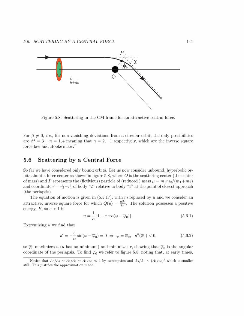
5.6. SCATTERING BY A CENTRAL FORCE 141
b+db
b
P
f0
c
O
Figure 5.8: Scattering in the CM frame for an attractive central force.
For β 6= 0, i.e., for non-vanishing deviations from a circular orbit, the only possibilitiesare β2 = 3 − n = 1, 4 meaning that n = 2,−1 respectively, which are the inverse squareforce law and Hooke’s law.7
5.6 Scattering by a Central Force
So far we have considered only bound orbits. Let us now consider unbound, hyperbolic or-bits about a force center as shown in figure 5.8, where O is the scattering center (the centerof mass) and P represents the (fictitious) particle of (reduced ) mass µ = m1m2/(m1 +m2)and coordinate ~r = ~r2−~r1 of body “2” relative to body “1” at the point of closest approach(the periapsis).
The equation of motion is given in (5.5.17), with m replaced by µ and we consider an
attractive, inverse square force for which Q(u) = µ|k|L2 . The solution possesses a positive
energy, E, so ε > 1 in
u =1
α[1 + ε cos(ϕ− ϕ0)] . (5.6.1)
Extremizing u we find that
u′ = − εα
sin(ϕ− ϕ0) = 0 ⇒ ϕ = ϕ0, u′′(ϕ0) < 0, (5.6.2)
so ϕ0 maximizes u (u has no minimum) and minimizes r, showing that ϕ0 is the angularcoordinate of the periapsis. To find ϕ0 we refer to figure 5.8, noting that, at early times,
7Notice that A0/A1 ∼ A2/A1 ∼ A1/u0 1 by assumption and A3/A1 ∼ (A1/u0)2 which is smallerstill. This justifies the approximation made.
142 CHAPTER 5. MOTION UNDER A CENTRAL FORCE
u(π) = 0 implies that ϕ0 = cos−1(1/ε). Thus the radial distance of the periapsis from thescattering center will be rP = α/(1 + ε) = a(ε− 1). The total deflection angle is given bythe condition that u = 0 and ϕ 6= π, i.e., referring to figure 5.8,
ϕ± − ϕ0 = ± cos−1
(−1
ε
)⇒ ϕ± = cos−1
(1
ε
)± cos−1
(−1
ε
). (5.6.3)
The solution with the positive sign yields π, which represents the situation at early times,so we pick the second solution
χ = ϕ− = cos−1
(1
ε
)− cos−1
(−1
ε
)= −2 sin−1
(1
ε
), (5.6.4)
as representative of the situation at late times. χ is the scattering angle. It dependsexclusively on the eccentricity.8 Larger eccentricities are scattered through smaller angles,but because the eccentricity depends on the energy and the angular momentum,
ε =
√1 +
2EL2
µk2, (5.6.5)
the higher the total energy and total angular momentum, the smaller will be the deflectionangle.
5.6.1 Differential Cross-Section
A problem of physical interest concerns the deflection of a beam of particles by a scatteringcenter, as in the case, for example, of Rutherford scattering. Typically, one is interestedin the differential scattering cross-section, which is the ratio of the number of particlesscattered in a solid angle between Ω and Ω + dΩ per unit time by the total number ofincident particles per unit area per unit time (flux),
dσ =# of particles scattered in dΩ
incident flux(5.6.6)
The mechanical dimension of the differential cross section is area. It may be thoughtof as the area, transverse to the relative velocity, within which the interacting objectsmust meet in order to scatter through a given solid angle. The differential solid angle isdΩ = 2π sinχdχ. If v∞ is the initial relative speed far from the scattering center, so thatthe initial relative velocity is ~v = v∞x in figure 5.8, we express the angular momentumand the total energy as
L = mv∞b, E =1
2µv2∞. (5.6.7)
8Problem: Perform a similar analysis for a repulsive central force, Q = −µ|k|L2 . Show that χ =
+2 sin−1(1/ε).
5.6. SCATTERING BY A CENTRAL FORCE 143
For particles of the same incident energy, the scattering angle χ depends only on theangular momentum and therefore only on b, then the number particles scattered betweenχ and dχ will pass through a ring of radius between b and b+db (again, refer to the figure),so dσ = 2πbdb, i.e.,
dσ
dΩ=
b
| sinχ|
∣∣∣∣ dbdχ∣∣∣∣ (5.6.8)
and the total cross-section is defined as
σT =
∫Ωdσ = 2π
∫ π
0dχ b
∣∣∣∣ dbdχ∣∣∣∣ . (5.6.9)
From σT , we may also define a total cross sectional radius, a, by equating σT to the area
of a disk of radius a, i.e., σTdef= πa2.
For the attractive, inverse square force we have examined above, because ε = −1/ sin(χ/2)it follows that
dε2
dχ=
2µ2v4∞bdb/dχ
k2= − cosχ/2
sin3 χ/2(5.6.10)
and thereforedσ
dΩ=
b
| sinχ|
∣∣∣∣ dbdχ∣∣∣∣ =
(k csc2 χ/2
4E
)2
(5.6.11)
The total differential cross section is infinite! This is because the force we have consideredis long range. In the Rutherford experiment, it is screened by the electrons in the atom.
5.6.2 Dynamical “Friction” (Chandrashekar)*
As our treatment above has dealt exclusively with the relative coordinate, we have hadlittle explicit information regarding the motion of the masses themselves. Let us close thischapter by addressing the motion of the individual masses. Conservation of momentumrequires that
m1d~v1
dt+m2
d~v2
dt= 0 (5.6.12)
so if we set ~v = ~v2 − ~v1, then it follows that the rate of change of each velocity dependsonly on the rate of change of ~v,
d~v1
dt= −m2
M
d~v
dt,d~v2
dt=m1
M
d~v
dt(5.6.13)
As before, we denote by b the impact parameter and ~v− = v∞x the velocity as t → −∞,so L = µbv∞ and E = 1
2µv2∞ and both, being conserved, have the same values as t→ +∞.
Thus in the infinite future ~v will be
~v+ = v∞〈cosχ, sinχ〉 = v∞〈1−2
ε2,−2
ε
√ε2 − 1〉 (5.6.14)
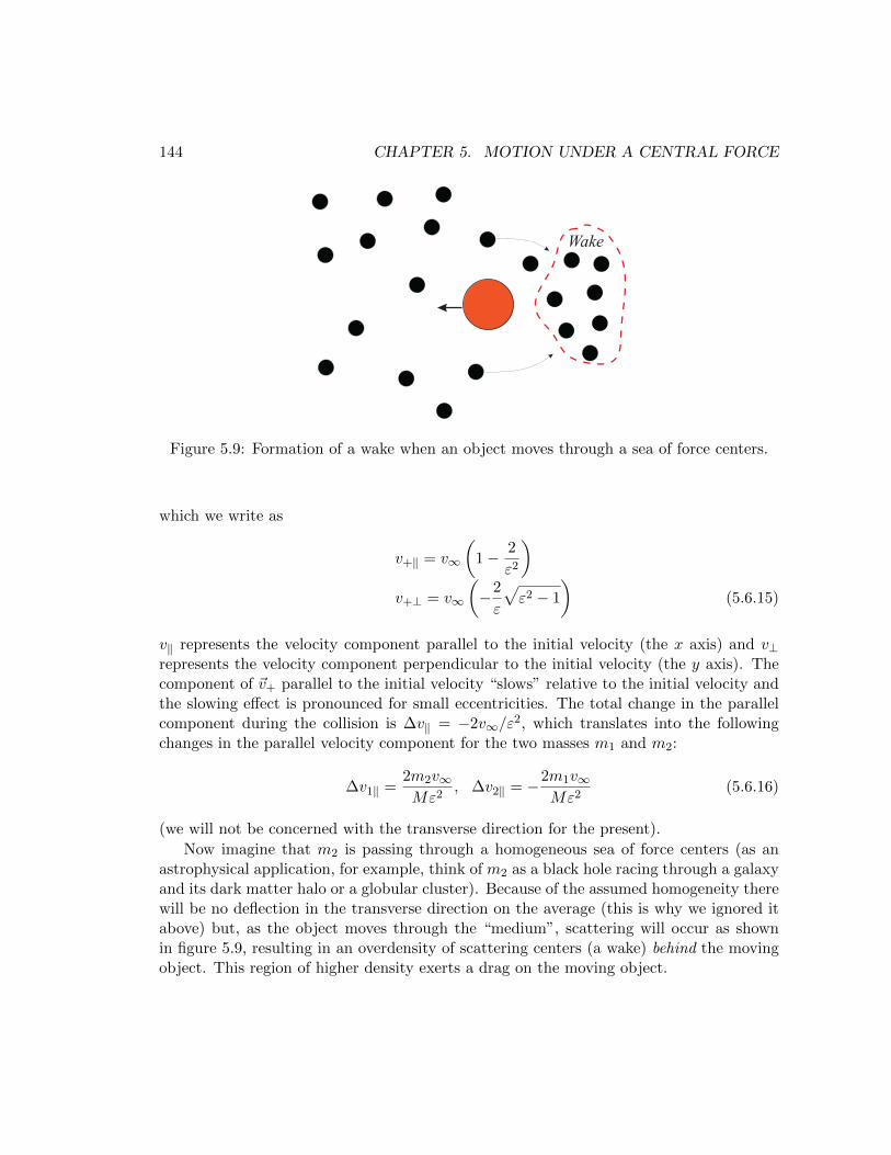
144 CHAPTER 5. MOTION UNDER A CENTRAL FORCE
Wake
Figure 5.9: Formation of a wake when an object moves through a sea of force centers.
which we write as
v+‖ = v∞
(1− 2
ε2
)v+⊥ = v∞
(−2
ε
√ε2 − 1
)(5.6.15)
v‖ represents the velocity component parallel to the initial velocity (the x axis) and v⊥represents the velocity component perpendicular to the initial velocity (the y axis). Thecomponent of ~v+ parallel to the initial velocity “slows” relative to the initial velocity andthe slowing effect is pronounced for small eccentricities. The total change in the parallelcomponent during the collision is ∆v‖ = −2v∞/ε
2, which translates into the followingchanges in the parallel velocity component for the two masses m1 and m2:
∆v1‖ =2m2v∞Mε2
, ∆v2‖ = −2m1v∞Mε2
(5.6.16)
(we will not be concerned with the transverse direction for the present).
Now imagine that m2 is passing through a homogeneous sea of force centers (as anastrophysical application, for example, think of m2 as a black hole racing through a galaxyand its dark matter halo or a globular cluster). Because of the assumed homogeneity therewill be no deflection in the transverse direction on the average (this is why we ignored itabove) but, as the object moves through the “medium”, scattering will occur as shownin figure 5.9, resulting in an overdensity of scattering centers (a wake) behind the movingobject. This region of higher density exerts a drag on the moving object.
5.6. SCATTERING BY A CENTRAL FORCE 145
We now single out ~v2, call it ~vM and its associated mass M . Let the force centers belabeled by by their velocities ~v, along with a distribution function 2πbf(~v)dbd3~v giving thenumber, dN , of force centers with velocities between ~v and ~v + d~v, masses m and impactparameters between b and b + db. The rate at which the mass M encounters these forcecenters is
2πb(v∞λ
)f(~v)dbd3~v (5.6.17)
where λ is the mean distance between them. For each encounter, there is a change invM‖ given by (5.6.16). The average rate of change of ~vM due to encounters with dN forcecenters is therefore
d
(dvM⊥dt
)= 0
d
(dvM‖
dt
)= − 4πµv2
∞λ(m+M)
[1 +
2EL2
µk2
]−1
bf(~v)dbd3~v
= − 4πµv2∞
λ(m+M)
[1 +
µ2v4∞b
2
k2
]−1
bf(~v)dbd3~v (5.6.18)
Perform the b integration from zero up to some maximum value to get
d
(dvM‖
dt
)= − 2πk2
λµ(M +m)v2∞
ln
(1 +
b2maxµ2v4∞
k2
)f(~v)d3~v (5.6.19)
A reasonable choice for bmax is the size of the system of force centers in which the mass Mis moving. In practice, the argument of the natural logarithm is very large and is usuallyreplaced by a constant, Λ2. As v∞ is actually |~vM − ~v| and v⊥ undergoes no change, wecan integrate over the distribution writing the above equation as
d~vMdt≈ − 4πk2
λµ(m+M)ln Λ
∫ vM
0
~vM − ~v|~vM − ~v|3
f(~v)d3~v (5.6.20)
For an isotropic distribution,
d~vMdt≈ − 16π2k2
λµ(M +m)ln Λ
~vM|~vM |3
∫ vM
0f(v)v2dv (5.6.21)
and if the interactions are gravitational then k = G(m+M)µ gives
d~vMdt≈ −16π2G2(m+M)µ
λln Λ
~vM|~vM |3
∫ vM
0f(v)v2dv (5.6.22)
The integral is taken over all force centers in the distribution with speeds up to vM . Theeffect causes a gradual slowing down of the mass M as if it were moving in a viscousfield. However, it has nothing to do with friction and is purely due to the central force,as switching it off by setting k = 0 would elliminate it.9
9Problem: If the central force is repulsive, what sort of effect may one expect? Why?
Chapter 6
Motion in Non-Inertial ReferenceFrames
So far we have examined motion only from the point of view of the “inertial” observer.Recall that while we were discussing Newton’s laws we defined such an observer (frame)as one in which the trajectory of a “free ” body is a straight line. There is some ambiguityhere, as the observer must either know independently of her(is) frame that a body is free,and then determine which frames are inertial, or s(he) must (independently) determinewhether her(is) frame is inertial and subsequently whether the body is “free”. The conceptof a free body is therefore intimately tied with the concept of an inertial frame. Theproblem is more severe when we realize that the ambiguity creeps into the definition of aforce in the second law as that which gives rise to deviations from the first law.
This issue was addressed generally only in the early part of the twentieth centuryby Einstein. We do not here delve into its resolution, but we assume that it is alwayspossible to find a family of inertial frames. However, it may often be impossible for agiven observer to actually occupy such a frame. For example, in order to describe themotion of a particle on the surface of the earth, the most convenient frame is one thatis attached to the earth itself. But the earth rotates both about itself and the sun, andthe entire solar system rotates about the galaxy while also oscillating about the galacticplane. The earth, convenient though it may be as a reference frame, is certainly not aninertial.
6.1 Newton’s second law in an accelerating frame
Since we will assume that inertial frames exist, let us compare our description of motiontwo frames S and S′, in which S is inertial. Suppose that S′ is non-inertial, having an
146
6.2. ROTATING FRAMES 147
acceleration ~a(t) relative to S. It is clear that, instantaneously,
~r′ = ~r − ~R (6.1.1)
where ~r(t) and ~r′(t) represent the positions of a particle, P , relative to S and S′, and ~Ris the position of S′ relative to S at time t. Taking derivatives,
~v′ = ~v − ~vR
~a′ = ~a− ~aR (6.1.2)
Now, Newton’s laws are applicable in the unprimed frame, so if ~F textext is the force actingon the particle at P , its motion, as described in S would be given by Newton’s second law
m~a = ~F ext ⇒ m~a′ = ~F ext −m~aR. = ~F ext + ~f (6.1.3)
(Notice that, if the acceleration of S′ were zero as measured by S, then Newton’s secondlaw would hold in S′ as well. Therefore, all frames moving at a constant velocity relativeto an inertial frame are also inertial.) In general, we must account the additional termf = −m~aR that appears on the right hand side. It has the mechanical dimension of forceand we will refer to it as a “fictitious” force, ~f . One recognizes a fictitious force by thefact that it is multiplied by the mass of the particle itself, so that the acceleration of thebody measured in S′, due to the fictitious force, is independent of its mass,
d2~r′
dt2=
~F ext
m− ~aR. (6.1.4)
In other words: motion under the influence of purely fictitious forces is kinematical (themass, or inertial, of the body plays no role in the equations of motion)! An example ofsuch a force is obviously gravity itself, since the weak equivalence principle ensures thatthe mass appearing on the left hand side of Newton’s equation is the same as the massappearing the the gravitational force law.
6.2 Rotating Frames
In considering the earth itself as a reference frame, the dominant acceleration of an observerfixed relative to the surface of the earth is her(is) centripetal acceleration due to therotation of the earth about its north-south axis. As a special, but nevertheless veryinteresting case, let us describe the motion of a body in a frame that is rotating withrespect to an inertial frame, but not translating relative to it. As before, let S be aninertial frame and S′ be a non-inertial frame, rotating about some axis OP as shown infigure (6.1). Any vector ~A may be described in S or S′
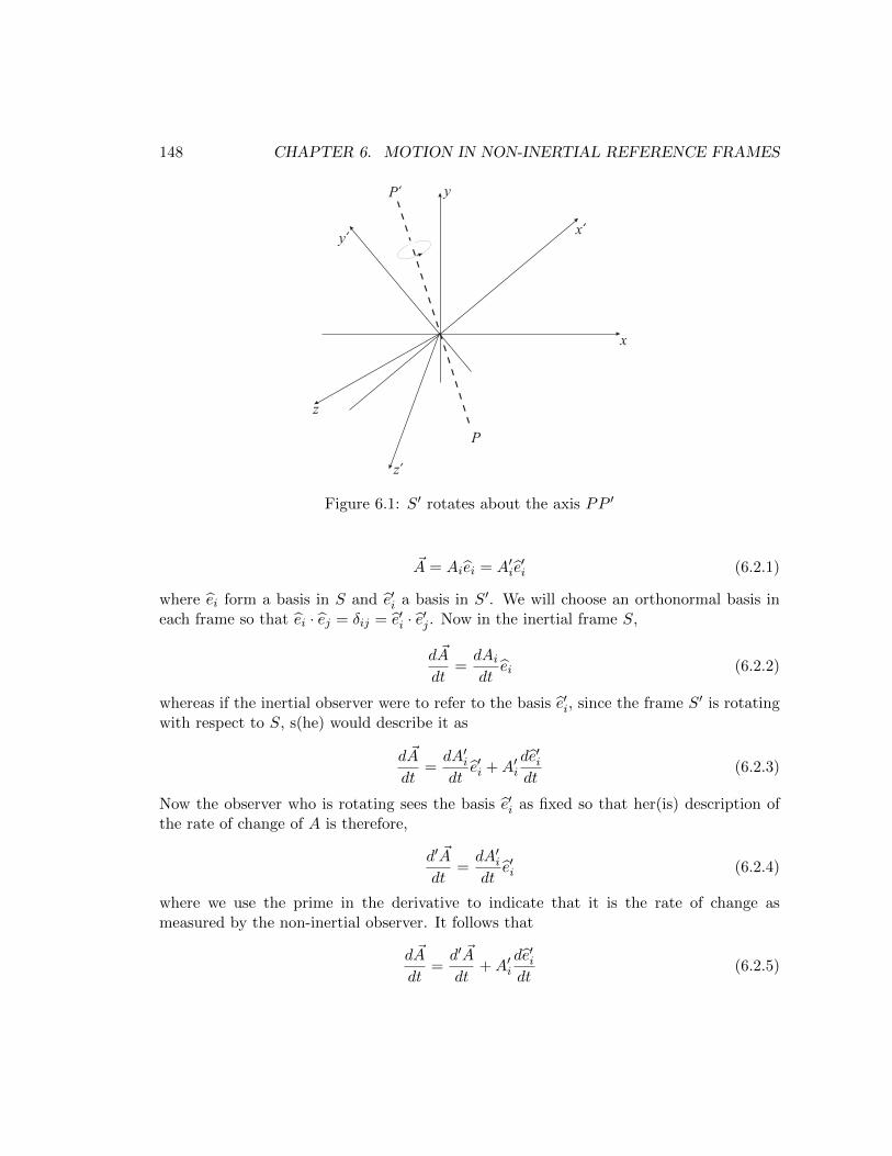
148 CHAPTER 6. MOTION IN NON-INERTIAL REFERENCE FRAMES
x
x’
y
y’
z
z’
P’
P
Figure 6.1: S′ rotates about the axis PP ′
~A = Aiei = A′ie′i (6.2.1)
where ei form a basis in S and e′i a basis in S′. We will choose an orthonormal basis ineach frame so that ei · ej = δij = e′i · e′j . Now in the inertial frame S,
d ~A
dt=dAidt
ei (6.2.2)
whereas if the inertial observer were to refer to the basis e′i, since the frame S′ is rotatingwith respect to S, s(he) would describe it as
d ~A
dt=dA′idt
e′i +A′ide′idt
(6.2.3)
Now the observer who is rotating sees the basis e′i as fixed so that her(is) description ofthe rate of change of A is therefore,
d′ ~A
dt=dA′idt
e′i (6.2.4)
where we use the prime in the derivative to indicate that it is the rate of change asmeasured by the non-inertial observer. It follows that
d ~A
dt=d′ ~A
dt+A′i
de′idt
(6.2.5)
6.2. ROTATING FRAMES 149
Let us concentrate on the difference between the derivatives: A′ide′i/dt. Because the rate
of change of each basis vector in S′ is itself a vector, it can be expanded in the S′ basis,i.e.,
de′idt
= aij e′j (6.2.6)
But since the basis vectors in S′ are orthonormal
e′i · e′j = δij ⇒de′idt· e′j = −e′i ·
de′jdt⇒ aij = −aji, ∀ i, j ∈ 1, 2, 3. (6.2.7)
This means that the matrix aij is antisymmetric, and therefore has only 3 independentcomponents (as opposed to nine for a general real 3× 3 matrix). We could write it as
a =
0 a12 a13
−a12 0 a23
−a13 −a23 0
(6.2.8)
Define the vector ~ω with components
[~ω]i =1
2εijkajk (6.2.9)
in the S basis. Inverting this definition for aij , we find
εlmiωi =1
2εlmiεijkajk =
1
2(δljδmk − δlkδmj)ajk = alm (6.2.10)
oralm = εlmkωk, (6.2.11)
where we use the fact that a is antisymmetric. Then
de′idt
= aij e′j = εijkωke
′j = ~ω × e′i (6.2.12)
The last step is not obvious, but it is straightforward to prove. Let the basis vectors begiven by
[e′i]k = δik (6.2.13)
then consider each component
de′1dt
= ω3e′2 − ω2e
′3 = (0, ω3,−ω2) = ~ω × e′1
150 CHAPTER 6. MOTION IN NON-INERTIAL REFERENCE FRAMES
de′2dt
= ω1e′3 − ω3e
′1 = (−ω3, 0, ω1) = ~ω × e′2
de′3dt
= ω2e′1 − ω1e
′2 = (ω2,−ω1, 0) = ~ω × e′3 (6.2.14)
It follows that (6.2.5) can be written in the form
d ~A
dt=d′ ~A
dt+ ~ω × ~A (6.2.15)
or, viewed as an operator, the derivative transforms from one frame to the other as
d
dt. . . =
[d′
dt+ ω ×
]. . . . (6.2.16)
This general result is valid for any vector ~A1 and in particular for the position vector of aparticle, i.e.,
d~r
dt=d′~r
dt+ ~ω × ~r (6.2.17)
If we take another derivative, to obtain the acceleration in the S frame,
d2~r
dt2=
d
dt
[d′~r
dt+ ~ω × ~r
]=
d′
dt
[d′~r
dt+ ~ω × ~r
]+ ω ×
[d′~r
dt+ ~ω × ~r
](6.2.18)
we findd2~r
dt2=d′2~r
dt2+ 2~ω × d′~r
dt+ ~ω × (~ω × ~r) +
d′~ω
dt× ~r (6.2.19)
This is called Coriolis’ theorem. All the time derivatives on the right are relative to therotating observer. This means that if the particle with position vector ~r is subject to aforce ~F as measured in S, then Newton’s second law reads
md2~r
dt2= ~F (6.2.20)
or, written in the rotating frame,
d′2~r
dt2+ 2~ω × d′~r
dt+ ~ω × (~ω × ~r) +
d′~ω
dt× ~r =
~F
m. (6.2.21)
1Notice thatd~ω
dt=d′~ω
dtsince ~ω × ~ω = 0.
6.3. MOTION NEAR THE SURFACE OF THE EARTH. 151
It follows, according to (6.1.3), that we must associate
~f = −m[2~ω × d′~r
dt+ ~ω × (~ω × ~r) +
d′~ω
dt× ~r]
(6.2.22)
with the fictitious force that appears to act on the particle when it is described in thenon-inertial frame S′. The first term is called the Corriolis force. The second is thecentrifugal force and the last term, which turns out to have no particular name, isrelevant only if the angular velocity of S′ is changing in time. This is because, as we arguebelow, ~ω is the instantaneous angular velocity of S′ relative to S.
Although ~ω was introduced in somewhat of an ad hoc manner in the previous section,it can easily be assigned a physical significance. To do so, we must first show that itpossesses the transformation properties under rigid rotations that would make it a vector.But this is obvious because from (6.2.6) it follows that aij transforms as two copies of avector (i.e., is a rank two tensor),
a′ij = RilRjmalm (6.2.23)
and, because the Levi-Civita symbol is a rank three tensor, (6.2.9) ensures that ~ω trans-forms as a vector. It is even easier to see that ~ω is the angular velocity of the frame S′.Let ~A be any one of the basis vectors in the S′ frame. Since the basis vectors e′i are notmoving relative to the S′ observer, d′e′i/dt = 0. We then have
de′idt
= ~ω × e′i, (6.2.24)
which is precisely the equation for a vector that is rotating with an angular velocity ~ω.
6.3 Motion near the surface of the earth.
For an observer fixed relative to the surface of the rotating earth, it is natural to apply notNewton’s second law, but Corriolis’ theorem in describing the motion of a body. Thus,the effective equations of motion take into account the fictitious forces that must be addedto compensate for her(is) rotation,
d′2~r
dt2+ 2~ω × d′~r
dt+ ~ω × (~ω × ~r) +
d′~ω
dt× ~r =
~F
m+ ~g (6.3.1)
where we have restricted our attention to bodies moving close to the surface of the earth(at heights that are small compared to the earth’s radius) and ~F now incorporates allforces apart from the gravitational pull of the earth on the body.
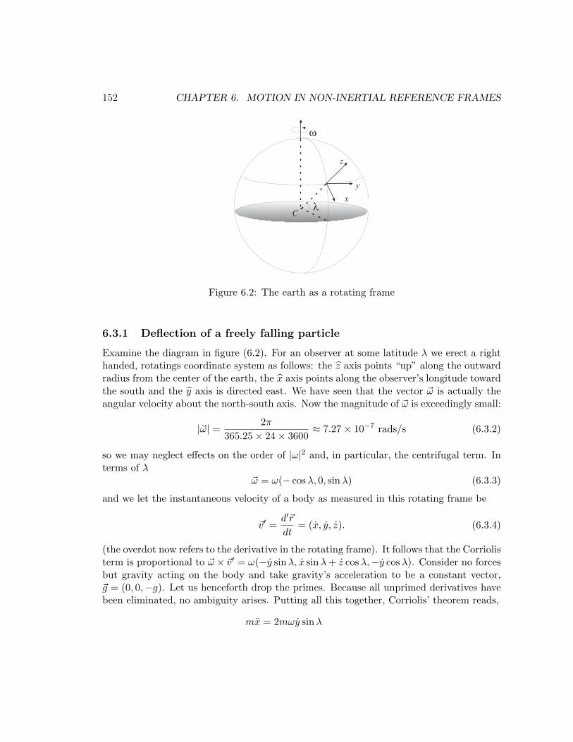
152 CHAPTER 6. MOTION IN NON-INERTIAL REFERENCE FRAMES
x
y
z
Cl
w
Figure 6.2: The earth as a rotating frame
6.3.1 Deflection of a freely falling particle
Examine the diagram in figure (6.2). For an observer at some latitude λ we erect a righthanded, rotatings coordinate system as follows: the z axis points “up” along the outwardradius from the center of the earth, the x axis points along the observer’s longitude towardthe south and the y axis is directed east. We have seen that the vector ~ω is actually theangular velocity about the north-south axis. Now the magnitude of ~ω is exceedingly small:
|~ω| = 2π
365.25× 24× 3600≈ 7.27× 10⁻⁷ rads/s (6.3.2)
so we may neglect effects on the order of |ω|2 and, in particular, the centrifugal term. Interms of λ
~ω = ω(− cosλ, 0, sinλ) (6.3.3)
and we let the instantaneous velocity of a body as measured in this rotating frame be
~v′ =d′~r
dt= (x, y, z). (6.3.4)
(the overdot now refers to the derivative in the rotating frame). It follows that the Corriolisterm is proportional to ~ω× ~v′ = ω(−y sinλ, x sinλ+ z cosλ,−y cosλ). Consider no forcesbut gravity acting on the body and take gravity’s acceleration to be a constant vector,~g = (0, 0,−g). Let us henceforth drop the primes. Because all unprimed derivatives havebeen eliminated, no ambiguity arises. Putting all this together, Corriolis’ theorem reads,
mx = 2mωy sinλ
6.3. MOTION NEAR THE SURFACE OF THE EARTH. 153
my = −2mω[x sinλ+ z cosλ]
mz = −mg + 2mωy cosλ (6.3.5)
If the initial velocity has no component in the east-west or north-south direction thenevidently both x and y will be of order ω. This means that we can approximate theequations above by
mx ≈ 0
my ≈ −2mωz cosλ
mz ≈ −mg (6.3.6)
to be consistent with our neglect of terms that are second order in ω, such as the centrifugalterm. This system of equations is easy to solve: the last equation says that
z(t) = z0 −1
2gt2 (6.3.7)
assuming that z0 = 0. Inserted into the second equation this gives
y = y0 +1
3ωgt3 cosλ (6.3.8)
and, evidently, x = x0. Notice that there is deflection of the falling body along the easterlydirection,2 of magnitude
∆y =1
3ωgt3 cosλ (6.3.9)
The deflection is maximum at the equator and vanishes at the pole, in agreement withwhat one would naturally expect. If the body falls through a height h then
t =
√2h
g⇒ ∆y =
1
3ω cosλ
√8h3
g(6.3.10)
The result does not depend on the mass of the body because the forces causing thedeflection are fictitious.
2Problem: Erect a suitable right handed coordinate system in the southern hemisphere and show thata deflection of the same magnitude occurs in the westerly direction.
154 CHAPTER 6. MOTION IN NON-INERTIAL REFERENCE FRAMES
6.3.2 Motion of a projectile
Take a projectile that is fired from the origin in the easterly direction and making an angleof α with the y−axis, so that the initial conditions read:
~r0 = 0, ~v0 = v0(0, cosα, sinα) (6.3.11)
Because v0x = 0, x will always be of order ω and because y is driven by an omega dependentforce, changes to y will be of order ω, that is, y = v0 cosα +O(ω). Thus, up to the firstorder in ω our equations in (6.3.5) read
mx ≈ 2mωv0 cosα sinλ
my ≈ −2mωz cosλ
mz = −mg + 2mωv0 cosα cosλ (6.3.12)
The first and last equations are immediately solved:
x(t) ≈ ωv0t2 cosα sinλ
z(t) ≈ v0t sinα+
(−1
2g + ωv0 cosα cosλ
)t2 (6.3.13)
Up to the first order, only the first term in z(t) is relevant in the equation for y. Thesecond term would contribute to O(ω2). Therefore
y ≈ −2ω cosλ(v0 sinα− gt) (6.3.14)
which gives
y(t) = v0 cosα− 2ω
(v0t sinα− 1
2gt2)
cosλ
y(t) = v0 cosαt− ω(v0t
2 sinα− 1
3gt3)
cosλ (6.3.15)
Now the deflection is southerly and given as a function of time by (6.3.13). To find thetotal deflection we require the time taken by the projectile to strike the earth, which isthe non-vanishing solution of z(t) = 0,
t =2v0 sinα
g − 2ωv0 cosα cosλ≈ 2v0 sinα
g
[1 +
2ωv0
gcosα cosλ+ . . .
](6.3.16)
6.3. MOTION NEAR THE SURFACE OF THE EARTH. 155
The total deflection, to order ω is then
∆x =4ωv3
0
g2sinλ cosα sin2 α (6.3.17)
It is vanishing for a projectile fired along the equator.If the projectile is fired in the southerly direction and making an angle of α with the
x− axis, our initial conditions would read
~r0 = 0, ~v0 = v0(cosα, 0, sinα) (6.3.18)
Applying the same arguments as in the previous example, Corriolis’ theorem approximatedup to the first order in ω gives
x = 0
y = −2ω[x sinλ+ z cosλ]
z = −g (6.3.19)
With our initial conditions,
x(t) = v0t cosα, z(t) = v0t sinα− 1
2gt2 (6.3.20)
andy = −2ω[v0 cosα sinλ+ (v0 sinα− gt) cosλ] (6.3.21)
Integrating this equation, subject to the initial conditions we find
y(t) = −2ω
[v0t sin(α+ λ)− 1
2gt2 cosλ
](6.3.22)
and
y(t) = −ω[v0t
2(sin(α+ λ)− 1
3gt3 cosλ
](6.3.23)
When the time for the projectile to strike the earth,
t =2v0 sinα
g, (6.3.24)
is substituted into the expression for y(t) gives the total deflection as
∆y = −4ωv30
3g2sin2 α (sinα cosλ+ 3 cosα sinλ) . (6.3.25)
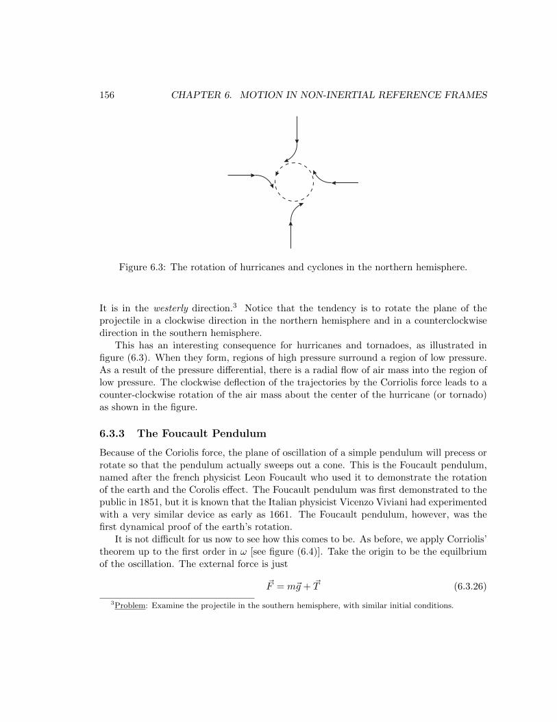
156 CHAPTER 6. MOTION IN NON-INERTIAL REFERENCE FRAMES
Figure 6.3: The rotation of hurricanes and cyclones in the northern hemisphere.
It is in the westerly direction.3 Notice that the tendency is to rotate the plane of theprojectile in a clockwise direction in the northern hemisphere and in a counterclockwisedirection in the southern hemisphere.
This has an interesting consequence for hurricanes and tornadoes, as illustrated infigure (6.3). When they form, regions of high pressure surround a region of low pressure.As a result of the pressure differential, there is a radial flow of air mass into the region oflow pressure. The clockwise deflection of the trajectories by the Corriolis force leads to acounter-clockwise rotation of the air mass about the center of the hurricane (or tornado)as shown in the figure.
6.3.3 The Foucault Pendulum
Because of the Coriolis force, the plane of oscillation of a simple pendulum will precess orrotate so that the pendulum actually sweeps out a cone. This is the Foucault pendulum,named after the french physicist Leon Foucault who used it to demonstrate the rotationof the earth and the Corolis effect. The Foucault pendulum was first demonstrated to thepublic in 1851, but it is known that the Italian physicist Vicenzo Viviani had experimentedwith a very similar device as early as 1661. The Foucault pendulum, however, was thefirst dynamical proof of the earth’s rotation.
It is not difficult for us now to see how this comes to be. As before, we apply Corriolis’theorem up to the first order in ω [see figure (6.4)]. Take the origin to be the equilbriumof the oscillation. The external force is just
~F = m~g + ~T (6.3.26)
3Problem: Examine the projectile in the southern hemisphere, with similar initial conditions.
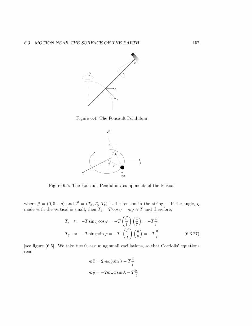
6.3. MOTION NEAR THE SURFACE OF THE EARTH. 157
z
x
y
w
Figure 6.4: The Foucault Pendulum
y
z
x
T
mg
f
hl
l’
Figure 6.5: The Foucault Pendulum: components of the tension
where ~g = (0, 0,−g) and ~T = (Tx, Ty, Tz) is the tension in the string. If the angle, ηmade with the vertical is small, then Tz = T cos η = mg ≈ T and therefore,
Tx ≈ −T sin η cosϕ = −T(l′
l
)(xl′
)= −T x
l
Ty ≈ −T sin η sinϕ = −T(l′
l
)(yl′
)= −T y
l(6.3.27)
[see figure (6.5]. We take z ≈ 0, assuming small oscillations, so that Corriolis’ equationsread
mx = 2mωy sinλ− T xl
my = −2mωx sinλ− T yl
158 CHAPTER 6. MOTION IN NON-INERTIAL REFERENCE FRAMES
mz = 2mωy cosλ−mg + T (6.3.28)
It is convenient to define the variable u = x+ iy and write the first two equations as thefollowing complex equation in u
mu = −2imωu sinλ− T ul
(6.3.29)
which can be written in the form of the linear equation
mu+ iβu+ α2u = 0 (6.3.30)
where β = 2mω sinλ and α2 = T/l. The roots of the auxiliary equation are
λ± = − i
2m
[β ±
√β2 + 4mα2
](6.3.31)
Define the quantities ω0 = α/√m =
√T/ml ≈
√g/l, which is independent of the earth’s
rotation, and γ = β/2m = ω sinλ, which vanishes if ω = 0. The general solution is of theform
u(t) = e−iγt[Aei√ω20+γ2 +Be−i
√ω20+γ2
](6.3.32)
To understand it, imagine for a moment that the earth does not rotate, i.e., that ω = 0,then our solution reads
u0(t) = Aeiω0t +Be−iω0t (6.3.33)
which represents a simple oscillation of frequency ω0. But, when γ is small (we areinterested only in terms up to the first order in ω), we can neglect the γ2 occurring insidethe radicals in (6.3.32) so that
u(t) ≈ e−iγtu0(t). (6.3.34)
Recalling that u(t) = x(t) + iy(t), this can be put into the suggestive formx(t)
y(t)
≈ cos γt sin γt
− sin γt cos γt
x0(t)
y0(t)
, (6.3.35)
showing that the plane of the simple oscillations that would occur in the absence of theearth’s rotation is subject to a time dependent rotation at constant angular velocity γ =ω sinλ.
Chapter 7
Rigid Bodies
A rigid body is defined as a system of particles for which the relative distance betweenany two particles is constant. There are, of course, no truly rigid bodies in nature becausebeing rigid implies that the body cannot admit any deformations whatsoever, and weknow of no such system of particles: every body may be deformed, at least minimally, bythe application of external forces. The existence of purely rigid bodies is also prohibitedby special relativity because a truly rigid body would transmit information at an infinitespeed, which contradicts the postulate that no signal can travel faster than the speed oflight.
How many degrees of freedom would a rigid body possess? Consider any one particlein the rigid body. To locate this particle relative to any coordinate system requires threecoordinates (or one position vector). Now consider a second particle within the body:because its distance from the first is fixed it must lie on the surface of a sphere of a fixedradius from the first, so we now require only two coordinates to locate this particle. Athird particle is at fixed distances from the first and the second particles, so it lies on thecurve of intersection of two spheres centered about them. This calls for just one additionalcoordinate to locate its position. Once the positions of the first three particles are fixedthe positions of the remaining particles are completely determined in terms of them by theconstraints, therefore a rigid body in three dimensions possesses six degrees of freedom.1
Solids admit strong interactions between their elementary constituents that do a prettygood job of resisting deformation and “rigidity” entails taking those inter-molecular inter-actions resisting deformations to be effectively infinite or, more realistically, much largerthan the external applied forces. Our objective in this chapter is to describe the motionin three dimensions of a system of particles that is effectively rigid.
1Problem: Repeat this argument to show that in D dimensions a rigid body will have D(D+1)2
degreesof freedom.
159
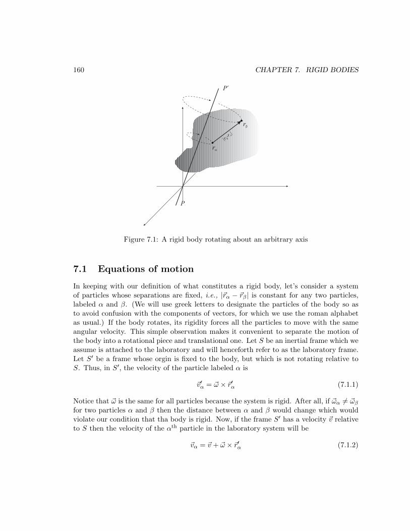
160 CHAPTER 7. RIGID BODIES
ra
rb
|r-r
|b
a
P
P’
Figure 7.1: A rigid body rotating about an arbitrary axis
7.1 Equations of motion
In keeping with our definition of what constitutes a rigid body, let’s consider a systemof particles whose separations are fixed, i.e., |~rα − ~rβ| is constant for any two particles,labeled α and β. (We will use greek letters to designate the particles of the body so asto avoid confusion with the components of vectors, for which we use the roman alphabetas usual.) If the body rotates, its rigidity forces all the particles to move with the sameangular velocity. This simple observation makes it convenient to separate the motion ofthe body into a rotational piece and translational one. Let S be an inertial frame which weassume is attached to the laboratory and will henceforth refer to as the laboratory frame.Let S′ be a frame whose orgin is fixed to the body, but which is not rotating relative toS. Thus, in S′, the velocity of the particle labeled α is
~v′α = ~ω × ~r′α (7.1.1)
Notice that ~ω is the same for all particles because the system is rigid. After all, if ~ωα 6= ~ωβfor two particles α and β then the distance between α and β would change which wouldviolate our condition that tha body is rigid. Now, if the frame S′ has a velocity ~v relativeto S then the velocity of the αth particle in the laboratory system will be
~vα = ~v + ~ω × ~r′α (7.1.2)
7.2. THE INERTIA TENSOR 161
The total momentum of the system is therefore
~P =∑α
mα~vα = M~v + ~ω ×∑α
mα~r′α (7.1.3)
where M =∑
αmα is the total mass of the body and
d~P
dt= M
d~v
dt+∑α
mαd
dt(~ω × ~r′α) = ~F ext. (7.1.4)
If the origin of S′ is located at the center of mass then the second term is clearly vanishingand the equation says that the center of mass moves as a particle of mass equal to themass of the body and subject to the total external force to which the body is subjected.This equation says nothing about the rotation of the body about the center of mass.
From another point of view, imagine yet another frame S′′ whose origin coincides withthat of S′ but which is rotating with the body. Because their origins coincide, the positionof the αth particle in the body with respect to S′′ is just ~r′α but, with respect to S′′ everyparticle is at rest, therefore
d′~r′αdt
= 0⇒ d~r′αdt− ~ω × ~r′α = 0 (7.1.5)
according to (6.2.17). But if ~r is the position of S′ relative to the laboratory frame S,then ~rα = ~r + ~r′α and
~vα = ~v +d~r′αdt
= ~v + ~ω × ~r′α (7.1.6)
which is the same, of course, as (7.1.2). This leads to the equations of motion in (7.1.5).
7.2 The Inertia Tensor
The equations of motion in (7.1.5) split naturally into translational and rotational pieces.So do the kinetic energy and angular momentum as we now see. The kinetic energy of thebody is the sum of kinetic energies of its constituents, so
K =1
2
∑α
mα~v2α =
1
2
∑α
mα(~v + ~ω × ~r′α)2 (7.2.1)
Expanding the square,
K =1
2
[M~v2 + 2
∑α
mα~v · (~ω × ~r′α) +∑α
mα(~ω × ~r′α)2
]. (7.2.2)
162 CHAPTER 7. RIGID BODIES
If we take S′ (commonly referred to as the “body system”) to lie at the center of mass ofthe rigid body then the second term vanishes because
∑αmα~r
′α ≡ 0. On the other hand,
(~ω × ~r′α) · (~ω × ~r′α) = εijkεipqωjr′α,kωpr
′α,q
= ~ω2~r′2α − (~ω · ~r′α)2 (7.2.3)
giving
K =1
2M~v2
cm + Icmij ωiωj (7.2.4)
where
Iij =∑α
mα(~r′2α δij − ~r′α,i~r′α,j) (7.2.5)
is called the Inertia Tensor of the rigid body. The Kinetic energy in (7.2.4) breaks upinto a translational piece, which is just the translational kinetic energy of the center ofmass, behaving as a particle having the entire mass of the body, and a rotational piece,which is the kinetic energy of the rigid body about the center of mass and is determined bythe angular velocity and the inertia tensor. Notice that while the definition of the inertiatensor is quite generally given by (7.2.5), the simplified expression for the kinetic energydepends on the fact that the body system has its origin at the center of mass. Therefore,in that expression, we have labeled the inertia tensor by the superscript “cm” (for ‘centerof mass”). That the inertia tensor is a rank two, symmetric tensor is clear by inspection.
The angular momentum of the rigid body can also be written in terms of the inertiatensor. Thus,
~L =∑α
~rα × ~pα =∑α
mα(~r + ~r′α)× (~v + ~ω × ~r′α) (7.2.6)
Again, if the origin of S′ is located at the center of mass, we could neglect all termsin which a sum of the form
∑αmα~r
′α appears, because this sum vanishes identically by
definition. It follows that the expression for the angular momentum on the right handside expands into
~L = M~rcm × ~vcm +∑α
mα~r′α × (~ω × ~r′α) (7.2.7)
or, in components,
Li = [~rcm × ~P ]i + Icmij ωj (7.2.8)
which is naturally interpreted as the angular momentum of the center of mass about Splus the angular momentum of the body around the center of mass. Once again, the latteris determined by the inertia tensor.
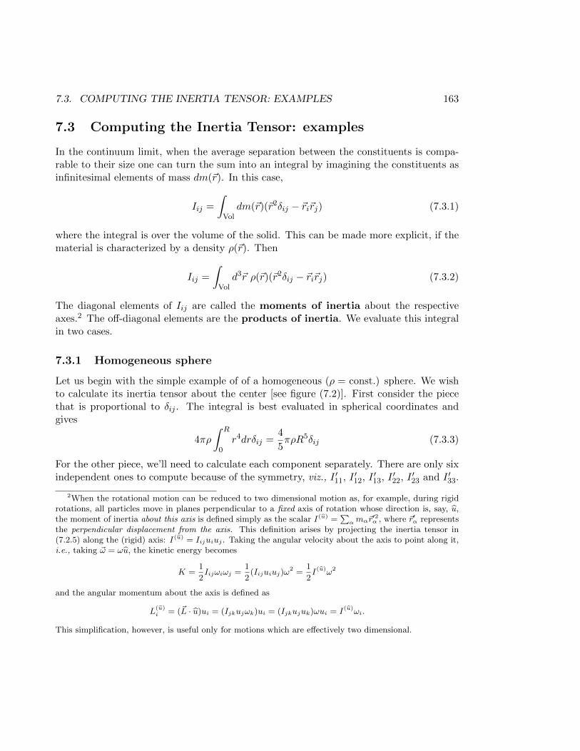
7.3. COMPUTING THE INERTIA TENSOR: EXAMPLES 163
7.3 Computing the Inertia Tensor: examples
In the continuum limit, when the average separation between the constituents is compa-rable to their size one can turn the sum into an integral by imagining the constituents asinfinitesimal elements of mass dm(~r). In this case,
Iij =
∫Vol
dm(~r)(~r2δij − ~ri~rj) (7.3.1)
where the integral is over the volume of the solid. This can be made more explicit, if thematerial is characterized by a density ρ(~r). Then
Iij =
∫Vol
d3~r ρ(~r)(~r2δij − ~ri~rj) (7.3.2)
The diagonal elements of Iij are called the moments of inertia about the respectiveaxes.2 The off-diagonal elements are the products of inertia. We evaluate this integralin two cases.
7.3.1 Homogeneous sphere
Let us begin with the simple example of of a homogeneous (ρ = const.) sphere. We wishto calculate its inertia tensor about the center [see figure (7.2)]. First consider the piecethat is proportional to δij . The integral is best evaluated in spherical coordinates andgives
4πρ
∫ R
0r4drδij =
4
5πρR5δij (7.3.3)
For the other piece, we’ll need to calculate each component separately. There are only sixindependent ones to compute because of the symmetry, viz., I ′11, I ′12, I ′13, I ′22, I ′23 and I ′33.
2When the rotational motion can be reduced to two dimensional motion as, for example, during rigidrotations, all particles move in planes perpendicular to a fixed axis of rotation whose direction is, say, u,the moment of inertia about this axis is defined simply as the scalar I(u) =
∑αmα~r
′2α , where ~r′α represents
the perpendicular displacement from the axis. This definition arises by projecting the inertia tensor in(7.2.5) along the (rigid) axis: I(u) = Iijuiuj . Taking the angular velocity about the axis to point along it,i.e., taking ~ω = ωu, the kinetic energy becomes
K =1
2Iijωiωj =
1
2(Iijuiuj)ω
2 =1
2I(u)ω2
and the angular momentum about the axis is defined as
L(u)i = (~L · u)ui = (Ijkujωk)ui = (Ijkujuk)ωui = I(u)ωi.
This simplification, however, is useful only for motions which are effectively two dimensional.
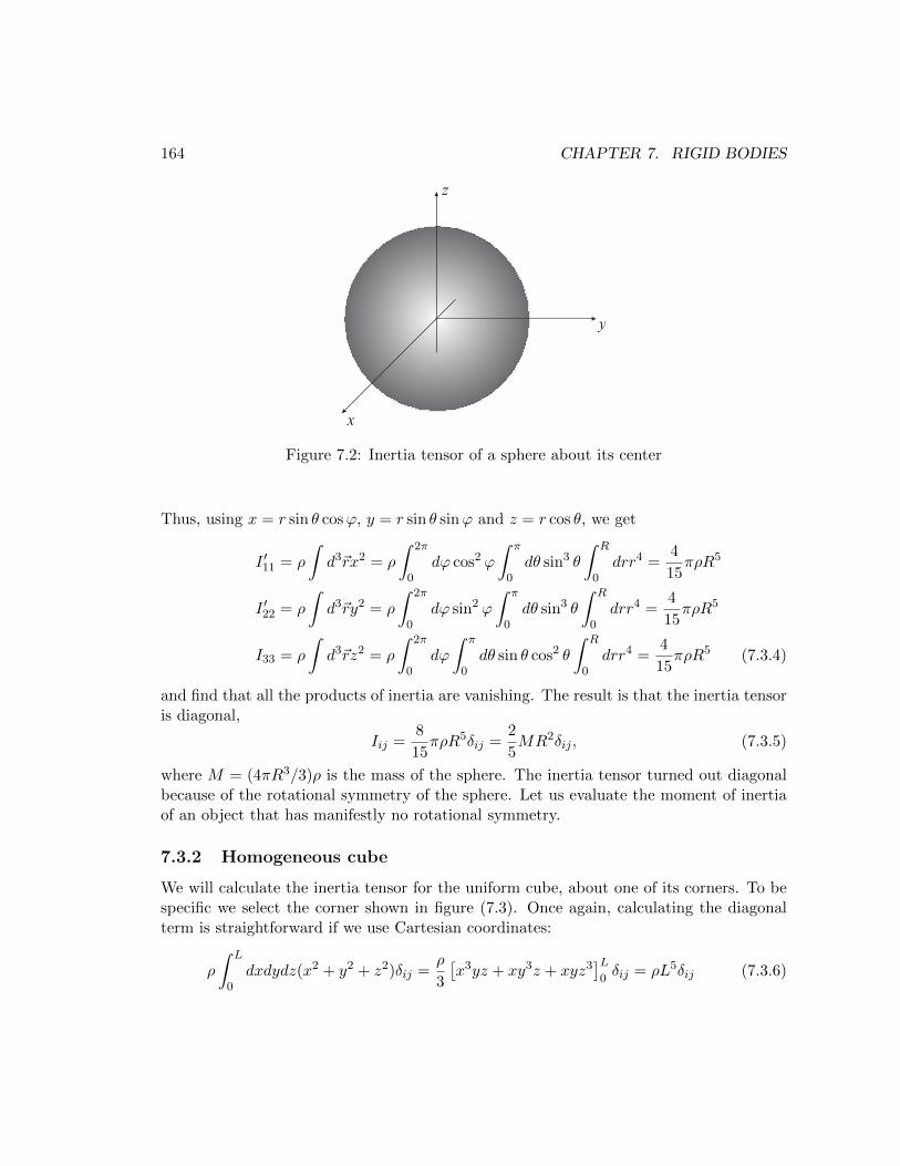
164 CHAPTER 7. RIGID BODIES
x
y
z
Figure 7.2: Inertia tensor of a sphere about its center
Thus, using x = r sin θ cosϕ, y = r sin θ sinϕ and z = r cos θ, we get
I ′11 = ρ
∫d3~rx2 = ρ
∫ 2π
0dϕ cos2 ϕ
∫ π
0dθ sin3 θ
∫ R
0drr4 =
4
15πρR5
I ′22 = ρ
∫d3~ry2 = ρ
∫ 2π
0dϕ sin2 ϕ
∫ π
0dθ sin3 θ
∫ R
0drr4 =
4
15πρR5
I33 = ρ
∫d3~rz2 = ρ
∫ 2π
0dϕ
∫ π
0dθ sin θ cos2 θ
∫ R
0drr4 =
4
15πρR5 (7.3.4)
and find that all the products of inertia are vanishing. The result is that the inertia tensoris diagonal,
Iij =8
15πρR5δij =
2
5MR2δij , (7.3.5)
where M = (4πR3/3)ρ is the mass of the sphere. The inertia tensor turned out diagonalbecause of the rotational symmetry of the sphere. Let us evaluate the moment of inertiaof an object that has manifestly no rotational symmetry.
7.3.2 Homogeneous cube
We will calculate the inertia tensor for the uniform cube, about one of its corners. To bespecific we select the corner shown in figure (7.3). Once again, calculating the diagonalterm is straightforward if we use Cartesian coordinates:
ρ
∫ L
0dxdydz(x2 + y2 + z2)δij =
ρ
3
[x3yz + xy3z + xyz3
]L0δij = ρL5δij (7.3.6)
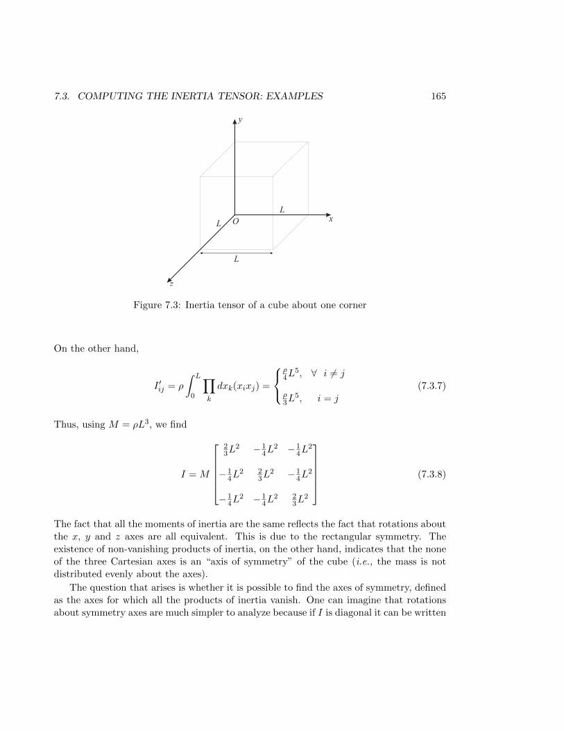
7.3. COMPUTING THE INERTIA TENSOR: EXAMPLES 165
x
y
z
O
L
L
L
Figure 7.3: Inertia tensor of a cube about one corner
On the other hand,
I ′ij = ρ
∫ L
0
∏k
dxk(xixj) =
ρ4L
5, ∀ i 6= j
ρ3L
5, i = j(7.3.7)
Thus, using M = ρL3, we find
I = M
23L
2 −14L
2 −14L
2
−14L
2 23L
2 −14L
2
−14L
2 −14L
2 23L
2
(7.3.8)
The fact that all the moments of inertia are the same reflects the fact that rotations aboutthe x, y and z axes are all equivalent. This is due to the rectangular symmetry. Theexistence of non-vanishing products of inertia, on the other hand, indicates that the noneof the three Cartesian axes is an “axis of symmetry” of the cube (i.e., the mass is notdistributed evenly about the axes).
The question that arises is whether it is possible to find the axes of symmetry, definedas the axes for which all the products of inertia vanish. One can imagine that rotationsabout symmetry axes are much simpler to analyze because if I is diagonal it can be written
166 CHAPTER 7. RIGID BODIES
in the form I = Iiδij (no sum) and then the kinetic energy reduces to
K =1
2Iijωiωj =
1
2
∑i
Iiω2i (7.3.9)
andLi = Iijωj = Iiωi (7.3.10)
We see that the purely mathematical problem of diagonalizing a symmetric matrix isactually in this case the physical problem of determining the axes of symmetry of thebody.
The “axes of symmetry” are just the eigenvectors of the inertia tensor. The eigenvaluesare called the “principal moments of inertia” and the eigenvectors are called the “principalaxes”. In many systems of high symmetry, the principal axes are determined by inspection.For the cube they are not so evident, so let us determine the principal axes, passing throughthe origin. We must diagonalize the matrix
I =
23α −1
4α −14α
−14α
23α −1
4α
−14α −1
4α23α
, α = ML2 (7.3.11)
The secular equation, |I − λ1| = 0 is(2
3α− λ
)2
− α3
32− 3
16α2
(2
3α− λ
)= 0 (7.3.12)
and one can easily check that the eigenvalues are
λ =
1
6α,
11
12α
(7.3.13)
where the second is degenerate. The diagonalized inertia tensor is then
ID =
16α 0 0
0 1112α 0
0 0 1112α
(7.3.14)
To find the principal axes (the eigenvectors), we use the eigenvalue equation (vn =(un, vn, wn))
I vn = λnvn (7.3.15)
7.3. COMPUTING THE INERTIA TENSOR: EXAMPLES 167
which gives
2α
3un −
α
4vn −
α
4wn = λnun
−α4un +
2α
3vn −
α
4wn = λnvn
−α4un −
α
4vn +
2α
3wn = λnwn (7.3.16)
For λn = α/6 we find
vα/6 =1√3
111
(7.3.17)
For the degenerate eigenvalue, 11α/12, the principal axes lie in the plane
u+ v + w = 0, (7.3.18)
passing through the origin with normal given precisely by vα/6. Thus 11α/12 is themoment of inertia of a cube rotating about any axis passing through the origin and in theplane perpendicular to vα/6. It should be obvious that the principal axes for the cube areobtainable by a rotation of the original axes. We now prove that this is true in general:the inertia tensor may always be diagonalized by a rotation of the original system.
Consider a rotation of the original coordinate system so that
~rα → ~r′α = R~rα (7.3.19)
Because I is a second rank tensor, under the rotation above it transforms as
Iij → I ′ij =∑lm
RilRjmIlm (7.3.20)
or
I = R I RT . (7.3.21)
Now what condition must be satisfied so that I ′ij is diagonal? We should have
I ′iδij =∑lm
RilRjmIlm ⇒∑j
I ′iδijRTnj =
∑jlm
RilRTnjRjmIlm (7.3.22)
So we see that
I ′iRTni =
∑lm
RilδnmIlm =∑l
RilIln (7.3.23)
168 CHAPTER 7. RIGID BODIES
and therefore ∑l
Ril(Iln − I ′iδln) = 0 (7.3.24)
which is possible if and only if the secular equation |I − Ii1| = 0 holds because |R| = 1.This is the eigenvalue condition which yields the principal moments of inertia. Thereforethe principal axes are determined by a rotation of the original system.
Let us return to the example of the cube and find the rotation matrix that takes thex− axis to the diagonal principal axis of the cube. We will see that it diagonalizes theinertia tensor obtained before. We want to take the unit vector x = (1, 0, 0) to the unitvector
x′ =1√3
(1, 1, 1)
and for the y′ and z′ axes we choose any axes in the plane perpendicular to x′. Forinstance, choose
y′ =1√2
(−1, 1, 0) (7.3.25)
and
z′ = x′ × y′ = 1√6
(−1,−1, 2) (7.3.26)
Recalling that the basis vectors transform as
Rikek = e′i (7.3.27)
we can take an inner product of both sides with ej to get
Rikek · ej = Rikδkj = Rij = e′i · ej (7.3.28)
which gives
R =
1√3
1√3
1√3
− 1√2
1√2
0
− 1√6− 1√
62√6
(7.3.29)
and it is easy to check that
ID = R I RT =
α6 0 0
0 1112α 0
0 0 1112α
(7.3.30)
as expected.
7.4. THE PARALLEL AXIS THEOREM 169
7.4 The parallel axis theorem
Although it is convenient to consider a body system with its origin at the center of massbecause of the simplification in the expressions for the angular momentum and kineticenergy that ensue, it is necessary also to consider body systems that do not have theirorigins at the center of mass. How does the inertia tensor behave under translations?Consider a translation of the origin by ~ξ, then ~rα → ~r′α = ~rα + ~ξ and
Iij → I ′ij =∑α
mα
[(~rα + ~ξ)2δij − (~rα,i + ξi)(~rα,j + ξj)
]=
∑α
mα
[(~r2α + ~ξ2 + 2~rα · ~ξ)δij − (~rα,i~rα,j + ~rα,iξj + ~rα,jξi + ξiξj)
](7.4.1)
Collecting terms,I ′ij = Iij +M(~ξ2δij − ξiξj) (7.4.2)
where we have made use of the fact that ~rα is measured from the center of mass, so∑αmα~rα = 0 and therefore Iij represents the inertia tensor about the center of mass.
This is “Steiner’s parallel axis theorem”, which can also be stated as follows:
Steiner’s parallel axis theorem: The inertia tensor about any body system is the sum ofthe inertia tensor about the center of mass and the inertia tensor of the center of massabout the new body system.3
7.5 Dynamics
Let us return to the dynamics of the rigid body. We have seen that the kinetic energyand angular momentum have relatively simple expressions in terms of the inertia tensorand in particular if the body system is taken with its origin at the center of mass. Yet,how is the position of the body described? It is utterly redundant to specify the positionsof all the particles making up the body because their relative positions are constrained.In fact, the body being rigid, the position vectors of any two distinct points on the bodydetermine completely the position vectors of all the other points on it, therefore only sixcoordinates are required to describe a rigid body! Three of those coordinates may bethought of as determining the position of the center of mass and the remaining three asdetermining the orientation of the body in space. The coordinates of the center of mass
3For rigid rotations, the parallel axis theorem takes the more familiar form:
I ′(u) = I ′ijuiuj = Iijuiuj +Mh2⊥ = I(u)cm +Mh2
⊥
where h⊥ represents the perpendicular distance of the axis from the center of mass.

170 CHAPTER 7. RIGID BODIES
are straightforward to give. To specify the orientation of the body we consider a systemchosen arbitrarily but fixed rigidly to the body so that it rotates with the body relativeto the center of mass system. The orientation of the body is then the orientation of theattached system relative to the center of mass system (not rotating). The orientation isspecified by the time dependent parameters of a rotation matrix,
R = R(θ1(t), θ2(t), θ3(t)) (7.5.1)
Thus our configuration space is coordinatized by (~rcm, θ1, θ2, θ3). If ~rα represents theposition of a particle in the center of mass system,
d~rαdt
= ~ω × ~rα. (7.5.2)
Since the change is a pure rotation,
δ~rα,i = −δRik(t)~rα,k (7.5.3)
it follows thatd~rαdt
= −dRikdt
~rα,k (7.5.4)
But, again, infinitesimally,δRik = δθj(Jj)ik (7.5.5)
where Jj is a generator of the rotation group, [Jj ]ik = εjik, where εijk is the Levi-Civitatensor. Therefore
δRik = −δθjεijk ⇒dRikdt
= −εijkdθjdt
(7.5.6)
This givesd~rαdt
= εijkdθjdt~rα,k (7.5.7)
Comparing with (7.5.2) we see that
ωi = dθi/dt, (7.5.8)
which defines each component of the angular velocity as the rate of change of the rotationangle about the corresponding center of mass axis.
Simple counting should indicate that the three equations of motion in (7.1.4) are notsufficient to describe the motion of the rigid body. Three more equations of motion arerequired because there are six independent coordinates in all and these are the “torque”equations, so let us consider the angular momentum of the body. Using (7.2.6)
d~L
dt=∑α
~rα × ~Fα = ~τ ext (7.5.9)
7.5. DYNAMICS 171
from which we get
d~L
dt= ~rcm × ~F ext + Icm
d~ω
dt= ~τ ext (7.5.10)
or
Icmd~ω
dt= ~τ
′ext (7.5.11)
where ~τ′ext represents the torque about the center of mass. These equations, together with
(7.1.4) constitute a complete description of the motion of a rigid body.4
Finally, let us rewrite the torque equation in terms of the time derivative appropriateto a body frame that is rotating with the body. Using (6.2.17) we find
Iijd′ωjdt
+ εijkωjIkrωr = ~τ′exti , (7.5.12)
but we can put this in a more elegant form by multiplying both sides by εilm and summingover i,
εilm
[Iijd′ωjdt
+ εijkωjIkrωr
]= εilm~τ
′exti (7.5.13)
Now if the axes coincide with the principal axes, then Iij = Iiδij and
εilmIid′ωidt
+ (δljδmk − δlkδjm)ωjIkrωr = εilm~τ′exti (7.5.14)
or
εilmIid′ωidt
+ ωlImωm − ωmIlωl = εilm~τ′exti (7.5.15)
and with appropriate renaming of the indices,
(Ii − Ij)ωiωj − εijk(Ikd′ωkdt− τk
)= 0. (7.5.16)
These three equations (one for every pair (i, j)) are called Euler’s equations for rotationalmotion. They are just a restatement of the torque equation as we have seen.
Instead of writing the equations of motion in terms of rotations about the the threeCartesian axes, as we have just done, one could also consider rotations parameterized bythe Euler angles (φ, θ, ψ) that were introduced in the first chapter. This is just a changein variables, of course, and the problem is to find the values of ωi in terms of (φ, θ, ψ)
4For rigid rotations,
dL(u)
dt= u · ~τ
′ext
completes the system of equations required to describe the motion.
172 CHAPTER 7. RIGID BODIES
and (φ, θ, ψ). This is easy, for all we need to do is compare the expressions for a rotationmatrix, R, in two parameterizations,
R = eψJ3eθJ1eφJ3 = eθiJi (7.5.17)
Taking a derivative of R we find in the Euler parameterization
dR
dt= (ψJ3 + θeψJ3 J1e
−ψJ3 + φeψJ3eθJ1 J3e−ψJ1e−θJ3)R (7.5.18)
and in the Cartesian parameterization
dR
dt= θiJiR (7.5.19)
To simplify the expression we obtained for the derivative of R in the Euler parameteriza-tion, we need to use the Baker-Campbell-Hausdorf formula:
eA B e−A = B + [A, B] +1
2![A, [A, B]] + . . . (7.5.20)
Then
eψJ3 J1e−ψJ3 = J3 + ψ[J3, J1] +
ψ2
2![J3, [J3, J1]] + . . .
= J1 − ψJ2 −ψ2
2!J1 + . . . (7.5.21)
where we used the algebra of the three dimensional rotation group,
[Ji, Jj ] = −εijkJk (7.5.22)
Continuing for a few terms we find
eψJ3 J1e−ψJ3 = cosψJ1 − sinψJ2 (7.5.23)
and likewise
eθJ1 J3e−θJ1 = cos θJ3 + sin θJ2
eψJ3 J2e−ψJ3 = cosψJ2 + sinψJ1 (7.5.24)
Putting it all together, we find
θ1J1 + θ2J2 + θ3J3 = ψJ3 + θ(cosψJ1 − sinψJ2) + φ(cos θJ3 + sin θ[cosψJ2 + sinψJ1])(7.5.25)
7.5. DYNAMICS 173
so that comparing terms
θ1 = ω1 = φ sin θ sinψ + θ cosψ
θ2 = ω2 = φ sin θ cosψ − θ sinψ
θ3 = ω3 = φ cos θ + ψ (7.5.26)
relates the angular velocity that we have used throughout to the time derivatives of theEuler angles.
Chapter 8
Mechanical Waves
In physics, a mechanical wave is a disturbance or deformation of a continuous medium thatpropagates through it, transferring energy from one point in the medium to another withlittle or (ideally) no mass transport of the medium itself. The energy of the wave consistsin the kinetic and potential energies of the particles of the medium, which are displacedfrom their equilibrium positions as the wave propagates through it. A mechanical wavemay be transverse or longitudinal, depending on the direction of the displacement fromequilibrium. For transverse waves the displacement of the particles of the medium occursperpendicular to the direction of propagation of the wave itself and for longitudinal wavesthe displacement occurs parallel to the direction of the propagation. Classic examples ofthe two kinds of waves are waves propagating in a string (transverse) and sound wavesin air (longitudinal). In this chapter we develop the basic theory of waves in continuousmedia. Waves, however, will henceforth be a recurring theme, turning up again and againboth as we learn of new symmetries (relativity) and as we we continue to deepen ourunderstanding of the mathematical methods of mechanics and the physics of continuousmedia.
8.1 The Wave Equation
It is best to begin with the simplest example of a wave: a deformation in one dimension,produced in a string. Imagine an ideal, by which we will mean perfectly elastic, string oflength L that is either fixed at one end (as indicated by the wall in figure 8.1) or free andheld at the other. By a jerk of the hand, one can induce a deformation in the string, whichwe know, by common experience, will travel through the string beginning at the hand andmoving toward the fixed end at a constant speed. One also notices that the actual shapeof the deformation in the string does not change as it propagates through the string,assuming that there is no loss of energy, so let us consider two observers, one stationary
174
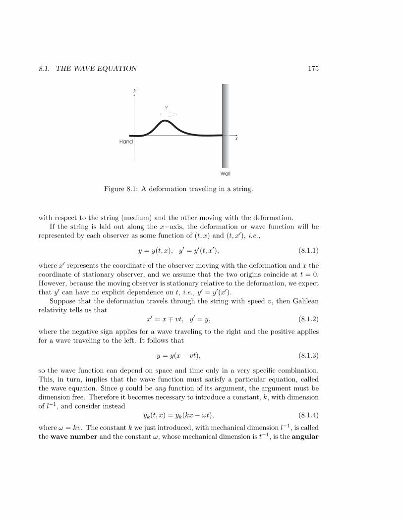
8.1. THE WAVE EQUATION 175
y
x
v
Wall
Hand
Figure 8.1: A deformation traveling in a string.
with respect to the string (medium) and the other moving with the deformation.If the string is laid out along the x−axis, the deformation or wave function will be
represented by each observer as some function of (t, x) and (t, x′), i.e.,
y = y(t, x), y′ = y′(t, x′), (8.1.1)
where x′ represents the coordinate of the observer moving with the deformation and x thecoordinate of stationary observer, and we assume that the two origins coincide at t = 0.However, because the moving observer is stationary relative to the deformation, we expectthat y′ can have no explicit dependence on t, i.e., y′ = y′(x′).
Suppose that the deformation travels through the string with speed v, then Galileanrelativity tells us that
x′ = x∓ vt, y′ = y, (8.1.2)
where the negative sign applies for a wave traveling to the right and the positive appliesfor a wave traveling to the left. It follows that
y = y(x− vt), (8.1.3)
so the wave function can depend on space and time only in a very specific combination.This, in turn, implies that the wave function must satisfy a particular equation, calledthe wave equation. Since y could be any function of its argument, the argument must bedimension free. Therefore it becomes necessary to introduce a constant, k, with dimensionof l−1, and consider instead
yk(t, x) = yk(kx− ωt), (8.1.4)
where ω = kv. The constant k we just introduced, with mechanical dimension l−1, is calledthe wave number and the constant ω, whose mechanical dimension is t−1, is the angular
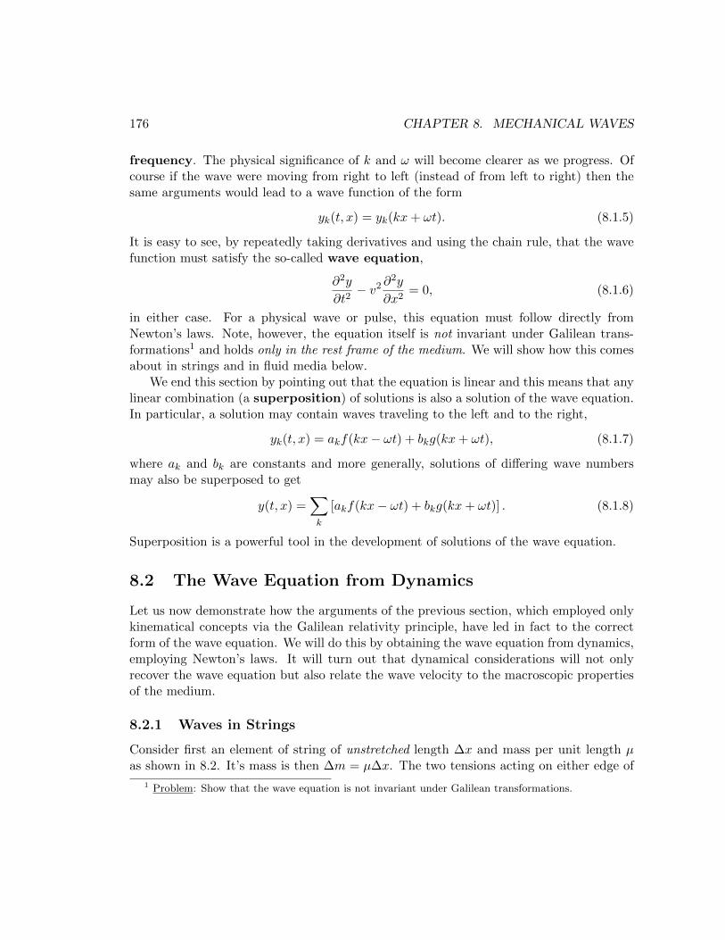
176 CHAPTER 8. MECHANICAL WAVES
frequency. The physical significance of k and ω will become clearer as we progress. Ofcourse if the wave were moving from right to left (instead of from left to right) then thesame arguments would lead to a wave function of the form
yk(t, x) = yk(kx+ ωt). (8.1.5)
It is easy to see, by repeatedly taking derivatives and using the chain rule, that the wavefunction must satisfy the so-called wave equation,
∂2y
∂t2− v2 ∂
2y
∂x2= 0, (8.1.6)
in either case. For a physical wave or pulse, this equation must follow directly fromNewton’s laws. Note, however, the equation itself is not invariant under Galilean trans-formations1 and holds only in the rest frame of the medium. We will show how this comesabout in strings and in fluid media below.
We end this section by pointing out that the equation is linear and this means that anylinear combination (a superposition) of solutions is also a solution of the wave equation.In particular, a solution may contain waves traveling to the left and to the right,
yk(t, x) = akf(kx− ωt) + bkg(kx+ ωt), (8.1.7)
where ak and bk are constants and more generally, solutions of differing wave numbersmay also be superposed to get
y(t, x) =∑k
[akf(kx− ωt) + bkg(kx+ ωt)] . (8.1.8)
Superposition is a powerful tool in the development of solutions of the wave equation.
8.2 The Wave Equation from Dynamics
Let us now demonstrate how the arguments of the previous section, which employed onlykinematical concepts via the Galilean relativity principle, have led in fact to the correctform of the wave equation. We will do this by obtaining the wave equation from dynamics,employing Newton’s laws. It will turn out that dynamical considerations will not onlyrecover the wave equation but also relate the wave velocity to the macroscopic propertiesof the medium.
8.2.1 Waves in Strings
Consider first an element of string of unstretched length ∆x and mass per unit length µas shown in 8.2. It’s mass is then ∆m = µ∆x. The two tensions acting on either edge of
1 Problem: Show that the wave equation is not invariant under Galilean transformations.
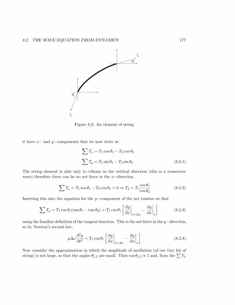
8.2. THE WAVE EQUATION FROM DYNAMICS 177
Figure 8.2: An element of string
it have x− and y−components that we now write as∑Tx = T1 cos θ1 − T2 cos θ2∑Ty = T1 sin θ1 − T2 sin θ2 (8.2.1)
The string element is able only to vibrate in the vertical direction (this is a transversewave) therefore there can be no net force in the x−direction,∑
Tx = T1 cos θ1 − T2 cos θ2 = 0⇒ T2 = T1cos θ1
cos θ2(8.2.2)
Inserting this into the equation for the y−component of the net tension we find∑Ty = T1 cos θ1(tan θ1 − tan θ2) = T1 cos θ1
[∂y
∂x
∣∣∣∣x+∆x
− ∂y
∂x
∣∣∣∣x
](8.2.3)
using the familiar definition of the tangent function. This is the net force in the y−direction,so by Newton’s second law,
µ∆x∂2y
∂t2= T1 cos θ1
[∂y
∂x
∣∣∣∣x+∆x
− ∂y
∂x
∣∣∣∣x
](8.2.4)
Now consider the approximation in which the amplitude of oscillation (of our tiny bit ofstring) is not large, so that the angles θ1,2 are small. Then cos θ1,2 ≈ 1 and, from the
∑Tx
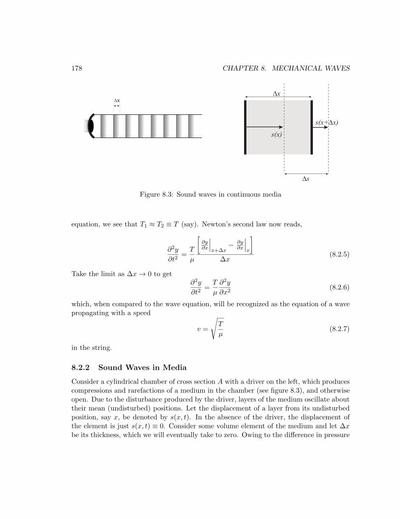
178 CHAPTER 8. MECHANICAL WAVES
Dx
Figure 8.3: Sound waves in continuous media
equation, we see that T1 ≈ T2 ≡ T (say). Newton’s second law now reads,
∂2y
∂t2=T
µ
[∂y∂x
∣∣∣x+∆x
− ∂y∂x
∣∣∣x
]∆x
(8.2.5)
Take the limit as ∆x→ 0 to get∂2y
∂t2=T
µ
∂2y
∂x2(8.2.6)
which, when compared to the wave equation, will be recognized as the equation of a wavepropagating with a speed
v =
√T
µ(8.2.7)
in the string.
8.2.2 Sound Waves in Media
Consider a cylindrical chamber of cross section A with a driver on the left, which producescompressions and rarefactions of a medium in the chamber (see figure 8.3), and otherwiseopen. Due to the disturbance produced by the driver, layers of the medium oscillate abouttheir mean (undisturbed) positions. Let the displacement of a layer from its undisturbedposition, say x, be denoted by s(x, t). In the absence of the driver, the displacement ofthe element is just s(x, t) ≡ 0. Consider some volume element of the medium and let ∆xbe its thickness, which we will eventually take to zero. Owing to the difference in pressure
8.2. THE WAVE EQUATION FROM DYNAMICS 179
on the sides of the element, the net force in the x−direction experienced by this elementis
Fx = [p(x)− p(x+ ∆x)]A (8.2.8)
Since the mass of the element is ∆m = ρA∆x, where ρ is the mass density and A∆x = ∆Vis its volume, we have
ρ∆x∂2s
∂t2= [p(x)− p(x+ ∆x)] ⇒ ρ
∂2s
∂t2= −∂p
∂x(8.2.9)
It’s worth introducing the so-called Bulk Modulus of the medium (a bulk property, whichwill play the role of the tension in the string). It is defined by
B = −V(∂p
∂V
)process
(8.2.10)
where (p, V ) are the pressure and volume of some region. The Bulk modulus of any mediumdepends on the process (that is the reason for the subscript in the above equation) andrepresents the response of the medium to stress by measuring the rate at which pressurechanges relative to volume. Eq. (8.2.10) means that the change in pressure within theelement that has been compressed by ∆V is given in terms of the bulk modulus by
∆p = −B∆V
V(8.2.11)
If s(x) represents the displacement from equilibrium of a fluid layer, originally situated atx, then the change in volume of the element upon stress will be
∆V = A[s(x+ ∆x)− s(x)] (8.2.12)
The pressure change within the element is
∆p = −B[s(x+ ∆x)− s(x)
∆x
](8.2.13)
Taking the limit as ∆x→ 0 gives the change in pressure at any fluid layer in terms of thespatial rate at which the fluid layer is displaced in the direction of the traveling wave:
∆p(x) = −B ∂s∂x
(8.2.14)
The actual pressure at any layer is therefore
p(x) = p0 + ∆p = p0 −B∂s
∂x(8.2.15)
180 CHAPTER 8. MECHANICAL WAVES
where p0 represents the unstressed pressure in the medium. Thus,
∂p
∂x= −B ∂
2s
∂x2. (8.2.16)
But, dividing (8.2.9) by ∆x and taking the limit as ∆x→ 0, we get
ρ∂2s
∂t2= −∂p
∂x(8.2.17)
and therefore,∂2s
∂t2=B
ρ
∂2s
∂x2(8.2.18)
which is the wave equation. Comparison shows that the speed of sound is given by
v =
√B
ρ(8.2.19)
Let’s see how it works for the propagation of sound in an ideal gas.Sound traveling through dry air, for example, is essentially an adiabatic process even
though it may seem that the surrounding air would act as a reservoir. The sound wavecauses oscillations in pressure but the oscillations are fast enough that energy cannot betransferred in the form of heat from compressed regions to rarified regions in such a wayas to keep the temperature constant. For an adiabatic process, the effective equation ofstate is
pV γ = const.⇒(∂p
∂V
)ad
= −γ pV⇒ B = γp (8.2.20)
Using p = nkT = ρkT/m, where m is the average molecular mass,
v =
√γp
ρ=
√γkT
m(8.2.21)
For the (diatomic) “molecule of air” γ = 7/5 and m = 28.8 u. We find v ≈ 347.1 m/s.For an isothermal propagation on the other hand we should have
B = −V(∂p
∂V
)T
= p→ v =
√kT
m(8.2.22)
which is smaller than the result for adiabatic propagation by about 15.5%.Although the wave equation is given in terms of the displacement, s, of layers of the
medium, we can give it in terms of the pressure in the medium. For example, a sinusoidalwave
s(x, t) = smax sin(kx− ωt), (8.2.23)
8.3. ENERGY TRANSFER 181
using (8.2.15), gives
∆p = −Bksmax cos(kx− ωt) (8.2.24)
Substituting B = ρv2 and kv = ω gives
∆p = −ρvωsmax cos(kx− ωt) (8.2.25)
Notice that it is 90 out of phase with the displacement.2 Therefore the maximum valueof the pressure is related to the maximum of the displacement,
∆pmax = ρvωsmax (8.2.26)
as one expects.
8.3 Energy Transfer
8.3.1 Waves in Strings
The energy contained by a unit length of the string is the sum of its kinetic and itspotential energies. For the kinetic energy we could write (per unit length)
dK
dx=
1
2µv2
y =1
2µ
(∂y
∂t
)2
(8.3.1)
For the potential energy, we identify the force on a unit length of the string from the righthand side of the wave equation, i.e.,
F = T∂2y
∂x2. (8.3.2)
This force is directed opposite to the displacement (in the y direction) and so the potentialenergy (per unit length) is
dU
dx= −
∫ y
(−F )dy =
∫ y
T∂2y
∂x2dy = T
∫ y
y′∂y′
∂ydy =
1
2T
(∂y
∂x
)2
(8.3.3)
where y′ = ∂y/∂x. The total energy per unit length of the string is therefore
dE
dx=
1
2µ
[(∂y
∂t
)2
+ v2
(∂y
∂x
)2]
(8.3.4)
2Problem: why does this make sense?
182 CHAPTER 8. MECHANICAL WAVES
where we used T = µv2. The precise value of this energy per unit length would dependon the wave-form y(t, x), but it follows that the energy contained between x1 and x2 canbe given by
E =1
2
∫ x2
x1
dx µ
[(∂y
∂t
)2
+ v2
(∂y
∂x
)2]
(8.3.5)
where y represents the deformation of the string by the wave.
As a simple but useful example consider a right moving, sinusoidal wave given by
y(t, x) = ymax sin(kx− ωt) (8.3.6)
and note that
∂y
∂t= −ωymax cos(kx− ωt), ∂y
∂x= kymax cos(kx− ωt) (8.3.7)
thendE
dx=
1
2µy2
max(ω2 + v2k2) cos2(kx− ωt) (8.3.8)
but, because v = ω/k, we find that the energy contained in a segment from x1 to x2 ofthe string
E = µω2y2max
∫ x2
x1
cos2(kx− ωt)dx (8.3.9)
In particular, over one entire wavelength,
Eλ = µω2y2max
∫ a+λ
acos2
(2πx
λ− ωt
)dx =
1
2µω2y2
maxλ (8.3.10)
where a is any starting point on the string. As the wave propagates, the energy transferredper second is then
P =Eλτ
=1
2µω2y2
max
λ
τ=
1
2µω2y2
maxv (8.3.11)
because τ is the period. Notice that the kinetic and potential energies contribute equallyto the total energy over a wavelength,
Kλ = Uλ =1
4µω2y2
maxλ (8.3.12)
as they do for the simple harmonic oscillator over one period.
8.3. ENERGY TRANSFER 183
8.3.2 Sound Waves
The energy contained by a unit volume of the medium is the sum of its kinetic and itspotential energies. For the kinetic energy we could write (per unit volume)
dK
dV=
1
2ρv2s =
1
2ρ
(∂s
∂t
)2
(8.3.13)
For the potential energy, we identify the force on a unit volume of the medium from theright hand side of the wave equation, i.e.,
F = B∂2s
∂x2. (8.3.14)
This force is directed opposite to the displacement and so the potential energy (per unitvolume) is
dU
dV= −
∫ s
(−F )ds =
∫ s
B∂2s
∂x2ds = B
∫ s
s′∂s′
∂sds =
1
2B
(∂s
∂x
)2
(8.3.15)
where s′ = ∂s/∂x as before. The total energy per unit volume is therefore
dE
dV=
1
2ρ
[(∂s
∂t
)2
+ v2
(∂s
∂x
)2], (8.3.16)
where we used B = ρv2, and gives the energy contained in any volume V of the mediumcontaining the travelling wave
E =1
2
∫VdV ρ
[(∂s
∂t
)2
+ v2
(∂s
∂x
)2]. (8.3.17)
The precise value of this energy per unit length would depend on the wave-form s(x, t).Again consider right-moving sinusoidal waves,
s(x, t) = smax sin(kx− ωt) (8.3.18)
traveling in the positive x−direction, and note that
∂s
∂t= −ωsmax cos(kx− ωt), ∂s
∂x= ksmax cos(kx− ωt) (8.3.19)
thendE
dV=
1
2ρs2
max(ω2 + v2k2) cos2(kx− ωt) (8.3.20)
184 CHAPTER 8. MECHANICAL WAVES
but, because v = ω/k and because we can write dV = Adx, we find that the energycontained in a cylindrical region of cross-sectional area A between x1 to x2 of the mediumis
E = (ρA)ω2s2max
∫ x2
x1
cos2(kx− ωt)dx (8.3.21)
(assuming a constant density). In particular, over one entire wavelength we find
Eλ = (ρA)ω2s2max
∫ a+λ
acos2
(2πx
λ− ωt
)dx =
1
2(ρA)ω2s2
maxλ (8.3.22)
where a is any starting point. As the wave propagates, the energy transferred per secondthrough the medium by the sound way is then
P =Eλτ
=1
2(ρA)ω2s2
max
λ
τ=
1
2(ρA)ω2s2
maxv (8.3.23)
because τ is the period. As before, the kinetic and potential energies contribute equallyto the total energy over an entire wavelength,
Kλ = Uλ =1
4(ρA)ω2s2
maxλ. (8.3.24)
8.4 Solutions of the Wave Equation
A direct and standard approach to solving linear partial differential equations of the aboveform is to apply the method of “separation of variables”. In applying this method oneassumes that the solution is “separable” i.e., that it can be expressed as
y(t, x) = a(t)b(x) (8.4.1)
and therefore it is important to bear in mind that solutions that do not separate as above,if they exist, will not be obtained by this method. Inserting the ansatz into the waveequation gives
d2a(t)
dt2b(x) = v2a(t)
d2b(x)
dx2, or
1
a(t)
d2a(t)
dt2=
v2
b(x)
d2b(x)
dx2(8.4.2)
where, we have divided by a(t)b(x) to obtain the last form. Now the left hand side of theequation depends only on t whereas the right hand side depends only on x. They may beequal to one another only if they are each constant,
1
a(t)
d2a(t)
dt2=
v2
b(x)
d2b(x)
dx2= −ω2. (8.4.3)
8.4. SOLUTIONS OF THE WAVE EQUATION 185
We have called the constant −ω2 so that (i) we may have oscillatory solutions, hence thenegative sign, and (ii) the definition of ω in the previous sections is consistent with oursolutions. Thus we have
d2a(t)
dt2+ ω2a(t) = 0 =
d2b(x)
dx2+ k2b(x) (8.4.4)
where we have made use of the fact that ω = kv. The solutions are therefore
a(t) = Aeiωt +Be−iωt, b(x) = Ceikx +Be−ikx, (8.4.5)
where A,B,C,D are complex coefficients and hence y(t, x) has four terms
y(t, x) = A++ei(kx+ωt) +A+−e
i(kx−ωt) +A−+e−i(kx−ωt) +A−−e
−i(kx+ωt) (8.4.6)
involving eight real degrees of freedom (two per complex coefficient). However, we haveapplied no boundary or initial conditions in obtaining these solutions and such conditionswill greatly reduce the number of degrees of freedom. For example, we already knowthat the solution must be real (since y(t, x) represents some measurable property such asa strng’s displacement or the pressure variations in a fluid) and so the coefficients mustsatisfy the conditions
A++ = A∗−− = A<, A+− = A∗−+ = A> (8.4.7)
where we have used < to indicate left moving waves and > to indicate right movers. Thenumber of degrees of real freedom have thus been reduced to four and y(t, x) can be writtenas
y(t, x) = 2<[A<e
i(kx+ωt) +A>ei(kx−ωt)
](8.4.8)
where < stands for “the real part of”. In all our subsequent analysis we will stick withthe complex expression as far as possible and take the real part only when it is absolutelynecessary. This will simplify the algebra considerably, while not affecting the final resultin any way.
Notice that the phase of the left moving piece is φ< = kx + ωt and that of the rightmoving piece is φ> = kx−ωt. The phases are constant when x = ∓ω
k t = ∓vt respectively.Thus ∓v is called the phase velocity of the plane waves. It is the velocity with whichplane wave fronts travel in space. Holding t fixed (imagine taking a photograph of thewave), we notice that the wave function repeats itself spatially every λ units, where
kλ = 2nπ (8.4.9)
for integer n. The wave number is therefore related to the wavelength, λ, according tok = 2π/λ. On the other hand, viewing the same spatial point (i.e., holding x fixed) thewave function is seen to repeat itself in a time τ , which satisfies
ωτ = 2nπ (8.4.10)
186 CHAPTER 8. MECHANICAL WAVES
for integer n and so the angular frequency is related to the period, τ , according to ω =2π/τ . The frequency of the wave is related to the angular frequency by f = 1/τ = ω/2π.
8.5 Boundary Conditions and Particular Solutions
We must now consider what boundary conditions are to be satisfied by the wave. Boundaryconditions are crucial as they are what determine the actual wave forms encountered in anygiven physical situation. As examples, we will consider two common types of particularsolutions below.
8.5.1 Standing Waves
A “standing wave” is a solution of the wave equation that is required to possess cer-tain characteristics at the boundary. In the case of (one dimensional) waves in string,the boundary would correspond two distinct points on the string; in the case of (one di-mensional) sound waves, the boundary would correspond to two two-dimensional surfacesperpendicular the direction of propagation. At each boundary we may require either (i)that the wave function vanishes there or (ii) that the wave function achieves a maximumthere. Thus three possibilities occur: (a) the wave vanishes at both boundaries (b) itvanishes at one boundary but is maximum at the other and (c) it is maximum at bothboundaries. Standing waves are formed by musical instruments. Every string instrument,for example produces a standing wave in accordance with boundary condition (a) becausethe strings are held fixed at two ends. On the other hand, wind instruments may bedesigned to obey the boundary conditions of types (b) or (c). For instance, a clarinethas one closed end, where the sound waves are required to vanish, and therefore obeyscondition (b) whereas flutes and oboes have both ends open and the sound waves achievetheir maximum value at both ends, so they obey condition (c).
We will begin with cases (a) and (b). For convenience, choose the point at which thewave vanishes as the origin of coordinates and the other at a distance L from it, then thecondition
y(t, 0) = A<eiωt +A∗<e
−iωt +A>e−iωt +A∗>e
iωt = 0 (8.5.1)
implies that
A< = −A∗> (8.5.2)
and inserting this into the wave equation gives
y(t, x) = 2<[A<e
i(kx+ωt) −A∗<ei(kx−ωt)]
(8.5.3)
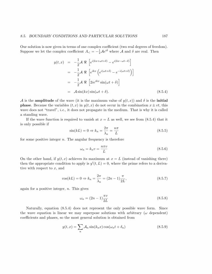
8.5. BOUNDARY CONDITIONS AND PARTICULAR SOLUTIONS 187
Our solution is now given in terms of one complex coefficient (two real degrees of freedom).Suppose we let the complex coefficient A< = −1
4Aeiδ where A and δ are real. Then
y(t, x) = −1
2A <
[ei(kx+ωt+δ) − ei(kx−ωt−δ)
]= −1
2A <
[eikx
(ei(ωt+δ) − e−i(ωt+δ)
)]= −1
2A <
[2ieikx sin(ωt+ δ)
]= A sin(kx) sin(ωt+ δ). (8.5.4)
A is the amplitude of the wave (it is the maximum value of y(t, x)) and δ is the initialphase. Because the variables (t, x) in y(t, x) do not occur in the combination x± vt, thiswave does not “travel”, i.e., it does not propagate in the medium. That is why it is calleda standing wave.
If the wave function is required to vanish at x = L as well, we see from (8.5.4) that itis only possible if
sin(kL) = 0⇒ kn =2π
λn=nπ
L(8.5.5)
for some positive integer n. The angular frequency is therefore
ωn = knv =nπv
L(8.5.6)
On the other hand, if y(t, x) achieves its maximum at x = L (instead of vanishing there)then the appropriate condition to apply is y′(t, L) = 0, where the prime refers to a deriva-tive with respect to x, and
cos(kL) = 0⇒ kn =2π
λn= (2n− 1)
π
2L, (8.5.7)
again for a positive integer, n. This gives
ωn = (2n− 1)πv
2L(8.5.8)
Naturally, equation (8.5.4) does not represent the only possible wave form. Sincethe wave equation is linear we may superpose solutions with arbitrary (ω dependent)coefficients and phases, so the most general solution is obtained from
y(t, x) =∑n
An sin(knx) cos(ωnt+ δn) (8.5.9)
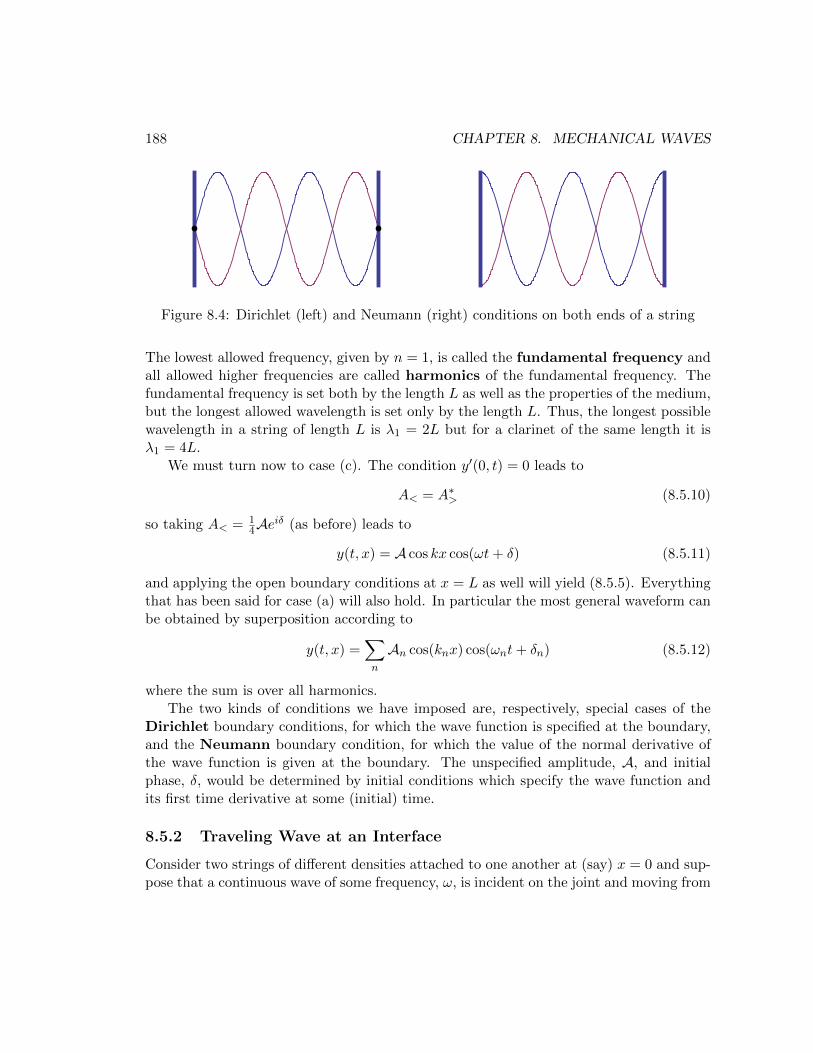
188 CHAPTER 8. MECHANICAL WAVES
Figure 8.4: Dirichlet (left) and Neumann (right) conditions on both ends of a string
The lowest allowed frequency, given by n = 1, is called the fundamental frequency andall allowed higher frequencies are called harmonics of the fundamental frequency. Thefundamental frequency is set both by the length L as well as the properties of the medium,but the longest allowed wavelength is set only by the length L. Thus, the longest possiblewavelength in a string of length L is λ1 = 2L but for a clarinet of the same length it isλ1 = 4L.
We must turn now to case (c). The condition y′(0, t) = 0 leads to
A< = A∗> (8.5.10)
so taking A< = 14Ae
iδ (as before) leads to
y(t, x) = A cos kx cos(ωt+ δ) (8.5.11)
and applying the open boundary conditions at x = L as well will yield (8.5.5). Everythingthat has been said for case (a) will also hold. In particular the most general waveform canbe obtained by superposition according to
y(t, x) =∑n
An cos(knx) cos(ωnt+ δn) (8.5.12)
where the sum is over all harmonics.The two kinds of conditions we have imposed are, respectively, special cases of the
Dirichlet boundary conditions, for which the wave function is specified at the boundary,and the Neumann boundary condition, for which the value of the normal derivative ofthe wave function is given at the boundary. The unspecified amplitude, A, and initialphase, δ, would be determined by initial conditions which specify the wave function andits first time derivative at some (initial) time.
8.5.2 Traveling Wave at an Interface
Consider two strings of different densities attached to one another at (say) x = 0 and sup-pose that a continuous wave of some frequency, ω, is incident on the joint and moving from
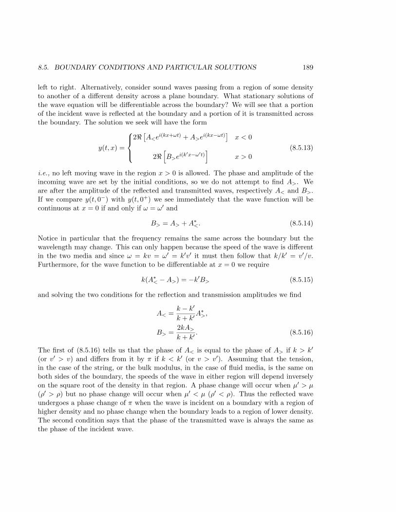
8.5. BOUNDARY CONDITIONS AND PARTICULAR SOLUTIONS 189
left to right. Alternatively, consider sound waves passing from a region of some densityto another of a different density across a plane boundary. What stationary solutions ofthe wave equation will be differentiable across the boundary? We will see that a portionof the incident wave is reflected at the boundary and a portion of it is transmitted acrossthe boundary. The solution we seek will have the form
y(t, x) =
2<[A<e
i(kx+ωt) +A>ei(kx−ωt)] x < 0
2<[B>e
i(k′x−ω′t)]
x > 0
(8.5.13)
i.e., no left moving wave in the region x > 0 is allowed. The phase and amplitude of theincoming wave are set by the initial conditions, so we do not attempt to find A>. Weare after the amplitude of the reflected and transmitted waves, respectively A< and B>.If we compare y(t, 0−) with y(t, 0+) we see immediately that the wave function will becontinuous at x = 0 if and only if ω = ω′ and
B> = A> +A∗<. (8.5.14)
Notice in particular that the frequency remains the same across the boundary but thewavelength may change. This can only happen because the speed of the wave is differentin the two media and since ω = kv = ω′ = k′v′ it must then follow that k/k′ = v′/v.Furthermore, for the wave function to be differentiable at x = 0 we require
k(A∗< −A>) = −k′B> (8.5.15)
and solving the two conditions for the reflection and transmission amplitudes we find
A< =k − k′
k + k′A∗>,
B> =2kA>k + k′
. (8.5.16)
The first of (8.5.16) tells us that the phase of A< is equal to the phase of A> if k > k′
(or v′ > v) and differs from it by π if k < k′ (or v > v′). Assuming that the tension,in the case of the string, or the bulk modulus, in the case of fluid media, is the same onboth sides of the boundary, the speeds of the wave in either region will depend inverselyon the square root of the density in that region. A phase change will occur when µ′ > µ(ρ′ > ρ) but no phase change will occur when µ′ < µ (ρ′ < ρ). Thus the reflected waveundergoes a phase change of π when the wave is incident on a boundary with a region ofhigher density and no phase change when the boundary leads to a region of lower density.The second condition says that the phase of the transmitted wave is always the same asthe phase of the incident wave.
190 CHAPTER 8. MECHANICAL WAVES
In our simple example of a sinusoidal wave traveling from left to right, we saw thatthe energy transferred across the string per second is proportional to µω2vy2
max. Thusthe ratio of the power transferred by the reflected wave and the incident wave in the leftportion of the string will be
Pref
Pinc=
∣∣∣∣A<A>∣∣∣∣2 =
(k − k′
k + k′
)2
= R, (8.5.17)
where we replaced ymax by the amplitudes for the incident and reflected waves respectively.R is called the reflection coefficient. Likewise, the ratio of the power transmitted by theoutgoing wave in the right portion of the string to the incident wave (in the left) is
Ptr
Pinc=µ′v′
µv
∣∣∣∣B>A>∣∣∣∣2 (8.5.18)
since ω = ω′. Again, because the string tension in both regions must be the same,
µv2 = µ′v′2 ⇒ µ′v′
µv=v
v′=k′
k, (8.5.19)
where we used v = ω/k and the fact that ω = ω′ in the last step above. Therefore,
Ptr
Pinc=
√µ′
µ
4k2
(k + k′)2=k′
k
4k2
(k + k′)2=
4kk′
(k + k′)2= T, (8.5.20)
and T is called the transmission coefficient. Note that
R+ T = 1, (8.5.21)
which simply restates the law of conservation of energy.
8.6 The Doppler Effect
The Doppler effect consists of the change in the measured frequency of a source, wheneverthe source or the observer or both the source and the observer are moving with respect tothe medium in which the wave travels. Recall that the wave equation is not invariant underGalilean transformations, having the form (8.1.6) only in the rest frame of the medium.The medium’s rest frame thus becomes a canonical reference frame, with respect to whichall quantities must be measured.
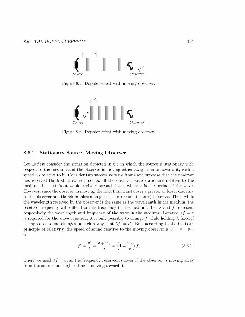
8.6. THE DOPPLER EFFECT 191
l
Source
vObserver
Figure 8.5: Doppler effect with moving observer.
l’
vSource Observer
Figure 8.6: Doppler effect with moving observer.
8.6.1 Stationary Source, Moving Observer
Let us first consider the situation depicted in 8.5 in which the source is stationary withrespect to the medium and the observer is moving either away from or toward it, with aspeed vO relative to it. Consider two successive wave fronts and suppose that the observerhas received the first at some time, t0. If the observer were stationary relative to themedium the next front would arrive τ seconds later, where τ is the period of the wave.However, since the observer is moving, the next front must cover a greater or lesser distanceto the observer and therefore takes a longer or shorter time (than τ) to arrive. Thus, whilethe wavelength received by the observer is the same as the wavelength in the medium, thereceived frequency will differ from its frequency in the medium. Let λ and f representrespectively the wavelength and frequency of the wave in the medium. Because λf = vis required for the wave equation, it is only possible to change f while holding λ fixed ifthe speed of sound changes in such a way that λf ′ = v′. But, according to the Galileanprinciple of relativity, the speed of sound relative to the moving observer is v′ = v ∓ vO,so
f ′ =v′
λ=v ∓ vOλ
=(
1∓ vOv
)f, (8.6.1)
where we used λf = v, so the frequency received is lower if the observer is moving awayfrom the source and higher if he is moving toward it.
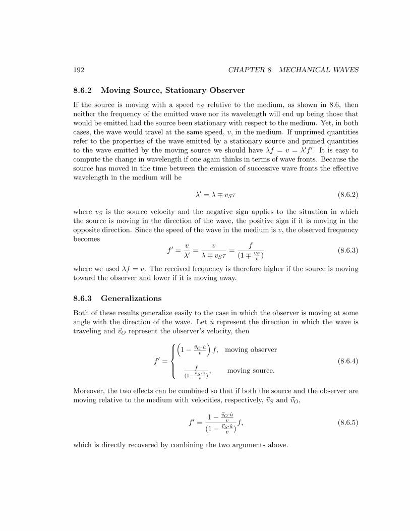
192 CHAPTER 8. MECHANICAL WAVES
8.6.2 Moving Source, Stationary Observer
If the source is moving with a speed vS relative to the medium, as shown in 8.6, thenneither the frequency of the emitted wave nor its wavelength will end up being those thatwould be emitted had the source been stationary with respect to the medium. Yet, in bothcases, the wave would travel at the same speed, v, in the medium. If unprimed quantitiesrefer to the properties of the wave emitted by a stationary source and primed quantitiesto the wave emitted by the moving source we should have λf = v = λ′f ′. It is easy tocompute the change in wavelength if one again thinks in terms of wave fronts. Because thesource has moved in the time between the emission of successive wave fronts the effectivewavelength in the medium will be
λ′ = λ∓ vSτ (8.6.2)
where vS is the source velocity and the negative sign applies to the situation in whichthe source is moving in the direction of the wave, the positive sign if it is moving in theopposite direction. Since the speed of the wave in the medium is v, the observed frequencybecomes
f ′ =v
λ′=
v
λ∓ vSτ=
f
(1∓ vSv )
(8.6.3)
where we used λf = v. The received frequency is therefore higher if the source is movingtoward the observer and lower if it is moving away.
8.6.3 Generalizations
Both of these results generalize easily to the case in which the observer is moving at someangle with the direction of the wave. Let u represent the direction in which the wave istraveling and ~vO represent the observer’s velocity, then
f ′ =
(
1− ~vO·uv
)f, moving observer
f
(1−~vS ·uv
), moving source.
(8.6.4)
Moreover, the two effects can be combined so that if both the source and the observer aremoving relative to the medium with velocities, respectively, ~vS and ~vO,
f ′ =1− ~vO·u
v
(1− ~vS ·uv )
f, (8.6.5)
which is directly recovered by combining the two arguments above.
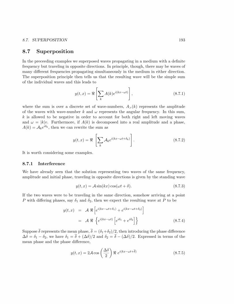
8.7. SUPERPOSITION 193
8.7 Superposition
In the preceeding examples we superposed waves propagating in a medium with a definitefrequency but traveling in opposite directions. In principle, though, there may be waves ofmany different frequencies propagating simultaneously in the medium in either direction.The superposition principle then tells us that the resulting wave will be the simple sumof the individual waves and this leads to
y(t, x) = <
[∑k
A(k)ei(kx−ωt)
], (8.7.1)
where the sum is over a discrete set of wave-numbers, A>(k) represents the amplitudeof the waves with wave-number k and ω represents the angular frequency. In this sum,k is allowed to be negative in order to account for both right and left moving wavesand ω = |k|v. Furthermore, if A(k) is decomposed into a real amplitude and a phase,A(k) = Akeiδk , then we can rewrite the sum as
y(t, x) = <
[∑k
Akei(kx−ωt+δk)
]. (8.7.2)
It is worth considering some examples.
8.7.1 Interference
We have already seen that the solution representing two waves of the same frequency,amplitude and initial phase, traveling in opposite directions is given by the standing wave
y(t, x) = A sin(kx) cos(ωt+ δ). (8.7.3)
If the two waves were to be traveling in the same direction, somehow arriving at a pointP with differing phases, say δ1 and δ2, then we expect the resulting wave at P to be
y(t, x) = A <[ei(kx−ωt+δ1) + ei(kx−ωt+δ2)
]= A <
ei(kx−ωt)
[eiδ1 + eiδ2
](8.7.4)
Suppose δ represents the mean phase, δ = (δ1+δ2)/2, then introducing the phase difference∆δ = δ1 − δ2, we have δ1 = δ + (∆δ)/2 and δ2 = δ − (∆δ)/2. Expressed in terms of themean phase and the phase difference,
y(t, x) = 2A cos
(∆δ
2
)< ei(kx−ωt+δ) (8.7.5)
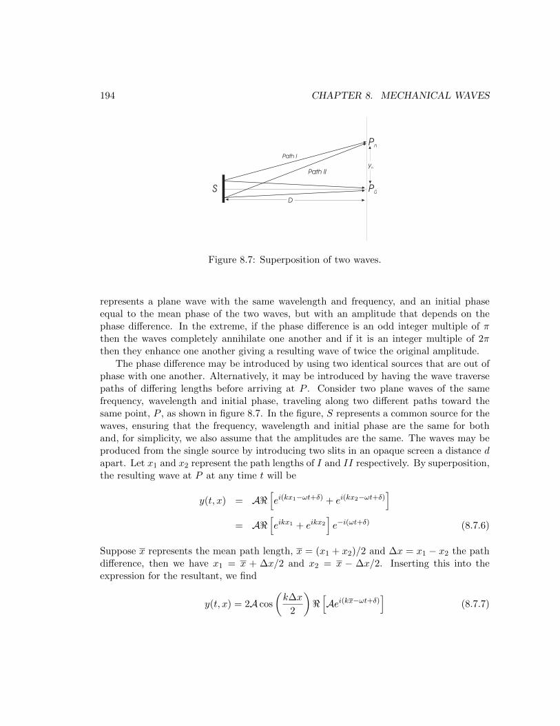
194 CHAPTER 8. MECHANICAL WAVES
Path I
Path II
Pn
P0SD
yn
Figure 8.7: Superposition of two waves.
represents a plane wave with the same wavelength and frequency, and an initial phaseequal to the mean phase of the two waves, but with an amplitude that depends on thephase difference. In the extreme, if the phase difference is an odd integer multiple of πthen the waves completely annihilate one another and if it is an integer multiple of 2πthen they enhance one another giving a resulting wave of twice the original amplitude.
The phase difference may be introduced by using two identical sources that are out ofphase with one another. Alternatively, it may be introduced by having the wave traversepaths of differing lengths before arriving at P . Consider two plane waves of the samefrequency, wavelength and initial phase, traveling along two different paths toward thesame point, P , as shown in figure 8.7. In the figure, S represents a common source for thewaves, ensuring that the frequency, wavelength and initial phase are the same for bothand, for simplicity, we also assume that the amplitudes are the same. The waves may beproduced from the single source by introducing two slits in an opaque screen a distance dapart. Let x1 and x2 represent the path lengths of I and II respectively. By superposition,the resulting wave at P at any time t will be
y(t, x) = A<[ei(kx1−ωt+δ) + ei(kx2−ωt+δ)
]= A<
[eikx1 + eikx2
]e−i(ωt+δ) (8.7.6)
Suppose x represents the mean path length, x = (x1 + x2)/2 and ∆x = x1 − x2 the pathdifference, then we have x1 = x + ∆x/2 and x2 = x − ∆x/2. Inserting this into theexpression for the resultant, we find
y(t, x) = 2A cos
(k∆x
2
)<[Aei(kx−ωt+δ)
](8.7.7)
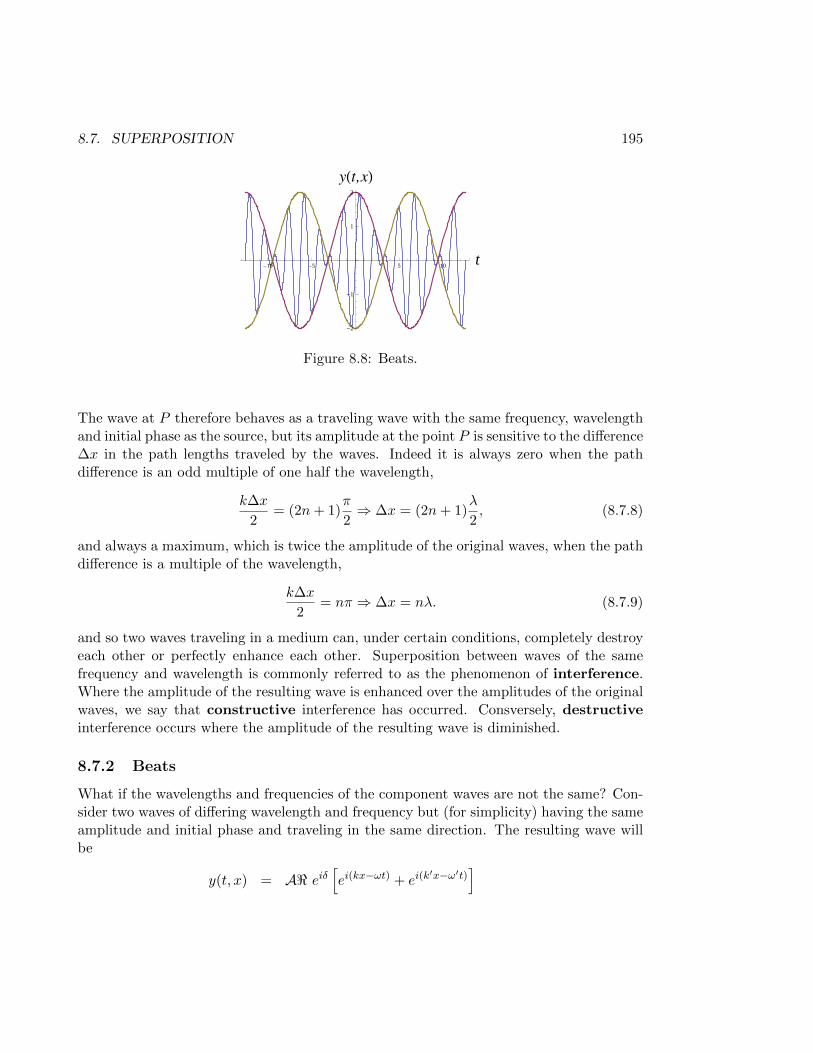
8.7. SUPERPOSITION 195
-10 -5 5 10 t
-2
-1
1
2
yHt,xL
Figure 8.8: Beats.
The wave at P therefore behaves as a traveling wave with the same frequency, wavelengthand initial phase as the source, but its amplitude at the point P is sensitive to the difference∆x in the path lengths traveled by the waves. Indeed it is always zero when the pathdifference is an odd multiple of one half the wavelength,
k∆x
2= (2n+ 1)
π
2⇒ ∆x = (2n+ 1)
λ
2, (8.7.8)
and always a maximum, which is twice the amplitude of the original waves, when the pathdifference is a multiple of the wavelength,
k∆x
2= nπ ⇒ ∆x = nλ. (8.7.9)
and so two waves traveling in a medium can, under certain conditions, completely destroyeach other or perfectly enhance each other. Superposition between waves of the samefrequency and wavelength is commonly referred to as the phenomenon of interference.Where the amplitude of the resulting wave is enhanced over the amplitudes of the originalwaves, we say that constructive interference has occurred. Consversely, destructiveinterference occurs where the amplitude of the resulting wave is diminished.
8.7.2 Beats
What if the wavelengths and frequencies of the component waves are not the same? Con-sider two waves of differing wavelength and frequency but (for simplicity) having the sameamplitude and initial phase and traveling in the same direction. The resulting wave willbe
y(t, x) = A< eiδ[ei(kx−ωt) + ei(k
′x−ω′t)]
196 CHAPTER 8. MECHANICAL WAVES
= 2A cos
[∆k
2x− ∆ω
2t
]< ei(kx−ωt+δ) (8.7.10)
where, as before, we have introduced k = 12(k + k′), ∆k = k − k′ and likewise for ω. The
resultant is therefore made up of two traveling waves: One wave travels with the averagewavelength and frequency of the component waves (this is the frequency perceived by thelistener) and the other is a cosine wave which oscillates with a (lower) frequency, 1
2∆ω, andmodulates the amplitude of the first. The modulation wave is called the beat. Becauseboth waves are traveling in the same medium we know that ω/k = v = ω′/k′, where v isthe speed of the wave in that medium. Therefore the beat or group velocity, which maybe defined as the rate at which a constant amplitude travels through space, is vg = ∆ω/∆kand will be the same as the wave velocity. The frequency of intensity fluctuation will be∆ω/4π. This is called the beat frequency, which, in this particular case, ends up beinghalf the difference in the frequencies of the component waves.
In all the cases analyzed above, we only considered waves traveling with the samevelocity. Our reasoning was that the properties of the medium determine the velocity of atraveling wave and we tacitly assumed that the properties of the medium are insensitiveto the wavelength and frequency of the traveling wave, making the velocity of propagationthe same for all frequencies. There is, however, no fundamental principle that ensures thisto be the case and in fact a more detailed analysis shows that it is only an approximation.Materials in which the velocity of wave propagation is the same for all wavelengths arecalled non-dispersive. Most materials are dispersive, i.e., they will cause waves ofdiffering wavelengths to travel at different speeds. If we account for this dependence of von k then the frequency ω(k) = v(k)k will no longer be linearly related to k and then
vg(k) =∆ω
∆k6= ω
k= v(k). (8.7.11)
In other words, the beat velocity will differ from the phase velocity. The two are related;assuming that ∆k and ∆ω are small, v(k) ≈ v(k) = ω(k)/k and
vg(k) =dω(k)
dk= v(k) + k
dv(k)
dk(8.7.12)
It can be shown that energy and momentum is transferred through the medium with thegroup velocity and therefore it is the group velocity that we measure.
Examples of dispersion in materials abound. For example, the polarizability of amedium changes rapidly when the photon energies approach the energies of quantumtransitions (because of the possibility of resonant absorption), which affects the dielectricconstant and hence the refractive index in a frequency dependent way. Dispersion in theionosphere as the frequency of the radio waves approaches the plasma frequency, is the
8.7. SUPERPOSITION 197
reason why AM radio is accessible at great distances. The changing refractive index ofthe ionosphere leads to “total internal reflection” so that the waves are reflected back toearth.
8.7.3 Wave Packets
If the wave-numbers are allowed to vary continuously, instead of discretely, then the su-perposition sum in (8.7.2) should be replaced by an integral over k,
y(t, x) = <∫ ∞−∞
dkA(k)ei(kx−ω(k)t+δk). (8.7.13)
where the amplitudes must now be understood to carry the appropriate dimensional infor-mation, since A(k)dk represents the amplitude of waves with wavenumber lying betweenk and k + dk. A(k) is the Fourier transform of the wave function and is known as thespectral distribution. A single wave, propagating with wavenumber k0 and amplitudeA0, for example, can be recovered if the spectral distribution is A = A0δ(k−k0). We haveaccounted for dispersion in (8.7.13) by allowing ω(k) to be a general function of k. If thespectral distribution is not a delta function then y(t, x) is called a wave packet.
While plane waves are of infinite extent, wave packets can be “localized” if the spectraldistribution is peaked around some value, say k0, and vanishes rapidly about the peak.Suppose that the integral receives a significant contribution only in a finite interval [k0 −∆k, k0 + ∆k] about k0. Then
y(t, x) ≈ < ei(k0x−ω(k0)t)
∫ ∆k
−∆kdkA(k0) +A′′(k0)k2eik(x−ω′(k0)t)+iδk , (8.7.14)
where k = k− k0. The term we have been able to take out of the integral is a plane wave,propagating at the phase velocity v = ω(k0)/k0. The integral term should be viewed asthe beat since the condition k < ∆k k0 ensures that the exponential outside the integraloscillates rapidly compared with the exponential inside integral. Coherent propagation ofthe amplitude will occur when x− ω′(k0)t = const., i.e., when
dx
dt= ω′(k0) = vg(k0) =
dω(k)
dk
∣∣∣∣k=k0
(8.7.15)
This is the group velocity, as we saw earlier, and it is related to the phase velocity by(8.7.12).
Let us close with the simple example of a “gaussian” wave packet, for which the spectraldistribution is of the form
A(k) = ae−b(k−k0)2 , (8.7.16)
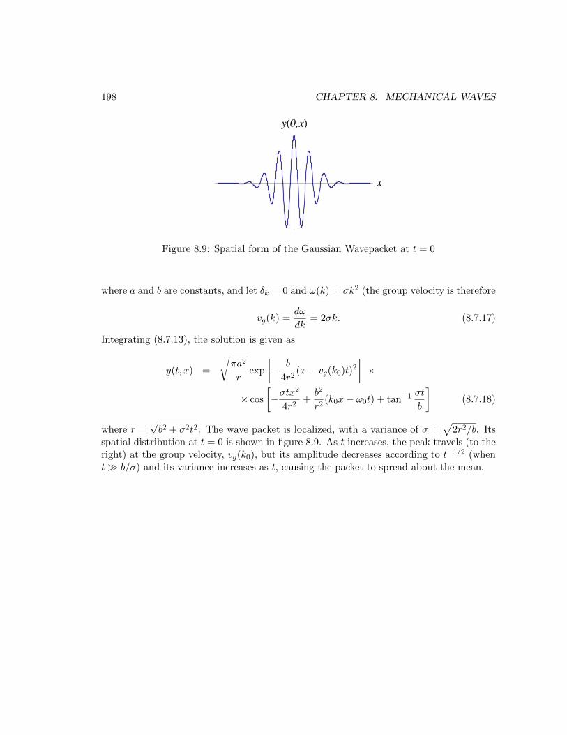
198 CHAPTER 8. MECHANICAL WAVES
x
yH0,xL
Figure 8.9: Spatial form of the Gaussian Wavepacket at t = 0
where a and b are constants, and let δk = 0 and ω(k) = σk2 (the group velocity is therefore
vg(k) =dω
dk= 2σk. (8.7.17)
Integrating (8.7.13), the solution is given as
y(t, x) =
√πa2
rexp
[− b
4r2(x− vg(k0)t)2
]×
× cos
[−σtx
2
4r2+b2
r2(k0x− ω0t) + tan−1 σt
b
](8.7.18)
where r =√b2 + σ2t2. The wave packet is localized, with a variance of σ =
√2r2/b. Its
spatial distribution at t = 0 is shown in figure 8.9. As t increases, the peak travels (to theright) at the group velocity, vg(k0), but its amplitude decreases according to t−1/2 (whent b/σ) and its variance increases as t, causing the packet to spread about the mean.
Chapter 9
The Calculus of Variations
We are now going to embark on a different approach to mechanics than the one we havetaken so far. The new approach involves looking for some quantity that appears to beoptimized by the physical system. Once the quantity is discovered, the mathematicaltechniques that we introduce in this chapter allow us to compute the equations of motionof the system. It should always be remembered that the equations of motion are nodifferent than those that would follow from a careful application of Newton’s laws. Thefundamental principles of mechanics, as embodied in Newton’s three laws do not change,only our way of thinking about them and the techniques used to execute what in the endis Newton’s program are enlarged and made more powerful. Yet, the new approach isnot just about formalism. It also provides a significantly deeper insight into Newton’slaws themselves. It makes manifest the underlying symmetries of the mechanical systemand relates the conservation laws to the symmetries. A famous theorem by the Englishmathematician Emmy Noether showed that the relationship between symmetries of thequantity that is optimized and conservation laws obeyed by the system is a profound one.We will explore Noether’s theorem in considerable depth as we go along.
One of the most significant uses of the new formalism will be the ease with which it ispossible to incorporate constraints: for instance, one may be interested in the motion of abody subject to the action of some known forces but constrained to move only along somesurface. While not impossible to handle, such problems are far from easy if all that wereavailable to us were the methods that have already been introduced. The techniques weare about to learn will significantly simplify them. Because of the relationship they bearwith underlying symmetries and because they are able to handle constrained systems sonaturally, the approach finds its most powerful use in the treatment of field theories.
The new techniques are based upon the “calculus of variations”, which we examinein this chapter. This chapter should be thought of as an essential mathematical detour.From the mathematical point of view, the problem is one of extremization. Only, this time
199
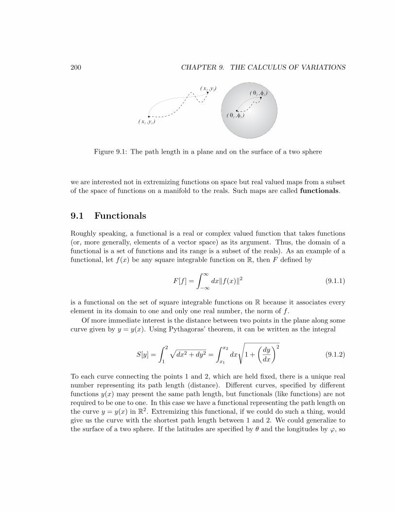
200 CHAPTER 9. THE CALCULUS OF VARIATIONS
( x ,y )1 1
( , )q f1 1
( , )q f2 2
( x ,y )2 2
Figure 9.1: The path length in a plane and on the surface of a two sphere
we are interested not in extremizing functions on space but real valued maps from a subsetof the space of functions on a manifold to the reals. Such maps are called functionals.
9.1 Functionals
Roughly speaking, a functional is a real or complex valued function that takes functions(or, more generally, elements of a vector space) as its argument. Thus, the domain of afunctional is a set of functions and its range is a subset of the reals). As an example of afunctional, let f(x) be any square integrable function on R, then F defined by
F [f ] =
∫ ∞−∞
dx‖f(x)‖2 (9.1.1)
is a functional on the set of square integrable functions on R because it associates everyelement in its domain to one and only one real number, the norm of f .
Of more immediate interest is the distance between two points in the plane along somecurve given by y = y(x). Using Pythagoras’ theorem, it can be written as the integral
S[y] =
∫ 2
1
√dx2 + dy2 =
∫ x2
x1
dx
√1 +
(dy
dx
)2
(9.1.2)
To each curve connecting the points 1 and 2, which are held fixed, there is a unique realnumber representing its path length (distance). Different curves, specified by differentfunctions y(x) may present the same path length, but functionals (like functions) are notrequired to be one to one. In this case we have a functional representing the path length onthe curve y = y(x) in R2. Extremizing this functional, if we could do such a thing, wouldgive us the curve with the shortest path length between 1 and 2. We could generalize tothe surface of a two sphere. If the latitudes are specified by θ and the longitudes by ϕ, so
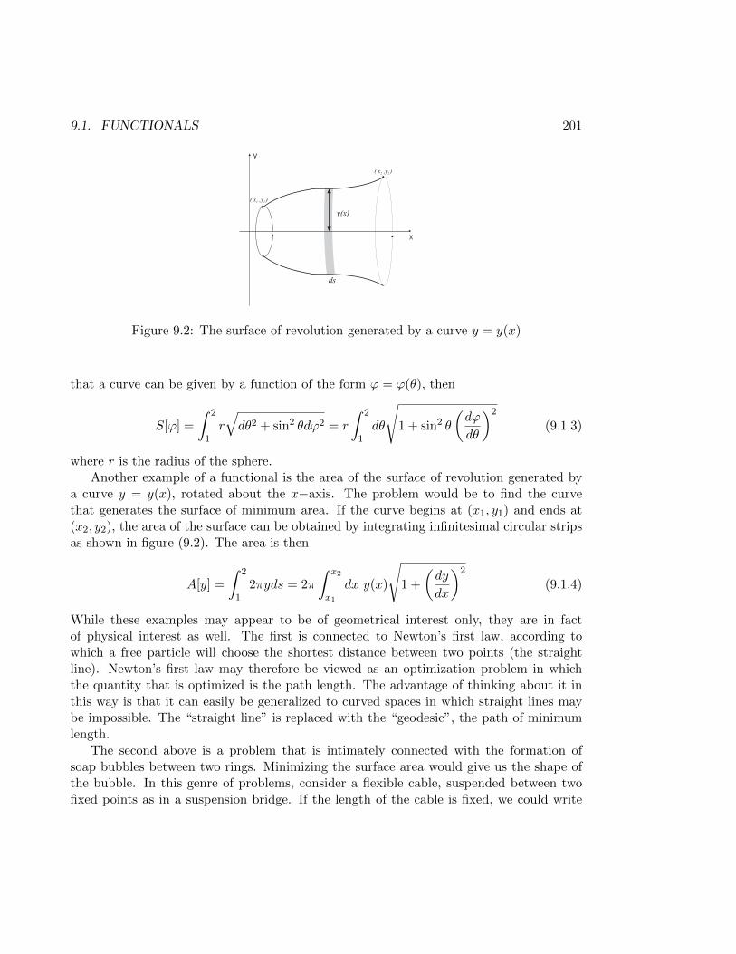
9.1. FUNCTIONALS 201
( x ,y )1 1
( x ,y )2 2
y
x
ds
y(x)
Figure 9.2: The surface of revolution generated by a curve y = y(x)
that a curve can be given by a function of the form ϕ = ϕ(θ), then
S[ϕ] =
∫ 2
1r
√dθ2 + sin2 θdϕ2 = r
∫ 2
1dθ
√1 + sin2 θ
(dϕ
dθ
)2
(9.1.3)
where r is the radius of the sphere.Another example of a functional is the area of the surface of revolution generated by
a curve y = y(x), rotated about the x−axis. The problem would be to find the curvethat generates the surface of minimum area. If the curve begins at (x1, y1) and ends at(x2, y2), the area of the surface can be obtained by integrating infinitesimal circular stripsas shown in figure (9.2). The area is then
A[y] =
∫ 2
12πyds = 2π
∫ x2
x1
dx y(x)
√1 +
(dy
dx
)2
(9.1.4)
While these examples may appear to be of geometrical interest only, they are in factof physical interest as well. The first is connected to Newton’s first law, according towhich a free particle will choose the shortest distance between two points (the straightline). Newton’s first law may therefore be viewed as an optimization problem in whichthe quantity that is optimized is the path length. The advantage of thinking about it inthis way is that it can easily be generalized to curved spaces in which straight lines maybe impossible. The “straight line” is replaced with the “geodesic”, the path of minimumlength.
The second above is a problem that is intimately connected with the formation ofsoap bubbles between two rings. Minimizing the surface area would give us the shape ofthe bubble. In this genre of problems, consider a flexible cable, suspended between twofixed points as in a suspension bridge. If the length of the cable is fixed, we could write
202 CHAPTER 9. THE CALCULUS OF VARIATIONS
an expression for its gravitational potential energy as a sum over the potential energiesinfinitesimal lengths, ds, each located at a height y from some reference level,
U =
∫ 2
1ρgyds = ρg
∫ x2
x1
dx y(x)
√1 +
(dy
dx
)2
(9.1.5)
Minimizing the potential energy would tell us the shape of the cable in equilibrium.
Again, consider a fixed volume of water in a cylindrical container that is rotating witha fixed angular velocity ω. Due to the rotation, the surface of the water will not beplanar but will be such as to minimize the potential energy of the water in the combinedgravitational-centrifugal force field. The potential energy of an infinitesimal volume ofwater of mass δm = ρdV can be written as
δU = δmgy − 1
2δmω2r2 (9.1.6)
since ~Fc = δmω2~r represents the centrifugal force on the element if it is located a distancer from the axis of rotation. Using cylindrical coordinates in which the y axis is the axisof rotations, the total potential energy is
U = ρ
∫ R
0rdr
∫ 2π
0dϕ
∫ y(r)
0dy(gy − 1
2ω2r2) (9.1.7)
where y = y(r) is understood to represent points on the surface of the water. Becauseof axial symmetry, we may perform the ϕ integration right away. Performing also the yintegration gives
U [y] = 2πρ
∫dr r
[gy2(r)− 1
2ω2r2y(r)
](9.1.8)
Minimizing this energy shows that the surface of the water is parabolic.
As a final example, a problem of considerable historical interest is determining thetrajectory of a particle falling in a constant gravitational field in such a way that that thetime taken for it to travel between two points is minimized. We can setup the problem asfollows: the time taken to cover an infinitesimal length of the trajectory is
dt =ds
v(9.1.9)
where v is its instantaneous velocity. Conservation of energy tells us that
1
2mv2
1 +mgy1 =1
2mv2 +mgy (9.1.10)
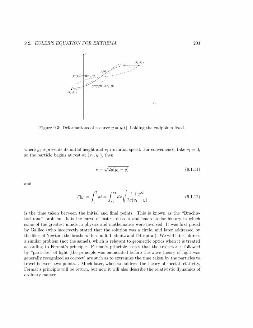
9.2. EULER’S EQUATION FOR EXTREMA 203
(x ,y )1 1
(x ,y )2 2
x
y
y=y (t)+ (t)0 ah 2
y=y (t)+ (t)0 ah 1
y (t)0
Figure 9.3: Deformations of a curve y = y(t), holding the endpoints fixed.
where y1 represents its initial height and v1 its initial speed. For convenience, take v1 = 0,so the particle begins at rest at (x1, y1), then
v =√
2g(y1 − y) (9.1.11)
and
T [y] =
∫ 2
1dt =
∫ x2
x1
dx
√1 + y′2
2g(y1 − y)(9.1.12)
is the time taken between the initial and final points. This is known as the “Brachis-tochrone” problem. It is the curve of fastest descent and has a stellar history in whichsome of the greatest minds in physics and mathematics were involved. It was first posedby Galileo (who incorrectly stated that the solution was a circle, and later addressed bythe likes of Newton, the brothers Bernoulli, Leibnitz and l’Hospital). We will later addressa similar problem (not the same!), which is relevant to geometric optics when it is treatedaccording to Fermat’s principle. Fermat’s principle states that the trajectories followedby “particles” of light (the principle was enunciated before the wave theory of light wasgenerally recognized as correct) are such as to extremize the time taken by the particles totravel between two points. . Much later, when we address the theory of special relativity,Fermat’s principle will be return, but now it will also describe the relativistic dynamics ofordinary matter.
204 CHAPTER 9. THE CALCULUS OF VARIATIONS
9.2 Euler’s equation for extrema
With the motivation provided by the examples in the previous section, we want to obtainthe necessary and sufficient conditions for the existence of an extremum of a functionalwhich has the form
S[y] =
∫ 2
1dtf(y(t), y(t); t) (9.2.1)
We are using t for our independent variable and y(t) as the test function. Suppose thata trajectory that extremizes S[y] exists and call it y0(t). Then consider a one parameterdeformation of the trajectory y0(t) of the form
y(α, t) = y0(t) + αη(t), (9.2.2)
and η(t) is any differentiable function obeying
η(t1) = η(t2) = 0 (9.2.3)
In other words, the the endpoints are held fixed by the deformations, but otherwise theyare arbitrary [see figure (9.3)]. The functional
S[y;α] =
∫ 2
1dtf(y(α, t), y(α, t); t) (9.2.4)
is now also a function of α. The necessary condition for an extremum is
∂S[y;α]
∂α
∣∣∣∣α=0
= 0 (9.2.5)
but we must understand how to take this derivative. Expanding f(y0, y0; t) in a Taylorseries, we have
f(y, y; t) = f(y0, y0; t) + α
[η∂f
∂y
∣∣∣∣α=0
+ η∂f
∂y
∣∣∣∣α=0
]+ . . . (9.2.6)
so that∂S[y;α]
∂α=
∫ 2
1dt
[∂f
∂y
∣∣∣∣α=0
+ η∂f
∂y
∣∣∣∣α=0
]. (9.2.7)
With the understanding that all partial derivatives of f are taken at α = 0, we write thisas
∂S[y;α]
∂α=
∫ 2
1dt
[∂f
∂yη +
∂f
∂yη
]. (9.2.8)
9.2. EULER’S EQUATION FOR EXTREMA 205
The second term can be integrated by parts
∂S[y;α]
∂α
∣∣∣∣α=0
=
∫ 2
1dt
[η∂f
∂y− η d
dt
(∂f
∂y
)]+
[η(t)
∂f
∂y
]2
1
, (9.2.9)
but because the deformations we are considering vanish at the boundaries (η(t1) = 0 =η(t2)), the necessary condition for an extremum becomes
∂S[y;α]
∂α
∣∣∣∣α=0
=
∫ 2
1dt
[∂f
∂y− d
dt
(∂f
∂y
)]η(t) = 0. (9.2.10)
The deformations, η(t), are arbitrary, therefore the integral can vanish only if
∂f
∂y− d
dt
(∂f
∂y
)= 0 (9.2.11)
This necessary condition for the existence of an extremum is known as Euler’s equation.It is equivalent to the usual condition for the existence of an extremum of a simple functionof a single variable in elementary calculus. If the functional S depends on more than oneindependent function, there is one Euler equation for each such independent function.
The left hand side of (9.2.11) is known as the first functional derivative of the S[y]or the Euler derivative of f , and denoted by
δS[y]
δy(t)
def=
∂f
∂y(t)− d
dt
(∂f
∂y(t)
). (9.2.12)
so that a necessary condition for the existence of an extremum is a vanishing first functionalderivative,
δS[y]
δy(t)= 0 (9.2.13)
An alternative (quick and dirty) approach to recovering Euler’s equation that we shall usehenceforth is to consider a “variation” of S under variations of the function y(t) as follows,
δS[y] =
∫ 2
1dt
(∂f
∂yδy +
∂f
∂yδy
)(9.2.14)
where δy = αη. The variations commute with the time derivative of y, i.e.,
δdy
dt=
d
dtδy, i.e.,
[δ,d
dt
]y(t) = 0 (9.2.15)
Integrating by parts (as we did before) and discarding the boundary term because thevariations vanish on the boundary, gives
δS[y] =
∫ 2
1dt
(∂f
∂y− d
dt
∂f
∂y
)δy = 0, (9.2.16)
which imply Euler’s equation by the same argument we used earlier. Let’s apply thisequation to determine the extrema of the functionals we developed earlier.
206 CHAPTER 9. THE CALCULUS OF VARIATIONS
9.3 Examples
9.3.1 Geodesics
Consider first the functional
S[y] =
∫ x2
x1
dx√
1 + y′2 (9.3.1)
which gives the path length between two points on a trajectory specified by y = y(x).Applying Euler’s equation gives a differential equation for the function y(x),
∂f
∂y− d
dx
∂f
∂y′= − d
dx
y′√1 + y′2
= 0 (9.3.2)
which means thaty′√
1 + y′2= c, (9.3.3)
where c is some constant. Solving shows that the solution is of the form y = mx+d, wherem = c/(1− c2) and d is another arbitrary constant. This is the equation of a straight line,as we expected. The two constants (the slope and the y−intercept) are determined by theend points of course. An alternative approach would be to expand the derivative getting[
1√1 + y′2
− y′2
(1 + y′2)3/2
]y′′ =
y′′
(1 + y′2)3/2= 0 (9.3.4)
which is only possible if y′′(x) = 0. This gives the solution y = mx + d. Paths given byfunctions of the form y = y(x) are very special if y(x) is a function because it cannot turninto itself as the function cannot be one to many.
The generalization of this problem to the problem of the geodesic on a sphere can alsobe solved exactly. Our action functional was
S = r
∫ 2
1dθ
√1 + sin2 θϕ′2 (9.3.5)
where the prime now refers to a derivative with respect to ϕ. Euler’s equation is
− d
dθ
(sin2 θϕ′√
1 + sin2 θϕ′2
)= 0 (9.3.6)
which is not dissimilar from the problem of the geodesic in R2. The solution is howeverdifferent. We have
sin2 θϕ′√1 + sin2 θϕ′2
= α (9.3.7)
9.3. EXAMPLES 207
where α is some constant, and simplifying
ϕ′ =α√
sin4 θ − α2 sin2 θ(9.3.8)
or
ϕ =
∫α csc2 θdθ√1− α2 csc2 θ
(9.3.9)
The integral on the right can be solved by the substitution x = α cot θ, which gives
ϕ+ β =
∫dx√
1− α2 − x2= sin−1 x√
1− α2= sin−1
(cot θ
a
)(9.3.10)
where a =√
1− α2/α. The solution is
cot θ = a sin(ϕ+ β) (9.3.11)
To understand what it means, expand the right hand side to rewrite the equation as
cos θ = a(sinϕ cosβ + cosϕ sinβ) sin θ (9.3.12)
and view the sphere as embedded in R3, where
x = r sin θ cosϕ
y = r sin θ sinϕ
z = r cos θ. (9.3.13)
The solution, rewritten in terms of the Cartesian coordinates in the embedding space is
z = Ax+By (9.3.14)
where A and B are constants of the integration, related in an obvious way to a and β. Werecognize this as the equation of a plane passing through the origin, i.e., the center of thesphere! So the geodesic on a sphere is a great circle.1
1Problem: Show that the equation for a geodesic on a cylinder is
ϕ = mz + ϕ0
which is the equation of a helix. By “unwrapping” the cylinder, it turns into a plane. What does thegeodesic look like in the plane?
208 CHAPTER 9. THE CALCULUS OF VARIATIONS
9.3.2 Minimum surface of revolution
Our next problem was to determine the curve whose surface of revolution is minimum.For this we had to extremize the functional
A[y] = 2π
∫ x2
x1
dx y√
1 + y′2. (9.3.15)
The Euler equation for the area functional is
∂f
∂y− d
dx
∂f
∂y′=√
1 + y′2 − d
dx
yy′√1 + y′2
= 0 (9.3.16)
Expand the derivative
√1 + y′2 − yy′′ + y′2√
1 + y′2+
yy′2y′′
(1 + y′2)3/2= 0 (9.3.17)
and simplify to see that this gives the simple equation
(1 + y′2)2 − (1 + y′2)y′2 − yy′′ = 1 + y′2 − yy′′ = 0. (9.3.18)
One may employ the following trick to solve this equation, even though it looks difficult.Divide by (1 + y′2)3/2 and multiply by y′ to write it as
y′√1 + y′2
− yy′y′′
(1 + y′2)3/2=
d
dx
y√1 + y′2
= 0, (9.3.19)
which means thaty√
1 + y′2= c⇒ y′ =
dy
dx= ±
√y2
c2− 1 (9.3.20)
where c is an arbitrary constant. The solution is, of course∫dy√y2
c2− 1
= ±x+ d (9.3.21)
where d is yet another constant of integration. The solution is obtained by the substitutiony = c cosh η
y(x) = c cosh
(x+ d
c
)(9.3.22)
The shape of a cable on a suspension bridge is given by the same solution because thefunctional minimizing the potential energy is the same.

9.3. EXAMPLES 209
9.3.3 The rotating bucket
We have argued that the shape of the surface of water that is rotating in a bucket isdetermined by the functional
U [y] = 2πρ
∫ R
0dr r
[gy2 − 1
2ω2r2y
](9.3.23)
This functional has no derivatives of y(r), so Euler’s equation reads
y(r) =1
4gω2r2 (9.3.24)
which is the equation of a parabola whose steepness is determined by ω2/4g.
9.3.4 The Brachistochrone
We turn finally to the Brachistochrone, which involves minimizing the functional
T [y] =
∫ x2
x1
dx
√1 + y′2
2g(y1 − y). (9.3.25)
and leads to1
2
√1 + y′2
(y1 − y)3/2− d
dx
(y′√
(1 + y′2)(y1 − y)
)= 0 (9.3.26)
Expanding the drivative term,
1
2
√1 + y′2
(y1 − y)3/2− y′′√
(1 + y′2)(y1 − y)+
y′2y′′√y1 − y(1 + y′2)3/2
− y′2
2√
1 + y′2(y1 − y)3/2= 0 (9.3.27)
and simplifying
1
2(1 + y′2)2 − y′′(y1 − y)(1 + y′2) + y′2y′′(y1 − y)− 1
2y′2(1 + y′2) = 0
⇒ 1 + y′2 − 2(y1 − y)y′′ = 0 (9.3.28)
To solve this equation, it’s convenient to eliminate y1 by defining z = y1 − y so that theequation we must solve is
1 + z′2 + 2zz′′ = 0 (9.3.29)
210 CHAPTER 9. THE CALCULUS OF VARIATIONS
and divide by z3/2(1 + z′2)3/2. This gives
1
z3/2√
1 + z′2+
2z′′√z(1 + z′2)3/2
= − d
dx
1√z(1 + z′2)
= 0 (9.3.30)
which, when solved for z′ gives
z′ = ±√c
z− 1⇒
∫ √zdz√c− z
= x+ d (9.3.31)
The solution to this integral is best obtained in parameterized form by making the sub-stitution z = c sin2 θ to rewrite the integral as
2c
∫sin2 θ = x+ d⇒ x =
c
2(2θ − sin 2θ)− d (9.3.32)
Our solution, in parameterized form is therefore
x =c
2(2θ − sin 2θ), y = y1 +
c
2(1− cos 2θ) (9.3.33)
which is a cycloid reflected on the x−axis and vertically shifted by y1 .
9.4 Functional Derivatives
The Euler derivative is also called the first functional derivative of S[y]. It is worthrewriting our definition of this derivative in a way that is more adapted to extending it tohigher order functional derivatives. To this end, define
δS[y] =
∫dtδS[y]
δy(t)η(t) =
∂S[y;α]
∂α
∣∣∣∣α=0
(9.4.1)
and compare the left hand side of the definition to (9.2.10) to see that it is identical to(9.2.12). In this suggestive form, however, it is easy to see how higher functional derivativesare to be defined. A natural extension is
δnS[y] =
∫dt1dt2...dtn
δnS[y]
δy(t1)δy(t2)...δy(tn)η(t1)η(t2)...η(tn)
def=
∂nS[y;α]
∂αn
∣∣∣∣α=0
.
(9.4.2)It turns out that higher order functional derivatives are ultralocal differential operators, i.e.,operators that are proportional to Dirac δ−function(s). The second functional derivativedefines an “eigenvalue” (Sturm-Liouville) problem for η(t) and whether the extrema wehave found are minima or maxima depends on whether or not δ2S[y] > 0, i.e., on the
9.4. FUNCTIONAL DERIVATIVES 211
eigenvalue spectrum of this differential operator. If the spectrum is positive definite theextremum is a minimum.
Let us use the definition in (9.4.2) to determine the second order functional derivativeof (9.2.1). Expanding f(y + αη, y + αy; t) up to second order in α,
f(y, y; t) = f(y0, y0; t) + α
[η∂f
∂y+ η
∂f
∂y
]α=0
+α2
2
[η2∂
2f
∂y2+ ηη
∂2f
∂y∂y+ η2∂
2f
∂y2
]α=0
+ . . .
(9.4.3)so
∂2S[y + αη]
∂α2
∣∣∣∣α=0
=
∫ f
idt
[η2∂
2f
∂y2+ ηη
∂2f
∂y∂y+ η2∂
2f
∂y2
](9.4.4)
Now notice that in the middle term ηη = η2/2 allows us to integrate the second term byparts and drop a total derivative (boundary term) because η is required to vanish there.Therefore
∂2S[y + αη]
∂α2
∣∣∣∣α=0
=
∫ f
idt
[η2
∂2f
∂y2− 1
2
d
dt
(∂2f
∂y∂y
)+ η2∂
2f
∂y2
](9.4.5)
Also integrating the last term once by parts allows us to write the entire expression as
∂2S[y + αη]
∂α2
∣∣∣∣α=0
=
∫ f
idt η
[∂2f
∂y2− 1
2
d
dt
(∂2f
∂y∂y
)− d
dt
(∂2f
∂y2
d
dt
)]η (9.4.6)
and now we’re able to compare it with (9.4.2). Let’s apply this to a simple, but useful typeof functional for which f(y, y; t) = y2/2− v(y). In this case, a straightforward calculationreveals
∂2S[y + αη]
∂α2
∣∣∣∣α=0
= −∫ f
idt η(t)
[∂2v
∂y2+d2
dt2
]η(t) (9.4.7)
or (y1 = y(t1) and y2 = y(t2))
δ2S
δy1δy2= −
[d2
dt21+∂2v(y1)
∂y21
]δ(t1 − t2) (9.4.8)
Consider the eigenvalue equations for this operator,
−[∂2v
∂y2+d2
dt2
]y=y0
φn(t) = λnφn(t), (9.4.9)
where y0(t) represents an extreme value of the functional, i.e. a solution to Euler’s equationand φn(t) represent a complete set of orthonormal eigenfunctions. Let φn(t) be normalizedin the interval [ti, tf ] and vanishing at the boundaries, so that we can set
η(t) =∑n
cnφn(t) (9.4.10)
212 CHAPTER 9. THE CALCULUS OF VARIATIONS
then if we let S[y] = S[y0] + δS[y0] + δ2S[y0] + . . .,
δ2S[y0] =∑n
λnc2n (9.4.11)
To make our example simpler still, take v′′(y) to be ignorable, then our eigenvalue equationbecomes
d2φndt2
+ λnφn = 0 (9.4.12)
Solutions that vanish at the ti and tf can be found. To simplify the algebra, take ti = 0and tf = T , so that the only solutions that vanish at the end points are
φn = A sin√λnt (9.4.13)
where
λn =n2π2
T 2, n ∈ N ∪ 0 (9.4.14)
The eigenvalues are all non-negative, so δ2S[y0] > 0 so, in this case, the extremum of theaction, given by Eulers equations, will represent a minimum. More generally, eg., if v′′(y)were not ignorable, the result would depend on v(y).
9.5 An alternate form of Euler’s equation
There is an alternate form of Euler’s equation, which is particularly useful when f(y, y)does not explicitly depend on t. It can be obtained directly from (9.2.11) by writing
df
dt=∂f
∂t+∂f
∂yy +
∂f
∂yy (9.5.1)
and substitutingd
dt
(∂f
∂yy
)=∂f
∂yy + y
d
dt
(∂f
∂y
)(9.5.2)
we findd
dt
[f − ∂f
∂yy
]=∂f
∂t+
[∂f
∂y− d
dt
(∂f
∂y
)]y. (9.5.3)
But by Euler’s equation, the term in square brackets on right hand side vanishes, therefore
∂f
∂t− d
dt
[f − ∂f
∂yy
]= 0 (9.5.4)
and if f does not depend explicitly on time,
f − ∂f
∂yy = constant (9.5.5)
summarizes the content of (9.2.11). One can immediately see how useful this is as itinvolves just a first order equation.
9.6. FUNCTIONALS INVOLVING SEVERAL FUNCTIONS 213
9.6 Functionals involving several functions
Our considerations so far are easily generalized to functionals of several dependent vari-ables,
S[x1, x2, ...xn] =
∫ 2
1dt f(x1(t), ..., xn(t), x1(t), ..., xn(t), t) (9.6.1)
Such functionals are more adapted to the requirements of mechanics, where even twodimensional trajectories may fold in on themselves and cannot be represented as func-tions, but more generally are not constrained to surfaces. As we know, in mechanics it ismore useful to consider parameterized curves, ~r = ~r(t). We can use the same variationaltechniques as we did before. Once more, requiring
δS =
∫ n∑i=1
(∂f
∂xiδxi +
∂f
∂xiδxi
)= 0 (9.6.2)
gives
δS = 0⇒∫dt
n∑i=1
(∂f
∂xi− d
dt
∂f
∂xi
)δxi = 0 (9.6.3)
which is possible if and only if each term vanishes because the variations δxi(t) are allarbitrary and independent. Therefore we have n Euler equations, one for each dependentvariable,
∂f
∂xi− d
dt
∂f
∂xi= 0, i ∈ 1, ..., n (9.6.4)
which may, or may not be coupled, dependending on the functions f .2
As an example, consider the parameterized curve in R3, given by the three functions,x1(t), x2(t) and x3(t). In this case, the path length can be written as
S =
∫ t2
t1
dt√x2
1 + x22 + x2
3. (9.6.5)
There are therefore three Euler equations, one for each function. We have,
∂f
∂xi− d
dt
∂f
∂xi= − d
dt
xi√x2
1 + x22 + x2
3
= 0 (9.6.6)
2Problem: Show that if f has no explicit dependence on t, then
f −∑i
∂f
∂yiyi = 0
Note that this is just one equation, whereas there are as many Euler’s equations as dependent functions,assuming no external constraints. This is the “alternative” form of the previous section.
214 CHAPTER 9. THE CALCULUS OF VARIATIONS
The vector ~v = (x1, x2, x3) is just the “velocity” and therefore these equations tell us thatv is a constant vector. Since the direction of the velocity vector is constant, the trajectoryis a straight line. We can put the equations in a more suggestive form if we recognize that
ds
dt=√x2
1 + x22 + x2
3 (9.6.7)
and therefore that (9.6.6) can also be written as
dt
ds= 0 (9.6.8)
where t is the unit tangent vector to the curve. In the Serret-Frenet description of curves,this is saying that the curvature is zero. Note that minimizing the path length gives noinformation about the magnitude of the velocity and this means that there are really onlytwo and not three independent equations of motion. One can trace this to “reparametriza-tion invariance”, which means that any transformation t → t′ = f(t), with xi → x′i = xi,leaves the functional S invariant so that the parameter t itself has no physical significance.We will be looking for functionals whose extremization leads to Newton’s laws of motion.However, because Newton’s first law already requires a free body to possess a constantvelocity (therefore both magnitude and direction), this functional is not a good startingpoint.
9.7 Constraints
Often it happens that it is necessary to consider additonal constraints on a system. Forexample, consider the equation of the geodesic on sphere. The way we solved the problemwas to think of the sphere intrinsically i.e., without reference to the three dimensionalspace, R3, in which it is embedded. This is a very useful way to think about curved spaces,but it is not necessary because every such space can also be thought of as embedded in somehigher dimensional space, Rn.3 For example, we could think of the sphere as embeddedin R3. We already know that the shortest distance between two points in R3 is a straightline, but it is far from so on the sphere! To get the shortest distance along the sphere wemust impose an additional condition, a constraint, which explicitly requires that all pointson the trajectory lie on it, i.e., we must also require
x21(t) + x2
2(t) + x23(t) = r2 (9.7.1)
where r is the radius of the sphere.
3Note that the embedding space does not necessarily possess just one dimension more than the embeddedspace.
9.7. CONSTRAINTS 215
In general, when constraints are present, we need to impose additional conditions ofthe form
g(x1, x2, ..., x1, ..., xn) = 0 (9.7.2)
The presence of constraints implies that the variations we make in deriving the Eulerequations are not all independent and therefore δS = 0 does not imply that the Eulerequations hold separately for each dependent variable. Let us first review how constraintsare handled in simple problems not involving functionals.
Consider a cylinder of radius r and length l. How can the surface area be minimizedwhile keeping the volume of the cylinder fixed?. (For example, you may be asked to designa cylindrical container of fixed volume in such a way as to minimize the material used inits construction.) For any r and l, the surface area of the cylinder (including its ends) isA(r, l) = 2πrl + 2πr2 and its volume is V (r, l) = πr2l. In this simple example, we couldsolve the constraint directly,
l =V
πr2(9.7.3)
and rewrite A as a function of r (subject to the constraint)
A(r) =2V
r+ 2πr2 (9.7.4)
Then it is easy to see that r = 3√V/2π gives the radius that minimizes the surface area.
Notice that solving the constraint first reduces the number of independent variables (inthis case, r and l). It also complicates the function to be extremized. Sometimes it maybe difficult to solve the constraint equation(s); what then do we do? We follow a methodintroduced by and named after the mathematician Joseph Louis Lagrange.
To motivate Lagrange’s approach, consider having to extremize a function S of twovariables, xi, i ∈ 1, 2, subject to a constraint of the form g(xi) = 0. The extremizationcondition for S is
δS =∑i
∂S
∂xiδxi = 0 (9.7.5)
but because the variables are not all independent on account of the constraint, we cannotset each first partial derivative to zero independently. Instead, noting that g(xi) = 0, varythe constraint also to get
δg(xi) = 0 =∑i
∂g
∂xiδxi (9.7.6)
Of course, this means that
δx2 = −∂g/∂x1
∂g/∂x2δx1 (9.7.7)
216 CHAPTER 9. THE CALCULUS OF VARIATIONS
Inserting this into the variation of S, we find
δS =
[∂S
∂x1− ∂S
∂x2
∂g/∂x1
∂g/∂x2
]δx1 (9.7.8)
or∂S
∂x1
(∂g
∂x1
)−1
=∂S
∂x2
(∂g
∂x2
)−1
(9.7.9)
However, because the left hand side involves only derivatives with respect to x1 and theright only derivatives with respect to x2, the two must be equal to some constant, −λ. Inparticular,
∂S
∂xi+ λ
∂g
∂xi= 0, i ∈ 1, 2 (9.7.10)
and, if we call S = S + λg, then not only do we have
∂S∂xi
= 0, i ∈ 1, 2 (9.7.11)
but also∂S∂λ
= 0, (9.7.12)
which reproduces the constraint g(xi) = 0. The three equations (9.7.11) and (9.7.12) aresufficient to solve for the three variables xi and λ and constitute a general solution of theextremzation problem when constraints are present. The extra variable that was intro-duced (λ) has come to be called a Lagrange multiplier. The method is easily extended (bymathematical induction) to the case of n variables and any number m < n of constraints.We need one Lagrange multiplier for each constraint.
Lagrange thus turned a problem originally involving n variables satisfying m < nconstraints (our simple example involves two variables and one constraint) into a probleminvolving n+m variables and no constraints by introducing the Lagrange multipliers.In our toy example, instead of considering A(r, l) we consider the function
A = A(r, l) + λ(V (r, l)− V0) (9.7.13)
where λ is a new variable (called a Lagrange multiplier) that multiplies the constraint andV0 is the desired volume of the container. Notice that if all variables are independent,then A is extreme only if its first derivative with respect to each variable vanishes
∂A∂r
= 2π(l + 2r + λrl) = 0
∂A∂l
= 2π
(r +
λ
2r2
)= 0
9.7. CONSTRAINTS 217
∂A∂λ
= πr2l − V0 = 0. (9.7.14)
We have three equations for the three variables r, l, λ. The last equation makes the con-straint explicit. The second equation, when solved for λ gives λ = −2/r and when thisvalue of λ is inserted into the first equation we obtain l = 2r. With this value of l, the lastequation gives precisely r = 3
√V0/2π. The cost of using Lagrange multipliers is that we
have had to solve three equations simultaneously, whereas we would have had to solve justone equation if the constraint were solved at the start and l replaced by an appropriatefunction of r. In general, when there are m < n constraints in the system, the use ofLagrange multipliers introduces an additional 2m equations. The lesson is that if the con-straints can be solved at the start, it is best to do so and work with independent variables.Lagrange multipliers should be used only if it is impossible to solve the constraints.
Solving constraints may be done in one of two ways: either one uses the constraintequations to directly eliminate one or more variables and reexpress the function to beextremized in terms of the remaining (now independent) variables or, what is most fre-quently the case, finding an entirely new set of (independent) variables in terms of whichwhich to express the function to be extremized. For example, (9.7.1) can be solved byintroducing the angles θ and ϕ, in terms of which
x1 = r sin θ cosϕ, x2 = r sin θ sinϕ, x3 = r cos θ. (9.7.15)
These are the transformations to spherical coordinates, but here r is constant. By con-struction x2
1 + x22 + x2
3 = r2 is automatic and the distance function can now be expressedin terms of the angles as
ds2 = dx21 + dx2
2 + dx23 = r2(dθ2 + sin2 θdϕ2) (9.7.16)
The problem of finding geodesics on the sphere in terms of θ and ϕ has already beensolved.
Consider the problem of finding the dimensions of a box for which the energy of aquantum particle in its ground state and confined to its interior is minimum, holding thevolume of the box fixed. The ground state energy of a quantum particle in a box ofdimensions a b and c is
E(a, b, c) =π2~2
2m
[1
a2+
1
b2+
1
c2
](9.7.17)
and we must impose the constraint g(a, b, c) = abc − V0 = 0. We have a function ofthree variables and one constraint. Using the method of Lagrange multipliers, we wouldintroduce one Lagrange multiplier (for the constraint) and extremize the function
E(a, b, c, λ) = E(a, b, c) + λg(a, b, c), (9.7.18)
218 CHAPTER 9. THE CALCULUS OF VARIATIONS
treating it as a function of four independent variables. Thus,
∂E∂a
= −π2~2
ma3+ λbc = 0
∂E∂b
= −π2~2
mb3+ λac = 0
∂E∂c
= −π2~2
mc3+ λab = 0
∂E∂λ
= abc− V0 = 0 (9.7.19)
Multiplying the first equation by a, the second by b and the last by c we find
λabc =π2~2
ma2=π2~2
mb2=π2~2
mc2(9.7.20)
i.e., a = b = c and the box is a cube. Further, taking second derivatives makes it clearthat the energy is minimized, so the box that minimizes the ground state energy is a cubeof side a = 3
√V0.4
A still more interesting example is the following. For a system of identical particlesobeying Pauli’s exclusion principle, the probability of a given arrangement possessing niparticles in state i of energy εi and degeneracy gi is
W =∏i
gi!
ni!(gi − ni)!. (9.7.21)
If the total number of particles, N =∑
i ni and the total energy of the system, E =∑i niεi, are together held fixed, we can show using Lagrange’s method that the maximum
probability occurs for the arrangement
ni =gi
eλ1+λ2εi + 1(9.7.22)
where λ1,2 are the Lagrange multipliers corresponding to the first and second constraintsrespectively. It’s simpler to examine the log of the probability function
lnW ≈∑i
[gi ln gi − ni lnni − (gi − ni) ln(gi − ni)] (9.7.23)
4Problem: The ground state energy of a quantum particle confined to a cylindrical container of radiusr and length l is
E(r, l) =~2
2m
(c2
r2+π2
l2
)where c is a constant. If the volume of the cylinder is held fixed, show that the ground state energy isminimized when
r
l=
c√2π
9.7. CONSTRAINTS 219
where we have used Stirling’s formula
lnN ! ≈ N lnN −N (9.7.24)
Now introduce the constraints via Lagrange multipliers, consider
W =∑i
[gi ln gi − ni lnni − (gi − ni) ln(gi − ni)− λ1ni − λ2niεi] (9.7.25)
and vary with respect to ni,
δ lnW =∑i
[− lnni + ln(gi − ni)− λ1 − λ2εi]δni = 0 (9.7.26)
givesni
gi − ni= eλ1+λ2εi ⇒ ni =
gie−λ1−λ2εi
e−λ1−λ2εi + 1(9.7.27)
orni =
gieλ1+λ2εi + 1
(9.7.28)
The Lagrange multipliers are related to the fermi energy, EF , and the temperature, T ,of the Fermi gas. Comparing with the Fermi distribution we see that λ2 = 1/kT andλ1 = −EF /kT .
We can apply the same arguments to the problem of extremizing functionals withconstraints. Consider a functional of two functions,
S[x1, x2] =
∫ 2
1dtf(x1, x2, x1, x2, t) (9.7.29)
where x1(t) and x2(t) are subject to some constraint g(x1, x2) = 0. Varying S
δS =
∫ 2
1dt
[(∂f
∂x1− d
dt
∂f
∂x1
)δx1 +
(∂f
∂x2− d
dt
∂f
∂x2
)δx2
]= 0 (9.7.30)
but each term in brackets cannot be separately set to zero because of the constraint.Instead we consider
δg(x1, x2) =∂g
∂x1δx1 +
∂g
∂x2δx2 = 0 (9.7.31)
which means that
δx2 = −∂g/∂x1
∂g/∂x2δx1 (9.7.32)
which can be inserted into the variation of S to give
δS =
∫ 2
1dt
[(∂f
∂x1− d
dt
∂f
∂x1
)−(∂f
∂x2− d
dt
∂f
∂x2
)∂g/∂x1
∂g/∂x2
]δx1 = 0 (9.7.33)
220 CHAPTER 9. THE CALCULUS OF VARIATIONS
Thus, (∂f
∂x1− d
dt
∂f
∂x1
)(∂g
∂x1
)−1
=
(∂f
∂x2− d
dt
∂f
∂x2
)(∂g
∂x2
)−1
(9.7.34)
But the left hand side of the above equation involves only functional derivatives withrespect to x1, whereas the right hand side only functional derivatives with respect to x2,so they must each be equal to some function −λ(t),(
∂f
∂x1− d
dt
∂f
∂x1
)+ λ(t)
(∂g
∂x1
)= 0(
∂f
∂x2− d
dt
∂f
∂x2
)+ λ(t)
(∂g
∂x2
)= 0 (9.7.35)
along with the constraint g(x1, x2) = 0. The function λ(t) is determined from these threeequations. It is a Lagrange multiplier function. In fact if we have n dependent variablesand m < n constraints of the form gl(x1, ..., xn) = 0, then there are n + m equations ofthe form (
∂f
∂xi− d
dt
∂f
∂xi
)+ λ(t)
(∂g
∂xi
)= 0, i ∈ 1, ..., n
gl(x1, ..., xn) = 0, l ∈ 1, ...,m (9.7.36)
all of which can be derived from varying the modified functional
S → S =
∫ 2
1dt
[f(x1, ..., xn, x1, ..., xn, t) +
m∑l=1
λl(t)gl(x1, ..., xn)
](9.7.37)
with respect to the xi and λl, treating all of them as independent variations.5
Constraints are classified according to their form. If xi are the dependent variables ofthe system and the constraints can be expressed in the form
g(xi, t) = 0 (9.7.38)
then they are called holonomous. If they cannot be expressed in the form (9.7.38) thenthey are non-holonomous. For example the requirement that an object may move onlyon the surface of a sphere is the holonomous constraint g(x, y, z) = x2 + y2 + z2 − r2 = 0.On the other hand, requiring the object to always reside inside the sphere is the non-holonomous constraint g(x, y, z) = x2 + y2 + z2 − r2 ≤ 0. Velocity dependent constraintssuch as
g(xi, xi, t) = 0 (9.7.39)
5Problem: Use mathematical induction to show this!
9.7. CONSTRAINTS 221
are holonomous if they can be integrated to the form (9.7.38).Constraints may or may not depend explicitly on time. Holonomic constraints that do
not depend explicitly on time are called scleronomous. Holonomic constraints that dodepend explicitly on time are rheonomous. Thus if we require a bead to slide along awire spanning some fixed curve in space the holonomous constraint would be scleronomous.But if the curve itself were to change in time in some externally prescribed fashion thenthe constraint would be rheonomous. The key words here are “externally prescribed”.If the curve were to change as a consequence of the beads motion so that the wire wereitself a part of the system then the constraint would be scleronomous because this timedependence would not be explicit. We will have more to say about constraints as weproceed to address problems of physical interest.
Chapter 10
The Lagrangian
So far we have applied the variational principle to problems primarily of geometric interest.However, it has played a most crucial role in the development of physics. For instance,Fermat in 1740 derived the laws of reflection and refraction (of light) from such a principle.Newton’s laws of motion can be formulated in terms of a variational principle and thevariational principle makes their generalization to relativistic (special and general) systemsstraightforward. In this chapter we will learn to formulate Newton’s laws in terms of avariational principle, but first let us examine Fermat’s derivation of the laws of reflectionand refraction, not simply because of its historic importance but also because it will returnwhen we consider mechanics in the context of special relativity.
We will discuss the concept of symmetries and prove Noether’s theorems, in fulfillmentof a promise made in the previous chapter to show how how the symmetries of a mechanicalsystem relate to the conservation laws. Finally we will examine an important reformulationin terms of the “Hamiltonian” and the Poisson brackets which played a key role in thedevelopment of quantum mechanics. When the Lagrangian describing the mechanicalsystem has no explicit time dependence (equivalently, when the action describing thesystem is time translation invariant), the Hamiltonian is nothing but the energy of themechanical system.
10.1 Fermat’s least time principle
In 1740, Fermat postulated that light always travels along the path that minimizes thetime taken by it to get from one point to another. This has come to be known as “Fermat’sleast time principle”. We will see now how it can be used to derive Snell’s laws of geometricoptics. Consider a ray of light that travels from A to B upon reflection at some point Pon a reflecting surface, as shown in figure (10.1)]. Because we are considering reflection,the ray of light travels in a single medium throughout its path and the speed of light is
222
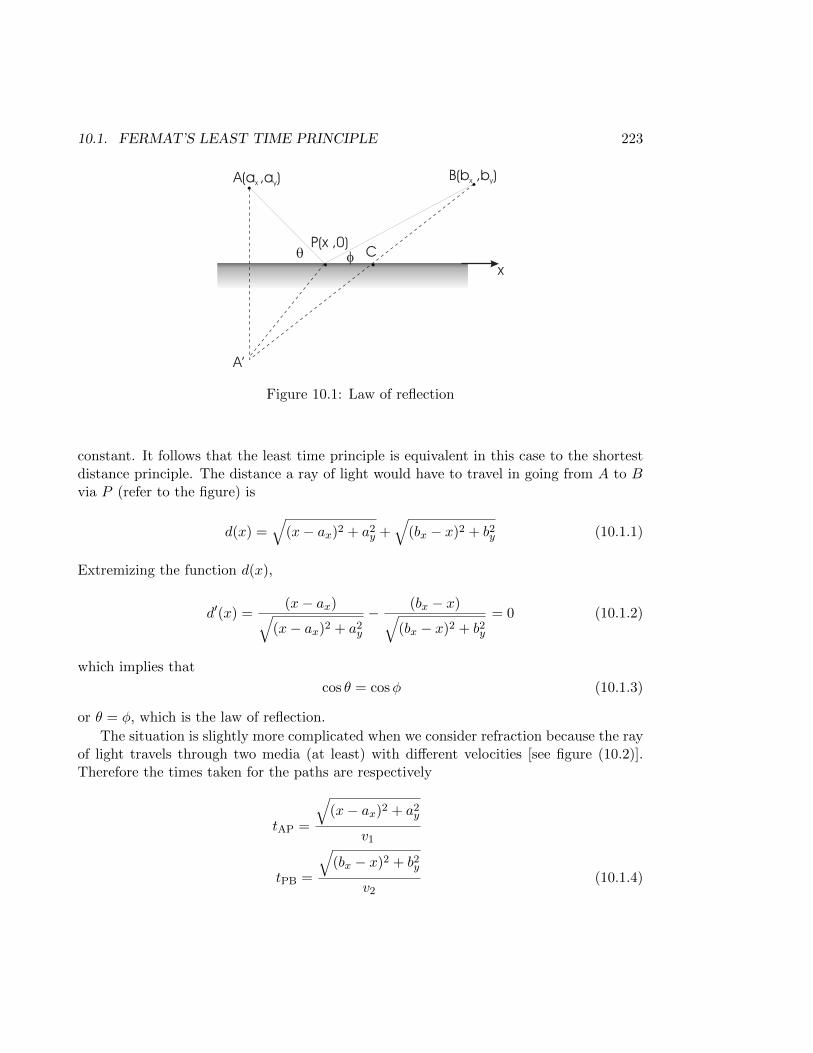
10.1. FERMAT’S LEAST TIME PRINCIPLE 223
A(a ,a )x y
A’
B(b ,b )x y
P(x ,0)q f C
x
Figure 10.1: Law of reflection
constant. It follows that the least time principle is equivalent in this case to the shortestdistance principle. The distance a ray of light would have to travel in going from A to Bvia P (refer to the figure) is
d(x) =√
(x− ax)2 + a2y +
√(bx − x)2 + b2y (10.1.1)
Extremizing the function d(x),
d′(x) =(x− ax)√
(x− ax)2 + a2y
− (bx − x)√(bx − x)2 + b2y
= 0 (10.1.2)
which implies that
cos θ = cosφ (10.1.3)
or θ = φ, which is the law of reflection.
The situation is slightly more complicated when we consider refraction because the rayof light travels through two media (at least) with different velocities [see figure (10.2)].Therefore the times taken for the paths are respectively
tAP =
√(x− ax)2 + a2
y
v1
tPB =
√(bx − x)2 + b2y
v2(10.1.4)
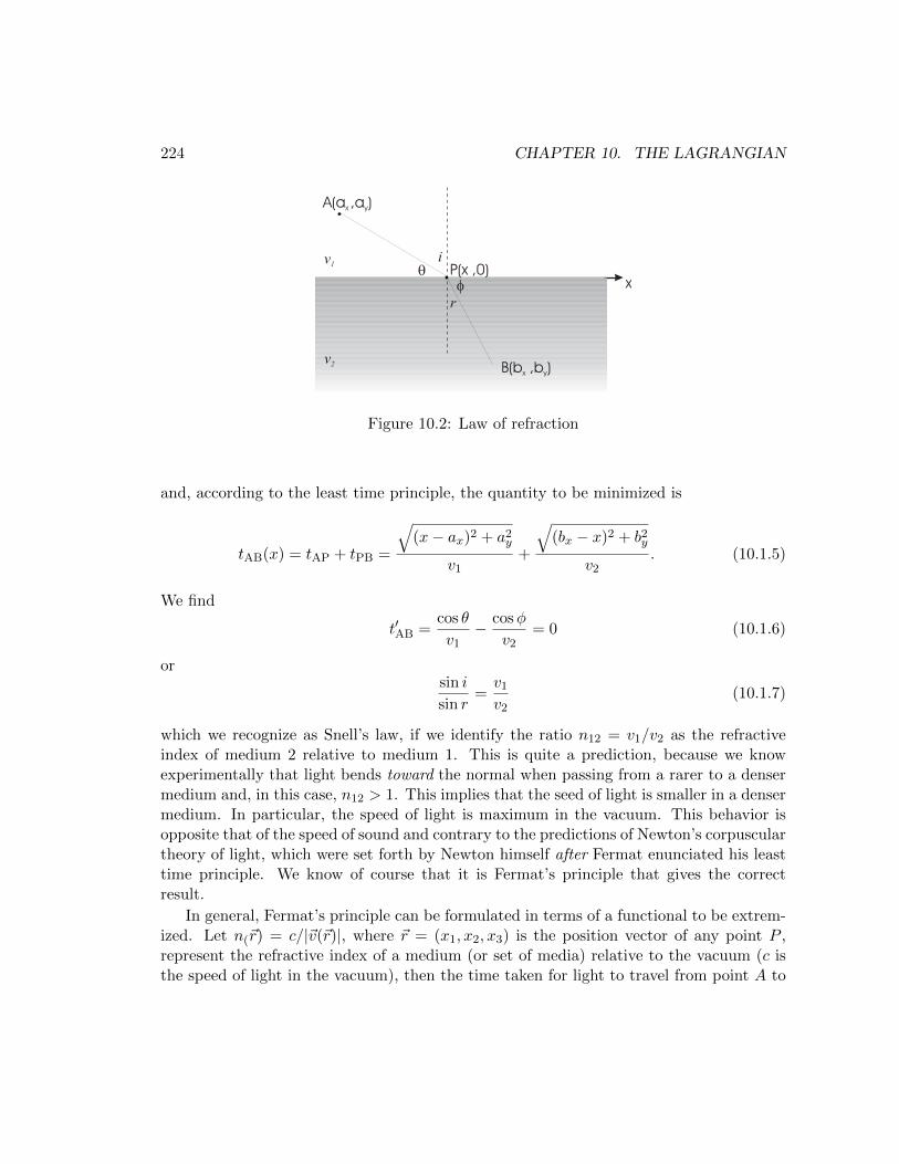
224 CHAPTER 10. THE LAGRANGIAN
A(a ,a )x y
B(b ,b )x y
P(x ,0)qf x
v2
v1
i
r
Figure 10.2: Law of refraction
and, according to the least time principle, the quantity to be minimized is
tAB(x) = tAP + tPB =
√(x− ax)2 + a2
y
v1+
√(bx − x)2 + b2y
v2. (10.1.5)
We find
t′AB =cos θ
v1− cosφ
v2= 0 (10.1.6)
orsin i
sin r=v1
v2(10.1.7)
which we recognize as Snell’s law, if we identify the ratio n12 = v1/v2 as the refractiveindex of medium 2 relative to medium 1. This is quite a prediction, because we knowexperimentally that light bends toward the normal when passing from a rarer to a densermedium and, in this case, n12 > 1. This implies that the seed of light is smaller in a densermedium. In particular, the speed of light is maximum in the vacuum. This behavior isopposite that of the speed of sound and contrary to the predictions of Newton’s corpusculartheory of light, which were set forth by Newton himself after Fermat enunciated his leasttime principle. We know of course that it is Fermat’s principle that gives the correctresult.
In general, Fermat’s principle can be formulated in terms of a functional to be extrem-ized. Let n(~r) = c/|~v(~r)|, where ~r = (x1, x2, x3) is the position vector of any point P ,represent the refractive index of a medium (or set of media) relative to the vacuum (c isthe speed of light in the vacuum), then the time taken for light to travel from point A to
10.2. THE VARIATIONAL PRINCIPLE OF MECHANICS 225
point B is the functional
T [x1, x2, x3] =
∫ B
A
ds
|~v(~r)|=
1
c
∫ B
An(~r)ds (10.1.8)
According to Fermat’s principle, the path followed by a ray of light is the one for whichT [x1, x2, x3] is minimum. The functional T [x1, x2, x3] is called the optical path lengthfrom A to B.
10.2 The variational principle of mechanics
In the previous chapter we saw that minimization of the path length yields straight linetrajectories but not Newton’s first law. This was because reparameterization invarianceimplied that Euler’s equations cannot determine the speed of the particle, only the curva-ture of its trajectory. To recover the entire content of the first law from Euler’s equations,we could introduce a constraint requiring that the speed is held fixed, but the constraintwould be non-holonomous and non-holonomous constraints are usually difficult to dealwith. Moreover, this cannot be the correct approach because the constraint could notbe imposed in the presence of external forces and we are, in the end, after a variationalprinciple for a particle or system of particles in the presence of external and internal forces.We would therefore encounter a situation in which the functional describing the motionof a free particle cannot be obtained as the limit of a more general functional as the ex-ternal forces are made to vanish. Therefore, we ask instead if there is a functional whoseextremization would yield
mxi = 0, i ∈ 1, 2, 3 (10.2.1)
(the equations of motion for a free particle) without imposing additional constraints. It isnot difficult to see that the equations xi = 0 extremize the functional
S′ =
∫ 2
1dt
1
2
∑i
x2i , (10.2.2)
therefore, since we want mxi = 0, or more precisely dpi/dt = 0, we simply multiply thefunctional S′ by the mass of the particle, taking instead the action
S =
∫ 2
1dt
1
2m∑i
x2i =
∫ 2
1dt T (xi). (10.2.3)
where we recognize T (xi) to be the kinetic energy of the particle.Notice that the motion of a free particle is not interpreted as optimizing any geometric
quantity (such as the path length) but rather the average kinetic energy of the particle.
226 CHAPTER 10. THE LAGRANGIAN
However, it turns out that it is actually an approximation of a quantity that does havea geometric meaning, the “proper time” of the particle. This is the time measured on aclock that moves with the particle. For observers relative to whom the speed of the particleis slow compared with the speed of light the proper time approximates to the absolute,Galilean, time up to corrections of order v2/c2. The functional (10.2.3) represents the firstcorrection term.
Including the action of forces on the particle (Newton’s second law) just as easy. ModifyS by introducing an additional function
S =
∫ 2
1dt [T (xi) + Z(xi, xi, t)] (10.2.4)
and determine Z. The Euler Lagrange equations are then
−mxi +∂Z
∂xi− d
dt
(∂Z
∂xi
)= 0. (10.2.5)
We will consider only forces that are derivable from a potential, Fi = −∂iU (conservativeforces). If the force does not depend on the velocity then the potential is a function onlyof position, U = U(~r). According to Newton’s second law, mxi = −∂iU , therefore wemust take Z(xixi, t) = −U(xi). Therefore, when all the forces acting on the particle areconservative, extremizing the functional
S =
∫ 2
1dt [T (xi)− U(xi)] (10.2.6)
then gives precisely Newton’s second law of motion. As is often the case in physics, we raisethe statement to the status of a fundamental law, applicable to all physical systems andgeneralizing when necessary even Newton’s three laws of motion, leaving it to experimentto determine its the limits if any of its validity. Thus we arrive at Hamilton’s principle(which has yet to be challenged):
Hamilton’s principle: Of all possible paths along which a dynamical system may evolve,from one configuration to another within a fixed time interval, the actual path taken isthe one that extremizes the functional (10.2.6).
The quantity L = T − U is called the Lagrangian of the system and S is called theaction functional,
S =
∫ 2
1dt L(xi, xi, t) (10.2.7)
When a system consists of more than one particle, the kinetic energy is the total kineticenergy, i.e., the simple sum of kinetic energies of the individual particles and the potentialenergy is the total potential energy (external plus internal) of the system.
10.2. THE VARIATIONAL PRINCIPLE OF MECHANICS 227
When there are constraints on a system, the coordinates and velocities are not allindependent. In the case of holonomous constraints this is resolved by choosing a set ofgeneralized coordinates that solve the constraints. For an unconstrained n particlesystem there are 3n coordinates, xi. Imposing r constraints reduces the number of in-dependent coordinates to 3n − r. If the constraints can be solved so that the Cartesiancoordinates, or a subset of them, are expressed in terms of 3n− r generalized coordinates,qa ∈ q1, q2, . . . , q3n−r then we will have 2n relations of the form
xi = xi(q1, q2, ..., q3n−r), xi =
3n−r∑a=1
∂xi∂qa
qa (10.2.8)
The Lagrangian may be expressed in terms of the geneneralized coordinates without con-straints. If it is impossible to find generalized coordinates (because it turns out to beexceedingly difficult to solve the constraints) then the Lagrangian may be written in termsof the original coordinates, xi, with the constraints introduced via Lagrange multipliers.One should use Lagrange multipliers only as a last resort. Solving and eliminating theconstraints first is always preferred, when possible.
When the constraints are of the form
gα(xi, xi, t) = 0 (10.2.9)
one should first check if they are integrable. For example, the constraint∑i
Ai(~x, t)dxidt
+B(~x, t) (10.2.10)
is integrable if and only if ∑i
Ai(~x, t)dxi +B(~x, t)dt = df(~x, t) (10.2.11)
where f is some function of xi and t. This means that
Ai =∂f
∂xiB =
∂f
∂t(10.2.12)
for some function f(~x, t) and it follows that
∂Ai∂t
=∂B
∂xi(10.2.13)
If these conditions fail the constraint is not holonomous.
228 CHAPTER 10. THE LAGRANGIAN
10.3 Examples
The one dimensional harmonic oscillator is described by the potential function U(x) =12kx
2. Its Lagrangian is therefore
L = T (x)− U(x) =1
2
(mx2 − kx2
)(10.3.1)
with the action
S =1
2
∫ 2
1dt(mx2 − kx2). (10.3.2)
The Euler equation,∂L∂x− d
dt
(∂L∂x
)= −kx−mx = 0 (10.3.3)
yields the well known equation of motion mx = −kx.
The gravitational potential energy of a system of two particles of mass m1 and m2 isU(r) = −Gm1m2m/|~r1 − ~r2|. The Lagrangian therefore is
L =1
2m1~r1
2+
1
2m2~r2
2+Gm1m2
|~r1 − ~r2|, (10.3.4)
and the action,
S =
∫ 2
1dt
[1
2m1~r1
2+
1
2m2~r2
2+Gm1m2
|~r1 − ~r2|
](10.3.5)
when extremized gives the Euler equations
∂L∂xn,i
− d
dt
(∂L∂xn,i
)= 0 (10.3.6)
or
m1~r1 = −Gm1m2(~r1 − ~r2)
|~r1 − ~r2|3
m2~r2 = −Gm1m2(~r2 − ~r1)
|~r1 − ~r2|3(10.3.7)
which together represent the familiar Newton’s law of universal gravitation.
Consider the simple pendulum shown in figure (10.3). Begin by using the Cartesiancoordinates of the bob, in terms of which
T =1
2m(x2 + y2) (10.3.8)

10.3. EXAMPLES 229
O
y
x
(x ,y)
q
Figure 10.3: The simple pendulum
and U(y) = mgy. There is one holonomous constraint on the system, which is that thelength of the cord is held fixed during the motion
g(x, y) =√x2 + y2 − l. (10.3.9)
So we have a choice. We could incorporate the constraint in an action,
Sλ =
∫ 2
1dt
[1
2m(x2 + y2)−mgy + λ(t)(
√x2 + y2 − l)
], (10.3.10)
or we could choose to solve the constraints by reparameterizing the problem via the in-vertible transformation
x = l sin θ, y = l cos θ (10.3.11)
in which case we calculate
T =1
2ml2θ2 (10.3.12)
and therefore we could write a action functional of just one dependent function
S =
∫ 2
1dt
[1
2ml2θ2 +mgl cos θ
](10.3.13)
The equations of motion for this system are
−mgl sin θ −ml2θ = 0 ⇒ θ = −gl
sin θ (10.3.14)
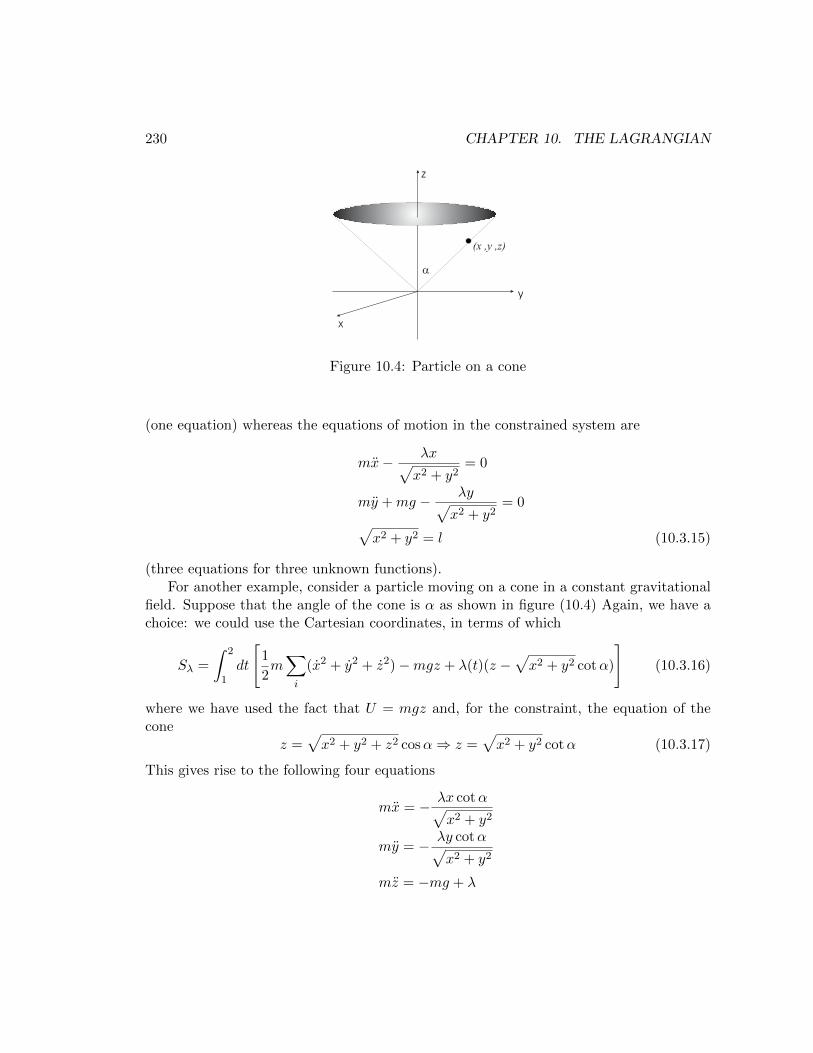
230 CHAPTER 10. THE LAGRANGIAN
z
y
a
(x ,y ,z)
x
Figure 10.4: Particle on a cone
(one equation) whereas the equations of motion in the constrained system are
mx− λx√x2 + y2
= 0
my +mg − λy√x2 + y2
= 0√x2 + y2 = l (10.3.15)
(three equations for three unknown functions).For another example, consider a particle moving on a cone in a constant gravitational
field. Suppose that the angle of the cone is α as shown in figure (10.4) Again, we have achoice: we could use the Cartesian coordinates, in terms of which
Sλ =
∫ 2
1dt
[1
2m∑i
(x2 + y2 + z2)−mgz + λ(t)(z −√x2 + y2 cotα)
](10.3.16)
where we have used the fact that U = mgz and, for the constraint, the equation of thecone
z =√x2 + y2 + z2 cosα⇒ z =
√x2 + y2 cotα (10.3.17)
This gives rise to the following four equations
mx = − λx cotα√x2 + y2
my = − λy cotα√x2 + y2
mz = −mg + λ
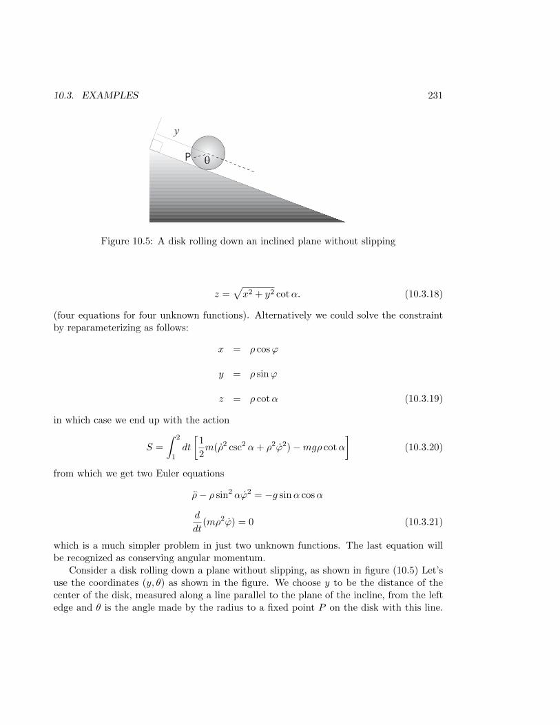
10.3. EXAMPLES 231
y
P q
Figure 10.5: A disk rolling down an inclined plane without slipping
z =√x2 + y2 cotα. (10.3.18)
(four equations for four unknown functions). Alternatively we could solve the constraintby reparameterizing as follows:
x = ρ cosϕ
y = ρ sinϕ
z = ρ cotα (10.3.19)
in which case we end up with the action
S =
∫ 2
1dt
[1
2m(ρ2 csc2 α+ ρ2ϕ2)−mgρ cotα
](10.3.20)
from which we get two Euler equations
ρ− ρ sin2 αϕ2 = −g sinα cosα
d
dt(mρ2ϕ) = 0 (10.3.21)
which is a much simpler problem in just two unknown functions. The last equation willbe recognized as conserving angular momentum.
Consider a disk rolling down a plane without slipping, as shown in figure (10.5) Let’suse the coordinates (y, θ) as shown in the figure. We choose y to be the distance of thecenter of the disk, measured along a line parallel to the plane of the incline, from the leftedge and θ is the angle made by the radius to a fixed point P on the disk with this line.
232 CHAPTER 10. THE LAGRANGIAN
The kinetic energy of the disk is the kinetic energy of its center of mass together with itsrotational kinetic energy
T =1
2My2 +
1
2Iθ2 (10.3.22)
and its potential energy is just gravitational, U = mgh = mg(L− y) sinα, where L is thelength of the incline and α is its angle.
However, this is not enough because we must also incorporate the constraint that thedisk does not slip. This means that dy = Rdθ where R is the radius of the disk. We couldinclude a constraint,
Sλ =
∫ 2
1dt
[1
2My2 +
1
2Iθ2 −mg(L− y) sinα+ λ(y − y0 −Rθ)
](10.3.23)
and solve the three equations,
My = mg sinα+ λ
Iθ = −Rλ
y = y0 +Rθ, (10.3.24)
for the three unknown functions, y(t), θ(t) and λ(t). Alternatively, we could incorporatethe constraint directly:
T =1
2(MR2 + I)θ2 =
1
2I ′θ2
U = mg(L− y0 −Rθ) (10.3.25)
so that
S =
∫ 2
1dt
[1
2I ′θ2 −mg(L− y0 −Rθ) sinα
](10.3.26)
giving the single Euler equation
I ′θ = mgR sinα, (10.3.27)
for θ(t).1
1Suggestion: It’s a good exercise to go through mechanics problems from elementary textbooks, say onCalculus based first year Physics, and set up Lagrangians describing the systems with careful attention tothe constraints. Verify, in each case, that the equations of motion obtained from the traditional approach(m~a = ~F , I~α = ~τ) are equivalent to the Euler equations extremizing the Lagrangians.
10.4. SYMMETRIES AND NOETHER’S THEOREMS 233
10.4 Symmetries and Noether’s theorems
E. Noether’s two theorems, the first relating the conservation laws to the existence of globalsymmetries (finite, continuous group symmetries of the action) and the second pointingout the existence of identities that result from local symmetries (infinite, continuous groupsymmetries of the action), profoundly influenced the course of physics in the 20th century,leading eventually to the discovery of gauge theories in particle physics. In this sectionwe will prove both Noether’s first and most well-known theorem in general, as well asher second theorem but only for a special class of local transformations. Both proofs willbe given in the context of particle mechanics, but their extension to “field” theories isstraightforward.
Consider a general action,
S =
∫ 2
1dt L(qi, qi; t), (10.4.1)
where L(q, q; t) includes all constraints (solved via generalized coordinates or not) andconsider a transformation of time, say t → t′ = t + δt = t + ε(t) and the coordinates,q(t) → q′(t′) = q(t) + δq(t). The action is invariant under this transformation if δS = 0.So far we have only been concerned with variations in which δt = 0. When δt 6= 0, thetotal change in the coordinates is the sum of two parts, the first arising due to a changein the argument, t, of the coordinates and the second due to a change in the functionalform of q(t), which is what we used up to now and which, to avoid confusion with thetotal change in q(t), we will henceforth represent by δ0q(t):
δ0q(t) = q′(t)− q(t) = αη(t) (10.4.2)
where η(t) are arbitrary functions of t, earlier taken to vanish at the boundaries. Notethat a variation of the functional form of qi(t) and differentiation with respect to time areindependent operations, which can be performed in any order,i.e.,
[δ0,d
dt] = 0. (10.4.3)
Thus, for δt 6= 0,
q(t)→ q′(t′) = q(t′) + δ0q(t′) = q(t+ ε) + δ0q(t) (10.4.4)
where, in the second term on the right, we have ignored a second order correction, giventhat the transformations are infinitesimal. For each coordinate in L, we can write
q′(t′) = q(t) + ε(t)q(t) + δ0q(t), (10.4.5)
234 CHAPTER 10. THE LAGRANGIAN
which givesδq(t) = ε(t)q(t) + δ0q(t) (10.4.6)
where δq(t) is the total variation of q(t).2 In the same way, noting that
q′(t′) =d
dt′q′(t′) =
dt
dt′d
dt[q(t) + ε(t)q(t) + δ0q(t)]
= (1− ε(t))[q(t) + ε(t)q(t) + ε(t)q(t) + δ0q(t)] (10.4.7)
we find, to first order in the variations,
q′(t′) = q(t) + ε(t)q(t) + δ0q(t), (10.4.8)
orδq(t) = ε(t)q(t) + δ0q(t). (10.4.9)
The change induced in S by the variations just described is
δS =
∫ 2
1[δ(dt)L(qi, qi; t) + dtδL(qi, qi; t)] (10.4.10)
Nowt→ t′ = t+ ε(t)⇒ dt→ dt′ = [1 + ε(t)]dt (10.4.11)
orδ(dt) = ε(t)dt (10.4.12)
and therefore
δS =
∫ 2
1dt
[ε(t)L+ ε(t)
∂L∂t
+∑i
∂L∂qi
δqi +∑i
∂L∂qi
δqi
]. (10.4.13)
Substituting the total variations of q(t) and q(t), given in (10.4.6) and (10.4.9), we find
δS =
∫ 2
1dt
[εL+ ε
∂L∂t
+∑i
∂L∂qi
(εqi + δ0qi) +∑i
∂L∂qi
(εqi + δ0qi)
](10.4.14)
which expression, collecting terms proportional to ε, simplifies to
δS =
∫ 2
1dt
[d
dt(εL) +
∑i
∂L∂qi
δ0qi +∑i
∂L∂qi
δ0qi
]. (10.4.15)
2Problem: Show that the total variation of qi(t) does not commute with the differentiation with respectto time, [
δ,d
dt
]qi(t) 6= 0.
10.4. SYMMETRIES AND NOETHER’S THEOREMS 235
The last term in the integrand of (10.4.15) can be re-expressed using,∑i
[d
dt
(∂L∂qi
δ0qi
)− d
dt
(∂L∂qi
)δ0qi
](10.4.16)
and we find
δS =
∫ 2
1dt
[∑i
Eiδ0qi +d
dt
(εL+
∑i
∂L∂qi
δ0qi
)](10.4.17)
where Ei is the Euler derivative of L. If the variations are required to vanish on theboundaries, then the surface term vanishes and the action is invariant (δS = 0) providedthat ∑
i
∫ 2
1dtEiδ0qi = 0 (10.4.18)
This will be recognized as precisely (9.2.16). The action is also invariant under the trans-formations that do not vanish on the boundaries, provided that each term vanishes, i.e.,both Ei = 0 (Euler’s equations) and
d
dt
(εL+
∑i
∂L∂qi
δ0qi
)= 0 (10.4.19)
hold true simultaneously. This is saying that the quantity in brackets is a constant of themotion, so it is a conservation law. Let us first re-express the conserved quatity above interms of the total variations, using (10.4.6), as(
L −∑i
∂L∂qi
qi
)ε+
∑i
∂L∂qi
δqi = const. (10.4.20)
and suppose that the variations result from some global transformations which form afinite, continuous group and depend on r constant parameters, δωa, a ∈ 1, 2, ..., r,according to
δt = ε(t) = Ga(t)δωa ⇒ Ga =δε(t)
δωa
δqi(t) = Gia(q, t)δωa,⇒ Gia =δqiδωa
. (10.4.21)
The G’s are called the generators of the transformation. Inserting these into (10.4.21), wefind that the r quantities
ja =
(L −
∑i
∂L∂qi
qi
)Ga +
∑i
∂L∂qiGia (10.4.22)
236 CHAPTER 10. THE LAGRANGIAN
are conserved on the physical trajectories, i.e., so long as Euler’s equations are obeyed.This is Noether’s first and most famous theorem. Below are some simple but very specialexamples of how it works in the context of particle mechanics.
• Time translations: Take a translation of time by a constant, t → t′ = t + δω andqi(t)→ q′i(t
′) = qi(t) (trajectories do not depend on the choice of the time origin) soδqi = 0. This is a one parameter group of transformations in which G = 1, Gi = 0.If S is invariant under time translations, δS = 0 and
H =∂L∂qi
qi − L (10.4.23)
is a constant of the motion. H is called the “Hamiltonian” of the system and itcan, under certain conditions, be interpreted as the energy of the system. Energyconservation is thus a consequence of time translation invariance.
• Spatial translations: Constant translations of r coordinates, qi → qi+ai holding timefixed, t → t′(t) = t form an r dimensional Abelian group with δωi = ai = δqi andε(t) = 0, or Gi = 0 and Gij = δij . If the action is invariant under spatial translationsof some or all of the N coordinates then for those coordinates,
pi =∂L∂qi
(10.4.24)
is conserved. pi is called the momentum of the system “conjugate” to qi.3 Thus
momentum conservation in any direction is a consequence of space translation in-variance of the action. A coordinate that does not appear in the Lagrangian i.e.,upon which the Lagrangian does not explicitly depend is called cyclic or ignorable.Naturally, the momentum conjugate to a cyclic coordinate is conserved.
• Spatial Rotations: Finally, let the coordinates qi represent the usual Cartesian co-ordinates, and use xi instead to denote them. General rotations of the coordinate
3In the simple example in which
L =∑i
1
2mx2i − U(xi)
we find that∂L∂xi
= mxi
which is precisely the momentum of the system. We generalize this to any system by simply declaring∂L/∂qi to be the momentum of the system conjugate to the (possibly generalized) coordinate qi. TheHamiltonian is generally expressed in terms of the generalized momentum as
H =∑i
piqi − L.
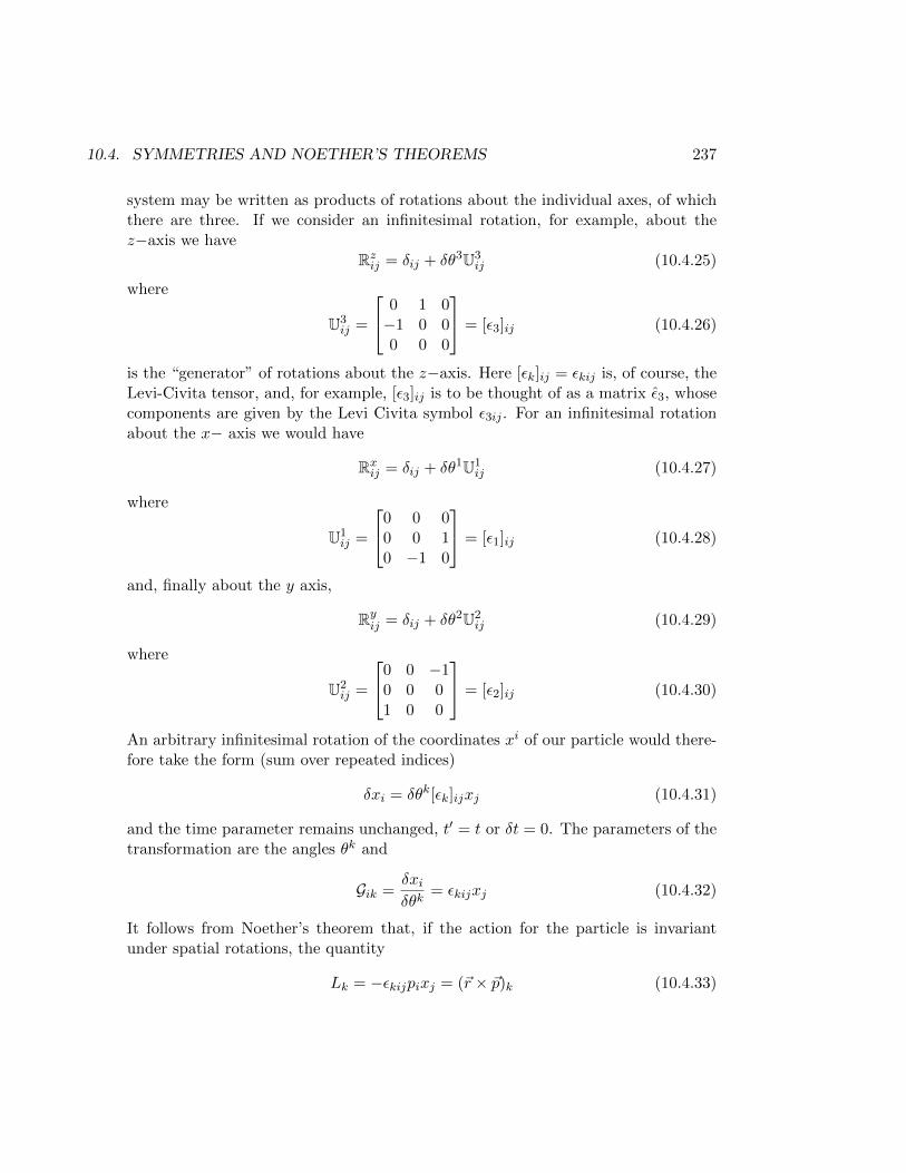
10.4. SYMMETRIES AND NOETHER’S THEOREMS 237
system may be written as products of rotations about the individual axes, of whichthere are three. If we consider an infinitesimal rotation, for example, about thez−axis we have
Rzij = δij + δθ3U3ij (10.4.25)
where
U3ij =
0 1 0−1 0 00 0 0
= [ε3]ij (10.4.26)
is the “generator” of rotations about the z−axis. Here [εk]ij = εkij is, of course, theLevi-Civita tensor, and, for example, [ε3]ij is to be thought of as a matrix ε3, whosecomponents are given by the Levi Civita symbol ε3ij . For an infinitesimal rotationabout the x− axis we would have
Rxij = δij + δθ1U1ij (10.4.27)
where
U1ij =
0 0 00 0 10 −1 0
= [ε1]ij (10.4.28)
and, finally about the y axis,
Ryij = δij + δθ2U2ij (10.4.29)
where
U2ij =
0 0 −10 0 01 0 0
= [ε2]ij (10.4.30)
An arbitrary infinitesimal rotation of the coordinates xi of our particle would there-fore take the form (sum over repeated indices)
δxi = δθk[εk]ijxj (10.4.31)
and the time parameter remains unchanged, t′ = t or δt = 0. The parameters of thetransformation are the angles θk and
Gik =δxiδθk
= εkijxj (10.4.32)
It follows from Noether’s theorem that, if the action for the particle is invariantunder spatial rotations, the quantity
Lk = −εkijpixj = (~r × ~p)k (10.4.33)
238 CHAPTER 10. THE LAGRANGIAN
(which will be recognized as the angular momentum of the particle) is conserved.Conservation of angular momentum is a consequence of invariance of the actionunder spatial rotations.
Since the currents derived from (10.4.22) are conserved only on physical trajectories, theyare sometimes said to be weakly conserved and Noether’s first theorem is said to lead toweak conservation laws.
Noether’s second theorem deals with actions that are invariant under transformationsbelonging to an infinite, continuous group, i.e., transformations that are not just globalbut local, in which the variations ε and δqi depend of a finite number, r, of functions andtheir derivatives. It states that in general, and not simply on (physical) trajectories forwhich Euler’s equations hold, the local symmetries imply a set of r identities between theEuler derivatives of the Lagrangian.
According to (10.4.17), the action is invariant under the transformations if∫ 2
1dt
[∑i
Eiδ0qi +d
dt
(εL+
∑i
∂L∂qi
δ0qi
)]= 0, (10.4.34)
where the Ei are the Euler derivatives of L. For simplicity we will restrict ourselves hereto a special set of transformations, in which the variations depend on r functions δωa(t)and their first derivatives only,
ε(t) = Gaδωa(t)δqi(t) = Giaδωa(t) + Tiaδωa(t). (10.4.35)
Because the δωa are arbitrary functions of t, we can choose them so that they and theirderivatives vanish at the boundaries. In that case, the surface terms (total derivatives)automatically vanish and invariance implies that
∑i
∫ 2
1dt Ei(δqi − εqi) =
∑i
∫ 2
1dt Ei [(Gia − qiGa)δωa + Tiaδωa] = 0. (10.4.36)
Integrating the last term by parts, we find
∑i
∫ 2
1dt
[Ei(Gia − qiGa)−
d
dt(EiTia)
]δωa, (10.4.37)
which, for arbitrary δωa, is only possible if∑i
[Ei(Gia − qiGa)−
d
dt(EiTia)
]= 0 (10.4.38)
10.4. SYMMETRIES AND NOETHER’S THEOREMS 239
These r identities of Noether’s second theorem are trivially satisfied on physical trajectories(Ei = 0) but they hold irrespective of the Euler equations (they are strong) and, if theyare non-trivial, show that the Euler equations are not all independent. Although we havecarried out the calculation here for the special transformations in (10.4.35), the theoremitself is quite general and the same procedure may be employed when higher derivatives arepresent. Naturally, more complicated local symmetries lead to more complicated identities,but it all cases the existence of r identities implies that only (n − r) of the equations ofmotion are independent. Thus, like external constraints, local symmetries of the actionreduce the number of physical degrees of freedom in the system. As we saw earlier, forexample, the local reparameterization invariance of the path length functional in (9.6.5)implies that there are only two instead of three independent equations of motion.
Chapter 11
The Hamiltonian
The Lagrangian formulation adds considerably to our understanding of mechanics, both bycontributing to its philosophical underpinnings and by introducing a substantial amountof new mathematical structure, which, as we have seen, can be exploited to gain a moreprofound understanding of the general properties of a physical system. The Hamilto-nian formulation of mechanics is an alternative to the Lagrangian formulation. Whilenot adding in any way to the physics, it provides new mathematical structure and morepowerful ways of working with the physical principles that have already been established.
11.1 Legendre Transformations
From Noether’s first theorem, an action that is invariant under time translations describesa system that conserves the Hamiltonian
H =∂L∂qi
qi − L,dHdt
= 0. (11.1.1)
But, because
dLdt
=∂L∂qi
qi +∂L∂qi
qi +∂L∂t
=d
dt
(∂L∂qi
qi
)+∂L∂t
(11.1.2)
(where we have used Euler’s equation), (11.1.1) implies that
d
dt
(∂L∂qi
qi − L)
= −∂L∂t
= 0. (11.1.3)
240
11.1. LEGENDRE TRANSFORMATIONS 241
and it follows also that L can have no explicit dependence on time. For example, takea single particle of mass m moving in a potential U(~r) and let it be described by theLagrangian
L =1
2mx2
i − U(xi) (11.1.4)
where a summation over repeated indices is understood. We find
∂L∂xi
= mxi (11.1.5)
which is just the ith component of the momentum of the particle! The Hamiltonian is
H = mx2i −
1
2mx2
i + U(xi) =1
2mx2
i + U(xi) (11.1.6)
which will be recognized as the total energy of the particle. Because L does not explicitlydepend on time, the total energy of such a system is conserved.
Now we had defined the “generalized momentum” conjugate to the generalized coor-dinate qi by
pi =∂L∂qi
. (11.1.7)
If this system of equations is invertible then we may solve it to get the velocities in termsof the momenta and coordinates, qi = qi(q, p, t). Once this is done, the Hamiltonian canbe written in the form
H = piqi(q, p, t)− L. (11.1.8)
and it is easy to show that H = H(qi, pi, t) is independent of the velocities. The righthand side of (11.1.8) is a Legendre transformation of L, taking us from a function ofthe coordinates and velocities, L(qi, qi, t), to a function of the coordinates and momenta,H(qi, pi, t) .
Legendre transformations are performed often in physics. For example in Thermody-namics, going from the internal energy to the free energy of a system involves a Legendretransformation. The first law of Thermodynamics,
dU = TdS − pdV,
shows that U is naturally viewed as a function of (S, V ) and then T = (∂U/∂S)V . Bydefining the (Helmholz) free energy as F = U − TS, we make a Legendre transformationtaking U(S, V )→ F (T, V ), as one can check from
dF = dU − TdS − SdT = −pdV − SdT.
242 CHAPTER 11. THE HAMILTONIAN
This enables us to deal more effectively with situations in which the temperature andvolume are easy to control or measure. For example, while the work done by a thermody-namic system during an isentropic process is equal to the decrease in its internal energy,the work done during an isothermal process is equal to the decrease in its free energy.Another useful quantity with dimensions of energy is the enthalpy, H, which involves aLegendre transformation from U(S, V ) → H(S, p). Again, p = −∂U/∂V implies that thedesired Legendre transformation must be H = U + pV ,
dH = dU + pdV + V dp = TdS + V dp
In the same spirit, a double Legendre transformation would take us to the ThermodynamicPotential or Gibbs free energy, G(T, p) = U − TS + pV .
dG = −SdT + V dp
The Gibbs free energy stays constant during any process that is both isobaric and isother-mal, such as a phase transition.
11.2 The Canonical equations of motion
The Legendre transformation that takes us from the Lagrangian description to the Hamil-tonian replaces qi with pi so that H can be thought of as a function only of the coordinatesand momenta, not the velocities. The coordinates and momenta must be treated indepen-dently and, assuming there are n independent coordinates, they define a space that is 2ndimensional. This space of coordinates and momenta is called phase space.
The first step in performing the transformation involves using the definition of pi in(11.1.7) to obtain the velocities, qi, in terms of the coordinates and momenta, i.e., wesolve (11.1.7) for qi(qi, pi, t). In the next step we must replace the replace qi everywhereon the right hand side of (11.1.8) to recover H(qi, pi, t). By the inverse function theorem,however, the first step is only possible if
det|Wij | = det
∣∣∣∣∂pi∂qj
∣∣∣∣ = det
∣∣∣∣ ∂2L∂qi∂qj
∣∣∣∣ 6= 0. (11.2.1)
The matrix Wij is called the Hessian. When the determinant of the Hessian is non-vanishing the Lagrangian system is called regular, otherwise it is singular. When theLagrangian system is singular a Hamiltonian may be defined only on a subset of theoriginal phase space. This Hamiltonian may subsequently be extended over the entirephase space by explicitly introducing constraints in much the same way as we did earlierby means of Lagrange multipliers. The procedure was originally outlined by Dirac andlater elaborted upon by Bergmann. We will outline the Dirac-Bergmann algorithm at the
11.2. THE CANONICAL EQUATIONS OF MOTION 243
end of this chapter but, for the most part, we consider regular Lagrangian systems in thesenotes.
From the defining equations and the definition of the generalized momenta follow theequations of motion in terms of the Hamiltonian. Notice that from the definition of H in(11.1.8),
dH = qidpi + pidqi −∂L∂tdt− ∂L
∂qidqi −
∂L∂qi
dqi
= qidpi −∂L∂qi
dqi −∂L∂tdt, (11.2.2)
where we used the definition of the generalized momenta. This shows that H = H(qi, pi, t)and therefore
dH =∂H∂pi
dpi +∂H∂qi
dqi +∂H∂t
dt. (11.2.3)
Comparing the two expressions we see that
qi =∂H
∂pi∂L∂qi
= −∂H∂qi
∂L∂t
= −∂H∂t
(11.2.4)
But, by Euler’s equations,∂L∂qi
=d
dt
(∂L∂qi
)= pi (11.2.5)
so we find that the set of equations in (11.2.4) can also be written as
qi =∂H
∂pi, pi = −∂H
∂qi,∂L∂t
= −∂H∂t
. (11.2.6)
These are known as the Hamilton equations (of motion). Using them we find that
dHdt
=∂H∂t
+∂H∂qi
qi +∂H∂pi
pi =∂H∂t
(11.2.7)
which says that any time dependence of the Hamiltonian must be explicit.The Hamilton equations are also called the canonical equations of motion and
the description of the motion by them is called Hamiltonian dynamics. If there are ngeneralized coordinates, there must be 2n pairs (qi, pi) and 2n canonical equations. Thecanonical equations are coupled, first order differential equations in time whose integration
244 CHAPTER 11. THE HAMILTONIAN
involves 2n constants or initial values. This is the same number of constants that arerequired for Lagrangian dynamics because, although there are just n Euler equations theyare second order in time. The space formed by all the generalized coordinates is called theconfiguration space of the system. The space formed by all the generalized coordinatesand momenta is called the phase space or momentum state space of the system. Thespace formed by all the generalized coordinates and their corresponding velocities is calledthe velocity state space of the system.
11.3 Poisson Brackets
Observables in the Hamiltonian description will consist of functions of the coordinates,momenta and time, A = A(qi, pi, t). Given two observables A and B we define the PoissonBrackets of A and B as
A,BPBdef=
∑k
(∂A
∂qk
∂B
∂pk− ∂A
∂pk
∂B
∂qk
)(11.3.1)
The Poisson brackets have several features of considerable interest. In particular, if wetake A = qi and B = pj , we find that
qi, pjPB =∑l
δilδlj = δij
qi, qjPB = 0 = pi, pjPB (11.3.2)
These are called the “fundamental” Poisson brackets. Again, if we consider the time rateof change of any observable A,
dA
dt=∂A
∂qiqi +
∂A
∂pipi +
∂A
∂t(11.3.3)
and insert the canonical equations of motion, we find that
dA
dt=∂A
∂qi
∂H∂pi− ∂A
∂pi
∂H∂qi
+∂A
∂t(11.3.4)
ordA
dt= A,HPB +
∂A
∂t. (11.3.5)
An observable that satisfies dA/dt = 0 is called a constant of the motion. We see thatfor an observable not explicitly dependent on time to be a constant of the motion it musthave vanishing Poisson brackets with H. On the other hand, if A is a constant of themotion but does explicitly depend on time then ∂A/∂t = −A,HPB.
11.3. POISSON BRACKETS 245
We might take A to be just qi or pi, to find an alternative description of the canonicalequations of motion
qi = qi,HPB, pi = pi,HPB, (11.3.6)
in terms of Poisson brackets. Although the Poisson Bracket appears to be merely aconvenient notation, one should really think of it as a binary operation between observableswhich turns out to be of central importance in analytical mechanics. This will becomeclearer as we go along.
From now on, we will drop the subscript “PB” on the curly brackets unless they arerequired for clarity. Let’s list some of the properties of the Poisson Bracket. Each of thesecan be proved by starting from definition (11.3.1).
1. It is antisymmetric,
A,B = −B,A (11.3.7)
2. It is linear: if a and b are constants then
aA+ bB,C = aA,C+ bB,C (11.3.8)
3. For any constant, c, and any observable A, c, A = 0.
4. It satisfies the Jacobi Identity,
A, B,C+ CA,B+ BC,A = 0 (11.3.9)
(cyclic permtations of the observables).
5. It obeys the following product rule,
AB,C = A,CB +AB,C (11.3.10)
If only the first four conditions are obeyed by some binary operation between observablesthen it is called a “generalized Poisson Bracket”.
Two facts concerning observables are worthy of note. The first has to do with theconstruction of new invariants of the motion from old ones and the second has to do withthe approximate solution of the evolution equations for any function on phase space.
• Knowing any two constants of the motion, it is possible in principle to construct newconstants of the motion as follows: take C = H in the Jacobi identity,
A,B,H+ H, A, B+ B,H, A = 0
⇒ A,B,H+ ∂A∂t,B − ∂B
∂t,A = 0
246 CHAPTER 11. THE HAMILTONIAN
⇒ A,B,H+ ∂A∂t,B+ A, ∂B
∂t = 0
⇒ A,B,H+∂
∂tA,B = 0 (11.3.11)
showing that A,B is also a constant of the motion.1 In practice this method isnot very useful because the Poisson brackets of A and B often give trivial functionsor even constants.
• If an A does not depend explicitly on time and is well behaved, one can use thePoisson brackets to find a formal solution to its evolution equation
dA
dt= A,H. (11.3.12)
Expand A as a Taylor series
A(t) =∞∑n=0
A(n)(t0)
n!(t− t0)n (11.3.13)
where A(n) is the nth time derivative of A, and notice that
A(1)(t0) = A,H(t0)
A(2)(t0) = A(1),H(t0) = A,H,H(t0)
A(3)(t0) = A(1),H(t0) = A,H,H,H(t0)
. . .
A(n)(t0 = . . . A,H,H, . . . n times(t0) (11.3.14)
giving the following (formal) solution for the observable A
A(t) =∞∑n=0
1
n!. . . A,H,H, . . . n times(t0)(t− t0)n. (11.3.15)
In all but the simplest cases, this method cannot be applied to obtain exact solutions.However, it is quite useful in perturbation theory.
1Problem: Prove that
∂A∂t,B+ A, ∂B
∂t =
∂
∂tA,B
11.4. EXAMPLES 247
11.4 Examples
Consider the one dimensional system whose Hamiltonian is
H =p2
2− 1
2q2(11.4.1)
which you can think of as a particle of unit mass moving in the potential of a central,inverse cube force. The equations of motion for the particle are
q = q,H = p, p = p,H = − 1
q3(11.4.2)
which also give the (Euler) equation
q = − 1
q3. (11.4.3)
The quantity D = pq/2−Ht is a constant of the motion 2
dD
dt= D,H+
∂D
∂t=p
2
q,p2
2
+q
2
p,− 1
2q2
−H = 0, (11.4.4)
whose origin lies in the invariance of the system under a scale transformation,
q → Q = λq, t→ τ = λ2t, p→ P =p
λ. (11.4.5)
Invariance can be verified either from the canonical equations of motion, which remainunchanged in form,
dq
dt= λ
dQ
dτ= p = λP ⇒ dQ
dτ= P
dp
dt= λ3dP
dτ= − 1
q3= − λ
3
Q3⇒ dP
dτ= − 1
Q3(11.4.6)
or from the action for this system
S =
∫ 2
1dtL(q, q, t) =
∫ 2
1dt
(q2
2+
1
2q2
). (11.4.7)
2Problem: Generalize this: show that
D =~p · ~rn−Ht
is a constant of the motion for a Hamiltonian of the form H = |~p|n − ar−n where a is any constant.
248 CHAPTER 11. THE HAMILTONIAN
where now only the transformations of q and t need be specified. Noether’s first theoremthen implies that
j =
(L − ∂L
)δt
δλ+∂L∂q
δq
δλ= p
δq
δλ−H δt
δλ(11.4.8)
is conserved. Taking an infinitesimal scaling, λ = 1 + δλ, and evaluating j, we find
j = pq − 2Ht = 2D. (11.4.9)
The simple harmonic oscillator is such a simple physical system that the iterativemethod that was described in the previous section can actually be used to obtain an exactsolution. We have
L =1
2(mx2 − kx2)
p =∂L∂x
= mx⇒ x =p
m
H = px− L =p2
m− p2
2m+
1
2kx2 =
p2
2m+
1
2kx2 (11.4.10)
The equations of motion are
p = p,H =k
2p, x2 = −kx
x = x,H =1
2mx, p2 =
p
m(11.4.11)
To find x = x(t), we need to compute
x(2) = x,H = x,H,H =1
mp,H = − k
mx
x(3) = x(2),H = − kpm2
x(4) = x(3),H = +k2x
m2
... (11.4.12)
and so on. If we call set t0 = 0 and let x0 = x(0) and p0 = p(0) then (11.3.15) will givethe series solution
x(t) = x0 +p0
mt− kx0
mt2 − kp0
m2t3 +
k2x0
m2t4 + . . .
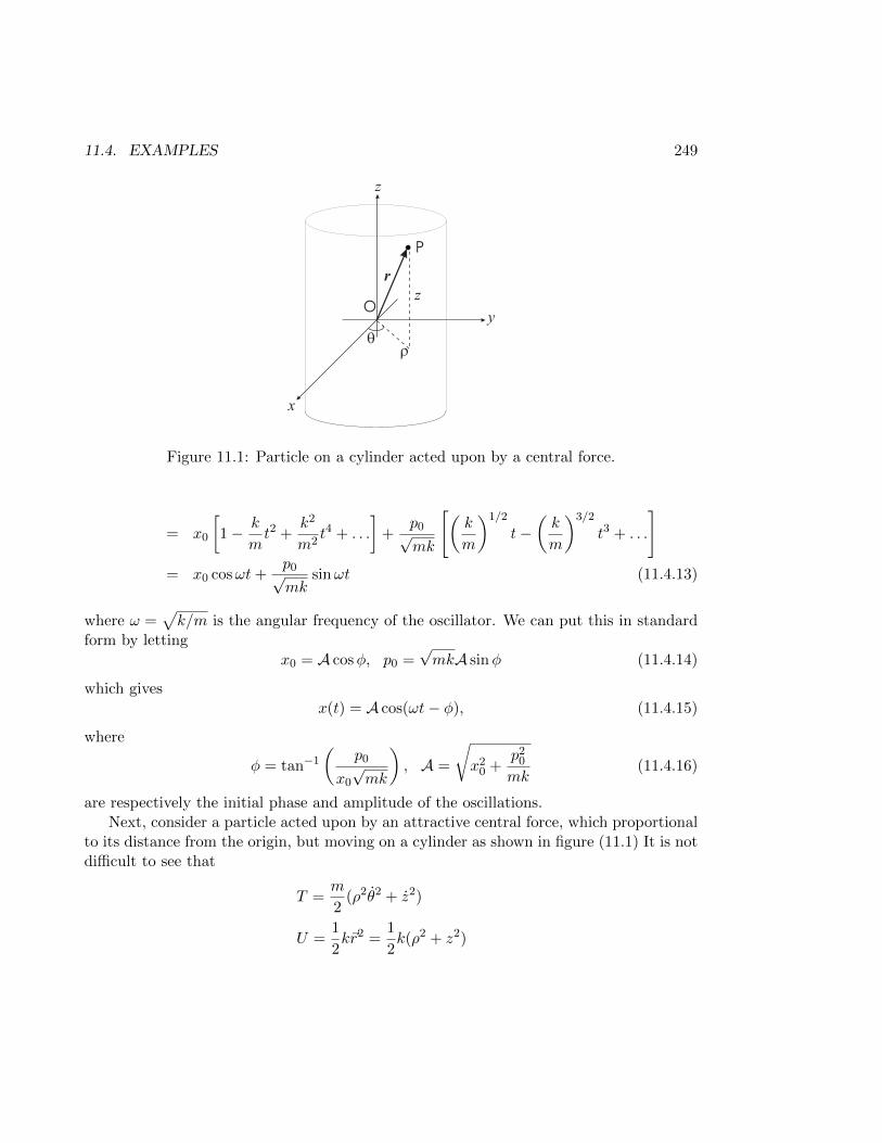
11.4. EXAMPLES 249
r
z
r
P
O
x
y
z
q
Figure 11.1: Particle on a cylinder acted upon by a central force.
= x0
[1− k
mt2 +
k2
m2t4 + . . .
]+
p0√mk
[(k
m
)1/2
t−(k
m
)3/2
t3 + . . .
]= x0 cosωt+
p0√mk
sinωt (11.4.13)
where ω =√k/m is the angular frequency of the oscillator. We can put this in standard
form by lettingx0 = A cosφ, p0 =
√mkA sinφ (11.4.14)
which givesx(t) = A cos(ωt− φ), (11.4.15)
where
φ = tan−1
(p0
x0
√mk
), A =
√x2
0 +p2
0
mk(11.4.16)
are respectively the initial phase and amplitude of the oscillations.Next, consider a particle acted upon by an attractive central force, which proportional
to its distance from the origin, but moving on a cylinder as shown in figure (11.1) It is notdifficult to see that
T =m
2(ρ2θ2 + z2)
U =1
2k~r2 =
1
2k(ρ2 + z2)
250 CHAPTER 11. THE HAMILTONIAN
L =m
2(ρ2θ2 + z2)− k
2(ρ2 + z2) (11.4.17)
and there are no constraints, because they have been solved by using cylindrical coordi-nates and treating ρ as a constant. The Lagrangian equations of motion are
mρ2θ = 0
mz = −kz (11.4.18)
whose solutions are clearly
z = A cos(ωt+ φ), θ = θ0 +Lt
mρ2(11.4.19)
where A and φ are respectively the amplitude and initial phase of an oscillation along the zaxis with angular frequency
√k/m, and L is the angular momentum of the motion around
the cylinder. To compute the Hamiltonian of this system, we determine the generalizedmomenta
pz =∂L∂z
= mz, pθ =∂L∂θ
= mρ2θ, (11.4.20)
invert them to get the velocities as functions of the coordinates and momenta
z =pzm, θ =
pθmρ2
(11.4.21)
and then use (11.1.8) to get the Hamiltonian
H =p2z
2m+
p2θ
2mρ2+k
2(ρ2 + z2) (11.4.22)
(The term kρ2/2 is just a constant which may be discarded by resetting the standard fixedpoint which determines the zero of energy.) The Hamilton equations are
z = z,H =pzm, pz = pz,H = −kz,
θ = θ,H =pθmρ2
, pθ = 0 (11.4.23)
(the last says that pθ is the conserved angular momentum). From our previous example,we recognize the structure of the Poisson brackets for (z, pz) and can write the solutionfor z(t) directly. It is precisely what we had in (11.4.19). To find the solution for θ(t), wenote that
θ = θ,H =1
mρ2pθ,H = 0 (11.4.24)
11.5. THE DIRAC-BERGMANN ALGORITHM FOR SINGULAR SYSTEMS 251
and it follows that all higher derivatives of θ(t) vanish. Therefore, calling pθ = L, thesolution is
θ(t) = θ0 +Lt
mρ2(11.4.25)
as in (11.4.19).3
11.5 The Dirac-Bergmann Algorithm for Singular Systems
So far we have restricted our attention to regular Lagrangian systems. However, byNoether’s theorem we know that this excludes systems with local symmetries and otherconstrained Lagrangian systems . Singular Lagrangian systems are in fact more common(and important) than one may think, although they make their most spectacular appear-ance in field theories as manifestations of local, internal symmetries. In this section weexamine how one can set up the Hamiltonian for singular systems with a finite number ofdegrees of freedom (particle mechanics). The treatment can be extended to systems withan infinite number of degrees of freedom (field theories) and is due to Dirac and Bergman.
What follows is an algorithm, called the Dirac-Bergman algorithm, for constructingthe Hamiltonian of constrained systems. The basic idea is to check, in a systematicfashion, whether or not the equations of motion are consistent. In order to arrive at theHamiltonian we start with the definition of the momenta
pi =∂L∂qi
(11.5.1)
and if the Hessian is invertible then these relations can be solved for the velocities to giveqi = qi(q, p). However, if the Hessian is not invertible then some of the velocities cannotbe expressed in terms of the momenta and it will be possible to solve the equations onlyfor a subset of velocities. Suppose that there are (n− r) of these and that r velocities thatcannot be obtained in terms of the momenta. We will use letters from the beginning of theroman alphabet to label the n − r coordinates whose velocities are expressed in terms ofmomenta and letters from the beginning of the greek alphabet to label the r coordinateswhose velocities cannot be so expressed. From (11.5.1), we will have (n − r) relations ofthe form
qa = fa(qi, pa, qα) (11.5.2)
corresponding to the (n − r) velocities that have been determined in terms of momenta.Inserting these relations into (11.5.1) will give
pi = gi(qi, fa, qα) (11.5.3)
3Problem: Use (11.3.15) to recover the kinematical equations.
252 CHAPTER 11. THE HAMILTONIAN
When i = a the ga are just the momenta pa. The remaining pα cannot depend on the qαbecause, if they did then we could solve for more of the velocities, replacing them withmomenta. Thus we will have r relations of the form
pα = gα(qi, pa) (11.5.4)
These relations will be called the primary constraints. One now defines the canonicalHamiltonian for singular systems by
Hc = piqi − L (11.5.5)
where it is understood that whenever i = a, qa is to be replaced by fa(qi, pa, t) andwhenever i = α, pα is replaced by gα(qi, pa). It is easy to see that Hc is independent of qifor all i, simply because of the definition of the momenta in (11.5.1). Therefore,
Hc = paqa + gαqα − L (11.5.6)
and we have the following derivatives
∂Hc∂qi
=∂gα∂qi
qα −∂L∂qi
∂Hc∂pa
= qa +∂gα∂pa
qα (11.5.7)
These are (2n − r) equations of motion in all.4 Of course, this is a consequence of ther primary constraints in (11.5.4), which restrict the motion to a (2n − r) dimensionalsubspace of the full phase space. For a solution of the Euler-Lagrange equations, pi =∂L/∂qi, i.e.,
pi = −∂Hc∂qi
+∂gα∂qi
qα
qa = +∂Hc∂pa
− ∂gα∂pa
qα (11.5.8)
Our goal is to extend the Hamiltonian to the entire phase space in such a way that thecanonical equations of motion appear the same as they do for canonical systems. To do
4Because Hc cannot depend on the velocities and because the momenta pα can be exchanged in favorof qi and pa, follow the same steps as before with Hc = Hc(qi, pa, )⇒
dHc =∂Hc∂qi
dqi +∂Hc∂pa
dpa +∂Hc∂t
dt
=
(∂gα∂pa
qα + qa
)dpa +
(∂gα∂qi
qα −∂L∂qi
)dqi −
∂L∂t
Comparing the two expressions gives precisely the (2n− r) equations of motion listed.
11.5. THE DIRAC-BERGMANN ALGORITHM FOR SINGULAR SYSTEMS 253
so, we first consider Hc to be a restriction to the desired subspace of another HamiltonianH that is defined on the entire phase space. Now H, being defined on the entire phasespace would be of the form H = H(qi, pi, t) and it cannot be uniquely defined i.e., manyHamiltonians on the entire phase space may have the same restriction,Hc, on the subspace.How then can we construct H?
An arbitrary function on the phase space is called weakly vanishing if it vanishesidentically on a restriction, Γp, of the phase space. One denotes a weakly vanishingfunction, F , by saying that F ≈ 0, i.e.,
F |Γp = 0⇔ F ≈ 0. (11.5.9)
If both F and its gradient vanish on Γp, then F is said to be strongly vanishing, i.e.,
F |Γp = 0
∂F∂qi
∣∣∣Γp
= 0 = ∂F∂pi
∣∣∣Γp
⇔ F ' 0 (11.5.10)
where the symbol ' has been used to denote “strongly” vanishing. Suppose F (qi, pi) is aweakly vanishing function, then
δF |Γp =∂F
∂qiδqi +
∂F
∂piδpi
∣∣∣∣Γp
=∂F
∂qiδqi +
∂F
∂paδpa +
∂F
∂pαδpα
∣∣∣∣Γp
=
(∂F
∂qi+∂F
∂pα
∂gα∂qi
)δqi +
(∂F
∂pa+∂F
∂pα
∂gα∂pa
)δpa (11.5.11)
must also be (weakly) vanishing, which means that
∂F
∂qi+∂F
∂pα
∂gα∂qi≈ 0
∂F
∂pa+∂F
∂pα
∂gα∂pa≈ 0 (11.5.12)
For gα now substitute Gα = pα − gα(qi, pa). Then, ignoring terms that are proportionalto Gα itself (which weakly vanishes), we can rewrite the conditions as
∂
∂qi
(F −Gα
∂F
∂pα
)≈ 0
∂
∂pi
(F −Gα
∂F
∂pα
)≈ 0 (11.5.13)
254 CHAPTER 11. THE HAMILTONIAN
where, in the last equation, we replace the index “a” by “i”, which we can do because
∂Gα∂pβ
= δαβ.
We have proved a useful theorem: if F ≈ 0 then
F −Gα∂F
∂pα' 0. (11.5.14)
We want to apply this idea to the desired Hamiltonian, H(qi, pi).Because H(qi, pi) is required to coincide with Hc on Γp, the function H−Hc ≈ 0 (i.e.,
is weakly vanishing) and therefore
H−Hc −Gα∂H∂pα
' 0. (11.5.15)
because Hc does not depend on pα. It follows that
∂Hc∂qi≈ ∂
∂qi
(H−Gα
∂H∂pα
)def=
∂H∂qi
∂Hc∂pi≈ ∂
∂pi
(H−Gα
∂H∂pα
)def=
∂H∂pi
(11.5.16)
Inserting these into (11.5.8) we find
pi ≈ −∂H∂qi− ∂Gα
∂qiqα ≈ pi, H+ qαGα
qi ≈∂H∂pi
+∂Gα∂pi
qα ≈ qi, H+ qαGα. (11.5.17)
where the brackets are calculated treating the qi and pi as independent, and
H =
(H−Gα
∂H∂pα
)is defined on the entire phase space. The strong equivalence between H and Hc allows usto use Hc instead of H in the equations and we find
pi ≈ pi,Hc + qαGαqi ≈ qi,Hc + qαGα. (11.5.18)
the canonical equations have been returned to their natural form in terms of Poisson brack-ets. They show clearly how Gα, although weakly vanishing , do influence the dynamics.The price we pay is that the equations of motion hold only weakly and the constraintsmust eventually be imposed.
We will now address two issues:
11.5. THE DIRAC-BERGMANN ALGORITHM FOR SINGULAR SYSTEMS 255
• we have assumed that the defining equations are solved so that it is possible toexpress Gα = pα − gα(qi, pa) ≈ 0. In practice this may be a very tedious, if notimpossible task and sometimes it may not even be the desirable thing to do. Is itpossible to carry out the program above if the constraints are to be used instead insome arbitrary form Φα, not necessarily Gα?
• The equations still contain the r undetermined functions qα. We will shortly see thatif constraints in some arbitrary form other than Gα are used then the qα must bereplaced by other functions, ηα (they are the analogues of the Lagrange multipliers):in general, how many of them can be determined?
First, let us rewrite (11.5.18) in terms of arbitrary constraints Φα(qi, pi) ≈ 0, where Gα ≈ 0is a solution. The functional form of Φα is ambiguous since, for example, if Φα ≈ 0then Φ2
α ' 0, so we require that Φα is minimal in the sense that a weakly vanishingfunction should be strongly equivalent to a linear combination of the constraints definingthe constraint surface. Differentiating Φα w.r.t. qi and pa,
∂Φα
∂qi+∂Φα
∂pβ
∂gβ∂qi≈ 0
∂Φα
∂pa+∂Φα
∂pβ
∂gβ∂pa≈ 0 (11.5.19)
The matrix Vαβ = ∂Φα/∂pβ must be non-degenerate, otherwise we could obtain someconstraints involving only q’s, which is impossible. This means that we could express
∂Gβ∂qi
= V −1βα
∂Φα
∂qi∂Gβ∂pa
= V −1βα
∂Φα
∂pa(11.5.20)
Insert these into (11.5.18) to get
pi = pi,Hc − qαV −1αβ
∂Φβ
∂qi
qi = qi,Hc+ qαV−1αβ
∂Φβ
∂pi(11.5.21)
then, with µα = qβV−1βα and the primary Hamiltonian
Hp = Hc + µαΦα, (11.5.22)
we find that the time development of any function, A(qi, pi), on phase space is determinedby
A = A,Hp+∂A
∂t. (11.5.23)
256 CHAPTER 11. THE HAMILTONIAN
The µα play the role of multipliers, as the λl did in the Lagrangian theory. We will nowask how many of them can be determined.
Consistency requires that the constraints should be preserved in time, i.e.,
Φα = Φα,Hp = Φα,Hc+ µβΦα,Φβ ≡ 0 (11.5.24)
Let us call Mαβ = Φα,Φβ and Kα = Φα,Hc then the µα are solutions of the requations
Mαβµβ = −Kα (11.5.25)
and much will depend on the matrix M and the vector Kα.
• Suppose M is non-degenerate and Kα 6= 0, then
µα = M−1αβKβ (11.5.26)
The µα are all fixed and the equations can be solved without ambiguity.
• If M is non-degenerate, but Kα ≡ 0 then there are only the trivial solutions, µα = 0.
• Suppose M is degenerate and Kα 6= 0. If M has rank m < r, then m of the µ’sare determined and the remaining equations determine a certain number, l ≤ r−m,of new relations which are all independent of the previous constraints Φα. If suchnew relations appear, they further constrain the system and are called secondaryconstraints. They restrict the motion to a hypersurface that is of even smallerdimension than the original Γp.
• Finally, if M is degenerate and Kα ≡ 0, non trivial solutions may exist. If m is therank of M then r −m multipliers are weakly fixed.
What is important to bear in mind is that there are situations in which new constraints,the secondary constraints, may emerge. If l new constraints appear, the new constrainthypersurface is the surface defined by the r + l weak relations
Φα ≈ 0, α ∈ 1, ...r
χρ ≈ 0, ρ ∈ 1, ...l (11.5.27)
For consistency, we must now require that the secondary constraints are preserved in time,which implies the new set of relations
χρ,Hc+ µβχρ,Φβ ≈ 0 (11.5.28)
where the weak equality obviously refers to the new hypersurface determined by the r+ lrelations. in (11.5.27). Again, these relations are either fullfilled or lead to new and
11.5. THE DIRAC-BERGMANN ALGORITHM FOR SINGULAR SYSTEMS 257
independent constraints, the tertiary constraints that, together with the primary andsecondary constraints, define a new hypersurface of even lower dimension. In the lattercase, one carries out the iterative procedure again, as before, on this new hypersurface.The process ends after a fininte number of steps. This is the Dirac-Bergman algorithm.
11.5.1 Dirac Bracket
One of the important goals of constrained dynamics is to count the true physical degreesof freedom. Let us distinguish between two kinds of constraints: a constraint, Ψ, is firstclass if it Poisson commutes weakly with all the other constraints
Ψ,Φα ≈ 0 (11.5.29)
otherwise it is second class. Let Υρ denote all second class constraints on a system, then
Cρλ = Υρ,Υλ (11.5.30)
is non-degenerate and we may define a Dirac bracket as follows:
F,G∗ = F,G − F,ΥρC−1ρλ Υλ, G (11.5.31)
The Dirac bracket, satisfies all the conditions of Poisson bractet, viz.,
F,G∗ = −G,F∗
F,GH∗ = F,G∗H +GF,H∗
F, G,H∗∗ + H, F,G∗∗ + G, H,F∗∗ = 0 (11.5.32)
and alsoF,Υα∗ = 0 (11.5.33)
for any F and Υα. Furthermore, the brackets are unchanged if the set Υλ is replacedby any Υ′λ for which the equations Υλ ≈ 0 and Υ′λ ≈ 0 define the same constrainedhypersurface.
We state without proof the following result: if there are n coordinate functions, r firstclass constraints and s second class constraints, the true dynamical degrees of freedom ofthe system are
f = n− r − s
2(11.5.34)
This reflects the fact that two second class constraints are required to eliminate one degreeof freedom. It can be proved that the Dirac bracket is equivalent to the Poisson bracketcalculated using a (reduced) set of unconstrained canonical variables. It is the Diracbracket that gets turned into the commutator upon quantization.
258 CHAPTER 11. THE HAMILTONIAN
11.5.2 Examples
For our first example, let us examine a simple system described by the Lagrangian
L = a(xy − yx)− V (x, y), (11.5.35)
where a is a positive, real constant. The configuration space consists of the coordinates(x, y), but there is no term that is quadratic in the velocities. This does not prevent usfrom writing the Euler-Lagrange equations of motion,
− 2ay +∂V
∂x= 0 = 2ax+
∂V
∂y. (11.5.36)
However, if we compute the momenta,
px =∂L∂x
= −ay, py =∂L∂y
= ax (11.5.37)
we find that they do not contain the velocities and therefore neither x nor y can beeliminated from the Lagrangian. Therefore the two relations above should be thought ofas primary constraints, Φ1 = px + ay ≈ 0 and Φ2 = py − ax ≈ 0. We have the canonicalHamiltonian,
Hc = pxx+ pyy − L = V (x, y) (11.5.38)
and the primary Hamiltonian must be defined with the help of two Lagrange multipliers,µ1 and mu2,
Hp = Hc + µ1(px + ay) + µ2(py − ax) = µ1(px + ay) + µ2(py − ax) + V (x, y). (11.5.39)
The canonical equations of motion will now read read
x = µ1, y = µ2
px = aµ2 −∂V
∂x, py = −aµ1 −
∂V
∂x, (11.5.40)
but consistency of our primary constraints requires that
Φ1 = px + ay = 2aµ2 −∂V
∂x≈ 0 (11.5.41)
and
Φ2 = py − ax = −2aµ1 −∂V
∂y≈ 0. (11.5.42)
11.5. THE DIRAC-BERGMANN ALGORITHM FOR SINGULAR SYSTEMS 259
These are not, however, secondary constraints because they can be solved to determineµ1,2. We find
µ1 ≈ −1
2a
∂V
∂y, µ2 ≈
1
2a
∂V
∂x(11.5.43)
and so we end up with a system of just two primary constraints. The Hamiltonian can berewritten by replacing µ1,2 for their values determined above,
Hp = − 1
2a
∂V
∂y(px + ay) +
1
2a
∂V
∂x(py − ax) + V (x, y) (11.5.44)
The canonical equations are now
x ≈ − 1
2a
∂V
∂y, y ≈ 1
2a
∂V
∂x
px ≈ −1
2
∂V
∂x, py ≈ −
1
2
∂V
∂y(11.5.45)
and the first pair will be recognized as the Euler-Lagrange equations.
The primary constraints are not first class but second class; in fact it is easy to computethe matrix
Cλρ = Φλ,Φρ = 2a
(0 1−1 0
)(11.5.46)
whose inverse appears in the definition of the Dirac bracket between observables. Forinstance, the non-vanishing fundamental Dirac brackets for this system are
x, y∗ = − 1
2a
x, px∗ = y, py∗ =1
2px, py∗ = −a
2(11.5.47)
They are replaced by commutators in Dirac’s quantization scheme. This system had twoconfiguration space variables and two second class constraints, giving it f = 2 − 2/2 = 1degrees of freedom.
Next consider the example of the pendulum described in the previous chapter by theLagrangian
L =m
2(x2 + y2)−mgy + λ(t)(
√x2 + y2 − l) (11.5.48)
The configuration space consists of the three coordinates (x, y, λ). Computing the mo-menta,
px = mx, py = my, pλ = 0, (11.5.49)
260 CHAPTER 11. THE HAMILTONIAN
we see that only λ cannot be determined in terms of momenta. There is one primaryconstraint, i.e., Φ = pλ ≈ 0, so we define the primary Hamiltonian using a multiplier µ
Hp = Hc + µΦλ = pxx+ pyy + µpλ − L
=p2x
2m+
p2y
2m+mgy + µpλ − λ(
√x2 + y2 − l) (11.5.50)
and the canonical equations are
x ≈ pxm
y ≈ pym
λ ≈ µ
px ≈λx√x2 + y2
py ≈ −mg +λy√x2 + y2
pλ ≈√x2 + y2 − l (11.5.51)
The last of course is the consistency condition on the primary constraint. We encounterthe third possibility listed before, the primary constraint pλ ≈ 0 gives rise to secondaryconstraints
χ1 =√x2 + y2 − l ≈ 0
χ2 = xpx + ypy ≈ 0
χ3 =p2x + p2
y
m−mgy + λl ≈ 0 (11.5.52)
andχ3,Hp = χ4 = −3gpy + µl ≈ 0⇒ µ ≈ 3gpy/l. (11.5.53)
when consistency is required order by order according to the Dirac-Bergman algorithm.One can check easily that all the constraints are second class. There are four of them,so the number of dynamical degrees of freedom of this problem is f = 3 − 4/2 = 1. Wealready know that this is the angle made with the vertical (or horizontal) axis.5
5Problem: Evaluate the matrix Cρλ defined earlier and compute the Dirac brackets between pairs ofx, y, λ, px, py, pλ.
11.5. THE DIRAC-BERGMANN ALGORITHM FOR SINGULAR SYSTEMS 261
For a final example, consider the Lagrangian
L =1
2q2
1 + q1q2 + (1− α)q1q2 +β
2(q1 − q2)2 (11.5.54)
The configuration space now consists of the coordinates (q1, q2) and the conjugate momenta
p1 = q1 + q2
p2 = (1− α)q1 (11.5.55)
so q2 cannot be determined in terms of the momenta. The canonical Hamiltonian isdetermined to be
Hc =1
2(p1 − q2)2 − β
2(q1 − q2)2 (11.5.56)
and the second equation in (11.5.55) is a primary constraint, Φ, so we define the primaryHamiltonian
Hp = Hc + µΦ
=1
2(p1 − q2)2 − β
2(q1 − q2)2 + µ[p2 − (1− α)q1] (11.5.57)
giving the canonical equations as
q1 = p1 − q2, q2 = µp1 = β(q1 − q2) + µ(1− α), p2 = (p1 − q2)− β(q1 − q2) (11.5.58)
The primary constraint then leads to the following secondary constraints,
χ1 = α(p1 − q2)− β(q1 − q2) ≈ 0
χ2 = β[(p1 − q2)− α(q1 − q2)] + (α2 − β)µ ≈ 0 (11.5.59)
If α2 = β then it is straightforward to show that all three constraints are first class andµ cannot be determined.6 The system has no degrees of freedom. If α2 6= β then χ2 ≈ 0may be used to determine µ,
µ ≈ β
(β − α2)[(p1 − q2)− α(q1 − q2)] (11.5.60)
and the remaining two constraints have the following Poisson bracket
Φ, χ1P.B = α2 − β (11.5.61)
Consider two special cases:
6Problem: Work out the Poisson algebra of the constraints and show that all the constraints are firstclass if α2 = β.
262 CHAPTER 11. THE HAMILTONIAN
• If α = 0 (β 6= 0) then we find that µ ≈ p1 − q2 and
Hp =1
2(p1 − q2)2 − β
2(q1 − q2)2 + (p1 − q2)(p2 − q1). (11.5.62)
Thus, from the constraints, p2 ≈ q1 and q1 ≈ q2 the equations of motion become
q1 ≈ q2 ≈ p1 ≈ p2 ≈ µ ≈ (p1 − q2) (11.5.63)
in this special case.
• If β = 0 (α 6= 0) then µ = 0 and
Hp =1
2(p1 − q2)2. (11.5.64)
We find the equations of motion q2 ≈ p1 ≈ 0 and
q1 ≈ p2 ≈ p1 − q2 ≈ 0 (11.5.65)
where the last weak equality follows because of the primary constraint.
There are two second class constraints in general and this implies that the system has onedegree of freedom.7
7Problem: Evaluate the matrix Cρλ defined earlier and compute the Dirac brackets between pairs ofq1, q2, p1, p2 for the general case in which α2 6= β.
Chapter 12
Canonical Transformations
Hamilton’s equations do not simplify the problems of mechanics over Euler’s equations. Itis true that Hamilton’s equations are first order, but there are twice as many of them andthey are also coupled differential equations that tend to maintain the same level of difficultyas their second order counterparts. Where then is the new mathematical structure useful?We have already seen that it lends itself particularly to perturbation approaches. Its mainadvantage, however, lies in the fact that it seems to provide a natural framework for theapplication of mechanics in various other areas of physics. For example, it provides thebasis for the formulation of statistical mechanics and quantum mechanics. It also oftenallows for a certain kind of transformation of the fundamental variables of the theory tomore transparent variables (these are the canonical transformations we will discuss in thischapter). Often, new variables can shed new light on a problem and in some cases providethe clues that lead to its solution.
12.1 Hamilton’s equations from a Variational Principle
Let us return to Hamilton’s 2n first order equations governing the dynamics of physicalsystems. In terms of generalized coordinates and momenta, they are
pi = −∂H∂qi
qi =∂H∂pi
. (12.1.1)
Recall that the generalized momenta are defined in terms of the Lagrangian
pi =∂L∂qi
(12.1.2)
263
264 CHAPTER 12. CANONICAL TRANSFORMATIONS
and the Legendre transformation leading from L to H requires the system to be regular,i.e., that the determinant of the Hessian is non-vanishing. The Legendre transformationcan be undone and the Lagrangian expressed as
L = piqi −H(pi, qi) (12.1.3)
where pi are expressed in terms of the velocities. Euler’s equations are then obtained froma variation of the action
S =
∫ 2
1dt[piqi −H(pi, qi)] (12.1.4)
holding the variations of qi(t) fixed at the endpoints. This is sufficient in the Lagrangianformulation.
At this point we may ask if it is possible to use the action in the form (12.1.3), with Lviewed as a function of coordinates and momenta, to directly obtain Hamilton’s equationfrom a variational principle. Because, in Hamilton’s formulation, the momenta are apriori independent of the coordinates (unlike the velocities in Lagrange’s formultion), thecondition that the variations should vanish at the boundary means that we must explicitlyhold both pi and qi fixed there. It is easy to see that we then get
∂L∂pi− d
dt
∂L∂pi
= 0
∂L∂qi− d
dt
∂L∂qi
= 0 (12.1.5)
But, since H contains no time derivatives of the coordinates and momenta, these implypreciesly Hamilon’s equations
qi =∂H∂pi
pi = −∂H∂qi
. (12.1.6)
Note, however, that it appears we have had to pay a price by enlarging the number ofcoordinates whose variations are required to vanish at the boundaries from n to 2n. Thisis not really so because by keeping pi also fixed at the boundaries we avoid a contributionfrom a term of the form
d
dt
(∂L∂pi
δpi
)(12.1.7)
but, because the Lagrangian does not contain derivatives of the momenta, such a termnever appears and holding pi fixed at the end points is redundant. Indeed, a careful lookat the derivation of Euler’s equation reveals that one only needs to get rid of the term
d
dt
(∂L∂qi
δqi
)(12.1.8)
12.2. THE GENERATING FUNCTION 265
so only qi must be held fixed at the boundaries as before.
12.2 The Generating Function
While the canonical equations of motion do not provide a simpler setting for mechanicalproblems than Euler’s equations, they do suggest an alternative approach. To motivatethis approach, let us consider a system system, in which the Lagrangian does not dependon one of the genealized coordinates (say qk), i.e., L = L(q1, . . . , qk, . . . qn, qi, t). Spatialtranslation invariance of the action would then imply that the momentum, pk, conjugateto qk is a constant of the motion, pk = 0. Notice that, in this case, the Hamiltonian is alsoindependent of qk, H = H(q1, . . . , qk, . . . , qn, pi). Coordinates that do not apear explicitlyin the Lagrangian (or Hamiltonian) are called cyclic. If all the coordinates are cyclic thenH = H(pi) and
pi = −∂H∂qi
= 0, qi =∂H∂pi
= ωi (constants) (12.2.1)
(the ωi being functions of only the pi) and it follows that
qi(t) = qi,0 + ωi(t− t0) (12.2.2)
constitutes a complete solution to the problem.This leads us to wonder if there always exists a set of generalized coordinates and mo-
menta that are cyclic. This amounts to turning the observation in the previous paragrapharound to ask if every solution should in fact correspond to precisely such a set. So far wehave considered only coordinate transformations (also known as point transformations),
Qi = Qi(qj , t), (12.2.3)
but the Hamiltonian formulation allows us to consider more general transformations in-volving all of phase space,
qi → Qi = Qi(qj , pj , t)
pi → Pi = Pi(qj , pj , t) (12.2.4)
because it treats the coordinates and momenta on an equal footing, as independent vari-ables.
Not all such transformations will preserve the form of the canonical equations of mo-tion. We therefore define
Canonical Transformations are transformations in phase-space that preserve Hamilton’sequations.
266 CHAPTER 12. CANONICAL TRANSFORMATIONS
To see what the definition implies, let the transformation in (12.2.4) take the Hamiltonianto
H(qi, pi, t)→ K(Qi, Pj , t). (12.2.5)
If it preserves the canoncial equations of motion, we must have
Qi =∂K∂Pi
Pi = − ∂K∂Qi
. (12.2.6)
But because Hamilton’s equations are derivable from an action principle it is sufficient(but not necessary) for both the action
S =
∫ 2
1dt [piqi −H(qi, pi, t)] (12.2.7)
as well as the action
S′ =
∫ 2
1dt[PiQi −K(Qi, Pi, t)
]. (12.2.8)
to be stationary under variations, i.e., δS = 0 = δS′. A sufficient (but again, not neces-sary) condition for this to hold is that
λ[piqi −H(qi, pi, t)] = PiQi −K(Qi, Pi, t) +dF
dt(12.2.9)
where λ is some constant and F = F is any arbitrary function, given either in terms of theold variables or the new. It is called the generating function of the transformation. Ifsome canonical transformations are known then F may be obtained simply by comparingthe two sides of (12.2.9). Viewing F as a function of the qi and pi,
λ[piqi −H] = Pj
[∂Qj∂qi
qi +∂Qj∂pi
pi +∂Qj∂t
]−K +
∂F
∂qiqi +
∂F
∂pipi +
∂F
∂t(12.2.10)
and comparing terms we find
λpi = Pj∂Qj∂qi
+∂F
∂qi
0 = Pj∂Qj∂pi
+∂F
∂pi
λH = K − Pj∂Qj∂t− ∂F
∂t(12.2.11)
12.2. THE GENERATING FUNCTION 267
These are sufficient to determine F (qi, pi, t). However, it is also true that any choice ofF will determine a canonical transformation. It turns out that F is useful only when incan be expressed in special ways in terms of functions depending on half of the variablesfrom the old set and half from the new set. We now consider four particularly usefulpossibilities.
(Type I) F = F1(qi, Qi, t):Suppose that we take the generating function to depend on the old coordinates and thenew coordinates, but not the momenta (old or new). Beginning with (12.2.9), we have
λ[piqi −H] = PiQi −K +∂F1
∂qiqi +
∂F1
∂QiQi +
∂F1
∂t(12.2.12)
which, upon comparison, yields
λpi =∂F1
∂qi
Pi = −∂F1
∂Qi
λH = K − ∂F1
∂t(12.2.13)
These are 2n equations which determine the transformations as follows. The first equa-tion expresses pi in terms of the variables qi, Qi and t. It can be inverted to obtainQi = Qi(qj , pj , t). Once the new coordinates are known functions of the old phase-spacevariables, the second equation gives the new momenta. The last equation returns the newHamiltonian, K (jokingly referred to as the “Kamiltonian”), in terms of the old. Noticethat they are equal up to a scaling and a partial time derivative of F , i.e., they are identicalupto a scale if F has no explicit time dependence.
(Type II) F = F2(qi, Pi, t)− PiQi:If we take a generating function of this form then
λ[piqi −H] = −K − PiQi +∂F2
∂qiqi +
∂F2
∂PiPi +
∂F2
∂t(12.2.14)
gives
λpi =∂F2
∂qi
Qi =∂F2
∂Pi
λH = K − ∂F2
∂t. (12.2.15)
268 CHAPTER 12. CANONICAL TRANSFORMATIONS
They are used to obtain the transformations as follows. The first equation gives pi in termsof qi, Pi and t. It can be inverted to obtain Pi = Pi(qj , pj , t). Once the new momenta areknown as functions of the old phase-space variables, the second equation gives the newcoordinates. As before, the new Hamiltonian is identical to the old upto a scale if F2 isnot explicitly time dependent.
(Type III) F = F3(pi, Qi, t) + λpiqi:For a generating function of this form,
λ[−piqi −H] = −K + PiQi +∂F3
∂pipi +
∂F3
∂QiQi +
∂F3
∂t(12.2.16)
and so
λqi = −∂F3
∂pi
Pi = −∂F3
∂Qi
λH = K − ∂F3
∂t. (12.2.17)
Thus, the first equation allows us to obtain Qi = Qi(qj , pj , t) by inversion and the secondequation then gives Pi = Pi(qj , pj , t). The relationship between H and K is the same asbefore.
(Type IV) F = F4(pi, Pi, t) + λpiqi − PiQi:For a generating function of this form,
λ[−piqi −H] = −K − PiQi +∂F4
∂pipi +
∂F4
∂PiPi +
∂F3
∂t(12.2.18)
and so
λqi = −∂F4
∂pi
Qi =∂F4
∂Pi
λH = K − ∂F4
∂t. (12.2.19)
The first equation allows us to obtain Pi = Pi(qj , pj , t) by inversion, the second then givesQi = Qi(qj , pj , t) and the relationship between H and K is similar to what we had before.
It’s easy to see that invertible coordinate transformations are a particular class ofcanonical transformations generated by a transformation of type II with
F2(qi, Pi, t) = Pifi(qj , t) (12.2.20)
12.3. EXAMPLES 269
and λ = 1. Using the equations appropriate to this case, we see that
pi =∂F2
∂qi= Pj
∂fj∂qi
Qi =∂F2
∂Pi= fj(qi, t) (12.2.21)
Clearly, the transformations of the coordinates must be invertible, i.e., the Jacobian matrixJij = ∂ifj must be invertible. In that case, inverting the first equation gives the newmomenta
Pi = J−1ij (q, t)pj . (12.2.22)
In particular, the transformation generated by
F2(qi, Pi, t) = qiPi (12.2.23)
exchanges is the identity transformation. On the other hand, the following generatingfunction of type I,
F1(qi, Qi, t) = qiQi (12.2.24)
with λ = 1 exchanges coordinates and momenta,
pi =∂F1
∂qi= Qi
Pi = −∂F1
∂Qi= −qi, (12.2.25)
thereby emphasizing the fact that the coordinates and momenta are on an equal footingin the Hamiltonian approach.
12.3 Examples
The Harmonic Oscillator: Consider how a canonical transformation may actually helpsolve a problem by taking the case of a simple harmonic oscillator, whose Hamiltonian isgiven by
H =p2
2m+
1
2mω2q2 (12.3.1)
The fact that the Hamiltonian is a quandratic function of both the coordinates and themomenta suggests a transformation of the form
p = f(P ) cosQ
q =f(P )
mωsinQ (12.3.2)
270 CHAPTER 12. CANONICAL TRANSFORMATIONS
We want to determine f(P ) so that it this is a canonical transformation, therefore let usfind a generating function for it. Eliminating f(P ), we see that
p = mωq cotQ. (12.3.3)
Therefore the generating function must be of type I and, in fact, to recover (12.3.3) wemust have
F1(q,Q, t) =1
2mωq2 cotQ. (12.3.4)
The generating function will now determine f(P ). Using the equations appropriate to atype I generating functional we find
p =∂F1
∂q= mωq cotQ
P = −∂F1
∂Q=
1
2mωq2 csc2Q (12.3.5)
From the first equation one finds that
Q = tan−1 mωq
p, (12.3.6)
and similarly from the second,
P =1
2mω
(p2 +m2ω2q2
). (12.3.7)
Putting (12.3.6) and (12.3.7) together
cosQ =p√
p2 +m2ω2q2=
p√2mωP
sinQ =mωq√
p2 +m2ω2q2=
mωq√2mωP
, (12.3.8)
which may be inverted to get
q =
√2P
mωsinQ
p =√
2mωP cosQ (12.3.9)
Clearly then, f(P ) =√
2mωP . Because F1(q,Q, t) is time independent, the new Hamil-tonian is no different from the original. Re-expressed in terms of the new coordinates wefind
K =1
2m(p2 +m2ω2q2) = ωP (12.3.10)
12.3. EXAMPLES 271
Q is therefore a cyclic coordinate and P is a constant related to the total energy, E, ofthe oscillator. Because Q is cyclic, Q(t) = ωt+Q0 and therefore
q(t) =
√2E
mω2sin(ωt+Q0) (12.3.11)
is the desired solution. While the solution was obvious after the canonical transformation,we must bear in mind that finding the transformation that leads to a maximal number ofcyclic coordinates is generally a difficult problem, which can, as in this case, be a moredifficult enterprise than obtaining a solution of Euler’s (or the canonical) equations for thesystem. Nevertheless it is a novel approach to problem solving.1
Another interesting canonical transformation for the harmonic oscillator is
Q =
√mω
2
(q +
ip
mω
), P = i
√mω
2
(q − ip
mω
)(12.3.12)
To verify that this is a canonical transformation it is only necessary to check the funda-mental Poisson brackets: the only non-vanishing bracket is
Q,P =imω
2
q +
ip
mω, q − ip
mω
= q, p = 1 (12.3.13)
Because the transformation is time independent, the Hamiltonian for the harmonic oscil-lator becomes
K = H = −iωQP (12.3.14)
and the equations of motion read
Q = −iωQ, P = iωP. (12.3.15)
It is now not clear what the Lagrangian system leading to this form of K might corre-spond to because of the impossibility of exchanging the new momentum for a velocity.Nevertheless, we may ask what generating function is responsible for this transformation.Applying the conditions in (12.2.11) we find
∂F
∂q= λp−
√mω
2P =
(λ− 1
2
)p− imωq
2
1The quantization procedure is sadly not invariant under canonical transformations and there can bediffering quantizations of the same system, depending on the phase-space variables chosen. For example,the quantum harmonic oscillator quantized in the (q, p) variables is known to have energy eigenvaluesEn =
(n+ 1
2
)~ω. Consider the time independent Schroedinger’s equation for the same oscillator in the
(Q,P ) system,
Eψ = −i~ω ∂ψ∂Q⇒ ψ = ei
EQ~ω
Because Q is a compact coordinate of period 2π, the wave function is single valued only if En = n~ω forwhole numbers n, since P and therefore E is non-negative. Notice the absence of the vacuum energy 1
2~ω.
272 CHAPTER 12. CANONICAL TRANSFORMATIONS
∂F
∂p= − i√
2mωP =
1
2
(q − ip
mω
)(12.3.16)
Integrating the first equation gives
F =
(λ− 1
2
)pq − imωq2
4+ f(p) (12.3.17)
where f(p) is as yet undetermined. To find an equation for f(p) take a derivative withrespect to p,
∂F
∂p=
(λ− 1
2
)q + f ′(p) (12.3.18)
and compare it with the second of the equations obtained using (12.2.11). They arecompatible if λ = 1 and
f ′(p) = − ip
2mω⇒ f(p) = − ip2
4mω+ const. (12.3.19)
and so
F (q, p) =1
2qp− imωq2
4− ip2
4mω+ const. (12.3.20)
It is not in any of the standard forms given earlier, but can be put in one of them. Forexample, if we want to express the generating functional in terms of F2(q, P ), we couldeliminate p in favor of q and P . But first, recall that
F2(q, P ) = PQ+ F =1
2(qp+QP ) (12.3.21)
Then, by direct substitution we find that
F2(q, P ) =√
2mωqP +i
2(P 2 −mωq2) (12.3.22)
generates the transformation.It has probably become clear that while whether or not a transformation is canonical
has little to do with the physical system, the usefulness of a particular transformationdepends on the particularities of the system. Consider the transformation
Q = ln(1 +√q cos p), P = 2(1 +
√q cos p)
√q sin p (12.3.23)
It is not difficult to show that the only non-vanishing Poisson bracket is Q,P = 1, soit is a canonical transformation. To find a generating function for this transformation wemust solve
λp = P∂Q
∂q+∂F
∂q= sin p cos p+
∂F
∂q
12.3. EXAMPLES 273
0 = P∂Q
∂p+∂F
∂p= −2q sin2 p+
∂F
∂pH = K (12.3.24)
(the last follows because the transformation is time independent). As before, when thesolution of the first,
F (q, p) = λpq − q sin p cos p+ f(p), (12.3.25)
is inserted into the second we get
− 2q sin2 p+ λq − q cos2 p+ q sin2 p+ f ′(p) = (λ− 1)q + f ′(p) = 0 (12.3.26)
which is solved by λ = 1 and f(p) = const. The generating function is
F (q, p) = pq − q sin p cos p (12.3.27)
and we will now express it in terms of F3(p,Q) via
F3(p,Q) = F (q, p)− pq (12.3.28)
where (q, P ) have been eliminated in favor of (p,Q). It is not difficult to see that
q = (eQ − 1)2 sec2 p, P = 2eQ(eQ − 1) tan p (12.3.29)
which givesF3(p,Q) = −(eQ − 1)2 tan p (12.3.30)
from which the transformations in (12.3.29) could be obtained by taking derivatives ap-propriate to the type III generating function.
As a final example, consider the transformation
Q = ln
(1
qsin p
), P = q cot p. (12.3.31)
We may verify that it is a canonical transformation by simply evaluating the fundamentalPoisson brackets. We find that the only non-vanishing bracket is
Q,P =∂Q
∂q
∂P
∂p− ∂Q
∂p
∂P
∂q=
1
q(q csc2 p)− cot2 p ≡ 1 (12.3.32)
so the transformation is canonical. To find a generating function for this transformationwe must solve (12.2.11),
λp = P∂Q
∂q+∂F
∂q= − cot p+
∂F
∂q
274 CHAPTER 12. CANONICAL TRANSFORMATIONS
0 = P∂Q
∂p+∂F
∂p= −q cot2 p+
∂F
∂pH = K (12.3.33)
(the last follows because the transformation is time independent). Integrating the firstequation
F (q, p) = λpq + q cot p+ f(p) (12.3.34)
where f(p) is an arbitrary function of p. Inserting this into the second equation impliesthat
λq − q csc2 p+ f ′(p)− q cot2 p = (λ− 1)q + f ′(p) = 0 (12.3.35)
Evidently, λ = 1 and f(p) = const. solves this equation. Therefore the transformation isgenerated by
F (q, p) = pq + q cot p (12.3.36)
Let us put this in the form F4(q,Q) by eliminating (q,Q) in favor of (p, P ). We find
q = P tan p, Q = ln(cos p
P
)(12.3.37)
which give
F4(p, P ) = F − pq + PQ = P[1 + ln
(cos p
P
)], (12.3.38)
from which (12.3.37) are obtained by taking the derivatives appropriate to generatingfunctions of type IV.
12.4 The Symplectic Approach
If a canonical transformation is independent of time it is called a restricted canonicaltransformation. Let
Pi = Pi(qj , pj), Qi = Qi(qj , pj) (12.4.1)
be a restricted transformation and let K(Q,P ) be the Hamiltonian of the system ex-pressed in terms of the new phase space coordinates. Assume that the transformationsare invertible then
Qi =∂Qi∂qj
qj +∂Qi∂pj
pj (12.4.2)
and therefore
Qi,K =∂Qi∂qjqj ,H+
∂Qi∂pjpj ,H (12.4.3)
or,∂K∂Pi
=∂Qi∂qj
∂H∂pj− ∂Qi∂pj
∂H∂qj
(12.4.4)
12.4. THE SYMPLECTIC APPROACH 275
But, because K ≡ H, we could rewrite the left hand side of the equation to get
∂H∂qj
∂qj∂Pi
+∂H∂pj
∂pj∂Pi
=∂Qi∂qj
∂H∂pj− ∂Qi∂pj
∂H∂qj
(12.4.5)
This shows (by comparing terms) that
∂qj∂Pi
= −∂Qi∂pj
∂pj∂Pi
= +∂Qi∂qj
(12.4.6)
Doing the same things for the second set of canonical equations (for Pi), we get2
∂pj∂Qi
= −∂Pi∂qj
∂qj∂Qi
= +∂Pi∂pj
(12.4.7)
The conditions (12.4.6) and (12.4.7) are called the direct conditions for a restrictedcanonical transformation.
We have shown that the direct conditions are necessary for a transformation to be acanonical transformation, we now show that they are sufficient.3 Suppose that the directconditions hold, then
Qi, Qj =∂Qi∂qk
∂Qj∂pk
− ∂Qi∂pk
∂Qj∂qk
=∂pk∂Pi
∂Qj∂pk
+∂qk∂Pi
∂Qj∂qk
=∂Qj∂Pi
≡ 0 (12.4.8)
where we have used the direct conditions. It is straightforward also that Pi, Pj ≡ 0. Itremains to evaluate
Qi, Pj =∂Qi∂qk
∂Pj∂pk− ∂Qi∂pk
∂Pj∂qk
.
=∂Qi∂qk
∂qk∂Qj
+∂Qi∂pk
∂pk∂Qj
=∂Qi∂Qj
≡ δij (12.4.9)
where use has once again been made of the direct conditions. We have thus proved thata time independent transformation in phase space implies and is implied by the directconditions.
2Problem: Do it!3If a mathematical statement says that condition A implies the condition B (if A then B or A ⇒ B)
then A is “sufficient” for B and B is “necessary” for A. The statement A ⇔ B says that both A and Bare necessary and sufficient for each other: they are identical statements.
276 CHAPTER 12. CANONICAL TRANSFORMATIONS
The restricted transformations can be put in a very elegant and suggestive form if wewrite them out in the language of matrices. Let ~ξ be a “position vector” in phase space,
~ξ = (q1, q2, ...qn, p1, p2, ..., pn) (12.4.10)
Let us think of it as a column matrix and designate an arbitrary component of this vectorby ξα (greek indices), where α ∈ 1, 2, ..., n, n + 1, ..., 2n. Evidently, ξi = qi if i ≤ n andξn+i = pi. Consider the 2n× 2n matrix ω defined by4
ω(2n×2n) =
[0 +1n×n
−1n×n 0
], (12.4.12)
which satisfies the conditions
ω · ω = −12n×2n, ω · ωT = ωT · ω = +12n×2n, (12.4.13)
where
ωT =
[0 −1n×n
+1n×n 0
](12.4.14)
is the transpose of ω. In terms of indices these properties are expressed as
ωαγωγβ = −δαγ (12.4.15)
andωαγωβγ = ωγαωγβ = δαβ. (12.4.16)
Acting on ~ξ,[ω · ~ξ]α = ωαβξβ, (12.4.17)
ω takes qi to pi and pi to −qi, and the direct conditions for a restricted canonical trans-formation take on a simple form when they are written in terms of ω:
∂ηα∂ξβ
= ωαγωβδ∂ξδ∂ηγ
. (12.4.18)
Poisson brackets can be expressed in terms of ω. The fundamental Poisson brackets are
ξα, ξβ = ωαβ (12.4.19)
4It is sometimes more convenient to think of the matrix in terms of its components:
ωαβ =
δαβ β − α = n
−δαβ α− β = n
0 otherwise
. (12.4.11)
12.4. THE SYMPLECTIC APPROACH 277
and, in fact, given any two functions on phase space, A(ξ) and B(ξ), their Poisson brackets
A,B =∂A
∂ξi
∂B
∂ξn+i− ∂A
∂ξn+i
∂B
∂ξi(12.4.20)
may also be expressed as
A,B = ωγδ∂A
∂ξγ
∂B
∂ξδ. (12.4.21)
In particular, suppose we make a time independent transformation ξ → η, then treatingthe new coordinates as functions on phase space and using the above equation it followsthat
ηα, ηβ = ωγδ∂ηα∂ξγ
∂ηβ∂ξδ
(12.4.22)
If the transformation is a restricted canonical transformation, then
ηα, ηβ = = ωγδ∂ηα∂ξγ
∂ηβ∂ξδ
= ωγδωασωγλ∂ξλ∂ησ
∂ηβ∂ξδ
= ωασδδλ∂ξλ∂ησ
∂ηβ∂ξδ
= ωασ∂ξδ∂ησ
∂ηβ∂ξδ
= ωασ∂ηβ∂ησ
= ωασδβσ= ωαβ (12.4.23)
where we have used ω · ωT = 1. It follows that a restricted canonical transformation,ξ → η preserves the form of ω, i.e.,
ωαβ = ωγδ∂ηα∂ξγ
∂ηβ∂ξδ
(12.4.24)
Obviously the converse also holds true because the steps in the above proof are all re-versible.
Let us put the condition in matrix form. Call J the Jacobian matrix,
Jαβ =∂ηα∂ξβ
(12.4.25)
then our necessary (and sufficient, since it is trivial to reverse the above steps) conditionfor the transformation to be canonical is that
ω = J ω JT (12.4.26)
278 CHAPTER 12. CANONICAL TRANSFORMATIONS
where JT is the transpose of J . A restricted canonical transformation preserves ω. In thetheory of continuous groups, the matrix ω is called the symplectic form and transfor-mations that preserve the symplectic form are called symplectic transformations. Re-stricted canonical transformations are therefore symplectic transformations and (12.4.26)is called the symplectic condition. As an example, the transformation
ηα = Jαβξβ (12.4.27)
where ξ = (q, p), η = (Q,P ) and J is a two dimensional rotation matrix, satisfies thesymplectic condition and the transformation is therefore canonical.5
We have thus proved: Restricted Canonical Transformations ⇔ Direct Conditions ⇔Symplectic Condition.
12.5 Infinitesimal Transformations
Let us now focus only infinitesimal canonical transformations,
ξα → ηα(ξ) = ξα + δξα (12.5.1)
i.e.,qi → Qi = qi + δqi, pi → Pi = pi + δpi. (12.5.2)
A suitable generating function for the transformation, which we take for convenience tobe of type II, would be of the form
F2 = qiPi + εG(qi, Pi, t) (12.5.3)
(we are not restricting ourselves to time independent transformations but only to in-finitesimal transformations, and ε is the small parameter of the transformation). Fromthe equations appropriate to type II generating functions, we have
Qi =∂F2
∂Pi= qi + ε
∂G∂Pi
pi =∂F2
∂qi= Pi + ε
∂G∂qi
(12.5.4)
If we restrict ourselves to the first order in ε, then we could replace Pi in G above by pibecause the difference is already of order ε. Then
Qi = qi + ε∂G∂pi
5Problem: Prove this.
12.5. INFINITESIMAL TRANSFORMATIONS 279
Pi = pi − ε∂G∂qi
(12.5.5)
Now we will show that any infinitesimal transformation (not simply a restricted transfor-mation) obeys the symplectic condition. To do so, it’s convenient to return to the notationof the previous section and rewrite these conditions as
ηα = ξα + ε ωαγ∂G∂ξγ
(12.5.6)
The Jacobian matrix of the transformation is then
Jαβ =∂ηα∂ξβ
= δαβ + ε ωαγ∂2G
∂ξβ∂ξγ(12.5.7)
Consider then (upto linear order in ε for consistency)
J ω JT = JαγωγδJTδβ
=
(δαγ + ε ωακ
∂2G∂ξγ∂ξκ
)ωγδ
(δβδ + ε ωβσ
∂2G∂ξδ∂ξσ
)= ωαβ + ε
(ωακωγβ
∂2G∂ξγ∂ξκ
+ ωαδωβσ∂2G
∂ξδ∂ξσ
)+O(ε2)
= ωαβ + ε
(ωακωγβ
∂2G∂ξγ∂ξκ
− ωαδωσβ∂2G
∂ξσ∂ξδ
)+O(ε2)
≈ ωαβ +O(ε2) (12.5.8)
where we have made use of the antisymmetry of ω (i.e., ωβσ = −ωσβ) in the last step. Wehave shown that the symplectic condition is necessary for a general, infinitesimal canonicaltransformation. To show that it is sufficient we begin with the symplectic condition
ωαβ = JαγωγδJTδβ (12.5.9)
and prove that the infinitesimal transformation is canonical. So let
ηα = ξα + ε χα (12.5.10)
and consider ηα, ηβ upto O(ε). We have
ηα, ηβ = ξα + εχα, ξβ + εχβ = ωαβ + ε(ξα, χβ+ χα, ξβ)
= ωαβ + ε
(ωαγ
∂χβ∂ξγ− ωβγ
∂χα∂ξγ
)+O(ε2) (12.5.11)
However, for an infinitesimal transformation of the form (12.5.10),
Jαβ = δαβ + ε∂χα∂ξβ
(12.5.12)
280 CHAPTER 12. CANONICAL TRANSFORMATIONS
so the symplectic condition implies that
ωαβ =
(δαγ + ε
∂χα∂ξγ
)ωγδ
(δβδ + ε
∂χβ∂ξδ
)(12.5.13)
which requires that∂χα∂ξγ
ωγβ + ωαδ∂χβ∂ξδ
= 0 (12.5.14)
or, using the antisymmetry of ω, and relabeling the indices
ωαγ∂χβ∂ξγ− ωβγ
∂χα∂ξγ
= 0 (12.5.15)
It follows that ηα, ηβ = ωαβ i.e., the transformation is canonical.
We have thus proved: General Infinitesimal Canonical Transformations ⇔ SymplecticCondition. It follows that every finite transformation obtained by exponentiating an in-finitesimal canonical transformation (i.e., a finite transformation which is connected tothe identity) is a canonical transformation.
12.6 Hamiltonian as the generator of time translations
We have just seen that an infinitesimal canonical transformation can always be written inthe form
qi → Qi = qi + δqi, δqi = εqi,G
pi → Pi = pi + δpi, δpi = εpi,G (12.6.1)
where G is the generator of the transformation and ε is an infinitesimal parameter. NowG(qi, pi, t) is just about any function of phase space and time. In particular, supposeH(qi, pi, t) is the Hamiltonian and ε = δt, an infinitesimal shift in time. We then have thecanonical transformation
δqi = δtqi,H
δpi = δtpi,H (12.6.2)
These are just the Hamiltonian equations of motion, and we have arrived at an alternativepoint of view: time evolution is just the continuous unfolding of a canonical transfor-mation generated by the Hamiltonian. In other words, the configuration of the system(coordinates and momenta) at any time, t, can be obtained by a series of infinitesimal
12.6. HAMILTONIAN AS THE GENERATOR OF TIME TRANSLATIONS 281
canonical transformations, which is equivalent to a single finite transformation connectedto the identity. Conversely, there is a finite transformation connected to the identity thattakes us from any configuration at t to the initial configuration at t0. This prompts usto seek a canonical transformation to new coordinates, Qi, and momenta, Pi, that areconstants of the motion. This is the subject of the following chapter.
Chapter 13
Hamilton-Jacobi Theory
We have seen that an important objective in studying canonical transformations is thepossible simplification of a mechanical problem. We also ended the last chapter showingthat the Hamiltonian is the generator of time translations and suggested that therefore itmight be possible to find a canonical transformation that takes us from the configurationat any time “t” to the configuration at the initial time, “t0”.This transformation wouldyield Qi = αi, Pi = βi, where αi and βi are the initial conditions that we must in anycase impose upon the system. If it were possible to determine the transformation thenby inversion we would obtain the solution of the problem at any future time. This istantamount to solving the problem so, by conservation of difficulty, we expect that it willbe no easier a task than solving the system by any of the other means already at ourdisposal.
13.1 The Hamilton-Jacobi equation
Suppose that a transformation, generated by F , does precisely what we want then theHamiltonian, H, is transformed into K according to
K = H+∂F∂t. (13.1.1)
But because the new coordinates and momenta are constants of the motion, we must have
Qi =∂K∂Pi
= 0
Pi = − ∂K∂Qi
= 0 (13.1.2)
282
13.1. THE HAMILTON-JACOBI EQUATION 283
which implies that K = K(t) is a function at most of time. Now of course this dependenceon time can be removed by simply defining
F ′ = F −∫K(t)dt (13.1.3)
which does not change the equations of motion, so in all generality we can take K ≡ 0.Now suppose we express F in the form
F = F2(qi, Pi, t)−QiPi (13.1.4)
so that
pi =∂F2
∂qi
Qi =∂F2
∂Pi(13.1.5)
and
K = H(qi,
∂F2
∂qi, t
)+∂F2
∂t≡ 0 (13.1.6)
This can be viewed as an equation for the generating function F2. It is a partial differentialequation in (n + 1) variables, called the “Hamilton-Jacobi” equation. Its solution iscalled “Hamilton’s principal function” and is generally denoted by “S” (we shall useS for F2 from now on). If S can be found we obtain S = S(qi, t), which has no apparentdependence on the new momenta! This is not true, of course, because the integrationinvolves (n+ 1) constants, n of which can be associated with the Pi. Indeed
S = S(qi, βi, βn+1, t) (13.1.7)
What about the last constant, βn+1. How do we know which of the (n + 1) constantsare related to the new momenta? This is easy to resolve because the Hamilton-Jacobiequation involves only derivatives of S,
H(qi,
∂S
∂qi, t
)+∂S
∂t= 0 (13.1.8)
so that S′ = S + β is a solution if S is solution and β is a constant. Thus, one of theconstants, call it βn+1 is additive and we write
S = S(qi, βi, t) + βn+1 (13.1.9)
Of course, βn+1 is completely irrelevant because only derivatives of the generating func-tional are physically meaningful. So we could take
S = S(qi, βi; t) (13.1.10)
284 CHAPTER 13. HAMILTON-JACOBI THEORY
and call βi = Pi. This choice is completely arbitrary. One could just as well choosePi = γi(β1, ...βn) for the momenta and everything that follows would proceed in the sameway. All that is important is that the Pi are constants. Then
Qi =∂S
∂βi(13.1.11)
are the new coordinates. But they too are constants of the motion, so
Qi = αi =∂S
∂βi, (13.1.12)
which equations can be integrated to obtain qi = qi(αi, βi, t).Consider
dS
dt=∂S
∂qiqi +
∂S
∂t(13.1.13)
and note that
pi =∂S
∂qi(13.1.14)
while
H = K − ∂S
∂t= −∂S
∂t(13.1.15)
so
S =
∫dt[piqi −H] + const. (13.1.16)
We have just shown that Hamilton’s principal function differs from the indefinite integralof the Lagrangian by at most a constant. Now the Lagrangian approach is a statementabout the definite integral leading to the Euler-Lagrange equations of motion. Likewise,the Hamilton-Jacobi theory is a statement that the indefinite integral of the Lagrangianleads to the Hamilton-Jacobi equation.
13.2 Two examples
Consider the free particle in one dimension. We choose this example as the simplest, mosttransparent example of the application of the Hamilton-Jacobi equation. Later we’ll workmore complicated examples. The Hamiltonian is just
H =p2
2m(13.2.1)
so the Hamilton Jacobi equation is
1
2m
(∂S
∂q
)2
+∂S
∂t= 0 (13.2.2)
13.2. TWO EXAMPLES 285
and we look for a solution of the form
S = S0(q) + βt. (13.2.3)
Inserting this ansatz into the Hamilton Jacobi equation gives
∂S0
∂q= ±
√2mβ (13.2.4)
so the solution isS(q) = ±
√2mβq − βt+ γ (13.2.5)
where γ is the (irrelevant) additive constant we mentioned before. We associate β withthe new momenta P , and
Q = α =∂S
∂β=
√m
2βq − t (13.2.6)
which can be inverted to give
q =
√2β
m(t+ α) (13.2.7)
Again,
p =∂S
∂q=√
2mβ (13.2.8)
is a constant (the initial momentum p0) and β = p20/2m = E. On the other hand,
q =p0
m(t+ α)⇒ q0 =
√2β
mα⇒ α =
mq0
p0(13.2.9)
Note that β is identified with the total energy of the system.The one dimensional simple Harmonic oscillator provides another transparent example
of the Hamilton-Jacobi approach. In this case,
H =p2
2m+
1
2kq2 (13.2.10)
and the Hamilton-Jacobi equation becomes
1
2m
(∂S
∂q
)2
+1
2mω2q2 +
∂S
∂t= 0 (13.2.11)
Again, seek a solution of the form S = S0(q)− βt so that
dS0
dq= ±
√2mβ
√1− mω2q2
2β(13.2.12)
286 CHAPTER 13. HAMILTON-JACOBI THEORY
and
S0(q) = ±√
2mβ
∫dq
√1− mω2q2
2β+ γ (13.2.13)
where γ is the additive constant we expect. Setting it to zero and soling the integral gives
S(q) =√mβ
[q√2
√1− mω2q2
2β+
√β
mω2sin−1
√mω2
2βq − βt
](13.2.14)
Now P = β and
Q = α =∂S
∂β= −t+
1
ωsin−1
√mω2
2βq (13.2.15)
Therefore
q =
√2β
mω2sin(ωt+ φ) (13.2.16)
where φ = αω. Likewise
p =∂S
∂q=√
2mβ
√1− mω2q2
2β=√
2mβ cos(ωt+ φ) = mq (13.2.17)
Finally, what is the connection between the constants (α, β) and the initial conditions(q0, p0)? we have
q0 =
√2β
mω2sinφ
p0 =√
2mβ cosφ (13.2.18)
Therefore
α =1
ωtan−1 mωq0
p0(13.2.19)
and
β =p2
0
2m+
1
2mω2q2
0 = E (13.2.20)
As before, we see that β is identified with the total energy of the system.
13.3. HAMILTON’S CHARACTERISTIC FUNCTION 287
13.3 Hamilton’s Characteristic Function
In the previous examples we separated Hamilton’s principal function into two parts, thefirst depending only on the coordinates and the second on time. This is always possiblewhen the Hamiltonian is does not explicitly depend on time. To see that this is so, we theprincipal function as
S = W (qi, βi)− βnt (13.3.1)
and plug it into the Hamilton-Jacobi equation to get
H(qi,
∂S
∂qi
)= βn (13.3.2)
which certainly admits time-independent solutions. W (qi, βi, t) is called “Hamilton’sCharacteristic Function” and, moreover, βn is the total energy of the system (recallthat dH/dt = ∂H/∂t ≡ 0). The solution is of the form
W = W (q1, ...qn;β1, ...βn−1)− βn (13.3.3)
and the equations of the canonical transformation are
pi =∂W
∂qi, Qi = αi =
∂W
∂βi− tδi,n. (13.3.4)
We can ascribe a meaning to the characteristic function as well, just as we had for theprincipal function:
dW
dt=∂W
∂qiqi +
∂W
∂t= piqi (13.3.5)
Thus
W =
∫pidqi (13.3.6)
Even though we have yet again reformulated the dynamical problem in terms of a singlenon-linear partial differential equation in n varaibles as opposed to the n ordinary secondorder equations of the Lagrangian theory or the 2n first order equations of the Hamiltoniantheory, the Hamilton-Jacobi theory does not necessarily provide any simplificaton overthe other two approaches. However, in some problems, the Hamilton-Jacobi theory canbe useful and we will now examine two classes of problems in which it can be directlyintegrated.
288 CHAPTER 13. HAMILTON-JACOBI THEORY
13.4 Separability
A coordinate qi is separable if and only if the priciple function can be split into two parts,one depending on qi annd the other depending on all the coordinates except qi, i.e.,
S = S(qi, β1, ...βn; t) + S′(q1, ..., qi, ..., qn, β1, ..., βn; t) (13.4.1)
(where the caret signifies that qi does not appear in S′) and the Hamilton-Jacobi equationalso splits into two parts, one for qi and the other for the remaining coordinates,
Hi(qi,
∂S
∂qi, β1, ..., βn, t
)+∂S
∂t= 0
H′(q1, ..., qi, ...qn,
∂S′
∂qk, ...,
∂S′
∂qn, β1, ..., βn, t
)+∂S′
∂t= 0 (13.4.2)
If all the coordinates are separable then
S =∑i
Si(qi, β1, ..., βn; t) (13.4.3)
where Si dependes only on qi and
H(q1, ..., qn,
∂S
∂q1, ...,
∂S
∂qn, t
)=∑i
Hi(qi,
∂S
∂qi, β1, ...βn; t
)(13.4.4)
When this happens, and if the Hamiltonian does not depend explicityly on time, theproblem can be solved systematically in the following way. Let
Si = Wi(qi, β1, ..., βn−1)− βnt (13.4.5)
then
H(q1, ..., qn,
∂S
∂q1, ...,
∂S
∂q1
)=∑i
βi (13.4.6)
and because H splits according to our assumptions,
Hi(qi,
∂Wi
∂qi, β1, ..., βn
)= βi (13.4.7)
This is a set of uncoupled, ordinary differential equations for the Wi, which can be solvedexactly in principle. The separability of the Hamilton-Jacobi equations is both a propertyof the dynamical system as well as the coordinates in which it is described. No simplecriterion can be given to indicate what coordinate system leads to a separable Hamilton-Jacobi equation for a given system. However, if
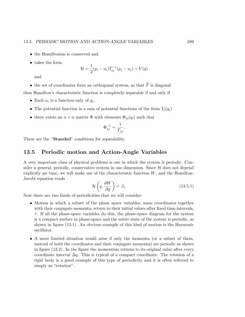
13.5. PERIODIC MOTION AND ACTION-ANGLE VARIABLES 289
• the Hamiltonian is conserved and
• takes the form
H =1
2(pi − ai)T−1
ij (pj − aj) + V (q)
and
• the set of coordinates form an orthogonal system, so that T is diagonal
then Hamilton’s characteristic function is completely separable if and only if
• Each ai is a function only of qi,
• The potential function is a sum of potential functions of the form Vi(qi)
• there exists an n× n matrix Φ with elements Φij(qi) such that
Φ−11j =
1
Tjj.
These are the “Staeckel” conditions for separability.
13.5 Periodic motion and Action-Angle Variables
A very important class of physical problems is one in which the system is periodic. Con-sider a general, periodic, conservative system in one dimension. Since H does not dependexplicitly pn time, we will make use of the characteristic function W , and the Hamilton-Jacobi equation reads
H(q,∂W
∂q
)= β1 (13.5.1)
Now there are two kinds of periodicities that we will consider:
• Motion in which a subset of the phase space variables, some coordinates togetherwith their conjugate momenta, return to their initial values after fixed time intervals,τ . If all the phase-space variables do this, the phase-space diagram for the systemis a compact surface in phase-space and the entire state of the system is periodic, asshown in figure (13.1). An obvious example of this kind of motion is the Harmonicoscillator.
• A more limited situation would arise if only the momenta (or a subset of them,instead of both the coordinates and their conjugate momenta) are periodic as shownin figure (13.2). In the figure the momentum returns to its original value after everycoordinate interval ∆q. This is typical of a compact coordinate. The rotation of arigid body is a good example of this type of periodicity and it is often referred tosimply as “rotation”.
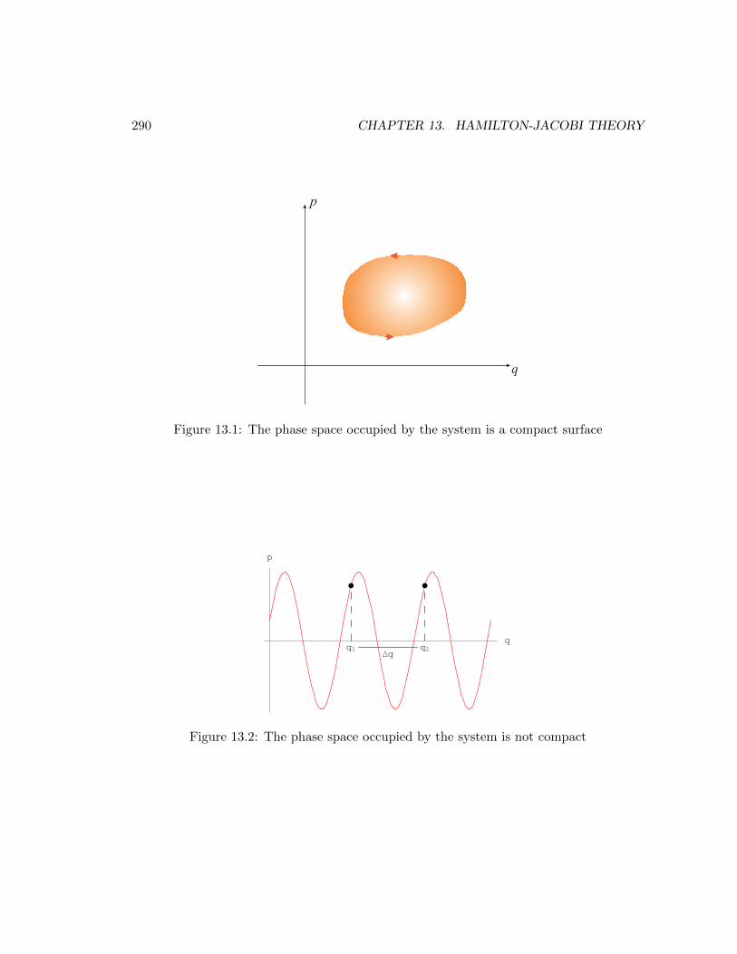
290 CHAPTER 13. HAMILTON-JACOBI THEORY
p
q
Figure 13.1: The phase space occupied by the system is a compact surface
q
p
æ æ
q1 q2Dq
Figure 13.2: The phase space occupied by the system is not compact
13.5. PERIODIC MOTION AND ACTION-ANGLE VARIABLES 291
Both kinds of periodicities can occur in the same system under diffierent initial conditions.For example, take the pendulum. For smaller energies, the motion is periodic in the firstsense. However, if the pendulum’s energy is increased beyond 2mgl, where l is its lengthand m the mass of the bob, then rotational motion will occur.
For either type of motion, introduce the “action” variable
J =
∮pdq (13.5.2)
where the interval is to be carried out over one full period. From the Hamilton-Jacobiequation we determine W = W (q, β1) and
p =∂W
∂q= p(q, β1) (13.5.3)
so we find
J =
∮p(q, β1)dq = J(β1) (13.5.4)
i.e., the variable J depends on β1 alone and the equation can be inverted to give β1 =β1(J). This can be reinserted into W to obtain W as a function of (q, J), i.e., W =W (q, J). Now introduce the “angle” variable
φ(q, J) =∂W
∂J(13.5.5)
and consider the principal function S = W (q, J)−β1(J)t. We find the coordinate conjugateto J
QJ =∂S
∂J= φ− ∂β1
∂Jt (13.5.6)
Now, by construction, QJ ≡ 0, so that
φ =∂β1
∂J= ν(J) (13.5.7)
is constant and depends on J alone. Thus φ = νt+ φ0 and the defining equation (13.5.5)can be inverted to recover q = q(φ, J), which of course is the desired solution.
In and of themselves, the variables φ and J give no particular advantage in solving agiven problem. They do not generally make the problem more tractable. Their merit liesin the physical interpretation that can be given to them. Consider the change in φ as qgoes through a complete period: because
δφ =∂φ
∂qδq (13.5.8)
292 CHAPTER 13. HAMILTON-JACOBI THEORY
(J is a constant of the motion) it follows that over an entire period
∆φ =
∮∂φ
∂qdq =
∮∂2W
∂J∂qdq =
d
dJ
∮∂W
∂qdq ≡ 1 (13.5.9)
This means that ν is the frequency of the motion. Moreover ν is given by
ν =dβ1
dJ=dHdJ
(13.5.10)
so we can determine the frequency of the motion without actually solving the problem, ifit is known a priori that the motion is periodic.
For an example, the Hamilton-Jacobi equation for the one dimensional Harmonic os-cillator,
1
2m
(∂W
∂q
)2
+1
2kq2 = β (13.5.11)
implies that
p =√
2mβ
√1− kq2
2β(13.5.12)
which gives the action variable
J =√
2mβ
∮dq
√1− kq2
2β= 2πβ
√m
k(13.5.13)
Thus
β = H =J
2π
√k
m⇒ ν =
1
2π
√k
m(13.5.14)
To completely solve the problem (i.e., to determine φ(q, J)) we would have to solve theHamilton-Jacobi equation to obtain W (q, J) but, as we see, it is not necessary to do so ifour interest is simply to determine the frequency.
13.6 Further Examples
Consider the simple projectile, described by the Hamiltonian
H =p2x
2m+
p2y
2m+mgy (13.6.1)
where y is the height measured, say, from the surface of the earth. Because the Hamiltonis time independent, choose S = W (x, y) − β2t, then the equation for the characteristicfunction is
1
2m
[(∂W
∂x
)2
+
(∂W
∂y
)2]
+mgy = β2 (13.6.2)
13.6. FURTHER EXAMPLES 293
Let us now see if we can use the separation of variables, writing W = Wx(x) +Wy(y), sothat
1
2m
[(dWx
dx
)2
+
(dWy
dy
)2]
+mgy = β2 (13.6.3)
Therefore,1
2m
(dWy
dy
)2
+mgy = β2 −1
2m
(dWx
dx
)2
= β1 (13.6.4)
because the left hand side depends only on x and the right hand side depends only ony implies that they can only be each equal to a constant. The x equation is directlyintegrated to give
Wx(x) =√
2m(β2 − β1) x+ const. (13.6.5)
The y equation gives
Wy(y) =√
2mβ1
∫dy
√1− mgy
β1= −2
3
√2mβ1
β1
mg
(1− mgy
β1
)3/2
+ const. (13.6.6)
Our separated solution therefore reads
S(x, y, t) =√
2m(β2 − β1) x− 2
3
√2mβ1
β1
mg
(1− mgy
β1
)3/2
− β2t+ γ (13.6.7)
where γ will be recognized as our trivial additive constant. We can now determine x(t)and y(t) of course by simply using the canonical equations
Q1 = α1 =∂S
∂β1
Q2 = α2 =∂S
∂β2(13.6.8)
The second equation gives the solution for x = x(t)
x(t) =
√2
m(β2 − β1)(t+ α2) (13.6.9)
and when this solution is inserted into the first equation, we find after a little algebra that
y(t) =β1
mg
[1− mg2
2β1(t+ α1 + α2)2
]. (13.6.10)
We already know that the constant β2 represents the total energy of the system, so β2 =E = 1
2mv20. To extract the meaning of the constants we must apply some initial conditions:
take~r0 = 0, ~v0 = v0(cos θ, sin θ) (13.6.11)
294 CHAPTER 13. HAMILTON-JACOBI THEORY
then
2(β2 − β1)
mα2
2 = 0
β1
mg
(1− mg2
2β1(α1 + α2)2
)= 0√
2(β2 − β1)
m= v0 cos θ
g(α1 + α2) = −v0 sin θ (13.6.12)
Together, the first and the third imply that α2 = 0. The last gives
α1 = −v0 sin θ
g(13.6.13)
and the second requires that
β1 =1
2mv2
0 sin2 θ (13.6.14)
In fact, with this value of β1, the third equation would then give precisely β2 = E asexpected. Therefore, our solution reads
x(t) = v0 cos θ t
y(t) = v0 sin θ t− 1
2gt2 (13.6.15)
where we get the final answer after inserting the values of the constants above.Our second example is the central force problem discussed at length in a previous
chapter. The Hamiltonian for this problem is
H =1
2m
(p2r +
p2θ
r2+
p2ϕ
r2 sin2 θ
)+ φ(r) (13.6.16)
where φ(r) is the potential energy. As before, we choose S = W (r, θ, ϕ)− β3t so that theequation for the characteristic function becomes
1
2m
[(∂W
∂r
)2
+1
r2
(∂W
∂θ
)2
+1
r2 sin2 θ
(∂W
∂ϕ
)2]
+ φ(r) = β3 (13.6.17)
and we seek separable solutions, i.e., we take W (r, θ, ϕ) = Wr(r) +Wθ(θ) +Wϕ(ϕ). Then(dWr
dr
)2
+1
r2
(dWθ
dθ
)2
+1
r2 sin2 θ
(dWϕ
dϕ
)2
+ 2mφ(r) = 2mβ3 (13.6.18)
13.6. FURTHER EXAMPLES 295
which equation we will separate as follows, writing
r2
[(dWr
dr
)2
+ 2mφ(r)− 2mβ3
]= −
(dWθ
dθ
)2
− 1
sin2 θ
(dWϕ
dϕ
)2
= −β2 (13.6.19)
where we used the fact that the left hand side is a function only of r and the right is afunction only of (θ, φ). Thus we get the radial equation(
dWr
dr
)2
+β2
r2+ 2mφ(r) = 2mβ3 (13.6.20)
The remaining equation can be expressed as(dWϕ
dϕ
)2
= β1(dWθ
dθ
)2
+β1
sin2 θ= β2 (13.6.21)
where β1 is another constant. We will seek a solution that lies wholly in the equatorialplane, i.e., having Wθ =const., θ = π/2 and β1 = β2. Then
Wϕ = ±√β2 φ + const. (13.6.22)
and our radial equation is solved by
Wr = ±√
2m
∫dr
√β3 −
β2
2mr2− φ(r) + const., (13.6.23)
giving Hamilton’s principal function,
S(r, ϕ, t) =√
2m
∫dr
√β3 −
β2
2mr2− φ(r) +
√β2 φ − β3t+ const., (13.6.24)
where we have chosen the positive sign. Thus we find
α3 =∂S
∂β3=
√m
2
∫dr√
β3 − β22mr2
− φ(r)− t
α2 = − 1
2√
2m
∫dr/r2√
β3 − β22mr2
− φ(r)+
ϕ
2√β2
(13.6.25)
If we let α2 = ϕ0/(2√β2), then the second equation above reads√
2m
β2(ϕ− ϕ0) =
∫dr/r2√
β3 − β22mr2
− φ(r)(13.6.26)
296 CHAPTER 13. HAMILTON-JACOBI THEORY
which compares favorably with the second equation in (5.2.24) if β2 is identified with thesquare of the angular momentum, β2 = L2. Furthermore, using the fact that β3 is justthe total energy, E, and rearranging terms we find that the first equation of (13.6.25) is∫
dr√2m [E − V (r)]
= t+ α3 (13.6.27)
where V (r) is the effective potential used in (5.2.17). This is then precisely the firstequation in (5.2.24) and so we have recovered the equations of motion for the central forceproblem.
Chapter 14
Special Relativity
The goal of any relativity theory is to relate measurements performed in one inertial frameof reference to those performed in any other. Galilean relativity is based on the concepts ofan universal or “absolute” space and an “absolute” time, by which is meant that measure-ments of spatial distances and time intervals are observer (or frame) independent providedthat the spatial distances are measured by a simultaneous measurements of the endpoints.Toward the end of the nineteenth century, however, Maxwell’s formulation of electromag-netism, which was completed in 1865, had exposed certain fundamental inconsistenciesbetween the new and extremely successful electromagnetic theory and the Galilean con-ception of space and time. Today we know that Galilean transformations cease to yieldresults that agree with experiment when the relative velocity of the two frames beingcompared is a significant fraction of the speed of light.
In 1887, A. Michelson and E. Morley were able to provide convincing evidence, bymeans of a very clever and now famous experiment named after them, that the speed oflight is the same in all directions and that light does not require a medium in which totravel. At the time their experiment was performed such a medium was assumed to existbecause electromagnetic waves were not considered to be different from other well-knownmechanical waves (eg. sound) and all mechanical waves were known to require a mediumin which to propagate. The putative medium in which light traveled was dubbed theluminiferous aether and was thought to pervade all of space. When wave propagationoccurs in a medium, the frame that is at rest relative to it assumes a special place in thetheory and the “speed” of the wave is its speed as measured in this frame. Thus, thespeed of sound in air at STP is approximately c = 343 m/s in the frame of the air. Aninertial observer moving relative to the medium with velocity ~v in the direction of the wavepropagation or opposite it would observe that the speed of the wave is c∓v, in accordancewith the principles of Galilean relativity. The Michelson and Morley experiment wasdesigned to measure the velocity of the earth relative to the luminiferous aether as it
297
298 CHAPTER 14. SPECIAL RELATIVITY
revolves around the sun during the course of a year. The results were null and the speedof light was found to be the same for propagation in all directions, indicating that theaether was absent. If no such medium exists then the wave speed could be the same forall inertial observers, in other words, a universal constant of nature. This agreed withMaxwell’s theory of electromagnetism, by which electromagnetic waves propagate in avacuum at a speed that depends only on the fundamental constants. Motivated by theMichelson-Morley result and by Maxwell’s theory, A. Einstein recognized in 1905 that thefailure of Galilean relativity at high relative velocities is a consequence of the breakdownof the concepts of “absolute” space and “absolute” time mentioned above. When they areabandoned and replaced by the experimental requirement that the speed of light is thesame in all inertial frames, we arrive at a dramatically new conception of space and timeand therefore of mechanics as well. This modification is known as Einstein’s “special”theory of relativity, or simply Special Relativity and is the topic of this chapter.
We introduce Einstein’s theory in this chapter. We will not dwell much on the questionsand experiments that led up to it, neither shall we concern ourselves too much with theapparent paradoxes (there are many, all of them safely resolved). It is assumed thatthe reader has had some exposure to the topic, so we rather concentrate on the precisemathematical formulation of the theory and on setting up a framework that will be usefulfor the objectives of these notes.
14.1 The Principle of Covariance
It is a general principle that the laws of physics must be the same in all inertial frames. Ifthis were not true, there would be no way to compare the measurements of one (inertial)observer with those of any other.
Mathematically, the fundamental laws of physics would be same in all inertial framesof reference if the equations describing them have the same form in all inertial frames,that is, if the set of transformations that relate one inertial frame to another would, whenapplied to the two sides of any fundamental equation of physics, transform each side inprecisely the same way as the other. This is the principle of covariance and equationsthat have this property are said to be covariant. To further elaborate on this idea,we recall that the transformations that relate two inertial frames will in turn determinethe transformation properties of physical quantities such as velocity, acceleration, etc. Ifthey leave a physical quantity the same in every inertial frame then that quantity is aninvariant or a scalar. Other quantities may not remain invariant but they will transformin a prescribed way. Covariance requires that both sides of the fundamental equationsmust have the same transformation properties. Thus a scalar quantity can only be relatedto another scalar quantity, a vector to a vector and so on.
We will see below that Newton’s laws are covariant under Galilean transformations
14.1. THE PRINCIPLE OF COVARIANCE 299
but Maxwell’s equations are not. This signals an incompatibility between mechanics andelectromagnetism, and incompatibilities always indicate that modifications to one or boththeories are required at a fundamental level. While it is possible that both theories arewrong, it is more fruitful at first to accept one as correct and modify the other so tomake its equations covariant under the transformations that are compatible with the first.Given the fundamental agreement between the predictions of electromagnetism and theexperiment of Michaelson and Morley, Einstein chose the transformations that preserve theform of Maxwell’s equations over the Galilean transformations of Newtonian mechanics.The result is a new formulation of classical mechanics that accounts for the fact that thespeed of light is a finite and a universal constant of nature. In the end, of course, onlyexperiment can decide which theory is correct and, indeed, in the years that followedEinstein’s 1905 paper, it has resoundingly confirmed his choice.
14.1.1 Galilean tranformations
We are familiar with Galilean relativity, which we may conveniently think of as two setsof transformations viz., the “boosts”
~r → ~r′ = ~r − ~vt, t→ t′ = t (14.1.1)
(provided that the frames are coincident at t = 0) and spatial rotations
~r → ~r′ = R ~r, t→ t′ = t (14.1.2)
where R is a rotation matrix (see figure 2). The second of (14.1.1) expresses the abso-luteness of time intervals, as dt′ = dt is the same for all inertial observers. To see thatspatial intervals are also absolute one must remember that the measurement of a distanceinvolves a simultaneous measurement of the endpoints and therefore one has
|d~r′|dt′=0 = |d~r − ~vdt|dt′=dt=0 = |d~r|. (14.1.3)
Consider a single particle within a collection of N particles with interactions betweenthem. If we label the particles by integers, Newton’s equations describing the evolution ofa single particle, say particle n, may be written as,
mnd2~rndt2
= ~F extn + ~F intn = ~F extn +∑m6=n
~F intm→n, (14.1.4)
where ~F intm→n represents the (internal) force that particle m exerts over particle n. Assumethat the external forces are invariant under Galilean boosts, ~F
′extn = ~F extn , and that the
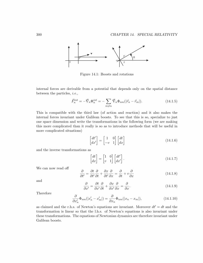
300 CHAPTER 14. SPECIAL RELATIVITY
Figure 14.1: Boosts and rotations
internal forces are derivable from a potential that depends only on the spatial distancebetween the particles, i.e.,
~F intn = −~∇nΦintn = −
∑m 6=n
~∇nΦnm(|~rn − ~rm|). (14.1.5)
This is compatible with the third law (of action and reaction) and it also makes theinternal forces invariant under Galilean boosts. To see that this is so, specialize to justone space dimension and write the transformations in the following form (we are makingthis more complicated than it really is so as to introduce methods that will be useful inmore complicated situations) [
dt′
dx′
]=
[1 0−v 1
] [dtdx
](14.1.6)
and the inverse transformations as[dtdx
]=
[1 0v 1
] [dt′
dx′
]. (14.1.7)
We can now read off∂
∂t′=∂t
∂t′∂
∂t+∂x
∂t′∂
∂x=
∂
∂t+ v
∂
∂x(14.1.8)
and∂
∂x′=
∂t
∂x′∂
∂t+∂x
∂x′∂
∂x=
∂
∂x. (14.1.9)
Therefore∂
∂x′nΦnm(|x′n − x′m|) =
∂
∂xnΦnm(|xn − xm|), (14.1.10)
as claimed and the r.h.s. of Newton’s equations are invariant. Moreover dt′ = dt and thetransformation is linear so that the l.h.s. of Newton’s equations is also invariant underthese transformations. The equations of Newtonian dynamics are therefore invariant underGalilean boosts.
14.1. THE PRINCIPLE OF COVARIANCE 301
14.1.2 Lorentz Transformations
In electrodynamics, on the other hand, in free space one typically ends up with the waveequation,
xψ =1
c2
∂2ψ
∂t2− ~∇2ψ = 0, (14.1.11)
where c is the speed of light in the vacuum and ψ is the “wave function”, which can bethe electromagnetic scalar or vector potential. Now it is an experimental fact that thespeed of light in a vacuum is the same for all inertial observers. However, then (14.1.11) isnot invariant under Galilean transformations. Using the transformations in (14.1.6) and(14.1.7) we have
∂2
∂t′2=
(∂
∂t+ ~v · ~∇
)(∂
∂t+ ~v · ~∇
)(14.1.12)
and~∇′2 = ~∇2. (14.1.13)
Plugging this into the wave equation, we find
1
c2
∂2
∂t′2− ~∇′2 → 1
c2
∂2
∂t2− ~∇2 +
2~v
c2· ~∇ ∂
∂t+
1
c2(~v · ~∇)(~v · ~∇), (14.1.14)
but only the first two terms on the r.h.s. correspond to the wave-equation and, moreover,there is no known kinetic transformation of the wave-function that can return the waveequation to its original form,1 so we must conclude that the electromagnetic wave-equationis not invariant under Galilean transformations. This signals an incompatibility betweenelectromagnetism and Newtonian mechanics therefore, by the principle of covariance, oneof the two must be modified. As we now know, Maxwell’s theory was preferred overNewtonian mechanics, which leads us to ask: what are the transformations that keepMaxwell’s equations covariant? Once we have answered this question we will be in aposition to address the problem of constructing a theory of mechanics that is indeedcovariant under them.
To answer the first question, assume that the transformations that relate two inertialframes continue to be linear (as the Galilean transformations are) and think of the wave-equation as made up of two distinct parts: the second order differential operator, “x”, andthe wave function, ψ, each transforming in its own way under the above transformations.
1Problem: Show that, on the contrary, the Schroedinger equation is invariant under Galilean transfor-mations if they are supplemented with the following kinetic transformation of the wave-function:
ψ → ψ′ = e−i~ (~p·~r−Et)ψ
where ~p = m~v and E = m~v2/2. What does this mean?
302 CHAPTER 14. SPECIAL RELATIVITY
For covariance, we will require “x”, to transform as a scalar (invariant). Let us workwith Cartesian systems and consider some general transformations of the form
t → t′ = t′(t, ~r),
~r → ~r′ = ~r′(t, ~r). (14.1.15)
They must be
1. one-to-one: so that observers may be able to uniquely relate observations, and
2. invertible: so that the transformations can be made from any observer to the other– there is no preferred observer.
Our functions must therefore be bijective. As we have assumed that the transformationsare linear, they will have the form
t′ = − 1
c2(L00t+
∑i
L0ixi),
x′i = Li0t+∑j
Lijxj . (14.1.16)
The reason for this peculiar definition of the coefficents will become clear later. For nowlet us only note that the L’s are some constants that we would like to evaluate. In matrixform the transformations could be written as[
dt′
dx′i
]=
[−L00
c2−L0j
c2
Li0 Lij
] [dtdxj
]. (14.1.17)
The matrix on the r.h.s. is really a 4×4 matrix and Lij represents a 3×3 matrix of purelyspatial transformations. It must be invertible because the transformation is required tobe bijective. For example, L00 = −c2 and L0i = 0 = Li0. The resulting transformationsare purely spatial, transforming xi → x′i =
∑j Lijxj and leaving t → t′ = t unchanged.
Clearly, therefore, the wave-operator,
x → ′x = ∂2t′ − ~∇′2 = ∂2
t − ~∇′2, (14.1.18)
is a scalar if and only if Lij is a spatial rotation, because only then will ~∇′2 = ~∇2.More interesting are the “boosts”, which involve inertial observers with relative ve-
locities. Now Li0 6= 0 6= L0i. Consider relative velocities along the x direction and thetransformation
dt′
dx′1dx′2dx′3
=
α β 0 0γ δ 0 00 0 1 00 0 0 1
dtdx1
dx2
dx3
. (14.1.19)
14.1. THE PRINCIPLE OF COVARIANCE 303
Notice that we have set x′2 = x2 and x′3 = x3. This is because we assumed that spaceis homogeneous and isotropic so that a boost in the x1 direction has no effect on theorthogonal coordinates x2 and x3. We can consider then only the effective two dimensionalmatrix [
dt′
dx′
]=
[α βγ δ
] [dtdx
](14.1.20)
(where x1 := x). Thus we find the inverse transformation[dtdx
]=
1
‖‖
[δ −β−γ α
] [dt′
dx′
], (14.1.21)
where ‖‖ represents the determinant of the transformation, ‖‖ = αδ − βγ and we have
∂
∂t′=
∂t
∂t′∂
∂t+∂x
∂t′∂
∂x=
1
‖‖
(+δ
∂
∂t− γ ∂
∂x
)∂
∂x′=
∂t
∂x′∂
∂t+∂x
∂x′∂
∂x=
1
‖‖
(−β ∂
∂t+ α
∂
∂x
), (14.1.22)
turning our wave-operator into
1
c2
∂2
∂t′2− ~∇′2 =
1
‖‖2
(1
c2
(+δ
∂
∂t− γ ∂
∂x
)2
−(−β ∂
∂t+ α
∂
∂x
)2)
=1
‖‖2
((δ2/c2 − β2)
∂2
∂t2− (α2 − γ2/c2)
∂2
∂x2
−2(αβ − γδ/c2)∂2
∂t∂x
). (14.1.23)
If it is to remain form invariant, the right hand side above has to look the same in theframe S and we need to set
δ2
c2− β2 =
‖‖2
c2,
α2 − γ2
c2= ‖‖2,
αβ − γδ
c2= 0. (14.1.24)
We have four unknowns and three constraints, so there is really just one parameter thatdetermines all the unknowns. It is easy to find. Note that setting
δ = ‖‖ cosh η, β =‖‖c
sinh η (14.1.25)
304 CHAPTER 14. SPECIAL RELATIVITY
solves the first of these equations, as
α = ‖‖ coshω, γ = c‖‖ sinhω (14.1.26)
solves the second. The last equation is then a relationship between η and ω. It impliesthat
sinh η coshω − sinhω coshω = sinh(η − ω) = 0→ η = ω. (14.1.27)
Our boost in the x direction therefore looks like[dt′
dx′
]= ‖‖
[cosh η 1
c sinh ηc sinh η cosh η
] [dtdx
]. (14.1.28)
We notice that ‖‖ is not determined. We will henceforth take it to be unity.What is the meaning of the parameter η? Consider a test body having a velocity u as
observed in the S frame. Its velocity as measured in the S′ frame would be (the velocitydoes not transform as a vector)
u′ =dx′
dt′=
(cosh η)dx+ c(sinh η)dt
(cosh η)dt+ 1c (sinh η)dx
. (14.1.29)
Dividing by (cosh η)dt we find
u′ =u+ c tanh η
1 + uc tanh η
. (14.1.30)
Now suppose that the body is at rest in the frame S. This would mean that u = 0. But,if S′ moves with a velocity v relative to S, we can say that S should move with velocity−v relative to S′. Therefore, because the test body is at rest in S, its velocity relative toS′ should be u′ = −v. Our formula gives
u′ = −v = c tanh η → tanh η = −vc. (14.1.31)
This in turn implies that
cosh η =1√
1− v2/c2, sinh η = − v/c√
1− v2/c2, (14.1.32)
so we can write the transformations in a recognizable form
t′ =t− vx/c2√1− v2/c2
,
x′ =x− vt√1− v2/c2
,
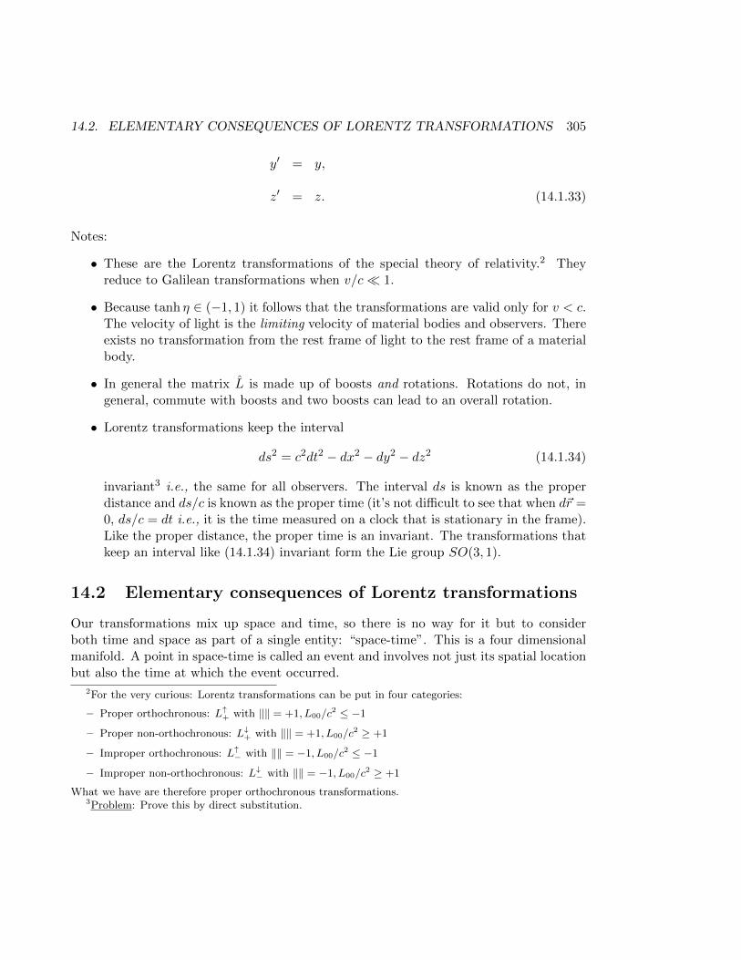
14.2. ELEMENTARY CONSEQUENCES OF LORENTZ TRANSFORMATIONS 305
y′ = y,
z′ = z. (14.1.33)
Notes:
• These are the Lorentz transformations of the special theory of relativity.2 Theyreduce to Galilean transformations when v/c 1.
• Because tanh η ∈ (−1, 1) it follows that the transformations are valid only for v < c.The velocity of light is the limiting velocity of material bodies and observers. Thereexists no transformation from the rest frame of light to the rest frame of a materialbody.
• In general the matrix L is made up of boosts and rotations. Rotations do not, ingeneral, commute with boosts and two boosts can lead to an overall rotation.
• Lorentz transformations keep the interval
ds2 = c2dt2 − dx2 − dy2 − dz2 (14.1.34)
invariant3 i.e., the same for all observers. The interval ds is known as the properdistance and ds/c is known as the proper time (it’s not difficult to see that when d~r =0, ds/c = dt i.e., it is the time measured on a clock that is stationary in the frame).Like the proper distance, the proper time is an invariant. The transformations thatkeep an interval like (14.1.34) invariant form the Lie group SO(3, 1).
14.2 Elementary consequences of Lorentz transformations
Our transformations mix up space and time, so there is no way for it but to considerboth time and space as part of a single entity: “space-time”. This is a four dimensionalmanifold. A point in space-time is called an event and involves not just its spatial locationbut also the time at which the event occurred.
2For the very curious: Lorentz transformations can be put in four categories:
– Proper orthochronous: L↑+ with ‖‖ = +1, L00/c2 ≤ −1
– Proper non-orthochronous: L↓+ with ‖‖ = +1, L00/c2 ≥ +1
– Improper orthochronous: L↑− with ‖‖ = −1, L00/c2 ≤ −1
– Improper non-orthochronous: L↓− with ‖‖ = −1, L00/c2 ≥ +1
What we have are therefore proper orthochronous transformations.3Problem: Prove this by direct substitution.
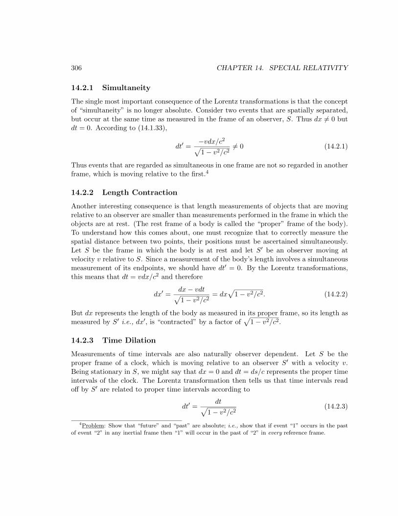
306 CHAPTER 14. SPECIAL RELATIVITY
14.2.1 Simultaneity
The single most important consequence of the Lorentz transformations is that the conceptof “simultaneity” is no longer absolute. Consider two events that are spatially separated,but occur at the same time as measured in the frame of an observer, S. Thus dx 6= 0 butdt = 0. According to (14.1.33),
dt′ =−vdx/c2√1− v2/c2
6= 0 (14.2.1)
Thus events that are regarded as simultaneous in one frame are not so regarded in anotherframe, which is moving relative to the first.4
14.2.2 Length Contraction
Another interesting consequence is that length measurements of objects that are movingrelative to an observer are smaller than measurements performed in the frame in which theobjects are at rest. (The rest frame of a body is called the “proper” frame of the body).To understand how this comes about, one must recognize that to correctly measure thespatial distance between two points, their positions must be ascertained simultaneously.Let S be the frame in which the body is at rest and let S′ be an observer moving atvelocity v relative to S. Since a measurement of the body’s length involves a simultaneousmeasurement of its endpoints, we should have dt′ = 0. By the Lorentz transformations,this means that dt = vdx/c2 and therefore
dx′ =dx− vdt√1− v2/c2
= dx√
1− v2/c2. (14.2.2)
But dx represents the length of the body as measured in its proper frame, so its length asmeasured by S′ i.e., dx′, is “contracted” by a factor of
√1− v2/c2.
14.2.3 Time Dilation
Measurements of time intervals are also naturally observer dependent. Let S be theproper frame of a clock, which is moving relative to an observer S′ with a velocity v.Being stationary in S, we might say that dx = 0 and dt = ds/c represents the proper timeintervals of the clock. The Lorentz transformation then tells us that time intervals readoff by S′ are related to proper time intervals according to
dt′ =dt√
1− v2/c2(14.2.3)
4Problem: Show that “future” and “past” are absolute; i.e., show that if event “1” occurs in the pastof event “2” in any inertial frame then “1” will occur in the past of “2” in every reference frame.
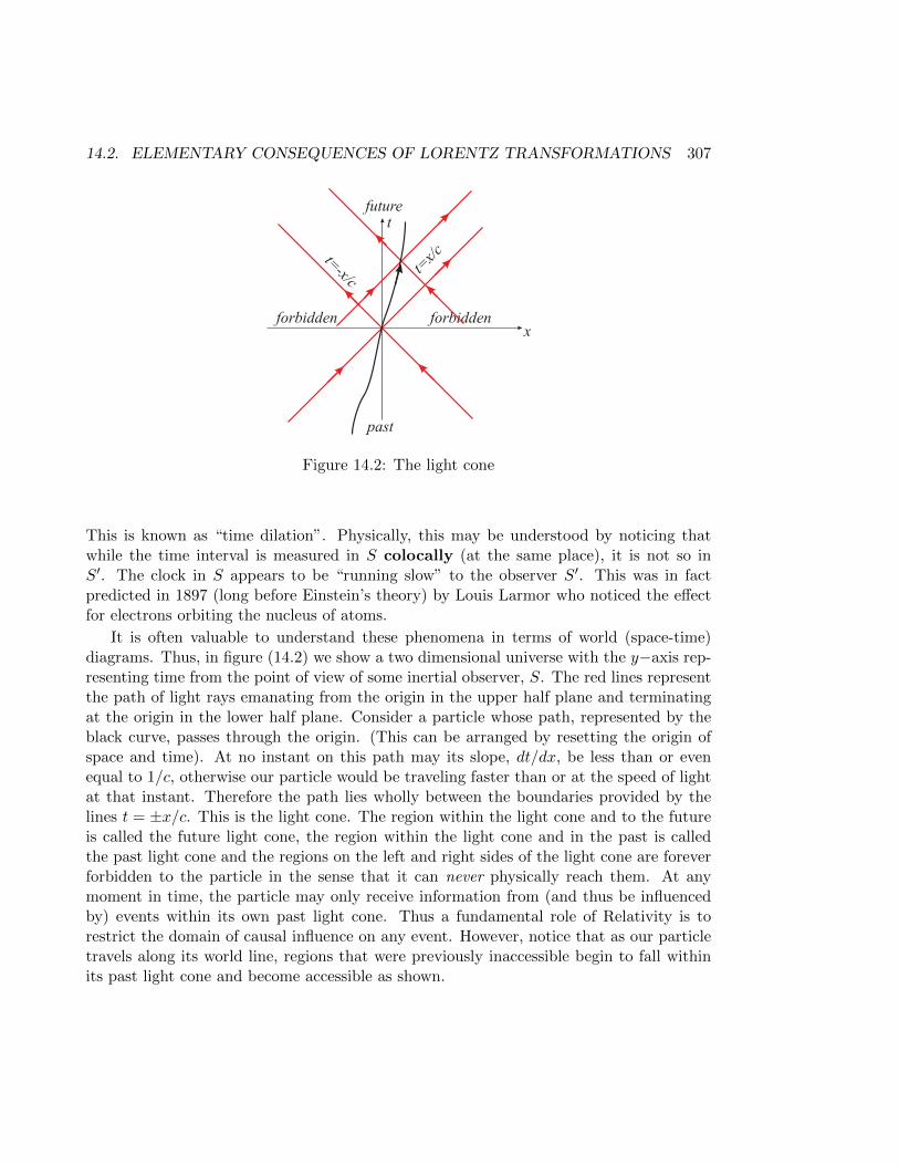
14.2. ELEMENTARY CONSEQUENCES OF LORENTZ TRANSFORMATIONS 307
past
t
x
future
forbidden forbidden
t=x/
ct=-x/c
Figure 14.2: The light cone
This is known as “time dilation”. Physically, this may be understood by noticing thatwhile the time interval is measured in S colocally (at the same place), it is not so inS′. The clock in S appears to be “running slow” to the observer S′. This was in factpredicted in 1897 (long before Einstein’s theory) by Louis Larmor who noticed the effectfor electrons orbiting the nucleus of atoms.
It is often valuable to understand these phenomena in terms of world (space-time)diagrams. Thus, in figure (14.2) we show a two dimensional universe with the y−axis rep-resenting time from the point of view of some inertial observer, S. The red lines representthe path of light rays emanating from the origin in the upper half plane and terminatingat the origin in the lower half plane. Consider a particle whose path, represented by theblack curve, passes through the origin. (This can be arranged by resetting the origin ofspace and time). At no instant on this path may its slope, dt/dx, be less than or evenequal to 1/c, otherwise our particle would be traveling faster than or at the speed of lightat that instant. Therefore the path lies wholly between the boundaries provided by thelines t = ±x/c. This is the light cone. The region within the light cone and to the futureis called the future light cone, the region within the light cone and in the past is calledthe past light cone and the regions on the left and right sides of the light cone are foreverforbidden to the particle in the sense that it can never physically reach them. At anymoment in time, the particle may only receive information from (and thus be influencedby) events within its own past light cone. Thus a fundamental role of Relativity is torestrict the domain of causal influence on any event. However, notice that as our particletravels along its world line, regions that were previously inaccessible begin to fall withinits past light cone and become accessible as shown.
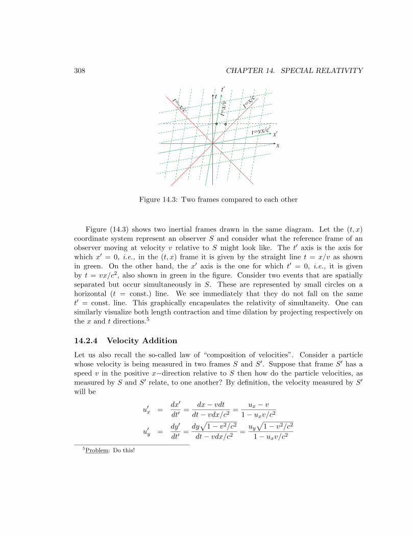
308 CHAPTER 14. SPECIAL RELATIVITY
t
t’
x
x’
t=x/
c
t=x/v
t=vx/c2
t=-x/c
Figure 14.3: Two frames compared to each other
Figure (14.3) shows two inertial frames drawn in the same diagram. Let the (t, x)coordinate system represent an observer S and consider what the reference frame of anobserver moving at velocity v relative to S might look like. The t′ axis is the axis forwhich x′ = 0, i.e., in the (t, x) frame it is given by the straight line t = x/v as shownin green. On the other hand, the x′ axis is the one for which t′ = 0, i.e., it is givenby t = vx/c2, also shown in green in the figure. Consider two events that are spatiallyseparated but occur simultaneously in S. These are represented by small circles on ahorizontal (t = const.) line. We see immediately that they do not fall on the samet′ = const. line. This graphically encapsulates the relativity of simultaneity. One cansimilarly visualize both length contraction and time dilation by projecting respectively onthe x and t directions.5
14.2.4 Velocity Addition
Let us also recall the so-called law of “composition of velocities”. Consider a particlewhose velocity is being measured in two frames S and S′. Suppose that frame S′ has aspeed v in the positive x−direction relative to S then how do the particle velocities, asmeasured by S and S′ relate, to one another? By definition, the velocity measured by S′
will be
u′x =dx′
dt′=
dx− vdtdt− vdx/c2
=ux − v
1− uxv/c2
u′y =dy′
dt′=dy√
1− v2/c2
dt− vdx/c2=uy√
1− v2/c2
1− uxv/c2
5Problem: Do this!
14.3. TENSORS ON THE FLY 309
u′z =dz′
dt′=dz√
1− v2/c2
dt− vdx/c2=uz√
1− v2/c2
1− uxv/c2(14.2.4)
and they all reproduce the Galilean result when c→∞.
14.2.5 Aberration
Finally, we can compare directions in space, as measured by two different observers. Forexample, if the particle is moving in the x−y plane (uz = 0), let us see how two observersmay describe its direction of motion. According to observer S′ the (tangent of the) anglemade with the positive x−axis will be
tan θ′ =u′yu′x
=uy√
1− v2/c2
ux − v=u sin θ
√1− v2/c2
u cos θ − v(14.2.5)
where θ is measured in S and u is the particle speed as measured in S. Notice that itdepends on the speed of the particle as well as the relative speed of the frames. If the“particle” were a photon, i.e., in the case of light propagation, u = c and
tan θ′ =sin θ
√1− v2/c2
cos θ − v/c(14.2.6)
This is the formula for light aberration.6,7
14.3 Tensors on the fly
One lesson that we learn is that we must work with the position vectors of events andthese are “four-vectors”, i.e., vectors having one time and three space components. It isno longer useful or even correct to think of space and time as separate entities becausethe Lorentz transformations mix the two. Continuing with a Cartesian system, label thecoordinates as follows:
xµ = (x0, xi) : µ ∈ 0, 1, 2, 3, x0 = t, xi = xi. (14.3.1)
6Problem: Show that the formula can be simplified to
tanθ′
2= tan
θ
2
√1− v/c1 + v/c
7Problem: Show that for small angles, in the limit v/c→ 0 and up to first order in v/c, the aberrationangle ∆θ = θ − θ′ is given by
∆θ ≈ v
csin θ
310 CHAPTER 14. SPECIAL RELATIVITY
Let us be particular about the position of the indices as superscripts, distinguishing be-tween superscripts and subscripts (soon we will see that this is important) and consider adisplacement, dxµ, in frame S letting the corresponding displacement in frame S′ be dx′µ.By our transformations we know that
dxµ → dx′µ =∑ν
Lµνdxµ, (14.3.2)
where Lµν is precisely the matrix we derived earlier for the special case of boosts in the xdirection. In that case
L00 = −L00/c
2 = cosh η,L0
1 = −L01/c2 = sinh η/c, L0
i = 0 ∀ i ∈ 2, 3,L1
0 = L10 = c sinh η, Li0 = 0 ∀ i ∈ 2, 3,L1
1 = L11 = cosh η, Lij = δij ∀ i, j ∈ 2, 3, (14.3.3)
where δij is the usual Kronecker δ (unit matrix),
δij =
1 i = j0 i 6= j
(14.3.4)
In spacetime, we may set up a vector space V by defining a set of four unit vectors,u(µ), called a tetrad frame, spanning V , so that an arbitrary proper displacement inspace-time can be expressed as d~s =
∑µ dx
µu(µ). Since the displacement itself should notdepend on the observer, it follows from (14.3.2) that under a Lorentz transformation
u(µ) → u′(µ) =∑α
u(α)(L−1)αµ (14.3.5)
A vector is any object of the form ~A =∑
µAµu(µ), with four “contravariant” components,
Aµ, each of which transforms as dxµ (so that ~A is also observer independent), i.e.,
Aµ → A′µ =∑ν
LµνAν . (14.3.6)
It is both customary and useful to think of a vector in terms of its components, but itis somewhat inconvenient to explicitly write out the summation (Σ) every time we havesum over components. We notice, however, that only repeated indices get summed over;therefore we will use Einstein’s convention and drop the symbol Σ, but now with theunderstanding that repeated indices, occurring in pairs in which one member appears“up” (as a superscript) and the other “down” (as a subscript), automatically implies asum. Thus, for example, we would write the above transformation of contravariant vectorsas
Aµ → A′µ = LµνAν . (14.3.7)
14.3. TENSORS ON THE FLY 311
Notice that the derivative operator does not transform as dxµ, but according to the inversetransformation. In other words:
∂
∂xµ:= ∂µ →
∂
∂x′µ:= ∂′µ =
∂xα
∂x′µ∂α. (14.3.8)
But since ∂x′µ/∂xα = Lµα, and
∂xα
∂x′µ∂x′µ
∂xβ= δαβ = (L−1)αµL
µβ, (14.3.9)
it follows that
∂′µ =∂xα
∂x′µ∂α = ∂α(L−1)αµ, (14.3.10)
so the derivatives of a scalar function, ∂µφ(x), are not the components of a vector. Nev-ertheless, we see that
dx′µ∂′µφ′(x′) = (L−1)βµL
µαdx
α∂βφ(x) = δβαdxα∂βφ(x) = dxµ∂µφ(x) (14.3.11)
is invariant.Given any vector space, V , one can one can consider the space of all linear maps from
V to the real numbers, i.e., maps of the form ~ω : V → R,
~ω( ~A)def= ~ω · ~A ∈ R
satisfying~ω(a ~A+ b ~C) = a~ω( ~A) + b~ω(~C) (14.3.12)
where ~A and ~C are in V , and a and a are real numbers. One may now define the sum oftwo linear maps by
(a~ω + b~η)( ~A) = a~ω( ~A) + b~η( ~A) (14.3.13)
then it is easy to see that these maps themselves form a vector space, called the dualvector space, ∗V . Given the tetrad u(µ), spanning V , we could introduce a basis for the
dual vector space, θ(µ), by requiring that
θ(ν)(u(µ)) = θ(ν) · u(µ) = δνµ (14.3.14)
For the inner product to remain invariant, it must hold that, under a Lorentz transforma-tion,
θ(µ) → θ′(µ) = Lµαθ(α). (14.3.15)
Any member of the dual vector space, ~ω can now be expressed as ~ω = ωµθ(µ). ωµ are
called the “covariant” components of ~ω. They will transform as
ωµ → ω′µ = ωα(L−1)αµ, (14.3.16)
312 CHAPTER 14. SPECIAL RELATIVITY
so that, given any vector, ~A, and any dual vector, ~ω, one forms a scalar
− ~ω · ~A = −ωµAµ. (14.3.17)
This is the four dimensional dot product, the analogue of the three dimensional dot productwe are familiar with. The simplest example of a dual vector is the gradient of a scalarfunction:
∇ = θ(µ)∂µφ(x), (14.3.18)
as we saw earlier.We could generalize the concept of vectors to tensors by simply defining a rank (0, n)
tensor to be an multilinear map from a tensor product (an ordered collection) of vectorsto R, i.e., T : V ⊗ V . . . ⊗ V (n times) → R.8 A basis for T will evidently be θ(µ1) ⊗θ(µ2) . . .⊗ θ(µn) and we could express T as
T = Tµ1µ2...µn θ(µ1) ⊗ θ(µ2) . . .⊗ θ(µn), (14.3.19)
Its covariant components will transform as n copies of a dual vector,
T ′µνλ... = Tαβγ...(L−1)αµ(L−1)βν(L−1)γλ . . . (14.3.20)
Similarly, we could define a rank (m, 0) tensor to be an multilinear map from a tensorproduct of dual vectors to R, i.e., T : ∗V ⊗∗V . . .⊗∗V (m times)→ R. Following the samereasoning as before, a basis for T will be u(µ1) ⊗ u(µ2) . . .⊗ u(µm) and we could express Tas
T = Tµ1µ2...µm u(µ1) ⊗ u(µ2) . . .⊗ u(µm) (14.3.21)
so that its contravariant coponents will transform as m copies of a vector,
Tµνλ... = LµαLνβL
λγT
αβγ... (14.3.22)
More generally, we define “mixed” tensors as multilinear maps from a tensor product ofvectors and dual vectors, T : ∗V ⊗ ∗V . . .⊗ ∗V (m times)⊗ V ⊗ V . . .⊗ V (n times)→ Rand express it as
T = Tµν...λκ...u(µ) ⊗ u(ν) . . .⊗ θ(λ) ⊗ θ(κ) . . . , (14.3.23)
with V and ∗V appearing in any order in the product (the above is simply one example).In this case, the tensor is said to have rank (m,n). Thus vectors and dual vectors are butspecial cases of tensors: vectors are tensors of rank (1, 0) and dual vectors are tensors ofrank (0, 1). Just as we think of vectors and dual vectors in terms of their components, wewill also think of tensors in terms of their components. Thus we will speak of contravariant,covariant and mixed tensors according to their components.
8A multilinear map acts lineraly on all its arguments.
14.3. TENSORS ON THE FLY 313
There is a one to one relationship between the covariant and contravariant tensors: forevery covariant tensor we can find a contravariant tensor and vice-versa. To see how thiscomes about, let us rewrite the proper distance (14.1.34) in a slightly different way, usingmatrix notation as follows:
ds2 = −d~s · d~s = −(u(µ) · u(ν))dxµdxν = −ηµνdxµdxν , (14.3.24)
or
u(µ) · u(ν) = ηµν (14.3.25)
where, according to (14.1.34), ηµν is the matrix: diag(−c2, 1, 1, 1) i.e.,
η = ηµν =
−c2 0 0 0
0 1 0 00 0 1 00 0 0 1
. (14.3.26)
It is a covariant tensor of rank two as we see from its transformation properties and iscalled the Minkowski metric. Given that ds2 is invariant, we must have
− ds2 = ηµνdxµdxν → η′αβdx
′αdx′β = η′αβLαµL
βνdx
µdxν = ηµνdxµdxν , (14.3.27)
which implies that
ηµν = LαµLβµη′αβ, (14.3.28)
or, by taking inverses,
η′αβ = (L−1)µα(L−1)νβηµν . (14.3.29)
However, ηµν is required to be an invariant tensor in Special Relativity, η′µν ≡ ηµν , and this
can be used in conjunction with (14.3.28) to derive expressions for the matrices L. It is analternative way of deriving the Lorentz transformations through the so-called generatorsof the transformation (see Appendix B). Now the metric is invertible (‖η‖ 6= 0), withinverse
η−1 = ηµν =
− 1c2
0 0 00 1 0 00 0 1 00 0 0 1
(14.3.30)
and, by construction, ηµαηαν = δµν . (It may be easily shown that the inverse metric ηµν
transforms as
η′αβ = LαµLβνηµν = ηαβ, (14.3.31)
i.e., according the rule for a contravariant tensor of rank two.)
314 CHAPTER 14. SPECIAL RELATIVITY
In (14.3.24), ηµν acts upon two contravariant vectors (two factors of dxµ) to create ascalar, the proper distance between two events. But we had seen that invariants are con-structed from the product of contravariant tensors and covariant tensors. Thus we expectthat ηµνdx
ν should transform as a covariant vector. In general, consider a contravariantvector Aµ and construct the quantity
Aµ = ηµνAν . (14.3.32)
How does it transform? We see that
Aµ → A′µ = ηµνLναA
α = ηµνLναη
αγηγλAλ = (ηµνL
ναη
αγ)(ηγλAλ), (14.3.33)
where we have used ηαγηγλ = δαλ. But notice that (14.3.28) implies the identity
ηαβ = ηµνLµαL
νβ → ηγαηαβ = ηµνη
γαLµαLνβ
→ δγβ = (ηνµLµαη
αγ)Lνβ = (L−1)γνLνβ
→ (L−1)γν = ηνµLµαη
αγ . (14.3.34)
Therefore (14.3.33) readsA′µ = Aγ(L−1)γµ, (14.3.35)
which is the transformation of a covariant vector. The Minkowski metric therefore mapscontravariant vectors to covariant vectors. In the same way it maps contravariant tensorsto covariant tensors:
Tα1,α2,...αn = ηα1β1ηα2β2 ...ηαnβnTβ1,β2,...βn . (14.3.36)
Likewise, the inverse metric ηµν maps covariant vectors to contravariant vectors, i.e., thequantity Aµ defined by
Aµ = ηµνAν , (14.3.37)
transforms as a contravariant vector.9 Therefore, it maps covariant tensors to contravari-ant tensors:
Tα1,α2,...αn = ηα1β1ηα2β2 ...ηαnβnTβ1,β2,...βn . (14.3.38)
This relationship between covariant tensors and contravariant tensors is why we originallydefined the boosts as in (14.1.17). Thus, Lµν = ηµαLαν which gives
L00 = η00L00 = −L00/c
2,
9Problem: Show this!
14.3. TENSORS ON THE FLY 315
L0i = η00L0i = −L0i/c
2,
Li0 = ηijLj0 = Li0,
Lij = ηikLkj = Lij . (14.3.39)
Moreover, there is a natural way to define the (invariant) magnitude of a four-vector, Aµ.It is simply
A2 = −AµAµ = −ηµνAµAν = −ηµνAµAν , (14.3.40)
which is the equivalent of the familiar way of defining the magnitude of an ordinary three-vector.10 For example, the familiar operator x can be written as
x = −ηµν∂µ∂ν = −∂2, (14.3.41)
in which form it is manifestly a scalar. We see once again that the basic difference betweenNewtonian space and Lorentzian space-time is that, in the case of the former, space andtime do not mix and both are absolute. In this case it is sufficient to consider onlyspatial distances and Pythagoras’ theorem ensures that the metric is just the Kronecker δ(with three positive eigenvalues), so there is no need to distinguish between covariant andcontravariant indices. In the case of a Lorentzian space-time an observer’s measurementsof space and time are not independent, neither is absolute and so one is forced to considerthe “distance” between events in space-time. The metric, ηµν , for space-time has signature(−1, 3) i.e., it has one negative eigenvalue and three positive eigenvalues.
For an arbitrary boost specified by a velocity ~v = (v1, v2, v3) = (v1, v2, v3), we find thefollowing Lorentz transformations:
L00 =
1√1− ~v2/c2
= γ,
Li0 = γvi,
L0i =
γvic2,
Lij = δij + (γ − 1)vivj~v2
. (14.3.42)
These are most easily derived using (14.3.28) and the fact that η′µν = ηµν . They reduce tothe transformations we had earlier for a boost in the x− direction, for then ~v = (v, 0, 0)
10When A2 < 0 the vector points within the light cone and is said to be “time-like”. When A2 > 0 itpoints outside the light cone and is called “space-like” and when A2 = 0 the vector A is “light-like” or“null”, pointing along the light cone.
316 CHAPTER 14. SPECIAL RELATIVITY
and
L =
γ −γv
c20 0
−γv γ 0 00 0 1 00 0 0 1
, (14.3.43)
which leads to precisely the transformations in (14.1.33). A more compact way to write(14.3.42) is
t′ = γ[t− (~v · ~r)c2
]
~r′ = ~r − γ~vt+ (γ − 1)~v
v2(~v · ~r) (14.3.44)
for a general ~v.Spatial volume elements are not invariant under Lorentz transformations. We can
make a rough argument for this as follows: suppose that the volume measured by theproper observer is dV then the observer moving relative to this observer with a velocity~v will observe the length dimension in the direction of motion contracted according to(14.2.2) and all perpendicular length dimensions will remain unchanged, so we expectdV ′ = dV/γ. A more precise treatment follows by mimicking the argument for lengthcontraction. Consider the transformation form (t, x)→ (t′x′)
dt′ = L00dt+ L0
jdxj , dx′i = Li0dt+ Lijdx
j (14.3.45)
with dt′ = 0 because length measurements must be made subject to a simultaneous mea-surement of the endpoints in every frame. Therefore dt = −L0
jdxj/γ and
dx′i =
(−1
γLi0L
0j + Lij
)dxj =
(δij +
(1− γ)
γ
vivjv2
)dxj , (14.3.46)
so taking the Jacobian of the transformation gives
d3~r → d3~r′ = d3~r
∣∣∣∣∂x′i∂xj
∣∣∣∣ = d3~r/γ. (14.3.47)
The four dimensional volume element, d4x, is invariant for proper Lorentz transformations.A consequence of the Lorentz transformation of volume is that the three dimensional
δ function, δ(3)(~r − ~r0), which is defined according to∫d3~rδ(3)(~r − ~r0) = 1 (14.3.48)
cannot be invariant either. If we require the defining integral to remain invariant then
δ(3)(~r − ~r0)→ δ′(3)(~r′ − ~r′0) = γδ(3)(~r − ~r0). (14.3.49)
The four dimensional delta function, δ(4)(x− x0), will, however, be invariant.
14.4. WAVES AND THE RELATIVISTIC DOPPLER EFFECT 317
14.4 Waves and the Relativistic Doppler Effect
Maxwell’s equations for the electromagnetic field, Aµ, in Lorentz gauge read
xAµ = jµ. (14.4.1)
In the absence of sources, this is just the wave equation with c being the speed of propa-gation; in one spatial dimension[
∂2
∂t2− c2 ∂
2
∂x2
]Aµ(t, x) = 0 (14.4.2)
and a typical solution will look like a linear combination of plane waves of varying ampli-tudes and frequencies,
A(k)µ (t, x) = A(0)
µ (k, ω)ei(kx−ωt), (14.4.3)
subject to k2−ω2/c2 = 0. Because Aµ transforms as a vector, the exponent must transformas a scalar, i.e., kx − ωt must be an invariant. This is only possible if kµ = (−ω, k)transforms as a covariant vector,
ω′ = γ(ω − vk), k′ = γ(k − vω/c2) (14.4.4)
i.e., kµ = (ω/c2, k) transforms as xµ = (t, x). In particular, the first relation tells us that
f ′ = f
√1− v/c1 + v/c
, (14.4.5)
which is the expression for the Doppler shifting of light in the frame of an observer movingwith a velocity v, taken as positive when the observer is traveling in the direction of thepropagating light wave. Thus an observer moving “away from” the source sees a red-shifting of the light, i.e., a shifting toward lower frequencies, and an observer movingtoward the source sees a blue-shifting, i.e., a shifting toward higher frequencies. Ifthe observer’s speed is small compared to the speed of light, the linear approximation of(14.4.5) gives
f ′ ≈(
1− v
c
)f, (14.4.6)
which should be compared with the Doppler shifting for ordinary mechanical waves thatpropagate in a medium. We get the observed wavelengths either directly, by requiringλf = c = λ′f ′, or by using the second relation in (14.4.4),
λ′ = λ
√1 + v/c
1− v/c. (14.4.7)
318 CHAPTER 14. SPECIAL RELATIVITY
The “redshift” factor is defined as
z =λ′ − λλ
=
√1 + v/c
1− v/c− 1. (14.4.8)
and z ≈ vc when v c. Because all inertial observers are equivalent in special relativity
there is no separate effect for “moving sources” as there is in the case of mechanical waves.Yet, one may wonder why there is an effect at all, considering that light requires no mediumin which to travel and its speed in all reference frames is the same. The Doppler effect forlight originates in time dilation.
14.5 Dynamics in Special Relativity
The relativistic point particle extremizes its “proper time” (this can be thought of as ageneralization of Fermat’s principle, which was originally enunciated for the motion oflight “corpuscles”),
Sp = −mc2
∫dτ = −mc
∫ 2
1
√−ηµνdxµdxν = −mc2
∫ 2
1dt
√1− ~v2
c2(14.5.1)
where dτ = ds/c = 1c
√−ηµνdxµdxν is the proper time and the constant “mc2” is chosen
so that Sp has the dimension of action (or angular momentum: J·s). One sees quite easilythat this action principle reduces to Hamilton’s principle (with zero potential energy,V = 0) when the velocity of the particle relative to the observer is small compared withthe velocity light, for then √
1− ~v2
c2≈ 1− 1
2
~v2
c2(14.5.2)
which, when inserted into (14.5.1) gives
Sp ≈∫ 2
1dt
[1
2m~v2 −mc2
](14.5.3)
The second term is, of course, just a constant (later to be identified with the rest massenergy of the particle) and can be dropped without affecting either the equations of motionor the conservation laws. The first term is the non-relativistic kinetic energy of the particleand the action is therefore just that of a free non-relativistic point particle.
The momentum conjugate to xi is
pi =∂L∂xi
=mvi√
1− ~v2/c2= γmvi, (14.5.4)
14.5. DYNAMICS IN SPECIAL RELATIVITY 319
which reduces to pi = mvi when |~v| << c, and Euler’s equations give
d~p
dt=
d
dt(γm~v) =
d
dt
m~v√1− ~v2/c2
= 0 (14.5.5)
which are the equations of motion of the particle. The Lagrangian does not dependexplicitly on time, so we expect that the Hamiltonian is the total energy and is conserved,
E = H = pixi − L =
m~v2√1− ~v2/c2
+mc2√
1− ~v2/c2 =mc2√
1− ~v2/c2(14.5.6)
The quantity
mR =m√
1− ~v2/c2(14.5.7)
is generally called the “relativistic mass” or simply “mass” of the particle, whereas theparameter m we used initially is called the “rest” mass of the particle and can be thoughtof as its mass when measured in its proper frame (~v = 0). We have just obtained thepopular Einstein relation,
E = mRc2. (14.5.8)
Notice that the energy of the particle is not zero in the rest frame. In this frame theparticle possesses an energy, E = mc2, which is exclusively associated with its proper(rest) mass. Furthermore, expanding E in powers of ~v we find
E = mc2 +1
2m~v2 +
3
8m~v4
c2+ . . . (14.5.9)
The second term is the Newtonian kinetic energy and the higher order terms are allcorrections to the Newtonian expression. The kinetic energy, K, in special relativity isdefined via the relation
E = K +mc2, (14.5.10)
so it is what remains after its rest mass energy is subtracted from its total energy.The Hamiltonian is obtained by a Legendre transformation of the Lagrangian and is
expressed in terms of the momenta and coordinates but not the velocities. This is easilyaccomplished by noting that (14.5.4) gives
~p2 =m2~v2
1− ~v2/c2→ ~v
c=
~p√~p2 +m2c2
(14.5.11)
Thus we get
1− ~v2
c2=
m2c2
~p2 +m2c2, (14.5.12)
320 CHAPTER 14. SPECIAL RELATIVITY
which, when inserted into (14.5.6), gives another well known result,
H = E =√~p2c2 +m2c4. (14.5.13)
Again we recover the rest mass energy, E = mc2 when we set ~p = 0.Let us note that the momentum
pi = mγvi = mdt
dτ
dxidt
= mdxidτ
(14.5.14)
is quite manifestly the spatial component of the four-vector11
pµ = mdxµdτ≡ mUµ. (14.5.15)
where Uµ = dxµ/dτ is the “four velocity” of the particle. The quantity pµ is called its“four momentum”. Its time component is
p0 = −mc2 dt
dτ= − mc2√
1− ~v2/c2= −E (14.5.16)
so we see that the spatial momentum and the energy are components of one four-vectormomentum,
pµ = mdxµ
dτ, p0 =
E
c2, pi =
mvi√1− ~v2/c2
(14.5.17)
Formula (14.5.13) for the energy is now seen to result from a purely kinematic relation,because
p2 = ηµνpµpµ = m2ηµν
dxµ
dτ
dxν
dτ= −m2
[ds
dτ
]2
= −m2c2 (14.5.18)
(the kinematic relation being, of course UµUµ = −c2, remember it). Therefore, expanding
the l.h.s.,
p2 = −E2
c2+ ~p2 = −m2c2, ⇒ E2 = ~p2c2 +m2c4 (14.5.19)
Interestingly, taking the square root allows for both positive and negative energies but wehave chosen the positive sign, thereby excluding negative energy free particles by fiat.
Euler’s equations as given in (14.5.5) are not in a manifestly covariant form. Theycan, however, be put in such a form if we multiply by γ, expressing them as
γd~p
dt=dt
dτ
d~p
dt=d~p
dτ= 0 (14.5.20)
11Problem: Convince yourself that pµ = mdxµ/dτ is indeed a four-vector under Lorentz transformations.Remember that the proper time, τ , is a scalar.
14.5. DYNAMICS IN SPECIAL RELATIVITY 321
This is the equation of motion for a free particle, so the r.h.s. is zero. The l.h.s. transformsas the spatial components of a four-vector and we need not worry about the transforma-tion properties of the r.h.s., since it vanishes. In the presence of an external force ther.h.s. should not vanish and the principle of covariance requires that both sides of theequations of motion should transform in the same way under Lorentz transformations.Let us tentatively write a covariant equation of motion as
dpµ
dτ= fµ (14.5.21)
where fµ is a four-vector. It must be interpreted as the relativistic equivalent of Newton’sforce. If m is constant then
fµ = mdUµ
dτ
and, because U2 = −c2, the “four force” must satisfy one constraint, i.e.,
f · U = fµUµ = 0, (14.5.22)
which means that not all its components are independent. But what is the connectionbetween fµ and the familiar concept of the Newtonian force, which we will call ~FN? Tofind it consider the proper frame, S, of the particle (quantities in this instantaneous restframe will be represented by an over-bar). In this frame τ = t, p0 = m and pi = 0. Itfollows that the time component of the l.h.s of (14.5.21) is zero (assuming m is constant)
and therefore so is f0. The spatial part of the force equation then reads
dpi
dt= mai = f
i, (14.5.23)
where ai is the particle’s acceleration relative to S, generally referred to as its proper ac-
celeration. Naturally, we identify F iN with fi
or, equivalently, with mai. We will discussthe connection between the proper acceleration, ai, and the acceleration as measured inS,
ai =d2xi
dt2
in a later section. For the present take
fµ
= (0, ~FN ). (14.5.24)
To determine fµ in an arbitrary frame we only need to perform a boost because fµ isa genuine four-vector. Therefore, in a frame in which the instantaneous velocity of theparticle is ~v, we find in particular that
f0 = γ~v · ~FNc2
(14.5.25)

322 CHAPTER 14. SPECIAL RELATIVITY
i.e.,dE
dt= ~v · ~FN (14.5.26)
The equation says that the rate of energy gain (loss) of the particle is simply the powertransferred to (or from) the system by the external Newtonian forces. The same boostalso gives the spatial components of the relativistic force in an arbitrary frame as
~f = ~FN + (γ − 1)~v
v2(~v · ~FN ) (14.5.27)
and we notice that the component of ~f perpendicular to the velocity is equal to thecorresponding component of the Newtonian force, ~f⊥ = ~FN⊥. However the component ofthe force in the direction of motion is enhanced over the same component of the Newtonianforce by the factor of γ, i.e., ~f‖ = γ ~FN‖. Our expression also has the non-relativistic limit
(γ ≈ 1) ~f ≈ ~FN , as it should.We have given two forms of the action for the massive point particle in (14.5.1) although
we have concentrated so far on the last of these. The first form is actually quite interesting,
Sp = −mc∫ 2
1
√−ηµνdxµdxν . (14.5.28)
If λ is any parameter describing the particle trajectories then we could write this as
Sp = −mc∫ 2
1dλ√−ηµνUµ(λ)U
ν(λ) (14.5.29)
where
Uµ(λ) =dxµ(λ)
dλ(14.5.30)
is tangent to the trajectories xµ(λ) and λ is an arbitrary parameter. The action is thereforereparameterization invariant and all that we have said earlier corresponds to a particularchoice of λ (= t). This is like fixing a “gauge”, to borrow a term from electrodynamics.12,13
12Problem: Starting from (14.5.28), treat all the coordinates of an event, xµ, on the same footing (insteadof singling out one of them – time – as a parameter) and define
p(λ)µ =∂L∂Uµ(λ)
.
Show thatH = p(λ)µ Uµ(λ) − L = 0.
This is a consequence of reparameterization invariance.13Problem: The square-root Lagrangian in (14.5.28) is inconvenient for the quantization of the free
particle (or working out the statistical mechanics of free, relativistic particles) and a quadratic form,
14.6. CONSERVATION LAWS 323
The relativistic Hamilton-Jacobi equation is obtained by replacing the momenta, pµ,by ∂S/∂xµ in (14.5.19),
ηµν(∂S
∂xµ
)(∂S
∂xν
)= −m2c2 (14.5.31)
We could define S = S′ −mc2t and write the equation in terms of S′,
1
2m(~∇S′)2 −
(∂S′
∂t
)− 1
2mc2
(∂S′
∂t
)2
= 0 (14.5.32)
In this form the limit c → ∞ compares directly with the expected Hamiltonian-Jacobiequation for the free non-relativistic particle.
14.6 Conservation Laws
We will now consider a system of relativistic particles and define the total particle mo-mentum as
pµ =∑n
pµn =∑n
mndxµndτn
=∑n
mnγnvµn (14.6.1)
The rate at which each particle’s four-momentum changes will depend on the net forceacting upon it, according to
dpµndτn
= fµn , (14.6.2)
but this is an inconvenient form of the equation of motion, particularly when dealing withmany particles, because it describes the rate of change with respect to the proper time ofthe particle, which itself depends on its motion. Making use of the fact that γn = dt/dτn,let’s rewrite this equation in the form
dpµndt
= γ−1n fµn (14.6.3)
and therefore alsodpµ
dt=∑n
dpµndt
=∑n
γ−1n fµn . (14.6.4)
similar to the non-relativistic one, is preferable. This can be achieved by introducing an auxiliary function,χ, together with the action,
S = −∫dλ[χηµνU
µ(λ)U
ν(λ) + χ−1m2
]and treating xµ and χ as independent functions with respect to which the action is to be extremized. Showthat one obtains the expected equations of motion.
324 CHAPTER 14. SPECIAL RELATIVITY
Concentrate, for the moment, on the spatial components only and, as before, let ~fn bemade up of two parts, viz., (i) an “external” force, ~f ext
n , acting on the particle and (ii) an“internal” force, ~f int
n acting on it due to its interactions with all the other particles withinthe system. Then
~f intn =
∑m6=n
~fm→n (14.6.5)
and it follows that
d~p
dt=
d
dt
∑n
~pn =∑n,m 6=n
γ−1n~fm→n +
∑n
γ−1n~f extn (14.6.6)
For low particle velocities γn ≈ 1 for all n and ~fn ≈ ~FNn , where ~FN is the Newtonianforce. Conservation of particle momentum in the absence of external forces then followsin this limit by Newton’s third law.
What about the internal forces in a fully relativistic scenario? In principle, no effectexperienced at any world point x can have originated at a world point x′ outside its pastlight cone, i.e., at a time earlier than t−|~r−~r′|/c14 because the speed of light is assumed tobe the maximal speed at which information or influence can travel. Instantaneous particleinteractions, in particular forces that depend only on the spatial distances between theparticles (which are typically employed in Newtonian physics), cannot have the desiredLorentz transformation properties and therefore are impossible in the context of specialrelativity. This, of course, becomes relevant only for very high particle velocities becausethe change in position of one particle can influence another particle only after the infor-mation has had the time to propagate through the distance that separates the particles,which itself changes appreciably during this time if the relative velocities are high, makingthe interactions of particles depend in a complicated way on their motions. This is alreadyevident from the expression
∑n,m 6=n γ
−1n~fm→n describing the effects of the internal forces.
One gets around this difficulty by imagining that the particles are immersed in a set ofdynamical fields whose disturbances propagate in spacetime with a speed not exceedingthe speed of light.
A “field” should be thought of as a potential (or set of potentials) associated witheach point of spacetime. Disturbances in these potentials transfer energy and momentumfrom one event to another. Every field is realized by a function (or set of functions)with definite Lorentz transformation properties and one can have many kinds of fields, eg.scalar fields, vector fields, etc., depending on how the field transforms. Particle-particleinteractions are then described in terms of local interactions of the particles with thefields, which involve an exchange of energy and momentum between the two at the worldpoint of the particle. This exchange causes disturbances in the fields, which then propagate
14This is called retardation.
14.6. CONSERVATION LAWS 325
through spacetime and, at a later time, exchange energy and momentum (locally) withother particles in the system. In this way fields act as mediators of inter-particle forces.A familiar example of this would be electrically charged particles in an electromagneticfield. The electromagnetic field is responsible for energy and momentum transfer betweenthe particles via their electromagnetic interaction.
This picture is only consistent if the field that is responsible for mediating the in-teraction carries energy and momentum in its own right. We then define the total fourmomentum of the system by
Pµ = pµ + πµf (14.6.7)
where πµf represents the field momentum and assert the following:
• In the absence of external forces the total four momentum of the system, whichconsists of the momentum of the particles and the field, is conserved.
This is a natural generalization of the non-relativistic statement about momentum conser-vation and, in fact, follows from Noether’s theorem by space-time translation invariance,as we will see later. It is worth understanding why any generalization of the conservationlaw for momentum must involve the entire four-vector momentum if it is to be a covariantstatement. It can be argued as follows: let ∆E and ∆~P represent the change in energyand momentum respectively of the system in some inertial frame S. In some other frame,S′, we represent these quantities by ∆E′ and ∆~P ′ respectively. Being components of afour vector, they are connected by the Lorentz transformation,
∆P ′i =γvi
c2∆E +
(δij + (γ − 1)
vivjv2
)∆P j
∆E′ = γ(
∆E + ~v ·∆~P). (14.6.8)
It follows that if ∆~P vanishes (the spatial momentum is conserved) in S then it will vanishin S′ if and only if ∆E vanishes as well and if ∆E vanishes (the total energy is conserved)in S then it will vanish in S′ if and only if ∆~P also vanishes. Therefore energy andmomentum conservation go hand in hand in Einstein’s theory of relativity and one cannotbe had without the other. This is a most remarkable fact. In Newtonian mechanics thetwo conservation laws are distinct: momentum conservation requires the absence externalforces and a sufficient condition for the conservation of energy is that all forces acting onthe system are conservative. No such condition appears in the relativistic version of theconservation law, which must therefore always hold provided that the momentum of theparticles and fields are consistently taken into account.
Note that neither the total field momentum nor the total particle momentum is sepa-rately conserved since momentum may be exchanged between the two. This implies that
326 CHAPTER 14. SPECIAL RELATIVITY
the interaction forces between the particles do not satisfy Newton’s third law i.e., actionis not equal and opposite to reaction.
It is often convenient to define the center of momentum frame in complete analogywith the non-relativistic case by setting the spatial components of the total momentum inthat frame to zero, i.e.,
Pµcm =
(Ecm
c2,~0
)= (Mcm,~0), (14.6.9)
which also defines the total rest mass, Mcm, of the system. The rest mass energy, Mcmc2,
contains all the rest energies of the particles that make up the system. It also contains theirkinetic energy relative to the center of mass as well as the energies of their interactionswith one another and of the fields involved in these interactions. In other words, the restmass of the system contains the entire internal energy of the system and it is conserved.We know of four kinds of elementary fields, each with its characteristic interactions. Fromweakest to strongest they are the gravitational field, the fields associated with the weakinteraction, the electromagnetic field and the fields associated with the strong interactionor chromodynamics. The gravitational field is associated with spacetime itself and itsdescription is unique. All the other fields are special cases of a single family of theoriescalled “gauge theories”. These will be discussed in a following chapters. The momentumin a generic frame, S, can be obtained by a Lorentz transformation and will involve onlyMcm and the velocity of the center of mass relative to the Laboratory, ~vcm,
P 0 = Mcmγcm, ~P = Mcmγ~vcm. (14.6.10)
Thus in every physical system consisting of interacting particles, the center of mass willbehave as a single particle with an effective mass (equal to Mcm).
14.7 Relativistic Collisions
The preceding discussion leads directly to the topic of collisions between relativistic par-ticles. In this section we will briefly examine such collisions, assuming that whateverfields are present diminish rapidly enough to zero that the field contribution to the totalmomentum can be ignored when the particles are sufficiently far apart. We will then con-sider “free” incoming particles and “free” outgoing particles as we did earlier and conservemomentum according to
∑n p
µni =
∑n p
µnf as before, but this time taking care with the
relativistic factors.
First consider a collision in which two incoming bodies with momenta
p1i =
(m1 +
K1
c2, ~p1
), p2i =
(m2 +
K2
c2, ~p2
)(14.7.1)
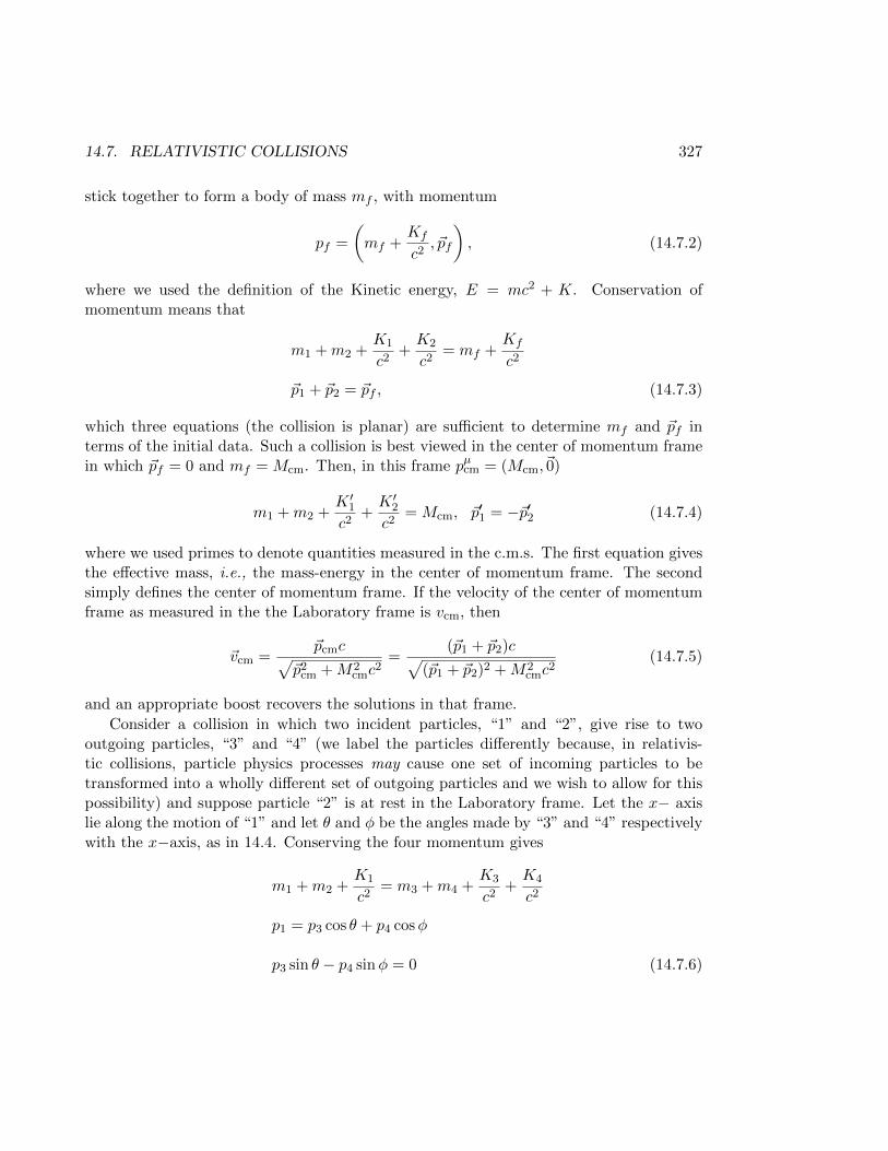
14.7. RELATIVISTIC COLLISIONS 327
stick together to form a body of mass mf , with momentum
pf =
(mf +
Kf
c2, ~pf
), (14.7.2)
where we used the definition of the Kinetic energy, E = mc2 + K. Conservation ofmomentum means that
m1 +m2 +K1
c2+K2
c2= mf +
Kf
c2
~p1 + ~p2 = ~pf , (14.7.3)
which three equations (the collision is planar) are sufficient to determine mf and ~pf interms of the initial data. Such a collision is best viewed in the center of momentum framein which ~pf = 0 and mf = Mcm. Then, in this frame pµcm = (Mcm,~0)
m1 +m2 +K ′1c2
+K ′2c2
= Mcm, ~p′1 = −~p′2 (14.7.4)
where we used primes to denote quantities measured in the c.m.s. The first equation givesthe effective mass, i.e., the mass-energy in the center of momentum frame. The secondsimply defines the center of momentum frame. If the velocity of the center of momentumframe as measured in the the Laboratory frame is vcm, then
~vcm =~pcmc√
~p2cm +M2
cmc2
=(~p1 + ~p2)c√
(~p1 + ~p2)2 +M2cmc
2(14.7.5)
and an appropriate boost recovers the solutions in that frame.
Consider a collision in which two incident particles, “1” and “2”, give rise to twooutgoing particles, “3” and “4” (we label the particles differently because, in relativis-tic collisions, particle physics processes may cause one set of incoming particles to betransformed into a wholly different set of outgoing particles and we wish to allow for thispossibility) and suppose particle “2” is at rest in the Laboratory frame. Let the x− axislie along the motion of “1” and let θ and φ be the angles made by “3” and “4” respectivelywith the x−axis, as in 14.4. Conserving the four momentum gives
m1 +m2 +K1
c2= m3 +m4 +
K3
c2+K4
c2
p1 = p3 cos θ + p4 cosφ
p3 sin θ − p4 sinφ = 0 (14.7.6)
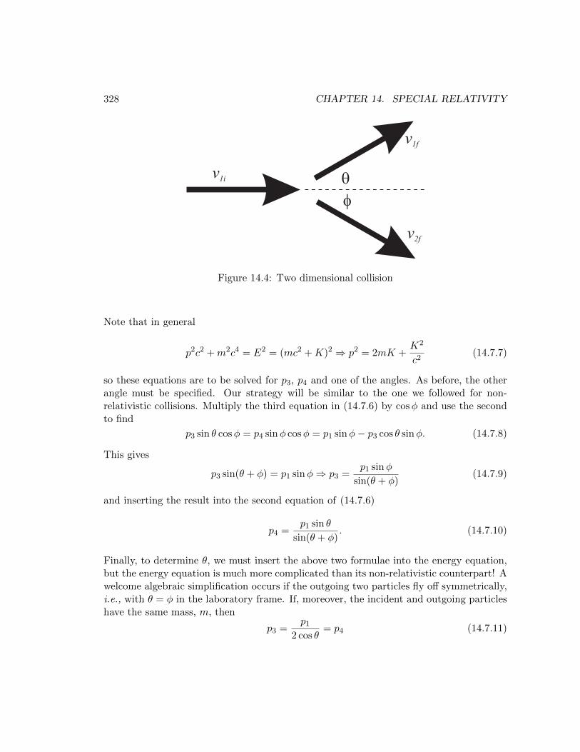
328 CHAPTER 14. SPECIAL RELATIVITY
q
f
v1i
v1f
v2f
Figure 14.4: Two dimensional collision
Note that in general
p2c2 +m2c4 = E2 = (mc2 +K)2 ⇒ p2 = 2mK +K2
c2(14.7.7)
so these equations are to be solved for p3, p4 and one of the angles. As before, the otherangle must be specified. Our strategy will be similar to the one we followed for non-relativistic collisions. Multiply the third equation in (14.7.6) by cosφ and use the secondto find
p3 sin θ cosφ = p4 sinφ cosφ = p1 sinφ− p3 cos θ sinφ. (14.7.8)
This gives
p3 sin(θ + φ) = p1 sinφ⇒ p3 =p1 sinφ
sin(θ + φ)(14.7.9)
and inserting the result into the second equation of (14.7.6)
p4 =p1 sin θ
sin(θ + φ). (14.7.10)
Finally, to determine θ, we must insert the above two formulae into the energy equation,but the energy equation is much more complicated than its non-relativistic counterpart! Awelcome algebraic simplification occurs if the outgoing two particles fly off symmetrically,i.e., with θ = φ in the laboratory frame. If, moreover, the incident and outgoing particleshave the same mass, m, then
p3 =p1
2 cos θ= p4 (14.7.11)
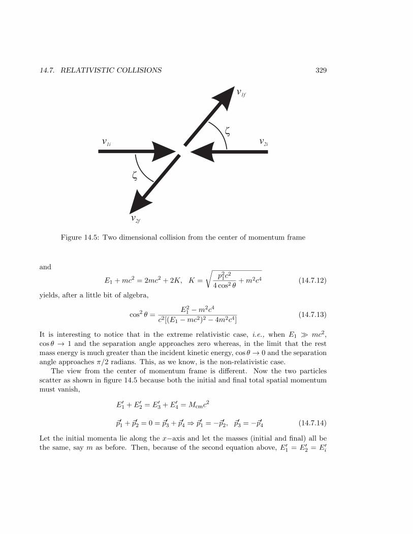
14.7. RELATIVISTIC COLLISIONS 329
z
z
v1i v2i
v1f
v2f
Figure 14.5: Two dimensional collision from the center of momentum frame
and
E1 +mc2 = 2mc2 + 2K, K =
√p2
1c2
4 cos2 θ+m2c4 (14.7.12)
yields, after a little bit of algebra,
cos2 θ =E2
1 −m2c4
c2[(E1 −mc2)2 − 4m2c4](14.7.13)
It is interesting to notice that in the extreme relativistic case, i.e., when E1 mc2,cos θ → 1 and the separation angle approaches zero whereas, in the limit that the restmass energy is much greater than the incident kinetic energy, cos θ → 0 and the separationangle approaches π/2 radians. This, as we know, is the non-relativistic case.
The view from the center of momentum frame is different. Now the two particlesscatter as shown in figure 14.5 because both the initial and final total spatial momentummust vanish,
E′1 + E′2 = E′3 + E′4 = Mcmc2
~p′1 + ~p′2 = 0 = ~p′3 + ~p′4 ⇒ ~p′1 = −~p′2, ~p′3 = −~p′4 (14.7.14)
Let the initial momenta lie along the x−axis and let the masses (initial and final) all bethe same, say m as before. Then, because of the second equation above, E′1 = E′2 = E′i
330 CHAPTER 14. SPECIAL RELATIVITY
and E′3 = E′4 = E′f and because of energy conservation 2E′i = 2E′f = Mcmc2. Therefore
all momenta have the same magnitude. Since the final velocities are anti-parallel, thereis only one final angle, ξ, between the outgoing particles and the x−axis, but there isnot enough information to determine it. However, we can relate ξ to the angle θ in theLaboratory frame discussed earlier by performing a Lorentz transformation.15
In general, a good amount of information about any collision in any frame is obtaineddirectly from the Lorentz invariants. For example, if, in the Laboratory frame, our incom-ing particles had momenta p1i and p2i then, because p2 is a Lorentz invariant, p2 = p2
cm
or
(p1i + p2i)2 = p2
1i + p22i + 2p1i · p2i = p2
cm (14.7.15)
and therefore
(m21 +m2
2)c4 + 2(E1iE2i − c2~p1i · ~p2i) = M2cmc
4. (14.7.16)
Using Ei = mic2 +Ki in each case, we arrive at
(m1 +m2)2c4 + 2(m1c2K2i +m2c
2K1i +K1iK2i − c2~p1i · ~p2i) = M2cmc
4. (14.7.17)
so if particle “2” (say) is initially at rest in the Laboratory frame, then ~p2i = 0, E2i = m2c2,
E1i = m1c2 +K1i where K1i is the initial kinetic energy of particle “1” and
M2cmc
4 = (m1 +m2)2c4 + 2m2c2K1i (14.7.18)
Thus the available center of momentum energy increases as the square root of the incidentkinetic energy. Equation (14.7.16) holds whenever two particles collide whether or not thecollision is inelastic and no matter how many the end products of the collision.
14.8 Accelerated Observers
A question of interest is how to relate an accelerated frame to an inertial one in the contextof the special theory of relativity. Naturally this cannot be done directly because theLorentz transformations only relate inertial frames. However, it can be done by consideringa special one parameter family of inertial frames each of which is at rest relative to andcoincident with the accelerated frame at one particular instant of time. Geometrically,this is equivalent to replacing the accelerated observer’s curved world line in Minkowskispace by a set of infinitesimal straight line segments along her world line. Each of theinfinitisimal segments corresponds to an inertial frame over an infinitesimal path length.In this section we consider this problem in general and then specialize to one particular
15Problem: Determine the relationship between the angle of scattering, ξ, in the center of momentumframe and the angle θ in the Laboratory frame, assuming that particle “2” is initially at rest in this frameand that particles “3” and “4” leave the collision center symmetrically, as discussed.
14.8. ACCELERATED OBSERVERS 331
case: the “Rindler observer”. Rindler observers, named after Wolfgang Rindler who firstconsidered this problem, undergo a constant proper acceleration (recall that the properacceleration is the acceleration of the detector w.r.t. a frame that is instantaneously atrest relative to it).
First we analyze the problem in two dimensions. Let S be an inertial frame and let Sbe the frame of the Rindler observer. S is not an inertial frame and cannot be directlyconnected to S within the context of the special theory, so introduce a one parameterfamily of inertial frames, S(s), each of which is instantaneously at rest relative to S andcoincides with it at proper time s/c. If S possesses an acceleration, α(s), at s/c relativeto the frame S(s) then α(s) is the proper acceleration of the Rindler observer,
α(s) =d2x
dt2 . (14.8.1)
To begin with, we’ll let α(s) be arbitrary. Now S and every member of the family S(s)are inertial frames and therefore they are related by Lorentz transformations. For a fixeds, we have
t = γ(t− vx/c2)x = γ(x− vt). (14.8.2)
where v = v(s) is the velocity of frame S(s) relative to S. Defining the velocity u = dx/dt,we find
u =dx
dt=
(u− v)
1− uv/c2(14.8.3)
and therefore (remember that we must keep v(s) fixed because it represents the velocityof S(s) relative to S and S(s) is inertial)
du =du
1− uv/c2− (u− v)(−v/c2du)
(1− uv/c2)2=
du
γ2(1− uv/c2)2. (14.8.4)
This gives
a =du
dt=
a
γ3(1− uv/c2)3(14.8.5)
Now, because the frame S(s) is instantaneously at rest relative to the the Rindler observer
332 CHAPTER 14. SPECIAL RELATIVITY
S at proper time s/c, it follows that u(s) = 0 and a(s) = α(s). Therefore u = v(s) and16,17
a(1− u2
c2
) 32
= a = α(s). (14.8.6)
But
a =du
ds
ds
dt=c
γ
du
ds(14.8.7)
Therefore, integrating we find that∫ s
0
du(1− u2
c2
) = c tanh−1(u
c)∣∣∣su0
=1
c
∫ s
0dsα(s) (14.8.8)
so
u = c tanh
(1
c2
∫ s
0dsα(s) + tanh−1 u0
c
)= c tanh η (14.8.9)
where we’ve called the argument of the hyperolic tangent on the right η. Again
u =dx
dt=dx
ds
ds
dt=c
γ
dx
ds=
c
cosh η
dx
ds⇒ dx
ds= sinh η (14.8.10)
therefore
x− x0 =
∫ s
0ds sinh η
t− t0 =1
c
∫ s
0ds cosh η (14.8.11)
Without loss of generality choose u0 = 0. Further, specialize to the case of a constantproper acceleration and let α(s) = a, where a = const., then η = as/c2 and
x− x0 =c2
a
[cosh
as
c2− 1], t− t0 =
c
asinh
as
c2. (14.8.12)
16Problem: Consider the same problem in four dimensions. We have seen that the relationship betweenthe longitudinal component (i.e., in the direction of the motion) of the acceleration in S and the cor-responding component of the proper acceleration, is a‖ = γ3a‖. What is the relationship between thetransverse component of the acceleration in S and the transverse component of the proper acceleration?Show that a⊥ = γ2a⊥.
17Problem: Using the result of the last problem together with equation (14.5.27), show that
d~p
dt= γ3m~a‖ + γm~a⊥
Then obtain this result directly by differentiating ~p = mγ~v w.r.t. t.
14.8. ACCELERATED OBSERVERS 333
x
t
x=
ct, (
furtur
eho
rizo
nH
+ )
x=
ct, (past horizonH
-
)-
xco
nsta
nt
xco
nsta
nt
h constant
h constant
A
B
C
Figure 14.6: Trajectory of the Rindler observer
This gives the trajectory of the accelerated observer as viewed by the inertial observer, S.Convenient initial conditions would be x0 = c2/a at t0 = 0 and we find that the trajectorymay be expressed in the form
x2 − c2t2 =c4
a2. (14.8.13)
It is a hyperbola, shown in figure (14.6). Notice that the path of the accelerated observermay never cross the lines x = ±ct. These lines represent “horizons” (past and future)that mark the boundaries of that portion of Minkowski space that is accessible to theaccelerating observer. Not all of Minkowski space will be accessible to her, as is evidentfrom the diagram in figure 14.6, where one sees that she can never receive informationfrom events A and B and, while she will receive information from C, she will be unable toascribe a time to it! The lines x = ±ct are called “Rindler horizons” because they applyonly to accelerating observers. They divide Minkowski space into four causal wedges,called “Rindler wedges”, defined by x > c|t| (right), x < c|t| (left), ct > |x| (future) andct < |x| (past).
Let us consider one of these wedges. Define the coordinates
ξ =c2
2aln
[a2
c4(x2 − c2t2)
], η =
c
atanh−1 ct
x(14.8.14)
then, because a is an acceleration it follows that ξ has dimension of length and η has di-mension of time. Both ξ and η range over the entire real line even though these coordinates
334 CHAPTER 14. SPECIAL RELATIVITY
do not cover all of Minkowski space. The inverse transformations are
x =c2
aeaξ/c
2cosh
aη
c, t =
c
aeaξ/c
2sinh
aη
c(14.8.15)
If a > 0, the new coordinates (η, ξ) cover only the right wedge in the (t, x) plane, i.e.,x > c|t|. They are called “Rindler” coordinates and define the “Rindler frame”. In thisframe, lines of constant ξ are hyperbolæ in the Minkowski frame and represent curvesof constant proper acceleration equal to ae−aξ/c
2. The hyperbola ξ = 0 describes the
trajectory of our particular accelerating observer and lines of constant η (time) are straightlines through the origin as shown in figure 14.6. The metric is
ds2 = e2aξ(c2dη2 − dξ2), η ∈ (−∞,∞), ξ ∈ (−∞,∞) (14.8.16)
and the horizons are located at ξ → −∞. Another coordinatization that is often used isobtained by defining y = c2eaξ/c
2/a (or, in terms of the original Minkowski coordinates:
y =√x2 − c2t2) then
ds2 =a2
c2y2dη2 − dy2, η ∈ (−∞,∞), y ∈ (0,∞) (14.8.17)
gives another parametrization of Rindler space. In these coordinates, the Rindler observeris located on the (vertical) line y = c2/a and the horizons are located at y = 0. Notice thatin both coordinatizations the horizons get defined by setting the time-time component ofthe metric to zero. This is a generic feature of time independent metrics.
But what exactly is a Rindler horizon and why does the coordinate system breakdown there? Notice that the definition of y is quite independent of a, but the definitionof η depends on it therefore the proper time intervals of the observer will scale with heracceleration although proper distance does not. Thus consider Rindler observers withdifferent proper accelerations living on vertical lines given by y′ = c2/a′. Notice that thegreater the proper acceleration the smaller the value of y and, vice versa, the smaller theproper acceleration the greater the value of y. Now it should be clear that the properdistance between our observer and some other observer with y = c2/a will be fixed atc2|a′−a|/(aa′). Think of this distance as the length of a rod connecting the two observers.If a′ > a then the observer with a′ lies on the trailing end of the rod and, vice-versa,if a′ < a then the observer with a′ is on the leading edge. Whereas in Galilean physicsthe two ends of a rod must have equal acceleration to keep the same length, in specialrelativity the trailing end must accelerate a little bit faster to keep up! This is because oflength contraction: as the speed increases along the rod’s length, its length also shrinksa little and the trailing end has to increase its velocity a little bit more in the same timeinterval to account for the shrinkage. Therefore observers on the “trailing end” i.e., towardthe horizon must accelerate more to “keep up”. The horizon marks the stage at which theobserver would need an infinite acceleration to keep up with the others.
Chapter 15
More general coordinate systems*
15.1 Introduction
As we have seen, very often the symmetries of a given physical system make Cartesiancoordinates cumbersome because it may turn out to be difficult to implement the boundaryconditions suited to the system in these coordinates. In that case, as we know well, weturn to coordinate systems that are better adapted to the given symmetries. The newcoordinates are not usually Cartesian (for example, think of the problem of determininggeodesics on a sphere). A generic feature of such systems – and one that is exploited in thephysical problem – is that the coordinate surfaces are curved. They are therefore called“curvilinear” systems. In this chapter we will develop some machinery to work with suchsystems.
Suppose that we perform a coordinate transformation from a set of Cartesian coordi-nates to a set of curvilinear coordinates that are given by ξµ. Imagine that the Cartesiancoordinates extend over the entire spacetime and let them be given by xa. We will as-sume that the new coordinates are invertible functions of the Cartesian coordinates, i.e.,ξµ = ξµ(x) and xa = xa(ξ). In the Cartesian system, the distance between two spatialpoints is given by the 4-dimensional equivalent of Pythagoras’ theorem:
ds2 = −ηabdxadxb (15.1.1)
But the distance could just as well be expressed in terms of the new coordinates, ξµ(x), so,exploiting Pythagoras’ theorem, which is given in a Cartesian frame, we write (Einstein’ssummation convention used throughout)
ds2 = −ηabdxadxb = −ηab∂xa
∂ξµ∂xb
∂ξνdξµdξν = −gµν(ξ)dξµdξν (15.1.2)
335
336 CHAPTER 15. MORE GENERAL COORDINATE SYSTEMS*
where we have made use of the chain rule:
dxa =∂xa
∂ξµdξµ (15.1.3)
and called
gµν(ξ) = ηab∂xa
∂ξµ∂xb
∂ξν(15.1.4)
This is the metric (it gives the distance between infinitesimally separated points) and itis, in general, a function of the new coordinates. Henceforth throughout this section,we’ll use the following notation: indices from the beginning of the alphabet, a, b, c, ..., willrepresent a Cartesian basis and greek indices µ, ν, ... will represent a general (curvilinear)basis. This will serve to distinguish indices that originate in the Cartesian system fromthose whose origin is in the curvilinear system.
Let us define the matrix
eaµ(ξ) =∂xa
∂ξµ(15.1.5)
It is a function of position and is called the “vielbein”. A useful way is to think of it asa collection of four vectors, ~eµ = (~e0, ~e1, ~e2, ~e3), whose Cartesian components are givenby [~eµ]a = eai . These are the basis vectors of the new coordinate system ξµ(x). They are(generally) functions of the position because the new basis is not (generally) rigid. If weconsider the identity transformations, for example, i.e., ξµ = (t, x, y, z) then it’s easy tosee that ~e0 = (1, 0, 0, 0), ~e1 = (0, 1, 0, 0), ~e2 = (0, 0, 1, 0) and ~e3 = (0, 0, 0, 1) or, said inanother way, eaµ = δaµ.
The metric in (15.1.4) can be thought of as the matrix whose components are the(Cartesian) inner products of the ~eµ, i.e.,1
gµν(ξ) = ηabeaµebµ = ~eµ · ~eν (15.1.6)
and it is manifestly a scalar under Lorentz transformations. Also, gij is invertible, if thetransformation x→ ξ is invertible, in which case we can define the inverse metric by
gµνgνκ = δµκ (15.1.7)
and it’s easy to see that
gµν = ηab∂ξµ
∂xa∂ξν
∂xb= ~Eµ · ~Eν (15.1.8)
where ~Eµ is the vector with (covariant) Cartesian components
[ ~Eµ]a = Eµa =∂ξµ
∂xa(15.1.9)
1Problem: check that the identity transformation leads to gµν = ηµν
15.2. VECTORS AND TENSORS 337
It is called the inverse vielbein because, clearly,
eaµEµb =
∂xa
∂ξµ∂ξµ
∂xb= δab , eaµE
νa =
∂xa
∂ξµ∂ξν
∂xa= δνµ (15.1.10)
where we have repeatedly used the chain rule from elementary calculus.
15.2 Vectors and Tensors
Now the set ~eµ forms a complete basis in which any four vector can be expanded, i.e.,
A = Aµ~eµ (15.2.1)
and Aµ are the contravariant components of the vector in the directions given by the ~eµ.We can think of the r.h.s. as giving the contravariant Cartesian components of the vectoraccording to
Aa = Aµeaµ (15.2.2)
in the original frame, while the contravariant components, Aµ, in the basis ~eµ, are givenin terms of its Cartesian components by the inverse relation
AaEµa = AνeaνEµa = Aνδµν = Aµ (15.2.3)
Any vector can be specified by specifying either the components Aa or the componentsAµ. Naturally, there is also a description in terms of the covariant components of thevector using the inverse vielbeins:
A = Aµ ~Eµ (15.2.4)
and the r.h.s. may be thought of as specifying the covariant Cartesian components of A,
Aa = AµEµa , (15.2.5)
its covariant components, Aµ, in the basis ~Eµ being given by
Aµ = eaµAa (15.2.6)
in keeping with the relations for contravariant vectors.
We must next consider the transformation properties of the components, Cartesianor curvilinear. Note that there are two kinds of transformations to think about, viz.,Lorentz transformations, which concern the original Cartesian basis and general coordinatetransformations, which concern the new (curvilinear) basis.
338 CHAPTER 15. MORE GENERAL COORDINATE SYSTEMS*
• Lorentz transformations act on the Cartesian coordinates, xa, so, when xa → x′a,
e′aµ =∂x′a
∂ξµ= Lab
∂xb
∂ξµ= Labe
aµ (15.2.7)
showing that eaµ transforms as a contravariant vector w.r.t. Lorentz transformations.On the other hand, Eµa will transform as a covariant vector
E′µa =∂ξµ
∂x′a= (L−1)ba
∂ξµ
∂xb= (L−1)baE
µb (15.2.8)
w.r.t. the same transformations
• Under general coordinate transformations, ξµ → ξ′µ,
e′aµ =
∂xa
∂ξ′µ=∂ξν
∂ξ′µ∂xa
∂ξν=∂ξν
∂ξ′µeaν = (Λ−1)νµe
aν (15.2.9)
or
~e′µ =∂ξν
∂ξ′µ~eν = (Λ−1)νµ~eν (15.2.10)
and
E′µa =
∂ξ′µ
∂xa=∂ξ′µ
∂ξν∂ξν
∂xa=∂ξ′µ
∂ξνEνa = ΛµνE
νa (15.2.11)
or
~E′µ =∂ξ′µ
∂ξν~Eν = Λµν ~E
ν (15.2.12)
Note that Λ, unlike L, is not necessarily a constant matrix. These transformationproperties imply that the metric in (15.1.4) transforms (under coordinate transfor-mations) as
g′µν = (Λ−1)αµ(Λ−1)βνgαβ (15.2.13)
and
g′µν = ΛµαΛνβgαβ (15.2.14)
but is a Lorentz scalar.
It should be clear that the Cartesian components, Aa (Aa) transform only under Lorentztransformations (they are “coordinate scalars”) and the components Aµ (Aµ) transformonly under general coordinate transformations (they are “Lorentz scalars”). How do theytransform? They follow the same rules as the Cartesian components, but transform underΛ instead of L. As a vector does not depend on the basis in which it is expanded,
A = A′µ~e′µ = A′µ(Λ−1)νµ~eν = Aν~eν (15.2.15)
15.2. VECTORS AND TENSORS 339
implying obviously that
A′µ = ΛµνAν (15.2.16)
and a completely analogous argument shows that
A′µ = (Λ−1)νµAν (15.2.17)
is the transformation property of the covariant components. The contravariant compo-nents and the covariant components transform inversely to one another, so they must berelated by the metric
Aµ = gµνAν
Aµ = gµνAν (15.2.18)
because the metric and it’s inverse have precisely the transformation properties required.Moreover, it’s easy to see now how we might construct scalars (under both Lorentz andgeneral coordinate transformations):
A2 = A · A = (Aµ~eµ) · (Aν~eν) = AµAν~eµ · ~eν = gµνAµAν = AµAµ (15.2.19)
That A · A is really a scalar follows from
gµνAµAν = ηabe
aµebνA
µAν = ηabAaAb = AaAa (15.2.20)
or directly from
A′µA′µ = Λµα(Λ−1)βµAαAβ = δβαA
αAβ = AαAα (15.2.21)
As usual we will define tensors as copies of vectors, their components in any basis beinggiven by
T = Tµνλ...~eµ ⊗ ~eν ⊗ ~eλ... = Tµνλ... ~Eµ ⊗ ~Eν ⊗ ~Eλ... (15.2.22)
where Tµνλ... and Tµνλ... are the contravariant and covariant components of T respectively.Then their transformation properties are given by
T ′µνλ... = ΛµαΛνβΛλγTαβγ... (15.2.23)
and
T ′µνλ... = (Λ−1)αµ(Λ−1)βν(Λ−1)γλTαβγ... (15.2.24)
respectively. Just as for vectors, the covariant and contravariant components of a tensorare related by the metric (tensor):
Tµνλ... = gµαgνβgλγ ... Tαβγ... (15.2.25)
340 CHAPTER 15. MORE GENERAL COORDINATE SYSTEMS*
andTµνλ... = gµαgνβgλγ ... T
αβγ... (15.2.26)
and one can interpolate between components in the original Cartesian basis and in thecurvilinear basis by simply applying the vielbein and its inverse, just as we did for vectors
T ab... = eaµebν ... T
µν..., Tµν... = EµaEνb ... T
ab...
Tab... = EµaEνb ... Tµν..., Tµν... = eaµe
bν ... T
ab... (15.2.27)
15.3 Differentiation
In differentiating a tensor, we are generally interested in measuring the rates of changeof the tensor as we move from point to point on the manifold. To do so we measure thedifference between the values of the tensor at infinitesimally close points, finally takingthe limit as the points approach each other. However, depending on what differenceswe measure, the resulting rate of change may not have definite transformation propertiesunder general coordinate transformations. Below we will consider two ways to define the“derivative” of a tensor so that the derivative is itself a tensor.
15.3.1 Lie Derivative
Often we may be interested in how the components of a given vector or tensor or evenjust a function change(s) as we move along some curve, ξµ(λ), parametrized by λ, froma point p to another point p′. To define the Lie derivative, we consider a special set ofcurves, which are constructed from coordinate transformations. Consider a one parameterfamily of coordinate transformations ξ′µ(λ, ξ) so that the λ = 0 transformation is just theidentity transformation, ξ′(0, ξ) = ξ. Let the coordinates of point p be ξµp . Holding ξp fixed,ξ′µ(λ, ξp) represents the a curve passing through p at λ = 0. Suppose that we have chosenour one parameter family of transformations so that the curve ξ′µ(λ, ξp) passes through p′
at δλ. Let Uµ(λ, ξp) be tangent to the curve. The point p′ is therefore represented by
ξ′µ = ξ′µ(δλ, ξp) = ξµp + δλUµ(ξp) (15.3.1)
This is the “active” view of coordinate transformations, where they are used to actually“push points around”. If T is a tensor, it transforms as
T ′µ1µ2...ν1ν2...(ξ′) =
∂ξ′µ1
∂ξα1...∂ξβ1
∂ξ′ν1...Tα1α2...
β1β2...(ξ) (15.3.2)
and therefore the left hand side of the above should give the value of T at p′ from its valueat p. The Lie derivative of T is then defined as
[£UT]µ1µ2...ν1ν2... = limδλ→0
1
δλ
[Tµ1µ2...ν1ν2...(ξ)− T ′µ1µ2...ν1ν2...(ξ)
](15.3.3)
15.3. DIFFERENTIATION 341
It measures the rate of change of the functional form of the components of a tensor fieldby a coordinate transformation, in the direction of U .
For scalar functions, we see immediately that this is just the directional derivative, forif T is a scalar function, f(ξ), then f ′(ξ′) = f(ξ)⇒ f(ξ)− f ′(ξ) = δλUµ∂µf (to order λ),therefore
£Uf(x) = limδλ→0
1
δλ
[f(ξ)− f ′(ξ)
]= Uµ∂µf(ξ) (15.3.4)
If T is a vector field, V µ(ξ), then
[£UV ]µ = limδλ→0
1
δλ
[V µ(ξ)− V ′µ(ξ)
]= lim
δλ→0
1
δλ
[∂ξµ
∂ξ′αV ′α(ξ′)− V ′µ(ξ)
]= lim
δλ→0
1
δλ
[∂ξµ
∂ξ′α(V ′α(ξ) + δλUκ∂κV
α + ...)− V ′µ(ξ)
]= lim
δλ→0
1
δλ
[(δµα − δλ∂αUµ + ...)(V ′α(ξ) + δλUκ∂κV
α + ...)− V ′µ(ξ)]
= Uκ∂κVµ − V κ∂κU
µ (15.3.5)
Finally, for a co-vector field, Wµ(ξ)
£UW = limδλ→0
1
δλ
[Wµ(ξ)−W ′µ(ξ)
]= lim
δλ→0
1
δλ
[∂ξ′α
∂ξµW ′α(ξ′)−W ′µ(ξ)
]= lim
δλ→0
1
δλ
[(δαµ + δλ∂µU
α + ...)(W ′α(ξ) + δλUκ∂κWα + ...)−W ′µ(ξ)]
= Uκ∂κWµ +Wα∂µUα (15.3.6)
and so on for tensors of higher rank.2 If £UT = 0, then T does not change as we movealong the integral curve of U . In this case, the vector U is called a “symmetry” of T. Notethat the Lie derivative of a tensor field T is of the same rank as T itself.
2Obtain the Lie derivative of second rank contravariant, covariant and mixed tensors. In general, theLie derivative of a mixed tensor takes the form
[£UT]µ1µ2...ν1ν2...
= Uσ∂σTµ1µ2...
ν1ν2... − Tσµ2...
ν1ν2...∂σUµ1 − ...
+ Tµ1µ2...σν2...∂ν1U
σ + ...
where the ellipsis means that we repeat the terms of each index of the same type.
342 CHAPTER 15. MORE GENERAL COORDINATE SYSTEMS*
15.3.2 Covariant Derivative: the Connection
The Lie derivative can be thought of as an operator that acts upon a tensor to yield anothertensor of the same rank. However, when we think of a derivative, we think of the operator∂a (say), which has the effect of increasing the rank of the tensor. Thus, for example,if T is a rank (m,n) tensor (m contravariant indices and n covariant indices) then ∂T isa tensor of rank (m,n + 1), if the partial derivative is applied in a Cartesian coordinatesystem. However, ∂T is not a tensor in a general coordinate system, as we will see below.We would like to obtain a derivative operator, ∇, in general curvilinear coordinates thatplays the role of ∂ in Cartesian coordinates, i.e., an operator which acts on an (m,n)tensor to give an (m,n + 1) tensor. So let us begin with vectors. Imagine transportinga vector from some point p to some other point p′. The basis vectors (the vielbeins) andtheir inverses are not necessarily constant during this transport – they would be constantonly if the coordinate system is not curviliear. Instead of asking about changes in thecomponents of a vector A, let’s ask instead how the vector as a whole changes as we movefrom p to p′. We find
δA = (δAµ)~eµ +Aµ(δ~eµ) (15.3.7)
Assume that the change in ~eµ is a linear combination of the ~eµ themselves. This is areasonable assumption because the basis at p is complete. Then
δ~eµ = (δΓνµ)~eν (15.3.8)
and Γνµ ≡ Γνµ(x) will be in general a function of the position. In fact we can obtain δΓνµ in
terms of ~eµ and ~Eµ as follows: begin with
~eµ · ~Eσ = δσµ ⇒ (δ~eµ) · Eσ = −~eµ · (δ ~Eσ) (15.3.9)
but, using (15.3.8), we see that
δΓνµ(~eν · ~Eσ) = δΓσµ = −~eµ · (δ ~Eσ) = (δ~eµ) · Eσ (15.3.10)
We can writeδA = (δAµ)~eµ +Aµ(δΓνµ)~eν (15.3.11)
and we see that the change in A is made up of two parts: (i) the change in its componentsand (ii) the changing the basis, as we move from one point to another. The term δΓ takesinto account the change in basis. The difference, δA, is also a vector and is expandable inthe basis ~eµ. If we consequently write it as δA = (DAµ)~eµ, we find
DAµ = δAµ + (δΓµν )Aν (15.3.12)
but what does DAµ represent? Notice that if the basis is rigid then δ~eµ = 0 = δΓνµ andthere is no difference between the variations DAµ and δAµ. This equality fails in a general
15.3. DIFFERENTIATION 343
coordinate system, however, and the second term is important. The derivative corre-sponding to the infinitesimal change given in (15.3.12) is called the “covariant derivative”of Aµ,
DνAµ ≡ ∇νAµ = ∂νA
µ + (∂νΓµλ)Aλ = ∂νAµ + ΓµνλA
λ (15.3.13)
and the 3-index object Γµνλ = ∂νΓµλ is called a “connection”. Using (15.3.10), it can bewritten as
Γµνλ = (∂ν~eλ) · ~Eµ. (15.3.14)
It is interesting to see that the ordinary derivative, ∂νAµ of a contravariant vector does
not transform as a (mixed) tensor, but the covariant derivative, ∇νAµ, does. The factthat the covariant derivative transforms as a tensor is of great importance. As we havementioned, the laws of physics should not depend on one’s choice of coordinates. Thismeans that they should “look the same” in any system, which is possible only if the twosides of any dynamical equation transform in the same manner, i.e., either as scalars,vectors or tensors under transformations between coordinate systems. Thus, covariantderivatives and not ordinary derivatives are more meaningful in physics.
First let’s see that ∂νAµ is not a tensor:
∂A′µ
∂ξ′ν=∂ξλ
∂ξ′ν∂
∂ξλ
(∂ξ′µ
∂ξκAκ)
=∂ξλ
∂ξ′ν∂ξ′µ
∂ξκ∂Aκ
∂ξλ+∂ξλ
∂ξ′ν∂2ξ′µ
∂ξλξκAκ (15.3.15)
The first term on the r.h.s. corresponds to the tensor transformation, but the second termspoils the transformation properties of ∂νA
µ. Let us then examine the transformationproperties of ∇νAµ:
∇′νA′µ = ∂′νA′µ + Γ′µνκA
′κ
=∂ξλ
∂ξ′ν∂ξ′µ
∂ξγ∂Aγ
∂ξλ+∂ξλ
∂ξ′ν∂2ξ′µ
∂ξλξγAγ +
∂ξ′κ
∂ξγΓ′µνκA
γ (15.3.16)
If we can show that∂ξ′κ
∂ξγΓ′µνκ =
∂ξλ
∂ξ′ν∂ξ′µ
∂ξσΓσλγ −
∂ξλ
∂ξ′ν∂2ξ′µ
∂ξλξγ(15.3.17)
then we will have
∇′νA′µ =∂ξλ
∂ξ′ν∂ξ′µ
∂ξσ
[∂Aσ
∂ξλ+ ΓσλγA
γ
]=∂ξλ
∂ξ′ν∂ξ′µ
∂ξσ∇λAσ = (Λ−1)λνΛµσ∇λAσ (15.3.18)
and we will have accomplished the task of showing that ∇νAµ is a tensor. It is not sodifficult to show (15.3.17). First put it in the form
Γ′µνκ =∂ξλ
∂ξ′ν∂ξ′µ
∂ξσ∂ξγ
∂ξ′κΓσλγ −
∂ξλ
∂ξ′ν∂2ξ′µ
∂ξλξγ∂ξγ
∂ξ′κ(15.3.19)
344 CHAPTER 15. MORE GENERAL COORDINATE SYSTEMS*
To show (15.3.19), write
Γ′µνκ = ∂′νΓ′µκ = (∂′ν~e′κ) · ~E′µ = −~e′κ(∂′ν ~E
′µ) (15.3.20)
where we have used the fact that Γµνκ = (∂ν~eκ) · ~Eµ, which follows from the definition ofδΓ in (15.3.8), and ~e′κ · ~E′µ = δµκ . Then
Γ′µνκ = − ∂ξγ
∂ξ′κ∂ξλ
∂ξ′ν~eγ ·
∂
∂ξλ
(∂ξ′µ
∂ξσ~Eσ)
= − ∂ξγ
∂ξ′κ∂ξλ
∂ξ′ν∂ξ′µ
∂ξσ~eγ · (∂λ ~Eσ)− ∂ξγ
∂ξ′κ∂ξλ
∂ξ′ν∂2ξ′µ
∂ξλ∂ξσ~eγ · ~Eσ
=∂ξγ
∂ξ′κ∂ξλ
∂ξ′ν∂ξ′µ
∂ξσΓσλγ −
∂ξλ
∂ξ′ν∂2ξ′µ
∂ξλ∂ξγ∂ξγ
∂ξ′κ(15.3.21)
which is the desired result. Again, notice that without the second term the above wouldcorrespond to a tensor transformation, but the second term spoils the transformationproperties. In fact it is precisely because of the presence of the second term that ∇νAµtransforms as a tensor. Note also that if the unprimed coordinates were Cartesian,(σ, λ, γ) ≡ (a, b, c), then Γabc ≡ 0 and
Γµνκ = −∂xb
∂ξν∂2ξµ
∂xb∂xc∂xc
∂ξκ(15.3.22)
which shows that Γµνκ is symmetric in (ν, κ).
In the Cartesian basis, the derivative of a vector is just ∂aAb. If we now transform to
the curvilinear coordinates,
∂aAb =
∂ξµ
∂xa∂
∂ξµ(Aνebν) = Eµa (∂µA
ν)ebν + EµaAν(∂µe
bν) (15.3.23)
so that
eaσEλb ∂aA
b = eaσEλb E
µa (∂µA
ν)ebν + eaσEλb E
µaA
ν(∂µebν)
= ∂σAλ + EλbA
ν(∂σebν) = ∂σA
λ + ΓλσνAν (15.3.24)
If we think of ∂aAb as the components of a (mixed) tensor in the Cartesian system then,
in a general coordinate system, its components should be given by eaσEλb ∂aA
b. The aboveequation shows that its components in the general coordinate basis are given by the com-ponents of the covariant derivative. In other words, derivatives of vectors in the Cartesiancoordinate system must be replaced by covariant derivatives in general coordinate systems.
15.3. DIFFERENTIATION 345
The connection measures the rate of change of the basis as we move from point topoint and is computed from the metric gµν as we will now see. Consider the change inmetric as we move from x to x+ dx,
δgµν = δ~eµ · ~eν + ~eµ · δ~eν = (δΓκµ)~eκ · ~eν + ~eµ · ~eκ(δΓκν)
→ ∂γgµν = Γκγµgκν + Γκγνgµκ (15.3.25)
If we take the combination
∂γgµν + ∂νgγµ − ∂µgνγ = Γκγµgκν + Γκγνgµκ + Γκνγgκµ + Γκνµgγκ − Γκµνgκγ − Γκµγgνκ(15.3.26)
and use the fact that ∂[γΓκν] ≡ 0 according to (15.3.22), then
∂γgµν + ∂νgγµ − ∂µgνγ = 2Γκγνgµκ (15.3.27)
and
Γκγνgµκgµρ = Γκγνδ
ρκ = Γργν =
1
2gρµ [∂νgµγ + ∂γgµν − ∂µgγν ] , (15.3.28)
where we have used the symmetry of gµν throughout.It should be clear that the covariant derivative of a tensor copies the covariant deriva-
tive of the vector. Setting,
T = Tµν...~eµ~eν ... (15.3.29)
we get
δT = δTµν...~eµ~eν ...+ Tµν...(δ~eµ)~eν ...+ Tµν...~eµ(δ~eν)...+ ... (15.3.30)
from which it follows that
∇γTµν... = ∂γTµν... + ΓµγλT
λν... + ΓνγλTµλ... + ... (15.3.31)
We have defined the covariant derivatives of a contravariant vector. How about the co-variant derivative of a covector? We should find
δA = (δAµ) ~Eµ +Aµ(δ ~Eµ) (15.3.32)
and we want to know what δ ~Eµ is. Use the fact that
eaµEµb = δab → (δeaµ)Eµb + eaµ(δEµb ) = 0 (15.3.33)
Therefore
eaµ(δEµb ) = −(δeaµ)Eµb = −(δΓκµ)eaκEµb (15.3.34)
346 CHAPTER 15. MORE GENERAL COORDINATE SYSTEMS*
and, multiplying the l.h.s. by Eνa gives
Eνaeaµ(δEµb ) = δνµ(δEµb ) = δEνb = −(δΓκµ)Eνae
aκE
µb = −(δΓκµ)δνkE
µb = −(δΓνµ)Eµb (15.3.35)
Thus we have found simply that
δ ~Eµ = −(δΓµκ) ~Eκ (15.3.36)
which should be compared with (15.3.8) for the variation of ~eµ. Therefore
δA = (DAµ) ~Eµ = (δAµ) ~Eµ − (δΓµκ)Aµ ~Eκ (15.3.37)
and we could write the covariant derivative of the covector, Aµ
∇νAµ = ∂νAµ − ΓκνµAκ (15.3.38)
and of a co-tensor, Tµνκ...
∇γTµν... = ∂γTµν... − ΓλγµTλν... − ΓλγνTµλ... + ... (15.3.39)
in complete analogy with the covariant derivative of contravectors and tensors. In partic-ular we see that
∇γgµν = ∂γgµν − Γκγµgκν − Γκγνgµκ ≡ 0 ≡ ∇γgµν (15.3.40)
by (15.3.25). This is called the “metricity” property.3
15.3.3 Absolute Derivative: parallel transport
Having defined the covariant derivative operator, in a general coordinate system, we maynow define the absolute derivative of a tensor, T, along some curve with tangent vector Uas the projection of the covariant derivative on the tangent, i.e., if the curve is specifiedby ξµ(λ),
DTDλ
= U · ∇T (15.3.41)
The absolute derivative measures the total rate of change of the vector along the curveξµ(λ) and is a tensor of the same rank as T itself. It is also called the directional derivativeof T.
3Using the Lie derivative of the metric (a rank two co-tensor) show that if U is a symmetry of themetric then it must satisfy
∇(µUν) = ∇µUν +∇νUµ = 0
The symmetry vectors of the metric are called Killing vectors. In Minkowski space there are 10 of themand they generate the Poincare group: translations, spatial rotations and boosts.
15.3. DIFFERENTIATION 347
A tensor T will be said to be “parallel transported” along a curve ξµ(λ) if and only if
DTDλ
= f(λ)T (15.3.42)
where f(λ) is an arbitrary function of the curve’s parameter. Let Aµ be parallely trans-ported along the curve, then
U · ∇Aµ = Uσ(∂σAµ + ΓµσκA
κ) =dAµ
dλ+ ΓµσκU
σAκ = f(λ)Aµ (15.3.43)
This is the condition for parallel transport. In particular, if Aµ is the tangent (velocity)vector of the curve itself, we see that
dUµ
dλ2+ ΓµσκU
σUκ =d2ξµ
dλ2+ Γµσκ
dξσ
dλ
dξκ
dλ= f(λ)
dξµ
dλ(15.3.44)
This is a second order equation for ξµ(λ). We notice that if the coordinates were Cartesian,the connections would vanish and with f(λ) = 0 we would find simply
d2xa
dλ2= 0 (15.3.45)
which we recognize to be the equation of a straight line, the shortest distance betweentwo points (the geodesic). The equation (15.3.44) generalizes this equation for geodesicsto arbitrary curved coordinate systems and is called the geodesic equation.
15.3.4 The Laplacian
A very important operator in physics is the Laplacian. It is an invariant under coordinatetransformations being defined, in an arbitrary system of coordinates, as x = ∇µ∇µ.Because it involves the covariant derivative its action will depend on whether it operateson a scalar, a vector or a tensor. Consider its operation on a scalar function, φ (rememberthat ∇µφ = ∂µφ is a vector)
xφ = ∇µ∇µφ = ∂µ∇µφ+ Γµµκ∇κφ = ∂µgµν∂νφ+ Γµµκg
κν∂νφ (15.3.46)
where we have used the fact that the covariant derivative operating on a scalar functionis just the partial derivative. But
Γµµκ =1
2gµρ[∂κgρµ + ∂µgρκ − ∂ρgµκ] (15.3.47)
Interchanging (µρ) in the middle term shows that it cancels the last, so
Γµµκ =1
2gµρ∂κgρµ (15.3.48)
348 CHAPTER 15. MORE GENERAL COORDINATE SYSTEMS*
This expression may be further simplified: let g be the determinant of gµν , then
ln g = tr ln g → δ ln g =δg
g= trg−1δg = gµρδgµρ (15.3.49)
and therefore1
g∂κg = gµρ∂κgµρ, Γµµκ = ∂κ ln
√g (15.3.50)
which means that
xφ = ∂µ(gµν∂νφ) + gµν(∂µ ln√g)∂νφ =
1√g∂µ√ggµν∂νφ (15.3.51)
This is a very compact formula. Life is not so easy if the Laplacian, x, operates on avector (worse, on a tensor), instead of a scalar. Then we have
xAµ = ∇ν∇νAµ = gνκ∇ν∇κAµ = gνκ[∂ν∇κAµ − Γλνκ∇λAµ + Γµνλ∇κA
λ]
= gνκ[∂ν(∂κAµ + ΓµκλA
λ)− Γλνκ(∂λAµ + ΓµλγA
γ)
+ Γµνλ(∂κAλ + ΓλκγA
γ)] (15.3.52)
which is certainly more complicated. Let’s see how this works through some commonexamples. Only the results will be given, the details are left to the reader.
15.4 Examples
Spherical Coordinates
Take the following coordinate functions: ξµ = (t, r, θ, φ) where
t = tr =
√x2 + y2 + z2
θ = cos−1
(z√
x2 + y2 + z2
)ϕ = tan−1
(yx
)(15.4.1)
and the inverse transformations: xa = xa(ξ)
t = tx = r sin θ cosϕy = r sin θ sinϕ
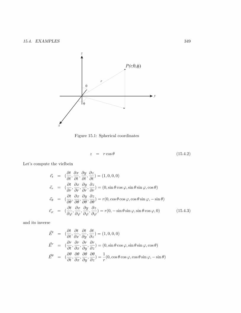
15.4. EXAMPLES 349
Figure 15.1: Spherical coordinates
z = r cos θ (15.4.2)
Let’s compute the vielbein
~et = (∂t
∂t,∂x
∂t,∂y
∂t,∂z
∂t) = (1, 0, 0, 0)
~er = (∂t
∂r,∂x
∂r,∂y
∂r,∂z
∂r) = (0, sin θ cosϕ, sin θ sinϕ, cos θ)
~eθ = (∂t
∂θ,∂x
∂θ,∂y
∂θ,∂z
∂θ) = r(0, cos θ cosϕ, cos θ sinϕ,− sin θ)
~eϕ = (∂t
∂ϕ,∂x
∂ϕ,∂y
∂ϕ,∂z
∂ϕ) = r(0,− sin θ sinϕ, sin θ cosϕ, 0) (15.4.3)
and its inverse
~Et = (∂t
∂t,∂t
∂x,∂t
∂y,∂t
∂z) = (1, 0, 0, 0)
~Er = (∂r
∂t,∂r
∂x,∂r
∂y,∂r
∂z) = (0, sin θ cosϕ, sin θ sinϕ, cos θ)
~Eθ = (∂θ
∂t,∂θ
∂x,∂θ
∂y,∂θ
∂z) =
1
r(0, cos θ cosϕ, cos θ sinϕ,− sin θ)
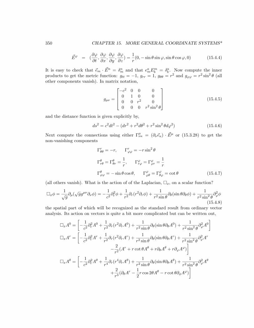
350 CHAPTER 15. MORE GENERAL COORDINATE SYSTEMS*
~Eϕ = (∂ϕ
∂t,∂ϕ
∂x,∂ϕ
∂y,∂ϕ
∂z) =
1
r(0,− sin θ sinϕ, sin θ cosϕ, 0) (15.4.4)
It is easy to check that ~em · ~En = δnm and that eamEmb = δab . Now compute the inner
products to get the metric function: gtt = −1, grr = 1, gθθ = r2 and gϕϕ = r2 sin2 θ (allother components vanish). In matrix notation,
gµν =
−c2 0 0 0
0 1 0 00 0 r2 00 0 0 r2 sin2 θ
(15.4.5)
and the distance function is given explicitly by,
ds2 = c2dt2 − (dr2 + r2dθ2 + r2 sin2 θdϕ2) (15.4.6)
Next compute the connections using either Γµνκ = (∂ν~eκ) · ~Eµ or (15.3.28) to get thenon-vanishing components
Γrθθ = −r, Γrϕϕ = −r sin2 θ
Γθrθ = Γθθr =1
r, Γϕrϕ = Γϕϕr =
1
r
Γθϕϕ = − sin θ cos θ, Γϕϕθ = Γϕθϕ = cot θ (15.4.7)
(all others vanish). What is the action of of the Laplacian, x, on a scalar function?
xφ =1√g∂µ(√ggµν∂νφ) = − 1
c2∂2t φ+
1
r2∂r(r
2∂rφ) +1
r2 sin θ∂θ(sin θ∂θφ) +
1
r2 sin2 θ∂2ϕφ
(15.4.8)the spatial part of which will be recognized as the standard result from ordinary vectoranalysis. Its action on vectors is quite a bit more complicated but can be written out,
xA0 =
[− 1
c2∂2tA
0 +1
r2∂r(r
2∂rA0) +
1
r2 sin θ∂θ(sin θ∂θA
0) +1
r2 sin2 θ∂2ϕA
0
]xA
r =
[− 1
c2∂2tA
r +1
r2∂r(r
2∂rAr) +
1
r2 sin θ∂θ(sin θ∂θA
r) +1
r2 sin2 θ∂2ϕA
r
− 2
r2(Ar + r cot θAθ + r∂θA
θ + r∂ϕAϕ)
]xA
θ =
[− 1
c2∂2tA
θ +1
r4∂r(r
4∂rAθ) +
1
r2 sin θ∂θ(sin θ∂θA
θ) +1
r2 sin2 θ∂2ϕA
θ
+2
r3(∂θA
r − 1
2r cos 2θAθ − r cot θ∂φA
ϕ)
]
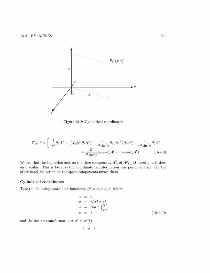
15.4. EXAMPLES 351
Figure 15.2: Cylindrical coordinates
xAϕ =
[− 1
c2∂2tA
ϕ +1
r4∂r(r
4∂rAϕ) +
1
r2 sin3 θ∂θ(sin
3 θ∂θAϕ) +
1
r2 sin2 θ∂2ϕA
ϕ
+2
r3 sin3 θ(sin θ∂ϕA
r + r cos θ∂ϕAθ)
](15.4.9)
We see that the Laplacian acts on the time component, A0, of Aµ, just exactly as it doeson a scalar. This is because the coordinate transformation was purely spatial. On theother hand, its action on the space components mixes them.
Cylindrical coordinates
Take the following coordinate functions: ξµ = (t, ρ, ϕ, z) where
t = tρ =
√x2 + y2
ϕ = tan−1(yx
)z = z (15.4.10)
and the inverse transformations: xa = xa(ξ)
t = t
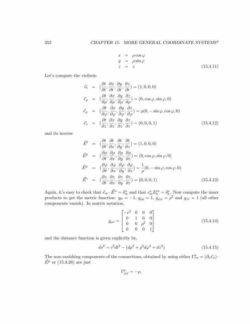
352 CHAPTER 15. MORE GENERAL COORDINATE SYSTEMS*
x = ρ cosϕy = ρ sinϕz = z (15.4.11)
Let’s compute the vielbein
~et = (∂t
∂t,∂x
∂t,∂y
∂t,∂z
∂t) = (1, 0, 0, 0)
~eρ = (∂t
∂ρ,∂x
∂ρ,∂y
∂ρ,∂z
∂ρ) = (0, cosϕ, sinϕ, 0)
~eϕ = (∂t
∂ϕ,∂x
∂ϕ,∂y
∂ϕ,∂z
∂ϕ) = ρ(0,− sinϕ, cosϕ, 0)
~ez = (∂t
∂z,∂x
∂z,∂y
∂z,∂z
∂z) = (0, 0, 0, 1) (15.4.12)
and its inverse
~Et = (∂t
∂t,∂t
∂x,∂t
∂y,∂t
∂z) = (1, 0, 0, 0)
~Eρ = (∂ρ
∂t,∂ρ
∂x,∂ρ
∂y,∂ρ
∂z) = (0, cosϕ, sinϕ, 0)
~Eϕ = (∂ϕ
∂t,∂ϕ
∂x,∂ϕ
∂y,∂ϕ
∂z) =
1
ρ(0,− sinϕ, cosϕ, 0)
~Ez = (∂z
∂t,∂z
∂x,∂z
∂y,∂z
∂z) = (0, 0, 0, 1) (15.4.13)
Again, it’s easy to check that ~em · ~En = δnm and that eamEmb = δab . Now compute the inner
products to get the metric function: gtt = −1, gρρ = 1, gϕϕ = ρ2 and gzz = 1 (all othercomponents vanish). In matrix notation,
gµν =
−c2 0 0 0
0 1 0 00 0 ρ2 00 0 0 1
(15.4.14)
and the distance function is given explicitly by,
ds2 = c2dt2 − (dρ2 + ρ2dϕ2 + dz2) (15.4.15)
The non-vanishing components of the connections, obtained by using either Γµνκ = (∂ν~eκ) ·~Eµ or (15.3.28) are just
Γρϕϕ = −ρ,
15.5. INTEGRATION: THE VOLUME ELEMENT 353
Γϕρϕ = Γϕϕρ =1
ρ(15.4.16)
(all others vanish), while the action of the Laplacian, x, on a scalar function is
xφ =1√g∂µ(√ggµν∂νφ) = − 1
c2∂2t φ+
1
ρ∂ρ(ρ∂ρφ) +
1
ρ2∂2ϕφ+ ∂2
zφ (15.4.17)
the spatial part of which being, as before, the standard result from ordinary vector analysis.Its action on vectors can be written out and we leave this as a straightforward exercise.4,5
15.5 Integration: The Volume Element
When passing from Cartesian coordinates to general coordinates one must also take careto account for the change in the integration measure, which follows the usual rule,∫
d4x→∫d4ξ
∥∥∥∥∂x∂ξ∥∥∥∥ (15.5.1)
where ||∂ξ/∂x|| represents the Jacobian of the transformation. Now notice that under thecoordinate transformation that took xa → ξµ, the metric also underwent a transformation
ηab → gµν = ηab∂xa
∂ξµ∂xa
∂ξµ= ηabe
aµebµ (15.5.2)
It follows, upon taking determinants, that
||g|| = ||η||∥∥∥∥∂x∂ξ
∥∥∥∥2
= −c2
∥∥∥∥∂x∂ξ∥∥∥∥2
(15.5.3)
where we have used ||η|| = −c2. Therefore,∥∥∥∥∂x∂ξ∥∥∥∥ =
1
c
√−||g|| (15.5.4)
We have previously used the notation g for the determinant of the metric, g. Continuingwith this notation we notice that (15.5.1) can be written as∫
d4x→ 1
c
∫d4ξ√−g (15.5.5)
4Problem: Write out xAµ for each component of Aµ in cylindrical coordinates.5Problem: Work out the details of the Rindler spacetime.

354 CHAPTER 15. MORE GENERAL COORDINATE SYSTEMS*
Again, we see that if the transformation is just a Lorentz transformation,∫d4x→
∫d4x′ (15.5.6)
because the metric gµν then continues to be just the Lorentz metric. Thus we are led todefine
1
c
∫d4ξ√−g (15.5.7)
as the correct volume integration measure in any system of coordinates. Simple examplesare spherical coordinates:
1
c
∫d4ξ√−g =
∫dt
∫dr r2
∫ π
0dθ sin θ
∫ 2π
0dϕ (15.5.8)
and cylindrical coordinates:
1
c
∫d4ξ√−g =
∫dt
∫dz
∫dρ ρ2
∫ 2π
0dϕ (15.5.9)
but (15.5.7) has general applicability.
Chapter 16
Ideal Fluids
16.1 Introduction
According to the atomic theory of Leucippus and his student Democritus, matter is dis-tinguished from space by the fact that it is not infinitely divisible. If we accept this atomictheory, a truly “continuous” medium, defined as matter that is infinitely divisible, cannotreally exist in nature. Yet, there are situations in which a system of particles may betreated as though it were a “continuous medium”. To understand what these situationsare, let R represent a typical length scale over which observations are carried out on asystem of particles, let a be the characteristic size of the particles and let N be the numberof particles within a volume determined by R. The length scale R could be, for example,the size of a body immersed in the system of particles or the size of an imaginary volumeelement within the system. Suppose we are interested in describing the motion of theimmersed body, or, more generally, of an imaginary volume element, without regard tothe individual motions of the molecules. We will treat a medium as “continuous” if themean free path, 〈l〉, of the particles is much smaller than the scale R. For example, air canbe considered a continuous medium for the propagation of sound waves provided that thewavelength of the wave is large compared with the mean free path of the air molecules.At shorter wavelengths the air stops behaving as a continuous medium. More precisely,in terms of the Knudsen number
K =〈l〉R, (16.1.1)
the collection of particles is deemed continuous if K 1 at all times. The number densityof particles in a spherical volume of radius R being roughly N/R3, the mean free path ofthe particles is given by the Clausius relation,
〈l〉 ≈ R3
√2πa2N
, (16.1.2)
355
356 CHAPTER 16. IDEAL FLUIDS
where a is a typical atomic or molecular size, from which it follows that for the system ofparticles to be treated as constituting a continuous medium, we should require that
√N R
a(16.1.3)
Typically the distance scales over which a classical experiment is carried out is very muchlarger than the molecular size, so the condition implies that both N and R/a are muchgreater than unity.
If an equation of state is available, the condition (16.1.1) may be framed in terms ofthe state variables of the system. For example for a classical, ideal gas the equation ofstate p = nkT , where n is the number density of molecules and p is the pressure of thegas, implies that
K =kT√
2πa2pR 1 (16.1.4)
should hold at all times. An equivalent way to define the continuum approximation is tosay that a typical molecule undergoes a very large number of collisions in traversing theexperimental distance scale R.
When (16.1.1) holds it it no longer necessary to concern oneself with the individualmotions of the molecules. One concentrates instead on the motion of the medium as awhole, thereby gaining relative simplicity but losing the ability to describe the mediummicroscopically. Thus we consider volumes of the fluid that are “microscopically large butmacroscopically small” i.e., small enough to be treated as infinitesimal volume elementsbut large enough to contain a very large number of particles. In the process the molecularsize is essentially shrunk to zero and the molecules are treated as if they are point-like.This is the continuum approximation.
Continuous media can be divided into solids, liquids and gases, the latter two beinggenerally classified as “fluids”. The essential difference between them is the strengthof the interaction between the particles (molecules) that consitute the medium. Theseinteractions are very strong in solids and weak in differing degrees for fluids, being weakestfor gases. When we say “strong” and “weak” we are of course referring to the ratio betweenthe binding energy of the constituents, 〈Eb〉, and the typical thermal excitation energykT . If 〈Eb〉/kT 1 the medium is solid, but if 〈Eb〉/kT . 1 the medium is a liquidor gas because thermal excitations or relatively weak mechanical forces are able to breakthe inter-particle bonds and cause the medium to flow. For this reason, solids turn intoliquids and gases at high enough temperatures, according to our common experience. Inthis chapter we concentrate on fluids.
A fluid is described by five fields, viz.,
• The three components of a velocity vector field, ~v(~r, t), which gives the averagevelocity of a molecule at any point, ~r, within the fluid at any time, t,
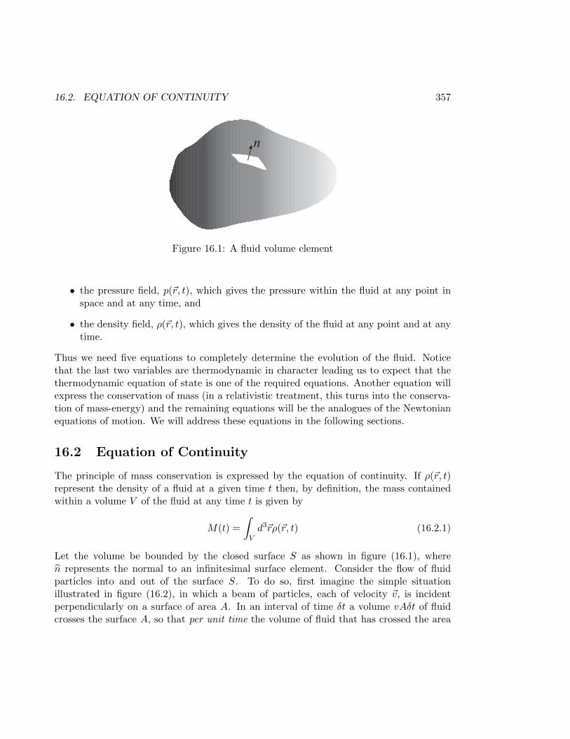
16.2. EQUATION OF CONTINUITY 357
n
Figure 16.1: A fluid volume element
• the pressure field, p(~r, t), which gives the pressure within the fluid at any point inspace and at any time, and
• the density field, ρ(~r, t), which gives the density of the fluid at any point and at anytime.
Thus we need five equations to completely determine the evolution of the fluid. Noticethat the last two variables are thermodynamic in character leading us to expect that thethermodynamic equation of state is one of the required equations. Another equation willexpress the conservation of mass (in a relativistic treatment, this turns into the conserva-tion of mass-energy) and the remaining equations will be the analogues of the Newtonianequations of motion. We will address these equations in the following sections.
16.2 Equation of Continuity
The principle of mass conservation is expressed by the equation of continuity. If ρ(~r, t)represent the density of a fluid at a given time t then, by definition, the mass containedwithin a volume V of the fluid at any time t is given by
M(t) =
∫Vd3~rρ(~r, t) (16.2.1)
Let the volume be bounded by the closed surface S as shown in figure (16.1), wheren represents the normal to an infinitesimal surface element. Consider the flow of fluidparticles into and out of the surface S. To do so, first imagine the simple situationillustrated in figure (16.2), in which a beam of particles, each of velocity ~v, is incidentperpendicularly on a surface of area A. In an interval of time δt a volume vAδt of fluidcrosses the surface A, so that per unit time the volume of fluid that has crossed the area
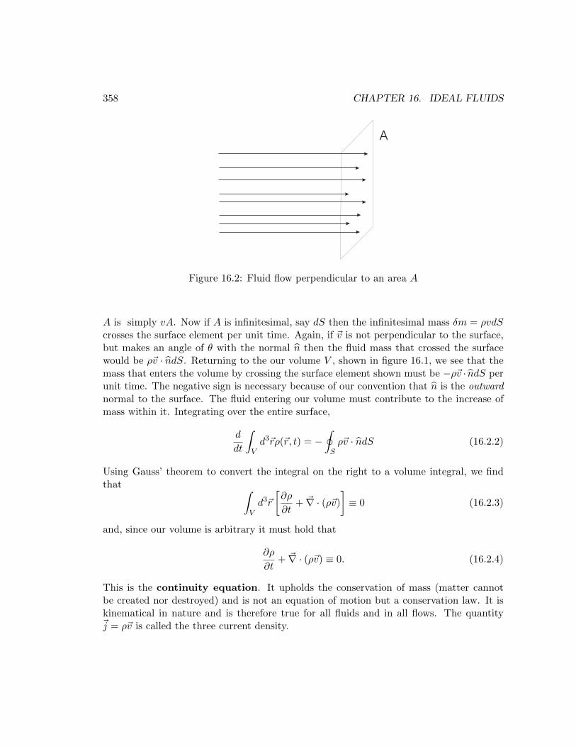
358 CHAPTER 16. IDEAL FLUIDS
A
Figure 16.2: Fluid flow perpendicular to an area A
A is simply vA. Now if A is infinitesimal, say dS then the infinitesimal mass δm = ρvdScrosses the surface element per unit time. Again, if ~v is not perpendicular to the surface,but makes an angle of θ with the normal n then the fluid mass that crossed the surfacewould be ρ~v · ndS. Returning to the our volume V , shown in figure 16.1, we see that themass that enters the volume by crossing the surface element shown must be −ρ~v · ndS perunit time. The negative sign is necessary because of our convention that n is the outwardnormal to the surface. The fluid entering our volume must contribute to the increase ofmass within it. Integrating over the entire surface,
d
dt
∫Vd3~rρ(~r, t) = −
∮Sρ~v · ndS (16.2.2)
Using Gauss’ theorem to convert the integral on the right to a volume integral, we findthat ∫
Vd3~r
[∂ρ
∂t+ ~∇ · (ρ~v)
]≡ 0 (16.2.3)
and, since our volume is arbitrary it must hold that
∂ρ
∂t+ ~∇ · (ρ~v) ≡ 0. (16.2.4)
This is the continuity equation. It upholds the conservation of mass (matter cannotbe created nor destroyed) and is not an equation of motion but a conservation law. It iskinematical in nature and is therefore true for all fluids and in all flows. The quantity~j = ρ~v is called the three current density.
16.3. IDEAL FLUIDS 359
16.3 Ideal Fluids
An ideal fluid will be one in which there is no dissipation of energy within the fluid. Micro-scopically, internal energy dissipation occurs via inelastic collisions between the moleculesof the fluid, so an ideal fluid is one in which the intermolecular collisions are elastic. Wewill also assume for the present that there is no energy transfer between the fluid and itsenvironment through its boundaries. The absence of heat exchange between the variousparts of the fluid and between the fluid and its boundaries implies that the flow is isen-tropic, i.e., that the flow is such that the entropy per particle is constant throughout itsevolution. The entropy, like the pressure, will depend on the spatial position within thefluid as well as on time. Let s be the entropy per unit mass. An isentropic flow requiresthat
ds
dt=∂s
∂t+ (~v · ~∇)s = 0 (16.3.1)
and if we combine this with the continuity equation, we find that
∂
∂t(ρs) =
∂ρ
∂ts+ ρ
∂s
∂t
= −~∇ · (ρ~v)s− ρ(~v · ~∇)s
= −~∇ · (ρs~v) (16.3.2)
where we have used (16.2.4). Thus,
∂(ρs)
∂t+ ~∇ · (ρs~v) ≡ 0, (16.3.3)
which is the continuity equation expressing entropy conservation in the same terms as(16.2.4) expresses mass conservation. The quantity ρs is the entropy density and ~σ = ρs~vis the entropy current three density.
16.4 Euler’s equation for an Ideal Fluid
Euler’s equations are the precise analogues for a fluid of Newton’s equations for a particle.They therefore define the dynamics of the ideal fluid and will need to be modified whenwe want to take into account energy dissipation and heat transfer within the fluid andbetween the fluid and its environment.
Consider a volume V of fluid as shown in (16.1) and recall that this volume lies withinthe fluid. Due to the surrounding medium, which exerts a pressure on the surface boundingthe volume, there will be a net force on the volume which is given by
~F = −∮Spn · dS (16.4.1)
360 CHAPTER 16. IDEAL FLUIDS
Again, it can be expressed in terms of a volume integral by Gauss’ theorem
~F = −∫Vd3~r ~∇p. (16.4.2)
The total force on the volume V is the force due to the rest of the fluid as well as theforce exerted by the environment on the volume, which we will simply refer to as ~F ext. Itis preferable, however, to work in terms of force densities, so let us define ~f ext as
~F ext =
∫Vd3~r ~f ext (16.4.3)
To apply Newton’s second law, we must ask what constitutes the left hand side. For therate of change of momentum associated with the volume we have
d
dt
∫Vd3~r(ρ~v). (16.4.4)
but we must add to this a term that accounts for the rate of change of momentum asso-ciated with the surface deformations. This is1∮
SdS ρ~v(n · ~v) (16.4.5)
Newton’s second law of motion then takes the form
d
dt
∫Vd3~r(ρ~v) +
∮SdS ρ~v(n · ~v) = −
∫Vd3~r ~∇p+
∫Vd3~r ~f ext (16.4.6)
where ρ~v is the momentum density of the fluid in our volume element. The first term onthe left hand side is ∫
Vd3~r
[ρ∂~v
∂t+ ~v
∂ρ
∂t
]=
∫Vd3~r
[ρ∂~v
∂t− ~v~∇ · (ρ~v)
](16.4.7)
where we used the equation of continuity. Let us consider the second term in components(Einstein’s summation convention is assumed throughout). We have
−vi∂j(ρvj) = −∂j(ρvivj) + ρvj∂jvi
⇒ −~v~∇ · (ρ~v) = −~∇ · (~v ⊗ ~v) + ρ(~v · ~∇)~v (16.4.8)
Upon integrating over the volume V and applying Gauss’ theorem, the first term on theright turns into
−∮SdS ρ~v(n · ~v) (16.4.9)
1This comes from the theory of elasticity and here we shall take it as given.

16.4. EULER’S EQUATION FOR AN IDEAL FLUID 361
and cancels the second term on the left of (16.4.6) leaving∫Vd3~r
[ρ∂~v
∂t+ ρ(~v · ~∇)~v
]= −
∫Vd3~r ~∇p+
∫Vd3~r ~f ext. (16.4.10)
Again, because the volume we are considering is arbitrary, it follows that
ρ∂~v
∂t+ ρ(~v · ~∇)~v = −~∇p+ ~f ext (16.4.11)
These are Euler’s equations for an ideal fluid. Notice that the left hand side is nothingbut the total derivative of ~v(~r, t), in terms of which the equations could be written as
ρd~v
dt= −~∇p+ ~f ext. (16.4.12)
The left hand side is called the “total” acceleration of the fluid. It is made up of two parts,one of which, ∂~v/∂t, measures the rate of change of velocity at a fixed point and is calledthe local acceleration. The other is the term (~v · ~∇)~v and represents a contribution tothe rate of change of velocity from a change in location within the fluid. It is called theconvective acceleration.
The external force in equation (16.4.12) is expected from a naıve application of New-ton’s second law to a unit volume of fluid, without explicitly taking into account the surfaceterms. As an example of an external force, consider a fluid in a constant gravitationalfield ~g(~r, t). Euler’s equations would read
ρ∂~v
∂t+ ρ(~v · ~∇)~v = −~∇p+ ρ~g. (16.4.13)
The five equations governing the motion of an ideal fluid are therefore
• an equation of state, f(p, T, ρ) = 0,
• the continuity equation in (16.2.4) and
• Euler’s equations in (16.4.11)
For an isentropic flow one can trade the pressure for the enthalpy per unit mass. Thissimplifies Euler’s equations. Because the enthalpy,
H = U + pV, (16.4.14)
where U , the internal energy of the system, is an extensive quantity. Define the enthalpyper unit mass by h = u + p/ρ, where u is the internal energy per unit mass and v = 1/ρis the volume occupied by a unit mass. Then
dh = du+dp
ρ− p
ρ2dρ (16.4.15)

362 CHAPTER 16. IDEAL FLUIDS
and because the internal energy per unit mass obeys the first law of thermodynamics
du = Tds− pd(
1
ρ
)= Tds+
p
ρ2dρ (16.4.16)
where s is the entropy per unit mass of the fluid, it follows that
dh = Tds+p
ρ2dρ+
dp
ρ− p
ρ2dρ = Tds+
dp
ρ(16.4.17)
i.e., the enthalpy is a function of (s, p). Since ds = 0 for an isentropic flow, we havedh = dp/ρ⇒ ~∇p = ρ~∇h and Euler’s equations can be written in terms of h
d~v
dt= −~∇h+
~f ext
ρ. (16.4.18)
This is the second form of Euler’s equations. Taking the curl of this equation we get
∂
∂t(~∇× ~v) + ~∇× (~v · ~∇)~v = −~∇×
(~f ext
ρ
)(16.4.19)
where we have used the fact that the curl of a gradient vanishes identically. Now2
~∇× [~v × (~∇× ~v)] = ~∇×(
1
2~∇~v2 − (~v · ~∇)~v
)= −~∇× (~v · ~∇)~v (16.4.20)
and therefore∂
∂t(~∇× ~v) = ~∇× [~v × (~∇× ~v)] + ~∇×
(~f ext
ρ
), (16.4.21)
or∂~ω
∂t− ~∇× (~v × ~ω) = ~∇×
(~f ext
ρ
), (16.4.22)
where ω = ~∇× ~v is called the vorticity of the flow. This is sometimes referred to as thethird form of Euler’s equations.
16.5 Waves in Fluids
The set of five equations, viz., Euler’s equations, the equation of continuity and the equa-tion of state imply the existence of (sound) waves in fluids. Consider a simplified situation
2 Problem: Prove this.
16.6. SPECIAL FLOWS 363
in which the fluid is static, i.e., ~v = 0 and of uniform density (ρ = ρ0) and pressure(p = p0). Now examine small perturbations about this equilibrium,
~v = δ~v(~r, t), ρ = ρ0 + δρ(~r, t), p = p0 + δp(~r, t), (16.5.1)
then by the continuity equation and to first order
∂δρ
∂t+ ρ0
~∇ · δ~v = 0. (16.5.2)
Likewise, by Euler’s equation,∂δ~v
∂t= − 1
ρ0
~∇δp (16.5.3)
To complete the set we need to exploit the equation of state. Imagine that the propagationof the perturbations occurs under certain conditions (eg. isothermal or adiabatic), andtake it to be of the form p = p(ρ), so that p0 = p(ρ0) and δp = p′(ρ0)δρ. Taking a secondtime derivative of the continuity equation and using Euler’s equations,
∂2δρ
∂t2− c2~∇2δρ = 0, c2 = p′(ρ0), (16.5.4)
which is the equation for sound waves traveling at
c =
öp
∂ρ
∣∣∣∣∣ρ=ρ0
. (16.5.5)
For example, consider an ideal gas in which waves propagate under isothermal conditions.Then p′(ρ0) = kT/m, where m is the molecular mass of the gas, and we recover (8.2.22).If we consider adiabatic propagation instead then the equation of state, p = const. × ργ ,implies that p′(ρ0) = γkT/m, where γ is the ratio of heat capacities, γ = Cp/CV , and thisreproduces (8.2.21).
16.6 Special Flows
We now consider some special flows for which Euler’s equations become greatly simplified.
16.6.1 Hydrostatics
For static fluids the velocity field is vanishing everywhere at all times and Euler’s equationsreduce to
~∇p = ~f ext (16.6.1)
This is the “equation of hydrostatics”. It must be supplemented by the condition (fromthe continuity equation) that ρ does not depend explicitly on time, i.e., ∂ρ/∂t = 0.
364 CHAPTER 16. IDEAL FLUIDS
16.6.2 Steady Flows
A steady flow is one for which the velocity does not depend explicitly on time, i.e., onefor which ∂~v/∂t = 0. In this case Euler’s equations become
ρ(~v · ~∇)~v = −~∇p+ ~f ext (16.6.2)
and using
~v × (~∇× ~v) =1
2~∇~v2 − (~v · ~∇)~v (16.6.3)
we find1
2~∇~v2 − ~v × (~∇× ~v) + ~∇h =
~f ext
ρ(16.6.4)
Taking the inner product with the unit vector that points in the direction of ~v we get
v · ~∇[
1
2~v2 + h
]=v · ~f ext
ρ(16.6.5)
where we made use of the fact that the term ~v × (~∇× ~v) is perpendicular to both ~v and~∇×~v. Now if the force per unit mass is derivable from a potential per unit mass accordingto the usual relation
~f ext
ρ= −~∇Φ (16.6.6)
then (16.6.5) turns into
v · ~∇[
1
2~v2 + h+ Φ
]≡ 0 (16.6.7)
This takes a bit of interpreting. Notice that v · ~∇ represents the directional derivative alonga curve whose tangent at any point is the velocity. Such curves are called streamlinesand (16.6.7) says that the directional derivative along a streamline vanishes, or alongstreamlines
1
2~v2 + h+ Φ = const. (16.6.8)
This is Bernoulli’s equation and expresses the conservation of energy. It is very im-portant to emphasize that this holds only along streamlines because the constant on theright hand side may vary from streamline to streamline. To appreciate the significance ofa streamline, notice that because the velocity has no explicit dependence on t therefore atany point P (~rP ) it is always constant. The typical (average) molecule at P would havevelocity ~vP , so its displacement in a time interval δt would be
δ~rP = ~vP δt (16.6.9)
16.6. SPECIAL FLOWS 365
However, at point ~rP + δ~rP its velocity is once again fixed, which would then determineits further development. Thus molecules that find themselves at P would, on the average,follow the same trajectory. This trajectory is unique to molecules that pass through P andis called a streamline. Two streamlines may not cross one another. If they did then, at theintersection point, the velocity field would not be single valued. Neither can a streamlinebifurcate at any point. If it did then, at the bifurcation point, the acceleration would notbe single valued. Mathematically, streamlines are the integral curves of the velocity vectorfield,
d~r
dt= ~v ⇒ dx
vx=dy
vy=dz
vz. (16.6.10)
When ~v does depend explicitly on t the concept of a streamline is no longer useful as themolecules passing through P would have, on the average, different velocities depending onthe time at which they passed through P .
Bernoulli’s equation is further simplified when the fluid is incompressible, i.e., whenρ(~r, t) is constant. In this case, the continuity equation requires that
~∇ · ~v = 0 (16.6.11)
Furthermore, dh = dp/ρ = d(p/ρ) allows us to write Bernoulli’s equation in the form
v · ~∇[
1
2ρ~v2 + p+ ρΦ
]≡ 0 (16.6.12)
or
p+1
2ρ~v2 + ρΦ = const. (16.6.13)
along streamlines. For example, if Φ represents a constant gravitational potential then
p+1
2ρ~v2 + ρgz = const. (16.6.14)
where we have assumed that the gravitational field is oriented in the negative z direction.In general incompressibility implies that the velocity field is derivable from a vector
potential, ~v = ~∇ × ~V , because the divergence of a curl is identically zero. However, intwo dimensional flows incompressibility implies that ~v is derivable from a scalar potential,ψ(x, y), according to
vx = ∂yψ, vy = −∂xψ. (16.6.15)
The equation ψ(x, y) = const. gives the streamlines.3
3This follows because, according to (16.6.10),
vxdy − vydx = ∂xψdx+ ∂yψdy = 0
⇒ dψ = 0⇒ ψ(x, y) = const.
366 CHAPTER 16. IDEAL FLUIDS
16.6.3 Irrotational or Potential Flows
The vorticity ~ω of a flow is defined by ~ω = ~∇ × ~v. If the vorticity is everywhere zerothen the flow is said to be “irrotational”. Irrotational flows are also called potentialflows because the condition ~∇×~v = 0 implies that the velocity vector is derivable from apotential, i.e., ~v = ~∇ψ for some scalar function ψ(~r, t). Let us see what Euler’s equationsturn into when we demand that the flow be irrotational. From the third form of Euler’sequations we see immediately that irrotational flows can exist only if the external force perunit mass is also irrotational. Let Φ be the potential energy per unit mass, then inserting~v = ~∇ψ in the first form of the equations we have
~∇∂ψ∂t
+ (~∇ψ · ~∇)~∇ψ = −~∇(h+ Φ) (16.6.16)
Now in components
[(~∇ψ · ~∇)~∇ψ]i = ∂jψ∂j(∂iψ) = ∂jψ∂i(∂jψ), (16.6.17)
where we have applied the integrability condition, so that
(~∇ψ · ~∇)~∇ψ =1
2~∇(~∇ψ)2 (16.6.18)
and therefore
~∇[∂ψ
∂t+
1
2(~∇ψ)2 + h+ Φ
]≡ 0 (16.6.19)
or∂ψ
∂t+
1
2(~∇ψ)2 + h+ Φ = f(t) (16.6.20)
where f(t) is an arbitrary function of t. This function can be set to be constant, however,because from the definition of ~v in terms of ψ it is clear that
ψ → ψ +
∫f(t)dt+ const. (16.6.21)
does not change ~v but does eliminate f(t) in (16.6.20). After all, it is not ψ that ismeasured but ~v. As for any potential, ψ is arbitrary up to some redefinition. This isBernoulli’s equation for irrotational flows, with one important distinction. Whereas theconstant on the right hand side of (16.6.8) is different in principle from streamline tostreamline it is the same for all streamlines in (16.6.20).
16.7. ELEMENTARY APPLICATIONS 367
16.6.4 Incompressible Flows
An incompressible flow is one for which dρ/dt = 0, i.e., by the equation of continuity,~∇ ·~v = 0. The third form of Euler’s equation is seen to be an equation for the vorticity ofa flow,
∂~ω
∂t− ~∇× (~v × ~ω) = ~∇×
(~f ext
ρ
)(16.6.22)
Expanding the left hand side of this equation,
∂~ω
∂t− (~ω · ~∇)~v + (~v · ~∇)~ω + ~ω(~∇ · ~v)− ~v(~∇ · ~ω) = ~∇×
(~f ext
ρ
)(16.6.23)
and since ~∇ · ~ω ≡ 0, we find a simplified equation when the fluid is also incompressible(~∇ · ~v = 0),
d~ω
dt= (~ω · ~∇)~v + ~∇×
(~f ext
ρ
)(16.6.24)
or justd~ω
dt= (~ω · ~∇)~v (16.6.25)
in the absence of external force fields. If an incompressible fluid undergoes irrotationalflow then ~v = ~∇ψ and Euler’s equations are automatic. Moreover the incompressibilitycondition, ~∇ · ~v = 0, turns into the equation ~∇2ψ = 0.
16.7 Elementary Applications
16.7.1 Hydrostatics
We will now look at some simple applications of the above types of flow, beginning withthe simplest of all: hydrostatics. In this case, because ~v(~r, t) is constrained to be vanishingwe have just
~∇p = ~f ext (16.7.1)
which expresses the fact that the force per unit volume is balanced by the pressure withinthe fluid. If the external force density is due to a homogeneous external gravitational field~g in, say, the negative z direction then
∂p
∂x=∂p
∂y= 0,
∂p
∂z= −ρg (16.7.2)
and the first two equations imply only that p = p(z). The last equation will have differentsolutions depending on whether or not the fluid is compressible.
368 CHAPTER 16. IDEAL FLUIDS
If the fluid is incompressible then the solution is trivially
p(z) = p0 − ρg(z − z0) = p0 + ρg(z0 − z) (16.7.3)
where p0 is the pressure at z = z0. The quantity z− z0 will be referred to as the “height”and z0−z as the “depth”. The formula gives the variation of pressure with height (depth)assuming that the fluid is effectively incompressible. This approximation is generallyreasonable in liquids up to a certain depth (depending on the liquid) but is not very usefulin treating gases.
If the fluid is compressible, the density is a non-trivial function of the pressure andtemperature. Consider a column of an ideal gas at a fixed absolute temperature T . Usingthe equation of state
p = nkT =ρkT
m⇒ ρ =
mp
kT(16.7.4)
where m is the molecular mass, we find
dp
p= −mg
kTdz ⇒ p = p0e
−mgkT
(z−z0) (16.7.5)
where p0 is the pressure at z0. Now if the absolute temperature is also a function of z, thesolution will be more complex. For example, if T (z) = T0− γ(z− z0) where γ is a positiveconstant called the “lapse rate” the equation to be solved is
dp
p= − mg
k[T0 − γ(z − z0)]dz ⇒ p = p0
[1− γ(z − z0)
T0
]mgkγ
(16.7.6)
In this solution T0 and p0 represent the temperature and pressure respectively at z = z0.It may also turn out that the fluid is not in a constant, homogeneous external gravi-
tational field as we have examined. For example a star can be thought of as a very largemass of gass that is held together by its own gravitational attraction. In the simplestcase of a star that is not rotating we can think of it as made up of spherical shells, eachshell being subject to the gravitational potential due to all the shells within it. The forcedensity is then ~f ext = −ρ~∇Φ where Φ represents this potential energy and from Gauss’law
~∇2Φ = −4πGρ (16.7.7)
Inserting Φ, dividing throught by the density and taking a divergence of the hydrostaticequation (16.6.1) gives
~∇ ·
(~∇pρ
)= −~∇2Φ = 4πGρ (16.7.8)
This equation must then be solved subject to some equation of state relating (p, ρ, T ) andsome assumptions regarding the variation of T with the radius r.
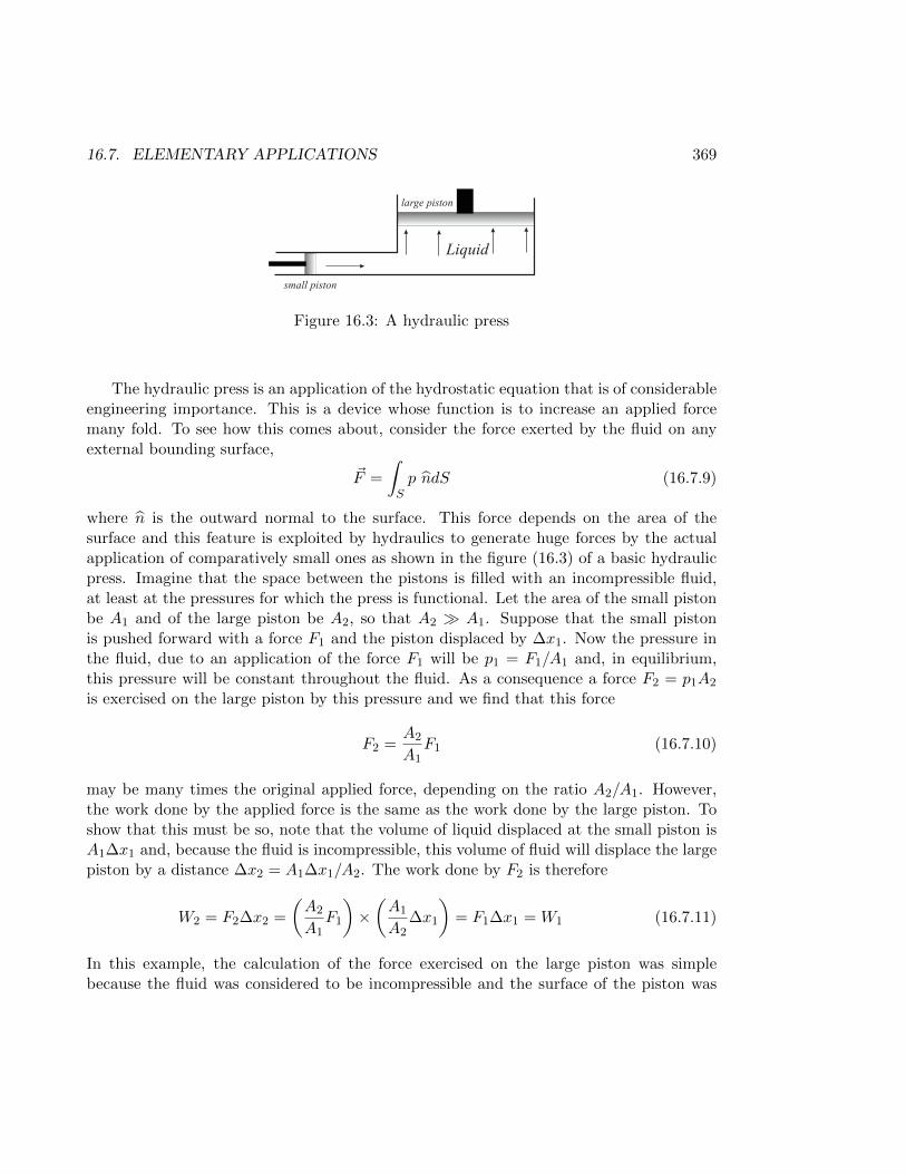
16.7. ELEMENTARY APPLICATIONS 369
Liquid
small piston
large piston
Figure 16.3: A hydraulic press
The hydraulic press is an application of the hydrostatic equation that is of considerableengineering importance. This is a device whose function is to increase an applied forcemany fold. To see how this comes about, consider the force exerted by the fluid on anyexternal bounding surface,
~F =
∫Sp ndS (16.7.9)
where n is the outward normal to the surface. This force depends on the area of thesurface and this feature is exploited by hydraulics to generate huge forces by the actualapplication of comparatively small ones as shown in the figure (16.3) of a basic hydraulicpress. Imagine that the space between the pistons is filled with an incompressible fluid,at least at the pressures for which the press is functional. Let the area of the small pistonbe A1 and of the large piston be A2, so that A2 A1. Suppose that the small pistonis pushed forward with a force F1 and the piston displaced by ∆x1. Now the pressure inthe fluid, due to an application of the force F1 will be p1 = F1/A1 and, in equilibrium,this pressure will be constant throughout the fluid. As a consequence a force F2 = p1A2
is exercised on the large piston by this pressure and we find that this force
F2 =A2
A1F1 (16.7.10)
may be many times the original applied force, depending on the ratio A2/A1. However,the work done by the applied force is the same as the work done by the large piston. Toshow that this must be so, note that the volume of liquid displaced at the small piston isA1∆x1 and, because the fluid is incompressible, this volume of fluid will displace the largepiston by a distance ∆x2 = A1∆x1/A2. The work done by F2 is therefore
W2 = F2∆x2 =
(A2
A1F1
)×(A1
A2∆x1
)= F1∆x1 = W1 (16.7.11)
In this example, the calculation of the force exercised on the large piston was simplebecause the fluid was considered to be incompressible and the surface of the piston was
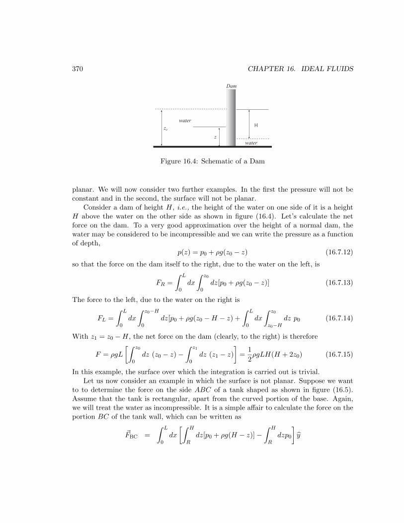
370 CHAPTER 16. IDEAL FLUIDS
H
z
z0
water
water
Dam
Figure 16.4: Schematic of a Dam
planar. We will now consider two further examples. In the first the pressure will not beconstant and in the second, the surface will not be planar.
Consider a dam of height H, i.e., the height of the water on one side of it is a heightH above the water on the other side as shown in figure (16.4). Let’s calculate the netforce on the dam. To a very good approximation over the height of a normal dam, thewater may be considered to be incompressible and we can write the pressure as a functionof depth,
p(z) = p0 + ρg(z0 − z) (16.7.12)
so that the force on the dam itself to the right, due to the water on the left, is
FR =
∫ L
0dx
∫ z0
0dz[p0 + ρg(z0 − z)] (16.7.13)
The force to the left, due to the water on the right is
FL =
∫ L
0dx
∫ z0−H
0dz[p0 + ρg(z0 −H − z) +
∫ L
0dx
∫ z0
z0−Hdz p0 (16.7.14)
With z1 = z0 −H, the net force on the dam (clearly, to the right) is therefore
F = ρgL
[∫ z0
0dz (z0 − z)−
∫ z1
0dz (z1 − z)
]=
1
2ρgLH(H + 2z0) (16.7.15)
In this example, the surface over which the integration is carried out is trivial.Let us now consider an example in which the surface is not planar. Suppose we want
to to determine the force on the side ABC of a tank shaped as shown in figure (16.5).Assume that the tank is rectangular, apart from the curved portion of the base. Again,we will treat the water as incompressible. It is a simple affair to calculate the force on theportion BC of the tank wall, which can be written as
~FBC =
∫ L
0dx
[∫ H
Rdz[p0 + ρg(H − z)]−
∫ H
Rdzp0
]y
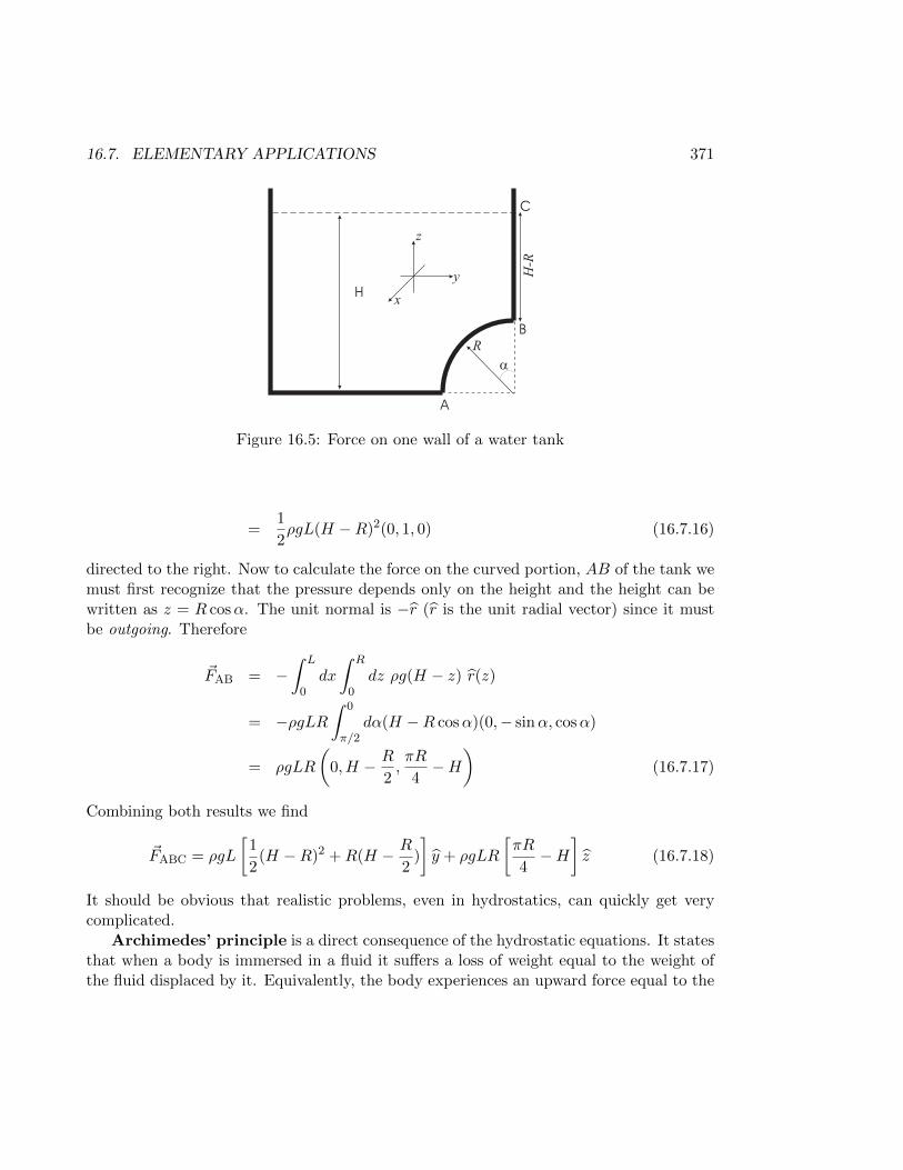
16.7. ELEMENTARY APPLICATIONS 371
H
A
B
R
a
H-R
C
y
z
x
Figure 16.5: Force on one wall of a water tank
=1
2ρgL(H −R)2(0, 1, 0) (16.7.16)
directed to the right. Now to calculate the force on the curved portion, AB of the tank wemust first recognize that the pressure depends only on the height and the height can bewritten as z = R cosα. The unit normal is −r (r is the unit radial vector) since it mustbe outgoing. Therefore
~FAB = −∫ L
0dx
∫ R
0dz ρg(H − z) r(z)
= −ρgLR∫ 0
π/2dα(H −R cosα)(0,− sinα, cosα)
= ρgLR
(0, H − R
2,πR
4−H
)(16.7.17)
Combining both results we find
~FABC = ρgL
[1
2(H −R)2 +R(H − R
2)
]y + ρgLR
[πR
4−H
]z (16.7.18)
It should be obvious that realistic problems, even in hydrostatics, can quickly get verycomplicated.
Archimedes’ principle is a direct consequence of the hydrostatic equations. It statesthat when a body is immersed in a fluid it suffers a loss of weight equal to the weight ofthe fluid displaced by it. Equivalently, the body experiences an upward force equal to the
372 CHAPTER 16. IDEAL FLUIDS
weight of the fluid displaced. The upward force is called the buoyancy and is the reasonboats and ships float. To understand how this comes about, suppose that the density ofthe fluid is ρf and that the density of the body itself is ρ. Let S be the surface boundingthe body, so that the net force on the body is
~F = −∮Spd~S +
∫Vd3~r ~f ext (16.7.19)
where ~f ext is the external force density which we take to be due to an external, homo-geneous gravitational field, i.e., ~f ext = ρg(0, 0,−1) directed in the negative z direction.Now, if the fluid is incompressible then p = p0 + ρfg(H − z) where H − z represents thedepth from the surface of the fluid and p0 represents the atmospheric pressure. Thus
~∇p = (0, 0,−ρfg) (16.7.20)
and therefore, applying Gauss’ theorem,
~F = −∫Vd3~r[0, 0, (ρ− ρf )g] = (ρf − ρ)gV z (16.7.21)
Now ρfV is the mass of liquid having the same volume as the immersed body itself and istherefore the mass of the fluid displaced by the body. The first term therefore representsthe buoyancy. Naturally a body will float so long as the buoyancy can overcome its weighti.e., ρf ≥ ρ. If ρf > ρ only a portion of the body, of volume V ′ < V , is immersed. Thefraction of the body’s volume that is immersed is given by the condition ρfV
′ = ρV or
V ′ =ρ
ρfV (16.7.22)
16.7.2 Steady Flows
Let us now examine some examples of steady flows. In this case, Euler’s equation reducesto
ρ(~v · ~∇)~v = −~∇p+ ~f ext (16.7.23)
a first integral of which is the Bernoulli equation
1
2~v2 + h+ Φ = const. (16.7.24)
along any streamline. Let us assume that ρ also does not depend explicitly on time. Inother words, that the system is in equilibrium. By continuity, this is only possible if
~∇ · (ρ~v) = 0 (16.7.25)
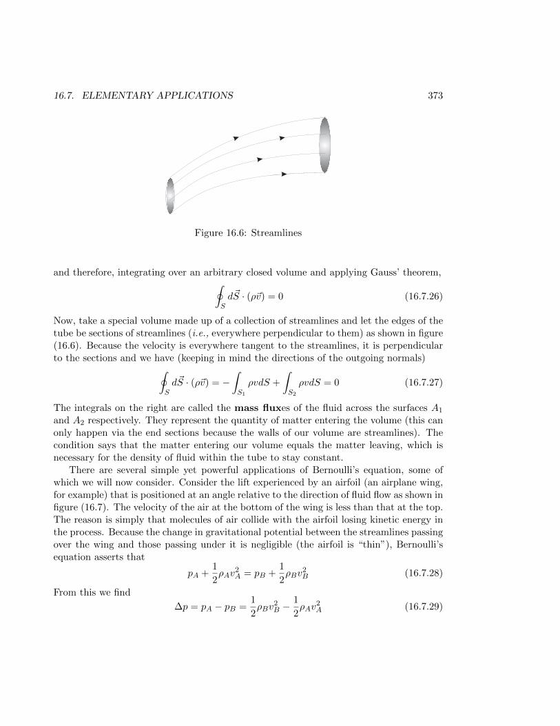
16.7. ELEMENTARY APPLICATIONS 373
Figure 16.6: Streamlines
and therefore, integrating over an arbitrary closed volume and applying Gauss’ theorem,∮Sd~S · (ρ~v) = 0 (16.7.26)
Now, take a special volume made up of a collection of streamlines and let the edges of thetube be sections of streamlines (i.e., everywhere perpendicular to them) as shown in figure(16.6). Because the velocity is everywhere tangent to the streamlines, it is perpendicularto the sections and we have (keeping in mind the directions of the outgoing normals)∮
Sd~S · (ρ~v) = −
∫S1
ρvdS +
∫S2
ρvdS = 0 (16.7.27)
The integrals on the right are called the mass fluxes of the fluid across the surfaces A1
and A2 respectively. They represent the quantity of matter entering the volume (this canonly happen via the end sections because the walls of our volume are streamlines). Thecondition says that the matter entering our volume equals the matter leaving, which isnecessary for the density of fluid within the tube to stay constant.
There are several simple yet powerful applications of Bernoulli’s equation, some ofwhich we will now consider. Consider the lift experienced by an airfoil (an airplane wing,for example) that is positioned at an angle relative to the direction of fluid flow as shown infigure (16.7). The velocity of the air at the bottom of the wing is less than that at the top.The reason is simply that molecules of air collide with the airfoil losing kinetic energy inthe process. Because the change in gravitational potential between the streamlines passingover the wing and those passing under it is negligible (the airfoil is “thin”), Bernoulli’sequation asserts that
pA +1
2ρAv
2A = pB +
1
2ρBv
2B (16.7.28)
From this we find
∆p = pA − pB =1
2ρBv
2B −
1
2ρAv
2A (16.7.29)
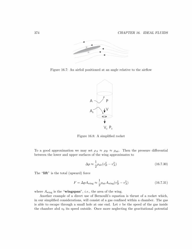
374 CHAPTER 16. IDEAL FLUIDS
A
B
Figure 16.7: An airfoil positioned at an angle relative to the airflow
V0
VA
0
A P
P0
Figure 16.8: A simplified rocket
To a good approximation we may set ρA ≈ ρB ≈ ρair. Then the pressure differentialbetween the lower and upper surfaces of the wing approximates to
∆p ≈ 1
2ρair(v
2B − v2
A) (16.7.30)
The “lift” is the total (upward) force
F = ∆pAwing ≈1
2ρairAwing(v2
B − v2A) (16.7.31)
where Awing is the “wingspan”, i.e., the area of the wing.
Another example of a direct use of Bernoulli’s equation is thrust of a rocket which,in our simplified considerations, will consist of a gas confined within a chamber. The gasis able to escape through a small hole at one end. Let v be the speed of the gas insidethe chamber abd v0 its speed outside. Once more neglecting the gravitational potential
16.7. ELEMENTARY APPLICATIONS 375
difference, Bernoulli’s equation reads
p+1
2ρv2 = p0 +
1
2ρv2
0 (16.7.32)
where p0 is the atmospheric pressure. Furthermore, if A is the cross-section of the chamberand A0 is the cross-sectional area of the hole, continuity implies that
ρAv = ρA0v0 ⇒ v =A0
Av0 (16.7.33)
The pressure differential is
p− p0 =1
2ρ
[1−
(A0
A
)2]v2
0 (16.7.34)
whence it follows that
v0 = A
√2(p− p0)
ρ(A2 −A20)
(16.7.35)
Now if the rocket is designed so that A0 A then
v0 ≈
√2(p− p0)
ρ(16.7.36)
The mass of gas flowing out per unit time is ρA0v0 = dm/dt so, according to (2.10.5), theupward thrust on the rocket is
v0dm
dt= 2A0(p− p0) (16.7.37)
16.7.3 Potential flows of Incompressible fluids
We have seen that if the flow is irrotational then by definition ~∇×~v = 0 and therefore thevelocity may be expressed as the gradient of a scalar potential, ψ. The velocity vector iseverywhere normal to the equipotential surfaces. If, moreover, the flow is incompressiblethen ~v must also satisfy ~∇ · ~v = 0 and therefore the scalar function ψ obeys Laplace’sequation
~∇2ψ = 0 (16.7.38)
As is customary, this equation must be solved subject to externally specified conditionsat the boundaries of the fluid. The boundary conditions are fairly straightforward todetermine. If the boundary is fixed then the component of the velocity normal to theboundary must vanish there. On the other hand, if the boundary is moving in a specified
376 CHAPTER 16. IDEAL FLUIDS
way then the normal component of the fluid velocity must equal the normal componentof the velocity of the bounding surface. In either case, the normal component of ~v isa specified function at the boundaries. Notice that (16.7.38) does not contain a timederivative so that the time dependence of ψ enters the solution only through the boundaryconditions.
The simplest possible flow occurs if the velocity is constant everywhere, then thestreamlines are parallel straight lines and the potential is time independent and given by
ψ(t, x, y, z) =∑i
v0ixi + const. (16.7.39)
More intersting potential flows occur when sources are present. Consider first a point-likesource and assume the trivial boundary condition that the velocity vanishes at infinity.Spherical symmetry requires that the velocity is radially directed, ~v = vr(r)r and dependsonly on r. In spherical coordinates,
1
r2
d
dr
(r2dψ
dr
)= 0 (16.7.40)
gives
ψ(r) = −Qr
+ const., ~v = ~∇ψ(r) =Q
r2r (16.7.41)
where Q is a constant which determines both the flow rate and its direction.Again, because Laplace’s equation is linear, for the same boundary conditions we may
treat extended sources by summing over infinitesimal point like sources. For instance fora one dimensional source of arbitrary shape
ψ(r) = −∫C
Q(s)ds
|~r − ~r′(s)|+ const. (16.7.42)
where the integral is over the source, parameterized by s as shown in figure (16.9).As an example, consider a line source of length L located along the x−axis, as shown
in figure (16.10). We have
ψ(x) = −Q∫ L/2
−L/2
dx′√(x− x′)2 + y2 + z2
(16.7.43)
assuming that Q is constant over the length of the source. Now, letting (x − x′) =√y2 + z2 sinh η and performing the resulting integration, we find
ψ(x, y, z) = Q
[sinh−1 x− L/2√
y2 + z2− sinh−1 x+ L/2√
y2 + z2
](16.7.44)
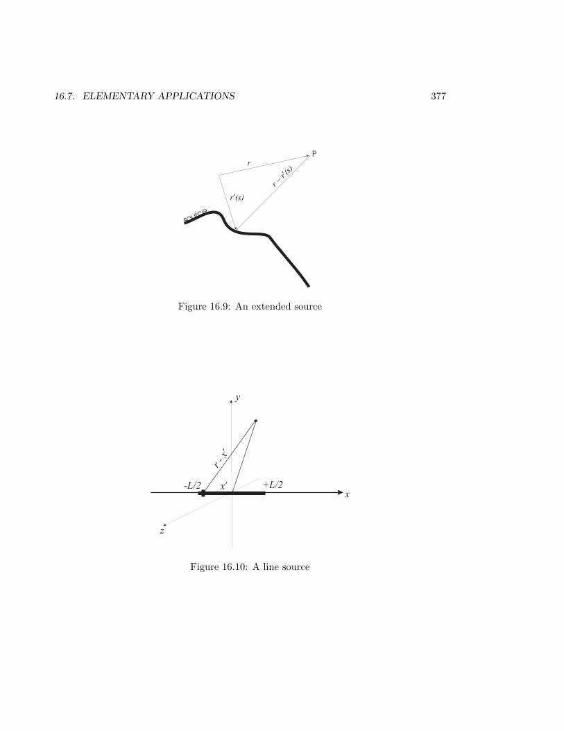
16.7. ELEMENTARY APPLICATIONS 377
P
sourc
e
rr (s
)
-
’
r (s)’
r
Figure 16.9: An extended source
x
y
z
-L/2 +L/2x’
r - x’
Figure 16.10: A line source
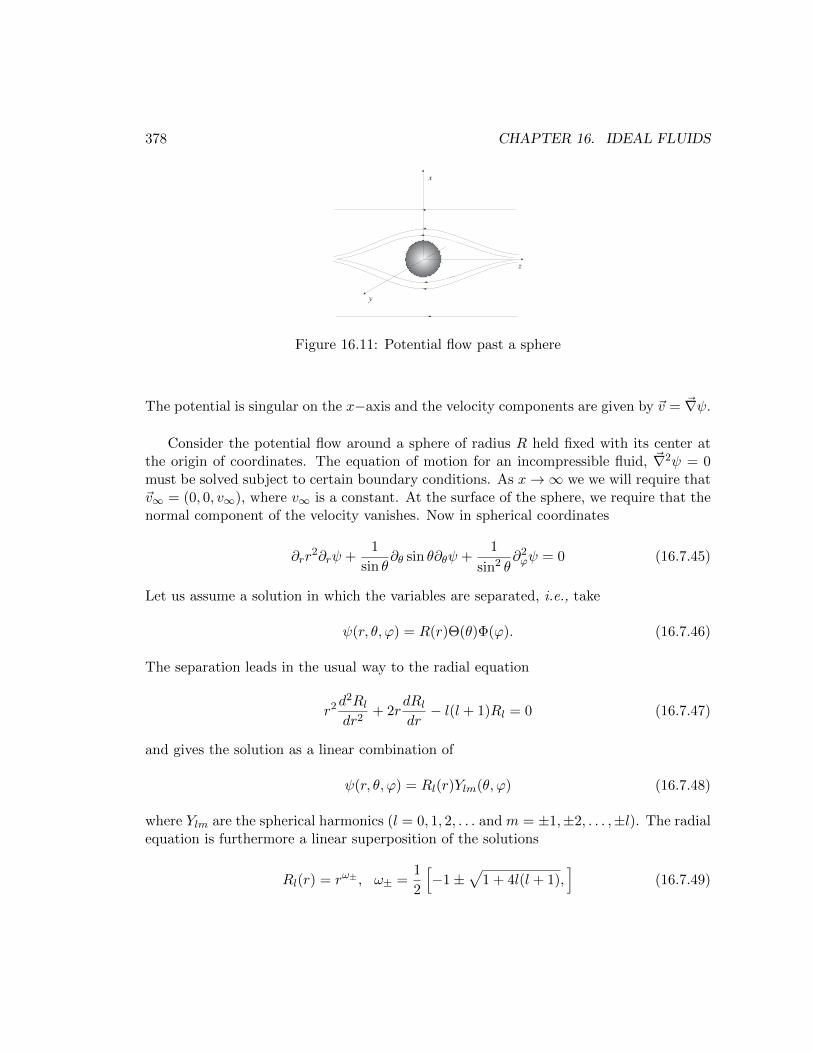
378 CHAPTER 16. IDEAL FLUIDS
z
x
y
Figure 16.11: Potential flow past a sphere
The potential is singular on the x−axis and the velocity components are given by ~v = ~∇ψ.
Consider the potential flow around a sphere of radius R held fixed with its center atthe origin of coordinates. The equation of motion for an incompressible fluid, ~∇2ψ = 0must be solved subject to certain boundary conditions. As x→∞ we we will require that~v∞ = (0, 0, v∞), where v∞ is a constant. At the surface of the sphere, we require that thenormal component of the velocity vanishes. Now in spherical coordinates
∂rr2∂rψ +
1
sin θ∂θ sin θ∂θψ +
1
sin2 θ∂2ϕψ = 0 (16.7.45)
Let us assume a solution in which the variables are separated, i.e., take
ψ(r, θ, ϕ) = R(r)Θ(θ)Φ(ϕ). (16.7.46)
The separation leads in the usual way to the radial equation
r2d2Rldr2
+ 2rdRldr− l(l + 1)Rl = 0 (16.7.47)
and gives the solution as a linear combination of
ψ(r, θ, ϕ) = Rl(r)Ylm(θ, ϕ) (16.7.48)
where Ylm are the spherical harmonics (l = 0, 1, 2, . . . and m = ±1,±2, . . . ,±l). The radialequation is furthermore a linear superposition of the solutions
Rl(r) = rω± , ω± =1
2
[−1±
√1 + 4l(l + 1),
](16.7.49)
16.8. THE CIRCULATION 379
so4
ψ(r, θ, ϕ) = A0 +B0r−1 +(A1r+B1r
−2) cos θ+(A2r2 +B2r
−3)(3 cos2 θ−1)+. . . (16.7.50)
Now if our solution is to reduce to (0, 0, v∞) as r approaches infinity, we should haveA1 = v∞ and Aj = 0 ∀ j ≥ 2. Furthermore, the term B0r
−1 would represent a sphere thatis a source, so we must also set B0 = 0 and, finally, a vanishing radial velocity at r = Ris possible if and only if Bj = 0 ∀ j ≥ 2. We conclude that
ψ(r, θ, ϕ) = A0 + v∞r cos θ +B1r−2 cos θ (16.7.51)
Applying the boundary condition at r = R,
vr(R) = ∂rψ|r=R = 0⇒ v∞ = 2B1R−3 (16.7.52)
we find the solution
ψ(r, θ, ϕ) = v∞
[1 +
R3
2r3
]r cos θ (16.7.53)
which, taking derivatives, gives the velocity field everywhere.
16.8 The Circulation
Define the circulation of a flow, Γ, by the line integral
Γ =
∮C~v · d~r (16.8.1)
about an arbitrary contour drawn in the fluid at some instant. A vortex is a flow in whichthe circulation is non-vanishing in some region. The circulation of an isentropic flow isindependent of time! To prove note that using Euler’s equation we have
dΓ
dt=
∮C
d~v
dt· d~r = −
∮C
~∇pρ· d~r (16.8.2)
and, if the flow is isentropic, ~∇p/ρ = ~∇h⇒
dΓ
dt= −
∮C
~∇h · d~r ≡ 0 (16.8.3)
4Note that
l = 0⇒ ω± = 0,−1l = 1⇒ ω± = 1,−2l = 2⇒ ω± = 2,−3
...
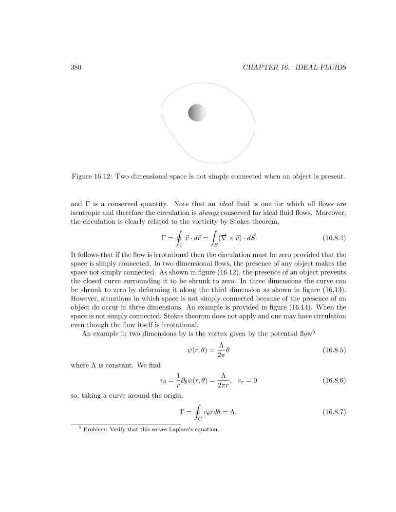
380 CHAPTER 16. IDEAL FLUIDS
Figure 16.12: Two dimensional space is not simply connected when an object is present.
and Γ is a conserved quantity. Note that an ideal fluid is one for which all flows areisentropic and therefore the circulation is always conserved for ideal fluid flows. Moreover,the circulation is clearly related to the vorticity by Stokes theorem,
Γ =
∮C~v · d~r =
∫S
(~∇× ~v) · d~S (16.8.4)
It follows that if the flow is irrotational then the circulation must be zero provided that thespace is simply connected. In two dimensional flows, the presence of any object makes thespace not simply connected. As shown in figure (16.12), the presence of an object preventsthe closed curve surrounding it to be shrunk to zero. In three dimensions the curve canbe shrunk to zero by deforming it along the third dimension as shown in figure (16.13).However, situations in which space is not simply connected because of the presence of anobject do occur in three dimensions. An example is provided in figure (16.14). When thespace is not simply connected, Stokes theorem does not apply and one may have circulationeven though the flow itself is irrotational.
An example in two dimensions by is the vortex given by the potential flow5
ψ(r, θ) =Λ
2πθ (16.8.5)
where Λ is constant. We find
vθ =1
r∂θψ(r, θ) =
Λ
2πr, vr = 0 (16.8.6)
so, taking a curve around the origin,
Γ =
∮Cvθrdθ = Λ, (16.8.7)
5 Problem: Verify that this solves Laplace’s equation.
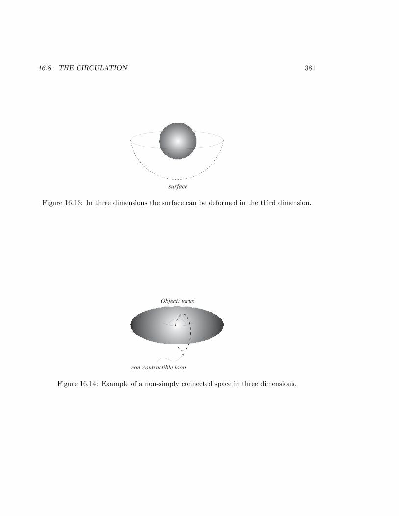
16.8. THE CIRCULATION 381
surface
Figure 16.13: In three dimensions the surface can be deformed in the third dimension.
Object: torus
non-contractible loop
Figure 16.14: Example of a non-simply connected space in three dimensions.
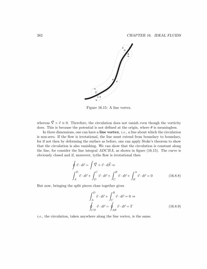
382 CHAPTER 16. IDEAL FLUIDS
D
C
A
B
Figure 16.15: A line vortex.
whereas ~∇× ~v ≡ 0. Therefore, the circulation does not vanish even though the vorticitydoes. This is because the potential is not defined at the origin, where θ is meaningless.
In three dimensions, one can have a line vortex, i.e., a line about which the circulationis non-zero. If the flow is irrotational, the line must extend from boundary to boundary,for if not then by deforming the surface as before, one can apply Stoke’s theorem to showthat the circulation is also vanishing. We can show that the circulation is constant alongthe line, for consider the line integral ADCBA, as shown in figure (16.15). The curve isobviously closed and if, moreover, tythe flow is irrotational then∮
~v · d~r =
∫~∇× ~v · d~S ⇒∫ D
A~v · d~r +
∫ C
D~v · d~r +
∫ B
C~v · d~r +
∫ A
B~v · d~r = 0 (16.8.8)
But now, bringing the split pieces close together gives∫ D
A~v · d~r +
∫ B
C~v · d~r = 0⇒∮
CD~v · d~r =
∮AB
~v · d~r = Γ (16.8.9)
i.e., the circulation, taken anywhere along the line vortex, is the same.
Chapter 17
Energy and Momentum in Fluids
We now turn to the conservation of energy and momentum in fluids. This will lead usto the concept of the stress energy tensor, which will, in turn, serve as our guide as wemove to modify Eulerian dynamics in such a way as to take into account non-ideal fluidsin which energy and momentum is lost by the effects of friction. For incompressible fluids,Euler’s equations will then turn into the Navier-Stokes equations.
17.1 The Energy Flux Density Vector
If u represent the internal energy of a unit mass of fluid and ~v its velocity, then one canwrite the energy per unit volume (or energy density) of fluid as
ε =1
2ρ~v2 + ρu (17.1.1)
and thus its rate of change with time will be
∂ε
∂t=∂ρ
∂t
(1
2~v2 + u
)+ ρ
(~v · ∂~v
∂t+∂u
∂t
)(17.1.2)
Now we can use the equation of continuity to replace ∂ρ/∂t by spatial gradients of thedensity and velocity and we can use the Euler’s equation to do the same with ∂~v/∂t. Whenthis is done, the above equation will take the form
∂ε
∂t= −~∇ · (ρ~v)
(1
2~v2 + u
)− ρ
(~v · (~v · ~∇)~v +
1
ρ~v · ~∇p− ∂u
∂t
). (17.1.3)
However, because
~v · (~v · ~∇)~v =1
2(~v · ~∇)~v2
383
384 CHAPTER 17. ENERGY AND MOMENTUM IN FLUIDS
this may be re-expressed as
∂ε
∂t= −~∇ · (ρ~v)
(1
2~v2 + u
)− ρ
(1
2(~v · ~∇)~v2 +
1
ρ~v · ~∇p− ∂u
∂t
). (17.1.4)
Now apply the first law of thermodynamics to a unit mass of fluid,
du = Tds− pdV = Tds+p
ρ2dρ (17.1.5)
which gives
∂u
∂t= T
∂s
∂t+
p
ρ2
∂ρ
∂t= T
∂s
∂t− p
ρ2~∇ · (ρ~v) (17.1.6)
upon using the equation of continuity. Further,
dh = Tds+dp
ρ⇒ ~∇p = ρ~∇h− ρT ~∇s (17.1.7)
and inserting (17.1.6) and (17.1.7) into the time evolution equation for the energy density,we find
∂ε
∂t= −~∇ · (ρ~v)
(1
2~v2 + u+
p
ρ
)− ρ~v · ~∇
(1
2~v2 + h
)(17.1.8)
and, since h = u+ p/ρ,
∂ε
∂t= −~∇ · (ρ~v)
(1
2~v2 + h
)− ρ~v · ~∇
(1
2~v2 + h
)= −~∇ ·
(ρ~v
[1
2~v2 + h
])(17.1.9)
and integrating both sides over a volume of the fluid enclosed by a surface S, we find usingGauss’ law,
d
dt
∫d3~r ε(t, ~r) = −
∮Sρ~v
[1
2~v2 + h
]· d~S (17.1.10)
The left hand side of the equation represents the change of energy of the volume V , sothe right hand side must represent the energy flux density across the bounding surface S.Thus we call
~E = ρ~v
[1
2~v2 + h
](17.1.11)
the energy flux density vector of the flow.
17.2. MOMENTUM FLUX DENSITY TENSOR 385
17.2 Momentum Flux Density Tensor
Let us follow the same procedure we applied to the energy density, now applying it to themomentum density, which can be defined as ~P = ρ~v. Its time rate of change will obey
∂ ~P
∂t=∂ρ
∂t~v + ρ
∂~v
∂t(17.2.1)
and, using the continuity equation together with Euler’s equations we find
∂ ~P
∂t= −~∇ · (ρ~v)~v − ρ(~v · ~∇)~v − ~∇p (17.2.2)
It is better to rewrite this equation in components as follows
∂t ~Pi = −∂j(ρvj)vi − ρvj∂jvi − ∂ip
= −∂j (ρvivj + pδij) (17.2.3)
and integrating over a volume bounded by the surface S we find
d
dt
∫d3~r Pi = −
∮S
(ρvivj + pδij) dSj (17.2.4)
where we once again used Gauss’ law. As the right hand side represents the rate at whichthe momentum of volume V of the fluid is changing, the right hand side must representthe rate at which momentum is carried enters (or leaves) the volume by flowing into (orout of) the surface S. The tensor
Π(0)ij = pδij + ρvivj (17.2.5)
is the momentum flux density tensor of the flow.
17.3 The Stress Tensor
Let us note that (17.2.3) is just another way to express Euler’s equations. This follows, ofcourse, by symply performing the derivatives,
(∂tρ)vi + ρ(∂tvi) = −∂ip− ρvi∂jvj − ρvj∂jvi − vivj∂jρ (17.3.1)
or, in vector notation,
∂ρ
∂t~v + ρ
∂~v
∂t+ ~∇p+ ρ(~∇ · ~v)~v + ρ(~v · ~∇)~v + (~v · ~∇ρ)~v (17.3.2)
386 CHAPTER 17. ENERGY AND MOMENTUM IN FLUIDS
Now the first term together with the fourth and sixth give the combination[∂ρ
∂t+ ~∇ · (ρ~v)
]~v, (17.3.3)
which vanishes by the continuity equation and we are left with
ρ∂~v
∂t+ ρ(~v · ~∇)~v = −~∇p (17.3.4)
which is simply (16.4.11) in the absence of external forces.
We have considered ideal fluids, i.e., fluids in which there is no energy loss by frictionand no heat transfer either within the fluid or between the fluid and its environment.Unfortunately, the ideal fluid does not exist in nature and it is necessary to think of howEuler’s equations must be modified so as to allow for both of the above possibilities. Oneapproach would be to modify the right hand side of (17.2.3) by adding a term to Πij
Π(0)ij → Πij = pδij + ρvivj − σ′ij
def= ρvivj − σij (17.3.5)
The tensor
σij = σ′ij − pδij (17.3.6)
is called the stress tensor of the fluid and σ′ij is the viscosity tensor. Thus σij givesthe portion of momentum flux that is not due to the direct transfer of momentum withthe fluid mass.
The viscosity tensor must be obtained phenomenologically.
• First we note that internal friction between the molecules will occur when there isan average relative velocity between different portions of the fluid, specifically when∂ivj 6= 0.
• Next, if the velocity gradients are not too large we may suppose that the effects ofviscosity depend only linearly upon them.
• Thirdly, all terms in the viscosity tensor must depend on velocity gradients, and
• finally, the stress tensor must vanish when the fluid as a whole rotates, i.e., when ~vis given as ~v = ~ω × ~r.
For a velocity flow whose components are of the form vi = [~ω× ~r]i = εilmωlxm, its spatialgradients would be ∂jvi = −εijlωl, which is antisymmetric in (i, j). Therefore the sum
λij = ∂jvi + ∂ivj (17.3.7)
17.3. THE STRESS TENSOR 387
vanishes identically and a viscosity tensor defined as
σ′ij = aλij + bδij∂kvk (17.3.8)
would satisfy all the stated conditions. We write the stress tensor as
σij = −pδij + ξ(~∇ · ~v)δij + η
(∂jvi + ∂ivj −
2
3(~∇ · ~v)δij
)(17.3.9)
after rearranging terms and redefining constants so that the term proportional to η istraceless. The coefficients η and ξ could in principle depend on position within the fluid,but we will take them to be constant. η is called the shear viscosity and ξ the bulkviscosity. Now putting everything together,
Πij = pδij + ρvivj − ξ(~∇ · ~v)δij − η(∂jvi + ∂ivj −
2
3(~∇ · ~v)δij
)(17.3.10)
and the modified Euler equations now read
∂t(ρvi) + ∂jΠij = 0, (17.3.11)
which, in the more traditional form, reads
ρ∂~v
∂t+ ρ(~v · ~∇)~v = −~∇p+ η~∇2~v +
(ξ +
η
3
)~∇(~∇ · ~v). (17.3.12)
If the fluid is incompressible so that ~∇ · ~v = 0,
ρ∂~v
∂t+ ρ(~v · ~∇)~v = −~∇p+ η~∇2~v. (17.3.13)
External forces may be taken into account by adding ~f ext to the right hand side of thisequation,
ρ∂~v
∂t+ ρ(~v · ~∇)~v = −~∇p+ η~∇2~v + ~f ext. (17.3.14)
These are the Navier-Stokes equation for an incompressible fluid, a very good approxi-mation when working with liquids to the extent that they can be treated as incompressible,but not so good for gases. On the other hand, for gases the shear viscosity can often beso low as to be negligible and only the bulk term survives. Sometimes the ratio η/ρ isdenoted by ν and called the kinematic viscosity, as opposed to “dynamic” or “absolute”viscosity.
The equation may be reformulated in terms of the vorticity directly if we take the curlof (17.3.14),
ρ∂~ω
∂t+ ρ~∇× (~v · ~∇)~v = η~∇× ~∇2~v + ~∇× ~f ext. (17.3.15)
388 CHAPTER 17. ENERGY AND MOMENTUM IN FLUIDS
Then using
~v × (~∇× ~v) =1
2~∇~v2 − (~v · ~∇)~v, (17.3.16)
we see that~∇× (~v · ~∇)~v = −~∇× (~v × (~∇× ~v)) = −~∇× (~v × ~ω) (17.3.17)
and therefore
ρ∂~ω
∂t− ρ~∇× (~v × ~ω) = η~∇2~ω + ~∇× ~f ext, (17.3.18)
which is the desired equation.
17.4 Energy Dissipation
Because of the viscosity, a flowing fluid will eventually lose its mechanical energy to thermalenergy. For a fixed volume, V , of the fluid the kinetic energy content may be given as
K =1
2
∫Vd3~rρ~v2 (17.4.1)
so we consider the kinetic energy density, k = ρ~v2/2 and its time derivative, assumingthat the fluid density is constant throughout,
∂k
∂t= ρ~v · ∂~v
∂t. (17.4.2)
Then using the Navier-Stokes equation we find
∂k
∂t= ρ~v ·
[−(~v · ~∇)~v −
~∇pρ
+ ν ~∇2~v
], (17.4.3)
which may be put in the form ((~v · ~∇)~v = 12~∇~v2)
∂k
∂t= −ρ~v · ~∇
(1
2~v2 +
p
ρ
)+ η~v · ~∇2~v (17.4.4)
or, using the condition for incompressibility, ~∇ · ~v = 0,
∂k
∂t= −~∇ ·
(1
2ρ~v2 + p
)~v + η~v · ~∇2~v. (17.4.5)
It’s worth examining the last term a bit more. Since ~v · ~∇2~v = vi∂2j vi, consider
1
2∂2j~v
2 = ∂j(vi∂jvi) = vi∂2j vi + (∂jvi)
2 (17.4.6)
17.5. BOUNDARY CONDITIONS 389
and so
~v · ~∇2~v =1
2~∇2~v2 − (∂jvi)
2
⇒ ∂k
∂t= −~∇ ·
[(1
2ρ~v2 + p
)~v − 1
2η~∇~v2
]− η(∂jvi)
2 (17.4.7)
Integrating over the volume, V ,
dK
dt= −
∫ [(1
2ρ~v2 + p
)~v − 1
2η~∇~v2
]· d~S − η
∫Vd3~r (∂jvi)
2 (17.4.8)
The first term represents an energy flux across the bounding surface. It is made up of twoparts, the first corresponding to that of an ideal fluid and the second proportional to ηand representing the flux due to processes of internal friction. The last term representsthe rate of decrease in kinetic energy due to dissipation. If the integral is extended overthe entire volume of the fluid then the surface integral vanishes and we see that the rateof change of total kinetic energy is just
dK
dt= −η
∫Vd3~r (∂ivj)
2 (17.4.9)
17.5 Boundary Conditions
Ideal fluids are required to satisfy the requirement that the normal component of thevelocity field vanishes at the boundaries. For real fluids, depending on the situationencountered, various other conditions may be appropriate. The most common of these arethe following
• No-slip walls: If a boundary is rigid and if the forces between the molecules ofthe fluid and the molecules of the walls of the boundary are strong enough to stopthe tangential motion of the fluid molecules closest to the walls then not only is thenormal component of the velocity field vanishing but also its tangential component,assuming that the boundary is static. The two components (normal and tangential)can only vanish if the velocity itself vanishes at the boundary, i.e., for a real fluid~v = 0 at the (static) boundaries. More generally, if such a “sticky boundary” moveswith a velocity ~u then the fluid velocity would equal ~u at the boundary in this case.Rigid, “sticky” boundaries are called “no-slip” walls.
• Fluid-Fluid interface: To motivate the boundary conditions at the interface oftwo immiscible fluids (eg., oil and water) it is worth asking what force is exerted
390 CHAPTER 17. ENERGY AND MOMENTUM IN FLUIDS
by a fluid (assumed incompressible) on its boundary. If S represents the boundingsurface, the total force will be
Fi =
∮S
ΠikdSk (17.5.1)
so that the force per unit area on the boundary is
fi = Πiknk,= ρ(n · ~v)vi − σiknk, (17.5.2)
where n is the outgoing normal to the surface. If in addition the fluid velocityvanishes at the boundary then the only contribution to the force per unit area comesfrom the second term above,
fi = −σiknk = pni − σ′iknk. (17.5.3)
The first term on the right hand side is the fluid pressure and acts normal to thesurface. The second term, due to viscosity, is the force of friction acting on thesurface. Now, another condition that should be met at the interface is Newton’sthird law of action and reaction, in other words, the force per unit area due to onefluid should exactly balance out the force per unit area due to the other, or
n(1)k σ
(1)ik + n
(2)k σ
(2)ik = 0 (17.5.4)
where n(1,2)k are the unit outgoing normals for the two fluids, labeled by (1) and (2)
and satisfy n(1)i = −n(2)
i .
• Free boundaries: If one of the fluids is inviscid (η = 0), or if the boundary is afree surface of the fluid, shear cannot be supported and we must require the stressto vanish there. This is the condition that
pni − σ′iknk = 0, (17.5.5)
at a free boundary, where nk is the (outgoing) normal.
17.6 Reynolds and Froude Numbers
It is worthwhile reconsidering the significance of each term in the Navier-Stokes equation,
ρ∂~v
∂t+ ρ(~v · ~∇)~v = −~∇p+ η~∇2~v + ~f ext. (17.6.1)
17.6. REYNOLDS AND FROUDE NUMBERS 391
Beginning with the left hand side, the first term defines a “local” acceleration of the fluidand the second a “convective” acceleration depending, as it does, on the spatial change inthe velocity field. Combined the two terms form the “total” derivative
d~v
dt=∂~v
∂t+ (~v · ~∇)~v (17.6.2)
in terms of which the Navier-Stokes equations is sometimes written as
ρd~v
dt= −~∇p+ η~∇2~v + ~f ext. (17.6.3)
The first term on the right hand side represents a normal surface force due to pressure. Thesecond term is the “viscous” force and is of great importance, being the single propertyunique to the concept of a “flow” and therefore to fluids. We have already seen thatviscosity is connected with a transport of momentum between adjoining layers of a fluid,moving at different velocities and that because of it a viscous fluid dissipates energy at arate that is proportional to η, according to (17.4.9). The interaction between adjoininglayers in a fluid arises either (i) because of the intermolecular forces (which are weak ingases) or (ii) by thermal agitation that causes diffusion of molecules from faster movinglayers to slower moving ones. In either case the net result is that mechanical energy isdissipated in the fluid and ends up reappearing as thermal energy. As a result, the flow ofreal fluids is never isentropic – the entropy rises – and always results in the loss of usableenergy. Therefore external forces are always required to maintain fluid motion.
We have five non-linear, coupled differential equations viz., the Navier-Stokes equationsabove, the continuity equation and an equation of state, with which to determine the flowvelocity, the pressure and the density. This is an extremely difficult system to solve andtherefore not many exact solutions are actually available (we will obtain the simplest ofthem here). However, progress in understanding the physical properties of solutions canbe made by some fairly simple considerations based in dimensional analysis.
Now every set of equations will involve a set of variables and a set of parameters, andthese will, in general, be dimensionful. For instance, the independent variables appearingin the Navier-Stokes equations are ~r and t, having mechanical dimensions of length andtime respectively. The mechanical dimension of the dependent variables are
[~v] =l
t, [ρ] =
m
l3, [p] =
m
lt2(17.6.4)
and the mechanical dimension of the viscosity coefficient is
[η] =m
lt. (17.6.5)
(There may be other parameters present in the external force, eg. the acceleration due togravity or Newton’s universal constant of gravitation).
392 CHAPTER 17. ENERGY AND MOMENTUM IN FLUIDS
As in any mechanical system, the number of fundamental physical quantities or di-mensions is three, viz., mass, length and time. We would like to have “typical” valuesfor these quantities, that is, values that characterize the system we are studying. Whatis “typical” would depend on the system of course; for example, if the problem is flowthrough a pipe then we may want to set the “typical” length scale to be the diameteror radius, R, of the pipe. While the length scale is often obvious from the geometry andsymmetries of a given problem, it is difficult to determine a time scale directly. Insteadone picks a “typical” or characteristic velocity scale. Thus, continuing with the exampleof flow in a pipe, we may take the “centerline velocity” i.e., the speed in the center of thepipe, vc, to set the velocity scale. Having a length scale and a velocity scale implies thatwe have a time scale according to
tc = R/vc, (17.6.6)
but what are we to do about a “mass” scale? We will deal with this indirectly as before:if we had a characteristic pressure, pc, instead, then a characteristic mass would be (fromdimensional analysis)
mc = pcRt2c =
pcR3
v2c
(17.6.7)
and a characteristic density,
ρc =mc
R3=pcv2c
, (17.6.8)
Now let’s define the dimensionless quantities
τ =t
tc, ~R =
~r
R, ~u =
~v
vc, ℘ =
p
pc, % =
ρ
ρc(17.6.9)
and re-express the Navier-Stokes equations in terms of them. We find
%d~u
dτ= −∇℘+
ηvcpcR∇2~u (17.6.10)
where ∇ is the gradient operator defined with respect to the scaled, dimensionless coordi-nates and
d~u
dτ=∂~u
∂τ+ (~u · ∇)~u. (17.6.11)
The dimensionless quantity
R =pcR
ηvc(17.6.12)
is called the Reynolds number of the flow. It is sometimes expressed in terms of thekinematic viscosity, ν, as
R =Rvcν, (17.6.13)
17.6. REYNOLDS AND FROUDE NUMBERS 393
where we used the relation ρcv2c = pc and the fact that ~u is defined to be η/ρc. All solutions
will now depend on the dimensionless independent variables and this single dimensionlessparameter, i.e., in particular, ~u = ~u(~R, τ,R), ℘ = ℘(~R, τ,R) and % = %(~R, τ,R). Hadwe included an external force term of the form ~f ext = ρ~g, describing a fluid in a constantgravitational field, then we would find another dimensionless parameter, 1
F =vc√gR
, (17.6.14)
which is called the Froude number and we find
%d~u
dτ= −∇℘+
1
R∇2~u− 1
F2% g (17.6.15)
where g is the unit vector pointing in the direction of ~g. The Reynolds number is relevantonly for viscous flows whereas the Froude number is relevant only for flows occurring ina (constant) gravitational field. In general, in any particular problem, if a length scaleL and a velocity scale V can be identified then the Reynolds and Froude numbers arerespectively
R =V L
νand F =
V√gL
. (17.6.16)
All solutions of the Navier-Stokes equations would depend on the geometry, the boundaryand initial conditions and these two dimensionless parameters. In particular, two systemshaving the same geometry, obeying the same boundary conditions and possessing identicalReynolds and Froude numbers would possess identical scaled velocity, pressure and densityfields and therefore behave identically, their actual velocity fields, pressures and densitydiffering only in scale from one another. Such flows are said to be similar and this is calledthe law of similarity.
So what do the Reynolds number and the Froude number tell us and how are we tointerpret them? Consider the Reynolds number and notice that it is proportional to thecharacteristic speed and length scales but inversely proportional to the kinematic viscosity.Now suppose we wish to test out a new design for an airplane wing with the help of a “windtunnel”. Of course we will want to scale down the wing so that it may fit into our windtunnel, so we construct a smaller but geometrically similar model of the real airplane wing.However, scaling down the wing (i.e., decreasing the characteristic length, L) will lead toa different behavior from the one that describes the real wing unless we keep R the same.Therefore, to truly replicate the behavior of the original wing, the scaling down of the wingspan must be accompanied by a scaling up of the ratio V/ν. This can be accomplished(i) by increasing the characteristic flow speed in the wind tunnel commensurately, whilekeeping the kinematic viscosity the same or (ii) decreasing the kinematic viscosity while
1Problem: Show this and check that F is indeed dimensionless.
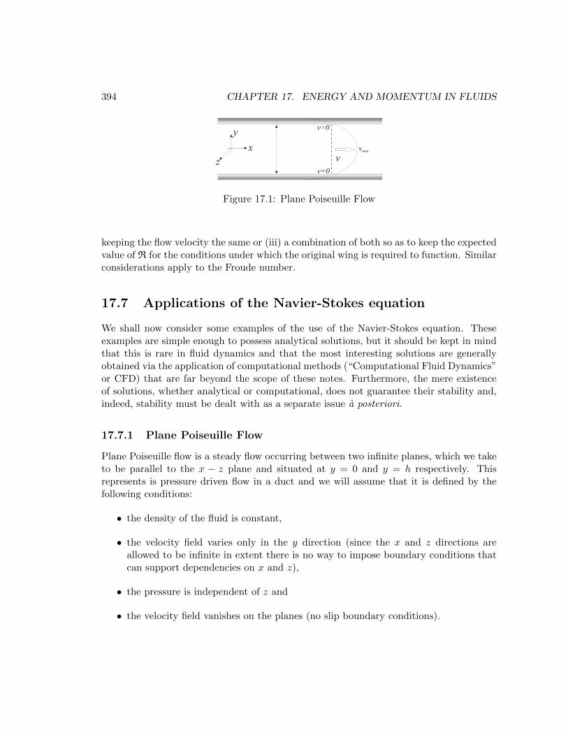
394 CHAPTER 17. ENERGY AND MOMENTUM IN FLUIDS
x
z
y
v
v=0
vmax
v=0
Figure 17.1: Plane Poiseuille Flow
keeping the flow velocity the same or (iii) a combination of both so as to keep the expectedvalue of R for the conditions under which the original wing is required to function. Similarconsiderations apply to the Froude number.
17.7 Applications of the Navier-Stokes equation
We shall now consider some examples of the use of the Navier-Stokes equation. Theseexamples are simple enough to possess analytical solutions, but it should be kept in mindthat this is rare in fluid dynamics and that the most interesting solutions are generallyobtained via the application of computational methods (“Computational Fluid Dynamics”or CFD) that are far beyond the scope of these notes. Furthermore, the mere existenceof solutions, whether analytical or computational, does not guarantee their stability and,indeed, stability must be dealt with as a separate issue a posteriori.
17.7.1 Plane Poiseuille Flow
Plane Poiseuille flow is a steady flow occurring between two infinite planes, which we taketo be parallel to the x − z plane and situated at y = 0 and y = h respectively. Thisrepresents is pressure driven flow in a duct and we will assume that it is defined by thefollowing conditions:
• the density of the fluid is constant,
• the velocity field varies only in the y direction (since the x and z directions areallowed to be infinite in extent there is no way to impose boundary conditions thatcan support dependencies on x and z),
• the pressure is independent of z and
• the velocity field vanishes on the planes (no slip boundary conditions).
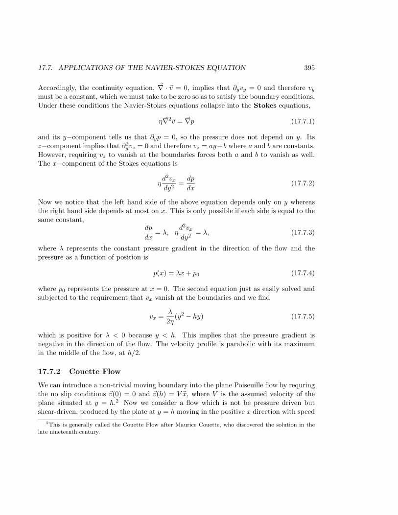
17.7. APPLICATIONS OF THE NAVIER-STOKES EQUATION 395
Accordingly, the continuity equation, ~∇ · ~v = 0, implies that ∂yvy = 0 and therefore vymust be a constant, which we must take to be zero so as to satisfy the boundary conditions.Under these conditions the Navier-Stokes equations collapse into the Stokes equations,
η~∇2~v = ~∇p (17.7.1)
and its y−component tells us that ∂yp = 0, so the pressure does not depend on y. Itsz−component implies that ∂2
yvz = 0 and therefore vz = ay+b where a and b are constants.However, requiring vz to vanish at the boundaries forces both a and b to vanish as well.The x−component of the Stokes equations is
ηd2vxdy2
=dp
dx(17.7.2)
Now we notice that the left hand side of the above equation depends only on y whereasthe right hand side depends at most on x. This is only possible if each side is equal to thesame constant,
dp
dx= λ, η
d2vxdy2
= λ, (17.7.3)
where λ represents the constant pressure gradient in the direction of the flow and thepressure as a function of position is
p(x) = λx+ p0 (17.7.4)
where p0 represents the pressure at x = 0. The second equation just as easily solved andsubjected to the requirement that vx vanish at the boundaries and we find
vx =λ
2η(y2 − hy) (17.7.5)
which is positive for λ < 0 because y < h. This implies that the pressure gradient isnegative in the direction of the flow. The velocity profile is parabolic with its maximumin the middle of the flow, at h/2.
17.7.2 Couette Flow
We can introduce a non-trivial moving boundary into the plane Poiseuille flow by requringthe no slip conditions ~v(0) = 0 and ~v(h) = V x, where V is the assumed velocity of theplane situated at y = h.2 Now we consider a flow which is not be pressure driven butshear-driven, produced by the plate at y = h moving in the positive x direction with speed
2This is generally called the Couette Flow after Maurice Couette, who discovered the solution in thelate nineteenth century.
396 CHAPTER 17. ENERGY AND MOMENTUM IN FLUIDS
x
z
y
V
h
v=V
v=0
Figure 17.2: Couette Flow
V . We will retain all the assumptions of the Poiseuille flow, but one: instead of requiringthat p remain independent only of z we also require that it remain independent of x, sinceboth the x and z directions are of infinite extent and the flow is not driven by the pressure.Once again the continuity equation will require that vy is constant, which can only satisfythe boundary conditions if it vanishes. The y−component of the effective Stokes equationin (17.7.1) then reads ∂yp = 0, which of course implies that p is independent of y as welland therefore it is constant throughout the fluid. The z−component of the same equationyields ∂2
yvz = 0, whose solution, as before, only satisfies the boundary conditions if vz = 0.Finally the x component of the Stokes equation reads
ηd2vxdx2
= 0⇒ vx =V
hy (17.7.6)
is the solution satisfying the no-slip conditions. Here the velocity profile is linear and,not surprisingly, the maximum fluid velocity occurs in the layer adjoining the movingboundary. It is independent of the viscosity. This simple flow is particularly useful in theanalysis of lubrication.
17.7.3 Hagen-Poiseuille Flow
We consider the conditions of the Poiseuille flow, but this time in a cylindrical pipe ofinfinite length and radius R, whose axis we take to be the z−axis. The symmetry makesit most convenient to work in cylindrical coordinates. Thus we take ρ to be constant asbefore, we assume the flow is steady, depending only on the radial coordinate and weimpose no slip boundary conditions, ~v(R) = 0. Moreover, we assume that the pressuredoes not depend on the azimuthal coordinate so that p = p(r, z).
This provides an excellent opportunity to use the methods of Chapter 15. Thus the
17.7. APPLICATIONS OF THE NAVIER-STOKES EQUATION 397
continuity equation reads3
~∇ · ~v = 0 = ∇jvj = ∂jvj + Γjjlv
l (17.7.7)
and using the Christoffel symbols derived in (15.4.16) we find
∂rvr +
vr
r= 0⇒ vr =
a
r, (17.7.8)
which can only vanish because of the boundary conditions. Next, the Navier-Stokes equa-tions read
ρ(~v · ~∇)~v = −~∇p+ η~∇2~v (17.7.9)
which, in components, becomes
ρ(vj∂jvi + Γijkv
jvk) = −gij∂jp+ ηgjk∇j∇kvi (17.7.10)
The first term on the left vanishes because all velocity components depend only r andvr = 0. Thus
gij∂jp = ηgjk∇j∇kvi − ρΓijkvjvk (17.7.11)
This turns into a complicated expression, but it is immensely simplified if we recall thatthe flow velocity may depend only on r. One eventually finds the following equations
∂rp = ρrvϕ2
0 = η
(d2vϕ
dr2+
3
r
dvϕ
dr
)∂zp = η
(d2vz
dr2+
1
r
dvz
dr
)(17.7.12)
The second equation above has the solution
vϕ =a
2
R2 − r2
r2R2(17.7.13)
but, even though it satisfies the boundary conditions, it is ill behaved on the axis and somust be set to zero by taking a = 0. By the first equation of (17.7.12) this means thatthe pressure is a function only of z. The last equation of (17.7.12) can be written as
dp
dz= η
(d2vz
dr2+
1
r
dvz
dr
)= λ (17.7.14)
3We must be careful to distinguish between covariant and contravariant quantitites since we are nowworking in a changing basis.
398 CHAPTER 17. ENERGY AND MOMENTUM IN FLUIDS
where λ is a constant representing the pressure gradient in the the z−direction. Thesolution that obeys the boundary conditions and is well behaved on the axis is
p = λz + p0, vz = vz =λ
4η(r2 −R2) (17.7.15)
The velocity profile, as in the planar case, is parabolic and its maximum is achieved whenr = 0, at which vz,max = −λR2/4η. Blood flow through the arteries, for example, canbe modeled by the Hagen-Poiseuille solution above. The volume of fluid delivered can beshown to be proportional to the fourth power of the pipe radius,4 which means that acondition like arteriosclerosis, which is the accumulation of fatty material on the walls ofthe arteries, can very rapidly block the flow of blood to cells.
17.8 Relativistic Fluids
We have seen that the dynamics of ideal fluids in the absence of external forces is suitablyexpressed by the continuity equation, the three Euler equations,
∂t(ρvi) + ∂jΠ(0)ji = 0, (17.8.1)
where Π(0)ji = pδji + ρvjvi represents the momentum flux density tensor and one equation
of state relating the pressure to the energy density. Clearly, the continuity and Eulerequations are valid only in the regime in which Galilean relativity applies, i.e., when theflow velocity is much less than the speed of light. We seek a generalization of this equationthat is valid even when the flow velocity is close to the speed of light. This essentiallymeans that we want to construct a second rank tensor, Tµν , that reduces to the momentumflux density tensor at low flow velocity. We go about this in the same way as we wentabout deducing the structure of the relativistic force four vector in Chapter 13.
17.8.1 Perfect Fluids
Consider therefore a frame in which the fluid is instantaneously at rest, i.e., vi = 0. Inthis frame Πij = pδij , and we must identify this with the spatial part of T
µν,5 but what
can be said about the temporal part? Since all terms in the trace of T
ηµνTµν
= Tµµ = T
00 + 3p (17.8.2)
4Problem: Compute the total volume of fluid that flows through a cross section of the pipe per second.5We write everything in contravariant form for ease of calculation. In a Cartesian frame there is no
difference between covariant and contravariant three tensors.
17.8. RELATIVISTIC FLUIDS 399
must have the same mechanical dimension, it follows that
[T0
0] = [p] =m
lt2(17.8.3)
and again, because T00
= η00T0
0, the mechanical dimension of T00
must be
[T00
] =m
l3(17.8.4)
Thus we take T00
= ρ, the mass density of the fluid. Finally, because we are in the
instantaneous rest frame we set T0i
= Ti0
= 0 and we get the energy-momentum fluxdensity tensor – or energy-momentum tensor for short – in the instantaneous rest frame,
Tµν
=
ρ 0 0 00 p 0 00 0 p 00 0 0 p
(17.8.5)
To find the energy momentum tensor in an arbitrary frame, we simply perform a Lorentztransformation with boost parameter vi,
Tµν = LµαLνβT
αβ(17.8.6)
and get the expressions
T 00 = L0αL
0βT
αβ= γ2
(ρ+
~v2
c4p
)= − p
c2+(ρ+
p
c2
)γ2
T 0i = L0αL
iβT
αβ= L0
0Li0T
00+ L0
jLikT
jk=(ρ+
p
c2
)γ2vi
T ij = LiαLjβT
αβ= Li0L
j0T
00+ LimL
jnT
mn= pδij +
(ρ+
p
c2
)γ2vivj
(17.8.7)
where we have used the expressions in (14.3.42). Recall that U0 = γ and U i = γvi are thecomponents of the four velocity vector as defined in (14.5.15). With these definitions, thecomponents above can be integrated into the single symmetric tensor
Tµν = pηµν +(ρ+
p
c2
)UµUν (17.8.8)
Just as the conservation of fluid momentum yields Euler’s equations for a non-relativisticfluid, so also the motion of the relativistic fluid is governed by energy-momentum conser-vation,
∂µTµν = 0. (17.8.9)
400 CHAPTER 17. ENERGY AND MOMENTUM IN FLUIDS
This is a set of four equations so let’s see what they mean, first in the non-relativisticlimit: we are interested in the limit of small velocities so take U0 = γ ≈ 1 and U i ≈ vi,and find that indeed
T 00 ≈ ρ
T 0i ≈ ρvi
T ij ≈ pδij + ρvivj (17.8.10)
where we have taken c → ∞. The time component of the conservation of energy andmomentum then gives in this limit
∂tT00 + ∂iT
i0 = 0 = ∂tρ+ ∂i(ρvi) (17.8.11)
or, in vector form,∂ρ
∂t+ ~∇ · (ρ~v) = 0, (17.8.12)
which we recognize as the continuity equation. Likewise the space components of theequation yield
∂tT0i + ∂jT
ji = 0 = ∂t(ρvi) + ∂ip+ ∂j(ρv
ivj) (17.8.13)
This can be rewritten as
(∂tρ)vi + ρ∂tvi + ∂ip+ ∂j(ρv
j)vi + ρvj∂jvi = 0 (17.8.14)
and, using the continuity equation above, it can be expressed in vector form as
ρ∂~v
∂t+ ρ(~v · ~∇)~v = −~∇p, (17.8.15)
which, of course, are Euler’s equations.Energy and momentum conservation yields more complicated equations at high flow
velocities. The continuity equation in vector form is now
∂
∂t
(p~v2/c4 + ρ
1− ~v2/c2
)+ ~∇ ·
((p/c2 + ρ)~v
1− ~v2/c2
)= 0 (17.8.16)
and, using this condition, the relativistic Euler equations get simplified to6
∂~v
∂t+ (~v · ~∇)~v = −1− ~v2/c2
p/c2 + ρ
[~∇p+
v
c2
∂p
∂t
](17.8.17)
6To arrive at the Euler equations from energy momentum conservation, begin with the space componentsof the conservation law,
∂t[( pc2
+ ρ)γ2vi
]+ ∂j
[pδji +
( pc2
+ ρ)γ2vjvi
]= 0
17.8. RELATIVISTIC FLUIDS 401
17.8.2 Conserved Currents
A fluid may carry other conserved quantities (such as electric charge) besides energy andmomentum, so what does the conservation law for such quantities look like? In this section,we address this question for conserved scalars. Let A be one such conserved quantity andlet a represent its comoving density, i.e., its density in a frame that moves with the fluidat each point (the comoving frame). We define a current density, Aµ, associated with thisquantity, by requiring it to have the form
A0
= a, Ai
= 0 (17.8.18)
in the comoving frame. In any other frame, its form will be given by a boost
A0 = L00A
0= γa, Ai = Li0A
0= γavi (17.8.19)
or, more concisely, Aµ = aUµ. The statement that the quantity whose comoving density is“a” is conserved is then equivalent to the Lorentz covariant statement that the associatedcurrent density is divergence free,
∂µAµ = 0. (17.8.20)
This equation generalizes (16.2.4). It can be put into integral form if we integrate theequation over a volume V bounded by the surface S,∫
Vd3~r∂µA
µ =d
dt
∫Vd3~rA0 +
∫Vd3~r ~∇ · ~A, (17.8.21)
and use Gauss’ theorem for the second term on the right to get
d
dt
∫Vd3~rA0 = −
∮S
~A · d~S, (17.8.22)
which is a generalization of (16.2.2).For example, if the total number, N , of fluid particles in a given volume is conserved,
let n represent the number density of particles. The conservation of particle number can
Expanding and collecting terms, it is straightforward to put this equation in the form
∂t~v + (~v · ~∇)~v = −1− ~v2/c2
p/c2 + ρ
[~∇p+ ~v
(∂t
[(p/c2 + ρ)
1− ~v2/c2
]+ ~∇ ·
[(p/c2 + ρ)~v
1− ~v2/c2
])]Now
p~v2/c2 + ρ = (p/c2 + ρ)− p/(γ2c2)⇒ (p/c2 + ρ)γ2 = (p~v2/c2 + ρ)γ2 + p/c2
and so∂t[(p/c
2 + ρ)γ2] = ∂t[(p~v2/c2 + ρ)γ2] + 1/c2∂tp
Problem: Complete the steps leading to the Euler equations.
402 CHAPTER 17. ENERGY AND MOMENTUM IN FLUIDS
be expressed as the statement that the number density current, Nµ = nUµ is divergencefree,
∂µ(nUµ) = 0. (17.8.23)
If the fluid is charged then, lettingN+ represent that number of positively charged particlesand N− the number of negatively charged particles, conservation of charge would requirethat N+ − N− remains constant throughout the motion. We can construct the chargedensity, ρq = q(n+−n−), where q is the magnitude of the elementary charge, and the chargecurrent density, jµq = ρqU
µ. Conservation of charge is then embodied in the requirementthat ∂µj
µq = 0.
The conservation of energy and momentum together with the conservation of particlenumber leads naturally to the second law of thermodynamics as we now show. Energy-momentum conservation requires that
Uβ(∂αTαβ) = 0 = Uβ
[∂βp+ ∂α
( pc2
+ ρ)UαUβ
](17.8.24)
and, using UβUβ = −c2, we may re-express this in the form
Uβ∂βp− ∂β[(p+ ρc2)Uβ] = 0 (17.8.25)
or− U · ∂(ρc2)− (p+ ρc2)∂ · U = 0 (17.8.26)
but, if the particle number is also conserved, then
∂β(nUβ) = 0⇒ ∂ · U =U · ∂nn
(17.8.27)
and, inserting this relation into (17.8.26), we find
U ·[−∂(ρc2) +
1
np∂n+
ρc2
n∂n
]= 0 (17.8.28)
and therefore
− nU ·[p∂
(1
n
)+ ∂
(ρc2
n
)]= 0 (17.8.29)
or
pd
(1
n
)+ d
(ρc2
n
)= 0. (17.8.30)
Now 1/n is simply the specific volume, v, or the volume per particle of the fluid and ρc2/nis the energy per particle, which we call ε, so the conservation of energy, momentum andparticle number for a perfect fluid imply the relation
dε+ pdv = 0. (17.8.31)
17.8. RELATIVISTIC FLUIDS 403
This has the form of the first law of thermodynamics,
Tdσ = dε+ pdv, (17.8.32)
where σ represents the specific entropy (or entropy per particle) and says that the flow isisentropic, i.e., dσ = 0. Since nσ represents the comoving entropy density of the fluid, wecan form the entropy current four vector Sµ = nσUµ, which is conserved during the flow.
17.8.3 Imperfect Fluids
The energy momentum tensor describing non-ideal fluids must include terms involving theshear and bulk viscosity. We assume that these terms add to the stress energy tensor andcollect all of them in the tensor ∆Tµν writing
Tµν = Tµν(0) + ∆Tµν (17.8.33)
where T(0)µν represents the ideal fluid tensor and ∆Tµν purports to contain the effects of
dissipation. Likewise, for the number density current we write
Nµ = Nµ(0) + ∆Nµ = nUµ + ∆Nµ, (17.8.34)
where ∆Nµ represents the particle drift. However, correction terms of this kind introducean ambiguity in the definition of the fluid four velocity because heat transfer makes itnecessary to specify whether Uµ represents the four velocity of energy transport (theenergy frame) or of particle transport (the particle frame).7
Before commiting ourselves to a particular frame and considering what specific form∆Tµν might take, let’s examine some of the consequences of dissipation. As before, energyconservation and the balance equation for the particle number will take the form8
∂αTαβ = 0 = ∂αN
α (17.8.35)
Following the same steps as for a perfect fluid, energy momentum conservation is seen torequire that
Uβ(∂αTαβ) = −nU ·
[p∂
(1
n
)+ ∂
(ρc2
n
)]+p+ ρc2
n∂ ·∆N + Uβ∂α∆Tαβ = 0 (17.8.36)
7The energy frame is attributed to Landau and Lifshitz, Fluid Mechanics, 2nd ed., Pergamon Press, NY(1987), and the particle frame is attributed to Eckart, Phys. Rev. D 58 (1940) 919.
8Here, we will always assume that there are no external sources or sinks and no particle creationor annihilation by chemical processes within the fluid. If this does not hold then the particle numberconservation law must be modified by the addition of a term which allows for a change in the fluidcomposition,
∂αNα = Ψ.
404 CHAPTER 17. ENERGY AND MOMENTUM IN FLUIDS
Now the first term is given in terms of the specific entropy according to the first law ofthermodynamics, so
− TnUµ∂µσ +p+ ρc2
n∂ ·∆N + Uν∂µ∆Tµν = 0 (17.8.37)
and using the conservation of particle number, ∂α(nUα + ∆Nα) = 0, we find
∂µ(nσUµ) =µ
T∂ ·∆N +
1
TUν∂µ∆Tµν . (17.8.38)
where
µ =
(p+ ρc2
n− σT
)(17.8.39)
is Euler’s relation. In the absence of the dissipation terms we had identified Sµ = nσUµ
as the entropy current four vector but (17.8.38) says that when dissipation is present thiscurrent is not conserved. This is to be expected in the presence of dissipation, so letus evaluate the right hand side of this equation. If we continue to interpret ρ and n asthe energy density and particle number density respectively in the comoving frame, then
∆T00
= 0 = ∆N0. With this interpretation, evaluating the right hand side of (17.8.38) in
the comoving frame9 we find
∂µ(nσUµ) =µ
T∂i∆N
i − c2
T∂i∆T
i0, (17.8.40)
which may be negative for arbitrary flows and could violate the second law of thermody-namics if we continued to interpret Sµ = nσUµ as the entropy current four vector. This isnot surprising since we must allow for the possibility that Sµ is modified by the dissipationterms.
How then should the entropy current four vector be defined? One proceeds as follows:first define Sµ so that (i) its divergence contains no gradients of ∆Tµν and (ii) the entropy
density is S0
= nσ in the local rest frame, then (iii) determine ∆Tµν and ∆Nµ byrequiring that the divergence of the entropy current is non-negative in any process. Thelast condition is justified by the second law of thermodynamics and can be accomplishedby setting
Sµ = nσUµ − µ
T∆Nµ − 1
TUν∆Tµν , (17.8.41)
which leads to
∂µSµ = −∂µ
(µT
)∆Nµ − ∂µ
(UνT
)∆Tµν . (17.8.42)
9It is most straightforwardly evaluated in a comoving frame. Because we are evaluating a scalar weexpect that the result will hold in any frame.
17.9. SCALING BEHAVIOR OF FLUID FLOWS 405
We take (17.8.41) as a definition of the entropy current and determine ∆Tµν by requiringthat its divergence never decreases for any flow. Then (17.8.42) gives the rate of entropyproduction per unit volume in the presence of dissipation.
Now we must address the question of what form ∆Nµ and ∆Tµν can take. Since wehave required ∂µS
µ to be non-negative, let us expand the right hand side of (17.8.42) ina local comoving frame, keeping in mind our interpretation of n and ρ and setting U i andall gradients of U0 equal to zero,10
∂µSµ = −∂i
(µT
)∆N
i −(
1
TUi +
c2
T 2∂iT
)∆T
i0 − 1
T(∂iUj)∆T
ij(17.8.43)
In order for the right hand side to be non-negative for all fluid configurations each termmust be a perfect square. This leads to
∆Ni
= −αηij (T∂jµ− µ∂jT ) ,
∆Ti0
= ∆T0i
= −χ(T U i + c2ηij∂jT
)(17.8.44)
and
∆T ij = −η(∂iUj + ∂jUi −
2
3(∂ · U)ηij
)− ξ(∂ · U)ηij (17.8.45)
where α, χ, η and ξ are non-negative, possibly temperature dependent, coefficients. Bydirect comparison with the non-relativistic momentum flow tensor we immediately identifyη and ξ with the shear and bulk viscosity coefficients respectively. The new quantities arethe diffusion coefficient, α, and the coefficient of heat conduction, χ.11
17.9 Scaling behavior of fluid flows
A class of particular solutions to the Hydrodynamic equations have the form f(~r, t) =g(t)F [~r/h(t)], where g(t) and h(t) are time dependent scales of the spatial coordinate andf(~r, t) is any of the unknown functions appearing in the Navier-Stokes equations. Suchsolutions are called self-similar because the spatial distribution of these solutions remainssimilar to itself at all times during the motion.
10Problem: Show this.11The distinction between the Eckart and Landau-Lifshitz pictures arises as follows: If Uµ is taken to be
the velocity of particle transport (Eckart) then comoving observers do not see any particle drift, ∆Nµ
= 0,which implies that the diffusion coefficient vanishes. If Uµ is taken to be the velocity of energy transport(Landau and Lifshitz) then comoving observers do not observe any contribution to the energy flux, so
∆T0µ
= 0, i.e., the coefficient of heat conduction must vanish.
406 CHAPTER 17. ENERGY AND MOMENTUM IN FLUIDS
To understand how such solutions come about, let us return to the non-relativisticNavier-Stokes equation in (17.3.14) and ask how the variables and parameters behaveunder a multiplicative change in the spatial and temporal scales,
~r → ~r′ = σ~r
t→ t′ = σαt (17.9.1)
where σ is the “scale factor”. The scaling dimension of a variable or parameter is thepower of σ in the transformation
f → f ′ = σbf. (17.9.2)
Thus ~r has scaling dimension unity and t has scaling dimension α. If the Navier-Stokesequation is to be scale invariant then all terms in the equation must have the same scalingdimension. Dividing throughout by ρ we find that for the two terms on the left hand sideof the equation to have the same scaling dimension the velocity must scale as
~v → ~v′ = σ1−α~v (17.9.3)
and the scaling dimension of the left hand side becomes 1− 2α. This requires p/ρ to havescaling dimension 2(1 − α) and the kinematic viscosity to have scaling dimension 2 − α,i.e.,
p/ρ→ p′/ρ′ = σ2(1−α)p/ρ
ν → ν ′ = σ2−αν (17.9.4)
Suppose that the viscosity has scaling dimension β, then we will have the following scalingbehavior for all our variables
~r → ~r′ = σ~r
t→ t′ = σαt
~v → ~v′ = σ1−α~v
η → η′ = σβη
ρ→ ρ′ = σβ+α−2ρ
p→ p′ = σβ−αp (17.9.5)
17.9. SCALING BEHAVIOR OF FLUID FLOWS 407
and we recognize that the Reynolds number remains invariant provided that the charac-teristic values of the parameters and variables that determine R also scale as above.
The self-similarity relations above may be regarded as special cases of a more generalrelation of the form
f(~r, t)→ f(σ~r, σαt) = σbf(~r, t) (17.9.6)
where σ is a function of t. Now we have the following theorem: a necessary and sufficientcondition for a function f(~r, t) to satisfy the above condition is that
f(~r, t) = tb/αF (~r/t1/α) (17.9.7)
That it is necessary follows because if we take σ = t−1/α then
f(σ~r, σαt) = σbf(~r, t)⇒ f(~r/t1/α, 1) = t−b/αf(~r, t)⇒ f(~r, t) = tb/αF (~r/t1/α), (17.9.8)
where F (x) = f(x, 1). Of course, σ is constant in (17.9.5), therefore the condition is notin fact a necessary one in our particular case. However, that it is sufficient even for aconstant scaling parameter is straightforward since
f(~r, t) = tb/αF (~r/t1/α)⇒ f(σ~r, σαt) = σbtb/αF (~r/t1/α) = σbf(~r, t) (17.9.9)
and so, according to (17.9.5), the velocity function
~v(~r, t) = t(1−α)/α~v(~r/t1/α) (17.9.10)
will represent a self-similar flow. We therefore have a one parameter family of self-similarsolutions. For example, the solution with α = 1 will have
~v(~r, t) = ~u(~r/t) (17.9.11)
and with α = 2 we should find
~v(~r, t) =1√t~u(~r/√t). (17.9.12)
Self-similar solutions are interesting from a theoretical point of view because the NavierStokes equations are reduced to ordinary differential equations. However, the equationsobtained are non-linear and so it is often not clear that much by way of simplificationhas in fact been gained. In practical terms these solutions appear to be applicable whenthe effects of boundaries can be ignored or when the boundaries have only a local effectso that in most of the fluid domain the self-similar solution remains valid. This must beverified independently before a given self-similar solution is taken to be relevant to anyreal situation.
408 CHAPTER 17. ENERGY AND MOMENTUM IN FLUIDS
17.10 An Example
Similar arguments can be made for relativistic hydrodynamics as well and we leave that asan exercise for the reader.12 Let us close our discussion of fluid dynamics by consideringa special self-similar solution to the hydrodynamic equations for a relativistic, imperfectfluid, first in two and then in four space-time dimensions. This will serve to put togetherthe concepts of the last two sections in a single problem, which also turns out to bephysically interesting in its own right because it is believed to describe the evolution ofvery hot (ultra-relativistic) hadron matter produced in extreme relativistic nucleus-nucleuscollisions as well as in the very early universe.
The solutions we seek will be of the following form: if qi ∈ 1, 2, 3 compose somearbitrary, orthogonal coordinate system in which hi are the corresponding scale factors sothat
ds2 = c2dt2 − h2i dq
i2, (17.10.1)
then we assume that the velocity along any non-compact dimension is
vi(qi, t) =sihit
(17.10.2)
where si is the spatial distance,
si =
∫hidqi, (17.10.3)
and it is zero along any compact dimension.
We will begin with a two dimensional version of this problem. In order to generatesuch a flow in two dimensions with
ds2 = c2dt2 − dx2 (17.10.4)
and v(x, t) = x/t, we first seek the local comoving frame of the fluid. Let (τ, y) representthe coordinates in this frame, then by definition U τ = 1 and Uy = 0. To determine (τ, y)we simply note that
U τ =∂τ
∂tU t +
∂τ
∂xUx = 1, Uy =
∂τ
∂tU t +
∂τ
∂xUx = 0 (17.10.5)
Now because v(t, x) = x/t
Ux =cx√
c2t2 − x2, U t =
ct√c2t2 − x2
(17.10.6)
12Problem: Repeat the scaling arguments above for the relativistic hydrodynamic equations. Argue thatthe only Lorentz invariant scaling solution has α = 1.
17.10. AN EXAMPLE 409
and it is easy to see that the solutions of the two linear, first order equations for τ and yare
τ =1
c
√c2t2 − x2 + f
(xt
),
y = y(xt
)(17.10.7)
where f and y are arbitrary functions of their argument. Given this coordinate transfor-mation, we can construct the inverse vielbein as follows
Eτt =∂τ
∂t=
ct√c2t2 − x2
− x
t2f ′(x/t)
Eτx =∂τ
∂x= − x
c√c2t2 − x2
+1
tf ′(x/t)
Eyt =∂y
∂t= − x
t2y′(x/t)
Eyx =∂y
∂x=
1
ty′(x/t) (17.10.8)
where the prime refers to a derivative with respect to the argument x/t and we find themetric components in the new system according to
gµν = ηabEµaEνb (17.10.9)
Carrying out the algebra yields
gττ = − 1
c2+c2t2 − x2
c2t4f ′(x/t)2
gτy =c2t2 − x2
c2t4f ′(x/t)y′(x/t)
gyy =c2t2 − x2
c2t4y′(x/t)2 (17.10.10)
Since f and y are arbitrary functions and y is not allowed to vanish, we choose f = 0.This rids us of the off-diagonal component of gµν . We see also that
gyy =τ2
t4y′(x/t)2 ⇒ y′(x/t)2 =
t4
τ2gyy (17.10.11)
and, because y′ must also be a function of x/t, we take gyy = 1/τ2. This gives
y′(v) =t2
τ2=
c2
c2 − v2(17.10.12)
410 CHAPTER 17. ENERGY AND MOMENTUM IN FLUIDS
where v = x/t, along with the solution
y(x/t) = c tanh−1( xct
)+ const. (17.10.13)
y(x/t) is called the “rapidity”.To sumarize our progress so far: for the fluid flow v(t, x) = x/t, we have determined a
comoving frame, in which U τ = 1 and Uy = 0, whose space-time metric is
ds2 = c2dτ2 − τ2dy2. (17.10.14)
In this frame the ideal fluid energy momentum tensor has the form
Tµν =
(ρ 00 p
τ2
)(17.10.15)
and it is a simple matter to solve the Euler equations,
∇µTµτ =∂ρ
∂τ+ρ
τ+
p
c2τ= 0
∇µTµy =∂p
∂y= 0. (17.10.16)
The last equation says that p = p(τ) and the first can only be solved after specifyingequation of state. Let us use the equation of state for an extremely relativistic (flowvelocity close to the speed of light) bosonic fluid, which we know from statistical mechanicsto be
p =1
3ρc2 =
1
3γT 4, (17.10.17)
where T is the fluid temperature and γ is the Stefan-Boltzmann constant. With this,Euler’s equations are solved by
ρ = ρ0
(τ0
τ
)4/3, (17.10.18)
where ρ0 is the mass density at the time τ0, which we understand as the time required toachieve the initial thermal equilibrium. The temperature behavior as a function of τ thenfollows directly.
We’ll now include the effects of dissipation, but take the fluid to be incompressible sothat ξ = 0. Let Uµ represent the velocity of particle transport. To simplify matters stillfurther, suppose also that the temperature dependence of both χ and η are given by thepower laws,
η(T ) = η0Ta
χ(T ) = χ0Tb (17.10.19)
17.10. AN EXAMPLE 411
and that the flow is extremely relativistic so that (17.10.17) holds. The components of thefull energy momentum tensor in our comoving frame are
T 00 = ρ
T 0i = T i0 = −c2χ0T
b
τ2∂yT
T ij =p
τ2− 4η0T
a
3τ3(17.10.20)
where the prime refers to a derivative with respect to y. The conservation equation
∇µTµy = ∂yp−4η0
3τ∂yT
a − χ0c2
[T b
τ∂yT + ∂τ (T b∂yT )
]= 0, (17.10.21)
once again implies that the temperature does not depend on the rapidity, i.e., T = T (τ)and, after dropping all derivatives with respect to the rapidity, the other equation becomes
∇µTµτ = ∂τρ+ρ
τ+
p
c2τ− 4η0T
a
3c2τ2= 0, (17.10.22)
which is seen to be a Bernoulli equation when rewritten in terms of the temperature,
∂τT +T
3τ− η0
3γ
T a−3
τ2= 0. (17.10.23)
It has the solutions
T = T0
(τ0
τ
)1/3exp
[− η0
3γ
(1
τ− 1
τ0
)], if a = 4
T = T0
(τ0
τ
)1/3[1− η0
γ
T−30
τ0ln(τ0
τ
)]1/3
, if a = 1 (17.10.24)
and
T = T0
η0
γ
(a− 4
a− 1
)T a−4
0
τ− (a−1)3 − τ−
(a−1)3
0
τ−(a−4)
3
+(τ0
τ
)−a−43
−1a−4
(17.10.25)
otherwise. Thus there is no energy loss via heat conduction for this type of flow.For completeness, let us also compute the entropy production for this one dimensional
flow. Continuing in the comoving frame we have,
Sτ = nσ, Sy = 0 (17.10.26)
412 CHAPTER 17. ENERGY AND MOMENTUM IN FLUIDS
and (17.8.43), which reduces to
∂τ (nσ) +nσ
τ=
4η0
3
T a−1
τ2. (17.10.27)
Once again we arrive at a Bernoulli equation, this time for the rate of entropy production.With Q(τ) = 4η0T
a−1/3τ2, we find the entropy density to be
S(τ) =τ0
τ
[S(τ0) +
1
τ0
∫ τ
τ0
dτ ′τ ′Q(τ ′)
](17.10.28)
Now the entropy contained in any interval dy will be
dS = S(τ)τdy (17.10.29)
and therefore
∂τ (∂yS) = τQ(τ) (17.10.30)
showing that the rapidity density of the entropy is not a constant of the motion butincreases as a consequence of the dissipation.
Four dimensional expansion with the velocity distribution specified in the introductionto this section may similarly be described in arbitrary, orthogonal frames. An interestingfeature of these solutions is that the effects of dissipation vanish exactly. This is a conse-quence of the velocity distribution and the fact that there are no constraints on the systemdue to external boundaries, hence no shear viscosity. We will consider separately the casesof co-ordinate systems with no compact co-ordinate and one compact co-ordinate.
If none of the co-ordinates are compact (for example Cartesian or parabolic cylindricalco-ordinates) we can generate a self-similar solution for the velocity distribution (17.10.2)in a manner similar to that employed before i.e. by introducing comoving coordinates. Itcan easily be shown that these coordinates are quite generally given by
τ =
√√√√c2t2 −3∑i=1
s2i
u =1
2ln
√c2t2 −
∑2i=1 s
2i + s3√
c2t2 −∑2
i=1 s2i − s3
v =
1
2ln
[√c2t2 − s2
1 + s3√c2t2 − s2
1 − s3
]y =
1
2ln
[ct+ s1
ct− s1
](17.10.31)

17.10. AN EXAMPLE 413
With the same equation of state that we have been using, the temperature will be afunction only of τ and we find a remarkably simple equation for the temperature evolution
∂τ ε+3
4τ(ε+ p) = 0 (17.10.32)
whose solution is trivially
T (τ) = T0
(τ0
τ
). (17.10.33)
and so, as mentioned before, the dissipation terms play no role in the evolution. The sameholds when there is one or more compact coordinate. In the case that only one of thecoordinates is compact, for definiteness say q3, we let
τ =
√√√√c2t2 −2∑i=1
s2i
u =1
2ln
[√c2t2 − s2
1 + s2√c2t2 − s2
1 − s2
]v =
1
2ln
[ct+ s1
ct− s1
]y = q3 (17.10.34)
The fact that y = q3 is compact means that ∂τh3 = h3/τ which implies
T (τ) = T0
(τ0
τ
)(17.10.35)
and all dissipation effects vanish exactly, as before. We leave it as exercise to show that,in four dimensions, the entropy density is also a function only of τ
s(τ) = s(τ0)(τ0
τ
)3(17.10.36)
and that the rapidity density of entropy is a constant of the motion.
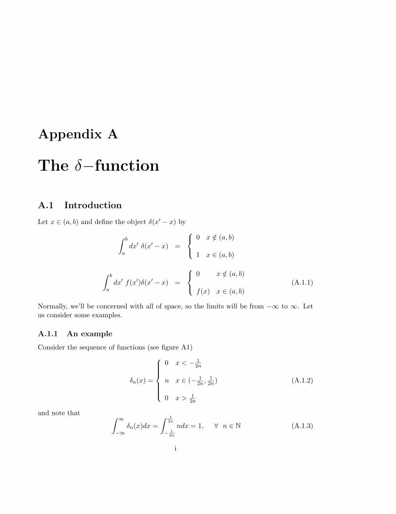
Appendix A
The δ−function
A.1 Introduction
Let x ∈ (a, b) and define the object δ(x′ − x) by
∫ b
adx′ δ(x′ − x) =
0 x /∈ (a, b)
1 x ∈ (a, b)
∫ b
adx′ f(x′)δ(x′ − x) =
0 x /∈ (a, b)
f(x) x ∈ (a, b)(A.1.1)
Normally, we’ll be concerned with all of space, so the limits will be from −∞ to ∞. Letus consider some examples.
A.1.1 An example
Consider the sequence of functions (see figure A1)
δn(x) =
0 x < − 1
2n
n x ∈ (− 12n ,
12n)
0 x > 12n
(A.1.2)
and note that ∫ ∞−∞
δn(x)dx =
∫ 12n
− 12n
ndx = 1, ∀ n ∈ N (A.1.3)
i
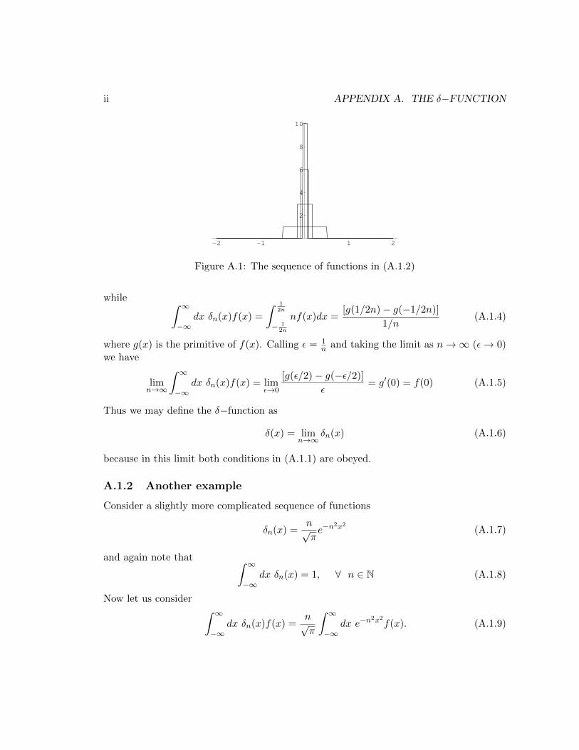
ii APPENDIX A. THE δ−FUNCTION
-2 -1 1 2
2
4
6
8
10
Figure A.1: The sequence of functions in (A.1.2)
while ∫ ∞−∞
dx δn(x)f(x) =
∫ 12n
− 12n
nf(x)dx =[g(1/2n)− g(−1/2n)]
1/n(A.1.4)
where g(x) is the primitive of f(x). Calling ε = 1n and taking the limit as n→∞ (ε→ 0)
we have
limn→∞
∫ ∞−∞
dx δn(x)f(x) = limε→0
[g(ε/2)− g(−ε/2)]
ε= g′(0) = f(0) (A.1.5)
Thus we may define the δ−function as
δ(x) = limn→∞
δn(x) (A.1.6)
because in this limit both conditions in (A.1.1) are obeyed.
A.1.2 Another example
Consider a slightly more complicated sequence of functions
δn(x) =n√πe−n
2x2 (A.1.7)
and again note that ∫ ∞−∞
dx δn(x) = 1, ∀ n ∈ N (A.1.8)
Now let us consider ∫ ∞−∞
dx δn(x)f(x) =n√π
∫ ∞−∞
dx e−n2x2f(x). (A.1.9)
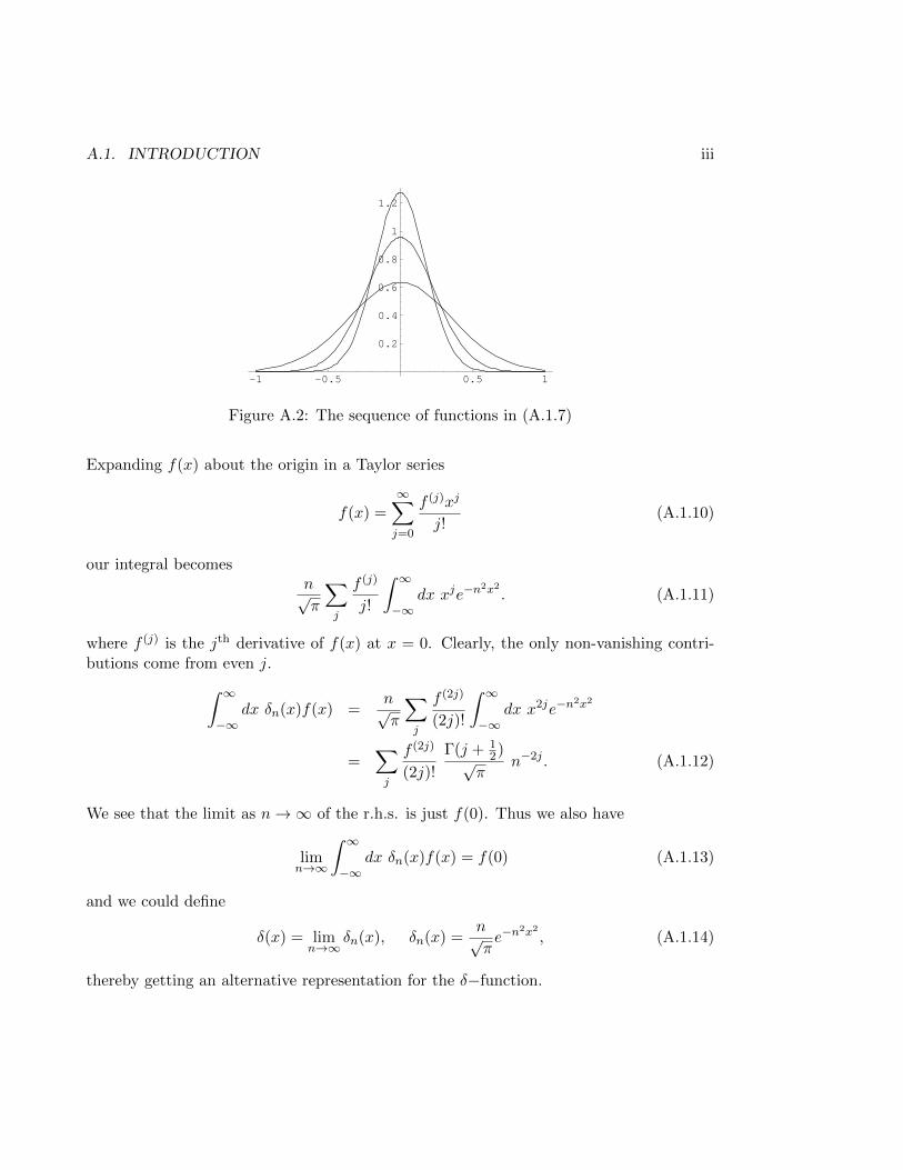
A.1. INTRODUCTION iii
-1 -0.5 0.5 1
0.2
0.4
0.6
0.8
1
1.2
Figure A.2: The sequence of functions in (A.1.7)
Expanding f(x) about the origin in a Taylor series
f(x) =∞∑j=0
f (j)xj
j!(A.1.10)
our integral becomesn√π
∑j
f (j)
j!
∫ ∞−∞
dx xje−n2x2 . (A.1.11)
where f (j) is the jth derivative of f(x) at x = 0. Clearly, the only non-vanishing contri-butions come from even j.∫ ∞
−∞dx δn(x)f(x) =
n√π
∑j
f (2j)
(2j)!
∫ ∞−∞
dx x2je−n2x2
=∑j
f (2j)
(2j)!
Γ(j + 12)
√π
n−2j . (A.1.12)
We see that the limit as n→∞ of the r.h.s. is just f(0). Thus we also have
limn→∞
∫ ∞−∞
dx δn(x)f(x) = f(0) (A.1.13)
and we could define
δ(x) = limn→∞
δn(x), δn(x) =n√πe−n
2x2 , (A.1.14)
thereby getting an alternative representation for the δ−function.
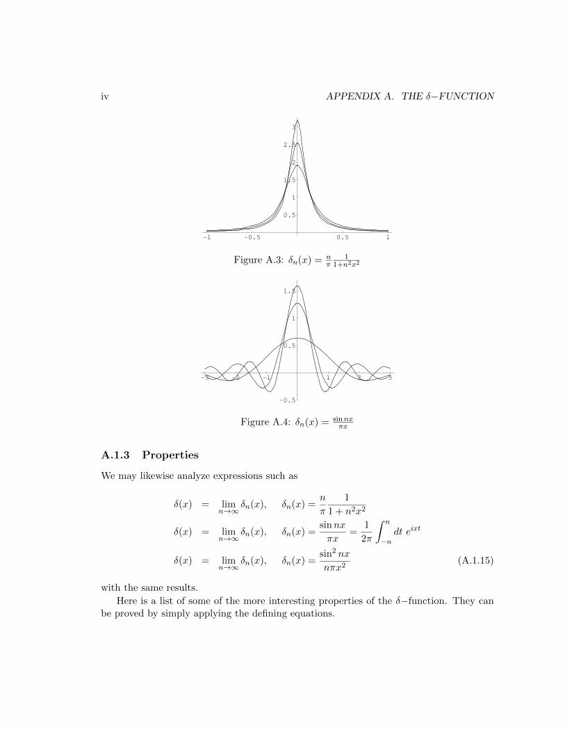
iv APPENDIX A. THE δ−FUNCTION
-1 -0.5 0.5 1
0.5
1
1.5
2
2.5
3
Figure A.3: δn(x) = nπ
11+n2x2
-3 -2 -1 1 2 3
-0.5
0.5
1
1.5
Figure A.4: δn(x) = sinnxπx
A.1.3 Properties
We may likewise analyze expressions such as
δ(x) = limn→∞
δn(x), δn(x) =n
π
1
1 + n2x2
δ(x) = limn→∞
δn(x), δn(x) =sinnx
πx=
1
2π
∫ n
−ndt eixt
δ(x) = limn→∞
δn(x), δn(x) =sin2 nx
nπx2(A.1.15)
with the same results.
Here is a list of some of the more interesting properties of the δ−function. They canbe proved by simply applying the defining equations.
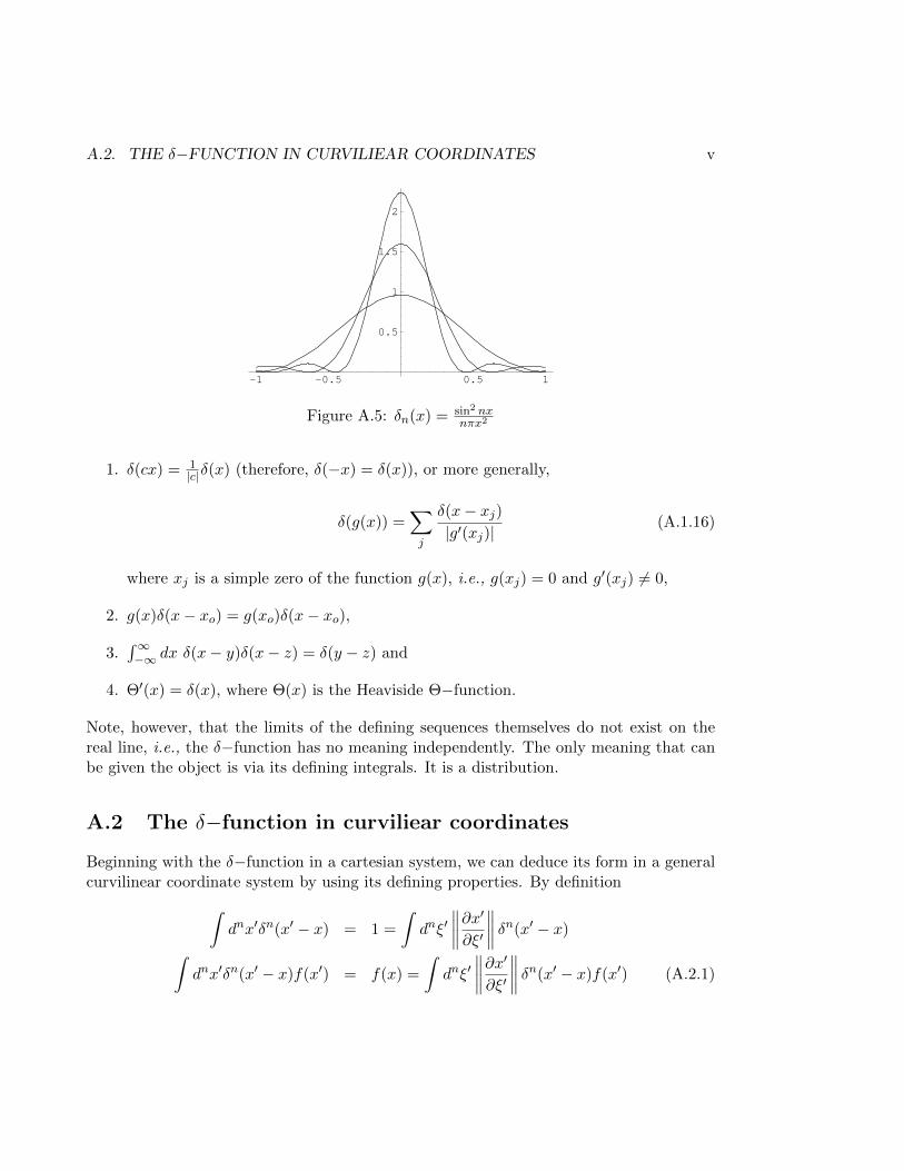
A.2. THE δ−FUNCTION IN CURVILIEAR COORDINATES v
-1 -0.5 0.5 1
0.5
1
1.5
2
Figure A.5: δn(x) = sin2 nxnπx2
1. δ(cx) = 1|c|δ(x) (therefore, δ(−x) = δ(x)), or more generally,
δ(g(x)) =∑j
δ(x− xj)|g′(xj)|
(A.1.16)
where xj is a simple zero of the function g(x), i.e., g(xj) = 0 and g′(xj) 6= 0,
2. g(x)δ(x− xo) = g(xo)δ(x− xo),
3.∫∞−∞ dx δ(x− y)δ(x− z) = δ(y − z) and
4. Θ′(x) = δ(x), where Θ(x) is the Heaviside Θ−function.
Note, however, that the limits of the defining sequences themselves do not exist on thereal line, i.e., the δ−function has no meaning independently. The only meaning that canbe given the object is via its defining integrals. It is a distribution.
A.2 The δ−function in curviliear coordinates
Beginning with the δ−function in a cartesian system, we can deduce its form in a generalcurvilinear coordinate system by using its defining properties. By definition∫
dnx′δn(x′ − x) = 1 =
∫dnξ′
∥∥∥∥∂x′∂ξ′
∥∥∥∥ δn(x′ − x)∫dnx′δn(x′ − x)f(x′) = f(x) =
∫dnξ′
∥∥∥∥∂x′∂ξ′
∥∥∥∥ δn(x′ − x)f(x′) (A.2.1)
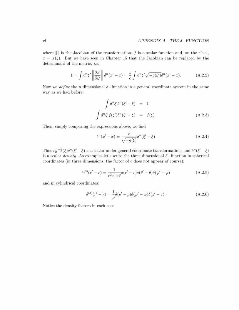
vi APPENDIX A. THE δ−FUNCTION
where ‖‖ is the Jacobian of the transformation, f is a scalar function and, on the r.h.s.,x = x(ξ). But we have seen in Chapter 15 that the Jacobian can be replaced by thedeterminant of the metric, i.e.,
1 =
∫dnξ′
∥∥∥∥∂x′∂ξ′
∥∥∥∥ δn(x′ − x) =1
c
∫dnξ′
√−g(ξ′)δn(x′ − x). (A.2.2)
Now we define the n dimensional δ−function in a general coordinate system in the sameway as we had before: ∫
dnξ′δn(ξ′ − ξ) = 1∫dnξ′f(ξ′)δn(ξ′ − ξ) = f(ξ). (A.2.3)
Then, simply comparing the expressions above, we find
δn(x′ − x) =c√−g(ξ)
δn(ξ′ − ξ) (A.2.4)
Thus cg−12 (ξ)δn(ξ′− ξ) is a scalar under general coordinate transformations and δn(ξ′− ξ)
is a scalar density. As examples let’s write the three dimensional δ−function in sphericalcoordinates (in three dimensions, the factor of c does not appear of course):
δ(3)(~r′ − ~r) =1
r2 sin θδ(r′ − r)δ(θ′ − θ)δ(ϕ′ − ϕ) (A.2.5)
and in cylindrical coordinates:
δ(3)(~r′ − ~r) =1
ρδ(ρ′ − ρ)δ(ϕ′ − ϕ)δ(z′ − z). (A.2.6)
Notice the density factors in each case.


![[Kibble] - Classical Mechanics](https://static.fdocuments.us/doc/165x107/552056344a79596f718b4715/kibble-classical-mechanics.jpg)