Classical Electrodynamics (2 hrs) and Special Relativity...
120
Classical Electrodynamics (2 hrs) and Special Relativity (1 hr) CERN Accelerator School, 8-21 September 2019, Vysoke-Tatry, Slovakia
Transcript of Classical Electrodynamics (2 hrs) and Special Relativity...

Classical Electrodynamics (2 hrs) and Special Relativity (1 hr)
CERN Accelerator School, 8-21 September 2019, Vysoke-Tatry, Slovakia

Recommended Reading Material (in this order)
[1 ] R.P. Feynman, Feynman lectures on Physics, Vol2.
[2 ] Proceedings of CAS: RF for accelerators,
Ebeltoft, Denmark, 8-17 June 2010, Edited by R. Bailey, CERN-2011-007.
[3 ] J.D. Jackson, Classical Electrodynamics (Wiley, 1998 ..)
[4 ] L. Landau, E. Lifschitz, The Classical Theory of F ields, Vol2.
(Butterworth-Heinemann, 1975)
[5 ] J. Slater, N. Frank, Electromagnetism, (McGraw-Hill, 1947, and Dover
Books, 1970)

OUTLINE - following this strategy
This does not replace a full course (i.e. ≈ 60 hours, some additional
material in backup slides, details in bibliography)
Also, it cannot be treated systematically without special relativity.
The main topics discussed:
Basic electromagnetic phenomena, to arrive at:
Maxwell’s equations
Lorentz force, charged particles in electromagnetic fields
Electromagnetic waves in vacuum
Electromagnetic waves in conducting media, waves in RF cavities
and wave guides
Special Relativity should come in here to sort out some issues

Variables, notations and units used in this lecture
Formulae use SI units throughout.
~E(~r, t) = electric field [V/m]~H(~r, t) = magnetic field [A/m]~D(~r, t) = electric displacement [C/m2]~B(~r, t) = magnetic flux density [T]
q = electric charge [C]
ρ(~r, t) = electric charge density [C/m3]~I, ~j(~r, t) = current [A], current density [A/m2]
µ0 = permeability of vacuum, 4 π · 10−7 [H/m or N/A2]
ǫ0 = permittivity of vacuum, 8.854 ·10−12 [F/m]
c = speed of light in free space, 299792458.0 [m/s]
h = Planck constant, 6.62607 ·10−34 [J s]

FAQ: do we really need Maxwell’s equations (instead of explaining the phenomena) ?
- They are fairly abstract and use some advanced mathematics, but they do not
really say what is happening to fields and particles
- However they provide a (very successful) framework to model the observations,
but cannot really call it a ”theory”).
- Some early attempts tried to explain fields as some kind of ”gear wheels” or
some ”stress” between some kind of material (would still be compatible with
Maxwell)
What is needed is a set of concepts to conveniently ”describe” the effects in
mathematical terms to arrive at:
A formulation, to figure out the characteristics of a solution of a problem,
without actually solving it.
Maxwell’s equations do exactly that job !

- ELECTROSTATICS -
Electrostatics deals with:
- Charges Q
- (Static) Electric fields ~E generated by the charges

Recap: vectors and vector calculus define a special vector ∇
called the ”gradient”: ∇ def= (
∂
∂x,
∂
∂y,
∂
∂z)
Can be used like any other vector (e.g. in vector and scalar products),
for example on a vector ~F (x, y, z) or a scalar function φ(x, y, z):
∇ · ~F =∂
∂xF1 +
∂
∂yF2 +
∂
∂zF3 =
∂F1
∂x+
∂F2
∂y+
∂F3
∂z
∇× ~F =
(∂F3
∂y− ∂F2
∂z,
∂F1
∂z− ∂F3
∂x,
∂F2
∂x− ∂F1
∂y
)
∇φ = (∂φ
∂x,
∂φ
∂y,
∂φ
∂z)
A very versatile object ...

Consider it an operator-in-waiting (for something to work on ..)
Depending how it is used in products the results are very different:
∇ · ~F is a scalar ( e.g. ”density” of a source, see later)
∇ φ is a ”honest” vector ( e.g. electric field ~E, force )
∇× ~F is a pseudo-vector
Works also on matrices (of course) and on itself (e.g.):
∇ · ∇ (also written as ∆)
∇× (∇× ~F ) = ∇ · (∇ · ~F ) − ∆~F
etc. all kind of contraptions ...

Two operations with ∇ acting on vectors have special names:
DIVERGENCE (scalar product of ∇ with a vector):
div(~F )def= ∇ · ~F =
∂F1
∂x+
∂F2
∂y+
∂F3
∂z
Physical significance: measure of something ”coming out”
CURL (vector product of ∇ with a vector):
curl(~F )def= ∇× ~F =
(
∂F3
∂y− ∂F2
∂z,
∂F1
∂z− ∂F3
∂x,
∂F2
∂x− ∂F1
∂y
)
Physical significance: measure of something ”circulating”
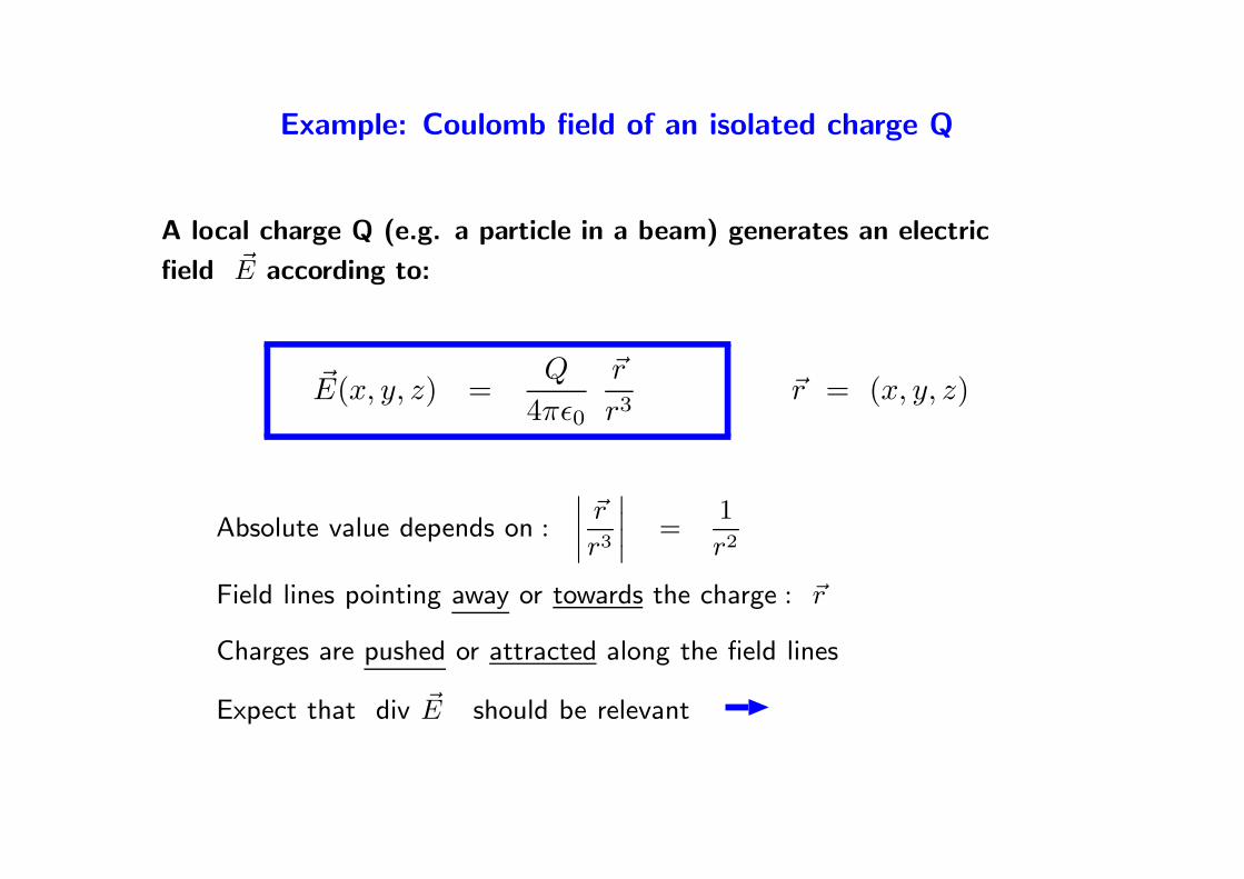
Example: Coulomb field of an isolated charge Q
A local charge Q (e.g. a particle in a beam) generates an electric
field ~E according to:
~E(x, y, z) =Q
4πǫ0
~r
r3~r = (x, y, z)
Absolute value depends on :
∣∣∣∣
~r
r3
∣∣∣∣
=1
r2
Field lines pointing away or towards the charge : ~r
Charges are pushed or attracted along the field lines
Expect that div ~E should be relevant

We can do the (non-trivial∗) computation of the divergence:
div ~E = ∇ ~E =dEx
dx+
dEy
dy+
dEz
dz=
ρ
ǫ0
(negative charges) (positive charges)
∇ · ~E < 0 ∇ · ~E > 0
Divergence related to charge density ρ∗∗ generating the field ~E
Charge density ρ is charge per volume∗∗∗: ρ =Q
V=⇒
∫∫∫
ρ dV = Q
∗ see later∗∗ sometime called ”source density”∗∗∗ becomes important later

Counting charges and field lines (a simple pictorial form)
Surface integrals: integrate (adding up) field vectors passing through a surface S
(or area A), we obtain the Flux
Φ =N∑
i
~E =Q
ǫ0
Intuitively: count ”arrows”, how many (N) and how long Qi (strong fields)
The surface can also be wrapped up (closed) to encompass a volume, e.g.:

Replace individual charges by charge density:
qi =⇒ ρ(x, y, z) i.e. charge per unit volume dV
For a charge density the sum is replaced by an integral of ~E through the surface
element d ~A:
Φ =N∑
i
~E
∫
S
~E d ~A
and
∫
V
ρ dV = Q
The volume V is the one enclosed by the surface S
This holds for any arbitrary (closed) surface S, and:
Does not matter how the particles are distributed inside the volume
Does not matter whether the particles are moving (for this part)
Does not matter whether the particles are in vacuum or material

Using this vector calculus (here you have to believe me) :
∫
S
~E · d ~A =
∫
V
∇ ~E · dV
︸ ︷︷ ︸
Gauss′ formula
(relates surface and volume integrals)
∇ ~E =ρ
ǫ0written as divergence : div ~E
ΦE =∫
S
~E · d ~A =∫
V
ρ
ǫ0· dV =
Q
ǫ0= ΦE
Flux of electric field ~E through any closed surface is proportional to net electric
charge Q enclosed in the region (Gauss’ Theorem).
Written with charge density ρ we have:
div ~E = ∇ · ~E =∂Ex
∂x+
∂Ey
∂y+
∂Ez
∂z=
ρ
ǫ0

Simplest possible example: flux from a charge q
+q
dAE
A charge q generates a field ~E according to (Coulomb):
~E =q
4πǫ0
~r
r3
Enclose it by a sphere: ~E = const. on a sphere (area is 4π · r2):∫
sphere
~E · d ~A =q
4πǫ0
∫
sphere
dA
r2=
q
ǫ0
Surface integral through sphere A is charge inside the sphere (any radius, any shape)
Exercise: compute the surface integral for the cube, the result will be interesting

Once more to remember: Gauss’ theorem to evaluate flux integral:
dA
F
enclosed volume (V)
closed surface (A)
∫∫
A
~E · d ~A =∫∫∫
V
∇ · ~E · dV or
∫∫
A
~E · d ~A =∫∫∫
V
div ~E · dV
Integral through closed surface
(flux) is integral of divergence
in the enclosed volume
Surface integral related to the divergence from the enclosed volume
Sum (integral) of all sources inside the volume gives the flux out of this
region

Arrive at: Maxwell’s first equation using Gauss’s
density ρ and charge Q :
∫
V
ρ
ǫ0· dV =
Q
ǫ0
∫
A
~E · d ~A =
∫
V
∇ · ~E · dV
︸ ︷︷ ︸
Gauss theorem
=Q
ǫ0=
∫
V
ρ
ǫ0· dV
Written with charge density ρ we get Maxwell’s first equation:
Maxwell (I): div ~E = ∇ · ~E =ρ
ǫ0
The higher the charge density: The larger the divergence of the field
Some calculations of DIV and CURL: simplest possible charge distribution - point
charge
~E =q
4πǫ0· ~r
r3
What are div ~E and curl ~E for a point charge ?
First step: compute all derivatives (used for DIV and CURL)
∂E(x,y,z)
∂(x,y,z)

∂Ex
∂x=
Q
4πǫ0
(
1
R3− 3x2
R5
)
∂Ex
∂y=
−3Q
4πǫ0
xy
R5
∂Ex
∂z=
−3Q
4πǫ0
xz
R5
∂Ey
∂x=
−3Q
4πǫ0
xy
R5
∂Ey
∂y=
Q
4πǫ0
(
1
R3− 3y2
R5
)
∂Ey
∂z=
−3Q
4πǫ0
yz
R5
∂Ez
∂x=
−3Q
4πǫ0
xz
R5
∂Ez
∂y=
−3Q
4πǫ0
yz
R5
∂Ez
∂z=
Q
4πǫ0
(
1
R3− 3z2
R5
)

∂Ex
∂x=
Q
4πǫ0
(
1
R3− 3x2
R5
)
∂Ex
∂y=
−3Q
4πǫ0
xy
R5
∂Ex
∂z=
−3Q
4πǫ0
xz
R5
∂Ey
∂x=
−3Q
4πǫ0
xy
R5
∂Ey
∂y=
Q
4πǫ0
(
1
R3− 3y2
R5
)
∂Ey
∂z=
−3Q
4πǫ0
yz
R5
∂Ez
∂x=
−3Q
4πǫ0
xz
R5
∂Ez
∂y=
−3Q
4πǫ0
yz
R5
∂Ez
∂z=
Q
4πǫ0
(
1
R3− 3z2
R5
)
div ~E =∂Ex
∂x+
∂Ey
∂y+
∂Ez
∂z=
Q
4πǫ0
(
3
R3− 3
R5(x2 + y2 + z2)
)

∂Ex
∂x=
Q
4πǫ0
(
1
R3− 3x2
R5
)
∂Ex
∂y=
−3Q
4πǫ0
xy
R5
∂Ex
∂z=
−3Q
4πǫ0
xz
R5
∂Ey
∂x=
−3Q
4πǫ0
xy
R5
∂Ey
∂y=
Q
4πǫ0
(
1
R3− 3y2
R5
)
∂Ey
∂z=
−3Q
4πǫ0
yz
R5
∂Ez
∂x=
−3Q
4πǫ0
xz
R5
∂Ez
∂y=
−3Q
4πǫ0
yz
R5
∂Ez
∂z=
Q
4πǫ0
(
1
R3− 3z2
R5
)
curl ~E = (∂Ez
∂y− ∂Ey
∂z,
∂Ex
∂z− ∂Ez
∂x,
∂Ey
∂x− ∂Ex
∂z) = (0, 0, 0)
(there is nothing circulating around a point charge)

In general: Because there is nothing circulating (curl ~E = 0) one can
derive the field ~E from a scalar electrostatic potential φ(x, y, z), i.e.:
~E = − grad φ = −∇φ = − (∂φ
∂x,∂φ
∂y,∂φ
∂z)
then we have
∇ ~E = −∇2φ = − (∂2φ
∂x2+
∂2φ
∂y2+
∂2φ
∂z2) =
ρ(x, y, z)
ǫ0
This is called Poisson’s equation
All we need is φ to get the fields Example

A very important example: 3D Gaussian distribution
ρ(x, y, z) =Q
σxσyσz
√2π
3 exp
(
− x2
2σ2x
− y2
2σ2y
− z2
2σ2z
)
(σx, σy, σz r.m.s. sizes)
φ(x, y, z, σx, σy, σz) =Q
4πǫ0
∫
∞
0
exp(− x2
2σ2x+t
− y2
2σ2y+t
− z2
2σ2z+t
)√
(2σ2x + t)(2σ2
y + t)(2σ2z + t)
dt
For a derivation, see e.g. W. Herr, Beam-Beam Effects,
in Proceedings CAS Zeuthen, 2003, CERN-2006-002, and references therein.

This gives the compact formulae for the fields:
Ex =ne
2ǫ0√
2π(σ2x − σ2
y)Im
erf
x + iy√
2(σ2x − σ2
y)
− e
(
−x2
2σ2x
+y2
2σ2y
)
erf
xσyσx
+ iy σxσy
√
2(σ2x − σ2
y)
Ey =ne
2ǫ0√
2π(σ2x − σ2
y)Re
erf
x + iy√
2(σ2x − σ2
y)
− e
(
−x2
2σ2x
+y2
2σ2y
)
erf
xσyσx
+ iy σxσy
√
2(σ2x − σ2
y)
wherer erf is the complex error function
These formulae are often used to evaluate the forces due to beam-beam effects

Very important in practice:
Poisson’s equation in Polar coordinates, i.e. 2D (r, ϕ)
1
r
∂
∂r
(
r∂φ
∂r
)
+1
r2∂2φ
∂ϕ2= − ρ
ǫ0
Poisson’s equation in Cylindrical coordinates (r, ϕ, z)
1
r
∂
∂r
(
r∂φ
∂r
)
+1
r2∂2φ
∂ϕ2+
∂2φ
∂z2= − ρ
ǫ0
Poisson’s equation in Spherical coordinates (r, θ, ϕ)
1
r2∂
∂r
(
r2∂φ
∂r
)
+1
r2 sin θ
∂
∂θ
(
sin θ∂φ
∂θ
)
+1
r2 sin θ
∂2φ
∂ϕ2= − ρ
ǫ0

Spherical coordinates sound like a good choice for local charges, e.g. point charges
What are div and curl ??
div ~E(r, θ, ϕ) =1
r2∂
∂r(r2Er) +
1
r sin θ
∂
∂θ(sin θEθ) +
1
r sin θ
∂Eϕ
∂ϕ
(very useful !)
curl ~E(r, θ, ϕ) =er
r sin θ
(∂(Eϕ sin θ)
∂θ− ∂Eθ
∂ϕ
)
+
eθr
(1
sin θ
∂Er
∂ϕ− Eϕ
∂r(rEϕ
)
+eϕr
(∂(rEθ)
∂r− ∂Er
∂θ
)
Note: eθ, er, eϕ are the corresponding orthogonal unit vectors
(useful, but no so much used !)

Try it on a point charge
~E = −∇Ψ(r) =Q
4πǫ0· ~r
r3
div ~E(r, θ, ϕ) =1
r2∂
∂r(r2Er) +
1
r sin θ
∂
∂θ(sin θEθ)
︸ ︷︷ ︸
≡ 0
+1
r sin θ
∂Eϕ
∂ϕ︸ ︷︷ ︸
≡ 0
Only the radial component is non-zero:
then : div ~E(r, θ, ϕ) =1
r2∂
∂r(r2Er)
div ~E(r, θ, ϕ) =1
r2∂
∂r
(r2 ·Q4πǫ0r2
)
=1
r2∂
∂r
(Q
4πǫ0
)
= ???
(non-trivial indeed ...)

What about magnetic fields ? ...
They have the direction (by definition): magnetic field lines from
North to South
Field lines of ~B are always closed
Magnets (e.g. compass) are pushed or attracted along the field lines
What about divergence of magnetic fields ?

Enclose it again by a surface - the result is found immediately:
∫ ∫
A
~B d ~A =
∫ ∫ ∫
V
∇ ~B dV = 0
Volume (thus dV) is never = 0
∇ ~B = div ~B = 0
What goes into the closed surface also goes out
Maxwell’s second equation: ∇ ~B = div ~B = 0
Physical significance: (probably) no Magnetic Monopoles

Enter Faraday: allow changing flux through an area
static flux : Ω =
∫
A
~B · d ~A changing flux :∂Ω
∂t=
∫
A
∂( ~B)
∂t· d ~A
NS
staticNS
v
I
I
NS
v
I
I
Moving the magnet changes the flux: more or fewer passing through the
area (use a conducting coil, e.g. wedding ring) =⇒
Induces a circulating (curling) electric field ~E in the coil which ”pushes”
charges around the coil =⇒
Moving charges: Current I in the coil (observe its direction ..)

Experimental evidence:
It does not matter whether the magnet or the coil is moved (same
direction of induced current):
NS
v
I
I
NS
v

Experimental evidence:
It does not matter whether the magnet or the coil is moved (same
direction of induced current):
NS
v
I
I
NS
v
If you think it is obvious - no :
This was the reason for Einstein to develope special relativity !!!
Again: Maxwell different in the two systems (see lecture on Relativity)

Formally: A changing flux Ω through an area A produces circular electric
field ~E, ”pushing” charges =⇒ a current I
−∂Ω
∂t=
∂
∂t
flux Ω︷ ︸︸ ︷∫
A
~B · d ~A =
∮
C
~E · d~r
︸ ︷︷ ︸
pushed charges
Flux can be changed by:
- Change of magnetic field ~B with time t (e.g. transformers)
- Change of area A with time t (e.g. dynamos)
How to count ”pushed charges”
∫
C
~E · d~r is a line integral

Line integrals sum up ”pushes” along lines or curves:
Edr
1
2
”lines” can be open or closed
Sum along all line elements d~r
2∫
1
~E · d~r or∫
C
~E · d~r
E dr
C

Everyday example ..
Line integrals: sum up ”pushes” along the two Lines/Routes
Optimize: e.g. fuel consumption, time of flight (saves 1 hour !)
Like surface integral, the closed line integral∫
C
~E · d~r can be re-written:

Used in the following: Stoke’s theorem
-6
-4
-2
0
2
4
6
-6 -4 -2 0 2 4 6
y
x
Line Integral of a vector field ∮
C
~E · d~r =∫∫
A
∇× ~E · d ~A or
∮
C
~E · d~r =∫∫
A
curl ~E · d ~A
obviously : div ~E = 0
Summing up all vectors inside the area: net effect is the sum along the
closed curve
measures something that is circulating (”curling”) inside and how
strongly

Use this theorem for a coil enclosing a closed area
∫
A
− ∂ ~B
∂td ~A =
∫
A
∇× ~E d ~A =
∮
C
~E · d~r︸ ︷︷ ︸
Stoke′s formula
∫
A
− ∂ ~B
∂td ~A =
∫
A
∇× ~E d ~A
︸ ︷︷ ︸
same Integration
Re-written: changing magnetic field through an area induces circulating
electric field around the area (Faraday)
Maxwell’ 3rd equation −∂ ~B
∂t= ∇× ~E = curl ~E

Next: Maxwell’s fourth equation (part 1) ...
From Ampere’s law, for example current density ~j:∫
A
∇× ~B d ~A =
∮
C
~B · d~r =
∫
A
µ0~j d ~A
~j : ”amount” of charges through area ~A∫
A
µ0~j d ~A = µ0 I (total current)
Static electric current induces circular magnetic field (e.g. in magnets)
Using the same argument as before (the same integral formula):
∇× ~B = µ0~j

An important application:
For a static electric current I in a single (infinitely long) wire we get
Biot-Savart law (using the area of a circle A = r2 · π, we can easily do
the integral):
induced magneticfield
current
~B =µ0
4π
∮
~j · ~r · d~rr3
~B =µ0
2π
~j
r
Application: magnetic field calculations in wires

Maxwell’s fourth equation (part 2) ...
Charging capacitor: Current enters left plate - leaves from right plate,
builds up an electric field between plates produces a ”current”
during the charging process
E
jd jd
+Q −Q
+
+
++
+
++
+
−
−
− −
−
− −
−
0
1
2
3
4
5
0 2 4 6 8 10
char
ging
cur
rent
a.u
.
char
ge o
n ca
paci
tor
time
Charging Capacitor
current
charge
Q(t) = C · Vb · (1 − exp(−t/RC)) and I(t) =Vb
Rexp(−t/RC)

Part 2: Maxwell’s fourth equation
Charging capacitor: Current enters left plate - leaves from right plate,
builds up an electric field between plates produces a ”current”
during the charging process
jd jd
E
+Q −Q
+
+
++
+
++
+
−
−
− −
−
− −
−
Displacement Current :
~jd =d ~E
dt
This is not a current from charges moving through a wire
This is a ”current” from time varying electric fields
Once charged: fields are constant, (displacement) ”current” stops

Cannot distinguish the origin of a current - apply Ampere’s law to jd
Displacement current jd produces magnetic field, just like
”real currents” do ...
jd jd
E B
+Q −Q
+
+
++
+
++
+
−
−
− −
−
− −
−
Time varying electric field induces time varying circular magnetic
field (using the current density ~jd)
∇× ~B = µ0~jd = ǫ0µ0
d ~E
dt

Bottom line:
Magnetic fields ~B can be generated by two different ”currents”:
∇× ~B = µ0~j (electrical current)
∇× ~B = µ0~jd = ǫ0µ0
∂ ~E
∂t(displacement current)
or putting them together to get Maxwell’s fourth equation:
∇× ~B = µ0(~j + ~jd) = µ0~j + ǫ0µ0
∂ ~E
∂t
or in integral form:
∫
A
∇× ~B · d ~A =
∫
A
(
µ0~j + ǫ0µ0
∂ ~E
∂t
)
· d ~A

Summary: Maxwell’s Equations
∫
A
~E · d ~A =Q
ǫ0∫
A
~B · d ~A = 0
∮
C
~E · d~r = −∫
A
(
d ~B
dt
)
· d ~A
∮
C
~B · d~r =
∫
A
(
µ0~j + µ0ǫ0
d ~E
dt
)
· d ~A
Written in Integral form

Summary: Maxwell’s Equations
∇ ~E =ρ
ǫ0
∇ ~B = 0
∇× ~E = −d ~B
dt
∇× ~B = µ0~j + µ0ǫ0
d ~E
dt
Written in Differential form (my preference)

V.G.F.A.Q:
Why : Why Not :
div ~E =ρ
ǫ0
∫
A
~E · d ~A =Q
ǫ0
curl ~E = −d ~B
dt
∮
C
~E · d~r = −∫
A
(
d ~B
dt
)
· d ~A
div ~B = 0
∫
A
~B · d ~A = 0
curl ~B = µ0~j + µ0ǫ0
d ~E
dt
∮
C
~B · d~r =
∫
A
(
µ0~j + µ0ǫ0
d ~E
dt
)
· d ~A

div ~E =ρ
ǫ0something ( ~E) flowing out
∫
A
~E · d ~A =Q
ǫ0???
curl ~E = −d ~B
dtsomething ( ~E) circulating
∮
C
~E · d~r = −∫
A
(
d ~B
dt
)
· d ~A ???

Maxwell’s Equations - compact
1. Electric fields ~E are generated by charges and proportional
to total charge
2. Magnetic monopoles do (probably) not exist
3. Changing magnetic flux generates circular electric
fields/currents
4.1 Changing electric flux generates circular magnetic fields
4.2 Static electric current generates circular magnetic fields

Changing fields: Powering and self-induction
- If the current is not static:
- Primary magnetic flux ~B changes with changing current
Induces an electric field, resulting in a current and induced
magnetic field ~Bi
Induced current will oppose a change of the primary current
If we want to change a current to ramp a magnet ...

Ramp rate defines required Voltage:
U = −L∂I
∂t
Inductance L in Henry (H)
Example:
- Required ramp rate: 10 A/s
- With L = 15.1 H per powering sector
Required Voltage is ≈ 150 V

Surprise - as is always the case:
Units: Gauss law Ampere/Maxwell
SI ∇ ~E =ρ
ǫ0∇× ~B = µ0
~j + µ0ǫ0d ~E
dt
Electro-static (ǫ0 = 1) ∇ ~E = 4πρ ∇× ~B =4π
c2~j +
1
c2d ~E
dt
Electro-magnetic (µ0 = 1) ∇ ~E = 4πc2ρ ∇× ~B = 4π~j +1
c2d ~E
dt
Gauss cgs ∇ ~E = 4πρ ∇× ~B =4π
c~j +
1
c
d ~E
dt
Lorentz ∇ ~E = ρ ∇× ~B =1
c~j +
1
c
d ~E
dt
Also: ~BGauss =
√4π
µ0
~BSI ρGauss =ρSI
√4πǫ0
and so on .....

That’s not all Electromagnetic fields in material
In vacuum:~D = ǫ0 · ~E, ~B = µ0 · ~H
In a material:~D = ǫr · ǫ0 · ~E = ǫ0 ~E + ~P
~B = µr · µ0 · ~H = µ0~H + ~M
Origin: ~Polarization and ~Magnetization
ǫr( ~E,~r, ω) ǫr is relative permittivity ≈ [1− 105]
µr( ~H,~r, ω) µr is relative permeability ≈ [0(!)− 106]
(i.e.: linear, isotropic, non-dispersive)

Polarization ~P : displacement of charges in non-conducting material
−−−−−−−−
++++++
+++
+
−
E
Appears as electric dipole
~P = ξe · ~E (ξe is electric susceptibility)
Dielectric displacement follows: ~D = (1 + 4πξe) ~E = ǫ · ~E

Magnetism: occurence of circular currents of atomic electrons
Classification of magnetic material properties:
Diamagnetism repelled µ < 1 ξm < 0 typical: ξm ≈ − 10−7
Paramagnetism aligned µ > 1 ξm > 0 typical: ξm ≈ + 10−7
Ferromagnetism aligned µ ≫ 1 ξm ≫ 0 typical: ξm ≈ + 106
Diamagnetism: Atoms and molecules without magnetic moment
Paramagnetism: Atoms and molecules with magnetic moment
Ferromagnetism: Saturation magnetization occur within microscopic
domains (Weiss domains)

Magnetism in ferromagnetic: not rigorous - just to get an idea ...
no field weak field strong field
domain walls
Unmagnetized Iron: spontaneous magnetization around seeds, leading to
”Weiss domains”
Randomly oriented domains cancel out
With external fields: domain walls move - domains in direction of external
field ”grow”! They do not align (although this is sometimes said)!
Magnetic field follows : ~B = (1 + 4πξm) ~H = µ · ~H
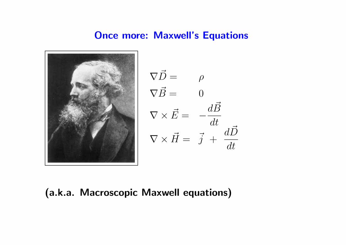
Once more: Maxwell’s Equations
∇ ~D = ρ
∇ ~B = 0
∇× ~E = −d ~B
dt
∇× ~H = ~j +d ~D
dt
(a.k.a. Macroscopic Maxwell equations)

Something on potentials (needed in lecture on Relativity):
In general: Scalar Potentials are related to static field conditions, Vector Potentials are
related to dynamic field conditions
Electric fields can be derived from a (scalar) potential φ:
~E = − ~∇ · φ
Magnetic fields can be derived from a (vector) potential ~A:
~B = ~∇ × ~A = curl ~A
Combining Maxwell(I) + Maxwell(III):
~E = − ~∇ · φ −∂ ~A
∂t
Fields can be written as derivatives of scalar and vector potentials Φ(x, y, z) and ~A(x, y, z)
But watch out and remember for later: ~∇ · ... versus ~∇ × ... !
(absolute values of potentials Φ and ~A can not be measured ..)

The Coulomb potential of a static charge q is written as:
Ψ(~r) =1
4πǫ0· q
|~r − ~rq|
[
or
∫1
4πǫ0· ρ(~rq)
|~r − ~rq|
]
where ~r is the observation point∗ and ~rq the location of the charge
The vector potential is linked to the current ~j:
∇2 ~A = µ0~j
The knowledge of the potentials allows the computation of the
fields see lecture on relativity (fields of moving charges)
∗ a shameless lie: one cannot observe/measure a potential (only fields) !

Accelerator magnets Multipole expansion
If Ψ is periodic∗) in θ, the components in cylindrical coordinates are:
Br(θ, r) = −(
∂Ψ
∂r
)
=∞∑
n=1
C(n)
(
r
Rref
)n−1
sin(n(θ − αn)) and
Bθ(θ, r) = −(
1
r
)(
∂Ψ
∂θ
)
=∞∑
n=1
C(n)
(
r
Rref
)n−1
cos(n(θ − αn))
C(n) is the strength of the 2n-pole component of the total field
Rref is a reference radius (LHC: 17 mm for 28 mm aperture, typical ratio)
αn is a constant (related to the orientation of the 2n component)
∗) a good assumption for accelerator magnets

The n-th component in Br(r, θ) has n South poles and n North poles
as a function of the azimuthal angle θ
This implies (for any n):
θS =π
2n+ αn;
5π
2n+ αn;
9π
2n+ αn; ... (South poles)
θN =3π
2n+ αn;
7π
2n+ αn;
11π
2n+ αn; ... (North poles)
A focusing Quadrupole (n = 2, α2 = 0):
θS = 45deg; 225 deg; 405 deg; ..... (South poles)
θN = 135deg; 315 deg; 495 deg; ..... (North poles)
(What if: α2 =π
2or α2 =
π
4???)

north
north
north
north south
south
south
south
southnorth
northsouth
north south
A little exercise: what are n, Θ, αn ?

If Cartesian coordinates are preferred, starting from:
Bx(θ, r) = Br cos θ − Bθ sin θ =∞∑
n=1C(n)
(
r
Rref
)n−1
sin[(n− 1)θ − nαn)]
By(θ, r) = Br sin θ + Bθ cos θ =∞∑
n=1C(n)
(
r
Rref
)n−1
cos[(n− 1)θ − nαn)]
or defined as complex field∗ :
~B(z) = By(x, y) + iBx(x, y) =∞∑
n=1[C(n) exp(−inαn)]
(
z
Rref
)n−1
then one gets a ”physical” picture:
C(n) exp(−inαn) = (2n pole)normal + i(2n pole)skew = bn + ian
Example: for α2 =π
46= 0 b2 = 0, a2 = 1
∗ Euler: z = x + iy = r · exp(iθ) = r(cos(θ) + i sin(θ))

Finally replacing C(n) exp(−inαn) by (bn + ian) (and some confusion):
By + iBx =∞∑
n=0(bn + i · an)
(
r
Rref
)n
(U.S. convention)
By + iBx =∞∑
n=1(bn + i · an)
(
r
Rref
)n−1
(European and LHC convention)
more physical significance (and more confusion):
bn+1 =Rn
ref
n!
(
∂nBy
∂xn
)
[ = bn (U.S.) ]
an+1 =Rn
ref
n!
(
∂nBx
∂xn
)
[ = an (U.S.) ]

Lorentz force on charged particles
So far: Lorentz force is added to Maxwell equations !
From experience and experiments, can not be derived/understood
without Relativity (but then it comes out easily, see lecture !)
Moving (~v) charged (q) particles in electric ( ~E) and magnetic ( ~B) fields
experience the Lorentz force ~f :
~f = q · ( ~E + ~v × ~B)
for the equation of motion we get (using Newton’s law);
d
dt(m~v) = ~f = q · ( ~E + ~v × ~B)

Motion in electric fields
.qFE E
F
q.
~v ⊥ ~E ~v ‖ ~E
Assume no magnetic field:
d
dt(m~v) = ~f = q · ~E
Force always in direction of field ~E, also for particles at rest.

Motion in magnetic fields
Without electric field :d
dt(m~v) = ~f = q · ~v × ~B
Force is perpendicular to both, ~v and ~B
No force on particles at rest - do we understand that ?
Or is it just a empirical story to get the right answer ?
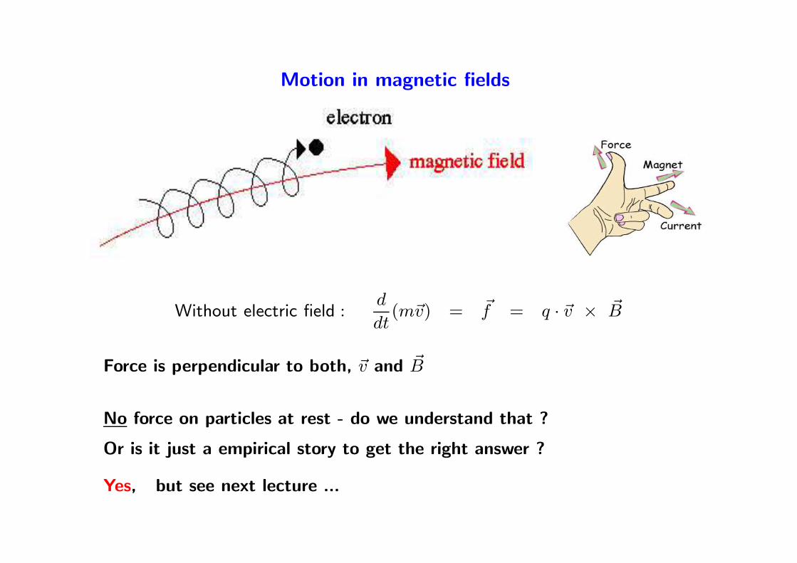
Motion in magnetic fields
Without electric field :d
dt(m~v) = ~f = q · ~v × ~B
Force is perpendicular to both, ~v and ~B
No force on particles at rest - do we understand that ?
Or is it just a empirical story to get the right answer ?
Yes, but see next lecture ...

Important application:
Tracks from particle collisions, lower energy particles have smaller
bending radius, allows determination of momenta ..
Q1: what is the direction of the magnetic field ???
Q2: what is the charge of the incoming particle ???

Practical units:
B [T ] · ρ [m] =p [eV/c]
c [m/s]
Example LHC:
B = 8.33 T, p = 712 eV/c ρ = 2804 m
More - bending angle α of a dipole magnet of length L:
α =B [T ] · L [m] · 0.3
p [GeV/c]
Example LHC:
B = 8.33 T, p = 7000 GeV/c, L = 14.3 m α = 5.11 mrad

... and some really strong magnetic fields
Example : CXOUJ164710.2− 45516
Diameter : 10 − 20 km
Field : ≈ 1012 Tesla
As accelerator : ≈ 1012 TeV
Very fast time varying electromagnetic fields - γ-ray bursts up to 1040 W
(sun: ≈ 4 · 1026 W)
Punchline:
Grand Unification (world formula) may show up near 1012 TeV

Time Varying Fields - (Maxwell 1864)
electricfield
electricfield
electricfield
magneticfield
magneticfield
magneticfield
AC current
propagationdirection of
Time varying magnetic fields produce circular electric fields
Time varying electric fields produce circular magnetic fields
Can produce self-sustaining, propagating fields (i.e. waves)
Rather useful picture in the classical framework, but ...

In vacuum: only fields, no charges (ρ = 0), no current (j = 0) ...
From Maxwell’s (III and IV) and some educated guess:
∇× (∇× ~B) = ∇2 ~E = −∇× (∂ ~B
∂t) = − ∂
∂t(∇× ~B)
=⇒ ∇2 ~E =∂
∂t
(
µ0ǫ0∂ ~E
∂t
)
= µ0ǫ0∂2 ~E
∂t2
∇2 ~E = µ0 · ǫ0 ·∂2 ~E
∂t2=
1
c2∂2 ~E
∂t2(correspondingly for ~B)
Equation for a wave with speed: c =1√
µ0 · ǫ0
It has a different form for a resting and a moving system !!!
see lecture on Special Relativity why and how it saves the day ...

Electromagnetic waves
~E = ~E0ei(ωt−~k·~x)
~B = ~B0ei(ωt−~k·~x)
Important quantities :
~k = (propagation vector)
λ = (wave length, 1 cycle)
ω = (frequency · 2π)~k · ~k =
ω2
c2(Dispersion Relation)
Magnetic and electric fields are transverse to direction of propagation:~E ⊥ ~B ⊥ ~k
Short wave length → high frequency → high energy

Spectrum of Electromagnetic waves
Example: yellow light ≈ 5 · 1014 Hz (i.e. ≈ 2 eV !)
LEP (SR) ≤ 2 · 1020 Hz (i.e. ≈ 0.8 MeV !)
gamma rays ≥ 3 · 1020 Hz (1 MeV to 10 TeV !)
(For estimates using temperature: 2.71 K ≈ 0.00023 eV )

Modulated wave: Group velocity and Phase velocity
-2
-1.5
-1
-0.5
0
0.5
1
1.5
2
0 50 100 150 200
phase velocity
group velocity
carrier wave :
vp =ω
k(phase velocity)
wave packet :
vg =∂ω
∂k(group velocity)
Wave packet can be considered as superposition of a number of
harmonic waves
Carrier wave moves at phase velocity, can be larger the c
Wave packet moves at group velocity, carries information
vp and vg may or may not be equal depends on ”dispersion relation”

Energy in electromagnetic waves (in brief, details in [2, 3, 4]):
define Poynting vector : ~S =1
µ0
~E × ~B (in direction of propagation)
”Energy flux”: energy crossing a unit area, per second [J
m2s]
In free space: energy is shared between electric and magnetic field
The energy density U would be:
UEB =1
2
(
ǫ0E2 +
1
µ0B2
)
Some example: B = 5·10−5 T ( = 0.5 Gauss)
UB ≈ 1 mJ/m3 (corresponds to ≈ 1016 γs at visible light)
Classical Electrodynamics is a very good approximation ..

Waves interacting with material
Need to look at the behaviour of electromagnetic fields at
boundaries between different materials (air-glass, air-water,
vacuum-metal, ...).
Have to consider two particular cases:
Ideal conductor (i.e. no resistance), apply to:
- RF cavities
- Wave guides
Conductor with finite resistance, apply to:
- Penetration and attenuation of fields in material (skin depth)
- Impedance calculations
Can be derived from Maxwell’s equations, here only the results !

Boundary conditions: air/vacuum and conductor
A simple case ( ~E-fields on a conducting surface):
En
n
n n n
E EE
nE
vector normal to boundary:
Field parallel to surface E‖ cannot exist (it would move charges and we
get a surface current): E‖ = 0
Only a field normal (orthogonal) to surface En is possible

Extreme case: surface of ideal conductor
For an ideal conductor (i.e. no resistance) the tangential electric field
must vanish Corresponding conditions for normal magnetic fields. We
must have:
~Et = 0, ~Bn = 0
This implies:
Fields at any point in the conductor are zero.
Only some field patterns are allowed in waveguides and RF cavities
A very nice lecture in R.P.Feynman, Vol. II
Now for Boundary Conditions between two different regions

Boundary conditions for electric fields
ε1 ε2µ1 µ2
Material 1 Material 2
E
E
t
n
ε1 ε2µ1 µ2
Material 1 Material 2
D
D
t
n
Assuming no surface charges (proof e.g. [3, 5])∗:
From curl ~E = 0:
tangential ~E-field continuous across boundary (E1t = E2
t )
From div ~D = ρ:
normal ~D-field continuous across boundary (D1n = D2
n)
∗with surface charges, see backup slides

Boundary conditions for magnetic fields
ε1 ε2µ1 µ2
Material 1 Material 2
n
tH
H
ε1 ε2µ1 µ2
Material 1 Material 2
B
B
t
n
Assuming no surface currents (proof e.g. [3, 5])∗:
From curl ~H = ~j:
tangential ~H-field continuous across boundary (H1t = H2
t )
From div ~B = 0:
normal ~B-field continuous across boundary (B1n = B2
n)
∗with surface current, see backup slides

Summary: boundary conditions for fields
Electromagnetic fields at boundaries between different materials with
different permittivity and permeability (ǫ1, ǫ2, µ1, µ2).
(E1t = E2
t ), (E1n 6= E2
n) or : ( ~E2 − ~E1) × ~n = 0
(D1t 6= D2
t ), (D1n = D2
n) or : ( ~D2 − ~D1) · ~n = ρsurface
(H1t = H2
t ), (H1n 6= H2
n) or : ( ~H2 − ~H1) × ~n = ~Jsurface
(B1t 6= B2
t ), (B1n = B2
n) or : ( ~B2 − ~B1) · ~n = 0
where ~n is the unit vector pointing into medium 2
(derivation deserves its own lectures, just believe it)
They determine: reflection, refraction and refraction index n.

Waves in material Index of refraction: n
Speed of electromagnetic waves in vacuum: c =1
√µ0 · ǫ0
n =Speed of light in vacuum
Speed of light in material=
c
vp
For water n ≈ 1.33
Depends on wavelength
n ≈ 1.32 − 1.39
some others ice: 1.31
alcohol: 1.36
sugar solution: 1.49
glass: 1.51
(propose an experiment !)

Reflection and refraction angles related to the refraction index n and n’:
µ’ε ’n’ =
µεn =
z
x
reflected waveincident wave
refracted wave
β
α
sin α
sin β=
n′
n= tan αB
If light is incident under angle αB [3]:
Reflected light is linearly polarized perpendicular to plane of incidence
(Application: fishing air-water gives αB ≈ 53o)
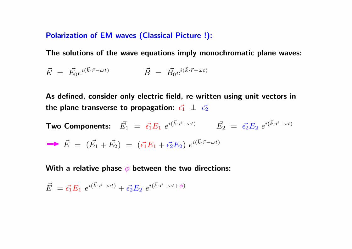
Polarization of EM waves (Classical Picture !):
The solutions of the wave equations imply monochromatic plane waves:
~E = ~E0ei(~k·~r−ωt) ~B = ~B0e
i(~k·~r−ωt)
As defined, consider only electric field, re-written using unit vectors in
the plane transverse to propagation: ~ǫ1 ⊥ ~ǫ2
Two Components: ~E1 = ~ǫ1E1 ei(~k·~r−ωt) ~E2 = ~ǫ2E2 ei(
~k·~r−ωt)
~E = ( ~E1 + ~E2) = (~ǫ1E1 + ~ǫ2E2) ei(~k·~r−ωt)
With a relative phase φ between the two directions:
~E = ~ǫ1E1 ei(~k·~r−ωt) + ~ǫ2E2 ei(
~k·~r−ωt+φ)

Ey Ey
EyEy
Ey
Ex Ex
Ex Ex
Ex
linear : E2 = 0 or E1 = 0
circular : φ ± π
2
elliptical : φ e.g.π
4

Polarized light - why is it interesting:
Produced (amongst others) in Synchrotron light machines (linearly and circularly
polarized light, adjustable) blue sky (!), reflections (e.g. water surface)
Accelerator and other applications:
Polarized light reacts differently with charged particles
Radio communication, capacity doubling
Beam diagnostics, medical diagnostics (blood sugar, ..)
Inverse FEL
3-D motion pictures, LCD display, cameras (reduce glare)
Outdoor activities (e.g. Fishing, driving a car through a rainy night, ... )
...
Less classical, in Quantum Electro Dynamics: photons with spin +1 or -1

Practical application:
Some of the light is reflected
Some of the light is transmitted and refracted
For αB, can be largely supressed using polarised glasses

Extreme case: ideal conductor
For an ideal conductor (i.e. no resistance) we must have:
~E‖ = 0, ~Bn = 0
otherwise the surface current becomes infinite
This implies:
All energy of an electromagnetic wave is reflected from the surface
of an ideal conductor.
Fields at any point in the ideal conductor are zero.
Only some fieldpatterns are allowed in waveguides and RF cavities
A very nice lecture in R.P.Feynman, Vol. II

Examples: cavities and wave guides
Rectangular, conducting cavities and wave guides (schematic) with
dimensions a× b× c and a× b:x
y
z
a
b
c
x
y
z
a
b
RF cavity, fields can persist and be stored (reflection !)
Plane waves can propagate along wave guides, here in z-direction
(here just the basics, many details in ”RF Systems” by Frank Tecker)

Fields in RF cavities - as reference
Assume a rectangular RF cavity (a, b, c), ideal conductor.
Without derivations, the components of the fields are:
Ex = Ex0 · cos(kxx) · sin(kyy) · sin(kzz) · e−iωt
Ey = Ey0 · sin(kxx) · cos(kyy) · sin(kzz) · e−iωt
Ez = Ez0 · sin(kxx) · sin(kyy) · cos(kzz) · e−iωt
Bx =i
ω(Ey0kz − Ez0ky) · sin(kxx) · cos(kyy) · cos(kzz) · e−iωt
By =i
ω(Ez0kx − Ex0kz) · cos(kxx) · sin(kyy) · cos(kzz) · e−iωt
Bz =i
ω(Ex0ky − Ey0kx) · cos(kxx) · cos(kyy) · sin(kzz) · e−iωt
-2
-1.5
-1
-0.5
0
0.5
1
1.5
2
0 0.2 0.4 0.6 0.8 1
dimension a
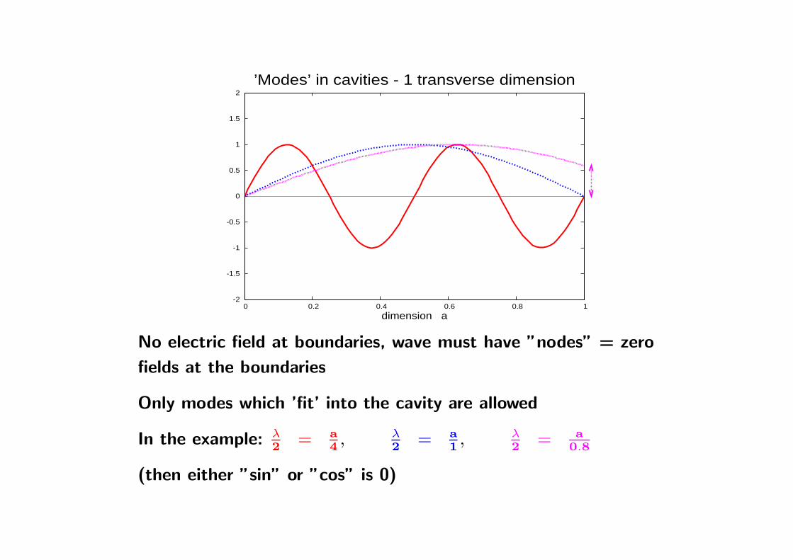
’Modes’ in cavities - 1 transverse dimension
No electric field at boundaries, wave must have ”nodes” = zero
fields at the boundaries
Only modes which ’fit’ into the cavity are allowed
In the example: λ2
= a
4, λ
2= a
1, λ
2= a
0.8
(then either ”sin” or ”cos” is 0)

Consequences for RF cavities
Field must be zero at conductor boundary, only possible if:
k2x + k2
y + k2z =
ω2
c2
and for kx, ky, kz we can write, (then they all fit):
kx =mxπ
a, ky =
myπ
b, kz =
mzπ
c,
The integer numbers mx,my,mz are called mode numbers, important for
design of cavity !
→ half wave length λ/2 must always fit exactly the size of the cavity.
(For cylindrical cavities: use cylindrical coordinates )

Wave guides and cavities are more likely to be circular:
Derivation using the Laplace equation in cylindrical coordinates, for a
derivation see e.g. [2, 3]:
Er = E0kzkr
J ′n(kr) · cos(nθ) · sin(kzz) · e−iωt
Eθ = E0nkzk2rr
Jn(kr) · sin(nθ) · sin(kzz) · e−iωt
Ez = E0 Jn(krr) · cos(nθ) · sin(kzz) · e−iωt
Br = iE0ω
c2k2rr
Jn(krr) · sin(nθ) · cos(kzz) · e−iωt
Bθ = iE0ω
c2krrJ ′n(krr) · cos(nθ) · cos(kzz) · e−iωt
Bz = 0
Homework: write it down for wave guides ..
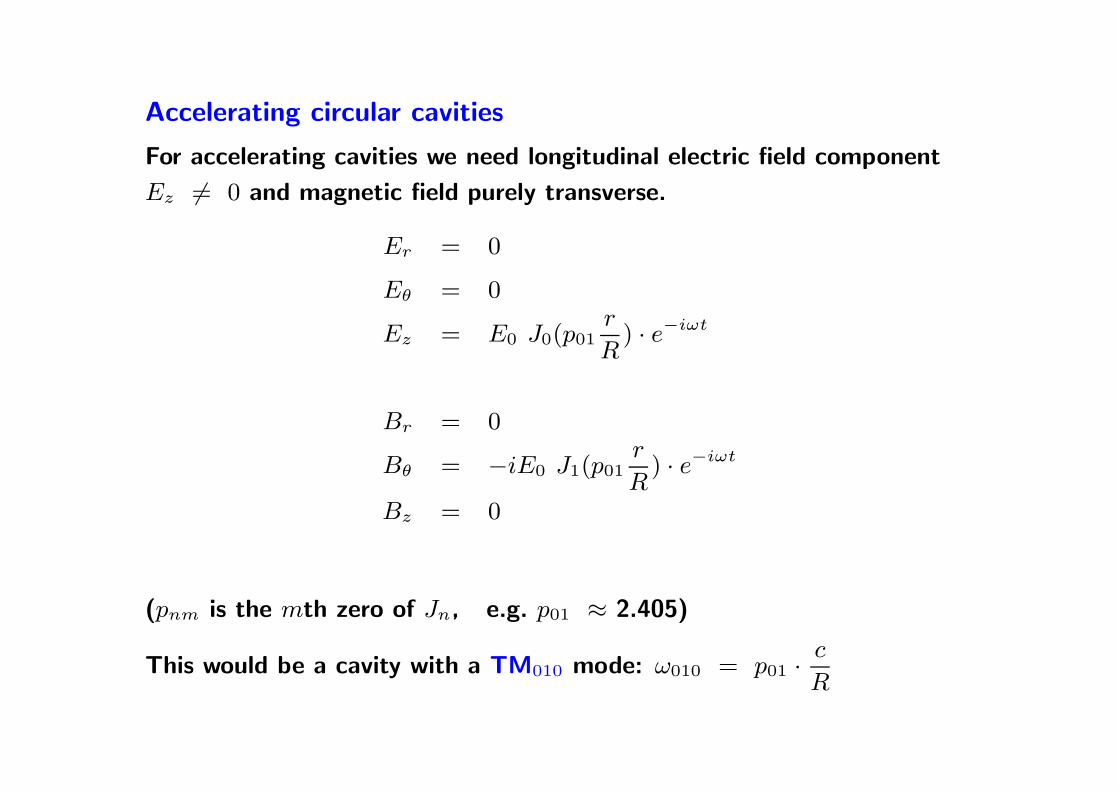
Accelerating circular cavities
For accelerating cavities we need longitudinal electric field component
Ez 6= 0 and magnetic field purely transverse.
Er = 0
Eθ = 0
Ez = E0 J0(p01r
R) · e−iωt
Br = 0
Bθ = −iE0 J1(p01r
R) · e−iωt
Bz = 0
(pnm is the mth zero of Jn, e.g. p01 ≈ 2.405)
This would be a cavity with a TM010 mode: ω010 = p01 ·c
R

Similar considerations lead to (propagating) solutions in (rectangular)
wave guides:
Ex = Ex0 · cos(kxx) · sin(kyy) · ei(kzz−ωt)
Ey = Ey0 · sin(kxx) · cos(kyy) · ei(kzz−ωt)
Ez = i · Ez0 · sin(kxx) · sin(kyy) · ei(kzz−ωt)
Bx =1
ω(Ey0kz − Ez0ky) · sin(kxx) · cos(kyy) · ei(kzz−ωt)
By =1
ω(Ez0kx − Ex0kz) · cos(kxx) · sin(kyy) · ei(kzz−ωt)
Bz =1
i · ω (Ex0ky − Ey0kx) · cos(kxx) · cos(kyy) · ei(kzz−ωt)
This part is new: ei(kzz) =⇒ something moving in z direction
In z direction: No Boundary - No Boundary Condition ...

Consequences for wave guides
Similar considerations as for cavities, no field at boundary.
We must satisfy again the condition:
k2x + k2
y + k2z =
ω2
c2=⇒ kz =
√
ω2
c2− k2
x − k2y
This leads to modes like (no boundaries in direction of propagation,
only kx and ky have to ”fit”):
kx =mxπ
a, ky =
myπ
b, kz =
√
ω2
c2−(mxπ
a
)2
−(myπ
b
)2
The numbers mx,my are called mode numbers for waves in wave guides !
Should we worry about kz ?? Argument of root can become negative .. !

Propagation without losses requires kz to be real, i.e.:
ω2
c2>(mxπ
a
)2
+(myπ
b
)2
ω > πc
√(mx
a
)2
+(my
b
)2
defines a (minimum) cut-off frequency ωc:
ωc =π · ca
(with a the longest side length of the wave guide)
Above cut-off frequency: propagation without loss
At cut-off frequency: standing wave
Below cut-off frequency: attenuated wave (it does not ”fit in”).
(if bored : try to compute vp and vg for the limits : ω → ∞ and ω → ωc)

Classification of modes:
Transverse electric modes (TE): Ez = 0 Hz 6= 0
Transverse magnetic modes (TM): Ez 6= 0 Hz = 0
Transverse electric-magnetic modes (TEM): Ez = 0 Hz = 0
(Not all of them can be used for acceleration ... !)
B
E
Note (here a TE mode) :
Electric field lines end at boundaries
Magnetic field lines appear as ”loops”

Other case: finite conductivity
Starting from Maxwell equation:
∇× ~B = µ~j + µǫd ~E
dt=
~j︷ ︸︸ ︷
σ · ~E︸ ︷︷ ︸
Ohm′s law
+ µǫd ~E
dt
Wave equations:
~E = ~E0ei(~k·~r−ωt), ~B = ~B0e
i(~k·~r−ωt)
We want to know k with this new contribution:
k2 =ω2
c2− iωσµ︸ ︷︷ ︸
new

Consequence Skin Depth
Electromagnetic waves can now penetrate into the conductor !
For a good conductor σ ≫ ωǫ:
k2 ≈ − iωµσ k ≈√
ωµσ
2(1 + i) =
1
δ(1 + i)
δ =
√
2
ωµσis the Skin Depth
High frequency waves ”avoid” penetrating into a conductor,
flow near the surface
Penetration depth small for large conductivity

”Explanation” - inside a conductor (very schematic)
IeIe
Ie Ie
HI
add current
subtract current
Eddy currents IE from changing ~H-field: ∇× ~E = µ0d ~H
dt
Cancel current flow in the centre of the conductor I − Ie
Enforce current flow near the ”skin” (surface) I + Ie
Q: Why are high frequency cables thin ??

Attenuated waves - penetration depth
1e-10
1e-08
1e-06
0.0001
0.01
1
100
1 100 10000 1e+06 1e+08 1e+10 1e+12 1e+14 1e+16
skin
dep
th (
m)
Frequency (Hz)
Skin Depth versus frequencyCopper
Gold Stainless steel
Carbon (amorphous)
Waves incident on conducting
material are attenuated
Basically by the Skin depth :
(attenuation to 1/e)
δ =
√2
ωµσ
Wave form:
ei(kz−ωt) = ei((1+i)z/δ−ωt) = e−zδ · ei( z
δ−ωt)
Values of δ can have a very large range ..

Skin depth Copper (σ ≈ 6 · 107 S/m):
2.45 GHz: δ ≈ 1.5 µm, 50 Hz: δ ≈ 10 mm
Penetration depth Glass (strong variation, σ typically 6 · 10−13 S/m):
2.45 GHz: δ > km
Penetration depth Sushi (strong variation, σ typically 3 · 10−2 S/m):
2.45 GHz: δ ≈ 6 cm
Penetration depth Seawater (σ ≈ 4 S/m):
76 Hz: δ ≈ 25 - 30 m (Design an antenna !!, very low bandwidth)

Done list:
1. Review of basics and write down Maxwell’s equations
2. Electromagnetic fields in vacuum and in material
3. Add Lorentz force and motion of particles in EM fields
4. Electromagnetic waves in vacuum
5. Electromagnetic waves in conducting media
Waves in RF cavities
Waves in wave guides
Important concepts: mode numbers, cut-off frequency, skin
depth
But still a few (important) problems to sort out

What next:
We have to deal with moving charges in accelerators
Applied to moving charges Maxwell’s equations are not compatible with
observations of electromagnetic phenomena
Electromagnetism and laws of classical mechanics are inconsistent
Ad hoc introduction of Lorentz force
Electromagnetic ”wave” concept is fuzzy: no medium (more in lecture on
Special Relativity)
Needed: sort in out in a systematic framework
The fix: Special Relativity (next lecture)
Formulate Maxwell’s equations relativistically invariant
Problems solved (easily !) ...

- BACKUP SLIDES -

Relativity and electrodynamics
- Back to the start: electrodynamics and Maxwell equations
- Life made easy with four-vectors ..
- Strategy: one + three
Write potentials and currents as four-vectors:
Ψ, ~A ⇒ Aµ = (Ψ
c, ~A)
ρ, ~j ⇒ Jµ = (ρ · c, ~j)
What about the transformation of current and potentials ?

Transform the four-current like:
ρ′c
j′x
j′y
j′z
=
γ −γβ 0 0
−γβ γ 0 0
0 0 1 0
0 0 0 1
ρc
jx
jy
jz
It transforms via: J ′µ = Λ Jµ (always the same Λ)
Ditto for: A′µ = Λ Aµ (always the same Λ)
Note: ∂µJµ =
∂ρ
∂t+ ~∇~j = 0 (charge conservation)

Electromagnetic fields using potentials:
Magnetic field: ~B = ∇× ~A
e.g. the x-component:
Bx =∂A3
∂y− ∂A2
∂z=
∂Az
∂y− ∂Ay
∂z
Electric field: ~E = −∇Ψ − ∂ ~A
∂t
e.g. for the x-component:
Ex = − ∂A0
∂x− ∂A1
∂t= − ∂At
∂x− ∂Ax
∂t
after getting all combinations ..

Electromagnetic fields described by field-tensor Fµν :
Fµν = ∂µAν − ∂νAµ =
0−Ex
c
−Ey
c
−Ez
c
Ex
c0 −Bz By
Ey
cBz 0 −Bx
Ez
c−By Bx 0
It transforms via: F ′µν = Λ Fµν ΛT (same Λ as before)
(Warning: There are different ways to write the field-tensor Fµν ,
I use the convention from [1, 3, 5])

Transformation of fields into a moving frame (x-direction):
Use Lorentz transformation of Fµν and write for components:
E′x = Ex B′
x = Bx
E′y = γ(Ey − v ·Bz) B′
y = γ(By +vc2
· Ez)
E′z = γ(Ez + v ·By) B′
z = γ(Bz − vc2
· Ey)
Fields perpendicular to movement are transformed

Example Coulomb field: (a charge moving with constant speed)
γ = 1 γ >> 1
In rest frame purely electrostatic forces
In moving frame ~E transformed and ~B appears
How do the fields look like ?
Needed to compute e.g. radiation of a moving charge, wake
fields, ...

For the static charge we have the Coulomb potential (see lecture
on Electrodynamics) and ~A = 0
Transformation into the new frame (moving in x-direction) with
our transformation of four-potentials:
Ψ′
c= γ(
Ψ
c−Ax) = γ
Ψ
c
A′
x = γ
(
Ax − vΨ
c2
)
= −γv
c2Ψ = − v
c2Ψ′
i.e. all we need to know is Ψ′
Ψ′(~r) = γΨ(~r) = γ · 1
4πǫ0· q
|~r − ~rq|
After transformation of coordinates, e.g. x = γ(x′ − vt′)
The resulting potentials can be used to compute the fields.

Watch out !!
We have to take care of causality:
The field observed at a position ~r at time t was caused at an
earlier time tr < t at the location ~r0(tr)
Ψ(~r, t) =qc
|~R|c− ~R~v~A(~r, t) =
q~v
|~R|c− ~R~v
The potentials Ψ(~r, t) and ~A(~r, t) depend on the state at retarted
time tr, not t
~v is the velocity at time tr and ~R = ~r − ~r0(tr) relates the
retarted position to the observation point.
Q: Can we also write a Four-Maxwell ?

Re-write Maxwell’s equations using four-vectors and Fµν :
∇ ~E =ρ
ǫ0and ∇× ~B − 1
c2∂ ~E
∂t= µ0
~J1+3
∂µFµν = µ0J
ν (Inhomogeneous Maxwell equation)
∇ ~B = 0 and ∇× ~E +∂ ~B
∂t= 0
1+3
∂γFµν + ∂µF
νλ + ∂νFλµ = 0 (Homogeneous Maxwell equation)
We have Maxwell’s equation in a very compact form,
transformation between moving systems very easy

How to use all that stuff ??? Look at first equation:
∂µFµν = µ0J
ν
Written explicitly (Einstein convention, sum over µ):
∂µFµν =
3∑
µ=0
∂µFµν = ∂0F
0ν + ∂1F1ν + ∂2F
2ν + ∂3F3ν = µ0J
ν
Choose e.g. ν = 0 and replace Fµν by corresponding elements:
∂0F00 + ∂1F
10 + ∂2F20 + ∂3F
30 = µ0J0
0 + ∂xEx
c+ ∂y
Ey
c+ ∂z
Ez
c= µ0J
0 = µ0 cρ
This corresponds exactly to:
~∇ · ~E =ρ
ǫ0(c2 = ǫ0µ0)

For ν = 1, 2, 3 you get Ampere’s law
For example in the x-plane (ν = 1) and the S frame:
∂yBz − ∂zBy − ∂tEx
c= µ0J
x
after transforming ∂γ and Fµν to the S’ frame:
∂′
yB′
z − ∂′
zB′
y − ∂′
t
E′x
c= µ0J
′x
Now Maxwell’s equation have the identical form in S and S’
(In matter: can be re-written with ~D and ~H using
”magnetization tensor”)

Finally: since Fµν = ∂µAν − ∂νAµ
∂µFµν = µ0J
ν
∂γFµν + ∂µF
νλ + ∂νFλµ = 0
We can re-write them two-in-one in a new form:
∂2Aµ
∂xν∂xν= µ0J
µ
This contains all four Maxwell’s equations, and the only one
which stays the same in all frames !!
There are no separate electric and magnetic fields, just a frame
dependent manifestation of a single electromagnetic field
Quite obvious in Quantum ElectroDynamics !