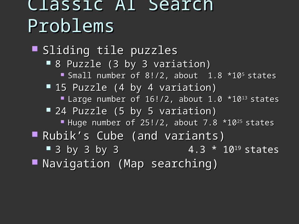
Classic AI Search Problems Sliding tile puzzles Sliding tile puzzles 8 Puzzle (3 by 3 variation) 8...
43
Classic AI Search Classic AI Search Problems Problems Sliding tile puzzles Sliding tile puzzles 8 Puzzle (3 by 3 variation) 8 Puzzle (3 by 3 variation) Small number of 8!/2, about 1.8 *10 Small number of 8!/2, about 1.8 *10 5 5 states states 15 Puzzle (4 by 4 variation) 15 Puzzle (4 by 4 variation) Large number of 16!/2, about 1.0 *10 Large number of 16!/2, about 1.0 *10 13 13 states states 24 Puzzle (5 by 5 variation) 24 Puzzle (5 by 5 variation) Huge number of 25!/2, about 7.8 *10 Huge number of 25!/2, about 7.8 *10 25 25 states states Rubik’s Cube (and variants) Rubik’s Cube (and variants) 3 by 3 by 3 3 by 3 by 3 4.3 * 10 19 states Navigation (Map searching) Navigation (Map searching)
-
Upload
elian-gallon -
Category
Documents
-
view
232 -
download
0
Transcript of Classic AI Search Problems Sliding tile puzzles Sliding tile puzzles 8 Puzzle (3 by 3 variation) 8...
Classic AI Search ProblemsClassic AI Search Problems Sliding tile puzzlesSliding tile puzzles
8 Puzzle (3 by 3 variation) 8 Puzzle (3 by 3 variation) Small number of 8!/2, about 1.8 *10Small number of 8!/2, about 1.8 *105 5 states states
15 Puzzle (4 by 4 variation)15 Puzzle (4 by 4 variation) Large number of 16!/2, about 1.0 *10Large number of 16!/2, about 1.0 *1013 13 statesstates
24 Puzzle (5 by 5 variation) 24 Puzzle (5 by 5 variation) Huge number of 25!/2, about 7.8 *10Huge number of 25!/2, about 7.8 *1025 25 statesstates
Rubik’s Cube (and variants)Rubik’s Cube (and variants) 3 by 3 by 3 3 by 3 by 3 4.3 * 1019 states
Navigation (Map searching)Navigation (Map searching)
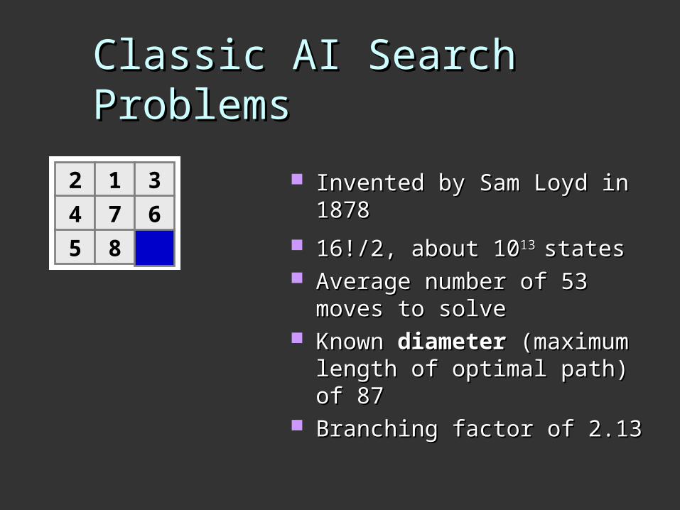
Classic AI Search ProblemsClassic AI Search Problems
Invented by Sam Loyd in Invented by Sam Loyd in 18781878
16!/2, about 1016!/2, about 1013 13 statesstates Average number of 53 Average number of 53
moves to solvemoves to solve Known Known diameterdiameter (maximum (maximum
length of optimal path) of 87length of optimal path) of 87 Branching factor of 2.13 Branching factor of 2.13
2 1 3
4 7 6
5 8
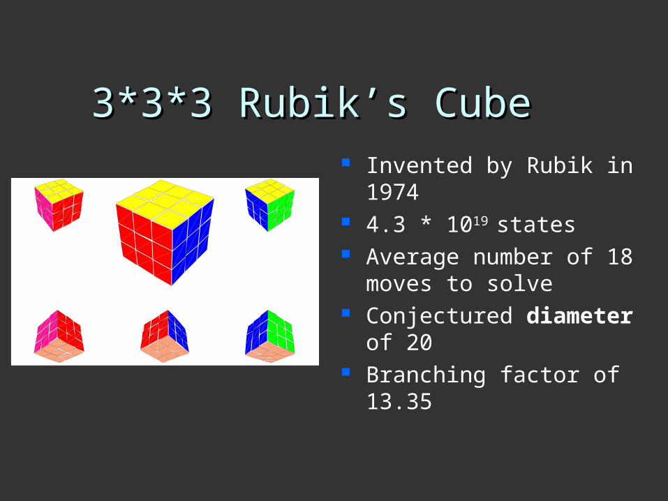
3*3*3 Rubik’s Cube3*3*3 Rubik’s Cube Invented by Rubik in
1974 4.3 * 1019 states Average number of 18
moves to solve Conjectured diameter
of 20 Branching factor of
13.35
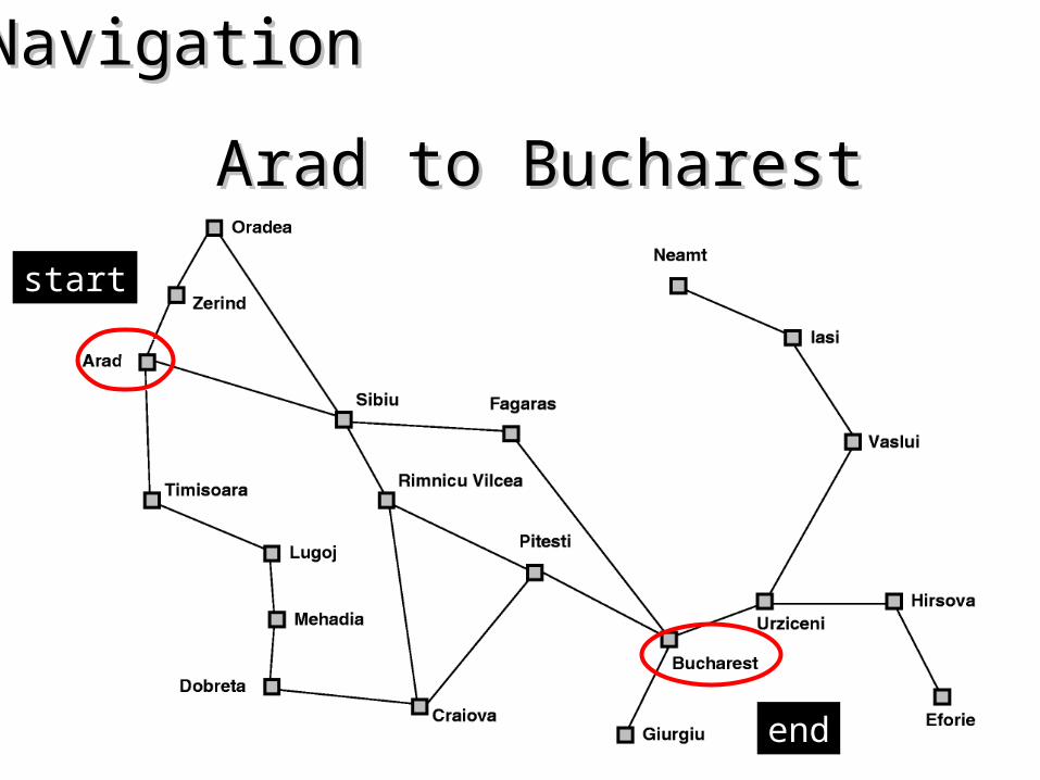
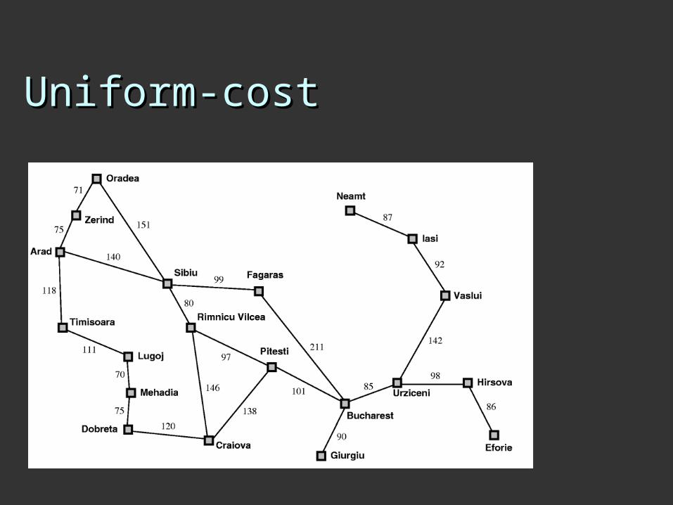
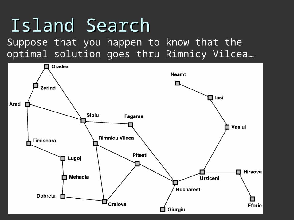
Arad to BucharestArad to Bucharest
start
end
NavigationNavigation
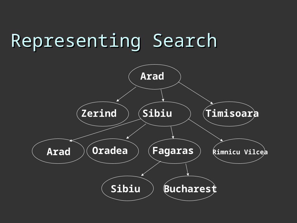
Representing SearchRepresenting Search
Arad
Zerind Sibiu Timisoara
Oradea Fagaras Rimnicu VilceaArad
Sibiu Bucharest
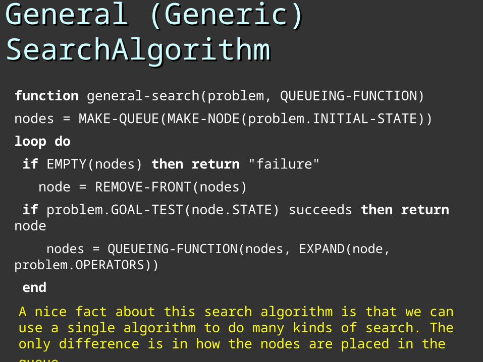
General (Generic) General (Generic) SearchAlgorithm SearchAlgorithm
function general-search(problem, QUEUEING-FUNCTION)
nodes = MAKE-QUEUE(MAKE-NODE(problem.INITIAL-STATE))
loop do
if EMPTY(nodes) then return "failure"
node = REMOVE-FRONT(nodes)
if problem.GOAL-TEST(node.STATE) succeeds then return node
nodes = QUEUEING-FUNCTION(nodes, EXPAND(node, problem.OPERATORS))
end
A nice fact about this search algorithm is that we can use a single algorithm to do many kinds of search. The only difference is in how the nodes are placed in
the queue.
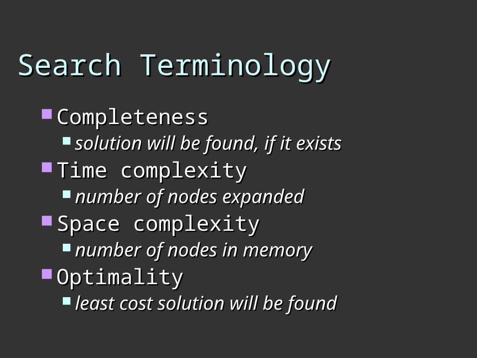
Search TerminologySearch Terminology
CompletenessCompleteness solution will be found, if it existssolution will be found, if it exists
Time complexityTime complexity number of nodes expandednumber of nodes expanded
Space complexitySpace complexity number of nodes in memorynumber of nodes in memory
OptimalityOptimality least cost solution will be foundleast cost solution will be found
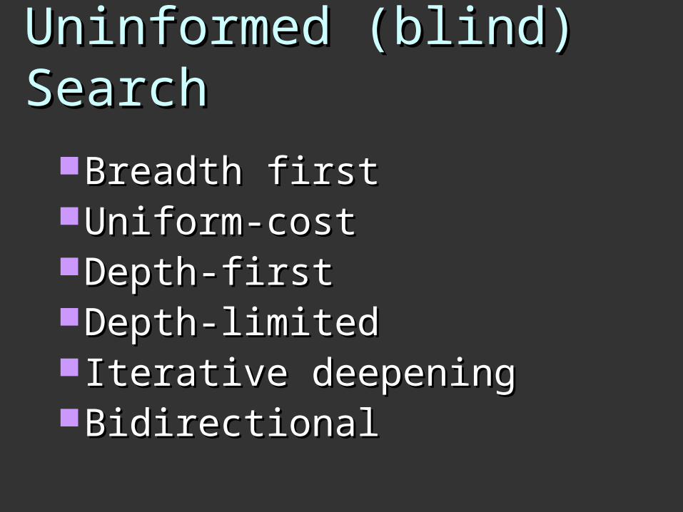
Uninformed (blind) Uninformed (blind) SearchSearch
Breadth firstBreadth firstUniform-costUniform-costDepth-firstDepth-firstDepth-limitedDepth-limited Iterative deepeningIterative deepeningBidirectional Bidirectional
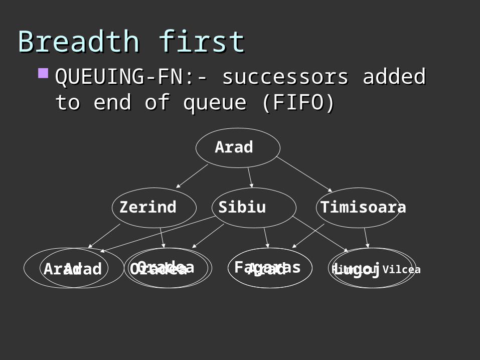
Breadth firstBreadth first QUEUING-FN:- successors added to QUEUING-FN:- successors added to
end of queue (FIFO)end of queue (FIFO)
Arad
Zerind Sibiu Timisoara
Oradea Fagaras Rimnicu VilceaAradArad Oradea Arad Lugoj
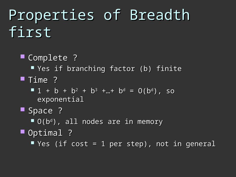
Properties of Breadth firstProperties of Breadth first
Complete ?Complete ? Yes if branching factor (b) finiteYes if branching factor (b) finite
Time ?Time ? 1 + b + b1 + b + b22 + b + b33 +…+ b +…+ bdd = O(b = O(bdd), so ), so
exponentialexponential Space ?Space ?
O(bO(bdd), all nodes are in memory), all nodes are in memory Optimal ?Optimal ?
Yes (if cost = 1 per step), not in generalYes (if cost = 1 per step), not in general
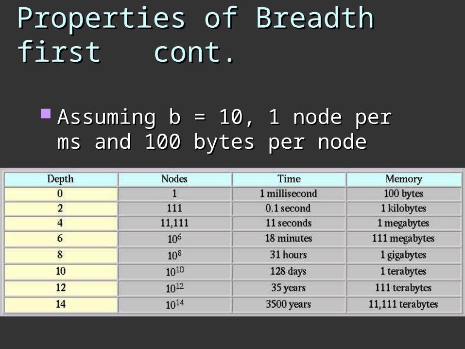
Properties of Breadth first Properties of Breadth first cont.cont.
Assuming b = 10, 1 node per ms Assuming b = 10, 1 node per ms and 100 bytes per nodeand 100 bytes per node
Uniform-costUniform-cost
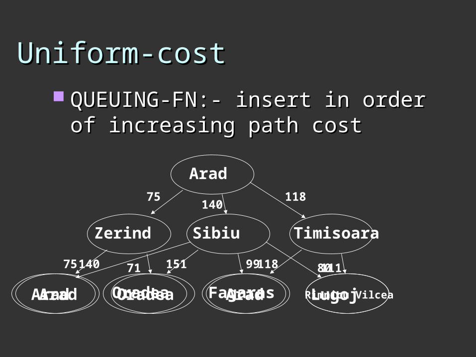
Uniform-costUniform-cost QUEUING-FN:- insert in order of QUEUING-FN:- insert in order of
increasing path cost increasing path cost
Arad
Zerind Sibiu Timisoara
75 118140
Oradea Fagaras Rimnicu VilceaArad
140 151 99 80
Arad Oradea
75 71
Arad Lugoj
118 111
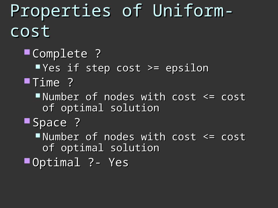
Properties of Uniform-costProperties of Uniform-cost Complete ?Complete ?
Yes if step cost >= epsilonYes if step cost >= epsilon Time ?Time ?
Number of nodes with cost <= cost of Number of nodes with cost <= cost of optimal solutionoptimal solution
Space ?Space ? Number of nodes with cost <= cost of Number of nodes with cost <= cost of
optimal solutionoptimal solution Optimal ?- YesOptimal ?- Yes
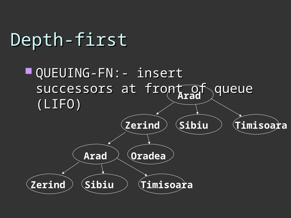
Depth-firstDepth-first
QUEUING-FN:- insert successors at QUEUING-FN:- insert successors at front of queue (LIFO)front of queue (LIFO)
Arad
Zerind Sibiu Timisoara
Arad Oradea
Zerind Sibiu Timisoara
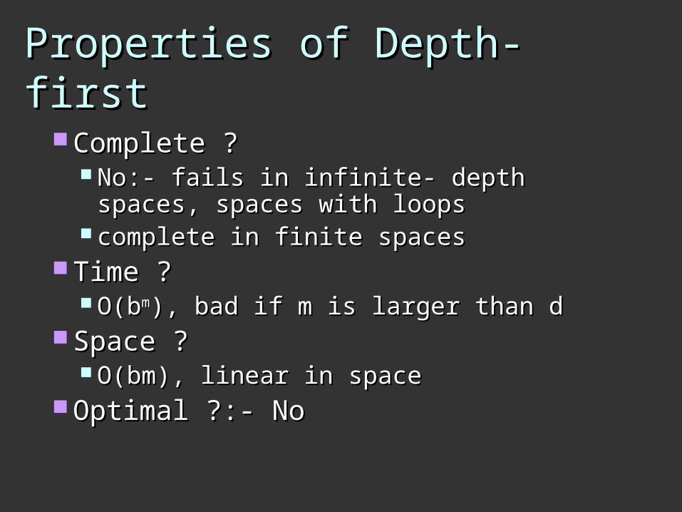
Properties of Depth-firstProperties of Depth-first Complete ?Complete ?
No:- fails in infinite- depth spaces, No:- fails in infinite- depth spaces, spaces with loopsspaces with loops
complete in finite spacescomplete in finite spaces Time ?Time ?
O(bO(bmm), bad if m is larger than d), bad if m is larger than d Space ?Space ?
O(bm), linear in spaceO(bm), linear in space Optimal ?:- NoOptimal ?:- No
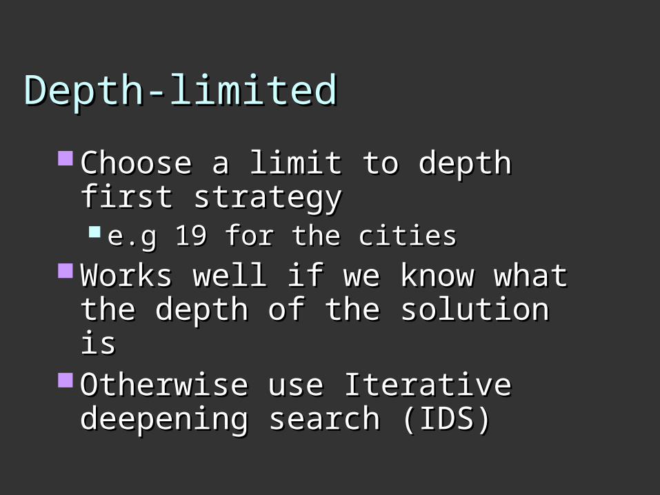
Depth-limitedDepth-limited
Choose a limit to depth first Choose a limit to depth first strategystrategy e.g 19 for the cities e.g 19 for the cities
Works well if we know what the Works well if we know what the depth of the solution isdepth of the solution is
Otherwise use Iterative Otherwise use Iterative deepening search (IDS)deepening search (IDS)
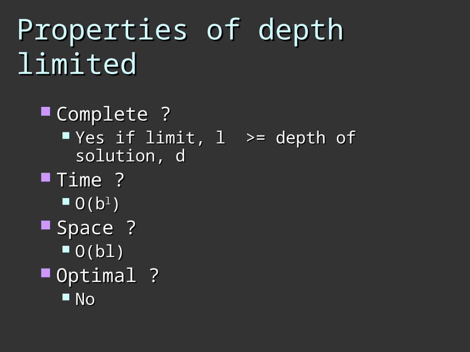
Properties of depth limitedProperties of depth limited
Complete ?Complete ? Yes if limit, l >= depth of solution, dYes if limit, l >= depth of solution, d
Time ?Time ? O(bO(bll))
Space ?Space ? O(bl)O(bl)
Optimal ?Optimal ? NoNo
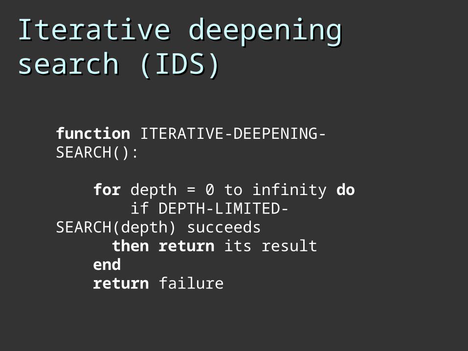
Iterative deepening search Iterative deepening search (IDS)(IDS)
function ITERATIVE-DEEPENING-SEARCH():
for depth = 0 to infinity do if DEPTH-LIMITED-SEARCH(depth) succeeds
then return its result end return failure
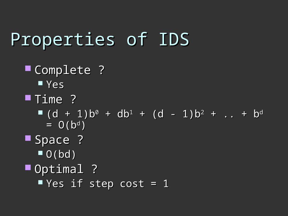
Properties of IDSProperties of IDS
Complete ?Complete ? YesYes
Time ?Time ? (d + 1)b(d + 1)b00 + db + db11 + (d - 1)b + (d - 1)b22 + .. + b + .. + bdd = =
O(bO(bdd)) Space ?Space ?
O(bd)O(bd) Optimal ?Optimal ?
Yes if step cost = 1Yes if step cost = 1
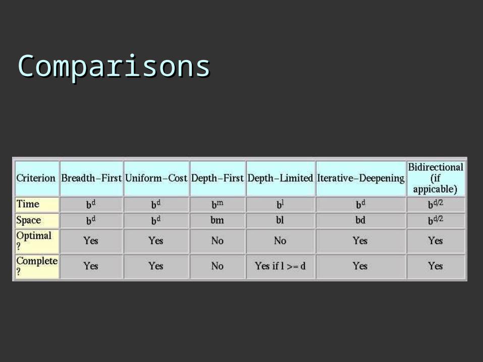
ComparisonsComparisons
Summary Summary
Various uninformed search Various uninformed search strategiesstrategies
Iterative deepening is linear in Iterative deepening is linear in spacespace not much more time than othersnot much more time than others
Use Bi-directional Iterative Use Bi-directional Iterative deepening were possible deepening were possible
Island Search Island Search Suppose that you happen to know that the optimal solution goes thru Rimnicy Vilcea…
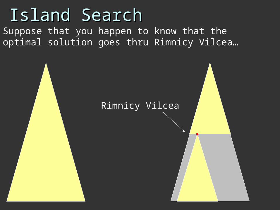
Island Search Island Search Suppose that you happen to know that the optimal solution goes thru Rimnicy Vilcea…
Rimnicy Vilcea
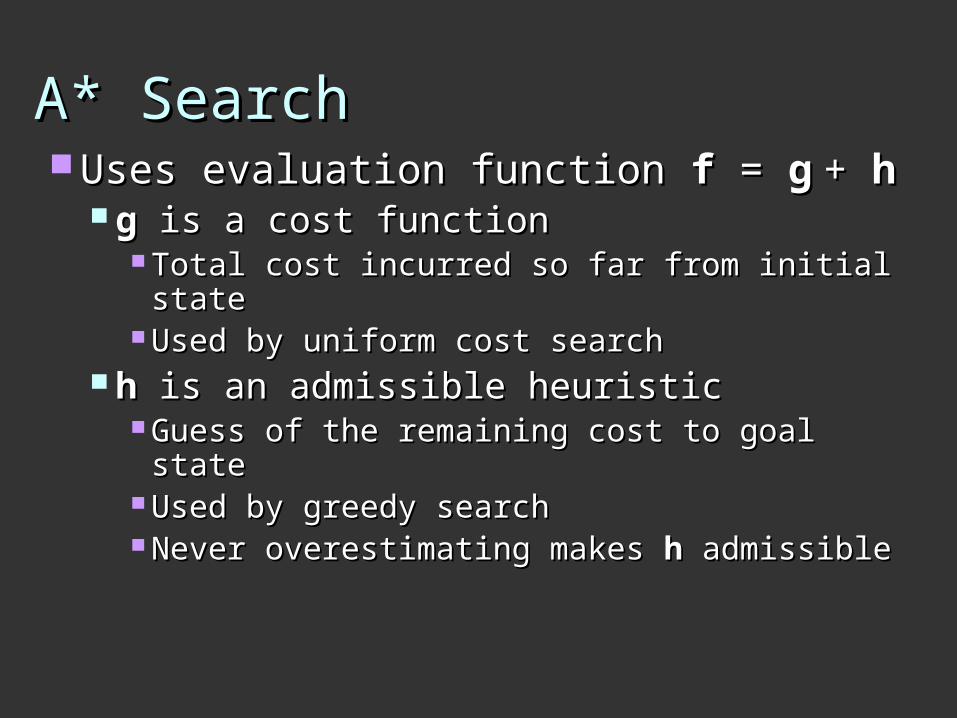
A* SearchA* Search Uses evaluation function Uses evaluation function f f == g g + + hh
g g is a cost functionis a cost function Total cost incurred so far from initial stateTotal cost incurred so far from initial state Used by uniform cost searchUsed by uniform cost search
h h is an admissible heuristicis an admissible heuristic Guess of the remaining cost to goal stateGuess of the remaining cost to goal state Used by greedy searchUsed by greedy search Never overestimating makes Never overestimating makes hh
admissibleadmissible
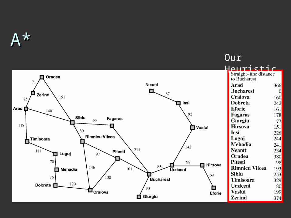
A*A*Our Heuristic
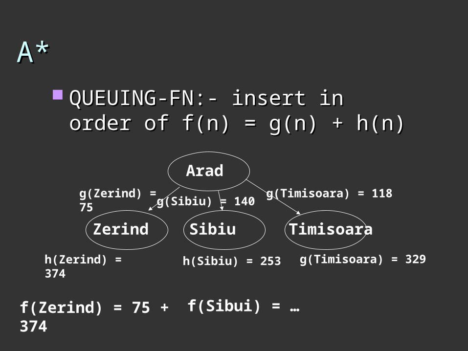
A*A* QUEUING-FN:- insert in order of QUEUING-FN:- insert in order of
f(n) = g(n) + h(n) f(n) = g(n) + h(n)
Arad
Zerind Sibiu Timisoara
g(Zerind) = 75 g(Timisoara) = 118g(Sibiu) = 140
h(Zerind) = 374 h(Sibiu) = 253 g(Timisoara) = 329
f(Zerind) = 75 + 374 f(Sibui) = …
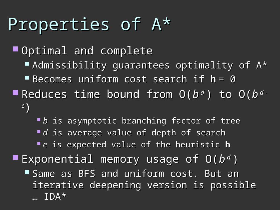
Properties of A*Properties of A* Optimal and completeOptimal and complete
Admissibility guarantees optimality of A*Admissibility guarantees optimality of A* Becomes uniform cost search if Becomes uniform cost search if hh = 0= 0
Reduces time bound from O(Reduces time bound from O(bb d d ) to O() to O(bb d - d -
ee)) bb is asymptotic branching factor of tree is asymptotic branching factor of tree dd is average value of depth of search is average value of depth of search ee is expected value of the heuristic is expected value of the heuristic hh
Exponential memory usage of O(Exponential memory usage of O(bb d d )) Same as BFS and uniform cost. But an Same as BFS and uniform cost. But an
iterative deepening version is possible … iterative deepening version is possible … IDA*IDA*
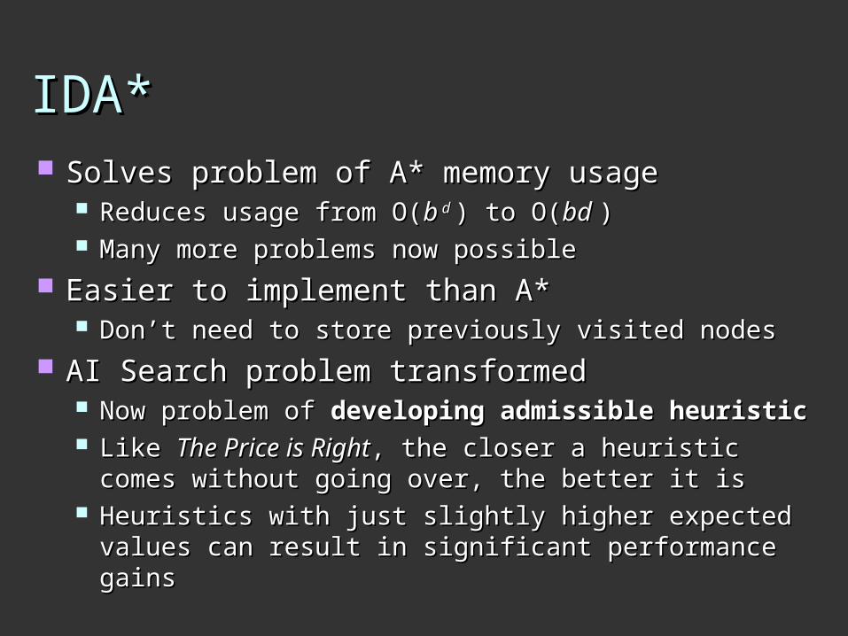
IDA*IDA* Solves problem of A* memory usageSolves problem of A* memory usage
Reduces usage from O(Reduces usage from O(bb d d ) to O() to O(bd bd )) Many more problems now possibleMany more problems now possible
Easier to implement than A*Easier to implement than A* Don’t need to store previously visited nodes Don’t need to store previously visited nodes
AI Search problem transformed AI Search problem transformed Now problem of Now problem of developing admissible developing admissible
heuristicheuristic Like Like The Price is RightThe Price is Right, the closer a heuristic , the closer a heuristic
comes without going over, the better it iscomes without going over, the better it is Heuristics with just slightly higher expected Heuristics with just slightly higher expected
values can result in significant performance gainsvalues can result in significant performance gains

A* “trick”A* “trick” Suppose you have two admissible Suppose you have two admissible
heuristics…heuristics… But h1(n) > h2(n)But h1(n) > h2(n) You may as well forget h2(n)You may as well forget h2(n)
Suppose you have two admissible Suppose you have two admissible heuristics…heuristics… Sometimes h1(n) > h2(n) and sometimes Sometimes h1(n) > h2(n) and sometimes
h1(n) < h2(n)h1(n) < h2(n) We can now define a better heuristic, h3 We can now define a better heuristic, h3 h3(n) = max( h1(n) , h2(n) )h3(n) = max( h1(n) , h2(n) )
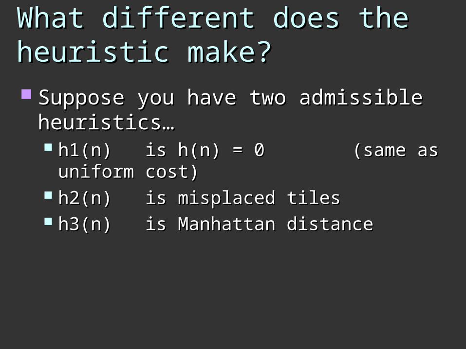
What different does the What different does the heuristic make?heuristic make? Suppose you have two admissible Suppose you have two admissible
heuristics…heuristics… h1(n) is h(n) = 0 (same as uniform h1(n) is h(n) = 0 (same as uniform
cost)cost) h2(n) is misplaced tilesh2(n) is misplaced tiles h3(n) is Manhattan distanceh3(n) is Manhattan distance
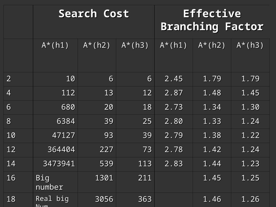
Search CostSearch Cost Effective Branching Effective Branching FactorFactor
A*(h1)A*(h1) A*(h2)A*(h2) A*(h3)A*(h3) A*(h1)A*(h1) A*(h2)A*(h2) A*(h3)A*(h3)
22 1010 66 66 2.452.45 1.791.79 1.791.79
44 112112 1313 1212 2.872.87 1.481.48 1.451.45
66 680680 2020 1818 2.732.73 1.341.34 1.301.30
88 63846384 3939 2525 2.802.80 1.331.33 1.241.24
1010 4712747127 9393 3939 2.792.79 1.381.38 1.221.22
1212 364404364404 227227 7373 2.782.78 1.421.42 1.241.24
1414 34739413473941 539539 113113 2.832.83 1.441.44 1.231.23
1616 Big numberBig number 13011301 211211 1.451.45 1.251.25
1818 Real big NumReal big Num 30563056 363363 1.461.46 1.261.26
33
Game Search (Adversarial Game Search (Adversarial Search)Search)
The study of games is called The study of games is called game game theorytheory A branch of economicsA branch of economics
We’ll consider special kinds of We’ll consider special kinds of gamesgames DeterministicDeterministic Two-playerTwo-player Zero-sumZero-sum Perfect informationPerfect information
34
GamesGames
A A zero-sumzero-sum game means that the game means that the utility values at the end of the utility values at the end of the game total to 0game total to 0 e.g. +1 for winning, -1 for losing, 0 for e.g. +1 for winning, -1 for losing, 0 for
tietie Some kinds of gamesSome kinds of games
Chess, checkers, tic-tac-toe, etc.Chess, checkers, tic-tac-toe, etc.
35
Problem FormulationProblem Formulation
Initial stateInitial state Initial board position, player to moveInitial board position, player to move
OperatorsOperators Returns list of (move, state) pairs, one per Returns list of (move, state) pairs, one per
legal movelegal move Terminal testTerminal test
Determines when the game is overDetermines when the game is over Utility functionUtility function
Numeric value for statesNumeric value for states E.g. Chess +1, -1, 0E.g. Chess +1, -1, 0
36
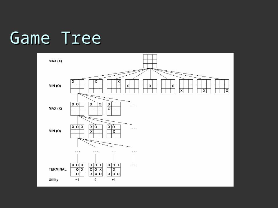
Game TreeGame Tree
37
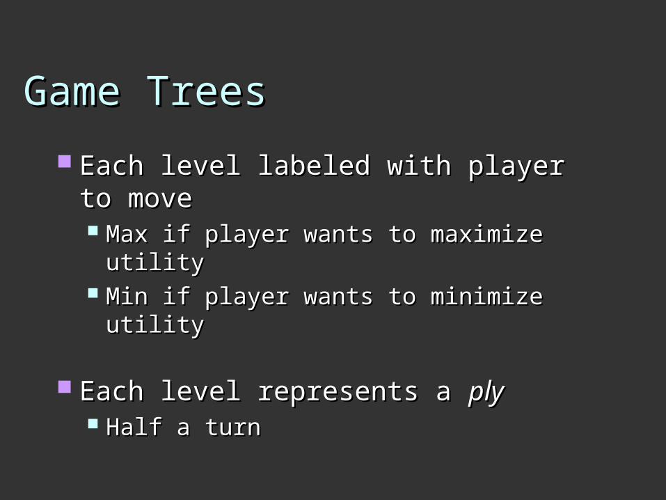
Game TreesGame Trees
Each level labeled with player to Each level labeled with player to movemove Max if player wants to maximize Max if player wants to maximize
utilityutility Min if player wants to minimize utilityMin if player wants to minimize utility
Each level represents a Each level represents a plyply Half a turnHalf a turn
38
Optimal DecisionsOptimal Decisions
MAX wants to maximize utility, but MAX wants to maximize utility, but knows MIN is trying to prevent thatknows MIN is trying to prevent that MAX wants a MAX wants a strategystrategy for maximizing for maximizing
utility assuming MIN will do best to utility assuming MIN will do best to minimize MAX’s utilityminimize MAX’s utility
Consider Consider minimaxminimax valuevalue of each of each nodenode Utility of node assuming players play Utility of node assuming players play
optimallyoptimally

39
Minimax AlgorithmMinimax Algorithm
Calculate minimax value of each Calculate minimax value of each node recursivelynode recursively Depth-first exploration of treeDepth-first exploration of tree
Game tree (aka minimax tree)Game tree (aka minimax tree)
Max node Min node
40
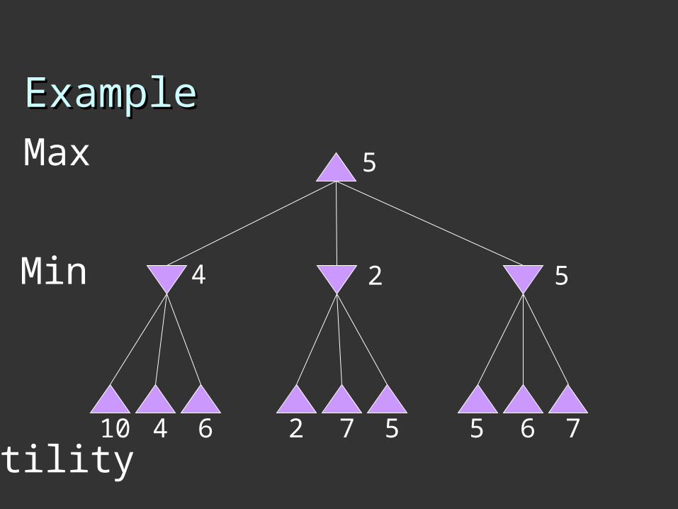
ExampleExample
2 7 5 5 6 710 4 6Utility
Min
Max
4 52
5
41
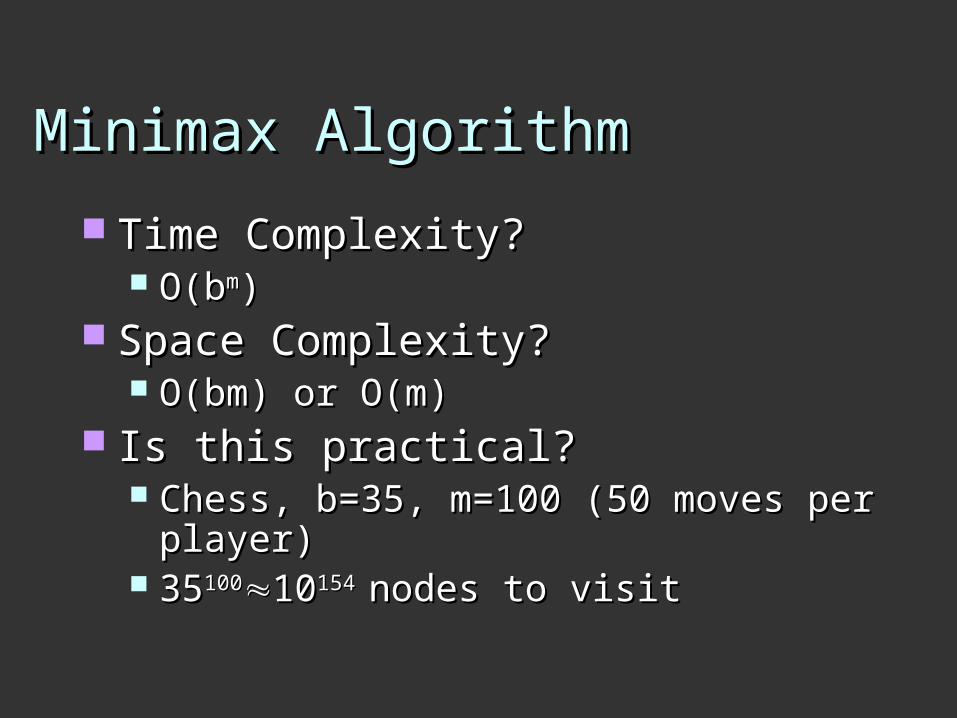
Minimax AlgorithmMinimax Algorithm
Time Complexity?Time Complexity? O(bO(bmm))
Space Complexity?Space Complexity? O(bm) or O(m)O(bm) or O(m)
Is this practical?Is this practical? Chess, b=35, m=100 (50 moves per Chess, b=35, m=100 (50 moves per
player)player) 35351001001010154 154 nodes to visitnodes to visit
42
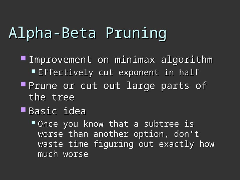
Alpha-Beta PruningAlpha-Beta Pruning
Improvement on minimax algorithmImprovement on minimax algorithm Effectively cut exponent in halfEffectively cut exponent in half
Prune or cut out large parts of the treePrune or cut out large parts of the tree Basic ideaBasic idea
Once you know that a subtree is worse Once you know that a subtree is worse than another option, don’t waste time than another option, don’t waste time figuring out exactly how much worsefiguring out exactly how much worse
43
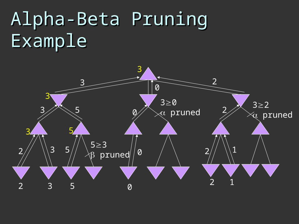
Alpha-Beta Pruning Alpha-Beta Pruning ExampleExample
2 3 5
3
3
02 1
53 pruned2 3 5
3 5
3
0
030 pruned
0
2 1
232 pruned
2
3
5


![Puzzles to Puzzle You [eBook]](https://static.fdocuments.us/doc/165x107/55cf975a550346d0339124fc/puzzles-to-puzzle-you-ebook-pdf.jpg)