Class alliances and conflict: an explanation of political transitions in

nineteenth-century Europe

Sung-Ha Hwanga,∗

aCollege of Business, Korea Institute of Science and Technology (KAIST), Seoul, Korea

Abstract

I develop a model analyzing common interests and conflict among four classes—capitalists,

workers, landlords, and peasants in nineteenth century Europe—and show that strong class

position, based on a high degree of organization and solidarity, may actually be detrimental

to the economic and political advantage of that class. This occurs when a strong class is

excluded from a major class coalition via coalition formation processes. The reason is that

the weak class, if they enjoy bargaining power over even weaker classes within a coalition,

may not want to form a coalition with the strong class. I apply the main results to coalition

formation and political transitions in nineteenth-century European society.

Keywords: Class alliances, conflict, coalition formation, political power, political transition

JEL Classification Numbers: C71, C78, D72

∗April 1, 2017. The research of S.-H. H. was supported by the National Research Foundation of KoreaGrant funded by the Korean Government (NRF-2016S1A5A8019496). I would like to thank to AmitavaDutt, Rajiv Sethi, Gilbert Skillman, Peter Skott, Roberto Veneziani, and participants of the Analytic Po-litical Economy Workshop 2015 at the University of Notre Damme. Special thanks to Samuel Bowles whoencouraged me to work on this project and provided many helpful comments.

Email address: sungha@business.kaist.ac.kr (Sung-Ha Hwang)

1. Introduction

Many social scientists, such as Gerschenkron (1943), Kindleberger (1951), Moore (1965),

Gourevitch (1977), Luebbert (1991), and Stephens et al. (1992), have emphasized the role

of class alliances and conflict or, more generally, coalition formation among various classes

in political and institutional changes in nineteenth-century Europe. According to Moore

(1965), in Germany the Junkers successfully formed an alliance, the so-called solidarity bloc,

with capitalists in big industries and peasants and repressed industrial workers, resulting

in delayed democratization. It is interesting to observe that the industrial working class

in nineteenth-century German society was well-organized and stronger than other classes in

that society:

Although Britain experienced the first industrial revolution and France de-

veloped the first significant socialist associations, Germany produced the largest

and best-organized workers’ movement in the late nineteenth century. By the

mid-1890s, German social democracy had successfully built a mass party and a

centralized trade union movement...(Nolan, 1986, p.352).

Can a coalition excluding a strong class—e.g., the solidarity bloc in nineteenth century

Germany—form as an equilibrium outcome, leading to the political failure of this class?

If so, under which socio-economic conditions is such a coalition stable? To study these

questions, I develop a model of coalition formation among four players who share common

interests and conflict with each other. While the existing literature, by emphasizing the role

of class alliances and conflict, offers a detailed historical description of coalition formation

among classes and its implications for ensuing political transitions, few studies provide a

formal model to explain the process of coalition formation among classes.

1

Economic and political problems have been examined primarily within the context of a

dyadic relationship between two classes. In these models, two classes may only exclusively

have either a common or conflicting interest. However, as the history of coalition formation

in nineteenth-century European countries shows, two classes may have both common and

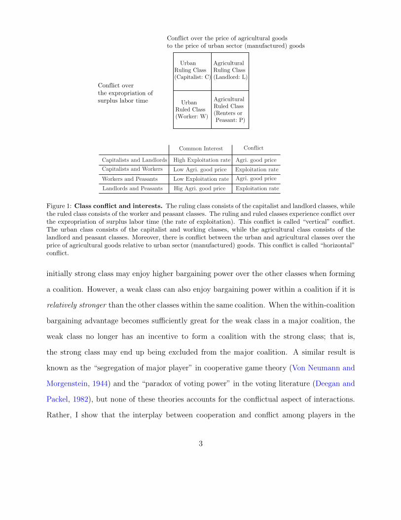
conflicting interests at the same time (see Figure 1; Bowles (1984)). The expropriation of

surplus labor time of wage workers in urban sectors and renters (peasants) in agricultural

sectors is of common interest to the ruling class, namely, capitalists and landlords (vertical

conflict). However, the two ruling classes may experience conflict over the price of an agri-

cultural good relative to the price of an urban sector (manufactured) good, if the two sectors

exchange goods (horizontal conflict). In a similar vein, the working and peasant classes also

have common and conflicting interests over the relative price.

To study these seemingly complicated and intertwined common and conflicting interests,

I develop a four-class coalition model, in which pairs of classes have conflicting interests with

other pairs (pairs in the horizontal rows and vertical columns in Figure 1). By explicitly intro-

ducing a parameter measuring the relative importance of these two kinds of conflicts (vertical

versus horizontal), I study the economic conditions suitable for forming various coalitions.

Specifically, I show that when both vertical and horizontal conflicts are both important, the

exclusion of a politically superior class from the winning coalition might occur. Thus, the

originally strong class can end up being disadvantaged. Though, in general, the initially

more advantaged group is believed to remain more successful economically and politically,

this may not be the case when various common interests and conflict are concurrent.

The main reason for this paradoxical result is as follows. When the four classes form

coalitions, within- and between-coalition bargaining processes occur simultaneously. The

2

Conflict over the price of agricultural goods to the price of urban sector (manufactured) goods

Conflict over the expropriation ofsurplus labor time

UrbanRuling Class(Capitalist: C)

AgriculturalRuling Class(Landlord: L)

Urban Ruled Class(Worker: W)

AgriculturalRuled Class(Renters or Peasant: P)

Capitalists and Landlords

Common Interest Conflict

Capitalists and Workers

Workers and Peasants

Landlords and Peasants

High Exploitation rate

Low Agri. good price

Low Exploitation rate

Hig Agri. good price

Agri. good price

Exploitation rate

Agri. good price

Exploitation rate

Figure 1: Class conflict and interests. The ruling class consists of the capitalist and landlord classes, whilethe ruled class consists of the worker and peasant classes. The ruling and ruled classes experience conflict overthe expropriation of surplus labor time (the rate of exploitation). This conflict is called “vertical” conflict.The urban class consists of the capitalist and working classes, while the agricultural class consists of thelandlord and peasant classes. Moreover, there is conflict between the urban and agricultural classes over theprice of agricultural goods relative to urban sector (manufactured) goods. This conflict is called “horizontal”conflict.

initially strong class may enjoy higher bargaining power over the other classes when forming

a coalition. However, a weak class can also enjoy bargaining power within a coalition if it is

relatively stronger than the other classes within the same coalition. When the within-coalition

bargaining advantage becomes sufficiently great for the weak class in a major coalition, the

weak class no longer has an incentive to form a coalition with the strong class; that is,

the strong class may end up being excluded from the major coalition. A similar result is

known as the “segregation of major player” in cooperative game theory (Von Neumann and

Morgenstein, 1944) and the “paradox of voting power” in the voting literature (Deegan and

Packel, 1982), but none of these theories accounts for the conflictual aspect of interactions.

Rather, I show that the interplay between cooperation and conflict among players in the

3

formation of coalitions yields this paradox (see Section 2 for related discussion).

I also review the historical evidence of coalition formation in nineteenth-century Germany

and England and argue that the historical formation of coalitions agrees with the predictions

of the model. Provided that the solidarity bloc in Germany is anti-democratic, the model’s

result also suggests a possible link between trade policy and democracy through coalition

formation, which is the central theme of Geschenkron’s Bread and Democracy (Gerschenkron,

1943). Section 2 reviews the related literature and Section 3 proposes a formal model. Section

4 explains a method of finding equilibrium coalition structures and Section 5 presents the

main results. Historical applications follow in Section 6. Section 7 concludes the paper.

2. Related Literature

In this section, I review the existing literature on coalition formation and explain the

relationship between my approaches and the existing literature. There exists theoretical

analysis of endogenous class formation and alliances from the political economy perspective.

Bowles (1984) studies how economic relations among various classes can give rise to class

alliances and conflict as follows:

Similarly, if renters [of the land; farmers] exchange some of their r-good [an

agricultural good] income for c goods [a manufactured good], they have a com-

mon interest with landlords in the relative price of r-goods. Not surprisingly,

when tariff debates have dominated political discourse and organization, as in

Germany before World War I, renter-landlord alliances have been common... On

the other hand, workers and renters share a common interest in reducing the rent

share or in raising s [the wage worker premium]...Thus, where the vertical issues

4

of redistribution in a class relationship become politically salient, renter-worker

alliances are more likely to develop (p. 113, Bowles 1984).

He develops the income distribution model consisting of four classes (renters, landlords, wage

workers, and capitalists) and identifies the economic conditions for class conflict and alliances

among these four classes.

Roemer also studies the problem of endogenous class formation in various contexts. In

Roemer (1982), he considers four classes consisting of (i) those who must hire labor power

to optimize, (ii) those with some capital, but must sell labor power to optimize, (iii) those

who can optimize without hiring or selling labor power, and (iv) those with no capital and

must sell labor power. He demonstrates that society is endogenously partitioned into four

classes and proves the class exploitation correspondence principle in which society is, in

turn, partitioned into exploited and exploiter. In Roemer (1985), he also studies revolution

by combining a non-cooperative game with a cooperative game framework and shows that

the ideological aspects of the revolutionist and dictator arise from the optimizing behaviors.

Roemer emphasizes the role of leaders in forming a coalition among the masses. Particularly,

he shows that when a coalition is poor-connected (i.e. the coalition contains all agents

whose income is less than a threshold level of income), the revolutionist optimal strategy is

progressive redistribution. Finally, Roemer (2001) presents a four class model of workers, the

middle class, the landed peasantry and the agricultural proletariat to test Luebbert’s theory

of regime choice in European countries during the interwar period and provides strong support

for it.

Roemer’s studies focus on the role of leaders or parties in inducing the endogenous for-

mation of class or coalition formations, while my approaches emphasize the role of common

5

interests and conflict among the four classes. My work is thus more in line with Bowles

(1984) in that I consider the same four classes and similar class common interests and con-

flict. However, I further study the endogenous formation of coalitions among the four classes

and explore the political implications of such coalition formations.

There are also two main modeling approaches in coalitional formation games: (i) coop-

erative approaches and (ii) non-cooperative approaches. I will briefly review the two kinds

focusing on a weak player’s advantage, or equivalently, a strong player’s disadvantage in

which a player of a game with high bargaining power may come to be excluded from the

coalition (refer to the survey of coalition formation by Ray and Vohra (2015)).

First, there is an abundant literature of cooperative game theory devoted to coalition

formation. The result of weak players’ advantage is first discussed in Von Neumann and

Morgenstein (1944) in Section 55, where they study “an apex game”–a variant of a voting

game in which one major player along with any single minor player can form a winning

coalition, or all minor players without the major player can form a winning coalition. Hart

and Kurz (1984) show that the coalition of all minor players excluding the major player can

be a stable coalition under some conditions.

Specifically, they introduce two notions of stability—one based on the assumption that

a coalition abandoned by some of its members breaks apart into singletons (called the “fall

apart” scenario and the γ-model; see Definition 2 for a more precise definition) and another

based on the assumption that the remaining players from the coalition abandoned by one

player still form a coalition (called the “stick together” scenario and the δ-model; see Def-

inition 2 again). They show that when the total number of players (n) is greater than 5,

the coalition of minor players excluding the major player is stable under the γ- model, while

6

this is not the case under the δ-model. This is because the minor players, each obtaining

payoffs 1/(n − 1) in the winning coalition (because of equal division of the surplus of 1)

cannot improve their payoffs by leaving the minor coalition under the γ-model. If one minor

player defects from the minor players’ coalition, according to the γ-stable scenario, all the

other minor players end up standing alone, which deteriorates the bargaining position of the

defecting minor player in the new winning coalition with the major player. Hence, defection

from the minor coalition does not improve the payoff. However, under the δ-stable scenario,

exclusion of the major player (the apex player) cannot occur since any minor player can

form a deviation coalition with the major player obtaining 1/2. This is because, under the

δ-model, all the deserted minor players still remain as a coalition; based on this, the defect-

ing player can enjoy bargaining power within the winning coalition with the major player,

obtaining 1/2.

Also, from the framework of cooperative solutions, various indices relating voting rights

(or voting weights) to voting power were developed. (the Shapley and Shubik index (Shapley

and Shubik, 1954) and the Banzhaf power index). This literature also reports the so-called

“the paradox of the voting power”(Van Deemen and Rusinowska, 2003). There are several

different paradoxes—one of them is called the paradox of redistribution. This refers to the

situation in which a player gains in terms of voting weights, but loses in voting power. Fischer

and Schotter (1978) show that the paradox can occur for the Banzhaf index when n ≥ 6 and

for the Shapley-Shubik index when n ≥ 7. These are related to the weak player’s disadvantage

in the sense that a weak voter with lower voting weight may gain, but the paradox arises

because of the computation methods of indices, neither from class interactions nor from the

endogenous formation of coalitions associated with them.

7

Another important strand in the literature on coalition formation and bargaining is based

on non-cooperative game approaches initiated by the celebrated work of Baron and Ferejohn

(1989). They show that “the continuation values of all parties [in the government formation

game] can be equal even though the recognition probabilities are unequal.”(p.1194) This is

because the two largest parties prefer to form a government with the smallest party, since

the smallest party expects a lower continuation value (out of equilibrium). In a similar

vein, Eraslan and McLenna (2013) write “the overall tendency should be in the direction

of more expensive coalitions being chosen less frequently by proposers” (p.2197). Thus, the

weak players’ advantages in this context are related to the power of a proposal, or so-called

“formatuer advantages” (Ansolabehere et al., 2005). Snyder et al. (2005) also show that in a

corner equilibrium of their legislative bargaining model, players with voting weights less than

a certain threshold have expected payoffs greater than their shares of the total voting weights

(p.983). This is again related to the proposal power, but in this case the proposal advantages

of the weak player himself in that the weak player—so weak that no other proposers ever

choose him as a coalition partner—can expect a greater expected payoff just because of the

proposal power.

In sum, the existing literature shows weak players’ advantages in a cooperative game

framework when exclusion of the major player in a winning coalition can occur under some

conditions. However, this is sensitive to the assumption for the coalition formation processes

(i.e., γ-model or δ-model). In a noncooperative game framework, weak players’ advantages

may obtain when large parties, as proposers, would like to form a coalition with the weak

player or when the weak player himself has proposal power.

In contrast to the existing literature, my main results derive from the aspect of class

8

interests and among four players, pairs of two players having common interests and con-

flict with other pairs. My approach also explicitly accounts for within-group bargaining and

between-group bargaining among four classes. Specifically, I use coalitional values, which

generalize the Shapley value—one of the most frequently used solution concepts—to the con-

text of coalition formation. My method and analysis thus belong to the class of cooperative

bargaining literature, but differ from it in that the conflicting interests (see Figure 1), rather

than the cooperative features, drive the main results for the weak players’ advantages. I also

consider the coalition structure, i.e., a partition of a set of players, which allows study of

the interactions within- and between-group bargaining processes simultaneously—an aspect

absent in the existing non-cooperative bargaining literature.

As a result, Proposition 2 (i), shows that when Player W in Figure 1 is strongest, the

opposing coalition {CLP} is stable under both the γ- and δ-models. The main reason is that

the weak C and P players, having simultaneous common and conflicting interests with W ,

can enjoy bargaining power over even the weaker class L through within bargaining processes,

since L has only conflict but no common interest with W .

3. Model

When two different categories of groups are considered, subgroups within these groups

may have both common interests and conflict. For example, the divisions of a society into

ruling versus ruled classes and into urban versus rural populations give rise to four subgroups

(Figure 1): the urban ruling class (capitalists), agricultural ruling class (landlords), urban

ruled class (workers), and agricultural ruled class (peasants). These four classes have relation-

ships, such that each has both common and conflicting interests with another, as explained in

9

1A

2A

1B

: ( 1, 1)C A B : ( 1, 2)L A B

: ( 2, 1)W A B : ( 2, 2)P A B

2B

Figure 2: Preferences of Players C,L,W, and P . Players C and L prefer A1 to A2, while players W and Pprefer A2 to A1 (vertical conflict). Also, players C and W prefer B1 to B2, while players L and P prefer B2to B1 (horizontal conflict).

the Introduction. Another example includes the following two categories of groups: political

party membership and gender. Consider the categories of female versus male and Republi-

cans versus Democrats; a female Republican may share similar political opinions with a male

Republican, but they may conflict on gender issues. Similarly, a female Republican may

have common interests in gender issues with a female Democrat, but may have conflicting

views on political agendas (see also Lee and Roemer, 2006, for race vs political orientation

categories).

To study these four-way interactions, I suppose that four players (denoted by C, L,

W, and P ) have common interests and conflict over two kinds of policies (denoted by A

and B). Policy A can be either A1 or A2, and policy B can also be either B1 and B2;

thus there are in total four possible outcomes: (A1, B1), (A1, B2), (A2, B1), and (A2, B2)

(see Figure 2). Thus, players have vertical conflict over policy A and horizontal conflict

over policy B. As an example, sourced again from the Introduction, policy A is the rate

of exploitation e, with A1 and A2 representing the high rate (eH) and low rate (eL) of

exploitation, respectively. Similarly, policy B is the price of an agricultural good (τ) relative

to the price of a manufactured good (from the urban sector), with τL and τH being the low

and high relative prices (thus B1 and B2), respectively.

Denoting Ai � Aj when Ai is preferred to Aj, suppose that

10

• player C : A1 � A2 and B1 � B2 (i.e, eH � eL and τL � τH).

• player L : A1 � A2 and B2 � B1 (i.e, eH � eL and τH � τL).

• player W : A2 � A1 and B1 � B2 (i.e, eL � eH and τL � τH).

• player P : A2 � A1 and B2 � B1 (i.e, eL � eH and τH � τL).

To obtain a simple payoff representation of the above preference relations, I assign a payoff

1/2 to the more preferred outcome and a payoff −1/2 to the less preferred outcome, and

I assume that the payoff from an outcome of two policies is the sum of the payoffs from

each policy. For example, player C obtains payoff 1 from (A1, B1) (i.e., 1 = 1/2 + 1/2),

payoff 0 from (A1, B2) and (A2, B1) (0 = 1/2 + (−1/2)), and payoff −1 from (A2, B2)

(−1 = −1/2 + (−1/2)). In this way, the following matrix shows the payoff representations

of the above preference relations of each player:

(A1, B1) (A1, B2) (A2, B1) (A2, B2)C 1 0 0 -1L 0 1 -1 0W 0 -1 1 0P -1 0 0 1

(1)

In general, the relative importance of vertical conflict (about A) and horizontal conflict

(about B) varies from situation to situation. For example, dramatic changes in trade envi-

ronments due to a sudden inflow of cheap agricultural products from outside may escalate

the horizontal conflict between the urban and agricultural sectors. To study these situations,

I introduce a (slightly) more flexible specification of payoffs than (1):

(A1, B1) (A1, B2) (A2, B1) (A2, B2)C 1 κ −κ −1L κ 1 −1 −κW -κ −1 1 κP -1 −κ κ 1

(2)

11

Conflict over τ Conflict over τ

0κ = 1κ =1κ = −

Con

flic

t ov

er e

Con

flic

t ov

er e

UrbanRuling Class (C)

AgriculturalRuling Class (L)

UrbanRuled Class (W)

AgriculturalRuled Class (P)

UrbanRuling Class (C)

AgriculturalRuling Class (L)

UrbanRuled Class (W)

AgriculturalRuled Class (P)

UrbanRuling Class (C)

AgriculturalRuling Class (L)

UrbanRuled Class (W)

AgriculturalRuled Class (P)

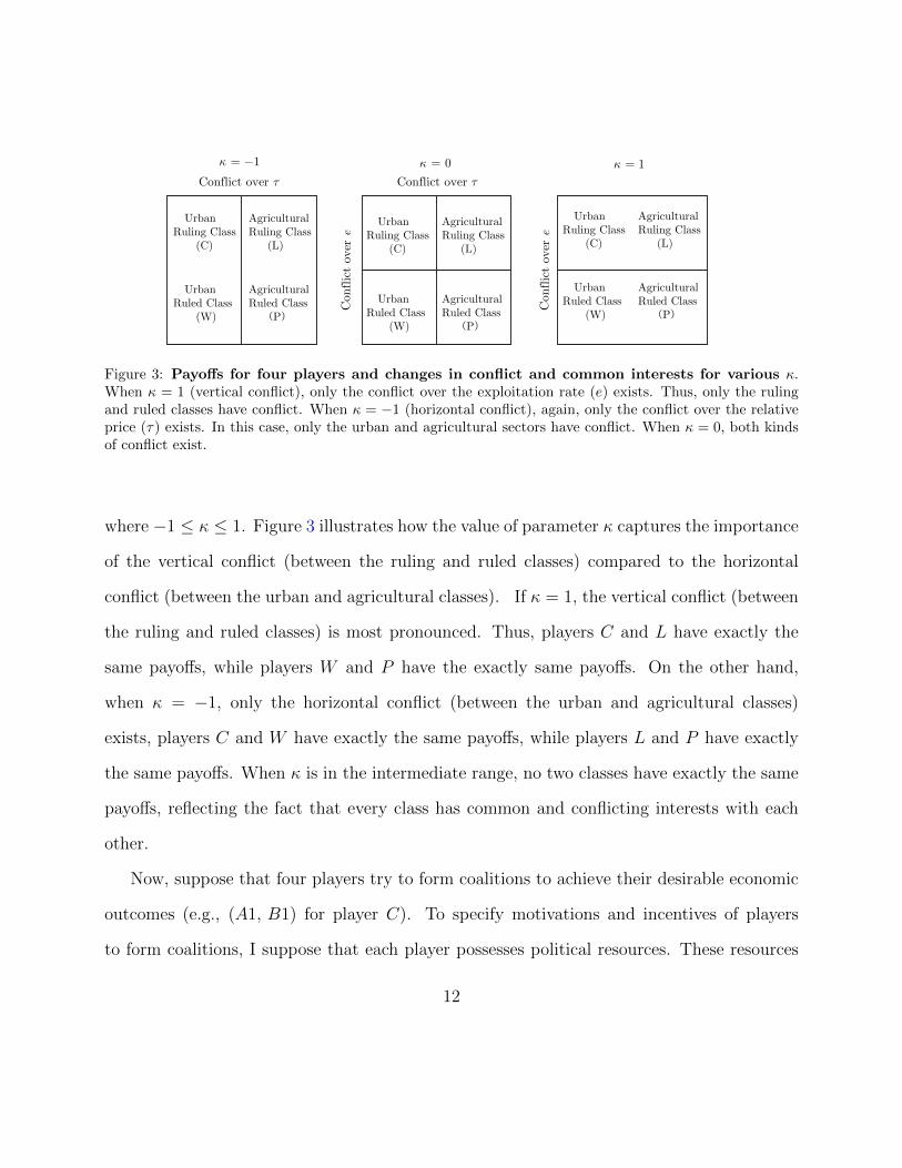
Figure 3: Payoffs for four players and changes in conflict and common interests for various κ.When κ = 1 (vertical conflict), only the conflict over the exploitation rate (e) exists. Thus, only the rulingand ruled classes have conflict. When κ = −1 (horizontal conflict), again, only the conflict over the relativeprice (τ) exists. In this case, only the urban and agricultural sectors have conflict. When κ = 0, both kindsof conflict exist.

where −1 ≤ κ ≤ 1. Figure 3 illustrates how the value of parameter κ captures the importance

of the vertical conflict (between the ruling and ruled classes) compared to the horizontal

conflict (between the urban and agricultural classes). If κ = 1, the vertical conflict (between

the ruling and ruled classes) is most pronounced. Thus, players C and L have exactly the

same payoffs, while players W and P have the exactly same payoffs. On the other hand,

when κ = −1, only the horizontal conflict (between the urban and agricultural classes)

exists, players C and W have exactly the same payoffs, while players L and P have exactly

the same payoffs. When κ is in the intermediate range, no two classes have exactly the same

payoffs, reflecting the fact that every class has common and conflicting interests with each

other.

Now, suppose that four players try to form coalitions to achieve their desirable economic

outcomes (e.g., (A1, B1) for player C). To specify motivations and incentives of players

to form coalitions, I suppose that each player possesses political resources. These resources

12

can be used to form a winning coalition, which can set the policy (A,B) for the society.

To represent these resource constraints, let each player possess a certain proportion of total

resources, with αi being the proportion of player i’s political resources, where αi ∈ [0, 1],

and∑αi = 1. That is, αC , αL, αW , and αP are the proportions of political resources for

players C, L, W , and P , respectively. This introduction of political resources resembles the

distinction between de jure political power and de facto political power in Acemoglu et al.

(2005).

Here de jure political power refers to power that originates from the political

institutions in society...There is more to political power than political institutions,

however. A group of individuals, even if they are not allocated power by political

institutions, for example as specified in the constitution, may nonetheless possess

political power. Namely, they can revolt, use arms, hire mercenaries, co-opt

the military...We refer to this type of political power as de facto political power

(Acemoglu et al., 2005, p.4).

Even though the working class (W ) and the peasant class (P ) do not have de jure political

power, they may have de facto political power. When classes form a coalition, they use their

de facto political power to achieve a goal.

The worth of coalition S, v(S), is defined as the amount of payoffs the coalition can

achieve. To define this more precisely, first call coalition S winning if the aggregate political

resources of the coalition is greater than a certain number, α, where α ∈ [1/2, 1]. Thus, S

becomes a winning coalition if∑

i∈S αi ≥ α. If a coalition becomes a winning coalition, this

coalition can choose one of policies (among (A1, B1), (A1, B2), (A2, B1), and (A2, B2)) as

a policy at the society’s level. The winning coalition is assumed to choose the proposal that

13

maximizes the sum of payoffs of the coalition members: max(A,B)

∑i∈S πi(A,B). However, S may

not be a winning coalition. In this case, the players outside S may or may not form a winning

coalition, and thus, members in S are uncertain about which policy would be adopted. Since

the worth of the coalition, v(S), is the expected payoffs to members when joining S, I assume

that members of non-winning coalitions expect that any of four policies is equally likely and

use the expected value of the payoffs as a worth of this coalition1: i.e.,

E[πi(A,B)] = πi(A1, B1)1

4+ πi(A1, B2)

1

4+ πi(A2, B1)

1

4+ πi(A2, B2)

1

4= 0.

This discussion leads to the following definition of the worth of coalition S:

v(S) =

max(A,B)

∑i∈S πi(A,B) if

∑i∈S αi ≥ α∑

i∈S E[πi(A,B)] if∑

i∈S αi < α

(3)

Note that∑

i∈S E[πi(A,B)] = 0 since E[πi(A,B)] = 0 for all i.

The specification of the worth completes the presentation of the underlying model. The

next step is to find stable coalition structures, and this involves three steps (see Hart and

Kurz (1983)): 1) find the coalition structure values, 2) derive the coalition formation game,

and 3) identify the stable coalition structures.

1Players outside S may form a winning coalition, which affects the payoffs of players in S. This kind ofexternality is a key component to the analysis that follows, and the coalition structure value for a coalition,defined in Section 4, accounts precisely for this externality.

14

4. Method

4.1. Coalition structure values (CS-values)

A coalition structure B is a finite partition B = {B1, B2, ..., Bm} of the set of all players

N ; i.e.,⋃mk=1Bk = N and Bk

⋂Bl = ∅ for all k, l ∈ M = {1, ....m}, k 6= l. I write

coalition structure B = [B1|B2| · · · |Bm]. For example, coalition structure [CL|WP ] consists

of a coalition {C,L} and another coalition {W,P}.

Definition 1 (Owen, 1977). For each coalition structure B, a coalition structure value (or

CS-value) for each player i ∈ N is defined as :

φi(v,B) =∑H⊂Mj/∈H

∑S⊂Bj

i/∈S

h!(m− h− 1)!s!(bj − s− 1)!

m!bj![v(Q ∪ S ∪ i)− v(Q ∪ S)] (4)

for Bj ∈ B and i ∈ Bj where h, s and bj are the cardinalities of H, S and Bj, and Q =⋃k∈H Bk, M = {1, ....m} such that B = {B1, B2, ..., Bm}.

The “value” corresponds to the evaluation by the players given the coalitional structure.

The value summarizes the complex possibilities facing each player in coalition formation

games (Roth, 1988, p.4). Using the values attached to each coalition structure, players are

able to compare their “prospects” in the various coalition structures and decide whether to

change their coalitions. There is an alternative way of computing values differently from (4),

namely, Aumann–Dreze value (Aumann and Dreze, 1974). In the Aumann–Dreze value, the

interactions between coalitions are absent, and thus, between-group bargaining processes are

neglected. Since I wish to study the interactions of the within- and between-group bargaining

processes under various coalition structures, I adopt the CS-values in (4) for analysis.

15

4.2. Coalition formation games

In the second step, I specify a coalition formation game, in which a player’s strategies are

the choices of coalitions to which the player wishes to belong. For example, the strategies

of player C are given by {C}, {C,L}, {C,W}, {C,P}, {C,L,W}, {C,L, P}, {C,W,P},

and {C,L,W, P}. The coalitional payoffs for players are based on the CS-values, computed

in the previous step. However, to define coalitional payoffs, one has to specify how each

player’s choices of strategies determine a coalition structure. For example, consider a coali-

tion structure [C|LWP ], which indicates the formation of coalition {L,W,P}. If L leaves her

coalition, her previous coalition can either fall apart or stick together. So, the resulting coali-

tion structure following L’s departure would be either [C|L|W |P ] or [C|L|WP ] depending

on the interpretation of coalitions. The first case—the “fall apart” scenario—is based on the

view that a coalition results from a unanimous agreement, and model γ below describes this

type of coalition formation. The second case—the “stick together” scenario—corresponds to

a situation, in which in a large coalition, a small number of players leaving the coalition do

not influence the other coalition members’ agreement to act together. This case is specified

by model δ:

Definition 2 (Hart and Kurz, 1983). There are two coalition formation games:

Model γ : The game Γv,N is defined as follows:

(M1) The set of players is N.

(M2) For each i ∈ N , the set of player i’s strategy Σi consists of all coalitions S that contain

i, namely, Σi = {S ⊂ N |i ∈ S}.

(M3) For each n-tuple of strategies σ = (S1, S2, ..., Sn) ∈ Σ1×Σ2× ...×Σn , where n = |N |

16

and each i ∈ N , the payoff to i is φi(v,B(γ)σ ), where

T iσ =

Si, if Sj = Si for all j∈ Si

{i}, otherwise

and B(γ)σ = {T iσ|i ∈ N}.

Model δ: The game ∆v,N is given by (M1), (M2), and (M4) :

(M4) For each n-tuple of strategies σ = (S1, S2, ..., Sn) ∈ Σ1×Σ2× ...×Σn and each i ∈ N ,

the payoff to i is φi(v,B(δ)σ ), where

B(δ)σ = {T ⊂ N |i, j ∈ T if and only if Si = Sj}.

4.3. Stable coalition structures

After specifying the coalition formation game, the stable coalition structures need to

be identified in the final step. As a stable coalition structure is defined as an equilibrium

outcome, a proper equilibrium concept addressing coalitional deviations is needed. For this

purpose, I rely on the concept of strong equilibrium, first defined by Aumann (1967) and

subsequently adopted by Hart and Kurz (1983). According to this concept, a stable coalition

structure is defined as a coalition structure where no defection by any subgroup of players or

an individual player is desirable.

Definition 3 (Hart and Kurz, 1983). The coalition structure B is γ-stable (or δ-stable) in

the game (v,N) if σB is a strong equilibrium in Γv,N(or ∆v,N); i.e., if there exists no nonempty

T ⊂ N and no σi ∈ Σi for all i ∈ T , such that φi(v, B) > φi(v,B) for all i ∈ T , where B

corresponds to((σi)i∈T , (σ

jB)j∈N\T

)by (M3) (or (M4))

17

5. What are stable coalitions?

In the analysis to follow, I focus on the case where one player’s political power is not so

great that (i) only a single player cannot win by standing alone (hence, αi < α) and (ii) any

of three players can form a winning coalition (i.e., 1− αi > α):

αi < α, 1− αi > α for all i ∈ {C,L,W, P} (5)

In Panel A Figure 4, I present the region in which parameters, αW , αC , αL, satisfy the condi-

tions in (5) when αP = 0.25. The triangle in Panel A Figure 4 thus corresponds to the set of

∆ := {(αW , αC , αL) : αW+αC+αL = 0.75, αi ≥ 0 for all i} (recall that αC+αL+αW+αP = 1

and α = 0.25), where each point in the triangle uniquely corresponds to a point in ∆. For

example, point a, point b and point c correspond to (αW , αC , αL) = (0.75, 0, 0), (0, 0.75, 0),

and (0, 0, 0.75), respectively (see the caption in Figure 1 for more details). The dark shaded

region in Panel A shows the set of parameters, αW , αC , and αL, satisfying conditions in (5).

First, consider the case where only vertical conflict exists between players C and L (the

ruling class) versus players W and P (the ruled class) exists; i.e., κ = 1. In this case, policy

A (the exploitation rate, e) is the only factor determining economic interests of four players.

Thus, it is plausible to expect that the stable coalition structure is given by [CL|WP ]. This

is indeed the case when the sum of political resources of players C and L is greater than α

so that players C and L can form a winning coalition, while the sum of political resources

of players W and P is insufficient to form a winning coalition (see the dark shaded region in

Panel B Figure 4). A similar observation is possible for the antipodal case, κ = −1, when

players C and W can form a winning coalition while players L and P cannot.

18

Panel A Panel B Panel C

0.75Cα = 0.75Lα =

0.75Wα =

a

b c

d

e f

g h

i j

0.75Wα =

0.75Cα = 0.75Lα =

g h

i j

e f

g

i

0.75Wα =

0.75Cα = 0.75Lα =

Figure 4: Regions satisfying political power conditions in (5), Proposition 1 (i) and Proposition1 (ii) when α = 1/2 and αP = 0.25. The simplex shows the set of all parameters, αW , αC , and αL in theset of ∆ := {(αW , αC , αL) : αW +αC +αL = 0.75, αi ≥ 0 for all i} (recall that αC +αL +αW +αP = 1 andαP = 0.25). Points a, b, c, d, e, f , g, h i and j correspond to parameters, (αW , αC , αL) : a = (0.75, 0, 0),b = (0, 0.75, 0), c = (0, 0, 0.75), d = (0.25, 0.25, 0.25) e = (0.5, 0.25, 0), f = (0.5, 0, 0.25), g = (0.25, 0.5, 0), h =(0.25, 0, 0.5), i = (0, 0.5, 0.25), j = (0, 0.25, 0.5), respectively. The dark shaded region in Panel A shows therange of parameters satisfying conditions in (5), and the dark shaded regions in Panels B and C show theranges of parameters satisfying conditions in Proposition 1 (i) and (ii), respectively. Note that the dark shadedregions are located adjacent to the edge connecting αC and αL (the classes with more political resources inProposition 1 (i)) in Panel B and the edge connecting αC and αW (the classes with more political resourcesProposition 1 (ii)) in Panel C

Proposition 1. Suppose that the assumptions in (5) hold. Then the following results hold:

(i) If κ = 1, αC + αL > α > αW + αP , then [CL|WP ] is γ− and δ−stable.

(ii) If κ = −1, αC + αW > α > αL + αP , then [CW |LP ] is γ−and δ−stable.

Proof. See the Appendix.

Next, consider the case where both vertical and horizontal conflicts are present. For

expositional purpose, suppose that αC = αL = αP . The first case is the situation where

the political power of player W is the strongest: αC = αL = αP < αW < α. For example,

(αC , αL, αW , αP ) = (0.23, 0.23, 0. 31, 0.23) for α = 0.5. (Recall the assumptions of αC =

αL = αP and αC + αL + αW + αP = 1.) In this case, only player W is powerful enough to

form winning coalitions of size two. All the other players need either player W or two more

19

other players to form a winning coalition. Precisely, the winning coalitions are {CW},{LW},

{WP}, {CLW}, {CLP}, {LWP}, {CWP}, and {CWLP} since αi+αj < α for all i, j 6= W ,

αi+αW > α for all i 6= W , and αi+αj+αk > α for all i, j, k. Thus, all the coalitions including

player W are winning coalitions. From the payoff matrix (2), the worth of coalitions, (3), is

given by

v(S) =

1 + κ S = {WP}

1− κ S = {CW}

1 S = {CLW}, {CLP}, {LWP}, {CWP}

0 otherwise

(6)

This game is similar to the so-called apex games in the literature except that v(LW ) = 0

and v(CLWP ) = 0 (Hart and Kurz, 1984). However, these differences turn out to be crucial.

First, since players L and W do not have any common interest (v(LW ) = 0), this introduces

asymmetry among the four players. Second, since there exist two kinds of conflicts among

the four players simultaneously, the grand coalition {CLWP} cannot produce anything,

regardless of policy outcomes. Thus, the underlying game is not super-additive. These two

distinct features, accounting for the conflicting aspects of the four players, introduce different

mechanisms of coalition formation.

To explain how to find coalitional values, suppose that κ = 0 for the simplicity of ex-

position (see the complete CS-values in Table A.3 in Appendix A). I first review how to

compute the Shapley values, because the CS-values for [C|L|W |P ] are, by definition (4), the

same as the Shapley values: (0, -1/6, 1/6, 0). These numbers mean that when the coali-

tion structure is [C|L|W |P ], C, L, W , and P expect 0, -1/6, 1/6, and 0 as their coalitional

20

payoffs, respectively. To understand these numbers, imagine that the players enter a room

in random order, and they are allowed to form a coalition inside the room. First consider

the case where C enters a room. Then, C can be a “positive” pivot player — a player who

contributes a positive worth (+1) as she enters the room (or joins the existing coalition) —

or a “negative” pivot player — a player who contributes a negative worth (−1).

Player C is a positive pivot player when the order of entering is {WCPL}, {WCLP},

{LWCP}, {WLCP}, {PLCW}, {LPCW} (for example, since v(WC) − v(W ) = 1 for

{WCPL}). Thus, C will expect 1/4 by being a positive pivot player, since out of the total

possibilities (4!), the number of orders where C becomes a positive pivot player is 6, thus

contributing a net surplus of +1. On the other hand, when the sequence of entering is

{PWLC}, {WPLC}, {LPWC}, {PLWC}, {WLPC}, {LWPC}, C becomes a negative

pivot player, who contributes a net surplus of −1. This is because when C joins the existing

coalition, its worth drops from 1 to 0. Since C can be a negative pivot player with the

probability of 1/4 (again, = 6/4!), C expects -1/4 from being a negative pivot. As the

expected payoff from the positive pivot and negative pivot are 1/4 and -1/4, respectively,

player C expects 0 payoff on average when the coalition structure is [C|L|W |P ]. A similar

explanation can be applied to the payoff of P , which is also 0.

The Shapley values for players W and L can be verified similarly. Note that W can form

a winning coalition of size two with any other players and player W thus expects the highest

payoff (1/6) under coalition structure [C|L|W |P ]. Also, L can form a winning coalition of

size two only with the more powerful player, W , but L does not have a common interest

with W (v(LW ) = 0). This is why L expects the lowest payoff (−1/6) under the coalition

structure [C|L|W |P ].

21

Between-group bargaining: {C,W}=A, {L}, {P}•

a new worth of coalition {C,W}: 2/3⇒

Sh({L})= -1/3⇒

Sh({P})= -1/3⇒

Sh({CW})= 2/3⇒

Within-group {C,W} bagaining: how to divide 2/3•

Fallback payoffs for C, W: Sh(C), Sh(W) when {C},{L},{W},{P} are players.

⇒

⇒ * * *New worths: (C)=Sh(C)=0, (W)=Sh(W)=1/6, (C,W)=2/3v v v

Shapley values for this new game⇒

⇒

⇒

CS-values for [CW|L|P]

CS(L)=-1/3

CS(P)=-1/3

CS(C)=1/4

CS(W)=5/12

*Sh ({C})= 1/4*Sh ({W})= 5/12

Figure 5: Computations of CS-values. Here Sh( ) is the Shapley value, and CS( ) is the CS-value.

Next, I explain how to compute the CS-values in general(see Figures 5 and 6). Take

the example of [CW |L|P ]; The CS-values are given by (C,L,W, P ) = (1/4, -1/3, 5/12, -

1/3 ) in this case. Figure 5 illustrates the computation of the CS-values for [CW |L|P ],

showing how the CS-values can characterize interactions between and within coalitions. First,

under coalition structure [CW |L|P ], suppose that {CW} forms one representative player A,

and players A, L, and P engage in bargaining (the between-group bargaining step). From

(6) I find the worth function for this new bargaining: v(A) = v(AL) = v(AP ) = 1, and

v(L) = v(P ) = v(LP ) = v(ALP ) = 0. Again, by using the same argument as above, I find

the Shapley values for this new game: (A,L, P ) = ({C,W}, L, P ) = (2/3,−1/3,−1/3). This

is the bargaining process among the coalitions (see “Between-group bargaining” in Figure 5).

Secondly, within-coalition bargaining occurs. Since there is only one coalition, {CW},

consider the bargaining within {CW} only. To determine the bargaining within {CW},

22

I need to identify “disagreement point.” Because the player has an option to leave the

coalition, the natural disagreement point would be the payoff the player expects when she

leaves the coalition. If C or W leaves {CW}, then the resulting coalition structure will be

[C|W |LP ]. Since [C|L|W |P ] = (0,−1/6, 1/6, 0), C has 0 as her “fallback” payoff, and W

has 1/6 as her “fallback” payoff. Using this information, I obtain a new worth function

which occurs within the coalition {CW}: v∗(C) = 0, v∗(W ) = 1/6, and v∗(CW ) = 2/3

(since v∗(A) = 2/3 and (A,L, P ) = (2/3,−1/3,−1/3) from the between-coalition bargaining

processes). Again, I find the Shapley values for this case, and they are (C,W ) = (1/4, 5/12).

Combining the between- and within-coalition bargaining steps, I find the CS-values [CW |L|P ]

are (C,L,W, P ) = (1/4,−1/3, 5/12,−1/3). The CS-values for [CLP |W ], where player W is

excluded from the winning coalition {CLP}, can be similarly found (see Figure 6).

By comparing CS-values for [CW |L|P ], (C,L,W, P ) = (1/4, -1/3, 5/12, -1/3 ) and CS-

values for [CLP |W ], (C,L,W, P ) = (1/4, 0, -1/2, 1/4 ), it is easy to see that C cannot obtain

a positive payoff by deviating from [CLP |W ] to [CW |L|P ]. Intuitively, player C contributes

to coalition {CLP} as much as she contributes to coalition {CW}, since C in {CLP} plays a

relatively important role compared to L. Even though coalition{CW} coalition may enjoy a

higher bargaining power via between-coalition bargaining processes because of the presence of

the strong player, W (e.g., {CW} versus {L}, {P}), the advantage for C via within-coalition

barga0ining in {CLP} is the same as that from between-coalition bargaining. That is, the

CS-values for C are 1/4 for both [CLP |W ] and [CW |LP ]. Thus, C does not have an incentive

to defect from coalition {CLP}. This shows that C enjoys bargaining power over an even

weaker player (L) within the coalition {CLP}. The similar observation holds for player P .

Also, L cannot obtain a better payoff by deserting either C or P and making a coalition with

23

Between-group bargaining: {C, L, P}, {W}•

a new worth of coalition {CLP}: 1/2⇒

Sh({W})=-1/2⇒

Sh({CLP})= 1/2⇒

Within-group {CLP} bagaining: how to divide 1/2•

Fallback payoffs for C, L, P: Sh(C)=0, Sh(L)=-1/6, Sh(P)=0 when {C},{L},{W},{P} are players.

⇒

⇒

Shapley values for this new game⇒

CS-values for [CLP|W]

CS(W)=-1/2

Fallback payoffs for CL: Sh(CL)=0 when {CL},{P},{W} are players.

⇒

Fallback payoffs for CP: Sh(CP)=1/3 when {CP},{L},{W} are players.

⇒

Fallback payoffs for LP: Sh(LP)=0 when {LP},{C},{W} are players.

⇒

New worths:* * *

* * * *

(C)=0, (P)=0, (L)=-1/6

(CL)=0, (CP)=1/3, (LP)=0, (CPL)=1/2

v v v

v v v v

*

*

*

Sh (C)= 1/4

Sh (L)= 0

Sh (P)= 1/4

⇒

⇒

⇒

CS(C)= 1/4

CS(L)= 0

CS(P)= 1/4

Figure 6: Computations of CS-values for [CLP |W ]

W , since L does not have a common interest with W . This explains why [CLP |W ] is stable

(Proposition 2, (i) and (ii)).

To state the main proposition, I introduce the following conditions for parameters repre-

senting the political power of player W as follows:

Strong player W: αW + αi > α and αi + αj < α for i, j ∈ {C,P, L} (7)

Weak player W: αW + αi < α and αi + αj > α for i, j ∈ {C,P, L} (8)

24

Panel A Panel B

0.75Cα = 0.75Lα =

0.75Wα =

a

b c

d

e f

0.75Wα =

0.75Cα = 0.75Lα =i j

d

Figure 7: Regions satisfying political power conditions in Proposition 2 (i) (ii) (conditions in (7);Panel A) and Proposition 2 (iii) (iv) (conditions in (8); Panel B) when α = 1/2 and αP = 0.25. Thesimplex shows the set of all parameters, αW , αC , and αL in the set of ∆ := {(αW , αC , αL) : αW +αC +αL =0.75, αi ≥ 0 for all i} (recall that αC +αL +αW +αP = 1 and α = 0.25 Points a, d, e, f , i and j correspondto parameters, (αW , αC , αL) : a = (0.75, 0, 0), d = (0.25, 0.25, 0.25), e = (0.5, 0.25, 0), f = (0.5, 0, 0.25),i = (0, 0.5, 0.25), j = (0, 0.25, 0.5), respectively. The dark shaded region in Panel A shows the range ofparameters satisfying conditions in Proposition 2 (i) and (ii), and the dark shaded region in Panel B showsthe ranges of parameters satisfying conditions in Proposition 2 (iii) and (iv), respectively. Note that theregion satisfying the strong player W condition located near the vertex of αW , while the region satisfyingthe weak player W condition locate away from the vertex of αW .

In words, when player W is strong, it can form a winning coalition with any of other players,

but any pairs excluding W cannot do so. The case for the weak player W can be similarly

interpreted. The panels in Figure 7 show the ranges of political power parameters satisfying

either (5) and (7) (Panel A) or (5) and (8) (Panel B).

Proposition 2. Suppose that the assumptions in (5) hold. The following results hold:

(i) If 0 ≤ κ < 1 and (7) holds, [CLP |W ] is a unique γ−and δ − stable coalition.

(ii) If −1 < κ < 0 and (7) holds, [CLP |W ] is a γ − stable, but not δ − stable, coalition.

(iii) If 0 ≤ κ < 1 and (8) holds, [CWP |L] is a unique γ−and δ − stable coalition.

(iv) If −1 < κ < 0 and (8) holds, [CWP |L] is a γ − stable, but not δ − stable, coalition.

Proof. See the Appendix.

25

As Proposition 2 (iii) and (iv) show, when the political power of player W is weaker

than that of the other three players, L may be excluded. Even though players C and P can

form a winning coalition because αC + αP > α, players C and P have no common interest;

rather, they have conflict. So, in this case, only L can form a profitable coalition of size two;

v(LC) = 1 + κ, v(LP ) = 1 − κ. This implies that L plays a role similar to that of W in

the case where the assumptions in (7) hold such that [CWP |L] is a stable coalition (note

that [CWP |L] is obtained by interchanging W and L in [CLP |W ]; see equation (A.1) in

Appendix A for more details). Since the δ−model is more relevant to coalition formation

in large groups, the γ−model is more appropriate for the current case of four players. Thus,

Proposition 2 strongly suggests that [CLP |W ] is stable when the assumptions in (7) hold,

while [CWP |L] is stable when the assumptions in (8) hold. In the next section, I argue

that the results of the model square with the historical experiences in nineteenth-century

Germany and England.

6. Applications to historical examples

I review the existing literature on coalition formation in nineteenth century Germany and

England and argue that the model identifies the historically plausible coalition structures as

stable coalition structures. In addition, I explain political transitions during these periods,

using coalition formation. Imagine that four classes — the capitalist class (C), landlord class

(L), worker class (W ), and peasant class (P ) — engage in the formation of coalitions. Policies

A and B concern the overall exploitation rate (e) and price (τ) of agricultural goods relative

to the price of urban sector (manufactured) goods. Then, Proposition 2 suggests that if the

political power of the working class is strong, coalition {CLP} would form, and conversely,

26

when the political power of the working class is weak, coalition {CWP} would arise.

From the payoffs in (2), the coalition of capitalists, landlords, and peasants faces the

following total payoffs: (i) (eH , τL) = (A1, B1): 1 + κ − 1 = κ, (ii) (eH , τH) = (A1, B2) :

κ + 1 − κ = 1, (iii) (eL,τL) = (A2, B1) : −κ − 1 + κ = −1, and (iv) (eL, τH) = (A2, B2) :

−1 − κ + 1 = −κ. Thus, coalition {CLP} will choose the outcome (eH , τH), since (eH , τH)

maximizes the sum of the payoffs of the classes in the coalition. If the relative price τ is

interpreted as the tariff level on the agricultural output, the coalition {CLP} can be called

the coalition of protective trade policy, since τ is chosen to be τH . Interpreting the level of

the relative price τ as the trade policy has some caveat: If some country adopts high tariffs

on the industrial (urban) and agricultural sectors, this country’s trade policy is protective

with τ still being unchanged. However, the protection of agricultural products was the main

goal of protectionist policy in late nineteenth-century European countries, and thus, I may

interpret the high τ value as an indication of the protectionist policy.

Since coalition {CLP} also chooses the most preferred outcome of the landlord class,

(eH , τH), the coalition can be interpreted to represent the interests of the agricultural sector.

Similarly, the coalition in the second case, {CWP}, adopts the outcome (eL, τL) and so,

{CWP} is the coalition of free trade policy, representing the economic interests of the urban

manufacturing sector. Table 1 summarizes the results of the model in the historical contexts.

6.1. Coalition formation and political transitions

In the late nineteenth century, cheap wheat from America was exported to most European

countries. For example, the price of wheat fell from $1.70 to $0.66 a bushel in England

between 1873 and 1894 (Kindleberger, 1951). Reactions to this agricultural crisis varied

from country to country. Some countries, such as England, took no action; other countries,

27

Strong Working Class {CLP}Coalition

Protective Trade Policy

Agriculture-based Coalition

Weak Working Class {CWP}Coalition

Free Trade Policy

Manufacture-based Coalition

Table 1: Summarized results of the model

such as Germany, adopted a protective trade policy. The German working class, at that

time, was characterized as well-organized and powerful than the other classes in Germany,

and the socialist party in England was weak and less developed (Nolan, 1986; Gerschenkron,

1943; Gourevitch, 1977). For example, Acemoglu and Robinson (2000) write:

It is interesting to note at this point that although democratization in Ger-

many did not occur during the nineteenth century, social unrest was certainly

as strong there as it was in Britain and France. While there were no strong so-

cialist parties in Britain and France and trade unions were of little importance,

the Social Democratic Party in Germany was by far the largest left-wing party

in Europe at that time, and labor movement was strong (p. 1185, Acemoglu and

Robinson (2000)) .

Accordingly, the cases (i) the strong player W and the weak player W in Proposition 2 can be

regarded as being representative of the German and English situations, respectively. Moore

explains how coalition {CLP} in Germany arose:

The Junkers managed to draw the independent peasants under their wing and

to form an alliance with sections of big industry that were happy to receive their

28

assistance in order to keep the industrial workers in their place with a combination

of repression and paternalism (Moore, 1965, p.115).

The formation of coalition {CLP} entailed the exclusion of the working class from the major

coalition; in Bread and Democracy, Gerschenkron provides the possible cause of this exclusion:

An outstanding feature of that period was the rapid growth of the Social

Democratic Party. In 1890 the antisocialist law was allowed to expire. The

most impressive socialist victory was only a matter of years. At that time the

prediction made by August Bebel, the leader of the Social Democratic Party,

to the effect that socialist majority in the German Reichstag would be attained

within the lifetime of his generation was widely believed. Such a contingency

was regarded by most German farmers as a very real menace to their economic

existence. It threatened socialization of the soil and transformation of the free

peasants, working on the land of their fathers, into hired laborers of the socialist

state (Gerschenkron, 1943, p.28).

Because of the strong power of the working class, the peasants regarded the strengthening of

the working class as a menace and were willing to join the coalition of the landlords. Similar

responses from Germany’s capitalist class can be found in the following passage.

...out of fear of the working class the greater part of the German bour-

geoisie became reconciled to their “junior partner” status of the traditional ruling

class....The bourgeois intelligentsia, heretofore the chief carrier of the political as-

pirations of the bourgeoisie, split deeply (Rittberger, 1973, p.291).

Evidently, the trade policy adopted in Germany was protective:

29

It was thus under Bismarck’s aegis that the so-called protectionist “solidarity

bloc” between industry and agriculture was created, celebrating its first success in

the promulgation of the tariff of 1879, by which a number of industrial products

and grain production were placed under protection (Gerschenkron, 1943, p.44).

In addition, the short-lived Caprivi’s free trade policy (1890-1894) can be explained by the

path of the coalition formation process (described at the end of Case 1 in Appendix A).

Under coalition structure [CWP |L], capitalist, peasants, and landlords have incentives to

deviate and form a new coalition. Since {CWP} represents the coalition of the free trade

policy, the deviation route [CWP |L] → [CLP |W ] may explain why the Caprivi’s policy did

not last very long.

Regarding the class coalition in England, Moore (1965) provides the following accounts

of the coalition structure:

One of the reasons why such a scene seems incongruous in England of the

nineteenth century is that, unlike the Junkers, the gentry and nobility of England

had no great need to rely on political levels to prop up a tottering economic

position (Moore, 1965, p.35)

The above passage suggests that the landlords (the gentry) did not need to form a coalition

with the other classes, and coalition{CWP} would arise in England. Moreover, coalition{CWP}

is characterized as a coalition representing the industrialists’ interest:

In regard to agricultural problems, the Conservative governments of 1874-

1879 took only small palliative measures; the Liberals from 1880 onward either

let markets take their course or actively attacked agrarian interests. By and large

30

agriculture was allowed to shift for itself, that is, to commit decorous suicide with

the help of a few rhetorical tears (Moore, 1965, p.38)

In addition, the free trade policy was adopted by the English to counter the nineteenth-

century crisis. This fact also suggests that coalition{CWP} is one of the most plausible class

coalitions in England in the nineteenth century.

Having identified the stable coalition structure, I proceed to consider the political ram-

ifications of class alliances and conflict. Clearly, it is a difficult task to find the causal

relationships between class coalitions and political transitions in general. However, this link

may have existed in nineteenth-century England and Germany:

The whole coalition of Junker, peasant, and industrial interest around a pro-

gram of imperialism and reaction had disastrous results for German democracy.

In England of the late nineteenth century, this combination failed to put in an

appearance. (Moore, 1965, p.38)

What underlies Moore’s argument is that the Junkers, the representative of agriculture, were

against democratization. The rising bourgeois and urban sector are described as politically

advanced and oriented towards democracy, whereas the peasant or the agricultural sector

is regressive and anti-democratic. So, Germany may have had late democratization, since

there was a class alliance among the Junkers, bourgeois, and peasants under the dominance

of the Junkers. On the other hand, in England the landed class was excluded from the major

coalition, and early democratization was possible. Gourevitch (1977) summarizes this as

follows:

In Great Britain in the 1880s the regime was solid enough without any new

31

sources of support but, as on the Continent, the decision on tariffs reinforced ex-

isting tendencies. With the reconfirmation of the Corn Law Repeal, the position

of agriculture and landed interests crumbled. After 1880, the absolute number

of people in farming declined sharply. While the Junkers were successfully pre-

serving many of their privileges, the British aristocracy lost most of those which

remained. The County Councils Act of 1888 (which ended Justice of the Peace

control of local life), the secret ballot, reform of the House of Lords, educational

reorganization, and reform of the status of the church can all be lined to the

waning influence of agriculture... (Gourevitch, 1977, p.311)

7. Conclusion

I developed a model of four classes with common interests and conflict in which each of

two classes has common interests and conflict. To describe these four-way interactions, I

defined the worth of coalitions based on the preferences of four classes via a simple payoff

matrix. I then analyzed the resulting coalition game using the coalitional values, which can

explicitly account for the interplay of between-group and within-group bargaining processes.

One of the main results is that an initially strong class may end up being disadvantaged. The

reason for this seemingly paradoxical result is that a weak class may enjoy bargaining power

over even weaker classes within a coalition, and if this effect is large enough, the strong class

may end up being excluded from the winning coalition.

I also applied these theoretical results to explain the political transitions in late nineteenth-

century Germany and England. When economic conflict over the exploitation rate and tariffs

on agricultural goods escalates, the existence of a strong working class may lead to the cre-

32

ation of a coalition representing agricultural interests and supporting protective international

policy, possibly leading to a delay in democratization. By contrast, the presence of a weak

working class yields the formation of a coalition representing urban sectors, providing favor-

able conditions for democratization.

In both the literature of cooperative and non-cooperative approaches, weak players’ ad-

vantages occur when a weak player is included in a winning coalition. In cooperative models,

the expected payoffs of players are typically computed based on the Shapley value (or the

generalized Shapley value) with the formation ordering of each coalition equally likely. By

contrast, in a non-cooperative bargaining model, the expected payoffs when joining coalitions

are based on the continuation values of the dynamic games and the “price” of coalitions are

evaluated by these values.

A potential link between the cooperative and non-cooperative approaches for coalition

formations can be found in the literature of the Nash program—game theoretical approaches

to fill the gap between the cooperative and non-cooperative bargaining approaches initiated

by Nash (1953) (see Serrano (2008)). Among others, Hart and Mas-Colell (1996) show

that Shapley value payoffs arise as a unique stationary subgame perfect equilibrium payoff

profile under dynamic non-cooperative bargaining procedures. In these procedures, every

player makes a proposal to others and they respond to it. If accepted by all, the proposal is

implemented; otherwise, the same game continues with probability 1 − δ and the proposal

leaves the games with probability δ. They show that as δ → 1, payoffs at the equilibrium

converge to the Shapley value payoffs independently of the identity of the proposer.

Coalitional structure values, as explained, are the generalized Shapley value extended to

the set of all possible coalitional structures and specify the expected payoffs from the within-

33

and between-group bargaining processes, which in turn play a key role for weak players’

advantages. Thus, it might be possible that a non-cooperative framework generalizing the

one proposed by Hart and Mas-Colell (1996) and incorporating the within- and between-

group bargaining processes may yield CS values as a non-cooperative outcome.

Another approach, suggested by Eraslan and McLenna (2013), is to compare the limit

of the continuation value of the Baron-Ferejohn type coalitional bargaining games, as the

discount factor goes to 1 (hence players are very patient), with the coalitional structure

value at a given coalition structure partition. By comparing the continuation values and CS

values, conditions for weak players’ advantages can be studied under more general contexts

and settings, which may yield additional insights into weak players’ advantages. I leave these

interesting extensions to future research.

34

C L W P

CLWP 16

16 −1

6 −16

C|LWP −12

12 0 0

C|L|WP 16

16 −1

6 −16

C|LW |P −16

13 0 −1

6

C|LP |W −16

13 −1

6 0

C|L|W |P 16

16 −1

6 −16

CL|WP 12

12 −1

2 −12

CW |LP 0 0 0 0

CL|W |P 12

12 −1

2 −12

CW |L|P 13 −1

6 0 −16

CP |LW 0 0 0 0

CP |L|W 13 −1

6 −16 0

CWP |L 12 −1

2 0 0

CLW |P 13

13 −1

6 −12

CLP |W 13

13 −1

2 −16

Table A.2: CS-values for κ = 1

Appendix A. Proofs of Propositions 1 and 2

Appendix A.1. Proof of Proposition 1

When κ = 1 and case (i),

v(S) =

2 if S = {CL}

1 if S = {CLW}, {CLP}, {LWP}, {CWP}

0 otherwise

In this case the CS-values are given by Table A.2. Note that 12

and 12

are the maximum

values for C and L over all coalition structures, respectively. Therefore, from the definition

35

C L W P

CLWP 0 16(κ− 1) 1

6(1− κ) 0

C|LWP −12

112(3κ− 1) 1

12(5− 3κ) 16

C|L|WP 16(κ− 2) 1

6(κ− 2) 112(5− 3κ) 1

12(3− κ)

C|LW |P −16

16κ

16(2− κ) −1

6

C|LP |W −16κ

112(3κ− 1) −1

6κ112 (κ+ 1)

C|L|W |P 0 16(κ− 1) 1

6(1− κ) 0

CL|WP 14(κ− 1) 1

4(κ− 1) 14(1− κ) 1

4(1− κ)

CW |LP 14(1− κ) 1

4(κ− 1) 14(1− κ) 1

4(κ− 1)

CL|W |P 112(κ+ 1) 1

12(3κ− 1) −16κ −1

6κ

CW |L|P 112(3− κ) 1

6(κ− 2) 112(5− 3κ) 1

6(κ− 2)

CP |LW 0 0 0 0

CP |L|W 16 −1

6 −16

16

CWP |L 112(κ+ 1) −1

216(2− κ) 1

12(κ+ 1)

CLW |P 16

112(3κ− 1) 1

12(5− 3κ) −12

CLP |W 112(3− κ) 1

6κ −12

112(3− κ)

Table A.3: CS-values for −1 < κ < 1

of strong equilibrium, it follows that [CL|WP ] is γ- and δ- stable. The second case follows

from the symmetry among C, L, W , and P .

Appendix A.2. Proof of Proposition 2

Case 1: equation (7) holds

In this case, the worth function of coalitions is given by (6) in the text, and the CS-values

for this case are computed in Table in A.3. I show the following claims.

Claim 1. When 0 ≤ κ < 1, [CLP |W ] is γ- and δ- stable.

The CS-values for [CLP |W ] are (3−κ12, κ6,−1

2, 3−κ

12). Note that 3−κ

12, κ

6, and 3−κ

12are the

maximum values for C, L, and P over all coalition structures, respectively. Therefore, from

36

the definition of strong equilibrium, it follows that [CLP |W ] is γ- and δ- stable; workers

cannot form a deviating coalition since all other players achieve the maximum values at

[CLP |W ].

Claim 2. When −1 < κ < 0, [CLP |W ] is γ- and δ- stable.

Since the only profitable deviation for this case is from [CLP |W ] to [CW |LP ] (3−κ12

< 1−κ4

for C and −12< 1−κ

4for L), and this deviation corresponds to the δ-model, [CLP |W ] is γ-

stable, but not δ-stable.

Claim 3. When 0 ≤ κ < 1, [CLP |W ] is a unique γ- and δ- equilibrium.

For this claim, I classify the possible coalitional deviation as follows.

i. The exclusion of player W

The coalition structure with a coalition size greater than or equal to 3 can deviate by

excluding workers.

[CLW |P ] → [CLP |W ], [CWP |L] → [CLP |W ], [C|LWP ] → [CLP |W ], [CLWP ] →

[CLP |W ]

This follows from the fact that except [CLP |W ], the maximum values for C, L and P

do not occur at these coalition structures for a coalition of size greater than 3; C, L, and P

can form a profitable deviation coalition. Because [C|L|W |P ] has the same CS-values as the

grand coalition, I find the following profitable deviation: [C|L|W |P ] → [CLP |W ]

ii. The exclusion of players C, L, or P

[CW |LP ] → [C|LWP ], [CL|WP ] → [CLW |P ], [CP |LW ] → [CWP |L]

The possibility of these deviations can be verified using the CS-values of Table A.3. The

idea behind these deviations is that player W always has an incentive to exclude the partner

37

player from the coalition (e.g., C in [CW |LP ]) and form a new coalition with the remaining

two players.

iii. The formation of opposing coalitions

[CW |L|P ] → [CW |LP ], [C|LW |P ] → [CP |LW ], [C|L|WP ] → [CL|WP ],

[C|LP |W ] → [CW |LP ],[C|L|WP ] → [CL|WP ], [CL|W |P ] → [CL|WP ],

[CP |L|W ]→ [CP |LW ]

These deviations are symbolically characterized as follows:[OO|�|�] → [OO|��]. If

two of the players have already formed a coalition, the remaining two players always have

incentives to form an opposing coalition against the existing coalition. Each player can

get more benefit from forming a counter-coalition rather than remaining as a stand-alone

player. These deviations show the routes along which the conflict can be exacerbated by the

formation of an opposing coalition.

Since the deviation paths in the above satisfy both model γ and δ, there is no γ- and δ-

stable coalition structure except [CLP |W ]. Therefore, Proposition 2 (i) and (ii) follow from

Claims 1, 2, and 3.

Here, I propose one likely path of the coalition formation process:

[C|L|W |P ]→ [CW |L|P ]→ [CW |LP ]→ [CWP |L]→ [CLP |W ]

Starting from an initial coalition [C|L|W |P ], a coalition between C and W can arise. This

leads to the coalition [CW |L|P ]. Afterward, the confrontation among players increases upon

the coalition of L and P . This conflict may be resolved by P ’s deserting L or the exclusion

of L. Finally, L can successfully induce C and P into excluding W .

38

Case 2: assumption (8) holds

One example of this case is (αC , αL, αW , αP ) = (0.27, 0.27, 0.19, 0.27) for α = 1/2. Since

αi + αW < α for all i 6= W and αi + αj > α for all i, j 6= W (because α> 1/2), the winning

coalitions are {CL}, {CP}, {LP}, {CLW}, {CLP}, {LWP}, {CWP}, and {CWLP}.

Therefore, the following game is obtained.

v(S) =

1 + κ S = {CL}

1− κ S = {LP}

1 S = {CLW}, {CLP}, {LWP}, {CWP}

0 otherwise

(A.1)

By comparing the worth equation (6) for Case 1 and equation (A.1), it is easy to see

that L and W interchange roles, and C and P interchange roles. Specifically, I define φ :

{C,L,W, P} → {C,L,W, P} by φ(C) = P, φ(L) = W, φ(W ) = L, φ(P ) = C. Then, game

(A.1) is obtained by applying φ to (6), and the desired results follow from this correspondence.

39

References

Acemoglu, D., S. Johnson, and J. A. Robinson (2005). Institutions as the fundamental cause

of long-run growth. In P. Aghion and S. Durlauf (Eds.), Handbook of Economic Growth.

North Holland.

Acemoglu, D. and J. A. Robinson (2000). Why did the west extend the franchise: Democracy,

inequality, and growth in historical perspective. Quarterly Journal of Economics 115,

1167–1199.

Ansolabehere, S., J. M. Snyder, A. B. Strauss, and M. M. Ting (2005). Voting weights and

formateur advantages in the formation of coalition governments. American Journal of

Political Science 49, 550–563.

Aumann, R. and J. Dreze (1974). Cooperative games with coalition structures. International

Journal of Game Theory 3, 217–237.

Aumann, R. J. (1967). A survey of cooperative games without side payments. In M. Shubik

(Ed.), Essays in Mathematical Economics, pp. 3–27.

Baron, D. and J. A. Ferejohn (1989). Bargaining in legislatures. American Political Science

Review 83 (1181-1206).

Bowles, S. (1984). Class alliances and surplus labor time. In M. Syrquin, L. Taylor, and

L. Westpah (Eds.), Economic Structure and Performance: Essay in Honor of Hollis B.

Chenery, pp. 103–114. Academic Press.

40

Deegan, J. and E. W. Packel (1982). To the (minimal winning) victors go the (equally

divided) spoils: A new index of power for simple n-person games. In S. Brams, W. Lucas,

and P. Sraffin (Eds.), Political and Related Models, pp. 238–255. New York.

Eraslan, H. and A. McLenna (2013). Uniqueness of stationary equilibrium payoffs in coali-

tional bargaining. Journal of Economic Theory 148, 2195–2222.

Fischer, D. and A. Schotter (1978). The inevitablity of the “paradox of redistribution” in

the allocation of voting weights. Public Choice 33, 49–67.

Gerschenkron, A. (1943). Bread and Democracy. Berkeley and Los Angeles: University of

Chicago Press.

Gourevitch, P. (1977). International trade, domestic coalitions, and liberty: Comparative

responses to the crisis of 1873-1896. Journal of Interdisciplinary History 8 (2), 281–312.

Hart, S. and M. Kurz (1983). Endogenous formation of coalitions. Econometrica 51 (4),

1047–1064.

Hart, S. and M. Kurz (1984). Stable coalition structure. In M. Holler (Ed.), Coaltions and

Collective Action, pp. 235–258. Physica-Verlag.

Hart, S. and A. Mas-Colell (1996). Bargaining and value. Econometrica 64, 357–380.

Kindleberger, C. (1951). Group behavior and international trade. Journal of Political Econ-

omy 59 (1).

Lee, W. and J. Roemer (2006). Racism and redistribution in the united states: A solution to

the problem of Amerian exceptionalism. Journal of Public Economics 90 (6-7), 1027–1052.

41

Luebbert, G. M. (1991). Liberalism, Fascism, or Social Democracy. New York: Oxford Univ.

Press.

Moore, B. (1965). Social Origins of Dictatorship and Democracy. Boston: Beacon.

Nash, J. F. (1953). Two person cooperative games. Econometrica 21, 128–140.

Nolan, M. (1986). Economic crisis, state policy, and working-class formation in Germany,

1870-1900. In K. I. and A. Zolberg (Eds.), Working-Class Formation: Nineteenth-Century

Patterns in Western Europe and the United States. Princeton.

Owen, G. (1977). Value of games with a priori unions. In R. Hein and O. Moeschlin (Eds.),

Essays in Mathematical Economics and Game Theory, pp. 76–88. New York.

Ray, D. and R. Vohra (2015). Coalition formation. In P. H. Young and S. Zamir (Eds.),

Handbook of Game Theory with Economic Applications, Volume 4, Chapter 5, pp. 239–326.

Elsevier.

Rittberger, V. (1973). Evolution and International Organization: Toward a New Level of

Sociopolitical Integration. The Hague: Martinus Nijhoff.

Roemer, J. (1982). A General Theory of Exploitation and Class. Harvard Univ. Press.

Roemer, J. E. (1985). Rationalizing revolutionary idelogy. Econometrica 53, 85–108.

Roemer, J. E. (2001). Political Competition: Theory and Applications. Harvard Univ. Press.

Roth, A. (1988). Introduction to the Shapley value. In A. Roth (Ed.), The Shapley Value:

Essays in Honor of Lloyd S. Shapley. New York: Cambridge Univ. Press.

42

Serrano, R. (2008). Nash program. In S. Durlauf and L. Blume (Eds.), The New Palgrave

Dictionary of Economics (Second ed.). Palgrave Macmillan.

Shapley, L. S. and M. Shubik (1954). A method for evaluating the distribution of power in

a committee system. American Political Science Review 48, 787–792.

Snyder, J. M., M. M. Ting, and S. Ansolabehere (2005). Legislative bargaining under weighted

voting. American Economic Review 95, 981–1004.

Stephens, J. D., D. Rueschemeyer, and E. H. Stephens (1992). Capitalist Development and

Democracy. Princeton: University of Chicago Press.

Van Deemen, A. and A. Rusinowska (2003). Paradox of voting power in dutch politics. Public

Choice 115, 109–137.

Von Neumann, J. and O. Morgenstein (1944). Theory of Games and Economic Behavior.

Princeton: Princeton Univ. Press.

43