Class 22: Chapter 14: Inventory Planning Independent Demand Case

Class 22: Chapter 14: Inventory Planning Independent Demand Case

• Agenda for Class 22– Hand Out and explain Diary 2 Packet– Discuss revised course schedule

• News of Note– What has the Obama/Pelosi Team Learned– A Mystery Missile – Rutan ro build commercial spacecraft in Mohave– Bush II Book – How I pissed off my family and gave up the bottle– Nora Epham “What I Forget and Other Reflections”– The Twinkie Diet – K-State Professor loses 27 lbs in 10 weeks

• Student Presentations

• An Overview of Chapter 14

Inventory Control ObjectivesInventory Control Objectives

• We need to answer the following questions in order to balance supply and demand, and balance costs and service levels.

–When do I order?–How much do I order?–Who should I order it from?–Where do I deploy the inventory?–Who should own the inventory?

14–14–22

Inventory ManagementInventory Management

• Independent Demand: demand is beyond control of the organization

• Dependent Demand: demand is driven by demand of another item

14–14–33

Continuous Review Model Continuous Review Model

• Continuous Review: inventory levels are constantly monitored to determine when to place a replenishment order

Units in Inventory

Time

Average Inventory

Order Point

Figure 14-114–14–44

Total Acquisition Costs Total Acquisition Costs

• Total Acquisition Costs: sum of all relevant annual inventory costs

– Holding costs: associated with storing and assuming risk of having inventory

– Ordering costs: associated with placing orders and receiving supply

TAC = annual ordering cost + annual carrying cost

14–14–55

Total Acquisition Costs Total Acquisition Costs

TAC = annual ordering cost + annual carrying cost = Co (D/Q) + UCi * Q/2

N = D/Q

I = Q/2

Where:N = orders per year I = average inventory levelD = annual demand Co = order cost per orderQ = order quantity U = unit cost

Ci = % carrying cost per year

14–14–66

Total Acquisition Costs Total Acquisition Costs

If we need 3,000 units per year at a unit price of $20 and we order 500 each time, at a cost of $500 per order with a carrying cost of 20%, what is the TAC?

N = D/Q = 3000 / 500 = 6 order per year

I = Q/2 = 500 / 2 = 250 average inventory

TAC = ordering cost + carrying cost = Co (D/Q) + (U Ci )(Q/2) = $50 (3000/500) + ($20*25%)*(500/2) = $1,300

Where:N = D/Q Q = 500 I = Q/2 U = $20D = 3,000 Co = $50 Ci = 25%

Example 14-114–14–77

Total Acquisition Costs Total Acquisition Costs

If we need 3,000 units per year at a units price of $20 and we order 200 each time, at a cost of $50 per order with a carrying cost of 20%, what is the TAC?

N = D/Q = 3000 / 200 = 15 order per year

I = Q/2 = 200 / 2 = 100 average inventory

TAC = ordering cost + carrying cost = Co (D/Q) + (U Ci )(Q/2) = 50 (3000/200) + ($20*25%)*(200/2) = $1,150

Where:N = D/Q Q = 500 I = Q/2 U = $20D = 3,000 Co = $50 Ci = 25%

Example 14-214–14–88

Economic Order Quantity (EOQ) Economic Order Quantity (EOQ)

• Economic Order Quantity (EOQ): minimizes total acquisition costs; point at which holding and orders costs are equal

• How much to order

i

o

UC

DCEOQ

2

D = Annual DemandCo= Ordering costU = Unit costCi = Holding cost

14–14–99

Economic Order Quantity (EOQ) Economic Order Quantity (EOQ)

Carrying Cost

Order Quantity (Q)

Cos

t

Order Cost

Carrying + Order

EOQ14–14–1010

Economic Order Quantity (EOQ) Economic Order Quantity (EOQ)

• If we need 3,000 units per year at a unit price of $20, at a cost of $50 per order with a carrying cost of 20%, what is lowest TAC order quantity?

i

o

UCDC

EOQ2

=

D = 3,000Co= $50U = $20Ci = 25%

274⇒862732520

5030002

.%***

=

=

Example 14-314–14–1111

Reorder Point – No UncertaintyReorder Point – No Uncertainty

• Reorder Point: minimum level of on-hand inventory that triggers a replenishment

• When to order

tdROP )(

d = average demand per time period

t = average supply lead time

14–14–1212

Reorder Point Reorder Point

If you use 10 units per day, and the lead time for resupply is 9 days, how low can your inventory get before placing a new order?

t)d(ROP =

d = 10

t = 9

90

109

=

= *

Example 14-414–14–1313

EOQ Extensions EOQ Extensions

• Assumptions underlying EOQ:

– No quantity discounts

– No lot size restrictions

– No partial deliveries

– No variability

– No product interactions

14–14–1414

Total Acquisition Costs Total Acquisition Costs

DpQ

CUQ

DCTAC io

2

Co = Ordering cost

D = Annual demandQ = Order quantityU = Unit costCi = Holding cost

p = unit purchase cost

14–14–1515

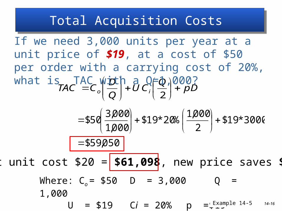
Total Acquisition Costs Total Acquisition Costs

DpQ

CUQ

DCTAC io

2

Where: Co = $50 D = 3,000 Q = 1,000

U = $19 Ci = 20% p =$19

If we need 3,000 units per year at a unit price of $19, at a cost of $50 per order with a carrying cost of 20%, what is TAC with a Q=1,000?

050,59$

3000*19$2

000,1%20*19$

000,1

000,350$

TAC at unit cost $20 = $61,098, new price saves $2,048

Example 14-5 14–14–1616

Price Discounts & Lot Sizes Price Discounts & Lot Sizes

• Determining best price break quantity:

1.Identify price breaks/lot size restrictions

2.Calculate EOQ for each price/lot size

3.Evaluate viability of each option

4.Calculate TAQ for each option

5.Select best TAQ option

14–14–1717

Production Order Quantity Production Order Quantity

• Production Order Quantity: most economical order quantity when units become available at rate produced

pd

UC

DCQ

i

op

1

2D = Annual DemandCo= Ordering cost

Ci = Holding cost

U = Unit costd = daily rate of demandp = daily rate of production

14–14–1818

Production Order Quantity Production Order Quantity

pd

UC

DCQ

i

op

1

2Qp= EOQ

D = 500,000Co= $2,000

Ci = 25%

U = $10d = 2,000 p = 5,000

515,3684.514,36

000,5000,2

110$*%25

000,2$*000,500*2

Example 14-6 14–14–1919

Demand During Lead Time Demand During Lead Time

• Variation can occur in both demand rates and lead times

222tdddlt dt

= standard deviation of demand during lead time

t = average lead time

= standard deviation of demand

d = average demand

= standard deviation of lead time

ddlt

2d

2t

14–14–2020

Demand During Lead Time Demand During Lead Time

Average demand is 10 units day with standard deviation of 1.5, and lead time of 10 days with standard deviation of 2.5 days

222tdddlt dt

t = 10 days

= 1.5 units

d = 10 per day

= 2.5 days

2d

2t

units4.25

)5.2(10)5.1(9 222

Example 14-714–14–2121

Determining Service Levels Determining Service Levels

• Service Level Policy: determining the acceptable stockout risk level

ddltzSS

ddlt

SS = Safety stock

z = standard deviations needed for service level

= standard deviation of demand during lead time

14–14–2222

Determining Service Levels Determining Service Levels

Standard deviation of demand during lead time is 25.4 units, acceptable stock out level is 5% (95% service level). From the z table = 1.65

ddltzSS

units42

4.25*65.1

Safety stock carrying cost:

$19 * 42 units * 20% = $159.60 year

Example 14-8 14–14–2323

Economic Order Quantity (EOQ) Economic Order Quantity (EOQ)

14–14–2424

Revisiting ROP and Average Inventory Revisiting ROP and Average Inventory

• Considering uncertainty

SS

Qinventryaverage

SStxdROP

2

ROP = Reorder point d = average lead time t = average demand SS = Safety stock Q = order quantity

542422

1000

13242)9*10(

inventoryaverage

unitsROP

Example 14-9 14–14–2525

Periodic Review Period Periodic Review Period

• Order Interval: fixed time between inventory review, on-hand level is unknown during this uncertainty period

AUPzUPdQ

tOIUP

ddlt

)(

UP = Uncertainty period

OI = Order interval

t = average lead time

d = average lead time

z = standard deviations needed for service level

= standard deviation of demand during lead time

A = inventory on handddlt

14–14–2626

Periodic Review Model Periodic Review Model

• Orders are placed every 30 days and average lead time is 9 days. Standard deviation of demand is 1.5 units.

tOIUP UP = Uncertainty period

OI = 30 days

t = 9 days

σd = 1.5 units

days39930

2)( dddlt UP

37.95.1)(39( 2

Example 14-10 14–14–2727

Periodic Review Period Periodic Review Period

• There are currently 105 units in stock

AUPzUPdQ ddlt )(UP = 39 days

OI = 30 days

t = 9 days

d = 10 units

z = 95% = 1.65

= 9.37

A = 105ddlt

units382

10597390

10539)37.9(65.1)39(10

Example 14-11 14–14–2828

Single Period Inventory Model Single Period Inventory Model

• Single Period Inventory Model: items are ordered once, and have little left over value (newsvendor problem)

• Target Service Level: probability of meeting demand

overstockstockout

stockout

overstockstockout

overstock

stockout

CC

CTSL

CTSLCTSL

tSalvagetDisposaltUnitC

tUnitpricesellingUnitC

1

coscoscos

cos

14–14–2929

Single Period Inventory Model Single Period Inventory Model

• Units cost $10 and sell for $30, unsold units have no value, and no disposal or salvage value

10$0010$

20$10$30$

os

so

C

C

overstockstockout

stockout

overstock

stockout

CC

CTSL

tSalvagetDisposaltUnitC

tUnitpricesellingUnitC

coscoscos

cos

667.10$20$

20$

TSL

Example 14-12 14–14–3030

Impact of Location on Inventory Impact of Location on Inventory

• Square Root Rule: estimation of impact of changing the number of locations on inventory

e

e

nn SS

N

NSS

e

e

n

n

SS

N

N

SS = safety stock of the new number of locations

= total number of new locations

= number of existing locations

= system safety stock for existing locations

14–14–3131

Impact of Location on Inventory Impact of Location on Inventory

• A single warehouse currently has 1,000 units of safety stock. How much is needed if a second warehouse is added?

e

e

nn SS

N

NSS

e

e

n

n

SS

N

N

SS = safety stock of the new number of locations

= 2

= 1

= 1000

410,1

10001

2

x

Example 14-13 14–14–3232

Inventory and Locations Inventory and Locations

14–14–3333

Reducing Inventory Costs Reducing Inventory Costs

• Managing Cycle Stock: reducing lot sizes

• Managing Safety Stock: using ABC analysis and reducing lead time

• Managing Locations: balance inventory, lead time and service levels

• Implementing Inventory Models: matching management system to specific items

14–14–3434

Independent Demand Inventory Planning Summary

Independent Demand Inventory Planning Summary

1. Determines how much and when to order

2. Continuous systems monitor on-hand levels

3. Safety stock levels are linked with service levels

4. Periodic systems count inventory at specific intervals

5. Inventory policy parameters vary by model

6. Production and economic order quantities are similar

7. Number of storage locations impact inventory levels

8. Managers should work to reduce inventory levels14–14–3535