6

Cladistics

(Attempting to reconstruct the past)

The topic of biological classification is not concluded at all by the previous two chapters.

Note, however, that the methodology discussed thus far applies outside biology as well, for

example, to the classification of thumbnails, ceramic pots, automobiles or towns, that is, prac-

tically to any inanimate objects described in terms of many variables. This general validity of

clustering has serious consequences as to the biological relevance of results: the evolutionary

relationships considered central in importance in systematics are not disclosed. This is not to

say that some hierarchial clustering methods cannot be used to produce an hypothetical evolu-

tionary tree (see Section 6.2, for details), but this is not the explicit objective of the analysis (as

in numerical taxonomy). This chapter will concentrate upon a methodological arsenal whose

primary, if not the only purpose is to reconstruct the evolutionary pathways among extant and

extinct organisms in order to provide a potential basis for their phylogenetic classification. To

achieve this goal, independence from the personal judgment of the investigator is sacrificed to

some extent, as we shall see below.

The subject matter of revealing evolutionary patterns is covered, with some generaliza-

tions, under the headline of cladistics. There is no doubt that cladistic analyses do belong to

the large family of multivariate methods, because many objects described by many variables

are involved in the study. The majority of cladistic techniques are more specialized than usual

multivariate procedures because the investigator’s assumptions on evolutionary mechanisms

are just as well, if not more important than the mathematical foundations. Contrary to the prin-

ciple implicitly or explicitly applied in the previous chapters, in cladistic studies the characters

are not equally weighted a priori: those conveying evolutionary information are used,

whereas the others are deemed to be uninformative, irrelevant and noisy. Different states of

the same character are also of unequal importance in an evolutionary perspective. Further,

cladists may also declare that, disappearance of a state during the evolution of a given group

means that it cannot appear again. We may assume with good reason that certain specific mor-

phological or physiological characters have a very little chance to develop along two inde-

pendent evolutionary lineages, and so on. This enumeration is incomplete but illustrates

sufficiently that the results depend upon our assumptions on the process of evolution, espe-

175

cially as they are applied to the particular group of organisms we are investigating. The biolo-

gist must make many decisions, most of them not merely technical, before launching a

tree-making computer program. A cladistic analysis is not a black-box procedure where sim-

ple input of data is satisfactory enough to get the final answer; being in sharp contrast with

other areas of multivariate analysis in which we are almost always faced with such a danger.

A most significant feature of cladistics is that reconstruction of past events is attempted based

on the actual properties of extant organisms,1

and the result can never in the future be con-

firmed or falsified on purely scientific grounds. Thus, it is not surprising that cladistics incor-

porates several alternative and sometimes conflicting branches whose representatives may

often go beyond plain scientific arguments (Gould, 1983, characterized some representatives

of cladistics to be the “most contentious scientists” in biology). It is therefore uneasy to com-

press the topic into a single chapter, but I feel that the basic principles and the underlying

methodology need to be mentioned in this book. Several thick volumes would be necessary to

cover the topic more completely, provided that someone were able to comprehend this com-

plex area intermingled with difficult philosophical argumentation (Stuessy, 1990, is in doubt

if such a summary is possible at all). This chapter provides many references so the reader can

proceed towards any particular direction.

The topic of cladistics may also attract attention of people not interested directly in biolog-

ical evolution. The methods can just as well be applied to other fields of science in which his-

torical events and reconstuction of past changes are to be deducted from contemporary

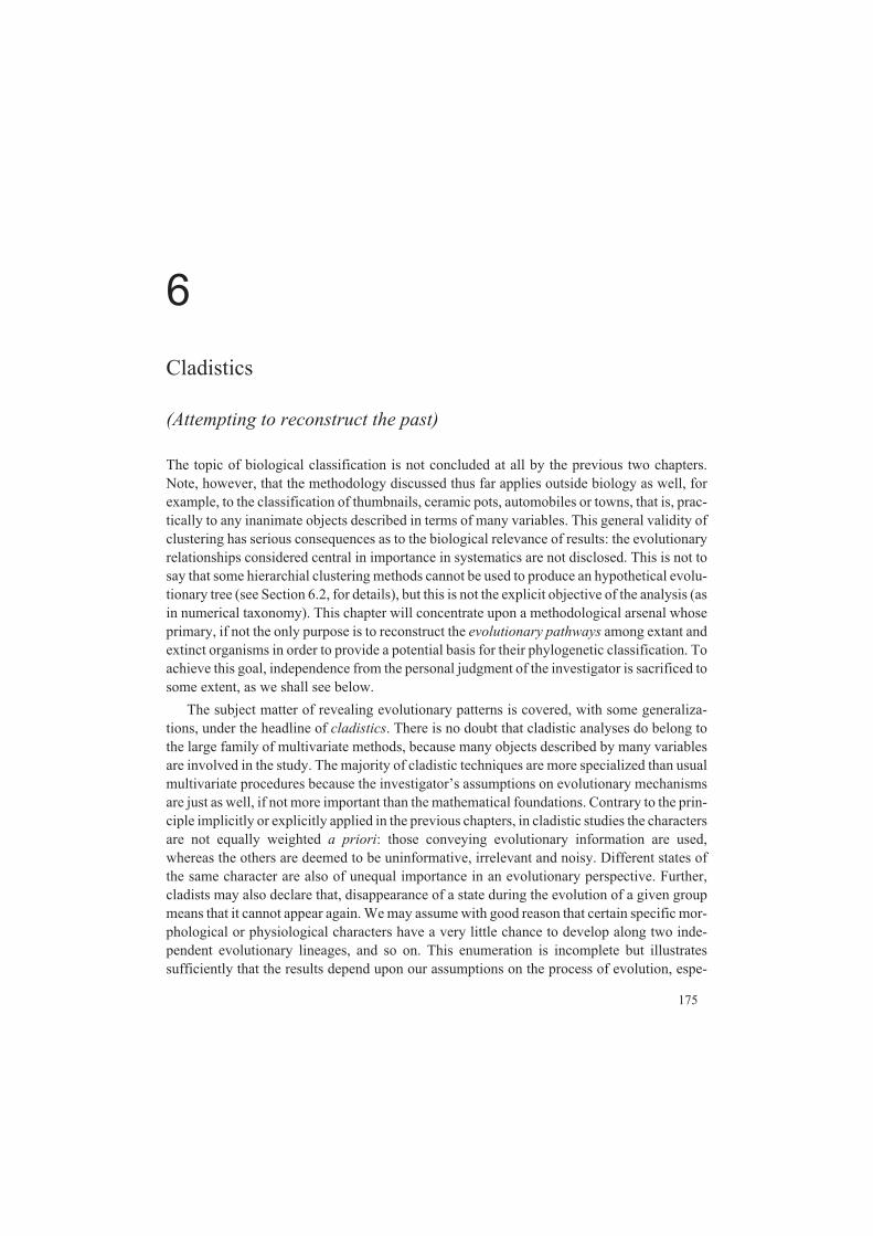
information. Such a discipline is linguistics which already has attempted to generate an evolu-

tionary tree of languages (for example, Cavalli-Sforza et al. 1988). Comparison of this lin-

guistic tree with genetic trees (Fig. 6.1) allows some conclusions to be made on the linguistic

and anthropological coevolution of human populations (Penny et al. 1993). This is mentioned

to raise interest in cladistic analysis in general, and to demonstrate its unexpectedly wide ap-

plicability in science and humanities.

6.1 Basic principles and terms

The key-stone of any cladistic approach is that evolutionary relationships can be depicted in

terms of tree graphs or, simply, trees. There is little surprise in this for a biologist if we recall

that the only illustration in Darwin’s (1859) revolutionary book was a ‘phylogenetic’ tree. Es-

sentially, in revealing evolutionary relationships one is supposed to think in terms of trees

(“tree thinking”, O’Hara 1988) at any level (even for genes within the same population).

These trees are generally termed the cladograms (clados = ‘branch’ in Greek, cf. Camin &

Sokal 1965), and their most common visualization was already shown in Fig. 5.1c. A

cladogram may also be drawn in other ways, usually with its ‘foliage’ upwards or even in a

circular arrangement. In any case, cladists are usually very careful in making distinction be-

tween their trees and dendrograms (or ‘phenograms’) as shown in the previous chapter, thus

emphasizing paradigmatic differences between numerical taxonomy and cladistics.

176 Chapter 6

1 A relatively new approach is stratocladistics (Fisher 1992) in which stratigraphic information from temporal

sequences is also considered.

The leaves of the cladogram, that is, its terminal nodes correspond with the taxa studied, in

the terminology of numerical taxonomy, with the OTUs (‘operational taxonomic units‘,

Sneath & Sokal 1973) or, which is more consistent with the objectives of cladistics, with the

EUs (‘evolutionary units‘, Estabrook 1972). The interior nodes (vertices) of the graph repre-

sent ‘extinct’ evolutionary units whose existence in the geological past is mostly hypothetical

(hence their name: HTU-s, ‘hypothetical taxonomic units‘, Farris 1970), except when we have

a good reason to include an observed taxon as an interior node. The first (in Fig. 6.2, the low-

est) interior node shows the position of the root, which is the youngest (most recent) common

ancestor of all taxa depicted by the cladogram. Contrary to dendrograms, however,

cladograms may happen to be unrooted, since determining the position of the common ances-

tor is usually the most uncertain phase of cladistic reconstruction (more details will be given

below). The edges of a rooted cladogram indicate the evolutionary pathways, in other words,

they express the ‘ancestor � descendant’ relation (the rooted tree is therefore directed, even

though the direction of edges is never shown on cladograms).

Cladistics 177

Figure 6.1. Cladograms of human popula-tions based on genetic (a) and linguistic (b)information, after Cavalli-Sforza et al.(1988) with modifications by Penny et al.(1993). The position of the root is un-known, even if we are tempted to locate aroot into the centre. Abbreviations: Mb:Mbuti (pygmy), WA: W-African, Ba:Bantu, Ni: Nilean-Saharan, S: San(bushman), Et: Ethiopian, Be: Berber, Ir:Iranian, SA: SW-Asian, Eu: European, Sd:Sardinian, I: Indus, D: Dravida (S.-Indian),L: Lapponic, U: Uralian, Mo: Mongolian,Ti: Tibetan, K: Korean, J: Japanese, A:Ainu (small people in Japan), NT: N.Turkic, Es: Eskimo, Ch: Chukch, SI:S.-American indian, KI: Central-Americanindian, NI: N.-American indian, Na:Na-Dene (an American indian people), SC:S. Chinese, MK: Mon and Khmer (fromIndochina), T: Thai, Is: Indonesian, Ma:Malayan, Ph: Philippino, P: Polinesian, Mi:Micronesian, Me: Melanesian, NG: NewGuinean, Au: Australian natives.

Most cladograms are dichotomous: each ancestor necessarily evolves into two descendant

taxa. For some cladistic approaches, dichotomous branching is a rule and cladograms contain-

ing trichotomies and multiple branchings (such as those in Fig. 6.1b) are considered unre-

solved (politomic trees, Wiley 1981.) Tree graphs contain no circles, i.e., the branches cannot

join again, so that ‘reticular evolution’ cannot be depicted by cladograms – even though we

are aware that such anastomosing events are by no means uncommon (think, for example, of

hybridization and other possibilities of gene interchange at low taxonomic levels, see Sneath

& Sokal 1973: 352-356). Consequently, the cladistic methodology is best suited to situations

where all evolutionary pathways have been stabilized and is less adequate at the population or

slightly higher levels where evolution is still ‘at work’. At very high level, strictly dichoto-

mous branching may also be unreasonable, because of the gene transfer between bacteria,

archaea and eukaryotes (reticulated tree or ‘net’, Doolittle 1999). Indeed, cladistics offers

tools for revealing evolutionary processes at the intermediate level so that ‘tree thinking’ may

not always be the most appropriate.

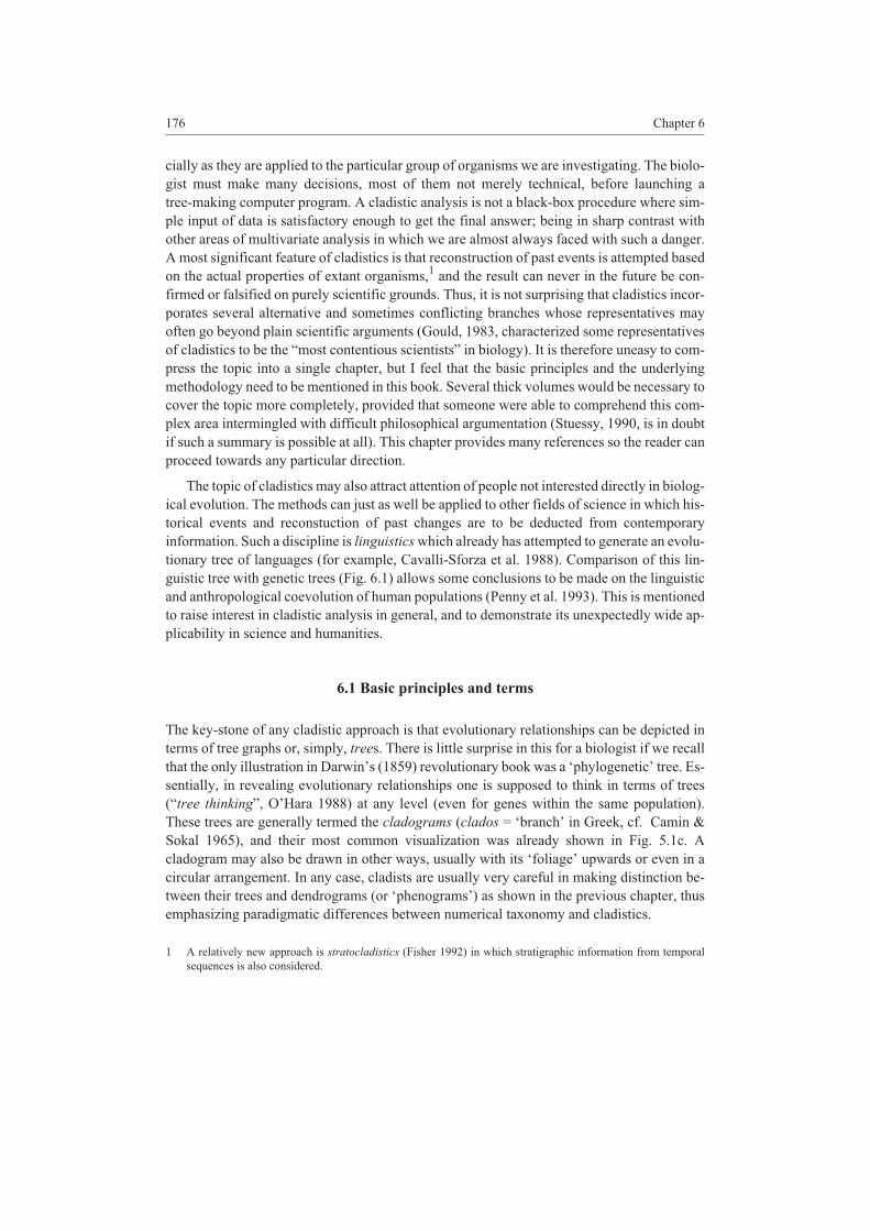
Any subtree of the cladogram is called the clade. All OTUs on the terminal branches of the

same clade comprise a monophyletic group (Fig. 6.2a), i.e., a group originating from the same

common ancestor. The other clade evolving from an ancestor right before that common ances-

tor is a sister group, such as the people of New Guinea and Australia for the remaining Pacific

and Asian groups in Figure 6.2b. In cladistic terminology, the term monophly is reserved for

groups that contain all the descendants of the common ancestor, and the exclusion of a single

OTU leads to a paraphyletic group (Hennig 1966). No question that this strict usage of the

word is contradictory with earlier definitions. For the followers of the ‘phylogenetic’ schools

of taxonomy the presence of a common ancestor for a group was a sufficient condition of

monophyly of that group, regardless whether there were other descendants from that ancestor

(Mayr 1942). Ashlock (1984) attempts to solve the dilemma by introducing the term

178 Chapter 6

Figure 6.2. Evolutionary relationships among taxa. Ina monophyletic group of the strictest cladistic sense(a: left) all descendants are included. A paraphyleticgroup (a: right) does not contain all descendants of thecommon ancestor. In a polyphyletic group some im-mediate ancestors are missing (b).

holophyletic, referring to all the decendants of an ancestor; a terminology accepted by many

taxonomists (Stuessy 1990).

To complicate things even further, the frequently mentioned polyphyletic groups also de-serve our attention, since the literature of cladistics is not harmonized at all as to the meaningof polyphyly. The polyphyletic group of Figure 6.2b corresponds with the agreeable definitiongiven by Farris (1974). At first glance, however, one could argue that this polyphyletic groupis in fact paraphyletic, since there is a common ancestor, and it is true also that some of itsdecendants are excluded from the group. There is a big difference: in the polyphyletic groupsmaller groups are joined whose immediate ancestors may not necessarily be there – unlike inthe paraphyletic groups.

One might ask the question: why this terminological argumentation? The answer is easy ifthe origin of a group is evaluated from the viewpoint of taxonomy. If we maintain the basicprinciple of systematics that the classification of living (and extinct) organisms should bebased on their evolutionary relationships (most biologists accept this view), then it becomesfairly obvious that holophyletic groups are the best defined, then follow the paraphyletic taxa,whereas polyphyletic groups are really the most problematic. The traditional classificationthat we know since our childhood, however, proves in many parts to be para- and evenpoly-phyletic under strict cladistic revision and scrutiny. This is illustrated wittily by Gould(1983) on the example of fishes. This group understood in the colloquial sense is polyphyleticcladistically, because the crossopterygians (e.g., Latimeria chalumnae from the Indian Ocean)are much closer to the quadruped terrestrial vertebrates than to the ‘other’ fishes, no matterhow fish-like these living fossils appear. The controversy is there because the term fish re-flects only very superficial macromorphological similarities. In Gould’s book, there are fur-ther examples illustrating the problem for lower taxonomic levels. The definition of zebra, asa monophyletic group, is also questionable because many bone characters suggest that horseis inserted among zebra species in the cladogram of the genus Equus. Brown bear is also aparaphyletic taxon, because polar bear, a different species, is closer to some brown bear racesthan the most different brown bear subspecies to each other (Talbot & Shields 1996).

2

What follows is perhaps the most fundamental principle of the cladistic approach. It is

generally accepted in biology (and in other fields of science as well) that simple hypotheses

are preferred against more complex ones when explaining natural phenomena. This view is

expressed here in the principle of minimum evolution. Its essence is that an evolutionary tree is

optimal if the total number of changes along the branches is the minimum. This is easily un-

derstood in case of distance-based methods which always attempt to minimize distances any-

way, and is of central importance in character-based cladistics as well. In the latter case, we

usually say that the most parsimonious cladogram is sought. The term parsimony, however,

may be easily misunderstood, because the evolutionary processes themselves are not parsimo-

nious at all, along the evolutionary routes nothing is minimized, of course. Parsimony merely

reflects our inability to find other simpler hypotheses to explain the evolutionary processes

that led to the differences among taxa in the group being investigated.3

The most detailed dis-

Cladistics 179

2 For more details on the importance of paraphyly in taxonomy see, for example, Brummitt (1997).

3 In the nucleotid sequence of a certain gene, for example, the presence of A in position 10 in the ancestor, and G in

the descendant does not mean that there was no other nucleotid change (a point mutation) at this point in the past.

The final cladogram cannot suggest more than a single change, of course. There are backward substitutions

introducing more noise in phylogenetic inference. This uncertainty is equally present in all positions and all

branches of the tree, so that the parsimony principle offers a reasonable solution of our problem (see next

subsections). Nevertheless, this is not the only possibility, suffice to mention the maximum likelihood method.

cussion of philosophical and biological aspects of parsimony is found in Sober (1983, 1988,

see also Kluge 1984).

6.2 Distance-based cladistics

The discussion of methodological details begins with techniques that utilize the concept of

distance among taxa. These methods have close relationship with the hierarchical clustering

methods discussed in Chapter 5. Therefore, the question immediately arises in a data analyst:

why not to apply hierarchical classification algorithms to estimate phylogenies based on a

wise selection of characters and a carefully chosen genetic or other meaningful distance func-

tion? For many cladists, however, this possibility does not even exist, whereas others appear

less restrictive. In accordance with my views, representatives of the latter group argue that at

least the unweighted pair group strategy (UPGMA) is worth trying simultaneously with other

cladistic methods (UPGMA clustering is offered by certain cladistic computer program pack-

ages, such as PHYLIP, Felsenstein 1993). The strongest argument against the use of cluster-

ing methods in cladistic studies is that a dendrogram implies the same distance of all OTUs

from the root, as a result of the ultrametric condition ‘forced upon’ the taxa. Evolutionary biol-

ogists are in doubt that the rate of change is constant from the ancestor along all lineages, even

though the time elapsed is the same4. To allow varying evolutionary speed in a group, the

ultrametric condition needs to be replaced by other optimality criteria. One example is the best

approximation to an additive tree. This section provides an overview of such techniques, ei-

ther with detailed description of their algorithms or merely relying upon a short description of

the fundamentals. When we attempt to reconstruct an evolutionary tree, we must keep two

things in mind: the branching pattern of the cladogram (i.e., the topology of the tree) and the

distances assigned to the branches as weights. The simultaneous optimization of these two cri-

teria is not an easy task, and it is the manner of optimization in which the methods differ most

substantially. Several algorithms yield an unrooted tree first, and then subsequent positioning

of the root provides the cladogram.

Additive trees are greatly emphasized in the reconstruction of evolutionary pathways. If

all genetic changes were completely known, then their summary would certainly produce a

perfectly additive tree: the true phylogenetic tree is additive. We do not, and cannot know all

the changes, however, only the taxa as the ‘final results’ of these changes. The distances mea-

sured among them are therefore no more than estimates of the true evolutionary distances, and

these convey the only available information to build the additive tree.

6.2.1 Minimizing the sum of branch weights (tree length)

One of the oldest propositions to represent evolutionary distances by trees is due to

Cavalli-Sforza & Edwards (1967). They introduced the concept of minimum total branch

lenght (or simply, tree length). The optimum is obtained as a minimum spanning tree (subsec-

180 Chapter 6

4 This statement is case-dependent, of course. In the literature of molecular genetics, we find many studies in

which the assumption of equal mutational change along all branches is plausible, that is, there is a ‘molecular

clock’ for all taxa. In such cases, UPGMA is a valid choice (Degens 1983, Nei et al. 1983; for examples, see

Miyahara et al. 1992, Adegoke et al. 1993). In general, the molecular clock is a reasonable assumption for closely

related taxa.

tion 5.4.3) determined for m OTUs plus many HTUs. For unrooted trees (i.e., with m–2

HTUs), the task is to minimize the sum of 2m–3 branch lengths. The original algorithm is

complicated and difficult to follow, and is not presented here. Fortunately, Saitou & Imanishi

(1989) have developed a more efficient algorithm, described as the ‘minimum evolution

method‘ by Nei (1991, see also Nei 1996). If the starting matrix of distances satisfies the con-

ditions of a four-point metric (inequality 5.11), then the resulting tree will be additive.

The ‘fault’ of dendrogams, i.e., the assumption of constant evolutionary change is cor-

rected ingeniously by the neighbor joining (NJ) method proposed by Saitou & Nei (1987),

which also belongs to the family of minimum evolution procedures (Nei 1996). In addition to

finding the smallest dij values of the matrix, as usual in clustering, the choice of the nearest

two taxa is also influenced by their average distances from all other taxa. The larger the aver-

age distances, the smaller this modified distance, because high averages imply high-speed

evolutionary divergence from the rest of the taxa, thus increasing the relative closeness of the

two taxa in question. The tree is built by an algorithm fairly similar to agglomerative hierar-

chical methods, because the D distance matrix is reduced in size step by step. As a final result,

the total tree length is optimized. The NJ method has the advantage of being much faster and

simpler than other minimum evolution methods (Nei 1991). The algorithmic steps are as fol-

lows (after Swofford & Olsen 1990).

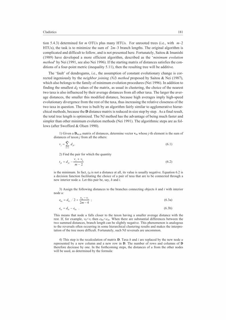
1) Given a Dm,m matrix of distances, determine vector vm whose j-th element is the sum ofdistances of taxon j from all the others:

v dj

k

m

jk��

�1

. (6.1)

2) Find the pair for which the quantity

t dv v

mjk jk

j k� �

�

� 2(6.2)

is the minimum. In fact, tjk is not a distance at all, its value is usually negative. Equation 6.2 isa decision function facilitating the choice of a pair of taxa that are to be connected through anew interior node u. Let this pair be, say, h and i.

3) Assign the following distances to the branches connecting objects h and i with interiornode u:

e dv v

mhu hi

h i� ��

�2

2 4; (6.3a)

e d eiu hi hu� � . (6.3b)

This means that node u falls closer to the taxon having a smaller average distance with therest. If, for example, vh<vi then ehu<eiu. When there are substantial differences between thetwo summed distances, branch length can be slightly negative. This phenomenon is analogousto the reversals often occurring in some hierarchical clustering results and makes the interpre-tation of the tree more difficult. Fortunately, such NJ reversals are uncommon.

4) This step is the recalculation of matrix D. Taxa h and i are replaced by the new node urepresented by a new column and a new row in D. The number of rows and columns of Dtherefore decrease by one. In the forthcoming steps, the distances of u from the other nodeswill be used, as determined by the formula:

Cladistics 181

dd d d

ukhk ik hi�

� �

2(6.4)

If we turn back to Table 5.1, then we verify easily that the above formula corresponds to therecurrence criterion of single linkage (nearest neighbor) clustering (with different indexing).

5) If the size of D is larger than 2�2, then return to step 1. Otherwise, there is only onebranch length to determine, for the last connection to be established between the remainingtwo nodes. This value is simply ehi = dhi.

If all distances in the matrix satisfy the additivity conditions (as they do in matrix 5.10),

then a perfectly additive tree is produced by NJ clustering. In other cases, the NJ tree can only

be an aproximation to an additive tree. The resulting graph is unrooted, showing evolutionary

pathways without the direction of ancestor/descendant relationships, since the position of the

common ancestor of all taxa is unknown as yet. The tree needs to be rooted, therefore, accord-

ing to either of the following ways:

1) We assume that the farthest object pairs diverged from the common ancestor at thesame evolutionary rate. That is, the root falls to the midpoint along the route between the mostremote taxa, hence the name: midpoint method. With this assumption in mind, however, weturn back at least partly to the concept of molecular clock, which we originally wanted toavoid.

2) Before any computations are made, we decide that the taxa comprise a holophyleticgroup, subsequently called the ingroup. We find one or more taxa that are evolutionarily re-lated to the ingroup, but this relationship is certainly weaker than the relationship between anytwo taxa within the ingroup. Logically enough, this taxon (or a set of taxa) is called theoutgroup. The computations will involve both groups. The branch connecting the outgroup

182 Chapter 6

Figure 6.3. Neighbor join-ing analysis of carnivorousmammals with the monkeyas outgroup, using theirimmunological distancematrix (Table A5). a:unrooted tree with an ar-row at the midpoint on thelongest path, b: this treeconverted to a cladogramafter rooting, c: UPGMAdendrogram which is topo-logically different from thecladogram. Note that indendrogram c the originaldissimilarity levels are di-vided by 2 so that patristicdistances will approximatethe immunological dis-tances.

with the ingroup in the resulting tree will then be used for positioning the root, that is, thecommon ancestor, with good reason. If the ingroup and outgroup taxa are mixed, rooting isstill possible, of course, but such results suggest that something is wrong with our a priori as-sumptions about ingroup/outgroup relationships and perhaps the whole study must restartwith a different arrangement. To be honest, inclusion of an outgroup introduces some arbi-trariness into the analysis. Furthemore, outgroups cannot always be defined, as the languageand genetic trees in Figure 6.1 exemplify (there is no human population which could certainlybe considered as an outgroup either linguistically or genetically).

The neighbor joining method and the determination of root position are illustrated using an

immunological distance matrix of carnivores (Table A5, Sarich 1969) with the monkey as the

outgroup.

The unrooted tree is shown in Fig. 6.3a. Its branch lengths are proportional to the originaldistances. Since the two root-positioning procedures provide similar solutions, the root nodeis located at the midpoint along the longest route (between the cat and the monkey, Fig. 6.3b).In this cladogram, however, branch lengths are no longer proportional with the original dis-tances; such a tree illustrates the branching pattern only. Note that the distance between taxaseparated only by one interior node in the tree (patristic distance) equals their original immu-nological distance. For other pairs, these distances are slightly different. In this example, totaltree length is 274 units. The UPGMA result is also illustrated (Fig. 6.3c) to facilitate compari-son.

6.2.2 Least squares methods

As a pioneering suggestion in cladistics, Fitch & Margoliash (1967) introduced the following

criterion:

FMd e

di j

ij ij

ij

c�

�

��

( )2

(6.5)

in which dij is the observed distance, eij is the patristic distance in the tree between taxa i and j,

and c = 2. The objective is to construct a tree in which FM is the minimum. Several variants of

the above formula have been suggested in the literature. The determination of the optimum in-

volves the combination of two steps: 1) for a given topology, branch lengths should be com-

puted so that Equation 6.5 provides the best fit, and 2) the topology must be modified to

minimize FM even further. Such a simultaneous optimization is not an easy task, and the orig-

inal algorithm suggested by Fitch & Margoliash could not guarantee determination of the ab-

solute optimum under all circumstances.

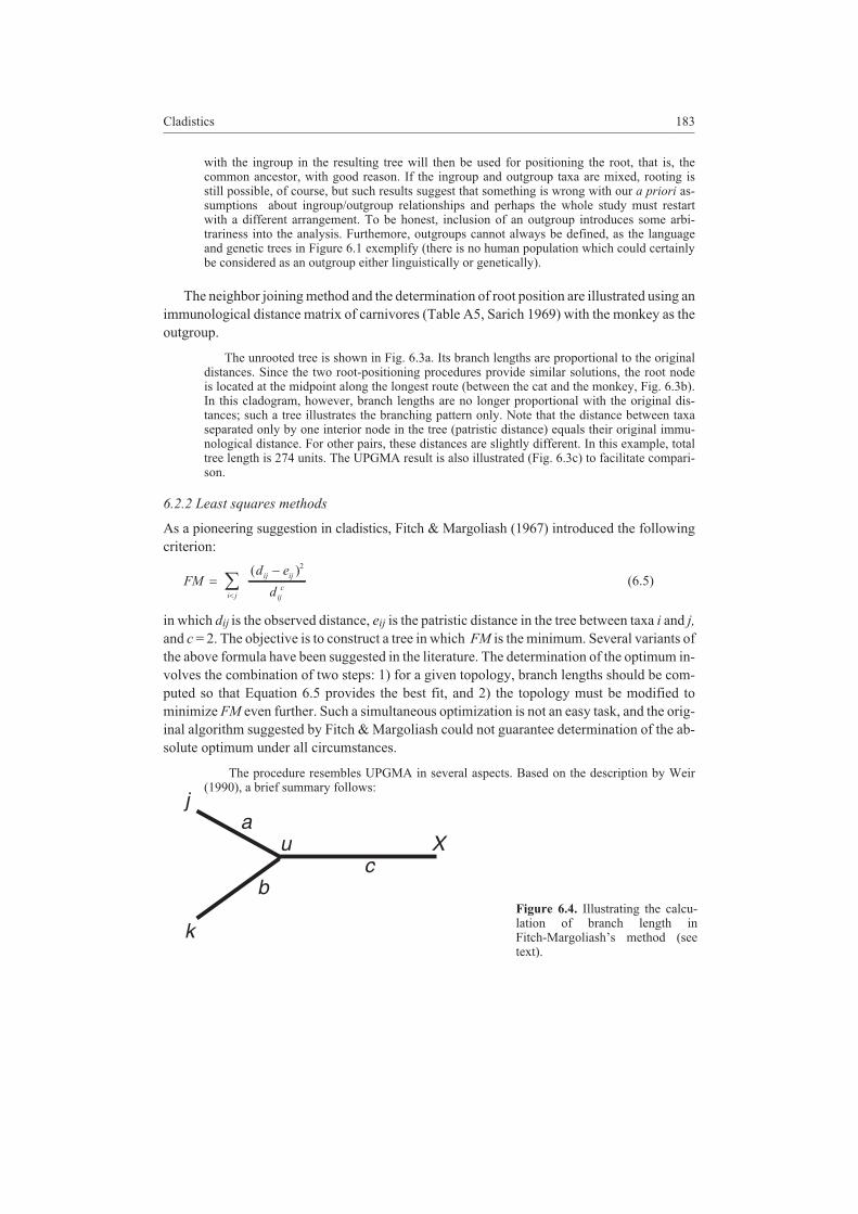
The procedure resembles UPGMA in several aspects. Based on the description by Weir(1990), a brief summary follows:

Cladistics 183

ja

u Xc

b

k

Figure 6.4. Illustrating the calcu-lation of branch length inFitch-Margoliash’s method (seetext).

1) D is used to identify the closest pair of taxa, say, j and k. A new HTU, denoted by u, isinserted between them. Then, all the remaining taxa are taken as a single group denoted by X,with nX taxa. The distance of j and k from X is defined as the arithmetic average of all dis-tances measured from j and k to the members of X:

d d n a cjX

i j k

ij X� � ��

�,

; (6.6a)

d d n b ckX

i j k

ik X� � ��

�,

; (6.6b)

djk = a + b . (6.6c)

The lengths of line segments a, b and c are sought (Fig. 6.4); they are obtained readily fromEquations 6.6a-c.

2) The distance of the new node from the taxa is calculated using the formula s =(a+b)/2. In the subsequent step, j and k are represented by u in matrix D, so its size is reducedby one column and one row.

3) The distance of u from all taxa in X is calculated in a manner well-known from thegroup average method (Subsection 5.2.1); the average of distances of j and k from a thirdtaxon, say, h is then written into the appropriate location of D.

a) If there is a single distance value in D, then subtraction of s from this distance givesthe length of the last branch, and the graph is completed.

b) In any other case, the next smallest distance is found in D and a new HTU isdetermined as described above and shown in Figure 6.4. Then, we return to Step 2.

The authors acknowledged that the topology of the tree thus obtained is not necessarily opti-

mal. Rearrangement of branches, a sort of ‘trial and error’ strategy was therefore used to im-

prove the cladogram. The ‘distances’ assigned to the branches were occasionally negative, as

in case of the neighbor joining method. Swofford & Olsen (1990: 449) provide some solutions

to this problem. For example, all negative lengths are considered to be of zero value. Recently,

the method has been scarcely used, because there are many more efficient algorithms avail-

able. It is still difficult, if not impossible however, to try all the possible topologies for more

than 20 or so taxa. The best algorithm is the one capable of examining the highest number of

cladograms in a fixed time interval.5

Cavalli-Sforza & Edwards (1967) proposed to use c = 1 in Equation 6.5, that is, they mini-

mized the plain sum of squares. The NJ method also optimizes this criterion implicitly, and the

top of it total tree length is also minimized. In addition, other values of c can be tried, thus gen-

erating a series of tree constructing methods. Felsenstein (1993) suggests that the appropriate

choice of c depends upon the errors we made when the distances were estimated. If we have a

good reason to assume that there is a constant error for all distances, no matter how large they

are, then the choice of c = 0 is appropriate. If the error variance increases along with the dis-

tances, then c should be equal to 2. The intermediate value of c = 1 corresponds to the special

case where the variance is proportional to the square root of distances.

For Sarich’s immunological distance matrix, the algorithm of Fitch & Margoliash (as im-plemented in program FITCH in the PHYLIP program package, Felsenstein 1993) produced

184 Chapter 6

5 It is therefore understandable that referees of cladistic papers require correct references to the method used as

well as to its algorithmic implementation.

practically the same tree as the neighbor joining method, after trying several hundred differenttopologies, with some slight differences in branch lengths. Of course, such a high agreementbetween different methods is case-dependent, and more differences are expected if the num-ber of taxa is much greater than eight.

6.2.3 Maximizing fit to the four-point condition

As we have seen in Chapter 5, if inequality 5.11 satisfies for all distances, then the matrix can

be perfectly represented by an additive tree. In reality, this condition rarely satisfies; the dis-

tance relations among taxa are more or less ‘distorted’. Sattath & Tversky (1977) proposed a

method (see also Fitch, 1982) that finds the best fit by optimizing tree topology first. The goal

is to find a tree in which the least number of object quadruples violate the four point condition.

After finding this topology, branch lengths are calculated according to the least squares

method (formula 6.5 with c = 1). Negative lengths are replaced by zero. The reader probably

expects that when all the distances are additive in the matrix, then the additive tree is perfectly

reconstructed.

There is more than this expectation. Gascuel (1994) compared the Sattath - Tverskymethod with the NJ technique, and provided a theoretical explanation why these two methodsprovide identical or very similar results.

6.2.4 The Wagner-distance method

The methods discussed above share the property that branch lengths, that is the estimated pa-

tristic distances can be either larger or smaller than the values in the starting D matrix. The

strategies are insensitive to the direction of deviations, and this is why negative values may

also appear. The negative scores are eliminated automatically by applying the restriction that

the starting distances are the lower bounds of the possible patristic distances. Then, a tree is

optimal if its length is the minimum provided that none of the patristic distances exceeds its

counterpart in the starting matrix. Farris (1970) proposed to call this cladogram the Wagner

tree6. To understand its algorithm, recall the minimum spanning tree (Subsection 5.4.3). In

this, each node corresponds to an OTU, so we have m-1 edges (branches) and the total length

of the tree is the minimum (for Sarich’s immunological matrix this tree has a length of 365

units). Addition of further nodes to the tree will diminish tree length, just remember the NJ so-

lution in which tree length is only 274 units. (365 units are too many even if we do not allow

patrisitic distances to be lower than the originals.) These new nodes will be the HTUs. The

method proposed by Farris is a heuristic approximation to the absolute optimum, and has sev-

eral variants (Farris 1972, Swofford 1981, Tateno et al. 1982, Faith 1985). The method applies

to Manhattan distances (Formula 3.48) only. The analysis begins with connecting the nearest

OTUs. In each further step, one OTU joins the tree such that a new HTU is defined on the

branch nearest to it.

Further details of the algorithm can be ignored here. In the above example of immunologicaldistances, Fitch (1984) determined a Wagner tree with a length of 291 units, which is cer-

Cladistics 185

6 This is Wagner tree because Farris’ strategy is a generalization of a character-based method (Section 6.3) to

continuous characters, and the character-based method was developed and first used by Wagner. If no reference

is made to distances when Wagner trees are mentioned, then the method to be discussed in Section 6.3 is used in

that paper.

tainly ‘worse’ than the NJ and the Fitch - Margoliash cladograms. As Felsenstein (1993)points out, the Wagner method is of historical importance indeed, because other algorithmsusually provide shorter trees. ‘Bad performance’ is obviously due to the restriction that patris-tic distances must not be less than the starting ones.

6.3 Character-based reconstruction of evolutionary trees

If we disregard cases where our starting data are obtained in the form of distances (e.g.,

DNA hybridization [Krajewski & Dickerman 1990], immunology), most cladists take the

view that distance methods should be neglected because too much information is lost when

distances are calculated from raw data. Their main argument is that conversion of an OTU �characters matrix into distances will mask the evolutionary changes of individual characters

(character evolution, Maddison & Maddison 1992), something considered most essential in

interpreting cladograms. Without entering into details of the controversy between the ‘dis-

tance party’ and the ‘character party’, it is fair to note that character-based cladistics treats

mostly discrete characters, and therefore its relevance is limited. (There are procedures to con-

vert continuous variables into discrete form, but then we can argue that it is this transforma-

tion that causes loss of information; that is, “what is made up on the rounds is lost on the

swings”). Of course, we can try both approaches, and even numerical classification methods

in the same study (as Duncan et al. 1980 seem to suggest) thus escaping from all controversies.

In this section, however, there will be no more mention of distances, because attention is fo-

cused on the direct cladistic exploitation of characters.

We have arrived at the true ‘hunting-ground’ of cladistics. Although Hennig (1950, 1966),

a German insectologist, is generally considered as the theoretical pioneer of the charac-

ter-based cladistic approach and the greatest figure in its history, further developments in this

area were almost entirely confined to the English speaking world. A new jargon, esoteric for

the outsider, has developed and it was the primary reason that cladistics could not grow fast

enough into a widely accepted scientific discipline. In any case, in addition to the basic princi-

ples discussed in Section 6.1, some area-specific terminology needs to be introduced.

Hennig’s original argumentation is rooted in the ‘triviality’ that during evolution the char-

acters (attributes, features) of organisms are subject to change; from an ancestral (primitive or

plesiomorph) state they develop into derived (or apomorph) state(s). There can be many de-

rived states of the same character, of course7, and in a strictly monophyletic group only a sin-

gle plesiomorph state can be allowed. The reconstruction of the evolutionary pathways

attempts to maximize the number of derived character states in which closely related taxa

agree (such an agreement was termed the synapomorphy by Hennig). That two taxa share an

ancestral state (symplesiomorphy) is immaterial for a cladist, such an agreement conveys no

phylogenetic information at all. Derived character states may also appear only on a single ter-

minal clade, this pehnomenon is called the autapomorphy.

Whether the states of a given character are primitive or derived, that is character polarity,is examined by various methods employing new ‘tricks’, as summarized below.

186 Chapter 6

7 These correspond with the states of a nominal variable, cf. Subsection 1.4.1.

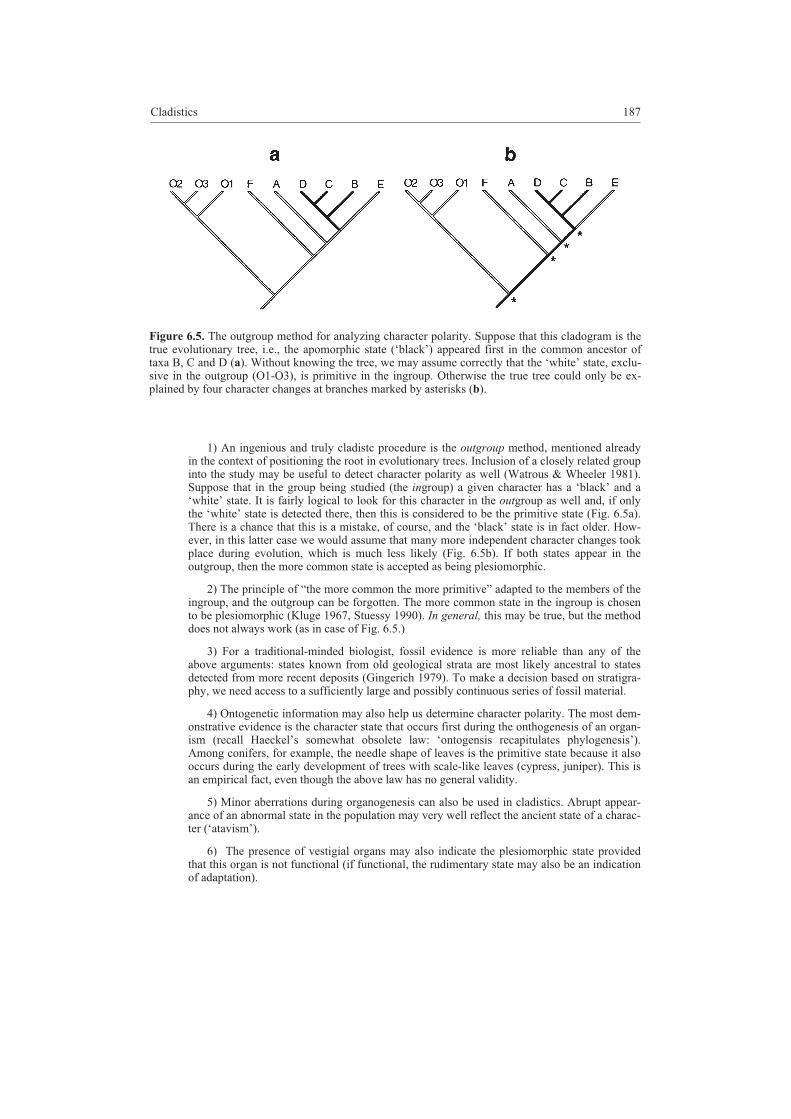
1) An ingenious and truly cladistc procedure is the outgroup method, mentioned alreadyin the context of positioning the root in evolutionary trees. Inclusion of a closely related groupinto the study may be useful to detect character polarity as well (Watrous & Wheeler 1981).Suppose that in the group being studied (the ingroup) a given character has a ‘black’ and a‘white’ state. It is fairly logical to look for this character in the outgroup as well and, if onlythe ‘white’ state is detected there, then this is considered to be the primitive state (Fig. 6.5a).There is a chance that this is a mistake, of course, and the ‘black’ state is in fact older. How-ever, in this latter case we would assume that many more independent character changes tookplace during evolution, which is much less likely (Fig. 6.5b). If both states appear in theoutgroup, then the more common state is accepted as being plesiomorphic.

2) The principle of “the more common the more primitive” adapted to the members of theingroup, and the outgroup can be forgotten. The more common state in the ingroup is chosento be plesiomorphic (Kluge 1967, Stuessy 1990). In general, this may be true, but the methoddoes not always work (as in case of Fig. 6.5.)

3) For a traditional-minded biologist, fossil evidence is more reliable than any of theabove arguments: states known from old geological strata are most likely ancestral to statesdetected from more recent deposits (Gingerich 1979). To make a decision based on stratigra-phy, we need access to a sufficiently large and possibly continuous series of fossil material.

4) Ontogenetic information may also help us determine character polarity. The most dem-onstrative evidence is the character state that occurs first during the onthogenesis of an organ-ism (recall Haeckel’s somewhat obsolete law: ‘ontogensis recapitulates phylogenesis’).Among conifers, for example, the needle shape of leaves is the primitive state because it alsooccurs during the early development of trees with scale-like leaves (cypress, juniper). This isan empirical fact, even though the above law has no general validity.

5) Minor aberrations during organogenesis can also be used in cladistics. Abrupt appear-ance of an abnormal state in the population may very well reflect the ancient state of a charac-ter (‘atavism’).

6) The presence of vestigial organs may also indicate the plesiomorphic state providedthat this organ is not functional (if functional, the rudimentary state may also be an indicationof adaptation).

Cladistics 187

Figure 6.5. The outgroup method for analyzing character polarity. Suppose that this cladogram is thetrue evolutionary tree, i.e., the apomorphic state (‘black’) appeared first in the common ancestor oftaxa B, C and D (a). Without knowing the tree, we may assume correctly that the ‘white’ state, exclu-sive in the outgroup (O1-O3), is primitive in the ingroup. Otherwise the true tree could only be ex-plained by four character changes at branches marked by asterisks (b).

7) Experience in evolutionary biology and taxonomy suggests that characters with primi-tive state have a high chance to appear together in a group, that is, they are associated. There-fore, the state of an unexamined character is likely to be ancestral, if many other charactersalso possess the primitive state in the group (Crisci & Stuessy 1980, Sporne 1976).

8) Another potentially useful method is the comparative evaluation of parallel evolution-ary trends in the group under study. An example is the secondary aggregation of head inflo-rescence in many angiosperm genera, showing that the simple head is the older state.

9) Evolutionary directionality may also be assessed by considering the geographical dis-tribution of taxa. Since more ancient taxa had more time to attain wide dispersion, the stateobserved in the most widespread taxon is considered primitive compared to states that appearin narrowly distributed species.

The above list is no more than mere illustration of the possibilities. There is no space todiscuss all difficulties, limitations and relative merits of methods that examine character po-larity. A separate chapter could be written on this topic, so the reader is referred to Stuessy(1990:106-113), Quicke (1993: 16-22), and Mayr & Ashlock (1991: 212-214) for more de-tails. As the first of the above authors pointed out, “there is no simple solution” to the polarityproblem and “no single method is the only correct one”.

In addition to character polarity, the homology of traits is to be treated with caution: one

has to make sure that agreement of character states is the result of common ancestry. In a

sense, we are now in a vicious circle, because knowledge of evolutionary relationships would

be needed to make absolutely correct statements on homology, but it is these relationships that

we are trying to derive from the characters. Nevertheless, in the majority of cases homologous

character states are easily identified using some external information. Homology is the basic

principle in numerical taxonomy as well; there is no point to consider a bird and a fly to be

similar because both have wings. A ‘sworn enemy’ of cladists is homoplasy, the opposite to

homology, where agreement in character states is not a proof of common ancestry (cf. Sander-

son and Hufford 1996). Parallel and convergent evolution may lead to identical character

states in distant groups independently, thus rendering phylogenetic reconstruction more diffi-

cult8. Another manifestation of homoplasy is when an apomorphic state is reversed to the

primitive. Most often, cladograms cannot be generated without homplasies, but the objective

is always to keep their number to the minimum.

Reversal of character states poses no problems whenever biological considerations en-

tirely exclude its possibility. Examination of polarity is therefore not enough, and the potential

directions of character change need careful scrutiny before cladistic reconstruction is

launched. The examination of possible transitions between states is yet another critical area of

cladistics and again, I give only a very brief summary of this fairly diverse and controvesial

subject matter. As we shall see, categorization of data types as given in Chapter 1 is insuffi-

cient, and further refinement and clarification of inconsistencies are in order. On the other

188 Chapter 6

8 Distinction between parallelism and convergence is neither essential for our purposes, nor is simple in many

situations. The wings of flies and birds and the succulent trunks of cacti and some Euphorbiaceae are results of

the convergent evolution of taxonomically remote groups due to adaptation, and they rarely cause any headache

for the cladist. Parallelism implies that the taxa under study ‘started’ their evolution with the same conditions

and are subject to similar influences in all times (Gosliner & Ghiselin 1984, Harvey & Pagel 1990). Examples

are morphological coincidences observed among passerine birds in different continents..

hand, cladistic terminology often coincides with the previous definitions, so the subsequent

discussion can be founded upon our existing knowledge of data types.

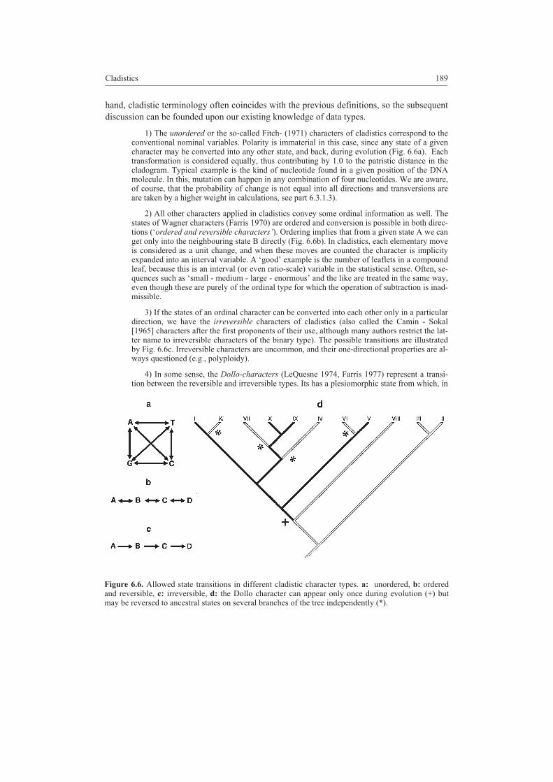
1) The unordered or the so-called Fitch- (1971) characters of cladistics correspond to theconventional nominal variables. Polarity is immaterial in this case, since any state of a givencharacter may be converted into any other state, and back, during evolution (Fig. 6.6a). Eachtransformation is considered equally, thus contributing by 1.0 to the patristic distance in thecladogram. Typical example is the kind of nucleotide found in a given position of the DNAmolecule. In this, mutation can happen in any combination of four nucleotides. We are aware,of course, that the probability of change is not equal into all directions and transversions areare taken by a higher weight in calculations, see part 6.3.1.3).

2) All other characters applied in cladistics convey some ordinal information as well. Thestates of Wagner characters (Farris 1970) are ordered and conversion is possible in both direc-tions (‘ordered and reversible characters’). Ordering implies that from a given state A we canget only into the neighbouring state B directly (Fig. 6.6b). In cladistics, each elementary moveis considered as a unit change, and when these moves are counted the character is implicityexpanded into an interval variable. A ‘good’ example is the number of leaflets in a compoundleaf, because this is an interval (or even ratio-scale) variable in the statistical sense. Often, se-quences such as ‘small - medium - large - enormous’ and the like are treated in the same way,even though these are purely of the ordinal type for which the operation of subtraction is inad-missible.

3) If the states of an ordinal character can be converted into each other only in a particulardirection, we have the irreversible characters of cladistics (also called the Camin - Sokal[1965] characters after the first proponents of their use, although many authors restrict the lat-ter name to irreversible characters of the binary type). The possible transitions are illustratedby Fig. 6.6c. Irreversible characters are uncommon, and their one-directional properties are al-ways questioned (e.g., polyploidy).

4) In some sense, the Dollo-characters (LeQuesne 1974, Farris 1977) represent a transi-tion between the reversible and irreversible types. Its has a plesiomorphic state from which, in

Cladistics 189

Figure 6.6. Allowed state transitions in different cladistic character types. a: unordered, b: orderedand reversible, c: irreversible, d: the Dollo character can appear only once during evolution (+) butmay be reversed to ancestral states on several branches of the tree independently (*).

the simplest case, only a single new state develops (Fig. 6.6d), but a series of new (derived)states can also be conceived. The new state can be reversed to any previous state simulta-neously and independently on different branches of the phylogenetic tree. In addition, thecharacter has the essential property that the derived states can appear once and only once dur-ing the evolution of the group, that is they are uniquely derived. This means that parallelismand convergence are excluded, which is a very strong condition, considered valid mostly forrestriction enzymes (Swofford & Olsen 1990). Some chemotaxonomical characters are also ofthis type; the ability to synthetize a complex secondary metabolite develops very likely onlyonce during evolution, whereas this ability is easily lost if, for some reason, the taxon is nolonger able to produce any intermedier compound in the metabolitic sequence.

5) With the above types, we implicitly assumed that all individuals of a given EU areidentical for a selected character. If several alleles of a gene appear in a population, then thecorresponding character cannot be described in terms of the above character types any longer.Therefore, the notion of polymorphic characters is introduced. The cladistic analysis of poly-morphic characters is cumbersome and sometimes impossible, and the genetic distance mea-sures based on allele frequencies are recommended instead. A more recent account of thetopic is in Wiens (1995).

6) Finally, the stratigraphic characters are mentioned. These characters convey sequential(temporal) information coming from fossil material and were first applied in cladistics byFisher (1992). The stratigraphic characters are in fact irreversible, because the descendantscannot be older than the ancestors. The state coming from the oldest stratum can be coded by0, the one detected in the next stratum by 1, and so on.

Having been familiar with the basic types of cladistic characters, we can sit down and try to con-

struct a hypothetical evolutionary tree for our study group. Two different approaches can be se-

lected for this purpose; the larger – and more important – group of procedures rely upon the

parsimony principle, whereas the smaller group includes methods evaluating character compati-

bility.

6.3.1. Parsimony methods

In general, parsimony methods attempt to minimize the total tree length of cladograms. In

other words, they look for a graph which requires the minimum number of state transforma-

tions (evolutionary steps) necessary to fully explain the evolutionary relationships within a

group of taxa. Prior to entering mathematical details of modern and relatively sophisticated

techniques, let us examine a simple example to illustrate Hennig’s original ‘manual’ ap-

proach. This way comparisons with other methods will also be possible.

Suppose that we have six taxa described in terms of eleven irreversible characters, eachwith two states. The plesiomorphic state is denoted by 0, the derived state is coded by 1 (Ta-ble 6.1). We can see at first glance that the data matrix contains several autapomorph charac-ters (1, 4, 7-11), about which we need not worry any more. For the remaining four characters,synapomorphy is identified as follows: 2: {taxa A, B}, 3: {C, D}, 5: {A, B, C, D}, and 6: {E,F}. This distribution of synapomorphic states allows the conclusion that the first dichotomyappeared between groups {A,B,C,D} and {E,F}. The latter group is the closest to the hypo-thetical common ancestor described entirely with 0 states; they differ only in characters 1 and2. Characters 2 and 3 show unequivocally that the subsequent split separated taxa {A,B} from{C,D}. Then, we have the trivial job of dividing the three two-member groups even further, toobtain the cladogram of Figure 6.7a. Numbers on the branches identify characters thatchanged there. The sum of state changes over all branches is the tree length, which happens tobe equal to the number of characters, i.e., 11. After some rearrangements of the tree, one caneasily see than any other topology would require more changes, in fact, homoplasies.

190 Chapter 6

An alternative to the numbered cladogram is Wagner’s (1961) ‘groundplan/divergence’display. The centroid of concentric semi-circles represents the hypothetical common ancestor,and each centripetal move indicates a single character state change. Empty symbols areHTUs, full symbols are OTUs. The extent to which an OTU deviates from the common ances-tor is better reflected in this diagram thain in a cladogram (the additivity of branch lenghts isshown). It is also seen that taxon E did not even change after its divergence from taxon F, andcan be considered to be its ancestor.

This example was deliberately simple so that tree construction was an easy task. The tree with

the minimum number of steps and without homoplasies was found easily. In practice, how-

ever, we are faced with much more difficult situations because the number of characters and

OTUs is generally higher. Furthermore, it is rarely the case that the tree can be constructed

without homoplasies. If, for instance, character 1 for OTU A is modified to state 1, then the

problem becomes more difficult to handle: taxa A and D are on different branches on the

cladogram of Fig. 6.7a, and according to this topology the autapomorphic state of character 1

had to develop twice during evolution. This is a typical homoplasy. After modifying the topol-

ogy such that A and D get closer to each other, so that this homoplasy is removed, then charac-

ters 2 and 3 will be problematic. A plausible ‘solution’ is to discard character 1 entirely, which

is not always a good strategy to follow – and leads to methods to be discussed in Subsection

6.3.2. Parsimony methods, however, tolerate the presence of homoplasies. Hennig and Wag-

Cladistics 191

Characters

OTUs 1 2 3 4 5 6 7 8 9 10 11 S�

A 0 1 0 0 1 0 1 1 0 0 0 4 2

B 0 1 0 1 1 0 0 0 0 0 0 3 1

C 0 0 1 0 1 0 0 0 0 1 0 3 1

D 1 0 1 0 1 0 0 0 1 0 0 4 2

E 0 0 0 0 0 1 0 0 0 0 0 1 0

F 0 0 0 0 0 1 0 0 0 0 1 2 1

Table 6.1. Artificial data matrix to illustrate Hennig’s method. The penultimate column shows thenumber of derived states, the last column indicates the number of autapomorphies for each taxon.

Figure 6.7. Cladogram constructed from the data of Table 6.1 by Hennig’s method (a) and the corre-sponding groundplan/divergence diagram (b).

ner were not in a position to find the most parsimonious tree given many homoplasies; they

could only dream of high-speed computers. Modern computer technology and the current

state of optimization algorithms increase the chance of finding the most parsimonious tree for

a given group of OTUs, even though for large problems we can never be sure that the final re-

sult is the absolute optimum (see below).

According to Swofford & Olsen (1990), parsimony methods are designed to select tree �from the set of all possible trees such that the optimality criterion given below is minimized:

L w x xk

N

j

n

j k j k j

B

( ) ( , )� � � �

� �1 1

1 2� (6.7)

where NB is the number of branches, n is the number of characters, xk1j and xk2j are the states

of character j for the two nodes at the endpoints of branch k, wj is a weight expressing the im-

portance of character j (usually 1), and �(xk1j, xk2j) is the ‘cost’ of the transition between the

two states. These states may correspond to a score actually appearing in the data (for a given

OTU) or are hypothetical values assigned to interior nodes (HTUs). The quantity L(�) mea-

sures tree length, a term already mentioned several times. The length and the topology of the

optimal tree9

depend on admissible state transitions and the cost function. The job consists of

a double optimization, as in case of distance methods: 1) character states that minimize tree

length for a given topology are assigned to the interior nodes, and 2) the topology is optimized

in order to allow more optimal character state assignments. The modification of tree topology

usually follows the same strategy, regardless the type of characters, but the assingnment of

states to interior noda must accord with the properties of each character: different types re-

quire different algorithms.

6.3.1.1 Optimizing tree length

Given the states for OTUs at the terminal branches of the tree, the aim is to determine the

states of character h for each HTU such that tree length is minimized. This process is called the

tree reconstruction. For unordered and Wagner characters, due to the reversibility of their

states, the position of the root does not affect the result – a fact utilized heavily during the anal-

ysis. The optimization algorithm is illustrated after Swofford & Maddison (1987) in a strongly

simplified form for the unordered (Fitch-) type and for strictly dichotomous (fully resolved)

trees. The essence of the algorithm is that an OTU is chosen to be the root, and the tree is

scanned from all other taxa to the root and back. If there is an OTU that represents an

outgroup, then it is the best choice for rooting. During the first scan, possible states are de-

tected for each interior node and, in the second phase when the tree is examined backwards,

we decide which states are retained.

1) Obviously, for the OTUs the states are fixed, whereas for the HTUs there are no start-ing states. Temporarily, HTUs can have more than one state in the first pass. Let g be the rootnode. For character h, tree length is Lh = 0 at the outset.

2) Find interior node k whose both descendants have known states. Let these adjacentnodes be denoted by i and j. Then, we have to make a choice from two possibilities:

192 Chapter 6

9 The optimality criterion 6.7 may be satisfied by several, even hundreds of trees, which may differ from one

another considerably. In such cases, consensus methods to be discussed in Section 9.4 will offer a solution.

2a) if there are states in which i and j agree, then all these states are assigned tonode k;

2b) if there is no such state, then all states belonging to i and j are assigned to k, and Lh

is increased by one.

3) If k happens to be the direct descendant of g, then proceed with step 4. Otherwise, re-turn to step 2.

4) If the character state for g does not agree with any state of its immediate descendant,then Lh is increased by 1. The first pass is now completed, and the value of Lh is the treelength for character h. Then, starting from the root we determine appropriate character statesfor the HTUs.

5) Select an interior node k for which the state of character h is not yet final, but that of itsimmediate ancestor, denoted by o, is known. (That is, first we examine the node nearest to theroot).

6) If the character state belonging to o is also assigned to k (possibly among others), thenthis is chosen to be the final state for node k. Othwerwise, one of the states pertaining to k ischosen arbitrarily and retained.

7) When the examination of all interior nodes is completed, the search is finished. Other-wise return to step 5.

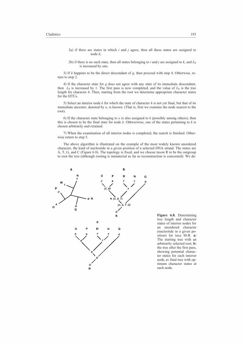
The above algorithm is illustrated on the example of the most widely known unorderedcharacter, the kind of nucleotide in a given position of a selected DNA strand. The states areA, T, G, and C (Figure 6.8). The topology is fixed, and we choose taxon R to be the outgroupto root the tree (although rooting is immaterial as far as reconstruction is concerned). We de-

Cladistics 193

Figure 6.8. Determiningtree length and characterstates of interior nodes foran unordered character(nucleotide in a given po-sition) for taxa M-R. a:The starting tree with anarbitrarily selected root, b:the tree after the first pass,showing potential charac-ter states for each interiornode, c: final tree with op-timum character states ateach node.

termine tree length and the potential character states of interior nodes according to steps 2-4.(Fig. 6.8b). The first scrutiny of the tree indicates that changes must appear along threebranches so L = 3. The remaining task is to assign character states to the interior nodes, as il-lustrated by Figure 6.8c. In the position denoted by an *, we made an arbitrary decision, nev-ertheless, one may easily verify that any other choices would provide the same tree length.Owing to the ambiguities involved in our choices, the same topology may have several recon-structions

10

For Wagner characters, because the order and the differences of states are both interpretable,

the above algorithm modifies in steps 2a, 2b, 4 and 6 as follows:

2a) if the states for i and j overlap, then these shared states are assigned to interior node k(for example, if i is represented by states 1, 2 and 3 whereas j is described by 2, 3 and 4, thenthe combination assigned to k is chosen to be 2, 3). .

2b) if there is no overlap, then the two nearest states and their intermediates are assignedto k and L is increased by the difference between the nearest two states (e.g., let i be 1, 2, 3and j be 5,6, then the temporary combination for k is given by 3,4,5 and Lh increases by 2)

4) If the state of g does not agree with any states of its immediate descendant, then thenew value of Lh is Lh+ | state in g – the nearest state in the descendant | .

6) of the states pertaining to k the one nearest (or equal) to the state for o is retained.

All this becomes clear if we consider the example of Figure 6.9. Assume that six taxa aredescribed in terms of an ordered reversible character with four possible states, coded by 0, 1,2 and 3 (Figure 6.9a). Taxon R is taken as the root and, in the first pass, temporary charactercombinations are assigned to the interior nodes (Fig. 6.9b). The operations in step 2a) are ap-plied to set states 3 and 2 fixed, and those in step 2b) lead to the choice of combinations (0,1)and (1,2,3). In the backward direction, the remaining ambiguities are resolved to obtain the fi-nal reconstruction in Figure 6.9c. Tree length is 4 units for this character.

Afterwards, the above procedure is performed for every other character as well, and then Lh

will give total tree length. Characters of different type are allowed to appear simultaneously in

the data.

The parsimony methods suitable to the remaining character types (e.g., Dollo) and to the

generation of politomic trees are much more complicated and are not discussed here. They

cannot be applied without computer programs, so the reader is referred to the user’s guides for

details (e.g., Maddison & Maddison 1992, Felsenstein 1993).

6.3.1.2 Optimizing the topology of evolutionary trees

Finding the most appropriate character states for all interior nodes of the tree is the easiest part

of the job. Criterion 6.7 is much more influenced by the topology of tree branches than by the

assignment of states. Seeking the optimum topology raises further difficulties, as we shall see

from the following brief discussion.

194 Chapter 6

10 Noted are the ACCTRAN and the DELTRAN choices, as two extremes. In the first case, changes are allowed to

happen as close to the root as possible, so that early gains are maximized and subsequent reversals are forced. In

DELTRAN, the ancestral state is carried as far from the root as possible, thus maximizing parallel changes (see

Swofford & Maddison 1987).

Complete enumeration. As a straightforward solution, one may suggest to generate all the

possible trees and to optimize each of them for character state assignments. In this way, we

can make sure that the tree giving the absolute minimum for criterion 6.7 is found. However,

examining all possibilities is not as easy as it might seem at first glance. We mentioned in

Chapter 5 already how enormous is the number of different dendrograms for only 10 objects

if the levels are not considered (Formula 5.16). This is exactly the number of possible rooted

cladograms (for m = 10, more than 34 million). If the root is removed, then the following for-

mula applies:

i

m

mi

m

m��� � �

�

�33

2 52 5

2 3( )

( )!

( )(6.8)

(Felsenstein 1978). This quantity is still very high, exceeding two-million for 10 objects. In

actual phylogenetic studies, many more taxa are included resulting in astronomical numbers

of possible trees. Complete enumeration becomes inconceivable very quickly when m in-

creases, notwithstanding the current advancements in computer technology.

For unrooted trees, complete enumeration starts from the single possible tree for three ob-jects. In this, there are three branches. The next taxon may be positioned onto any of thesebranches, therefore we have three different arrangements for m = 4.This tree will have fivebranches, so that five is the number of possibilities to join the fifth taxon. This is multipliedby the number of possible trees for 4 objects, thus giving a total of 3�5 = 15 possible trees(Fig. 6.10). We can see that addition of every taxon increases 2i – 5 times the number of pos-

Cladistics 195

Figure 6.9. Determiningstates for interior nodes incase of Wagner characters.a-c: as in Figure 6.8.

sible trees obtained in the previous step (i is the number of taxa in the given step) – so that themeaning of Formula 6.8 becomes clear.

Exact methods. There is an obvious need for algorithms that are not exhaustive, yet the opti-

mum result is produced within a reasonable time. The branch and bound algorithm mentioned

in Subsection 5.3.1 is a case in point. Its first application to cladistic analysis is due to Hendy

& Penny (1982). At the outset, we select a reference tree generated by some heuristic method,

to be discussed later, so it is expected not to be very distant from the optimum. Let its length be

Lmin (the ‘bound’). Then, we start the iterations from ‘zero’, as if complete enumeration were

intended. Tree length is evaluated in the meantime for all subtrees and when Lmin is exceeded

the search stops in this direction (‘branch’) because in the further steps tree length can only in-

crease resulting in even worse solutions. Every tree containing that long subtree is discarded

automatically during the analysis. If a full tree is built up such that its length is shorter than

Lmin, then this new tree becomes the reference basis. This description is very far from being a

complete presentation of the algorithm, but the reader hopefully sees that in the worst case the

branch and bound method equals complete enumeration. If the starting value of Lmin is close

to the absolute optimum, the method is far more efficient than exhausive search. However,

computing time increases rapidly when m increases, and the best implementations of the algo-

rithm can find the optimum only for 20-30 taxa.

That is, for 100 taxa or more, the branch and bound method cannot guarantee that the op-timization ends within reasonable time. Unfortunately, we do not know yet any exact algo-rithm that produces the optimum tree regardless the number of taxa involved. Finding the besttopology is in fact an NP-complete problem, a general algorithmic property examined very in-tensively in mathematics (Graham & Foulds 1982). An inherent feature of any optimizationalgorithm is the dependence of computing time on problem size, m. For the majority ofmultivariate data analysis methods (e.g., clustering) time is proportional to m

2or m

3, causing

no practical difficulties for the investigator even for very large m. We could tolerate timecomplexity with m raised to the power of 4, 5 or more. However, the time requirement forfinding the optimum tree becomes intractable beyond a certain limit for the number of taxa;time complexity increases in a non-polynomial manner (hence the abbreviation, NP) in thefunction of m. It has been shown that if a fast algorithm were found for any NP-completeproblem, then all the NP-complete problems could be solved by this algorithm (Lewis &Papadimitriou 1978).

196 Chapter 6

Figure 6.10. Enumeration ofall the possible dichotomouscladograms for four OTUs.

Heuristic methods. For large numbers of taxa, one has to accept the plain truth that no method

can guarantee the detection of optimal tree topology in reasonable time (Day 1983). We can

only hope that iterative strategies and heuristic searches will reach a fair closeness to the abso-

lute optimum relatively quickly. These methods resemble in several aspects the k-means

method of non-hierarchical clustering and other procedures to be discussed in the forthcoming

chapters: a starting configuration is modified in each step and the iterations stop when no fur-

ther improvement can be achieved. Since the final result may strongly depend on the starting

topology, it is recommended to try as many different initial configurations as possible. Then,

the best of the local optima thus obtained can be selected and declared to be final result – al-

though we must bear in mind that the iterations may have missed the route leading to the abso-

lute optimum.

There are two iterative strategies for cladograms. The first method involves a step-by-step

construction by adding taxa, one at a time, to small trees. At the outset, three taxa are selected

at random or by minimizing tree length. In the first step, we examine how the addition of each

of the other taxa to each existing branch would increase tree length. Then, the taxon providing

the minimum increase is retained. In the subsequent step, yet another taxon is added to the tree

in a similar way and the procedure is continued until the tree is completed. The problem with

these methods is the same as with agglomerative clustering: the position of taxa that are al-

ready added to the tree cannot be modified afterwards. A potential remedy is the iterative rear-

rangement of trees, which may operate according to three strategies:

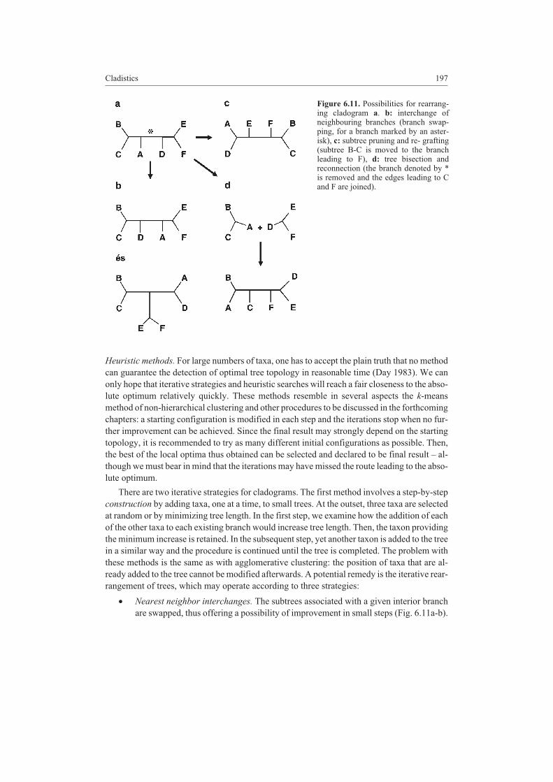
� Nearest neighbor interchanges. The subtrees associated with a given interior branch

are swapped, thus offering a possibility of improvement in small steps (Fig. 6.11a-b).

Cladistics 197

Figure 6.11. Possibilities for rearrang-ing cladogram a. b: interchange ofneighbouring branches (branch swap-ping, for a branch marked by an aster-isk), c: subtree pruning and re- grafting(subtree B-C is moved to the branchleading to F), d: tree bisection andreconnection (the branch denoted by *is removed and the edges leading to Cand F are joined).

Every such branch has four subtrees with three different possible rearrangements.

Thus, the number of new possibilities to be examined is two for each branch.

� Subtree pruning and regrafting. It is examined whether the relocation of subtrees to

different positions in the tree improves tree length (such a relocation is shown in Fig-

ure 6.11c). In each step, the subtree giving the maximum decrease of tree length is

pruned and regrafted.

� Bisection and reconnection. The tree is cut into two subtrees at every possible loca-

tion, the branch bisected is removed and the resulting subtrees are reconnected in all

possible ways (e.g., Fig. 6.11d). Of the new configurations the most optimal is re-

tained. The latter two operations may provide drastic improvements of tree length in a

single step, whilst the majority of relocations are just much worse than the starting to-

pology.

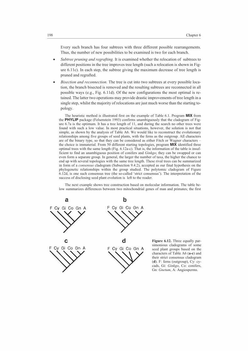
The heuristic method is illustrated first on the example of Table 6.1. Program MIX fromthe PHYLIP package (Felsenstein 1993) confirms unambiguously that the cladogram of Fig-ure 6.7a is the optimum. It has a tree length of 11, and during the search no other trees werefound with such a low value. In most practical situations, however, the solution is not thatsimple, as shown by the analysis of Table A6. We would like to reconstruct the evolutionaryrelationships among five groups of seed plants, with the ferns as the outgroup. All charactersare of the binary type, so that they can be considered as either Fitch or Wagner characters –the choice is immaterial. From 50 different starting topologies, program MIX identified threeoptimal trees with the same length (Fig. 6.12a-c). That is, the information of the table is insuf-ficient to find an unambiguous position of conifers and Ginkgo; they can be swapped or caneven form a separate group. In general, the larger the number of taxa, the higher the chance toend up with several topologies with the same tree length. These rival trees can be summarizedin form of a consensus cladogram (Subsection 9.4.2), accepted as our final hypothesis on thephylogenetic relationships within the group studied. The polytomic cladogram of Figure6.12d, is one such consensus tree (the so-called ‘strict consensus’). The interpretation of thesuccess of disclosing seed plant evolution is left to the reader.

The next example shows tree construction based on molecular information. The table be-low summarizes differences between two mitochondrial genes of man and primates; the first

198 Chapter 6

Figure 6.12. Three equally par-simonious cladograms of someseed plant groups based on thecharacters of Table A6 (a-c) andtheir strict consensus cladogram(d). F: ferns (outgroup), Cy: cy-cads, Gi: Ginkgo, Co: conifers,Gn: Gnetum, A: Angiosperms.

five columns refer to the tRNA of LEU, the others to the tRNA of SER (data from Brown etal. 1982). The total length of these two RNA segments is 131 nucleotides. In the majority ofpositions, the sequences are identical, and these positions are omitted from the table sincethey do not influence the result. Numbering of the positions is therefore arbitrary. (Note thatthe gap detected for the orangutan does not contribute to tree length.) The sequences are givenby

Positions

1 2 3 4 5 6 7 8 9 10 11 12 13 14 15 16 17 18 19

Man A T A C C T A C A C A T G C C C A T C

Chimpanzee A C G C C T A T A T A T A T C C A C C

Gorilla A T A A C T G T G C A T A C C C G C T

Orangutan G T C A T T A C A C T C A C T . A T G

Gibbon A T A A C C A C A C A C T A T C A T A

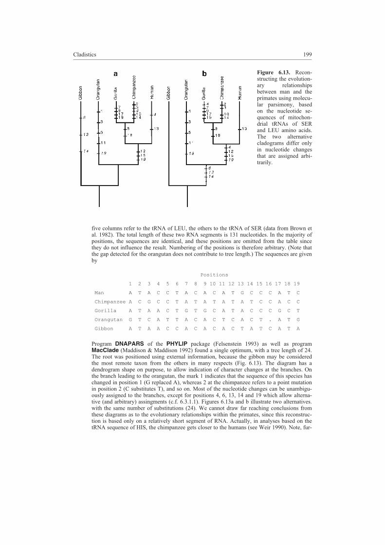
Program DNAPARS of the PHYLIP package (Felsenstein 1993) as well as programMacClade (Maddison & Maddison 1992) found a single optimum, with a tree length of 24.The root was positioned using external information, because the gibbon may be consideredthe most remote taxon from the others in many respects (Fig. 6.13). The diagram has adendrogram shape on purpose, to allow indication of character changes at the branches. Onthe branch leading to the orangutan, the mark 1 indicates that the sequence of this species haschanged in position 1 (G replaced A), whereas 2 at the chimpanzee refers to a point mutationin position 2 (C substitutes T), and so on. Most of the nucleotide changes can be unambigu-ously assigned to the branches, except for positions 4, 6, 13, 14 and 19 which allow alterna-tive (and arbitrary) assingments (c.f. 6.3.1.1). Figures 6.13a and b illustrate two alternatives.with the same number of substitutions (24). We cannot draw far reaching conclusions fromthese diagrams as to the evolutionary relationships within the primates, since this reconstruc-tion is based only on a relatively short segment of RNA. Actually, in analyses based on thetRNA sequence of HIS, the chimpanzee gets closer to the humans (see Weir 1990). Note, fur-

Cladistics 199

Figure 6.13. Recon-structing the evolution-ary relationshipsbetween man and theprimates using molecu-lar parsimony, basedon the nucleotide se-quences of mitochon-drial tRNAs of SERand LEU amino acids.The two alternativecladograms differ onlyin nucleotide changesthat are assigned arbi-trarily.

ther, that all nucleotide replacements were equally weighted: the transitions (A-G, and C-Tchanges, i.e., purine to purine and pyrimidine to pyrimidine) and transversions (a purine is re-placed by a pyrimidine or vice versa) were not distinguished. In reality, however, even thoughthere are twice as many possibilities for transversions than for transitions, the latter are muchmore frequent for chemical reasons. (In the present example, only 6 of the 24 mutations aretransversions.) This may be compensated for by differential weighting from experimentallyderived transition/transversion ratios (e.g., Williams & Fitch 1990, Williams 1992).

6.3.1.3 Evaluation of cladograms

Character-based cladograms, except for the Dollo type, may be evaluated by simple indices.

Kluge and Farris (1969) proposed, for example, to examine for each character the ratio of the

number of changes to the theoretical minimum that can be achieved for another tree topology.

If, in a given tree, character j suffers a total of sj changes whilst another tree could be derived

from the same data in which the minimum mj changes are sufficient, then the ratio

CIm

sj

j

j

� (6.9)

will measure the consistency of character j (consistency index). CIj equals 1 if the possible

minimum occurs in the tree; that is, there is no homoplasy for character j. Any other value in-

dicates some homoplasy. For instance, the value of CIj = 0.5 corresponds to a situation when

twice as many changes occur in the tree than would be necessary in another tree that is opti-

mum for this character. The index is not defined for constant characters, because of obvious

singularity problems (CI = 0/0).

There is only one character, nucleotide position 4, on the cladogram of Figure 6.13 forwhich the consistency index is lower than 1 (CI4 = 0.5). The cladogram of Fig. 6.13a suggeststhat A was replaced by C in man and chimpanzee independently, whereas the tree of Fig.6.13b implies that A (the ancestral state) appeared again in gorilla as a reversal, because in themeantime there was a substitution to C in that position. (Both cases are plausible, showingthat arbitrary choices may lead to different explanations of the same tree.) Position 4 wouldshow a single change, if gibbon, orangutan and gorilla were on the same branch, whereaschimpanzee and man were on another. This is not the case, so two steps were necessary. Thisis of course a mere illustration of the index, because for sequence data reversals and paralleloccurrences are not as unlikely as for morphological characters; in fact, homoplasy is verynatural for RNA and DNA data

The mean consistency index is calculated for all characters:

CI m sj

n

j

j

n

j( )� �� �

� �1 1

(6.10)

which, in our example, takes the value of 0.96 (position 16 was omitted because of the gap).Maddison & Maddison (1992) recommend omission of all autapomorphies as well, becausetheir consistency index is inevitably 1. Therefore, their inclusion in the overall measure wouldinvolve gross distortion if there are many autapomorphic characters in the data.

The retention index (Farris 1989), denoted by Mj for character j, also considers the maximum

of possible changes,

RIM s

M mj

j j

j j

��

�. (6.11)

200 Chapter 6

The lower the contribution of homoplasy to synapomorphies, the greater the value of this in-

dex. If there is no homoplasy at all, then RIj = 1, whereas RIj = 0 results if all synapomorphies

are caused by homoplasy. We would have a 0/0 contribution by apomorphic characters, so

they are excluded from the calculations. The retention index is meaningful only in cases with

some probability of homoplasy, that is, when the minimum and the maximum are unequal (the

denominator is nonzero).

For the RNA example, five positions may be used for calculating RI. Position 4 takes thepossible maximum of two changes, and therefore RI4 = (2–2) / (2–1) = 0. For positions 8, 12,15 and 18, there could have been homoplasy also, but the tree depicts real synapomorphies sothat RIj = (2–1) / (2–1) = 1 for all.

The ensemble retention index is also confined to characters for which Mj > mj:

RI

M s

M m

j

n

j j

j

n

j j

( )� �

�

�

�

�

�

�

1

1

. (6.12)

Its interpretation is the same as that of the character-wise index. For the cladogram of Figure6.13, the RI(�) measure yields 4/5 = 0.8.

6.3.2 Evaluation of character compatibility

An alternative to character-based cladistics is compatibility analysis developed by LeQuesne

(1969, 1972), Estabrook et al. (1976) and others. The objective is the same in both approaches;

the difference is that compatibility analysis discards all characters that lead to homoplasy

(‘false’ characters). Those not conflicting with one another are termed the compatible charac-

ters and only these are retained for further analysis. The central part of the algorithm is to find

the largest possible subset of such characters to yield an unambiguous basis for tree construc-

tion.

The method is illustrated by a simple example. Assume that characters A and B are to be

evaluated for compatibility. Both of them have two states: 0 stands for the ancestral and 1 for

the derived state. The primitive taxon, i.e., the common ancestor of the group had the combi-

nation (0,0) for these characters. Let us say that character A evolved first into the state of 1,

leading to the appearance of combination (1,0). Later, the other character was also changed,

causing a move from the ancestral combination (0,0) into (0,1), or from the more recent (1,0)

combination into (1,1) (Figure 6.14a-b). The simultaneous appearance of combinations (1,1)

and (0,1) in the tree can only be explained by homoplasy: (i) the state 1 for character B was in-

dependently derived twice (parallel evolution, Fig. 6.14c) or (ii) there was a reversal for char-

acter A (Fig. 6.14d). If homoplasy does not occur, then we may find either (0,1) or (1,1)

among the taxa studied. In general, of the four combinations of two characters only three may

appear in the group. Whenever all combinations are detected, the two characters in question

are deemed to be incompatible. This evaluation is performed for each pair of characters and

the results are summarized in a compatibility graph (Fig. 6.14e). In this, the nodes represent

characters, and two nodes are connected by an edge if the associated characters are compatible

with each other. Then, the largest complete subgraph (or ‘clique’) is found. In a clique, all

points are connected with the others, representing the largest subset of characters that can be

Cladistics 201

used unambiguously for tree reconstruction (B, C and D in Figure 6.14e). Of course,

autapomorphic characters may be exluded from such comparisons, because they cannot have

four combinations anyway with any other character in the data. These are members of all

cliques, and can be used later to explain patristic changes on the terminal branches of the tree.

Evaluation of pairwise character compatibility can easily lead to the conclusion that most

of the characters have to be excluded from phylogenetic reconstruction; in sharp contrast with

parsimony methods. This is the strongest argument expressed by many taxonomists against

the use of cliques in cladistics. Meacham & Estabrook (1985) have found that, on the average,

50% of characters were discarded in studies published to date. Occasionally, as many as 90%

had to be omitted! Further difficulty is that only binary (two-state) characters can be used, and

the resulting tree is usually polytomic. Notwithstanding the sound theoretical foundations, the

number of applications of compatibility analysis is therefore negligible as compared to parsi-

mony studies. Thus, further details of the procedure can be omitted here. Interested readers

may consult Mayr & Ashlock (1991: 307-313) for complete algorithmic details.

6.4 Other possibilities for evaluating nucleotide sequences – in brief

We have seen above that both the distance- and the character-based approaches are suitable to

nucleotide sequences – and the possibilities are not yet exhausted. For the sake of complete-

ness, two additional methods will be discussed here, even though they do not fit very well the

main topics of this book. In these, emphasis will be shifted from topology optimization to-

wards a genetically more meaningful interpretation of substitutions and their statistical mod-

eling.

202 Chapter 6

Figure 6.14. Two binary charactersare compatible with each other if nomore than three combinations oftheir states appear in the group oftaxa studied (a-b), because the oc-currence of the fourth can only beexplained by homoplasy (c-d).Characters suitable to cladisticanalysis are identified by findingthe maximally connected subgraphof the compatibility graph (e: B, C,D).

6.4.1 The method of invariants

The importance of the transition/transversion ratio was already mentioned at the end of Sub-

section 6.3.1.2, on the example of short mtRNA sequences of primates. Whereas most parsi-

mony methods do not make distinction between transitions and transversions11

, the method of

invariants proposed by Lake (1987) considers transversions only. Four sequences can be ana-

lyzed at a time, and only those positions are viewed in which two sequences have pu-

rine-based and the other two have pyrimidine-based nucleotides. Transversions on the

terminal branches of the tree are emphasized greatly. The three possible unrooted trees for

four sequences are evaluated for each appropriate nucleotide position, and the optimum is se-

lected using a special scoring system. Although the method will not be described completely,

some details of counting are worth illustrating. Suppose that taxa 1 and 2 are neighbours to

each other, and so are taxa 3 and 4 in the tree being evaluated. If the first two taxa have identi-

cal purine nucleotides whilst the other two taxa have identical pyrimidine nucleotides, then

this position supports the given tree (Fig. 6.15a). Now the common ancestry of taxa 1 and 2 is

very likely, because for any other topology we must assume two transversions of the same

type which, needless to say, is much less probable. (It is still possible though, but some error is

always unavoidable.) The situation is similar if sequences 1 and 2 have different purines and,

at the same time, sequences 3 and 4 possess different pyrimidines, because in this case the to-

pology can be entirely explained by transitions on the terminal branches (Fig. 6.15b). If the

first two sequences have different purines whereas the other two have identical pyrimidines,

then this nucleotide position is contradictory with tree topology. It is because the given tree as-

sumes two parallel, yet different transversions (Fig. 6.15c). By the same token, the opposite

situation (Fig. 6.15d) also counts negatively. After the summation of positive and negative

‘votes’ we may identify the topology supported by the majority of nucleotide positions. A se-

rious disadvantage of the method is that no algorithm is available for more than four se-

quences (Swofford & Olsen 1990:474).

Cladistics 203

Figure 6.15. Lake’s method to de-cide whether a given nucleotideposition supports (a-b) or rejects(c-d) a given evolutionary tree forsequences 1-4.

11 Of course, transitions can be simply forgotten in a parsimony study. Contrary to ‘global parsimony’, the method

of ‘transversion parsimony’ relies exclusively upon transversions (e.g., Cracraft & Helm-Bychowski 1990).

6.4.2 The maximum-likelihood method

The application of this procedure requires some meaningful model of molecular evolution:

the phylogenetic pattern is disclosed on the basis of strict assumptions on the possible trans-

formations of one sequence into another (for morphological data, no such general models are

plausible). The maximum likelihood method will select the most probable tree, under the as-

sumptions specified by the modeler. The modification of tree topology is not part of the

model, for this purpose we can use any of the techniques described in Subsection 6.3.1.2. The

simplest is the Jukes & Cantor model (Felsenstein 1981) in which the four nucleotides have

the same frequency in the sample of sequences and all substitutions are considered equally

likely. The two-parameter model proposed by Kimura (1980) introduces the k transi-

tion/transversion ratio, thus making distinction between the two main types of substitutions.

Its generalized version allows inequal nucleotide frequencies as well (Kishino & Hasegawa

1989). During computations, all positions are taken into account, in contrast with the parsi-

mony methods which do not bother with invariant positions. The heart of the model is a 4�4

matrix determined from the k values and nucleotide frequencies. Each entry in this matrix is

the substitution rate for two nucleotides per unit time. Based on this information, the probabil-

ity that, say, nucleotide A is replaced by G after time t is calculated (see Swofford & Olsen

1990:477-478, for details). Let this probability be denoted by PAG(t). The L likelihood that in a

given position of the sequence we have A which will then be replaced by G after time t is ob-

tained as

L t f P tAG A AG( ) ( )� , (6.13)

where fA is the relative frequency of nucleotide A in the starting sequence. If, for the sake of

simplicity, we assume that the substitions may happen independently on every position during

evolution (which is not so, cf. Weir 1990), then the likelihood that after time t sequence X will

evolve into sequence Y is derived from the likelihood function given by

L t f P tXY

i

s

x x yi i i( ) ( ),�

��

1

, (6.14)

where s is the length of the two sequences (that is, they are of the same length or, more pre-

cisely, the model ignores deletions), xi and yi stand for the nucleotides (A, G, C or T(U)) oc-

curring in position i of sequences X and Y, respectively. Since this is a very small number, the

transformation ln LXY(t) will greatly simplify the calculations.

Function 6.13 is in fact the similarity of molecules X and Y; the higher the likelihood the

closer are the two sequences. The ‘only’ question remaining is how to determine the likeli-

hood for the entire cladogram with more than two sequences! Without entering into the details

of the fairly complex algorithm, it is noted that the tree is built up step by step, one taxon added

at a time to a subtree. The likelihood of the transition is calculated for all positions based on

the existing subtree, and then the last product will provide the likelihood of the entire tree. The

objective is to find a graph for which this quantity is the maximum. This tree depicts the most

likely pathways of evolution, provided that the starting assumptions of the model were cor-

rect. The determination of interior nodes and the details of the calculations are described, for

example, by Felsenstein (1981), Weir (1990:276-286) and Swofford & Olsen (1990:

204 Chapter 6

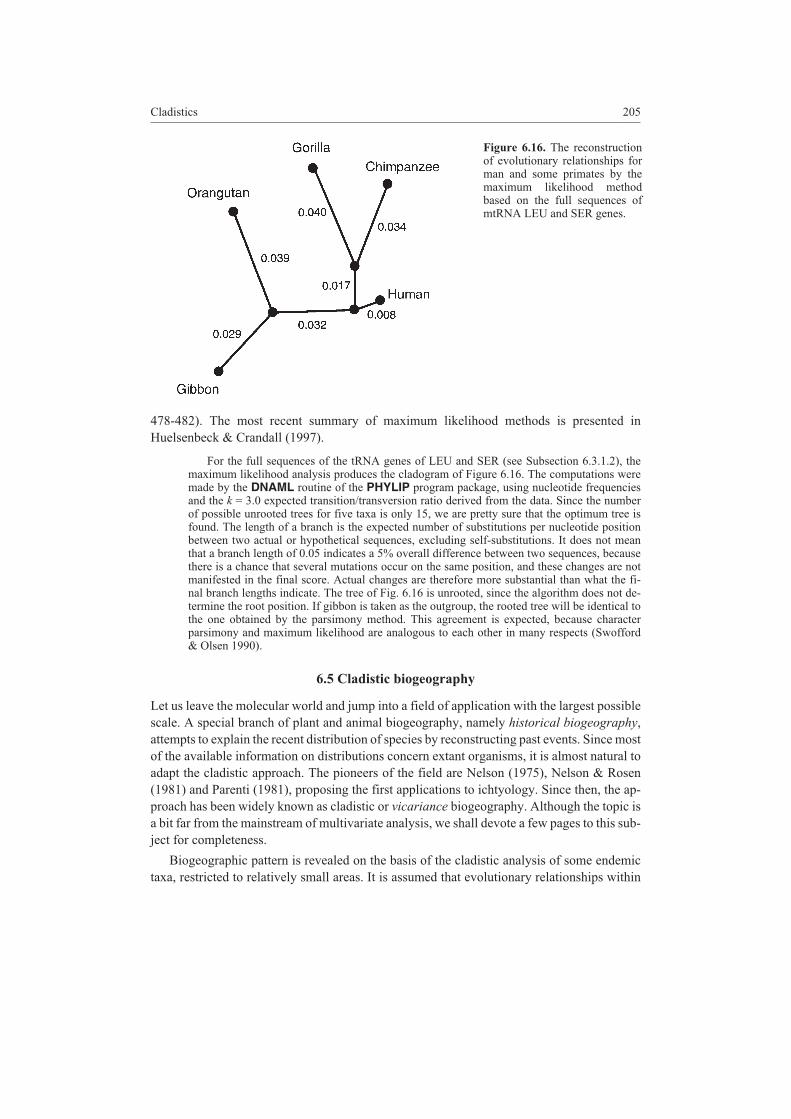
478-482). The most recent summary of maximum likelihood methods is presented in

Huelsenbeck & Crandall (1997).

For the full sequences of the tRNA genes of LEU and SER (see Subsection 6.3.1.2), themaximum likelihood analysis produces the cladogram of Figure 6.16. The computations weremade by the DNAML routine of the PHYLIP program package, using nucleotide frequenciesand the k = 3.0 expected transition/transversion ratio derived from the data. Since the numberof possible unrooted trees for five taxa is only 15, we are pretty sure that the optimum tree isfound. The length of a branch is the expected number of substitutions per nucleotide positionbetween two actual or hypothetical sequences, excluding self-substitutions. It does not meanthat a branch length of 0.05 indicates a 5% overall difference between two sequences, becausethere is a chance that several mutations occur on the same position, and these changes are notmanifested in the final score. Actual changes are therefore more substantial than what the fi-nal branch lengths indicate. The tree of Fig. 6.16 is unrooted, since the algorithm does not de-termine the root position. If gibbon is taken as the outgroup, the rooted tree will be identical tothe one obtained by the parsimony method. This agreement is expected, because characterparsimony and maximum likelihood are analogous to each other in many respects (Swofford& Olsen 1990).

6.5 Cladistic biogeography

Let us leave the molecular world and jump into a field of application with the largest possible

scale. A special branch of plant and animal biogeography, namely historical biogeography,

attempts to explain the recent distribution of species by reconstructing past events. Since most

of the available information on distributions concern extant organisms, it is almost natural to

adapt the cladistic approach. The pioneers of the field are Nelson (1975), Nelson & Rosen

(1981) and Parenti (1981), proposing the first applications to ichtyology. Since then, the ap-

proach has been widely known as cladistic or vicariance biogeography. Although the topic is

a bit far from the mainstream of multivariate analysis, we shall devote a few pages to this sub-

ject for completeness.

Biogeographic pattern is revealed on the basis of the cladistic analysis of some endemic

taxa, restricted to relatively small areas. It is assumed that evolutionary relationships within

Cladistics 205

Figure 6.16. The reconstructionof evolutionary relationships forman and some primates by themaximum likelihood methodbased on the full sequences ofmtRNA LEU and SER genes.

the taxa carry information on the relationships among areas as well. It seems fairly logical to

assume that two closely related taxa have similar distributional patterns, whereas more sub-

stantial taxonomic differences indicate greater biogeographic differences. This holds true if

vicariance is considered the only possible explanation of all differences, as opposed to migra-

tion. In other words, the common ancestor is hypothesized to be present all over the area be-

fore speciation began, the species evolved locally without significant migration. This is

obviously not true generally, showing the limitations of cladistic biogeography right away.

The essence of the method is that in the cladogram of two or more monophyletic groups the

taxon names are replaced by their areas, and the comparison of the area-cladograms thus ob-

tained will provide hypotheses on biogeographic relationships. The taxon cladograms are

generated by any of the methods described above; what is new methodologically is the evalua-

tion of alternative cladograms. The alternative area-cladograms are rarely congruent per-

fectly; the past of different taxonomic groups does not necessarily coincide with similar

biogeographic histories. Migration of some taxa and extinction are just two possibilities to ex-

plain the discrepancies.

Rosen’s (1978) method emphasizes the agreements among alternative area-cladograms,

which often leads to omissions (‘reduced area cladograms’). For example, consider the

cladograms of two groups of Figure 6.17 in which area codes are shown on top of the taxon

names. The group formed by taxa a-f informs us on all the five areas, but none of the taxa of

the other group appears in area C, so it is omitted. For area E, the two cladograms suggest con-

trasting interpretations, and it is also discarded. What remains is the fairly strong congruence

with respect to areas A, B and D, summarized by the reduced consensus cladogram of Fig.

6.17c: regions A and B have very similar biogeographic past, whereas region D has a more

different history. The consensus principle is thus an integral part of the method of cladistic

biogeography, even in its simplest form (for details on consensus, see Chapter 9).

For more than two area cladograms, with possible differences or even contradictions as in

Fig. 6.17, the hidden information may be extracted by the method proposed by Nelson &

Platnick (1981). Its advantage is that omissions are unnecessary, even though incomplete

biogeographic information does affect the final cladogram. The subtrees of the area

cladogram are called the components, and the method is known as component analysis, which

should not be confused with principal components analysis to be discussed in Chapter 7. The

components are determined and numbered for each cladogram, and then their comparative

evaluation provides the desired result. The identification of components involves the follow-

ing basic types:

206 Chapter 6

Figure 6.17. Rosen’s reducedarea cladogram (c) as a possi-ble consensus of two startingcladograms (a-b).

� Every area corresponds with a single taxon in the given group. This is the most

straightforward situation, true of components 1 to 3 in the cladogram of Fig. 6.18a

(component 1 is trivial).

� The number of taxa is smaller than that of the areas. Therefore, the position of missing

areas in the cladogram is unknown, thus allowing several alternatives (three are

shown in Fig. 6.18b). These may support existing components 2-3 or produce new

components.

Cladistics 207

Figure 6.18. Identification of components on different types of area cladograms (a-e). f: The synthesisof area cladograms using all components produces a trivial polytomic tree. g: A consensus of areacladograms considering components 2, 3, 4 and 10 only.

� The number of areas exceeds the number of taxa. The redundant information may

now be condensed into a small tree in which components are easily identified (Fig.

6.18c). In the example, the new component 7 emerges.

� One or more taxa are distributed in several areas, so that the area cladogram is unre-

solved. In this case, Nelson & Platnick (1981) suggest the hypothesis that either 1) the

widely distributed species was present everywhere formerly, and then became extinct

locally, so that unresolved areas have a monophyletic or paraphyletic relationship (as

seen in Fig. 6.18d) or 2) the cladogram is informative on only one area and not so on

the others, because migration occurred. In cladistic terminology, it means that unre-

solved areas may have a polyphyletic origin (as exemplified by the cladograms of Fig.

6.18e, in which the position of A is uncertain).

The resulting components thus depend upon our choice between these two hypotheses con-

cerning the widely distributed taxa. The list will almost always contain contradictory compo-

nents (Fig. 6.18 illustrates this on purpose). If one wishes to consider all components, then

there is a chance to get a trivial polytomic consensus cladogram (Fig. 6.18f), which is not a

real advancement compared to Rosen’s reduced area cladograms – even though all areas are

included. A possible remedy of the problem of trivial consensus trees is that some of the com-

ponents are deemed to be ‘false’ and discarded, and the remaining ones serve as a basis for

cladogram construction. (For example, the partially dichotomous cladogram obtained for

components 2, 3, 4 and 10 in Fig. 6.18g.)

The above method includes some subjective elements, but Brooks (1981) suggests a trickto circumvent the problem of arbitrariness. Each component can be expressed in terms of a bi-nary data vector (xij = 1 if area j is included in component i, xij = 0, otherwise). These vec-tors are summarized in a taxon � component data matrix examined in turn by the usualcharacter-based parsimony methods (cf. Humphries et al. 1988). The most parsimoniouscladogram thus obtained appears to be free from the problem of consensus seeking. This isnot entirely true, however, because it implies a change from Tweedledum to Tweedledee: par-simony analysis may very well provide several equally parsimonious cladograms, calling forconsensus approaches again.

6.6 Literature review

The rich literature of cladistics is hard to follow in some places, especially for the novice. Thesituation is best characterized by Hull’s (1984) sarcastic commentary by which the author ad-mits that he would not recommend Hennig’s (1966) book for anyone as an introduction to theprinciples of cladistics. True enough, even the entomologists are strongly advised to begin withsome more didactic texts, leaving the job of interpreting Hennig, the entomologist’s book to his-torians. For zoologists, Mayr & Ashlock (1991) whereas for botanists Stuessy (1990) can berecommended as a good start. Forey et al. (1992) declare explicitly their book as a material foran introductory semester. This book covers practically all major areas of cladistics, from DNAsequence analysis to cladistic biogeography. Quicke (1993) can also be recommended onsimilar grounds; the principles of cladistics are embedded in a general discussion of taxonomicmethodology. The rapid development of molecular cladistics can be best understood fromSwofford & Olsen (1990), Nei (1996), Li (1997) and Page and Holmes (1998). Be warned thatthe literature of cladistic methodology becomes obsolete very quickly, and it is not worth con-sulting too old books and articles, unless someone wishes to get a deep insight into the history

208 Chapter 6

of some particular subject. Changes, trends and recent developments in this field can be besttraced from periodicals. The cladistic approach has its own forum called, not surprisingly, theCladistics, but this is not the only one to be monitored in the biological literature. Journals suchas Systematic Biology (formerly Systematic Zoology), Systematic Botany, Taxon and Plant

Systematics and Evolution are also important sources of information. Recent advances inbiogeography are reported in the Journal of Biogeography. Evolution, Molecular Phylogenetics

and Evolution and the Journal of Molecular Evolution are inevitable for molecularphylogenetists, but this list is far from being complete. More recently, almost all taxonomic andgenetic journals have published cladistic results, illustrating the increasing importance (andpopularity) of the topic. (Zander [1998] points out that in 1997 75% of the NSF systematics re-search grants in the USA was awarded to modern computerized evolutionary surveys.) Also,there are several good collections of selected papers (e.g., Duncan & Stuessy 1985) and con-ference proceedings (Duncan & Stuessy 1984, Funk & Brooks 1981), to name only a few.

6.6.1 Computer programs

The market of cladistic packages has been dominated by four programs, because of the exper-tise behind and that they provide the widest selection of options. Table 6.2 summarizes theavailability of methods discussed in this book. For a more exhaustive, although older compari-son, see Sanderson (1990).

Note that MacClade (Maddison & Maddison 1992) is a Macintosh application. It is veryeasy to use, and the graphical and printing capabilities are excellent (some of the figures in thischapter were made by this program). MacClade is particularly useful for tracing character evo-lution (the change of a single character along the tree), which is useful for both molecular andmorphology-based cladistics. Admittedly, it is less efficient in finding most parsimonious trees.

Cladistics 209

Table 6.2. Some selected options in the four most widely known cladistic packages (the list is not ex-haustive since other techniques, such as bootstrap and consensus, also appear in these programs).

Method PHYLIP PAUP HENNIG MacClade

Saitou - Nei’s neighbor joining ++

Fitch - Margoliash ++

Wagner distance ++

Parsimony for unordered characters ++ ++ ++ ++

Wagner parsimony ++ ++ ++ ++

Dollo parsimony ++ ++ ++

Stratigraphic parsimony ++

Camin-Sokal parsimony ++

“Branch and bound” ++ ++ ++

Invariants ++ ++

Maximum likelihood ++

Character compatibility ++

The PHYLIP program package (Felsenstein 1993) offers a good choice of options and isfree (including the source code, see Appendix B). Arguments against its use include the rela-tively slow computing speed (Sanderson 1990), alhough the WIN95 version is a good re-sponse to this criticism. Most authors share the view that the best parsimony programs arePAUP (Swofford 1990, new version still unpublished in final form) and HENNIG (Farris 1988).

Many, more specialized programs are omitted from the table. For compatibility analysis, the

CLINCH program (K. Fiala) is best suited, whereas the leading software of cladistic

biogeography is COMPONENT (Page 1989). Felsenstein (1993) lists many more programs in

the documentation of PHYLIP (e.g., Lake’s program for the method of invariants), with informa-

tion on availability and license fees. Nevertheless, the number of programs offered for cladistic

analysis is steadily increasing (see Appendix B, for more information).

6.7 Imaginary dialogue

Q: By reaching the end of this chapter, I really do not see why would the cladists be so conten-

tious, as Gould puts it. No question that they have a fairly rich methodological arsenal, but

this is exactly the case in other fields, as far as I can see it now. The dilemma of choosing

among methods cannot be the bone of discord by itself.

A: True, the technical details are disputed with pretty much the same activity and enthusiasm

as elsewhere in mathematical biology. In the frame of a single and short chapter, I had no

space to go far beyond the issues of plain methodology. The biological and, in particular, the

philosophical aspects of cladism were just touched, but these are the real subjects of contro-

versies! For example, the transformed cladists (‘pattern cladists’) assert that application of the

cladistic methodology does not necessarily imply any reference to evolution. For them, espe-

cially the founders of cladistic biogeography (Nelson, Platnick and Rosen) cladistics is a tool

of revealing a dichotomous hierarchical pattern among the objects, whatever they are. Even

though none of them denied explicitly the evidence of evolution at all, their views led to seri-

ous consequences outside biology, because many creationists misinterpreted the philosophy

of their approach. As a further reading, I can recommend the popular book by Gould (1983)

and the 10th chapter in Dawkins (1986).

Q: I think there is much more to say, for example, about the relationship of cladistics and bio-

logical classification, a topic just mentioned at the end of Section 6.1.

A: Yes, this is a problem that attracts both cladistic and traditional taxonomists. The principal

question is whether the cladograms are suitable constructs to establish formal classifications

of organisms. If a parsimony analysis produces a comb-like (or chained) tree such as the one

shown in Fig. 6.19a, then all taxonomists would decline to say that “OK, this is the optimum

or even the true branching pattern but then, how do you define high-level taxa? You cannot

think seriously that we shall use as many taxonomic ranks as the number of different hierar-

chical levels implied by the tree. We would get lost in the jungle of sub-subfamilies,

super-superorders and the like.” Even though the topology is well-balanced, the taxonomic

ositions implied by the clades may be ambiguous in a classificatory context. Any single ter -

minal branch can have several autapomorphies, possibly more than the sum of such changes

on several sister branches (Fig. 6.19b). ‘True’ cladists are little interested in the development

of autapomorphic characters, however, because the branching pattern is unaffected by such

210 Chapter 6

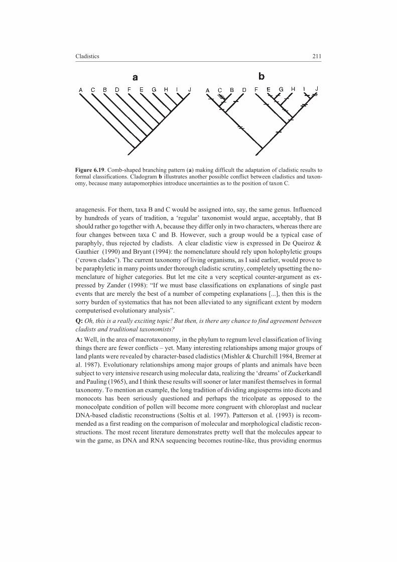
anagenesis. For them, taxa B and C would be assigned into, say, the same genus. Influenced

by hundreds of years of tradition, a ‘regular’ taxonomist would argue, acceptably, that B

should rather go together with A, because they differ only in two characters, whereas there are

four changes between taxa C and B. However, such a group would be a typical case of

paraphyly, thus rejected by cladists. A clear cladistic view is expressed in De Queiroz &

Gauthier (1990) and Bryant (1994): the nomenclature should rely upon holophyletic groups

(‘crown clades’). The current taxonomy of living organisms, as I said earlier, would prove to

be paraphyletic in many points under thorough cladistic scrutiny, completely upsetting the no-

menclature of higher categories. But let me cite a very sceptical counter-argument as ex-

pressed by Zander (1998): “If we must base classifications on explanations of single past

events that are merely the best of a number of competing explanations [...], then this is the

sorry burden of systematics that has not been alleviated to any significant extent by modern

computerised evolutionary analysis”.

Q: Oh, this is a really exciting topic! But then, is there any chance to find agreement between

cladists and traditional taxonomists?

A: Well, in the area of macrotaxonomy, in the phylum to regnum level classification of living

things there are fewer conflicts – yet. Many interesting relationships among major groups of

land plants were revealed by character-based cladistics (Mishler & Churchill 1984, Bremer at

al. 1987). Evolutionary relationships among major groups of plants and animals have been

subject to very intensive research using molecular data, realizing the ‘dreams’ of Zuckerkandl

and Pauling (1965), and I think these results will sooner or later manifest themselves in formal

taxonomy. To mention an example, the long tradition of dividing angiosperms into dicots and

monocots has been seriously questioned and perhaps the tricolpate as opposed to the

monocolpate condition of pollen will become more congruent with chloroplast and nuclear

DNA-based cladistic reconstructions (Soltis et al. 1997). Patterson et al. (1993) is recom-

mended as a first reading on the comparison of molecular and morphological cladistic recon-

structions. The most recent literature demonstrates pretty well that the molecules appear to

win the game, as DNA and RNA sequencing becomes routine-like, thus providing enormus

Cladistics 211

Figure 6.19. Comb-shaped branching pattern (a) making difficult the adaptation of cladistic results toformal classifications. Cladogram b illustrates another possible conflict between cladistics and taxon-omy, because many autapomorphies introduce uncertainties as to the position of taxon C.

amounts of data for cladistic analysis (for various groups of plants, see Chaw et al. 1997, Hoot

et al. 1999, Stefanovic et al. 1998).

Q: I have learned many things about the evaluation of nucleotide sequences, and now you

mention them again. But, I miss something: why do you neglect the possibility of using

amino-acid sequences, that is, proteins in reconstrucing evolutionary pathways? The basic

set of elements is larger than for DNA or RNA, possibly allowing a more refined cladistic

analysis.

A: I cannot elude this question, of course. Protein sequences appear suitable to cladistic analy-

sis, although the various authors disagree as to the utility of such molecules. Swofford &

Olsen (1990) discuss three major issues related to protein-based tree reconstruction: 1) Mini-

mizing the number of amino-acid replacements in parsimony analysis (in other words, the

amino-acid positions are considered as unordered characters, as in case of nucleotide se-

quences). In this approach, the main problem is that there are different numbers of nucleotide

substitutions behind the amino acid replacements. 2) When the proteins are traced back to

mRNA level, then the number of nucleotide substitutions necessary to transform the

amino-acid sequences into one another can be minimized (cf. Goodman 1981), thus consider-

ing the ‘degenerated’ nature of the genetic code. This suffers from the danger of overempha-

sizing ‘silent’ substitutions, however (note that many substitutions – in position three of the

codons – do not change the amino-acid coded). 3) Program PROTPARS (Felsenstein 1993)

eliminates the problem of silent substitutions, so that this is perhaps the best software for eval-

uating amino-acid sequences. You can see that the proteins are not used by themselves. In-

deed, the genetic code behind them is used most efficiently. Nevertheless, there are clear

arguments in favour of using amino-acid sequences directly in certain cases (Nei 1996): the

comparison of distantly related protein-coding DNA sequences is burdened by several com-

plications (synonymous substitutions, transversion/transition bias, non-stationarity of nucleo-

tide substitutions) so that long term evolution is better revealed by using proteins. There is a

maximum likelihood method for proteins as well (Kishino et al. 1990).

Q: It turned out early that the results of cladistic analysis are as much influenced by the per-

sonal judgment and experience of the investigator, as hierarchical classifications. In the pre-

vious chapter, you emphasized the importance of choosing among different methods and the

necessity of comparisons. I miss the analogous treatment of cladograms, however...

A: Frankly speaking, there was simply no space, time and ‘energy’ for such an expanded dis-

cussion here. In the literature, you find several papers reporting on thorough comparative

studies, such as Duncan et al. (1980) and Astolfi et al. (1981). Extensive evaluations of molec-

ular cladistic techniques are provided by Saitou & Imanishi (1989) and Nei (1991). Different

programs written for the same purpose are also compared sometimes, as done by Luckow &

Pimentel (1985) with Wagner parsimony methods. And you know why: optimizing tre topol-

ogy is an NP-complete problem, so that the success of heuristic search greatly depends on the

computer program you are using.

Q: The maximum likelihood method seems to have the advantage that one can assess how the

result is influenced by changes in the underlying mathematical model of molecular evolution.

Refinement of these models can lead to more reliable reconstructions, I guess. But, as you

write, no such models are available for morphological characters. Is it really true that we

212 Chapter 6

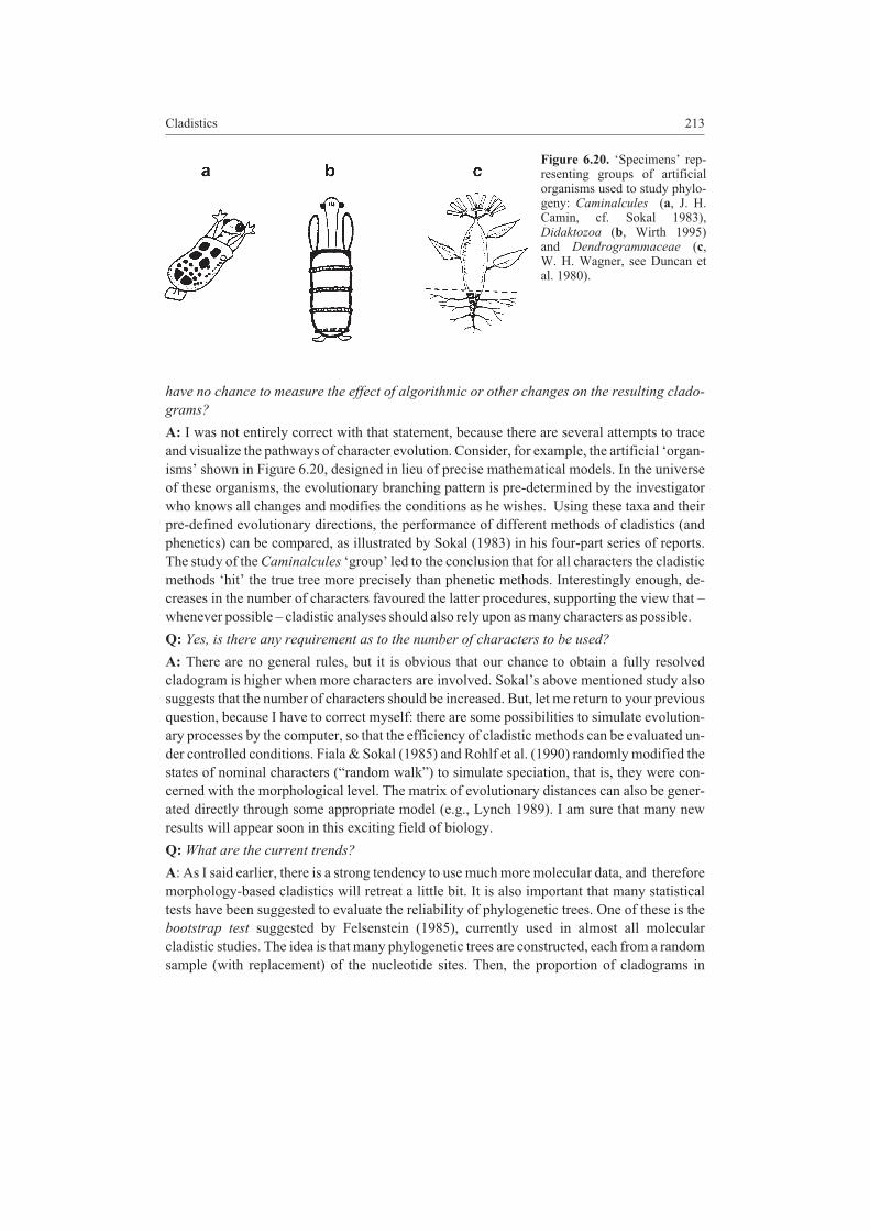
have no chance to measure the effect of algorithmic or other changes on the resulting clado-

grams?

A: I was not entirely correct with that statement, because there are several attempts to trace

and visualize the pathways of character evolution. Consider, for example, the artificial ‘organ-

isms’ shown in Figure 6.20, designed in lieu of precise mathematical models. In the universe

of these organisms, the evolutionary branching pattern is pre-determined by the investigator

who knows all changes and modifies the conditions as he wishes. Using these taxa and their

pre-defined evolutionary directions, the performance of different methods of cladistics (and

phenetics) can be compared, as illustrated by Sokal (1983) in his four-part series of reports.

The study of the Caminalcules ‘group’ led to the conclusion that for all characters the cladistic

methods ‘hit’ the true tree more precisely than phenetic methods. Interestingly enough, de-

creases in the number of characters favoured the latter procedures, supporting the view that –

whenever possible – cladistic analyses should also rely upon as many characters as possible.

Q: Yes, is there any requirement as to the number of characters to be used?

A: There are no general rules, but it is obvious that our chance to obtain a fully resolved

cladogram is higher when more characters are involved. Sokal’s above mentioned study also

suggests that the number of characters should be increased. But, let me return to your previous

question, because I have to correct myself: there are some possibilities to simulate evolution-

ary processes by the computer, so that the efficiency of cladistic methods can be evaluated un-

der controlled conditions. Fiala & Sokal (1985) and Rohlf et al. (1990) randomly modified the

states of nominal characters (“random walk”) to simulate speciation, that is, they were con-

cerned with the morphological level. The matrix of evolutionary distances can also be gener-

ated directly through some appropriate model (e.g., Lynch 1989). I am sure that many new

results will appear soon in this exciting field of biology.

Q: What are the current trends?

A: As I said earlier, there is a strong tendency to use much more molecular data, and therefore

morphology-based cladistics will retreat a little bit. It is also important that many statistical

tests have been suggested to evaluate the reliability of phylogenetic trees. One of these is the

bootstrap test suggested by Felsenstein (1985), currently used in almost all molecular

cladistic studies. The idea is that many phylogenetic trees are constructed, each from a random

sample (with replacement) of the nucleotide sites. Then, the proportion of cladograms in

Cladistics 213

Figure 6.20. ‘Specimens’ rep-resenting groups of artificialorganisms used to study phylo-geny: Caminalcules (a, J. H.Camin, cf. Sokal 1983),Didaktozoa (b, Wirth 1995)and Dendrogrammaceae (c,W. H. Wagner, see Duncan etal. 1980).

which a given clade appears is calculated, indicated at the respective branch in the consensus

cladogram of the alternative trees. For more on recently proposed tests of phylogenetic infer-

ence, you could consult Nei’s (1996) review.

214 Chapter 6