Fluid Mechanics 1

CIVE3086 - Fluid Mechanics

Instructor: Associate Prof. Dr. Ho Viet Hung

Homepage: http://hungtlu.wordpress.com

Chapter 4: Fluid Kinematics

Fluid Mechanics 2

Learning Objectives:

After completing this chapter, you should be able to:

■ discuss the differences between the Eulerian and Lagrangian descriptions of fluid motion.

■ identify various flow characteristics based on the velocity field.

■ determine the streamline pattern and acceleration field given a velocity field.

■ discuss the differences between a system and control volume.

■ apply the Reynolds transport theorem and the material derivative.

Fluid Mechanics 3

Fluid Kinematics

Fluid kinematics is the study of fluid motion without

consideration of the actual force that are causing the

motion.

We will look at the velocity and acceleration of the fluid,

and the description and visualization of its motion.

4.1 The Velocity Field

- Fluid kinematics will be analyzed using continuum

hypothesis (fluids have a molecular structure)

- This allows for the description of fluid flow in term of the

motion of fluid particles.

Fluid Mechanics 4

4.1 The Velocity Field

To describe a fluid flow we must determine the various parameters not

only as a function of the spatial coordinates (x, y, z) but also as a

function of time, t.

Fluid Mechanics 5

- One of the most important fluid variables is the

velocity field.

- We can represent the velocity field as

Where: u, v and w are the x, y, and z components of

the velocity vector.

The velocity of a particle is the time rate of change of

the position vector rA for that particle.

A

A

drV

dt

Fluid Mechanics 6

Fluid Mechanics 7

By writing the velocity for all of the particles we can

obtain the field description of the velocity vector

V = V(x,y,z,t)

Since the velocity is a vector, it has both a direction and

a magnitude. The magnitude of V is the speed of the

fluid.

A change in velocity results in an acceleration. This

acceleration may be due to a change in speed and/or

direction.

dva

dt

Fluid Mechanics 8

4.1.1 Eulerian and Lagrangian Flow

Descriptions

Eulerian method: the fluid motion is described by prescribing the necessary properties (pressure, density, velocity, etc.) as functions of space and time.

• We get information about the flow in terms of what happens at fixed points in space as the fluid flows through those points.

Fluid Mechanics 9

Lagrangian method involves following individual fluid

particles as they move about and determining how the

fluid properties associated with these particles change as

a function of time.

That is, the fluid particles are identified, and their

properties determined as they move.

Fluid Mechanics 10

The difference between the Eulerian and Lagrangian methods: the example of smoke discharging from a chimney.

- In the Eulerian method may

attach a temperature-measuring

device to the top of the chimney

(point 0) and record the

temperature at that point as a

function of time.

- At different times there are

different fluid particles passing by

the stationary device.

- Would obtain the temperature, T,

for that location as a function of

time. ( , , , )o o oT T x y z t

Fluid Mechanics 11

In the Lagrangian method, would attach the temperature-

measuring device to a particular fluid particle (particle A)

and record that particle’s temperature as it moves about.

- Would obtain that particle’s

temperature as a function of time.

- The use of many such

measuring devices moving with

various fluid particles would

provide the temperature of these

fluid particles as a function of

time.

- Lagrangian information can be

derived from the Eulerian data —

and vice versa.

Fluid Mechanics 12

Example 4.1 provides an

Eulerian description of the flow.

For a Lagrangian description

we would need to determine the

velocity as a function of time for

each particle as it flows along

from one point to another.

In fluid mechanics it is usually easier

to use the Eulerian method to

describe a flow—in either

experimental or analytical

investigations.

Fluid Mechanics 13

4.1.2 One-, Two-, and Three-Dimensional Flows

Generally, a fluid flow is a rather complex three-dimensional, time-dependent phenomenon.

The velocity field actually contains all three velocity components (u, y, w).

In many situations the three-dimensional flow characteristics are important. For these situations it is necessary to analyze the flow in its complete three-dimensional character.

Neglect one or two of the velocity components in these cases would lead to considerable misrepresentation of the effects produced by the actual flow.

Fluid Mechanics 14

The flow of air past an airplane wing provides an example

of a complex three-dimensional flow.

Photograph of the flow past a model wing

The flow has been made visible by using a flow visualization technique.

Fluid Mechanics 15

One- and Two- Dimensional Flows

In many situations, one of the velocity components may be small relative to the two other components.

It may be reasonable to neglect the smaller component and assume two-dimensional flow.

where: u and v are functions of x and y (and possibly time, t).

Sometimes possible to further simplify a flow analysis by

assuming that two of the velocity components are

negligible, leaving the velocity field to be approximated as a

one-dimensional flow field.

Fluid Mechanics 16

4.1.3 Steady and Unsteady Flows

Steady flow - the velocity at a given point in space does not vary with time.

Unsteady flows – the velocity does vary with time.

It is not difficult to believe that unsteady flows are usually more difficult to analyze than are steady flows.

Among the various types of unsteady flows are nonperiodic flow, periodic flow, and truly random flow.

0V

t

0V

t

Fluid Mechanics 17

4.1.4 Streamlines and Pathlines

A streamline is a line that is

everywhere tangent to the

velocity field instantaneously.

If the flow is steady, the

streamlines are fixed lines in

space.

For unsteady flows the

streamlines may change shape

with time.

No flow across streamlines.

Fluid Mechanics 18

• For two-dimensional flows the slope of the

streamline must be equal to the tangent of the

angle that the velocity vector makes with the x

axis.

dx dy dz

u v w In general, equation for a streamline:

- Integrate to get streamline equations

Fluid Mechanics 19

A pathline is the

continuous line traced

out by a given particle as

it flows from one point to

another.

The pathline is a

Lagrangian concept that

can be produced in the

laboratory by marking a

fluid particle.dx dy dz

dtu v w Equation for a pathline:

- Integrate to get pathline equations

Fluid Mechanics 20

4.2 The Acceleration Field

We can describe fluid motion by either Lagrangiandescription or Eulerian description.

To apply Newton’s second law we need to describe the particle acceleration in an acceptable manner.

For Lagrangian method, we describe the fluid acceleration just as is done in solid body dynamics, a=a(t) for each particle.

For the Eulerian description we describe the acceleration field as a function of position and time without actually following any particular particle.

We obtain the acceleration field if the velocity field is known.

Fluid Mechanics 21

Consider a fluid particle A moving along its pathline. The

particle’s velocity, VA, is a function of its location and the

time.

Fluid Mechanics 22

We use the chain rule of differentiation to obtain the

acceleration of particle A, denoted aA:

- Which is valid for any particle, we can drop the reference

to particle A and obtain the acceleration field from the

velocity field (this is a vector equation).

Fluid Mechanics 23

Scalar components can be written as follow.

ax, ay, and az are the x, y, and z components of the

acceleration.

Fluid Mechanics 24

In short hand notation, we can write the above result as:

Is called the MATERIAL DERIVATIVE

- The material derivative formula contains two types of

terms: the time derivative (or local derivative)

and spatial derivatives (or convective derivatives).

Fluid Mechanics 25

- Time derivative represents effects of the unsteadiness of

the flow. For steady flow the time derivative is zero.

- Local acceleration

- Convective derivative represents the fact that a flow property may vary because of the motion of the particle from one point in space where the parameter has one value to another point in space where its value is different.

- Convective acceleration terms:

Fluid Mechanics 26

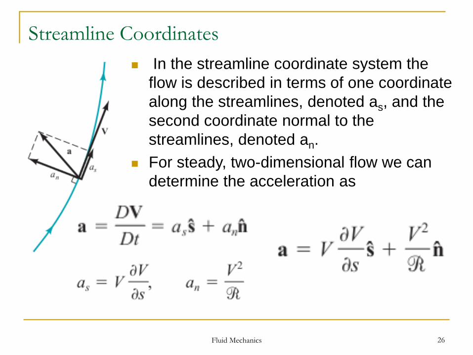
Streamline Coordinates

In the streamline coordinate system the

flow is described in terms of one coordinate

along the streamlines, denoted as, and the

second coordinate normal to the

streamlines, denoted an.

For steady, two-dimensional flow we can

determine the acceleration as

Fluid Mechanics 27

A velocity field is given by:

Determine the streamlines for this flow

(the two-dimensional steady flow).

Example 1

Fluid Mechanics 28

4.3. Control Volume

A control volume is a volume in space (a geometric

entity, independent of mass) through which fluid may

flow.

It can be a moving volume, although for most situations

we will use only fixed, nondeformable control volumes.

• The control volume itself is a

specific geometric entity,

independent of the flowing fluid.

• The amount of mass within the

volume may change with time.

Fluid Mechanics 29

System

A system is a collection of matter of fixed identity (always the same atoms or fluid particles), which may move, flow, and interact with its surroundings.

A system:

- is a specific, identifiable quantity of matter.

- may consist of a relatively large amount of mass, or it may be an infinitesimal size (a single fluid particle).

- It may continually change size and shape, but it always contains the same mass.

Fluid Mechanics 30

System (Sys) and Control Volume (CV)

Fluid Mechanics 31

System and Control Volume

The behavior of a fluid is governed by fundamental

physical laws :

- Conservation of mass,

- Newton’s laws of motion,

- The laws of thermodynamics.

Various ways to apply these governing laws to a fluid

flow, two ways are:

- The system approach,

- The control volume approach.

Fluid Mechanics 32

4.4 The Reynolds Transport Theorem

The Reynolds transport theorem is an analytical tool to

shift from systems representation to an CV

representation.

B represents any of fluid parameters

b represents the amount of that parameter per unit mass.

B = mb

Where: m is the mass of the portion of fluid of interest.

B = mV2/2, the kinetic energy of the mass, then the

b=V2/2, kinetic energy per unit mass.

B = mV, the momentum of the mass, then b = V (the

momentum per unit mass is the velocity).

Fluid Mechanics 33

B = mb

The parameter B is termed an extensive property

The parameter b is termed an intensive property

The value of B is directly proportional to the amount of

the mass being considered,

The value of b is independent of the amount of mass.

Fluid Mechanics 34

Most laws in fluid motion involve the time rate of change of an

extensive property of a fluid system:

- the rate at which the momentum of a system changes with

time,

- OR the rate at which the mass of a system changes with

time.

To formulate the laws into a control volume approach, we

must obtain an expression for the time rate of change

within a control volume.

Fluid Mechanics 35

Fluid flows from the fire extinguisher tank. Discuss the differences between dBsystem/dt and dBcv/dt if B represents mass.

With B=m, the system mass, it follows that b=1

- The time rate of change

of mass within

the system

Example 2: Time Rate of Change for a System

and a Control Volume

- The time rate of change of mass within the

control volume

Fluid Mechanics 36

Choose our system to be the fluid within the tank at the time the valve was opened, and the control volume to be the tank itself.

- A short time after the valve is opened, part of the system has moved outside of the control volume.

- The control volume remains fixed.

- The limits of integration

are fixed for the Control

Volume, but they are

a function of time for the

System.

Fluid Mechanics 37

Example 3:

- Mass conservation implies that:

- Some of the fluid has left the control

volume through the nozzle on the tank:

- For this example,

dBcv /dt < dBsys /dt.

- Other cases may have

dBcv /dt > dBsys /dt.

Fluid Mechanics 38

The Reynolds Transport Theorem

Time rate of change of any arbitrary

parameter B:

Time rate of change of B within CV

as the fluid through the CV:

The net flowrate (or “flux”) of

parameter B across the entire control

surface:

- If b=1 then this term is the mass flow rate (ρAV).

- is the outward normal vector to the surface element.

Fluid Mechanics 39

Inflow and Outflow across the control surface.

- The unit normal vector to the control surface points

out from the control volume.

Inflow (influx): - Outflow (offlux):

Fluid Mechanics 40

Typical control volume with more than one inlet and outlet

Possible velocity configurationson portions of the control surface

Fluid Mechanics 41

Steady Effects

It is a net difference in the rate that B flows into the CV compared with the rate that it flows out of the CV.

The integral of over the inflow portions of the control surface would not be equal and opposite to that over the outflow portions of the surface.

If the parameter B is the mass of the system, the left-hand side of Eq. is zero (conservation of mass for the system).

Assume the parameter B is the momentum of the system. The time rate of change of the system momentum equals the net force acting on the system.

Fluid Mechanics 42

Unsteady Effects

so that all terms in Eq. must be retained.

- For the special unsteady situations in which the rate of

inflow of parameter B is exactly balanced by its rate of

outflow:

Assignment

Homework Assignment #5

Fluid Mechanics 43