City Research Onlineopenaccess.city.ac.uk/13169/1/Castillo-Rivera, Salvador.pdf · Advanced...
320
City, University of London Institutional Repository Citation: Castillo-Rivera, Salvador (2014). Advanced Modelling of Helicopter Nonlinear Dynamics and Aerodynamics. (Unpublished Doctoral thesis, City University London) This is the accepted version of the paper. This version of the publication may differ from the final published version. Permanent repository link: http://openaccess.city.ac.uk/13169/ Link to published version: Copyright and reuse: City Research Online aims to make research outputs of City, University of London available to a wider audience. Copyright and Moral Rights remain with the author(s) and/or copyright holders. URLs from City Research Online may be freely distributed and linked to. City Research Online: http://openaccess.city.ac.uk/ [email protected] City Research Online
Transcript of City Research Onlineopenaccess.city.ac.uk/13169/1/Castillo-Rivera, Salvador.pdf · Advanced...
City, University of London Institutional Repository
Citation: Castillo-Rivera, Salvador (2014). Advanced Modelling of Helicopter Nonlinear Dynamics and Aerodynamics. (Unpublished Doctoral thesis, City University London)
This is the accepted version of the paper.
This version of the publication may differ from the final published version.
Permanent repository link: http://openaccess.city.ac.uk/13169/
Link to published version:
Copyright and reuse: City Research Online aims to make research outputs of City, University of London available to a wider audience. Copyright and Moral Rights remain with the author(s) and/or copyright holders. URLs from City Research Online may be freely distributed and linked to.
City Research Online: http://openaccess.city.ac.uk/ [email protected]
City Research Online
Advanced Modelling of Helicopter
Nonlinear
Dynamics and Aerodynamics
Salvador Castillo-Rivera
Submitted to the City University London
for the degree of
Doctor of Philosophy
School of Engineering and Mathematical Sciences
City University London
December 2014

Contents
I Introduction, Literature Review & VehicleSim Modelling 26
1 Introduction 27
1.1 Thesis Overview . . . . . . . . . . . . . . . . . . . . . . . . . . . . . . . 27
1.2 Motivation and Objectives . . . . . . . . . . . . . . . . . . . . . . . . . . 29
1.3 Thesis Outline . . . . . . . . . . . . . . . . . . . . . . . . . . . . . . . . 30
2 Literature Review 32
2.1 Introduction . . . . . . . . . . . . . . . . . . . . . . . . . . . . . . . . . . 32
2.2 Simulation Approaches . . . . . . . . . . . . . . . . . . . . . . . . . . . . 33
2.3 Main Rotor . . . . . . . . . . . . . . . . . . . . . . . . . . . . . . . . . . 39
2.4 Tail Rotor . . . . . . . . . . . . . . . . . . . . . . . . . . . . . . . . . . . 40
2.5 Fuselage . . . . . . . . . . . . . . . . . . . . . . . . . . . . . . . . . . . . 41
2.6 Equations . . . . . . . . . . . . . . . . . . . . . . . . . . . . . . . . . . . 42
2.7 Stability . . . . . . . . . . . . . . . . . . . . . . . . . . . . . . . . . . . . 45
2.8 Vibrations . . . . . . . . . . . . . . . . . . . . . . . . . . . . . . . . . . . 46
2.9 Aerodynamic Environment . . . . . . . . . . . . . . . . . . . . . . . . . 48
2.10 Unmanned Aerial Vehicles (UAVs) . . . . . . . . . . . . . . . . . . . . . 52
1
CONTENTS
2.11 Chapter Summary . . . . . . . . . . . . . . . . . . . . . . . . . . . . . . 54
3 VehicleSim as Modelling Tool 56
3.1 Introduction . . . . . . . . . . . . . . . . . . . . . . . . . . . . . . . . . . 56
3.2 Overview of VehicleSim Lisp . . . . . . . . . . . . . . . . . . . . . . . . . 56
3.2.1 VehicleSim Lisp . . . . . . . . . . . . . . . . . . . . . . . . . . . . 56
3.2.2 VehicleSim Operation . . . . . . . . . . . . . . . . . . . . . . . . 57
3.2.3 Multibody Modelling . . . . . . . . . . . . . . . . . . . . . . . . . 59
3.3 VehicleSim Characteristics . . . . . . . . . . . . . . . . . . . . . . . . . . 62
3.3.1 State Variables . . . . . . . . . . . . . . . . . . . . . . . . . . . . 62
3.3.2 Equations of Motion . . . . . . . . . . . . . . . . . . . . . . . . . 63
3.3.3 Numerical Solution . . . . . . . . . . . . . . . . . . . . . . . . . . 65
3.4 Building a Model . . . . . . . . . . . . . . . . . . . . . . . . . . . . . . . 69
3.5 Chapter Summary . . . . . . . . . . . . . . . . . . . . . . . . . . . . . . 72
II Helicopter Models 73
4 Caliber 3 Dynamic Model 74
4.1 Introduction . . . . . . . . . . . . . . . . . . . . . . . . . . . . . . . . . . 74
4.2 Caliber 3 Description and Parameters Identification . . . . . . . . . . . 75
4.3 Model Description . . . . . . . . . . . . . . . . . . . . . . . . . . . . . . 78
4.4 Fuselage Modelling . . . . . . . . . . . . . . . . . . . . . . . . . . . . . . 79
4.5 Swashplate and Main Rotor Modelling . . . . . . . . . . . . . . . . . . . 80
4.5.1 Swashplate Modelling . . . . . . . . . . . . . . . . . . . . . . . . 80
4.5.2 Main Rotor Modelling . . . . . . . . . . . . . . . . . . . . . . . . 82
2

CONTENTS
4.5.3 Controllers and Moments Definition . . . . . . . . . . . . . . . . 88
4.6 Tail Rotor Modelling . . . . . . . . . . . . . . . . . . . . . . . . . . . . . 93
4.6.1 Bodies Definition . . . . . . . . . . . . . . . . . . . . . . . . . . . 93
4.6.2 Controllers Implementation . . . . . . . . . . . . . . . . . . . . . 96
4.6.3 Feather Control Definition . . . . . . . . . . . . . . . . . . . . . . 96
4.6.4 Flap Control Definition . . . . . . . . . . . . . . . . . . . . . . . 97
4.7 Simulations and Results . . . . . . . . . . . . . . . . . . . . . . . . . . . 99
4.7.1 Vibrations . . . . . . . . . . . . . . . . . . . . . . . . . . . . . . . 99
4.7.2 Position and Rotation Control . . . . . . . . . . . . . . . . . . . 101
4.8 Chapter Summary . . . . . . . . . . . . . . . . . . . . . . . . . . . . . . 103
5 Sikorsky Configuration Dynamic Model 106
5.1 Introduction . . . . . . . . . . . . . . . . . . . . . . . . . . . . . . . . . . 106
5.2 Model Description . . . . . . . . . . . . . . . . . . . . . . . . . . . . . . 112
5.3 Dynamic Model . . . . . . . . . . . . . . . . . . . . . . . . . . . . . . . . 114
5.4 Fuselage Modelling . . . . . . . . . . . . . . . . . . . . . . . . . . . . . . 116
5.5 Main Rotor Modelling . . . . . . . . . . . . . . . . . . . . . . . . . . . . 118
5.5.1 Bodies Definition . . . . . . . . . . . . . . . . . . . . . . . . . . . 118
5.5.2 Controllers and Moments Definitions . . . . . . . . . . . . . . . . 122
5.6 Tail Rotor Modelling . . . . . . . . . . . . . . . . . . . . . . . . . . . . . 129
5.6.1 Bodies Definition . . . . . . . . . . . . . . . . . . . . . . . . . . . 130
5.6.2 Controllers Implementation . . . . . . . . . . . . . . . . . . . . . 133
5.7 Vehicle’s Longitudinal and Angular Position Control . . . . . . . . . . . 139
5.8 Chapter Summary . . . . . . . . . . . . . . . . . . . . . . . . . . . . . . 141
3
CONTENTS
6 External Perturbations Modelling for Sikorsky Model (Aerodynamic
Model) 143
6.1 Introduction . . . . . . . . . . . . . . . . . . . . . . . . . . . . . . . . . . 143
6.1.1 Aerodynamic Environment . . . . . . . . . . . . . . . . . . . . . 144
6.2 Earth/Ground Modelling . . . . . . . . . . . . . . . . . . . . . . . . . . 152
6.3 Main Rotor Tilt . . . . . . . . . . . . . . . . . . . . . . . . . . . . . . . 153
6.4 Main Rotor Varying Angular Speed . . . . . . . . . . . . . . . . . . . . . 155
6.5 Main Rotor Aerodynamic Modelling . . . . . . . . . . . . . . . . . . . . 156
6.5.1 Air Density . . . . . . . . . . . . . . . . . . . . . . . . . . . . . . 156
6.5.2 Induced Hover Speed . . . . . . . . . . . . . . . . . . . . . . . . . 156
6.5.3 Climb, Descent and Forward Speed . . . . . . . . . . . . . . . . . 157
6.5.4 Induced Climb, Descent and Forward Velocities . . . . . . . . . . 158
6.5.5 Blade Angle of Incidence . . . . . . . . . . . . . . . . . . . . . . 159
6.5.6 Lift Force . . . . . . . . . . . . . . . . . . . . . . . . . . . . . . . 161
6.5.7 Drag Force . . . . . . . . . . . . . . . . . . . . . . . . . . . . . . 163
6.5.8 Thrust Coefficients . . . . . . . . . . . . . . . . . . . . . . . . . . 164
6.5.9 Climb Angle . . . . . . . . . . . . . . . . . . . . . . . . . . . . . 166
6.6 Tail Rotor Aerodynamic Modelling . . . . . . . . . . . . . . . . . . . . . 167
6.6.1 Blade Angle of Incidence for Hover, Climb, Descent and Forward
Flight . . . . . . . . . . . . . . . . . . . . . . . . . . . . . . . . . 167
6.6.2 Tail Rotor Lift Force . . . . . . . . . . . . . . . . . . . . . . . . . 169
6.6.3 Tail Rotor Thrust Coefficient . . . . . . . . . . . . . . . . . . . . 171
6.7 Flight Control . . . . . . . . . . . . . . . . . . . . . . . . . . . . . . . . . 172
6.7.1 Longitudinal Position Control . . . . . . . . . . . . . . . . . . . . 173
4
CONTENTS
6.7.2 Vertical Position Control . . . . . . . . . . . . . . . . . . . . . . 174
6.7.3 Tail Rotor Flap Control . . . . . . . . . . . . . . . . . . . . . . . 177
6.8 Chapter Summary . . . . . . . . . . . . . . . . . . . . . . . . . . . . . . 178
III Results 180
7 Sikorsky Model in Absence of External Perturbations 181
7.1 VehicleSim Equations of Motion . . . . . . . . . . . . . . . . . . . . . . 181
7.1.1 Flap Dynamical Equations . . . . . . . . . . . . . . . . . . . . . 182
7.1.2 Lag Dynamical Equations . . . . . . . . . . . . . . . . . . . . . . 184
7.1.3 Feather Equations of Motion . . . . . . . . . . . . . . . . . . . . 187
7.1.4 Coupled Equations of Flap and Lag . . . . . . . . . . . . . . . . 188
7.2 Dynamical Analysis . . . . . . . . . . . . . . . . . . . . . . . . . . . . . 190
7.2.1 Flap Dynamics . . . . . . . . . . . . . . . . . . . . . . . . . . . . 190
7.2.2 Lag Dynamics . . . . . . . . . . . . . . . . . . . . . . . . . . . . 193
7.2.3 Coupled Flap and Lag Dynamics . . . . . . . . . . . . . . . . . . 194
7.2.4 Frequency Domain Validation . . . . . . . . . . . . . . . . . . . . 197
7.2.5 Feather . . . . . . . . . . . . . . . . . . . . . . . . . . . . . . . . 201
7.2.6 Fuselage . . . . . . . . . . . . . . . . . . . . . . . . . . . . . . . . 202
7.2.7 Tail Rotor . . . . . . . . . . . . . . . . . . . . . . . . . . . . . . . 212
7.3 Stability and Control . . . . . . . . . . . . . . . . . . . . . . . . . . . . . 217
7.3.1 Rotors’ Angular Speeds . . . . . . . . . . . . . . . . . . . . . . . 217
7.3.2 Position and Rotation Control . . . . . . . . . . . . . . . . . . . 219
7.4 Vibrations . . . . . . . . . . . . . . . . . . . . . . . . . . . . . . . . . . . 221
5
CONTENTS
7.4.1 Offset Flap Hinges’ Vibrations . . . . . . . . . . . . . . . . . . . 224
7.4.2 Lag Hinge Vibrations . . . . . . . . . . . . . . . . . . . . . . . . 232
7.4.3 Rotors Induced Fuselage’s Vibrations . . . . . . . . . . . . . . . 237
7.5 Chapter Summary . . . . . . . . . . . . . . . . . . . . . . . . . . . . . . 239
8 Sikorsky Model in Presence of External Perturbations 241
8.1 Earth/Ground Modelling . . . . . . . . . . . . . . . . . . . . . . . . . . 242
8.2 Aerodynamic Load and Flight . . . . . . . . . . . . . . . . . . . . . . . . 242
8.2.1 Aerodynamic Load Equations . . . . . . . . . . . . . . . . . . . . 243
8.2.2 Air Density . . . . . . . . . . . . . . . . . . . . . . . . . . . . . . 246
8.2.3 Hover Flight . . . . . . . . . . . . . . . . . . . . . . . . . . . . . 247
8.2.4 Climb Flight . . . . . . . . . . . . . . . . . . . . . . . . . . . . . 251
8.2.5 Descent Flight . . . . . . . . . . . . . . . . . . . . . . . . . . . . 256
8.2.6 Forward Flight . . . . . . . . . . . . . . . . . . . . . . . . . . . . 260
8.2.7 Trajectory Flight . . . . . . . . . . . . . . . . . . . . . . . . . . . 270
8.3 Main Rotor Induced Drift . . . . . . . . . . . . . . . . . . . . . . . . . . 272
8.4 Vibrations . . . . . . . . . . . . . . . . . . . . . . . . . . . . . . . . . . . 274
8.4.1 Vibration Analysis with Main Rotor Varying Angular Velocity . 275
8.4.2 Vibrations in Hover . . . . . . . . . . . . . . . . . . . . . . . . . 284
8.5 Chapter Summary . . . . . . . . . . . . . . . . . . . . . . . . . . . . . . 286
IV Conclusions 288
9 Conclusions and Future Work 289
9.1 Conclusions . . . . . . . . . . . . . . . . . . . . . . . . . . . . . . . . . . 289
6
CONTENTS
9.1.1 Main Findings . . . . . . . . . . . . . . . . . . . . . . . . . . . . 289
9.1.2 Contribution to the Knowledge . . . . . . . . . . . . . . . . . . . 290
9.1.3 Scope of the Investigation . . . . . . . . . . . . . . . . . . . . . . 293
9.2 Future Work . . . . . . . . . . . . . . . . . . . . . . . . . . . . . . . . . 294
9.2.1 Helicopter Model Improvements . . . . . . . . . . . . . . . . . . 294
9.2.2 Aerodynamic Modelling . . . . . . . . . . . . . . . . . . . . . . . 294
9.2.3 Trajectory Optimization . . . . . . . . . . . . . . . . . . . . . . . 295
9.2.4 Control Implementation . . . . . . . . . . . . . . . . . . . . . . . 295
9.2.5 Future Contribution to the Knowledge . . . . . . . . . . . . . . . 295
V Appendices 297
A Nonlinear Flap Equation using Lagrange’s Method 298
B Nonlinear Lag Equation using Lagrange’s Method 301
7
List of Tables
4.1 Caliber 3 Model parameters obtained at La Laguna University. . . . . . . 77
5.1 Sikorsky configuration model parameters [124], [142]. . . . . . . . . . . . 116
7.1 Obtained and predicted flap frequencies for various values of offset dis-
tance. Initial flap angle β0 = 0.0175 rad, and rotor angular speed Ω =
44.4 rad/s. . . . . . . . . . . . . . . . . . . . . . . . . . . . . . . . . . . 191
7.2 Obtained and predicted flap frequencies for various values of offset dis-
tance with a spring of constant Kfj = 46772 Nm/rad. Initial flap angle
β0 = 0.0175 rad, and rotor angular speed Ω = 44.4 rad/s. . . . . . . . . 192
7.3 Lag frequencies. Initial conditions ξ0 = 0.0175 rad without lag spring and
damper, rotor angular speed Ω = 44.4 rad/s. . . . . . . . . . . . . . . . 194
7.4 Flap-Lag frequencies from VehicleSim obtained with initial conditions β0
= 0.0175 rad and ξ0 = 0 rad with spring in the flap (kfj = 46772 Nm/rad)
and lag hinges (klj = 314938 Nm/rad). The damping coefficient for the
lag hinge damper is dlj = 349.58 Nms/rad. . . . . . . . . . . . . . . . . 196
7.5 VehicleSim Flap/Lag ratios. Initial conditions β0 = 0.0175 rad and ξ0 =
0 rad. Springs and damper fitted. . . . . . . . . . . . . . . . . . . . . . . 196
7.6 Eigenvalues of the linearised matrix corresponding to the simulation of
a helicopter model with main and tail rotor; fuselage’s vertical degree of
freedom is enabled. Main rotor blades have flap/lag degrees of freedom
and tail rotor blades have flap degree of freedom. . . . . . . . . . . . . . 207
8

LIST OF TABLES
7.7 Disc tilt values for the three study cases with tan δ3 = 1. The first column
shows the number of case studied and the second column corresponds to
Newman’s values in degrees [144]. . . . . . . . . . . . . . . . . . . . . . . 215
7.8 Tail rotor collective feather. First column shows the number of cases,
the second shows the numerical value of the collective feather. The third
column shows the feedback gain for the collective feather. . . . . . . . . . 217
8.1 Real values for height and air density ratio versus VehicleSim obtained
values [98]. . . . . . . . . . . . . . . . . . . . . . . . . . . . . . . . . . . 247
9
List of Figures
2.1 Comprehensive analyses. This figure is taken from ARC-E-DAA-TN8250,
[6] and used with permission of NASA and the American Helicopter So-
ciety/The Vertical Flight Technical Society. . . . . . . . . . . . . . . . . 34
2.2 Representative helicopter analyses. This figure is done by the author and
based on [10]. . . . . . . . . . . . . . . . . . . . . . . . . . . . . . . . . . 35
3.1 Using VehicleSim Lisp to generate C code. . . . . . . . . . . . . . . . . . 57
3.2 Using VehicleSim Lisp to generate equations of motion. . . . . . . . . . 58
3.3 Using VehicleSim Lisp to build DLL. . . . . . . . . . . . . . . . . . . . . 59
3.4 Using VehicleSim Lisp to build VehicleSim solvers for simulating multi-
body systems. . . . . . . . . . . . . . . . . . . . . . . . . . . . . . . . . . 60
3.5 Using VehicleSim Lisp to generate the state-space model in symbolic form. 61
3.6 Discrete samples of a state variable q and its derivative q′. This figure is
drawn by the author and based on [134]. . . . . . . . . . . . . . . . . . . 66
3.7 VehicleSim commands main sequence. This figure is done by the author
and based on [134]. . . . . . . . . . . . . . . . . . . . . . . . . . . . . . . 70
4.1 Unmanned Aerial Vehicle Caliber 3. Photography taken on June 2011, at
La Laguna University (Spain). Reproduced with permission from Kyosho
Corporation. . . . . . . . . . . . . . . . . . . . . . . . . . . . . . . . . . . 76
10
LIST OF FIGURES
4.2 Futaba radio [139]. Reproduced with permission from Kyosho Corporation. 76
4.3 Caliber 3 body structure diagram. The corresponding attachement points
symbols are also indicated. . . . . . . . . . . . . . . . . . . . . . . . . . . 79
4.4 Configuration of the swashplate mechanism. Reproduced with permission
from Kyosho Corporation. . . . . . . . . . . . . . . . . . . . . . . . . . . 81
4.5 Schematic representation of the Caliber 3 VehicleSim model. . . . . . . . 82
4.6 Caliber 3 model main rotor nominal configuration. . . . . . . . . . . . . 83
4.7 Side graph of blade and elevators. This figure is drawn by the author and
based on [141]. . . . . . . . . . . . . . . . . . . . . . . . . . . . . . . . . 88
4.8 Spectrum of vibrations appearing on the fuselage longitudinal axis. . . . 100
4.9 Spectrum of vibrations appearing on the fuselage vertical axis. . . . . . . 101
4.10 The torques from both the main/tail rotors need to be controlled in order
to reach dynamical equilibrium. . . . . . . . . . . . . . . . . . . . . . . . 102
4.11 Caliber 3 equilibrium position. . . . . . . . . . . . . . . . . . . . . . . . . 102
4.12 Caliber 3 equilibrium in rotation. . . . . . . . . . . . . . . . . . . . . . . 103
5.1 Schematic diagram of main rotor’s hub and hinges system. . . . . . . . . 108
5.2 Side view of a flap hinge with offset eR. . . . . . . . . . . . . . . . . . . 109
5.3 Top view of a lag hinge with offset eR. . . . . . . . . . . . . . . . . . . . 110
5.4 Tail rotor counteracting the torque induced by the main rotor rotation. . 111
5.5 Rotor blade feather-flap coupling via delta three angle. This figure is
drawn by the author and based on [140]. . . . . . . . . . . . . . . . . . . 112
5.6 Helicopter Sikorsky configuration. . . . . . . . . . . . . . . . . . . . . . . 113
5.7 Body structure diagram of the Sikorsky model helicopter. Both main and
tail rotor in this diagram contain one blade element only due to space
restrictions, but the model can contain as many blades as needed. . . . . 115
11
LIST OF FIGURES
5.8 Points and distances diagram. . . . . . . . . . . . . . . . . . . . . . . . . 117
5.9 Main rotor configuration on nominal position. . . . . . . . . . . . . . . . 120
5.10 Unit feedback system. . . . . . . . . . . . . . . . . . . . . . . . . . . . . . 124
5.11 PID feather control. . . . . . . . . . . . . . . . . . . . . . . . . . . . . . 126
5.12 Diagram showing the feather effect blades one and three. . . . . . . . . . 127
5.13 Tail rotor nominal configuration. . . . . . . . . . . . . . . . . . . . . . . 131
5.14 Coning angle. . . . . . . . . . . . . . . . . . . . . . . . . . . . . . . . . . 133
5.15 The increased cone angle. . . . . . . . . . . . . . . . . . . . . . . . . . . 134
5.16 Tail rotor blades and the collective angle. . . . . . . . . . . . . . . . . . . 137
5.17 Diagram of helicopter’s longitudinal position. . . . . . . . . . . . . . . . 139
6.1 Forces acting on a helicopter. . . . . . . . . . . . . . . . . . . . . . . . . 144
6.2 Angle of incidence is the angle between the chord line and the tip path
plane. . . . . . . . . . . . . . . . . . . . . . . . . . . . . . . . . . . . . . 145
6.3 The angle of attack is the angle between the airfoil chord line and resultant
relative wind. . . . . . . . . . . . . . . . . . . . . . . . . . . . . . . . . . 146
6.4 Main rotor disc viewed from above. This figure is plotted by the author
and based on [145]. . . . . . . . . . . . . . . . . . . . . . . . . . . . . . . 147
6.5 Flow conditions in vertical flight for a blade section. This figure is drawn
by the author and based on [145]. . . . . . . . . . . . . . . . . . . . . . . 147
6.6 Disc incidence and component velocities in forward flight. This figure is
plotted by the author and based on [145]. . . . . . . . . . . . . . . . . . . 149
6.7 Velocity components UT and UP . . . . . . . . . . . . . . . . . . . . . . . 149
6.8 Velocity components UT , UP and UR. . . . . . . . . . . . . . . . . . . . 150
6.9 Perturbation velocities on the blade resulting from blade flap velocity and
rotor coning. This figure is plotted by the author and based on [98]. . . . 151
12
LIST OF FIGURES
6.10 Main rotor tilt angle ϕ with respect to the fuselage’s vertical axis. . . . . 153
6.11 Induced velocity variation as a function of climb and descent velocity.
Reproduced with permission from Cambridge University Press [98]. . . . 159
6.12 Aerodynamic load representation for a main rotor blade. . . . . . . . . . 161
6.13 Lift force representation for the corresponding points on the main rotor. 162
6.14 Drag force representation for a main rotor blade. . . . . . . . . . . . . . 164
6.15 Sketch showing the tail rotor’s configuration geometry. This figure is
plotted by the author and based on [72]. . . . . . . . . . . . . . . . . . . 176
7.1 Flap frequencies as a function of the offset without flap spring. Red ’o’,
represents the theoretical predicted values. Blue ’*’, VehicleSim obtained
values. . . . . . . . . . . . . . . . . . . . . . . . . . . . . . . . . . . . . . 192
7.2 Flap frequencies with the flap spring, νβ as a function of the offset dis-
tance e. Red ’o’, represents the theoretical predicted values. Blue ’*’,
VehicleSim obtained values. . . . . . . . . . . . . . . . . . . . . . . . . . 193
7.3 Lag frequencies as a function of the offset for the case of no spring, no
damper fitted in the lag hinge. Red ’o’, represents the theoretical predicted
values. Blue ’*’, VehicleSim obtained values. . . . . . . . . . . . . . . . 195
7.4 Flap amplitude (in blue) and lag amplitude (in yellow) simulation results,
showing free vibrations from an initial condition in which the flap angle
is β0 = 0.09 rad and lag angle is ξ0 = 0 rad. . . . . . . . . . . . . . . . 197
7.5 Uncoupled and coupled flap dynamics (red, linear flap simulation results,
blue, nonlinear flap simulation results). . . . . . . . . . . . . . . . . . . . 198
7.6 Root locus for flap and lag modes on the main rotor. . . . . . . . . . . . 199
7.7 Flap and lag modes, being Ω the main rotor speed and µ the real part of
eigenvalue or damping. Reproduced with permission from Wiley Publica-
tion [142]. . . . . . . . . . . . . . . . . . . . . . . . . . . . . . . . . . . . 200
13
LIST OF FIGURES
7.8 Root locus plot flap and lag modes obtained by VehicleSim with damper
fitted in the flap hinge. (Note normalized in both axes). . . . . . . . . . 201
7.9 Red ’-’, collective feather of 0.01 rad for the four blades of the main rotor.
Blue ’o’, the reference signal for the collective feather. . . . . . . . . . . 202
7.10 Red ’-’, cyclic feather with f0S = 0.01 and f0C = 0.01 radians for the
blades of the main rotor. Blue ’o’, the reference signal for the cyclic feather.203
7.11 a) Root locus for the fuselage, the main and the tail rotors. b) Details of
the root locus for two modes. . . . . . . . . . . . . . . . . . . . . . . . . 204
7.12 Coupled movement for the fuselage and the main rotor along the vertical
axis. Solid red line, fuselage. Dotted blue line, flap. . . . . . . . . . . . . 205
7.13 Magnitude of the eigenvector associated to the eigenvalue λ2 = 0.0 +
50.01i and its influence on the state variables. . . . . . . . . . . . . . . . 208
7.14 Magnitude of the eigenvector associated to eigenvalue λ3 = 0.0 +48.86i
when the fuselage and the rotor are coupled. . . . . . . . . . . . . . . . . 209
7.15 Mode 1, blue ’+’, mode 2, red ’•’. Influence of mass ratio on these
coupled modes. Change of natural frequencies as a function of the mass
ratio massblade/massfuselage. . . . . . . . . . . . . . . . . . . . . . . . . 210
7.16 Sketch of main rotor and gyroscopic moments in vacuum. This figure is
plotted by the author and based on [142]. . . . . . . . . . . . . . . . . . . 211
7.17 In red, the displacement transmitted by the fuselage to the blades. Clearly
corresponds to expression (7.43). In blue, blades’ flap. . . . . . . . . . . 212
7.18 a) Fuselage’s roll vibrations spectrum. Blue, represents roll vibrations
without lag hinge, and red represents roll vibrations with lag hinge in-
cluded in the model. b) Fuselage’s pitch spectrum. Blue, represents pitch
motion without lag hinge, and red represents pitch with lag hinge included
in the model. . . . . . . . . . . . . . . . . . . . . . . . . . . . . . . . . . 213
7.19 Flap frequencies for blade one on the tail rotor. In green ’*’, case one.
In red ’4’, second case and in blue ’o’, results for the third case. . . . . 214
14
LIST OF FIGURES
7.20 First tail rotor blade flap motion. It is worked out with a0 = 0.078 rad,
a1 = 0.017 rad and b1 = -0.008 rad. Only time between 49 - 50 seconds
is shown in order to clearly see the flap behaviour. . . . . . . . . . . . . 215
7.21 First tail rotor blade flap with a0 = 0.087 rad, a1 = 0.043 rad and b1 =
-0.017 rad. Only time between 49 - 50 seconds is shown as in the previous
figure. . . . . . . . . . . . . . . . . . . . . . . . . . . . . . . . . . . . . . 216
7.22 First tail rotor blade flap angle history. a0 = 0.122 rad, a1 = 0.087 rad
and b1 = -0.034 rad. Note the time span 49 - 50 seconds. . . . . . . . . 217
7.23 Angular speeds on both rotors. In blue, main rotor speed. In red, tail
rotor speed. The control signals are shown on both cases, and clearly the
speeds successfully follow the respective reference speeds. . . . . . . . . . 218
7.24 Solid blue line represents angular speeds on the main rotor, dotted blue
line is the control signal on the main rotor. Solid red line represents
angular speeds on the tail rotor, dotted red line is the control signal on
the tail rotor. . . . . . . . . . . . . . . . . . . . . . . . . . . . . . . . . . 219
7.25 Fuselage equilibrium position around the point (0,0,0) in absence of ex-
ternal forces (vacuum after the action of the main an tail rotors torques). 220
7.26 Fuselage equilibrium around the point (0,0,0) in vacuum after the action
of the main and tail rotors torques. . . . . . . . . . . . . . . . . . . . . . 221
7.27 Rotor angular speeds. Yellow ’-’, the main rotor angular speed. Green ’-’,
the tail rotor angular speed. The control signals needed to achieve them
are shown on both cases. Blue ’*’, the reference signal for the main rotor
speed. Red ’*’, the reference signal for the tail rotor speed. . . . . . . . . 224
7.28 Blade flap element velocities, relative to the main rotor axes. This figure
is done by the author and based on [150]. . . . . . . . . . . . . . . . . . 225
7.29 Vertical and radial velocities. This figure is drawn by the author and
based on [150]. . . . . . . . . . . . . . . . . . . . . . . . . . . . . . . . . 226
7.30 Speed components in a rotor with hinges’ offset. This figure is plotted by
the author and based on [150]. . . . . . . . . . . . . . . . . . . . . . . . . 227
15

LIST OF FIGURES
7.31 Blade accelerations in an offset rotor. This figure is done by the author
and based on [150]. . . . . . . . . . . . . . . . . . . . . . . . . . . . . . . 228
7.32 Conversion of offset hinge force to pitching and rolling moments. This
figure is plotted by the author and based on [150]. . . . . . . . . . . . . . 229
7.33 Left, fuselage oscillations on the X axis for eR = 0.01 m. Right, spec-
trogram of the vibrations shows various frequencies varying between 0 - 7
Hz, 4.5 - 21 Hz and 3.5 Hz, respectively. . . . . . . . . . . . . . . . . . . 229
7.34 Left, fuselage oscillations on the Y axis for eR = 0.01 m. Right, spec-
trogram of the vibrations shows various frequencies varying between 0 - 7
Hz, 4.5 - 21 Hz and 3.5 Hz, respectively. . . . . . . . . . . . . . . . . . . 230
7.35 Left, fuselage oscillations on the X axis for eR = 0.982 m. Right, spec-
trogram of the vibrations shows various frequencies varying between 0 - 7
Hz, 4.5 - 22.5 Hz and 3.5 - 9 Hz, respectively. . . . . . . . . . . . . . . . 230
7.36 Left, fuselage oscillations on the Y axis for eR = 0.982 m. Right, spec-
trogram of the vibrations shows various frequencies varying between 0 - 7
Hz, 4.5 - 21 Hz and 3.5 - 9 Hz, respectively. . . . . . . . . . . . . . . . . 231
7.37 a) and c) show the spectrograms for eR = 0.01 m cases and b) and d)
show the spectrogram for eR = 0.982 m cases. . . . . . . . . . . . . . . . 232
7.38 Sketch of the force applied on the blade with a lag hinge. This figure is
drawn by the author and based on [150]. . . . . . . . . . . . . . . . . . . 233
7.39 Left, fuselage oscillations on the X axis for ybl1 = 2.9846 m, ybl2 =
2.7846 m, ybl3 = 2.8846 m, ybl4 = 2.6846 m. Right, spectrogram of the
vibrations shows various frequencies varying between 0 - 7 Hz, 7 - 9 Hz,
respectively. . . . . . . . . . . . . . . . . . . . . . . . . . . . . . . . . . . 234
7.40 Left, fuselage oscillations on the Y axis for ybl1 = 2.9846 m, ybl2 =
2.7846 m, ybl3 = 2.8846 m, ybl4 = 2.6846 m. Right, spectrogram of the
vibrations shows various frequencies varying between 0 - 7 Hz, 7 - 9 Hz,
respectively. . . . . . . . . . . . . . . . . . . . . . . . . . . . . . . . . . . 235
16
LIST OF FIGURES
7.41 Left, fuselage oscillations on the X axis for ybl1 = 3.9846 m, ybl2 =
1.7846 m, ybl3 = 3.8846 m, ybl4 = 1.6846 m. Right, spectrogram of the
vibrations shows various frequencies varying between 0 - 7 Hz and 6 - 12
Hz. . . . . . . . . . . . . . . . . . . . . . . . . . . . . . . . . . . . . . . . 235
7.42 Left, fuselage oscillations on the Y axis for ybl1 = 3.9846 m, ybl2 =
1.7846 m, ybl3 = 3.8846 m, ybl4 = 1.6846 m. Right, spectrogram of the
vibrations shows various frequencies varying between 0 - 7 Hz and 5 - 12
Hz. . . . . . . . . . . . . . . . . . . . . . . . . . . . . . . . . . . . . . . . 236
7.43 a) and c) show the spectrograms for the first simulation when the centre
of mass unbalance is given by ybl1 = 2.9846 m, ybl2 = 2.7846 m, ybl3
= 2.8846 m, ybl4 = 2.6846 m. b) and d) show the spectrograms for the
second simulation when the unbalance is given by ybl1 = 3.9846 m, ybl2
= 1.7846 m, ybl3 = 3.8846 m, ybl4 = 1.6846 m. . . . . . . . . . . . . . . 237
7.44 Left, fuselage vibrations on the X axis for mbl1 = 31.06 kg, mbl2 = 31.26
kg, mbl3 = 29.96 kg and mbl4 = 31.16 kg and mbltl1 = 6.212 kg and
mbltl2 = 6.222 kg. Right, spectrogram of the vibrations shows various
frequencies at around 7 Hz and 37 Hz. . . . . . . . . . . . . . . . . . . . 238
7.45 Left, fuselage vibrations on the Y axis for mbl1 = 31.06 kg, mbl2 = 31.26
kg, mbl3 = 29.96 kg and mbl4 = 31.16 kg and mbltl1 = 6.212 kg and
mbltl2 = 6.222 kg. Right, spectrogram of the vibrations shows various
frequencies varying around 7 Hz and 37 Hz. . . . . . . . . . . . . . . . . 238
8.1 3-D representation of the helicopter’s position under the influence of
ground force. Blue point represents the helicopter’s position. . . . . . . . 242
8.2 Variation of air density versus height calculated in VehicleSim. Red ’ ’,
represents the starting height. Red ’’, final height. . . . . . . . . . . . . 246
8.3 Air density in hover flight. . . . . . . . . . . . . . . . . . . . . . . . . . . 248
8.4 Main rotor hover characteristics: thrust coefficient divided by solidity
versus feather collective angle. This graph is plotted by the author and
based on [145]. . . . . . . . . . . . . . . . . . . . . . . . . . . . . . . . . 249
17
LIST OF FIGURES
8.5 Tail rotor hover characteristics, thrust coefficient divided by solidity ver-
sus collective angle. This graph is plotted by the author and based on
[71]. . . . . . . . . . . . . . . . . . . . . . . . . . . . . . . . . . . . . . . 249
8.6 3-D representation of hover flight conditions. Blue point represents the
helicopter’s position. Vertical axis value is 250 m. Longitudinal and
lateral axes, their corresponding values are around the equilibrium point
in each axis i.e., zero. . . . . . . . . . . . . . . . . . . . . . . . . . . . . 250
8.7 Flap amplitude for the four main rotor blades in hover flight (blue (blade
1), green (blade 2), yellow (blade 3) and red (blade 4)). . . . . . . . . . 251
8.8 Main rotor blades’ flap amplitudes in hover flight for the last two seconds
of the time interval (0 - 100) s (blue (blade 1), green (blade 2), yellow
(blade 3) and red (blade 4)). . . . . . . . . . . . . . . . . . . . . . . . . . 252
8.9 Tail rotor blades’ flap amplitudes in hover flight (dotted red line (blade
1), solid blue line (blade 2)). . . . . . . . . . . . . . . . . . . . . . . . . 252
8.10 Zoom of figure 8.9. Tail rotor blades’ flap amplitudes in hover flight
(dotted red line (blade 1), solid blue line (blade 2)). . . . . . . . . . . . . 253
8.11 Induced velocity ratio as a function of climb velocity ratio based on mo-
mentun theory (complete induced velocity curve). Reproduced with per-
mission from Cambridge University Press [98]. . . . . . . . . . . . . . . 253
8.12 Climb flight simulation. Green line shows the helicopter displacement
from hi = 250 m to hf = 744 m. Red ’ ’, represents the initial position.
Red ’’, final position. . . . . . . . . . . . . . . . . . . . . . . . . . . . . 254
8.13 Variation of air density in climb flight. Red ’ ’, represents the starting
height. Red ’’, final height. . . . . . . . . . . . . . . . . . . . . . . . . . 255
8.14 Main rotor blades’ flap amplitudes during climb flight (blue (blade 1),
green (blade 2), yellow (blade 3) and red (blade 4)). . . . . . . . . . . . . 256
8.15 Flap amplitudes (blue (blade 1), green (blade 2), yellow (blade 3) and red
(blade 4)). Climb flight for the last two seconds of the time interval (0 -
100) s. . . . . . . . . . . . . . . . . . . . . . . . . . . . . . . . . . . . . . 257
18
LIST OF FIGURES
8.16 Tail rotor blades’ flap amplitudes during climb flight (dotted red line
(blade 1), solid blue line (blade 2)). . . . . . . . . . . . . . . . . . . . . . 257
8.17 Zoom of figure 8.16. Tail rotor blades’ flap amplitudes during climb flight
(dotted red line (blade 1), solid blue line (blade 2)). . . . . . . . . . . . . 258
8.18 Induced velocity variation as a function of descent velocity based on mo-
mentun theory (complete induced velocity curve). Reproduced with per-
mission from Cambridge University Press [98]. . . . . . . . . . . . . . . 258
8.19 Representation in three dimensions in descent flight. Green line shows
the helicopter’s position. Red ’ ’, represents the initial position. Red
’’, final position. . . . . . . . . . . . . . . . . . . . . . . . . . . . . . . . 259
8.20 Variation of air density in descent flight. Red ’ ’, represents the starting
height. Red ’’, final height. . . . . . . . . . . . . . . . . . . . . . . . . . 260
8.21 Main rotor blades’ flap amplitudes in descent flight (blue (blade 1), green
(blade 2), yellow (blade 3) and red (blade 4)). . . . . . . . . . . . . . . . 261
8.22 Tail rotor blades’ flap amplitudes in descent flight (dotted red line (blade
1), solid blue line (blade 2)). . . . . . . . . . . . . . . . . . . . . . . . . 261
8.23 Zoom of figure 8.22. Tail rotor blades’ flap amplitudes in descent flight
(dotted red line (blade 1), solid blue line (blade 2)). . . . . . . . . . . . . 262
8.24 Forward flight. . . . . . . . . . . . . . . . . . . . . . . . . . . . . . . . . 262
8.25 Variation of induced velocity with forward speed. This graph is plotted by
the author and based on [145]. . . . . . . . . . . . . . . . . . . . . . . . . 263
8.26 Calculated values of CT /σ versus θ. This graph is drawn by the author
and based on [145]. . . . . . . . . . . . . . . . . . . . . . . . . . . . . . . 264
8.27 Tail rotor feather angle versus advance ratio in forward flight. This graph
is plotted by the author and based on [141]. . . . . . . . . . . . . . . . . 264
19

LIST OF FIGURES
8.28 Vehicle’s position for 50 seconds simulation in which the distance travelled
is 994 m with a speed of vfw = 20 m/s and climb rate of 110 m with a
speed of 2.2 m/s. Blue ’ ’, represents the initial position. Blue ’’, final
position. . . . . . . . . . . . . . . . . . . . . . . . . . . . . . . . . . . . . 265
8.29 VehicleSim calculation of air density in forward flight with constant climb
rate. Red ’ ’, represents the starting height. Red ’’, final height. . . . 266
8.30 Main rotor blades’ flap amplitudes in forward flight with constant climb
rate (blue (blade 1), green line (blade 2), yellow line (blade 3) and red
line (blade 4)). . . . . . . . . . . . . . . . . . . . . . . . . . . . . . . . . 267
8.31 Zoom of figure 8.30. Flap amplitudes in forward flight with constant climb
rate (blue (blade 1), green line (blade 2), yellow line (blade 3) and red
line (blade 4)). . . . . . . . . . . . . . . . . . . . . . . . . . . . . . . . . 267
8.32 Tail rotor blades’ flap amplitudes in forward flight with constant climb
rate (dotted red line (blade 1), solid blue line (blade 2)). . . . . . . . . . 268
8.33 Zoom of figure 8.32. Tail rotor blades’ flap amplitudes in forward flight
with constant climb rate (dotted red line (blade 1), solid blue line (blade
2)). . . . . . . . . . . . . . . . . . . . . . . . . . . . . . . . . . . . . . . . 268
8.34 Forward flight with varying tilt angle simulation. Red line shows the
helicopter’s position. Blue ’ ’, represents the initial position. Blue ’’,
final position. . . . . . . . . . . . . . . . . . . . . . . . . . . . . . . . . . 269
8.35 Main rotor blades’ flap amplitudes in forward flight with varying tilt angle
(blue (blade 1), green (blade 2), yellow (blade 3) and red (blade 4)). . . 269
8.36 Tail rotor blades’ flap amplitudes in forward flight with varying tilt angle
(dotted red line (blade 1), solid blue line (blade 2)). . . . . . . . . . . . . 270
8.37 Zoom of figure 8.36. Tail rotor blades’ flap amplitudes in forward flight
with varying tilt angle (dotted red line (blade 1), solid blue line (blade 2)). 271
8.38 Several trajectories in forward flight with constant climb rate and different
rates of yaw (ryaw). Red line, represents ryaw = 0.1 rad/s. Green line,
ryaw = -0.1 rad/s. Blue line, ryaw = -0.2 rad/s. . . . . . . . . . . . . . 271
20
LIST OF FIGURES
8.39 Helicopter trajectory. . . . . . . . . . . . . . . . . . . . . . . . . . . . . . 272
8.40 Schematic equilibrium of forces in a helicopter under the action of the
main rotor torque and the tail rotor thrust and the resultant drift. . . . . 273
8.41 Helicopter’s lateral displacements when the lateral controllers’ action are
cancelled and only the main rotor induced drift is acting. . . . . . . . . . 273
8.42 Zoom of figure 8.41. Red line represents the distance travelled by the
fuselage when main rotor tilt is 0.175 rad and blue line represents the
distance travelled by the fuselage when main rotor tilt is 0.0175 rad. . . 274
8.43 Varying main rotor angular speed versus time. Solid blue line represents:
f1 = 7 Hz, f2 = 0.16 Hz and f3 = f1/2 = 3.5 Hz. Dotted red line, f1 = 7
Hz, f2 = 0.40 Hz and f3 = f1/2 = 3.5 Hz. . . . . . . . . . . . . . . . . . 278
8.44 Varying main rotor angular speed versus time. Solid blue line represents:
f1 = 7 Hz, f2 = 0.16 Hz and f3 = f1. Dotted red line, f1 = 7 Hz, f2 =
0.40 Hz and f3 = f1. . . . . . . . . . . . . . . . . . . . . . . . . . . . . . 279
8.45 Fuselage X position spectrogram when the varying main rotor speed is
given by the frequencies: f1 = 7 Hz, f2 = 0.16 Hz and f3 = f1/2 = 3.5 Hz.280
8.46 Fuselage Y position spectrogram when the varying main rotor speed is
given by the frequencies: f1 = 7 Hz, f2 = 0.16 Hz and f3 = f1/2 = 3.5 Hz.280
8.47 Fuselage X position spectrogram when the varying main rotor speed is
given by the frequencies: f1 = 7 Hz, f2 = 0.16 Hz and f3 = f1 = 7 Hz. . 281
8.48 Fuselage Y position spectrogram when the varying main rotor speed is
given by the frequencies: f1 = 7 Hz, f2 = 0.16 Hz and f3 = f1 = 7 Hz. . 281
8.49 Fuselage X rotation spectrogram when the varying main rotor speed is
given by the frequencies: f1 = 7 Hz, f2 = 0.40 Hz and f3 = f1/2 = 3.5 Hz.282
8.50 Fuselage Y rotation spectrogram when the varying main rotor speed is
given by the frequencies: f1 = 7 Hz, f2 = 0.40 Hz and f3 = f1/2 = 3.5 Hz.283
8.51 Fuselage X rotation spectrogram when the varying main rotor speed is
given by the frequencies: f1 = 7 Hz, f2 = 0.40 Hz and f3 = f1 = 7 Hz. . 283
21
LIST OF FIGURES
8.52 Fuselage Y rotation spectrogram when the varying main rotor speed is
given by the frequencies: f1 = 7 Hz, f2 = 0.40 Hz and f3 = f1 = 7 Hz. . 284
8.53 Left, hover flight vibrations around the fuselage’s X axis. Right, spectro-
gram of the simulation. . . . . . . . . . . . . . . . . . . . . . . . . . . . 285
8.54 Left, hover flight vibrations around the fuselage’s Y axis. Right, spectro-
gram of the simulation. . . . . . . . . . . . . . . . . . . . . . . . . . . . 285
22

To my mother, my sister and in memory of my father
Acknowledgements
I would like to show to my family members, my deepest gratitude because this the-
sis had not been completed without their unconditional support. Their endless love
and confidence in me were a constant source of encouragement which provided me the
strength to develop this work. I feel incredibly indebted due to their generosity, patience
and respect for my work. Thanks to this, I could accomplish any challenge that I tried
to do in my life. For this, I am forever grateful.
I wish to thank Dr. Maria Tomas-Rodriguez who allowed me to develop this work under
her supervision. Her support and her critical thinking enabled this manuscript to take
its present form. I feel very lucky because I had the opportunity to work with her which
is a unique experience.
24
Abstract
The work presented here provides a comprehensive dynamic and aerodynamic helicopter
model. The possible applications of this work are wide including, control systems appli-
cations, reference and trajectory tracking methods implementation amongst others. The
model configuration corresponds to a Sikorsky helicopter; a main rotor in perpendicular
combination with a tail rotor. Also, a particular model of unmanned aerial vehicle has
been modelled as part of collaboration with the La Laguna University (Spain). The
modelling tool is VehicleSim, a program that builds rigid body systems, solves the non-
linear equations of motion and generates the time histories of the corresponding state
variables of the vehicle under study. VehicleSim is able to provide the linearised equa-
tions of motion in a Matlab file and the symbolic state-space model. This is useful when
control systems are to be designed. The main rotor model accounts for flap, lag and
feather motions for each blade as well as for their nonlinear dynamic coupling. The tail
rotor is modelled including the flap-feather coupling via delta three angle. The main
and tail rotors’ angular velocities are implemented by PID controllers. Main rotor linear
and nonlinear equations are derived and validated by comparison with the theory. Main
rotor flap and lag degrees of freedom are validated using frequency domain approaches
in the absence of external forces. Also, fuselage-main rotor interaction is studied and
validated by using modal analysis and root locus methodology. Vibrations originated at
the main rotor are simulated and their effects on the fuselage are examined by a Short
Time Fourier transformation. The aerodynamic model uses blade element theory on the
main-tail rotors. Hover, climb, descent and forward flight conditions are simulated and
they allow the helicopter to follow certain trajectories. Finally, the ensuing vibrations
when an external perturbation is applied to the main rotor are investigated.
25
Part I
Introduction, Literature
Review & VehicleSim
Modelling
26

Chapter 1
Introduction
1.1 Thesis Overview
Rotorcraft are unique vehicles with their capability of taking off, landing vertically and
hover as well as performing low speed manoeuvres and conventional cruise in forward
flight. These characteristics allow helicopters to perform a wide range of tasks that
are not possible for other types of aircraft. These tasks include police surveillance, fire
fighting, mountain and sea rescue, air ambulance, amongst others. Military roles of he-
licopters are extensive, for instance, troop transport, assault, etc. In rescue operations,
helicopters have saved lives of thousands of people. In the year 2000 there were in excess
of 40, 000 helicopters flying worldwide [1], and as a consequence, there is a continuing
need for advanced research and development in the area of rotorcraft dynamics.
Helicopter performance does not depend on the terrain in the area of operation as the
land based vehicle does. During the recent years, the use of autonomous rotorcraft has
increased. An autonomous helicopter has an advantage in manoeuvrability compared
to an autonomous aeroplane. This and the ability to take off and land in limited spaces
are clear advantages of autonomous helicopters.
Helicopters are highly nonlinear systems, inherently unstable by nature and they are
mechanically complex vehicles composed of various bodies with several degrees of free-
dom and exhibit general motions in all three dimensions. The unsteady aeromechanical
27
1.1. THESIS OVERVIEW
environment of the main rotor is a source of enormous fuselage vibration. Helicopter’s
vibration has long been a problem from the earliest days of helicopter development and
it has a direct impact on the production as well as the maintenance costs. Vibrations,
in general, constitute a hostile environment for all kinds of equipment. Airframe vibra-
tions are caused by several excitation sources, being the more prominent sources the
main rotor hub forces and moments. For example, 90% of fuselage vibrations for the
UH-60 helicopter originates from the main rotor [2]. Over the years, the helicopter de-
velopment took place by the continuous struggle of the designers to solve the problems
of vibrations and dynamic instabilities. The current technology allows helicopters to
fly faster, and therefore, the vibration problem and its effects become more pronounced
since helicopters notoriously vibrate more as the air speed is increased. As a conse-
quence, helicopter vibration research has increased enormously during the past thirty
years with the advent of new commercial and military helicopters. The activities have
been developed towards sophisticated means of controlling vibration. Indeed, active
control of vibrations is being vigorously pursued in helicopter industry.
Since the 1980’s, scientific effort has increased to understand and solve some of the
most difficult problems associated with helicopter flight, for instance, on the vehicle’s
structure the aerodynamic limitations are imposed by the main rotor i.e., dissymmetry
of lift is differential. Due to the lift difference between advancing and retreating blades
of the rotor disc, the helicopter could become uncontrollable in any flight condition
other than hover [3].
The process of modelling helicopter dynamics is improving but it is not an easy task
due to the complexity of the system itself. Usually, the main rotor, the fuselage and the
tail rotor are considered for modelling purposes and these can display multiple config-
urations. Since the 1960’s the modelling of helicopter’s dynamics has been technically
challenging. In the late 1980’s, improving in the understanding due to advances in com-
putation resources allowed this progress to accelerate. Nowadays, studies in this area
are extremely wide, as they entail several approaches within various fields of engineering
such as (amongst others) advanced methods in computational fluid dynamics (CFD) [4]
and flexible multibody dynamics [5].
This thesis addresses the problem of dynamic and aerodynamic helicopter modelling,
validation and simulation.
28
1.2. MOTIVATION AND OBJECTIVES
1.2 Motivation and Objectives
Despite the considerable amount of progress made so far in the helicopter simulation
problem, the main goal to build a rotorcraft model that takes into account the nonlinear
dynamics and aerodynamics, towards a full helicopter behaviour modelling is still a far
fetched task. One of the primary reasons for this is the complex aerodynamic environ-
ment that surrounds a helicopter, and secondly the difficult to set up a model taking
into account the full nonlinear dynamics that represents a realistic and high fidelity
helicopter mechanical behaviour. The work to be carried out in this sense should be
aimed at developing a robust and detailed suitable simulation program. The objective
of this thesis is focused on this idea, to develop a robust and detailed helicopter simu-
lation model by using VehicleSim so that design and testing of robust control systems
for helicopter control can be carried out in future.
The main goals of this thesis can be summarized as follows:
• To propose a high fidelity helicopter dynamic model in order to provide a tool
for studying the dynamics and main characteristics during helicopter flight. In
addition to this, it is intended to build a dynamic model for an Unmanned Aerial
Vehicle in order to simulate its dynamical behaviour.
• To obtain the linear and nonlinear equations of motion for the flap and lag degrees
of freedom and flap-lag coupling on the main rotor as well as the feather degree
of freedom.
• To validate the flap and lag degrees of freedom on the main rotor by using a
frequency domain approach as well as to study the interaction between the fuselage
and the main rotor by using modal analysis.
• To validate the flap and feather degrees of freedom on the tail rotor as well as the
coupling flap-feather via delta three angle.
• To simulate the angular speeds and mechanical torques in both rotors, and to
control the helicopter’s position and rotation to counteract eventual instabilities
introduced by those torques.
29
1.3. THESIS OUTLINE
• To simulate in absence of aerodynamic forces, the ground when gravity is consid-
ered.
• To build an aerodynamic model in VehicleSim by using blade element for hover,
climb, descent and forward flight on both main and tail rotors. This is accom-
plished with the objective of facilitating the study of trajectories and flying char-
acteristics.
• To analyse vibrations arising mainly from the main rotor of the fuselage as a
consequence of unbalance of masses. To study vibrations when an external per-
turbation is acting on the main rotor such as varying rotating angular speed. To
analyse the aerodynamic induced vibrations.
The first step in understanding the dynamics of such a complex multibody system is
the formulation of an exhaustive nonlinear set of equations that represent accurately
the behaviour of both the main/tail rotors and the fuselage. The formulation of the
nonlinear equations of motion for the blade’s flap, lag and coupled flap/lag degrees of
freedom is a fundamental step in order to achieve an improved understanding of the
behaviour on these rotary-wing vehicles. On the other hand, the generation of vibrations
as well as their study and analysis are carefully done in order to understand their sources.
This research can thus be seen as a study to set up a dynamic and aerodynamic model
of a helicopter in order to provide a comprehensive tool for studying the full set of
dynamics and other characteristics during helicopter flight, as well as the vibrations
induced by the rotors on the fuselage.
1.3 Thesis Outline
The thesis is organized in nine chapters as described below:
Chapter 1: Introduction. This chapter presents the overview, background and motiva-
tions that lead to this thesis.
Chapter 2: Literature Review. The chapter presents a literature review of past and
recent studies and results in helicopter dynamics, aerodynamics as well as vibrations.
In addition to this, Unmanned Aerial Vehicles literature review is also provided.
30
1.3. THESIS OUTLINE
Chapter 3: VehicleSim as Modelling Tool. The purpose of this chapter is to provide an
overview of VehicleSim, the main software used in this work. Operational principles of
the software as well as a detailed description of the main commands are provided.
Chapter 4: Caliber 3 Dynamic Model. The chapter shows how a dynamic Unmanned
Aerial Vehicle model is built in VehicleSim. This is a dynamical model developed under
the umbrella of an academic collaboration with the La Laguna University, Spain. The
results presented in this chapter, have been published in an international journal.
Chapter 5: Sikorsky Configuration Dynamic Model. This chapter describes how a dy-
namic helicopter model with Sikorsky configuration is modelled by using VehicleSim.
Chapter 6: External Perturbations Modelling for Sikorsky Model (Aerodynamic Model).
This chapter is an extension of the model presented in Chapter 5, gravity is taken into
account and the aerodynamic model is implemented and described accordingly.
Chapter 7: Sikorsky Model in Absence of External Perturbations. The chapter provides
the results of the simulations carried out with the model built up in Chapter 5. The
results of the simulations are compared with those available in the existing literature in
order to validate the presented model.
Chapter 8: Sikorsky Model in Presence of External Perturbations. This chapter shows
the results from the model set up in Chapter 6. The results of the simulations are
validated with theoretical results.
Chapter 9: Conclusions and Future Work. The chapter contains the conclusions of the
thesis as well as guidelines for scope for future research in this field.
31
Chapter 2
Literature Review
2.1 Introduction
This chapter reviews the literature on several fields related to helicopter’s systems as
well as the simulation approaches. All of them have been reviewed in a number of places
in order to provide an overview of the state of the art.
The chapter is divided into various sections in which the different helicopter aspects
are dealt with, in this way the author developed the modelling process as well as the
subsequent data analysis.
Over the years, immense efforts have been expanded to develop the helicopter simula-
tion field. Nowadays, several computer packages for assisted mechanical modelling are
available. These should be separated in two categories: numerical or symbolic. Nu-
merical codes prepare and solve equations in number form and post-process the results
to provide the output in graphical form or as animations. On the other hand, sym-
bolic codes derive equations of motion using symbols instead of numbers. They require
number substitution and further processing before any output can be obtained (linear
analysis, time histories via numerical integration, etc). It is well known that symbolic
equations are more difficult to obtain than numerical results. On the contrary, once
obtained for a system they do not need to be generated again. Indeed, they are better
suited for real time simulations that require fast code execution.
32

2.2. SIMULATION APPROACHES
An example of commercially available numerical software is ADAMS, and another ex-
ample of a symbolic software is VehicleSim. An advantage of VehicleSim with respect
to ADAMS is that VehicleSim provides the linear and nonlinear equations of motion in
analytical form, and the output is in the form of a computer language code such as C. In
addition to this, the output is ready to compile and solve the equations to obtain motion
time histories, or a Matlab m-file that contains the symbolic state-space matrices (A,
B, C, D) for linear analysis. These characteristics of VehicleSim are advantageous and
provide a good basis for multibody systems modelling purposes.
2.2 Simulation Approaches
This section describes previous work developed in the field of helicopter dynamics and
aerodynamic modelling in order to introduce the context in which this work has been
carried out.
Digital computer programs that simulate the aeromechanical behaviour of rotorcrafts
are called comprehensive analyses. The word ”comprehensive” has several different
implications in rotorcraft aeromechanics [6]:
• It refers to the need for a single tool to perform all computations, for all operating
conditions and all rotorcraft configurations, at all stages of the design process
• The technology is comprehensive, covering all disciplines with a high technology
level
• The models are comprehensive, covering a wide range of problems, a wide range
of rotorcraft configurations and rotor types, and dealing with the entire aircraft
• The software is flexible to adapt or extend the codes to new problems and new
models
Comprehensive analyses have their origins in the programs developed as digital com-
puters first became available to engineers in the 1960’s. Figure 2.1 shows a summary of
comprehensive analysis approaches and their evolution over the years.
33
2.2. SIMULATION APPROACHES
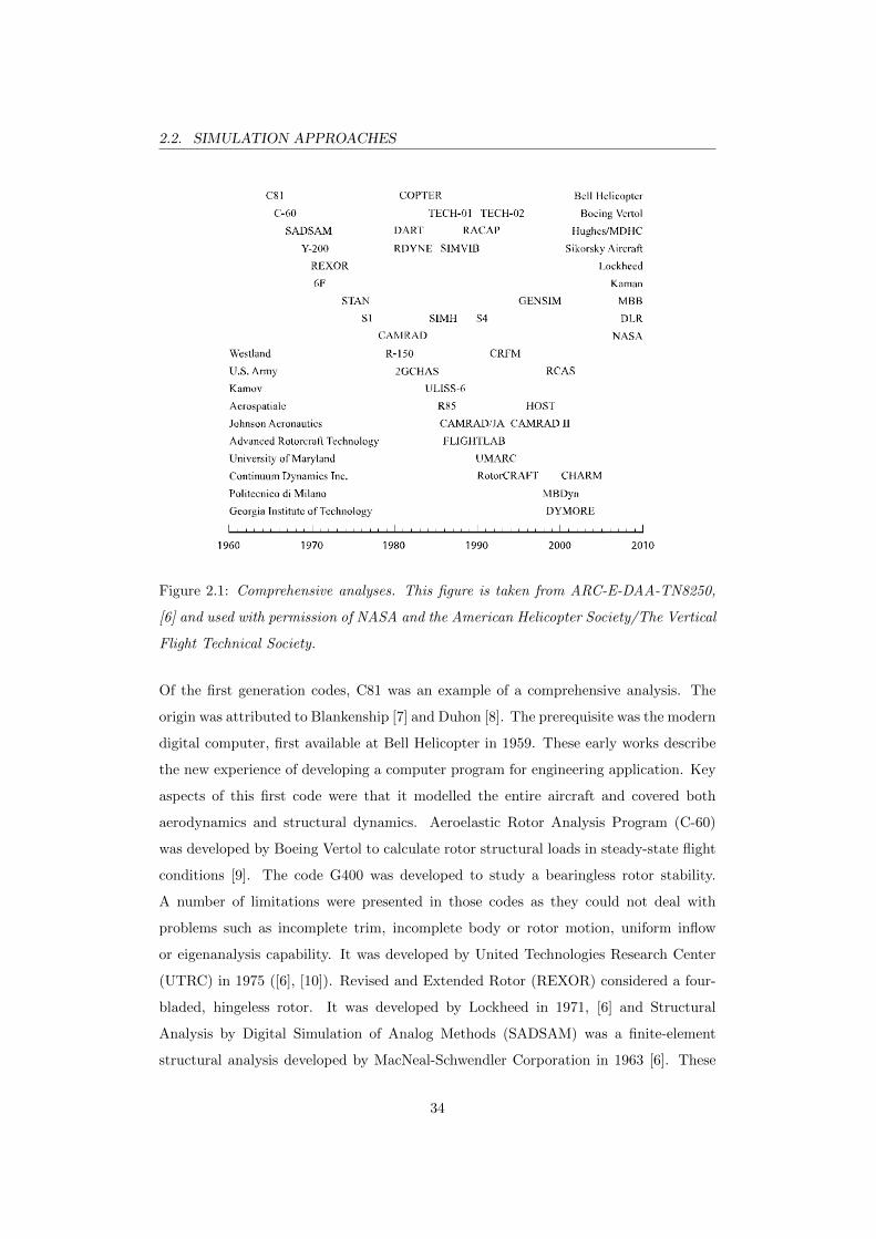
Figure 2.1: Comprehensive analyses. This figure is taken from ARC-E-DAA-TN8250,
[6] and used with permission of NASA and the American Helicopter Society/The Vertical
Flight Technical Society.
Of the first generation codes, C81 was an example of a comprehensive analysis. The
origin was attributed to Blankenship [7] and Duhon [8]. The prerequisite was the modern
digital computer, first available at Bell Helicopter in 1959. These early works describe
the new experience of developing a computer program for engineering application. Key
aspects of this first code were that it modelled the entire aircraft and covered both
aerodynamics and structural dynamics. Aeroelastic Rotor Analysis Program (C-60)
was developed by Boeing Vertol to calculate rotor structural loads in steady-state flight
conditions [9]. The code G400 was developed to study a bearingless rotor stability.
A number of limitations were presented in those codes as they could not deal with
problems such as incomplete trim, incomplete body or rotor motion, uniform inflow
or eigenanalysis capability. It was developed by United Technologies Research Center
(UTRC) in 1975 ([6], [10]). Revised and Extended Rotor (REXOR) considered a four-
bladed, hingeless rotor. It was developed by Lockheed in 1971, [6] and Structural
Analysis by Digital Simulation of Analog Methods (SADSAM) was a finite-element
structural analysis developed by MacNeal-Schwendler Corporation in 1963 [6]. These
34
2.2. SIMULATION APPROACHES
first generation codes were designed with very limited time and resources. In fact, they
were validated only for particular helicopter types or specific technical problems. Normal
Modes Aeroelastic Analysis (Y-200) was developed by Sikorsky Aircraft [11]. The flap-
lag-torsion equations of motion for the rotor blade were developed by Arcidiacono [12]
for an investigation of flutter, stall flutter, torsion divergence, and flap and flap-lag
stability. Stability Analysis (STAN) was developed by Messerschmitt-Bolkow-Blohm
(MBB) in the early 1970’s. This originated with the DF55 code, which was the first
complete helicopter simulation code at MBB. DF55 modelled the six aircraft degrees of
freedom and the blade flap motion, simulating the Bo105 hingeless rotor blade using an
equivalent offset hinge and a rigid blade [13].
On the other hand, a second generation of codes was characterized by an emphasis on
the study of the coupling of components. They were developed by the US Army and
the helicopter industry. The analysis was focused on the use of executive software for a
flexible and unified structure (see Figure 2.2).
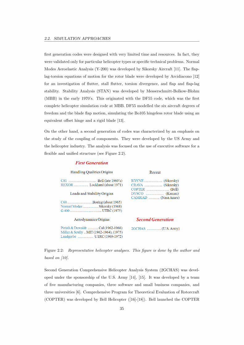
Figure 2.2: Representative helicopter analyses. This figure is done by the author and
based on [10].
Second Generation Comprehensive Helicopter Analysis System (2GCHAS) was devel-
oped under the sponsorship of the U.S. Army [14], [15]. It was developed by a team
of five manufacturing companies, three software and small business companies, and
three universities [6]. Comprehensive Program for Theoretical Evaluation of Rotorcraft
(COPTER) was developed by Bell Helicopter ([16]-[18]). Bell launched the COPTER
35
2.2. SIMULATION APPROACHES
program to produce the technology needed to support Bell products. The first opera-
tional version analyzed the aeroelastic stability of hingeless and bearingless rotors by
an eigenanalysis of linear equations. The equations were expanded in the uncoupled
vibration modes of the blade [6]. Rotor/Airframe Comprehensive Aeroelastic Program
(RCAP) was developed at McDonnell Douglas Helicopter Company [19], [20]. Rotor-
craft System Dynamics Analysis (RDYNE) was developed by Sikorsky Aircraft. The
blade elastic model was a new implementation of the equations of Arcidiacono [12].
Wake influence coefficients were obtained from the rotorcraft wake analysis [21]. 6F
was developed at Kaman Aerospace Corporation; it modelled a servo-flap control as
well as a conventional swashplate control [22], [23]. ULISS-6 was developed at Kamov,
and it modelled coaxial rotors including a vortex wake with prescribed geometry [24],
[25].
Additionally, the development of (1978-1980) comprehensive analytical model of rotor-
craft aerodynamics and dynamics (CAMRAD) gave birth to a number of theoretical
works such as the empirical dynamic stall model (1968-1969), vortex/blade interaction
(1969-1970), nonuniform inflow (1968-1970), rotor/wing dynamic stability (1972-1975)
and dynamic stability in free flight (1975-1976). From these works, the stability re-
search provided linearised equations of motion for the rotor [10]. S4 (4th generation
rotor Simulation program) was a high-resolution rotor simulation tool developed by the
German Aerospace Center (DLR) for investigations of rotor dynamics, vibration and
noise reduction, dynamic stall, blade airloads, and performance [26]. FLIGHTLAB was
developed as a real-time blade-element helicopter simulation by Advanced Rotorcraft
Technology, Inc. ([27]-[29]). This is a software development environment to support the
modelling of dynamic systems from a predefined library of physically based modelling
components. Computation of Rotor Aerodynamics in Forward Flight (RotorCRAFT)
was developed by Continuum Dynamics, Inc. [30]. The University of Maryland Ad-
vanced Rotorcraft Code (UMARC) was developed at the University of Maryland [31],
[32]. These codes were applied to a wide range of configurations including articulated,
hingeless, and bearingless rotors, servo-flap control, and tiltrotor aircraft. The Coupled
Rotor Fuselage Model (CRFM) was developed by Westland Helicopters in cooperation
with the Royal Aircraft Establishment [33], [34]. The objective was to predict the rotor
performance and loads and fuselage vibration in all flight conditions, both level and ma-
noeuvring flight, using a model of the coupled dynamics of the rotor and fuselage. This
required extending the model to multiple blades, taking into account coupling between
36
2.2. SIMULATION APPROACHES
the rotor and fuselage, and flying three-dimensional manoeuvres. GENSIM was Euro-
copter’s in-house helicopter simulation tool for global steady and unsteady performance,
flight mechanics, and loads calculations [35]. The blade aerodynamic model was based
on blade element/momentum theory with simple analytical downwash models and rigid
blades. Helicopter Overall Simulation Tool (HOST) was developed initially by Aerospa-
tiale [36]. It tackled the trim conditions problem. For trim, harmonic representation of
the motion was used with a Newton method to simulate the flight condition. DYMORE
was developed in the late 1990’s at the Georgia Institute of Technology [37], [38]. It was
a finite-element-based tool for analysis of nonlinear, flexible multibody systems, provid-
ing a general and flexible modelling approach that was modular and expandable. The
multibody dynamics approach was needed to deal with complex mechanisms of arbitrary
topology. Comprehensive Hierarchical Aeromechanics Rotorcraft Model (CHARM) was
developed by Continuum Dynamics, Inc. It was a comprehensive analysis applicable to
a wide range of rotorcraft problems including wake/surface interaction, vibratory air-
loading, and noise generation. The aerodynamic model covered multiple rotors, wakes,
and bodies, in free air and in an enclosure (including ground effect or a wind tunnel).
Rotorcraft Comprehensive Analysis (RCAS) system was developed for the U.S. Army
by Advanced Rotorcraft Technology, Inc. [39]. MultiBody Dynamics (MBDyn) was a
multibody, multidisciplinary code that provided a framework for integrated simulation
of complex multiphysics problems; it was developed at Politecnico di Milano [40], [41].
On the other hand, several of the existing mathematical modelling approaches to date
have been based on linearised models [42], [43]. Moreover, there exist some nonlinear
descriptions of helicopter dynamics but only for reduced order models [44] or without
taking into consideration the interaction of the main rotor with the fuselage [45]. [46]
discussed a multibody system simulation architecture capable of generating the dynam-
ical equations of a multibody system symbolically, automatically create the computer
code to simulate the equations numerically, run the simulation and graphically display
the results. In this work, the equations were described in a theoretical manner but
analytical form of them was not provided. The Modelica-Dymola environment has been
also used previously to address the problem of modelling helicopter dynamics ([47]-[49]),
where parametric and reconfigurable helicopter dynamic models were presented but the
dynamical equations of the main rotor were not presented. Some other authors (see [50]
as an example) have used MAPLE to formulate the complete set of nonlinear equations
of motion for a coupled rotor and fuselage system. This symbolic software automati-
37
2.2. SIMULATION APPROACHES
cally converted the equations of motion into C, Fortran or Matlab. The compiled source
code can be accessed and numerically integrated by the dynamic simulation software
Simulink. It was then used to generate the time history of the blade’s and fuselage’s
motion. In order to obtain the nonlinear equations of motion, a combination of several
codes was needed, which complicated the process in great manner and increased the
execution time.
There exist several other mathematical modelling approaches to study helicopter dy-
namics; they comprise nonlinear equations of motion derived by Lagrangian methods,
but they lack of an automated modelling tool in order to expand the equations and in-
corporate a control system/simulation environment such as Matlab, Maple or Simulink,
see ([51]-[53]) as examples. Some other approaches used within the context of helicopter
dynamics do not address directly the modelling aspects of it, but focus on stability anal-
ysis instead. In these cases, some sort of modelling methodology is needed, being based
in most cases on linearised models, reduced order models [54] and more rarely on non-
linear models for which the integration process was tedious, computationally expensive
and state space representation of the system or dynamical equations of motion are not
presented to the user [38], [55], [56]. In addition to this, an early work using ADAMS
was done by Bertogalli [57], this work shows the results of a study aiming at the de-
sign of an ADAMS based simulation program for the dynamics and aerodynamics of
the main rotor of the Agusta A109c helicopter. The complexity of the system under
investigation (rotor blade flexibility, unsteady aerodynamic loading, non-uniform and
time-varying wake) required use of ADAMS’s features as user-written subroutines and
linear systems simulation and the development of subroutine (CONSUB) for simula-
tion management and control [57]. On the other hand, Bianchi dealt with ADAMS
and the helicopter tail rotor analysis, they presented some major results obtained from
the dynamic simulation of a partially flexible tail rotor model of an Agusta helicopter,
being the aim to investigate the features of ADAMS as a mechanical system simula-
tion tool through an application to a case of interest for Agusta. The results obtained
from the simulations performed were satisfactory, but the authors admitted that much
work was still needed to be carried out in some areas [58]. Brown developed a com-
putational tool, Vortex Transport Model (VTM) that allows to analyse aerodynamic
and dynamic performance on several rotor helicopter configurations under both steady
and manoeuvring flight conditions. The aerodynamical module uses a computational
solution of the Navier-Stokes equations. It is expressed in vorticity velocity form in
38
2.3. MAIN ROTOR
order to simulate the evolution of the wake of a helicopter rotor ([59]-[62]). Some of the
more challenging aspects of modelling the mechanical dynamics of rotorcraft systems
are addressed in this work and the corresponding dynamics are analysed. The modelling
tool is VehicleSim, [63], a multibody systems software package that derives a realistic
nonlinear model of the fundamental dynamics of an articulated rigid-bladed rotorcraft.
One of the advantages of using VehicleSim is that compared to hand derived equations
(usually prone to errors), the automated equations give an accurate representation of
the complex system’s dynamics. Also, due to its software engineering features, it uses
a reduced execution time. VehicleSim uses an advanced form of Kane’s equations and
applies extensive algebraic and programming optimization methods to achieve high effi-
ciency. Within the context of automatic modelling of system’s dynamics, [64] provides a
method for representing rigid multibody systems in symbolic form by means of AutoSim
(previous version of VehicleSim).
2.3 Main Rotor
The main system of a helicopter is the rotor as it allows the helicopter to fly. The main
rotor has two different parts: the rotor and the blades linked to it. The rotor has an
influence on the blade’s displacement. It is known that blades have three degrees of
freedom: flap, lag and feather influenced by the main rotor.
Flap, lag and feather are studied as independent degrees of freedom. In fact, Majhi and
Ganguli [65] derived the general equation describing the blade’s flap dynamics for a large
flap angle and large induced inflow angle of attack. Numerical simulations were carried
out solving the nonlinear flap ordinary differential equations for steady state conditions
and the validity of the small angle approximations was examined. A semi-empirical
dynamic stall aerodynamics model was used. The results showed that a small flap angle
assumption, and to a lesser extent, the small induced angle of attack assumption could
lead to inaccurate predictions of blade flap response under certain flight conditions for
some rotors when nonlinear aerodynamics were considered [65]. The coupling between
blade flap and lag motions was tackled in the work by Pavel [66]. They studied the
Micon 1500/600 lead-lag instability on high wind speed runs when the blades were
operating in the stall region. This work derives the coupled flap-lag equations of motion
for rigid blades and axial wind at the rotor hub with hinge offsets and spring restraints.
39
2.4. TAIL ROTOR
The equation of motion was extended and blade flexibility was introduced in the model.
In addition to this, the variation of the coupled flap and lag eigenvalues with the feather
angle were presented in the complex plane for various wind speeds. The study concluded
that coupling between blade flap and lag motions would occur when the wind turbine
was operating in the stall area [66].
Ormiston and Bousman [67] used the AH-56A Cheyenne helicopter to determine fun-
damental stability characteristics of the hingeless rotor when considering the flap and
lead-lag degrees of freedom of a single blade. This work was carried out in the absence of
available experimental data, a model rotor was designed and tested to validate the the-
oretical analysis instead. As a result of these investigations, various applied approaches
were suggested for hingeless rotor blades inherent stability improvement.
Eigenvalues and eigenvectors analysis have an extensive use in rotorcraft data analysis.
Al-jawi and Mohamad [68] studied the stability of a rotorcraft with five degrees of body
freedom. The study focused on linear formulations of the system. Eigenvalues were
used to obtain the system’s stability boundaries, while the eigenvectors determined the
blade’s behaviour. This work proved that in the case of identical blades, the blade’s
complex eigenvectors are orthogonal to each other.
Although many previous analyses were carried out, Du Val presented an extensive study
dealing with the inertial dynamics of a fully articulated stiff rotor blade. The model
used in this derivation included a hinge offset and a six degrees of freedom rotor shaft.
The main objective was to facilitate an organized program for simulation applications.
The results were compared to the flap and lead-lag equations used in the Rotor Systems
Research Aircraft (RSRA) simulation model [69]. In order to understand the rotorcraft
flight dynamics, the work presented by Hohenemser [70] was reviewed in here, the author
dealt with the basic rotor design parameters that affect the flight dynamics, analytical
modelling techniques as well as mathematical analysis techniques (nonlinear modelling).
2.4 Tail Rotor
The tail rotor plays a fundamental role in a Sikorsky configuration helicopter. In order
to model and simulate the tail rotor in VehicleSim, several contributions were reviewed.
A complete report on the tail and its design was presented by Wiesner and Kohler [71].
40

2.5. FUSELAGE
This work is a general guideline for a preliminary design of tail rotors operating at
low speed and hover flight. The directional control problems of single rotor helicopters
under certain conditions such as altitude, wind speed and direction amongst others,
were studied. The database used to carry out this work was wind tunnel tests of a tail
rotor helicopter model. The tests were run in and out of ground effect, in various wind
speeds up to 35 knots and with varying wind azimuths. In addition to this, parameters
that affect flying qualities and structural loads were studied together with feather-flap
coupling, tail rotor shaft sweep, pedal control rate limiting, etc.
An early work on helicopter directional stability and control at low speed flight was
presented by Amer and Gessow. In here, the tail rotor collective feather was studied
using charts, these were based on equations for the collective feather of a tail rotor at
low forward speeds in terms of its forward speed, tip speed, thrust coefficient, solidity
and yawing speed of the helicopter. As a consequence of this, tail rotor design studies
of directional trim and control response at low forward speed could be carried out. The
charts were used to study the main rotor stability derivatives of thrust with respect to
the collective feather and angle of attack at low forward speeds [72].
Pereira et al. analysed the influence of the positive pitch-flap coupling on the flap
response of an articulated tail rotor blade. The geometric parameters were similar
to those of the AS355 Twin-Engine Squirrel helicopter. Mathematical models were
presented for hovering flight and forward flight conditions. These allowed to model the
tail rotor implemented in this thesis [73].
Stanislawski presented a simulation method for calculating tail rotor loads and blades’
deflections in a directional manoeuvre. Additionally, aerodynamic forces acting on a
blade segment at a given azimuth position on the tail rotor disc were obtained using
blade element theory. Simulations calculations concerning the work of tail rotor at
direction manoeuvre of helicopter in hover and level flight condition were performed
[74].
2.5 Fuselage
The fuselage is an essential part of the helicopter and it plays an important object of
study in this thesis. The fuselage has been studied and analyzed as a fundamental part
41
2.6. EQUATIONS
of the helicopter as shown in Guo-cai’s work. In here, the authors derived nonlinear
differential equations and integrated them in the time domain to yield responses of rotor
blade flap, lead-lag and fuselage motions. The objective of this work was to accurately
predict the dynamic instabilities of a helicopter coupled rotor-fuselage system. Fast
Fourier Transform (FFT) was used to estimate the modal frequencies, and Fourier se-
ries based moving-block analysis was employed in the predictions of the modal damping
in terms of the response time history. Time-domain methods and eigenanalyses were
applied to predict dynamic instabilities and compared to wind tunnel test data of refer-
ence. The results showed excellent agreement between analytical and experimental data
in the ground resonance cases. Thus, it could be applied to the dynamic stability analy-
sis of rotor-fuselage coupled systems together with nonlinear and unsteady aerodynamic
models as well as nonlinear blade lag dampers [75].
Coupling mechanics have an important role to play in helicopter’s behaviour. Keller
examined the off-axis response problem using an analytical model, with the goal of
understanding the coupling mechanics. The effects of a wake distortion created by the
pitch rate were included by an induced velocity model. The inclusion of these effects
results in a significant change in the lateral flap response to a steady pitch rate. The
results showed that the inclusion of an induced velocity variation due to the shaft rate
improved the correlation in the pitch response to lateral cyclic inputs. The proposed
inflow model was coupled to the full rotor-body dynamics model and comparisons were
carried out between the existing model and flight test data for a UH-60 in hover [76].
Simulation models as well as their development and validation processes play a main role;
Manimala et al. described the development and validation of a high fidelity simulation
model of the Bell-412 in the FLIGHTLAB environment for handling qualities and flight
control investigations. The following main steps were carried out, rotor hub design,
modelling of the hub and blade retention, blade aerodynamics description, rotor inflow,
tail rotor and fuselage modelling, and finally model validation [77].
2.6 Equations
An extensive body of literature exits on the equations that govern helicopter’s rotors.
Early work was published by Zbrozek, the mathematical expression for describing the
42
2.6. EQUATIONS
moment due to blade’s angular acceleration in flap motion and the moment due to
centrifugal force were presented. The blade’s angular velocity and acceleration were
expressed as functions of the angles of tilt when the tip-path plane was tilted with
respect to the shaft in the plane of oscillation and in the plane perpendicular to it.
Also, the blade inertia was treated through the values of blade inertia number, and its
influence over the acceleration when the blades were heavy. The mathematical analysis
of the dynamic blade flap during a simple harmonic motion of the helicopter provided
the existence of angular velocity and acceleration derivatives. The effect of the angular
acceleration derivative on the helicopter’s dynamic stability was small, as a result, the
usual values of blade inertia number were neglected. The effect of the frequency ratio
ν = ν/Ω (ν is the frequency of shaft oscillation and Ω is the rotor’s rotational velocity)
on the values of the rotor’s derivatives was also small, due to the fact that for all
helicopter models built to dynamic and aerodynamic scale, the value of ν was likely to
be much less than 0.1. It was for the case of helicopters with heavy blades i.e., γ < 8
(where γ is the blade inertia number), that the effects of the acceleration term and the
frequency ratio need to be taken into account [78].
Stewart performed a large study of blade’s flap motion. It treated the flap angle as
harmonics and derived a mathematical expression for flap and pitch. At high tip speed
ratio and blade’s collective pitch large values, where blade stalling can occur on the outer
sections of the blade, the amplitude of some of the flap harmonics may be increased
considerably [79].
The work by Lowis obtained the transient solution of the helicopter’s rotor blade flap
motion as well as the effective damping of the motion determined for high tip speed
ratios. The equation for flap motion was presented for an untwisted blade with constant
chord and did not bend or twist. The flap hinge was assumed to be on the axis of rotation
and perpendicular to the spanwise axis of the blade i.e., δ3 = 0. Furthermore, regions
of reverse flow over the retreating blade were not taken into account. The solution of
the flap equation of motion led directly to the parameter which measures the stability
of the motion using the method proposed by the author [80].
Wilde et al. solved the blade flap equation taking into account the reversed flow region
but neglecting stall. The effects of springs, dampers, offset and δ3 hinges were also
considered. The flap behaviour of articulated rotors was studied for high tip speed ratio
values. It was shown that flap motion became unstable about µ = 2.25 (µ is tip speed
43
2.6. EQUATIONS
ratio), and it slightly depended on the Lock’s inertia number. The flap amplitude in
response to a change of disc incidence was larger as µ increases. Furthermore, an offset
hinge had little effect on the blade flap amplitude. The effect of a δ3 hinge on a fully
articulated blade was approximately the half of the flap, over the whole range of µ,
when δ3 angle was 30 degrees. Finally, viscous dampers were effective in restraining
blade flap and it appeared that little was gained by using springs [81].
The unsteadiness of aerodynamic, inertial and gravitational forces generates vibratory
loads and stresses which act on the rotor [82]. In this work, blade forces were studied
together with aerodynamic, inertial and gravity forces. The aerodynamic loads were
generated by the unsteady nonuniform wind environment. Inertial blade loads included
centrifugal tension due to rotation as well as lead-lag and flap loads due to Coriolis
forces arising from blade oscillations, and gyroscopic forces due to precession of the
rotor shaft to maintain alignment with the wind velocity vector.
When the flap and lag are studied independently from each other, the Coriolis force can
be neglected and the centrifugal force must be considered on each case. Stafford and
Giurgiutiu studied these uncoupled equations for the case of the Timoshenko beams.
Solutions were obtained using the Frobenius power series method. The principal advan-
tage of this approach was the exact representation of the centrifugal force [83].
Later on, this work was extended and coupled flap/lag, together with pitch degrees of
freedom were included in the equations [84].
Vyas derived the equations of motion of a blade mounted on a disc rotating with vari-
able angular velocity. The acceleration of the disc was constant. In addition to this,
the calculus of variations method was used to obtain the equation that governs the
subsequent free vibrations [85].
Chen did a complete work on the flap-lag nonlinear dynamical equations of motion.
Three hinges sequences were used in order to obtain the equations: lag-feather-flap, flap-
feather-lag, flap-lag-feather. The Lagrange method was used to work out the coupled
flap-lag equations of motions [86].
44
2.7. STABILITY
2.7 Stability
The stability is a fundamental aspect that should be taken into account when modelling
any type of vehicle. Several contributions were reviewed in this sense. An early work
was done by Gessow and Amer where static stability with angle of attack, speeds and
damping due to a pitching or rolling velocity were studied. In hovering flight conditions,
the helicopter has neutral static stability with respect to attitude changes. On the
other hand, the helicopter showed positive static stability with respect to changes in
translational velocity. The resulting motion of the helicopter oscillated if disturbed from
hovering conditions. The period of oscillation depended on two factors, the moments
appearing due to changes in speed and the moments due to the helicopter’s angular
velocity. In forward flight, static stability with attitude changes and static stability
depending on speed changes were considered as well. This work concluded that the
helicopter’s rotor is statically stable with speed and statically unstable with angle of
attack. The static stability is unaffected by centre of gravity shifts if the moments
are not contributed by components other than the rotor. If there exit other moments
contributions such as a fixed tail surface, the static stability is as well affected [87].
Reeder and Gustafson [88] studied the impact of the angle of attack in forward flight
on stability as well as the control sensitivity in hovering and the control forces following
control actions for manoeuvring. Rotor instability appeared as a result of flap and
increased in severity with increasing speed.
Root locus techniques were used to study the stability and the various modes of motion.
Curtiss considered some aspects of the prediction of flap and lag instabilities on hingeless
rotor blades whilst hover flight. The dependence of the characteristic modes on blade’s
pitch angle was examined for various analytical models using root locus techniques.
Prediction of flap-lag stability using a single bending mode for each degree of freedom
was examined. As a result of this study, prediction of flap-lag stability was very sensitive
to the model used in modelling the rotor blades aerodynamic and elastic characteristics.
Furthermore, the equivalent lumped spring constants for either the parallel or series
spring model can be determined from the results of an elastic analysis of a rotor blade
[89].
45
2.8. VIBRATIONS
Ormiston and Hodges examined the linear stability characteristics of rotor blade flap-lag
oscillations in hover flight. The study focused on the effects of pre-cone, variable elastic
coupling, pitch-lag coupling and, the aerodynamics of the induced inflow. The effects
of kinematic pitch-lag coupling on flap-lag stability are highly dependent on the elastic
coupling for stiff in-plane rotor blades, but not for soft in-plane ones. This work showed
that the flap phase response for pitch excitations was significantly altered by elastic
coupling. This implied that coupled rotor-fuselage dynamic equations should include
the rotor blade’s in plane degree of freedom [90].
Antequera et al. designed a UAV controller based in the eigenvalues assignment tech-
nique. The system (which was initially unstable) was satisfactory stabilized. In addition
to this, the flexibility of the eigenstructure assignment improved the system’s response
by applying a recurrent algorithm for selecting new eigenvalues and/or eigenvectors for
decoupling purposes [91].
2.8 Vibrations
Vibrations constitute the major source of unwanted oscillations in helicopter systems
and one of the main areas of active research. During years, efforts have been devoted to
the detection, characterization, analysis and suppressions of unwanted vibrations. The
existing literature covers most of the aspects already mentioned.
In this section, some of the most relevant contributions in this field are revised. Bazov
states the existence of many sources of exciting forces which cause forced vibrations in
helicopter. Such sources include the main and tail rotors, power system, transmission
gearboxes and shafts. Each of these sources creates exciting forces with a definite
frequency. The lowest exciting force frequency is that of the main rotor. It may be
found from the formula nmr = nsk where nmr is the main rotor exciting frequency; ns
is the main rotor rps and k is the number of main rotor blades. The frequency of the
main rotor exciting forces varies in the range of 8− 16 Hz. The tail rotor excites forces
with a frequency of 10− 60 Hz. The transmission shafts and gearboxes create a higher
frequency of the exciting forces: from 50 to several hundred vibrations per second. The
power plant yields a broad spectrum of exciting forces with frequencies of 600 − 1000
Hz. The primary forced vibration source is the main rotor with hinged blade support.
46

2.8. VIBRATIONS
Blade oscillations relative to the hinges are also the source of several vibrations [92].
Chen et al. analyzed blade’s nonlinear vibrations with varying rotating speed. Thin-
walled beams were considered in this study because they have been used in a broad range
of fields including aerospace and mechanical industry. The model of rotating thin-walled
beams could be employed in the designs of turbine blades, helicopter blades, etc. On the
other hand, the vibration analysis plays a central role in reliability of rotating blades.
Therefore, a comprehensive understanding of their vibration characteristics, especially
nonlinear behaviour is of importance to predict their dynamic response to external
excitations. As a consequence, they proposed an analytical expression for the varying
angular velocity case [93].
The work made in Santos et al. presented a theoretical and experimental contribution
to the problem of rotor and blades dynamic interaction. A simple test rig, built by a
mass and spring system attached to four flexible rotating blades was used to validate the
mathematical models. Only lateral displacement of the rotor in the horizontal direction
was taken into account. Gyroscopic effects due to angular vibrations of the rotor were
eliminated in the test rig by attaching the rigid rotor to a flexible foundation. The
blades were modelled as Euler and Bernoulli beams. Indeed, the linear model could
correctly estimate parametric vibrations in a short range of low rotational speed, where
the stiffening effect was of minor importance. Superharmonic vibration associated to the
movement of the flexible rotating parts, with large amplitude, could only be detected
with the help of the fully nonlinear model [94].
Keysan showed that the harmonics from a rotor slotting machine can be utilized for con-
trol or diagnostic purposes. In the existing literature, rotor slot harmonics are mostly
utilized for condition monitoring. The study illustrates a new approach to the identifi-
cation of rotor slot harmonics which consumed very little computation time [95].
Tuma studied the rotor vibration’s stability. The rotor was considered to be under the
influence of a perturbation caused by external forces. The perturbation force was as-
sumed to be rotating at the angular velocity ω, which was considered to be independent
from the rotor angular velocity Ω. The rotor was perturbed by the non-synchronous
force with respect to the rotor angular frequency. The equation of motion contained
complex variables as a function of time. The work showed how to solve such equation
using Simulink [96].
47

2.9. AERODYNAMIC ENVIRONMENT
Schulz studied possible isolation methods for a helicopter. The compensation of vibra-
tions generated by the rotor of a helicopter and transmitted to the cabin is of great
importance for rotorcraft design. These vibrations occur at discrete frequencies i.e.,
rotor blade harmonic frequencies. For the compensation of vibrations, a control law
was derived, which isolated the cabin from the rotor/gear-box unit at the disturbance
frequency, by use of electro-hydraulic actuators [97].
In the area of vibrations control of helicopters there are several contributions that up to
now investigate different methods ranging from IBC (Individual Blade Control) to HBC
(Harmonic Blade Control) among many others. The problem of vibration’s control is
not within the scope of this thesis.
2.9 Aerodynamic Environment
The aerodynamic forces around the helicopter system are the ultimate reason for its
flight. Therefore, studying the nature of these forces, obtaining a good mathemati-
cal representation and good understanding of them becomes a necessary task before
approaching further issues on helicopter research.
Helicopter aerodynamics have been studied since the first concept of these vehicles was
conceived and therefore it counts with an endless amount of existing relevant literature.
Aerodynamic force modelling has a great impact in the helicopter simulation research
field. The following review is done in order to understand the main aspects of the
helicopter flight by using blade element theory as well as the parameters that this
method involves.
Blade element theory is commonly used in helicopter flight simulation models. The
theory consists on dividing a blade into various blade elements orientated in the chord
wise direction; each element is aerodynamically independent from the neighbouring
elements. This allows the use of 2D aerofoil characteristics in order to determine the
forces and moments produced on the blade [98].
An early work in the literature that used blade element analysis was carried out by
Castles Jr. and New. A set of blade element equations were derived by giving the
relation between the thrust and flight path velocity components and the equilibrium
48
2.9. AERODYNAMIC ENVIRONMENT
blade angles, torque and in-plane forces. The inflow angle and blade angle of the blade
elements were taken into account for small angles [99].
Myers provided basic data on helicopter rotor blade motion; photographic records of the
behaviour of a blade in flight were obtained with a conventional single rotor helicopter.
In addition to this, some fundamental mathematical expression and values such as inflow
ratio, solidity, tip-loss factor amongst others, were also provided [100].
Majhi and Ganguli examined the small flap angle approximations for steady state flight
conditions and solved the nonlinear flap ordinary differential equation using numeri-
cal simulations. This work, showed how the blade element analysis allows to develop
an aerodynamic model that deals with rotor blade flap motion considering nonlinear
aerodynamics [101].
Vilchis et al. studied the aerodynamic forces and provided its algebraic expressions
as well as the torques used to deduce the generalized external forces acting on the
helicopter, this work presented the development of a nonlinear control strategy for a
VARIO scale model helicopter [102].
In Dingeldein and Schaefer, some fundamental aerodynamic aspects were studied in
order to analyze the aerodynamic characteristics of a single rotor helicopter in forward
flight [103].
Mikhailov et al. analyzed blade motion stability in forward flight, as for a helicopter, the
unstable coupled flap, torsional and lag oscillation that occurs due to the interaction of
inertial, aerodynamic and elastic forces of main rotor blades may be detrimental towards
stability. The equations of a coupled blade motion were obtained using blade element
theory [104].
Salazar developed a helicopter mathematical model with main and tail rotors, the model
consisted of six nonlinear equations. Some simulations were carried out under specific
flight conditions and each induced velocities were also used according to these. Pertur-
bations such as wind crossing or vibration engine were considered in order to build up a
robust model. Simulations of lateral and ascend flight could be found using the mathe-
matical model. This approach was suitable to simulate and to control a helicopter, as
a result the model could be used to control autonomous radio helicopter or automatic
helicopter pilot as well as to build a flying computer training program [105].
49
2.9. AERODYNAMIC ENVIRONMENT
Siva et al. studied the effect of uncertainties on performance predictions of a helicopter.
They considered uncertain variables, the main rotor angular velocity, main rotor radius,
air density, blade chord and blade profile drag coefficient. The propagation of these
uncertainties in the performance parameters such as thrust coefficient, induced velocity
amongst others, were studied. In the formulation of this work different flight regimes
were dealt as well as the aerodynamic environment involved in these regimes [106].
Rotor wake modelling was extensively covered by [59]. The author developed a compu-
tational helicopter rotor wake model, based on the numerical solution of the unsteady
fluid dynamic equations that governs the generation and the convection of vorticity in
the helicopter rotor environment. The model predicted the wake structure for cases such
as hover and forward flight. On the other hand, Griffiths and Leishman [107] developed
a free-vortex wake model in order to examine the rotor’s problems on rotor interference
as well as rotors operating in ground effect. Rotor performance for dual rotor systems
under various combinations of gap and stagger was studied and the predicted results
were compared to experimental measurements. For a dual rotor system the free-vortex
model results provided a beneficial aerodynamic interference effect in hover flight for a
limited range of stagger spacings. Furthermore, a new momentum theory for the perfor-
mance of overlapping dual rotors with gap was obtained. This was used as a reference
solution and compared to the free-vortex results and experimental data for larger over-
lap ratios. The free-vortex results confirmed that ground effect on rotor power depends
on both the rotor height off the ground as well as flight speed. Results for hover and
forward flight were found to be good agreement with limited experimental measure-
ments. The authors indicated that additional validation of the approach was essential
to improve the confidence in the method.
Leishman et al. [108] reviewed the theoretical basis and numerical implementation of one
class of free-vortex filament methods, which proved to be robust and flexible numerical
methods that should be taken into account to the prediction and analysis of helicopter
rotor wakes. Various examples of the application of free-vortex filament methods to
helicopter rotor problems were provided, including the wake structure and performance
of single and multirotor configurations, the flight in ground effect, the effects on the
wake dynamics during manoeuvring flight conditions, and the descending flight through
the vortex ring state. The author indicated that free-vortex filament models considered
for helicopter rotor wake analyses got predictive capability, further algorithmic improve-
50
2.9. AERODYNAMIC ENVIRONMENT
ments and better validation of the methods were required. In particular, research was
required to integrate rigorously the blade wake and tip vortex models and viscous ef-
fects, for example turbulent diffusion of vorticity, into vortex filament methods. In [109]
the helicopter rotor wake is also studied. In here, Bhagwat and Leishman studied the
helicopter rotor wake stability in hover and axial flight by using eigenvalue analysis. The
rotor wake was shown to be unstable, with the tip vortices exhibiting various possible
unstable deformation modes.
Analytical helicopter rotor aerodynamics were studied by [110]. The authors presented
a method for predicting the onset of the vortex ring state in terms of a model for the
propagation and growth of disturbances within the rotor flow. Numerical simulations of
the onset of the vortex ring state provided that the transition into the vortex ring state
was increasingly gradual as the acceleration of the rotor was increased. The combination
of high forward speed and vertical acceleration, the vortex ring state could be replaced
by a qualitatively different, highly transient state where the collapse of the wake into
the toroidal form that was usually associated with the onset of this flow condition was
suppressed. The absence of an abrupt and universal transition marking the onset of
the vortex ring state under accelerated flight conditions complicated the application of
simple analytical models. This generated that the specific details of the time-dependent
dynamics of the rotor wake as well as its interaction with the rotor could not be ignored.
Aerodynamic simulation was as well tackled by Phillips and Brown for brownout prob-
lem analysis [60]. In this work, Brown’s Vorticity Transport Model (VTM) was used to
simulate the development of the dust cloud that could form around a helicopter when
operated in dusty or desert conditions. In addition to this, the flow field around a tan-
dem rotor configuration was simulated for the final stages of landing. VTM simulations
provided that for a tandem rotor helicopter the sudden growth of the dust cloud that
was responsible for the onset of brownout was due to a change in mode within the flow
field surrounding the aircraft. At higher advance ratios the flow was dominated by a
strong ground vortex that was created by the tail rotor.
Computational Fluids Dynamic (CFD), is an extensive method of research. An early
work in this field applied to helicopter research was carried out by Caradonna. In this
work, the author indicated that the performance of rotary wing aircraft was limited
by a host of aerodynamic problems. The ability to design rotorcrafts with confidence
required a new order of aerodynamic predictive technology that was both true to the
51
2.10. UNMANNED AERIAL VEHICLES (UAVS)
basic flow physics and readily usable by industry. CFD approaches can solve issues
such as rotor wake prediction, compressible aerodynamics, interaction problems, etc
[111]. In [112], the rotor interactions with vortices were studied as these are common
problems, especially in descent or manoeuvre and the Blade/Vortex Interaction (BVI)
is the predominant noise source. The ability to predict the wake was the basic problem
in BVI aeroacoustics and the problem was considered from a CFD point of view. It
was suggested that new approaches to CFD should be taken into account as methods
in which vortex cores were not resolved.
2.10 Unmanned Aerial Vehicles (UAVs)
UAVs have been in the past years object of several studies from many different points
of view. Industry and government institutions all over the world have invested great
amount of money in investigation and developing these types of systems. Research con-
ducted in the field of UAV ranges from dynamical modelling, mechanical and technical
improvements, control of trajectories, control of groups of these vehicles, communication
systems, etc. UAV modelling has been also explored in this work.
UAV modelling and simulation was analyzed by Velez et al. They presented a Rapid
Software Prototyping Environment (RSPE) for the design, simulation, and real time
implementation of a control system for an autonomous mini-helicopter. The software
prototyping environment consisted of diverse modules such as mini-helicopter simulation
model, controllers, ground control station, a navigation filter and linearization and
parameter identification tools [113].
Johnson and DeBitett developed a simulation capability to support the design, develop-
ment, and test of the navigation, control, guidance, and vision processing subsystems,
as well as human machine interfaces and procedures for Unmanned Vehicle Systems
[114].
Vilchis et al. presented the development a nonlinear model and a nonlinear control
strategy for a VARIO scale model helicopter. The contribution focused on the partic-
ular case of a reduced order model i.e., three degrees of freedom where a scale model
helicopter mounted on an experimental platform was represented. The theoretical de-
velopment was illustrated using numerical results and experiments. Additionally to this,
52
2.10. UNMANNED AERIAL VEHICLES (UAVS)
the robustness with respect to parameter uncertainties was also studied [102].
Main rotor loads and tail rotor force fluctuations are in the majority of cases the primary
source of unwanted vibrations in these type of vehicles.
The work done by Cai et al. presented a comprehensive design methodology for con-
structing small-scale UAV helicopters. The systematic design procedure, which included
hardware component selection, design and integration, as well as experimental evalu-
ation, was utilized to construct a fully functional UAV helicopter. In this work, the
author studied the vibration sources in UAV helicopters and three sources were identi-
fied: rotation of the main rotor (30.8 Hz), rotation of tail rotor (143.4 Hz) and engine
as vibration source (260.5 Hz). These frequencies are estimated based on a governed
motor speed at 1850 rpm (revolution per minute) [115].
Dunbabin et al. carried out the design and construction of an integrated isolated vision
and sensor platform and landing gear for the CSIRO autonomous X-Cell helicopter.
In this work, the authors studied various vibration sources. These can be mechanical,
aerodynamic and from normal flight motion with a broad amplitude and frequency
spectrum. A range of vibrations for autonomous helicopter was given as: main rotor
speed 25 Hz, tail rotor speed 113 Hz and engine speed 160 Hz [116].
A fundamental aspect in UAV helicopter modelling is the gyroscopic system that is used
to stabilize the system under the action of different flight conditions. Affanni described
the design, development and dynamic characterization of a high performance MEMS-
based gyroscopic control system for the yaw channel of Unmanned Aerial Vehicles for
aerobatic manoeuvres. The yaw channel was composed by a servomotor and the tail
blades. A transfer function between the normalized servomotor position and the yaw
angular rate was provided. A new asymmetrical controller was implemented to com-
pensate the torque of the main rotor. The yaw rate characterization demonstrated a
high and constant pirouette speed. Indeed, aerobatic tests demonstrated high accuracy
entry into the manoeuvres [117].
Kim and Tilbury presented a mathematical model for a UAV helicopter robot, focusing
on the dynamics of the flybar. The work demonstrated how the flybar’s flap increases
the helicopter’s stability robot as well as assists on its actuation. In addition to this, the
equations of motion for a six degrees of freedom model with a flybar degree of freedom
were derived, system identification experiments and results were presented to verify the
53
2.11. CHAPTER SUMMARY
mathematical model structure and to identify model parameters [118].
Cunha and Silvestre studied Bell-Hiller stabilizing bar dynamics. They presented a
helicopter dynamic model, it was parameterized as a Vario X-Treme acrobatic helicopter.
The simulation model included a rigid body, main rotor flap and the stabilizing bar
dynamics. Solutions for a set of trimming trajectories were identified and discussed.
The Bell-Hiller stabilizing bar is a mechanical blade pitch control system that generates
helicopter stability. It is a standard component of model-scale helicopters. Stabilizing
bars provide roll and pitch rates’ dynamic feedback. In fact, the system consists of a
flybar, a teetering rotor placed at a 90 degrees rotation interval from the main rotor
blades and tipped on both ends by aerodynamic paddles. The stabilizing bars and its
impact on the overall helicopter dynamics were analyzed [119].
Lau et al. presented a new method based on the fact that when the angular momen-
tum of the spinning rotor was disturbed by the incremental lift along the main blades
due to the varying cyclic pitch angle controlled by the servo mechanisms, the off-axis
moments were induced to counteract the changes of the angular momentum according
to the gyroscope principle. This work did not explain the responses by which the hin-
geless helicopters behave, it just quantifies a set of coupled auxiliary responses. The
authors simulated the derived analytical forms and validated in experiments using the
instrumented hingeless helicopter. It is concluded that using the proposed treatment,
the unintuitive off-axis responses can be predicted and the on-axis responses can also
be quantified [120].
These are, of course just a short number of contributions existing in the field of UAV
literature. At the present, the existing amount of articles and works in this field is vast
and will continue to increase in the near future. The references here mentioned are just
a short selection of them in order to illustrate the main lines of research being carried
out in the area of UAV research.
2.11 Chapter Summary
In this chapter existing relevant literature in various helicopter’s topics has been revised.
The first part was devoted to review the state of the art of several existing simulation
approaches. In this work, it will be shown how symbolic software is advantageous with
54
2.11. CHAPTER SUMMARY
respect to previous numerical software approaches such as ADAMS.
On the other hand, topics such as main and tail rotors, fuselage, dynamic equations, sta-
bility, vibrations, UAVs and aerodynamic environment modelling were also reviewed. In
particular, for the aerodynamic literature review, blade element theory was thoroughly
revised as this is the theoretical approach taken in this work for the aerodynamic mod-
elling still, other aerodynamic approaches were revised such as CFD and VTM.
In conclusion, the chapter reviewed the state of the art in helicopter field modelling
aspects and the existing simulation approaches revision showed that VehicleSim can
provide multiple benefits when used as a simulation tool.
In fact, this is the first (to the author’s knowledge) work existing in rotorcraft dynamics
and aerodynamics made using VehicleSim as the only modelling tool.
55
Chapter 3
VehicleSim as Modelling Tool
3.1 Introduction
This chapter presents an overview and background of VehicleSim as the modelling soft-
ware used in this work. VehicleSim is one of a number of multibody modelling systems
currently in common use [63]. It consists on a set of Lisp macros, enabling the de-
scription of mechanical multibody systems with possible addition of non-mechanical
subsystems [121]. The system has been used over a wide range of mechanical dynamic
problems, mainly in connection with vehicle dynamics; in fact the previous version Au-
toSim was used by: [64], ([122]-[127]) and it has provided the basis for the commercial
simulation codes TruckSim, CarSim and BikeSim (see reference [121]). VehicleSim has
been also used, see references: ([128]-[131]).
3.2 Overview of VehicleSim Lisp
3.2.1 VehicleSim Lisp
VehicleSim Lisp is a computer program that allows to model, simulate as well as to
derive symbolic equations of motion for mechanical systems composed of multiple rigid
bodies. The VehicleSim code is used to generate a C simulation program, capable of
computing general motions corresponding to specified cases with initial conditions and
56
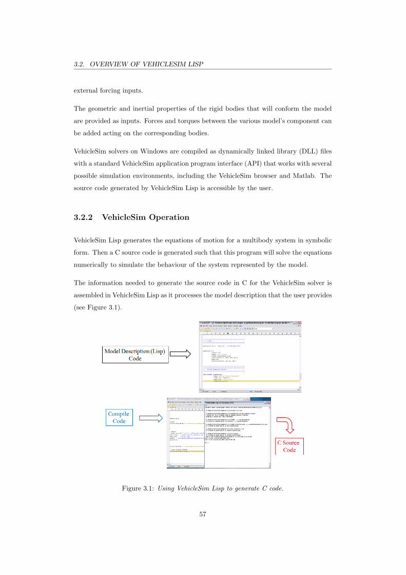
3.2. OVERVIEW OF VEHICLESIM LISP
external forcing inputs.
The geometric and inertial properties of the rigid bodies that will conform the model
are provided as inputs. Forces and torques between the various model’s component can
be added acting on the corresponding bodies.
VehicleSim solvers on Windows are compiled as dynamically linked library (DLL) files
with a standard VehicleSim application program interface (API) that works with several
possible simulation environments, including the VehicleSim browser and Matlab. The
source code generated by VehicleSim Lisp is accessible by the user.
3.2.2 VehicleSim Operation
VehicleSim Lisp generates the equations of motion for a multibody system in symbolic
form. Then a C source code is generated such that this program will solve the equations
numerically to simulate the behaviour of the system represented by the model.
The information needed to generate the source code in C for the VehicleSim solver is
assembled in VehicleSim Lisp as it processes the model description that the user provides
(see Figure 3.1).
Figure 3.1: Using VehicleSim Lisp to generate C code.
57
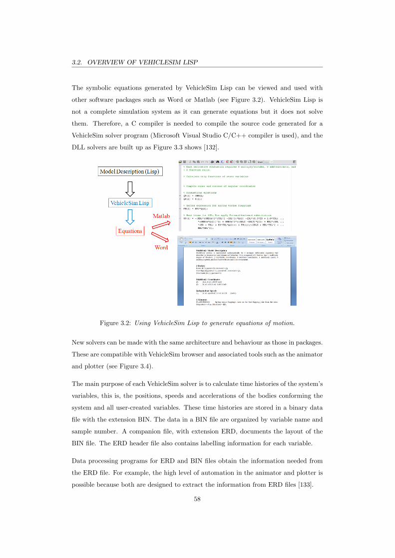
3.2. OVERVIEW OF VEHICLESIM LISP
The symbolic equations generated by VehicleSim Lisp can be viewed and used with
other software packages such as Word or Matlab (see Figure 3.2). VehicleSim Lisp is
not a complete simulation system as it can generate equations but it does not solve
them. Therefore, a C compiler is needed to compile the source code generated for a
VehicleSim solver program (Microsoft Visual Studio C/C++ compiler is used), and the
DLL solvers are built up as Figure 3.3 shows [132].
Figure 3.2: Using VehicleSim Lisp to generate equations of motion.
New solvers can be made with the same architecture and behaviour as those in packages.
These are compatible with VehicleSim browser and associated tools such as the animator
and plotter (see Figure 3.4).
The main purpose of each VehicleSim solver is to calculate time histories of the system’s
variables, this is, the positions, speeds and accelerations of the bodies conforming the
system and all user-created variables. These time histories are stored in a binary data
file with the extension BIN. The data in a BIN file are organized by variable name and
sample number. A companion file, with extension ERD, documents the layout of the
BIN file. The ERD header file also contains labelling information for each variable.
Data processing programs for ERD and BIN files obtain the information needed from
the ERD file. For example, the high level of automation in the animator and plotter is
possible because both are designed to extract the information from ERD files [133].
58
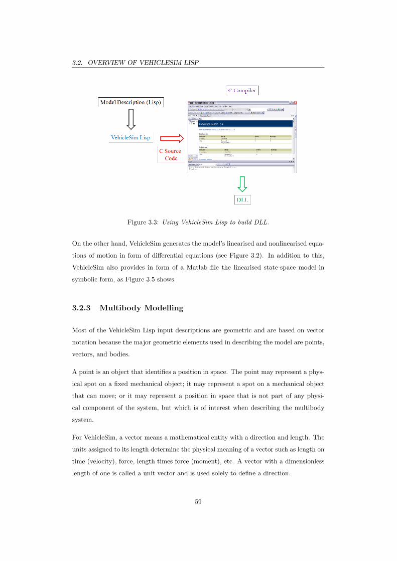
3.2. OVERVIEW OF VEHICLESIM LISP
Figure 3.3: Using VehicleSim Lisp to build DLL.
On the other hand, VehicleSim generates the model’s linearised and nonlinearised equa-
tions of motion in form of differential equations (see Figure 3.2). In addition to this,
VehicleSim also provides in form of a Matlab file the linearised state-space model in
symbolic form, as Figure 3.5 shows.
3.2.3 Multibody Modelling
Most of the VehicleSim Lisp input descriptions are geometric and are based on vector
notation because the major geometric elements used in describing the model are points,
vectors, and bodies.
A point is an object that identifies a position in space. The point may represent a phys-
ical spot on a fixed mechanical object; it may represent a spot on a mechanical object
that can move; or it may represent a position in space that is not part of any physi-
cal component of the system, but which is of interest when describing the multibody
system.
For VehicleSim, a vector means a mathematical entity with a direction and length. The
units assigned to its length determine the physical meaning of a vector such as length on
time (velocity), force, length times force (moment), etc. A vector with a dimensionless
length of one is called a unit vector and is used solely to define a direction.
59
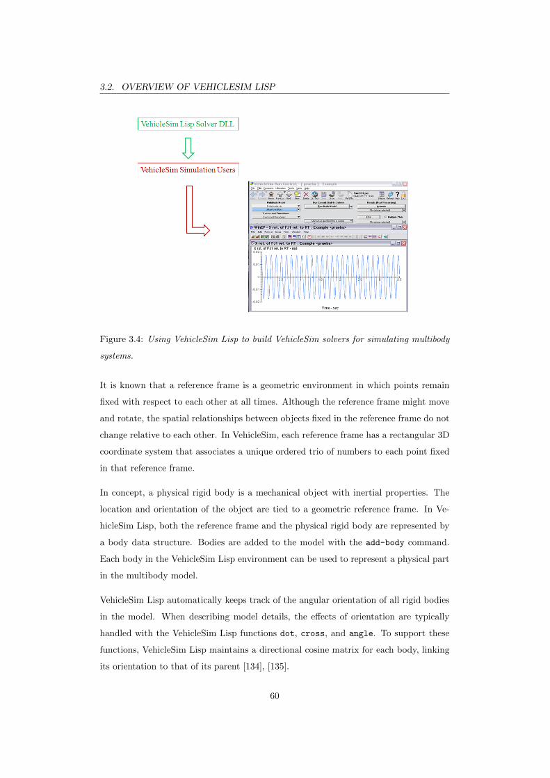
3.2. OVERVIEW OF VEHICLESIM LISP
Figure 3.4: Using VehicleSim Lisp to build VehicleSim solvers for simulating multibody
systems.
It is known that a reference frame is a geometric environment in which points remain
fixed with respect to each other at all times. Although the reference frame might move
and rotate, the spatial relationships between objects fixed in the reference frame do not
change relative to each other. In VehicleSim, each reference frame has a rectangular 3D
coordinate system that associates a unique ordered trio of numbers to each point fixed
in that reference frame.
In concept, a physical rigid body is a mechanical object with inertial properties. The
location and orientation of the object are tied to a geometric reference frame. In Ve-
hicleSim Lisp, both the reference frame and the physical rigid body are represented by
a body data structure. Bodies are added to the model with the add-body command.
Each body in the VehicleSim Lisp environment can be used to represent a physical part
in the multibody model.
VehicleSim Lisp automatically keeps track of the angular orientation of all rigid bodies
in the model. When describing model details, the effects of orientation are typically
handled with the VehicleSim Lisp functions dot, cross, and angle. To support these
functions, VehicleSim Lisp maintains a directional cosine matrix for each body, linking
its orientation to that of its parent [134], [135].
60
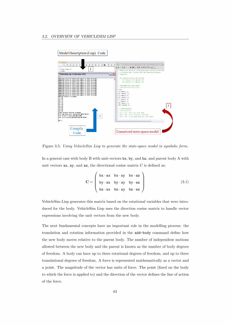
3.2. OVERVIEW OF VEHICLESIM LISP
Figure 3.5: Using VehicleSim Lisp to generate the state-space model in symbolic form.
In a general case with body B with unit-vectors bx, by, and bz, and parent body A with
unit vectors ax, ay, and az, the directional cosine matrix C is defined as:
C =
bx · ax bx · ay bx · az
by · ax by · ay by · az
bz · ax bz · ay bz · az
(3.1)
VehicleSim Lisp generates this matrix based on the rotational variables that were intro-
duced for the body. VehicleSim Lisp uses the direction cosine matrix to handle vector
expressions involving the unit vectors from the new body.
The next fundamental concepts have an important role in the modelling process: the
translation and rotation information provided in the add-body command define how
the new body moves relative to the parent body. The number of independent motions
allowed between the new body and the parent is known as the number of body degrees
of freedom. A body can have up to three rotational degrees of freedom, and up to three
translational degrees of freedom. A force is represented mathematically as a vector and
a point. The magnitude of the vector has units of force. The point (fixed on the body
to which the force is applied to) and the direction of the vector defines the line of action
of the force.
61
3.3. VEHICLESIM CHARACTERISTICS
Other fundamental concept used in VehicleSim is the moment; it is always defined
relative to a point, such that the distance vector in the moment expression is the position
vector connecting the reference point for the moment with any point lying on the line
of action of the force [134], [135].
3.3 VehicleSim Characteristics
The purpose of the VehicleSim solver is to solve the dynamical equations of motion to
calculate the time histories of the variables contained in the mathematical model that
represent the system’s variables.
3.3.1 State Variables
VehicleSim Lisp introduces the state variables needed to describe the moving reference
frames, and uses them as needed to develop mathematical expressions of variables that
represent the equations of motion of the system under study. The state variables for
a VehicleSim multibody system are divided into two sets: generalized coordinates and
generalized speeds.
The generalized coordinates are the variables involving angular and translational dis-
placements. The set of generalized coordinates is defined such that it is possible to
reconstruct the position of any point in any part in the system. VehicleSim Lisp can
derive expressions for the absolute coordinates of any point located on any mechanical
part using the generalized coordinates and dimensional parameters. On the other hand,
a set of generalized speeds complements the set of generalized coordinates, by adding
the capability for VehicleSim Lisp to determine the velocity vector of any point located
on any part in the multibody system.
From the user point of view, the set of state variables also includes variables that are
not defined by differential equations, but whose values are, nevertheless, required to
fully define the current state of the model. However, in VehicleSim environment, the
term ”state variables” usually refers only to variables that are defined by differential
equations.
62
3.3. VEHICLESIM CHARACTERISTICS
The add-variables command is used to include one or more variables in the coded
program and to declare that they are not constant during a run [134].
Controlling the Definition of the State Variables
State variables are introduced automatically when the command add-body is used to
define a body that can move relative to its parent. One generalized coordinate is in-
troduced for each degree of freedom of the new body relative to its parent, and the
coordinates are the amplitudes of the permitted movements. The equations of mo-
tion for a system involve a minimum number of coordinates and a speed variable is
introduced automatically with each coordinate. The speed variable is defined as the
derivative of the coordinate, except for the following three cases [134]:
• A body with three rotational degrees of freedom relative to its parent has three
rotational speed variables defined as scalar measures of the absolute rotational
velocity of the body.
• A body with three translational degrees of freedom relative to its parent has three
translational speed variables defined as scalar measures of the absolute velocity of
the body mass center.
• A body restricted to planar motions, with two translational degrees of freedom
has the translational speeds defined as scalar measures of the absolute velocity of
the body mass center.
3.3.2 Equations of Motion
VehicleSim can provide pure kinematical analyses and simulation in quasi-static equilib-
rium conditions. In these cases, values of the state variables are obtained as functions of
time. The majority of equations produced by VehicleSim Lisp are arithmetic statements
that define the output variables and the derivatives of the state variables [134].
63

3.3. VEHICLESIM CHARACTERISTICS
Dynamic System Simulation
The form of simulation generated by VehicleSim Lisp is one in which the system responds
dynamically to specified inputs. The number of degrees of freedom of the multibody
system model is the minimal number of independent generalized speeds needed to define
the absolute velocity vector of any point on any body in the system.
During the simulation the generalized coordinates are computed by numerical integra-
tion of a set of ordinary differential equations of the form:
q = s (3.2)
where q is an array of the derivatives of the generalized coordinates, and s is an array of
speeds defined in terms of the current values of the state variables and known functions
of time. The equation (3.2) defines the geometric relationships between the generalized
coordinates and generalized speeds.
u = f (3.3)
u is an array of the derivatives of the generalized speeds, and f is an array whose
elements are computed from the current values of the state variables and time.
The equations (3.3) are developed by VehicleSim Lisp such that they: a) are independent
and b) satisfy Newton’s second law and Euler’s equations. In vector form, Newton’s
second law for a rigid body is: ∑f =
dp
dt= ma (3.4)
where∑f is the vector sum of all forces acting on the body, p is the vector momentum
of the body, m is the body mass, and a is the vector acceleration of the mass centre of
the body. The vector form of Euler’s equations for a rigid body is:
∑t =
dh
dt= I · α+ ω × I · ω (3.5)
where∑t is the vector sum of all torques and moments acting on the body about its
mass centre, h is the vector angular momentum of the body about its mass centre, I
is the inertia dyadic of the body relative to its mass centre, α is the vector angular
acceleration of the body, and ω is the vector angular velocity of the body.
64
3.3. VEHICLESIM CHARACTERISTICS
A dynamical simulation program computes the state variables (generalized coordinates
and generalized speeds) by numerically integrating equations (3.2) and (3.3).
The mathematical model might use numerical methods to solve a set of nonlinear al-
gebraic equations that implicitly define some variables that are similar to generalized
coordinates because they define locations or orientations of rigid bodies in the system.
In addition to this, coordinate variables that are calculated directly are called computed
coordinates. They are calculated by applying simple arithmetic statements, if it is re-
quired. They are computed numerically by using the Newton-Raphson iteration method
[134].
Kinematics
A kinematical model has no dynamical degree of freedom, and therefore, no generalized
speeds. In most cases, a kinematical simulation does not involve differential equations.
Generalized coordinates used to describe positions of points are all either explicit func-
tions of time or dependent computed coordinates that are computed on the basis of
algebraic equations [134].
3.3.3 Numerical Solution
The purpose of the solver program produced by VehicleSim Lisp (VehicleSim-Browser)
is to compute the output variables at intervals of time as the simulation is being carried
out. The output variables are defined by solving the dynamical equations of motion
containing the state variables.
There are four classes of computation methods that might be used by in a VehicleSim
solver program.
• Simple arithmetic statements.
• Numerical integration of a set of ordinary differential equations.
• Solution of a set of simultaneous linear algebraic equations.
• Solution of a set of simultaneous nonlinear algebraic equations.
65
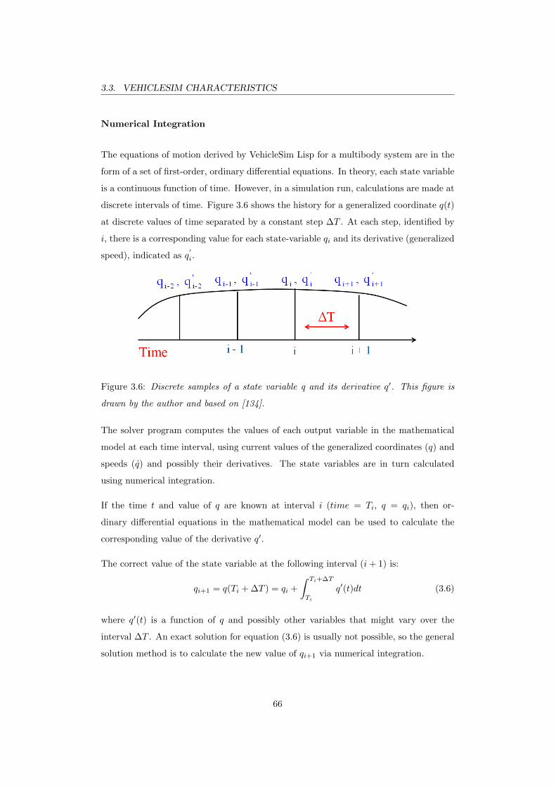
3.3. VEHICLESIM CHARACTERISTICS
Numerical Integration
The equations of motion derived by VehicleSim Lisp for a multibody system are in the
form of a set of first-order, ordinary differential equations. In theory, each state variable
is a continuous function of time. However, in a simulation run, calculations are made at
discrete intervals of time. Figure 3.6 shows the history for a generalized coordinate q(t)
at discrete values of time separated by a constant step ∆T . At each step, identified by
i, there is a corresponding value for each state-variable qi and its derivative (generalized
speed), indicated as q′
i.
Figure 3.6: Discrete samples of a state variable q and its derivative q′. This figure is
drawn by the author and based on [134].
The solver program computes the values of each output variable in the mathematical
model at each time interval, using current values of the generalized coordinates (q) and
speeds (q) and possibly their derivatives. The state variables are in turn calculated
using numerical integration.
If the time t and value of q are known at interval i (time = Ti, q = qi), then or-
dinary differential equations in the mathematical model can be used to calculate the
corresponding value of the derivative q′.
The correct value of the state variable at the following interval (i+ 1) is:
qi+1 = q(Ti + ∆T ) = qi +
∫ Ti+∆T
Ti
q′(t)dt (3.6)
where q′(t) is a function of q and possibly other variables that might vary over the
interval ∆T . An exact solution for equation (3.6) is usually not possible, so the general
solution method is to calculate the new value of qi+1 via numerical integration.
66
3.3. VEHICLESIM CHARACTERISTICS
Euler integration methodology does not account for any change in the derivatives over
the time interval and is not accurate unless ∆T is small and changes in the derivative
are negligible over the step [134].
Solution of Simultaneous Algebraic Equations
It is assumed that there is a set of n equations for independent variables x1, x2, ..., xn
in column vector x with the form:
g1(x1, x2, ...xn) = 0
g2(x1, x2, ...xn) = 0
....
gn(x1, x2, ...xn) = 0
(3.7)
These equations are written in vector form as:
g(x, t) = 0 (3.8)
where t is the time.
If the equations are independent, then there might be enough information to solve for
the variables x if the number of equations equals the number of variables. There are
two solution methods used in VehicleSim solver programs, depending on whether the
equations are linear or nonlinear.
Linear Algebraic Equations
Linear equations are given in the form:
Ax = b (3.9)
where A is an n×n matrix and b is an column vector of length n. The elements of A and
b can be complicated to calculate, and can include nonlinear functions. Nevertheless, if
they do not involve any of the elements of x, then the equations are linear in x. The
solution in this linear case is of the form:
67
3.3. VEHICLESIM CHARACTERISTICS
x = A−1b (3.10)
A more efficient solution is the Lower-Upper triangular Decomposition (LUD). The
matrix A is written as a product of two matrices, L and U , such that L has a lower-
triangular form, and U has an upper-triangular form. The equation set can then be
written in the form:
Ax = (LU)x = L(Ux) = b (3.11)
and equation (3.11) can be written as two equation sets:
Ly = b (3.12)
Ux = y (3.13)
The advantage of the above form is that triangular sets of equations can be solved by
sequential substitution. Solution of linear equations by LUD methodology involves two
steps: a) the original A matrix is decomposed into L− U form. This is normally done
such that the values of L and U matrices occupy the computer storage space originally
used to hold the elements of the A matrix. (Values that are defined as always being
zero or one are not stored). Equations (3.12) and (3.13) are solved in the second step
by forward and backward substitution.
Most multibody mathematical models will include sets of simultaneous linear algebraic
equations. In most cases, VehicleSim Lisp solves those sets of equations by applying the
LUD method symbolically [134].
Nonlinear Algebraic Equations
Nonlinear algebraic equations can be expressed as:
g(x, t) = 0 (3.14)
They can be solved iteratively if: a) a solution exists, b) an initial guess is provided for
x that is reasonably close to the right solution. Newton-Raphson method is used when
needed in VehicleSim solver programs. This method is based in a sequence of steps as
follows:
68
3.4. BUILDING A MODEL
• provided guesses values for [x1, x2, ..., xn]T = x(i), where the index i is the itera-
tion number.
• compute −gi i.e., iteration. If all |gj | < ε with j = 1, ..., n (j is the subscript
iteration) and ε is an error threshold, then stop. The solution is xi. Otherwise,
continue.
• Compute the Jacobian matrix Ji, where each element is defined as:
(Jj,k)i =
(∂gj∂xk
)i
(3.15)
• Solve for ∆xi using the LUD method and equation set: Ji∆xi = −gi
• Update the best guess of solution: xi+1 ← xi + ∆xi
• Increment i (i← i+ 1), then go to second step.
When the Newton-Raphson iteration is used in a VehicleSim solver, the VehicleSim Lisp
derives the elements of the Jacobian matrix symbolically and writes a C function that
calculates the matrix based on the current values of the state variables [134].
3.4 Building a Model
When writing up the code for building a VehicleSim model certain order in which the
commands appear is usually followed. In general, at the head of a VehicleSim program
there are certain commands that are used to reset the system, define the gravitational
field, select the unit system to be used, the possible linearization of equations of motion,
etc. When the analyst does not exercise choice overtly in these matters, default settings
come from a configuration file that the analyst is free to access.
VehicleSim Lisp in general follows the modelling sequence as shown in Figure 3.7. Ve-
hicleSim commands are used to describe the components of a multibody system in a
parent-child relationship according to their physical constraints and joints. As it can
be seen in Figure 3.7, the commands incorporate and describe in sequential manner the
69

3.4. BUILDING A MODEL
Figure 3.7: VehicleSim commands main sequence. This figure is done by the author and
based on [134].
rigid bodies that conform the system, the corresponding physical values such as name,
mass, inertia, the rotations amongst others, are also included.
A VehicleSim program begins with an inertial reference frame n, with fixed origin, no,
and fixed directions [nx], [ny] and [nz] already defined. As new bodies are added to
the system, having freedoms relative to n, local origins and axes are defined.
The code can transform from local coordinates to global ones and vice versa. Points
specified globally are conveniently used to define points in bodies. The body fixed
points coincide with the corresponding global points, fixed in n, when the system is on
its nominal configuration. Most points are fixed in bodies but a point may be defined
as moving with its location in a body determined by its specified coordinates. This is
especially useful for describing time varying contact points between two bodies.
The main commands used to build a multibody model are briefly described as follows:
• add-gravity
This command defines a uniform gravitational field, its direction. If not specified
with the keyword :direction, it is set to nz as in VehicleSim the direction along
the Z axis positive in down direction. nz is the unit vector in n. As it was
mentioned before, n is the inertial reference frame.
70

3.4. BUILDING A MODEL
• add-point
This command defines a point that can later be used for describing forces, etc.
The required argument symbol is used to identify the point at a later stage.
• add-body
This command defines a rigid body, its coordinate system, its mass properties,
and the kinematics of a joint connecting it to another body that is already in the
model. The existing body used as a reference for the new body is called the parent
of the new body, which is recalled as the child.
The add-body command has one required argument, symbol, used to identify the
new body in all future references and to generate symbols for parameters and
points associated with this new body.
• add-line-force
This command defines a force in the system that passes through a given point and
whose line of action has a specified direction. The required argument, symbol, is
a ”symbol” used later to identify the force.
• add-moment
This command introduces a moment between two bodies. The required argument
is a symbol used to identify the moment. Note that at least one of the optional
arguments body1 or body2 must be included in order for the moment to act.
• add-speed-constraint
It is an algebraic expression that is identically zero when the constraint is satisfied.
The optional argument u is a generalized speed that is eliminated by the constraint.
If u is not provided, then add-speed-constraint uses some programmed criteria
to select one automatically [134], [135].
71

3.5. CHAPTER SUMMARY
3.5 Chapter Summary
In this chapter the main characteristics, properties and commands of VehicleSim Lisp
that will be used in this work have been introduced and briefly described.
The general properties and operation conditions of VehicleSim were presented in sec-
tion 3.2.1 and 3.2.2. Section 3.2.3 explains in detail the fundamental characteristics of
VehicleSim Lisp as multibody software. Section 3.3 has been provided an overview of
the numerical methods that VehicleSim uses. Finally, section 3.4 contains and describes
the main sequence of VehicleSim commands that are used in the modelling process in
this work.
In the following chapters, a specific type of helicopter will be modelled following the
general program structure described in here. It will be shown how by using VehicleSim,
systems conformed of rigid bodies can be modelled and the convenience of this approach
with respect to other modelling tools in terms of reduced complexity of the program,
reduced computing time and possibility of modifying the model without the need of
building it again.
72
Part II
Helicopter Models
73
Chapter 4
Caliber 3 Dynamic Model
4.1 Introduction
Unmanned Aerial Vehicles have existed for many decades; in fact, various type of drones
have been used since World War I. In the previous decade, the development, procure-
ment and deployment of UAVs for military applications rapidly expanded. These days,
the use of Unmanned Aerial Vehicle (UAV) is growing in the private and civil sectors,
due to their ability for forest fire fighting, emergency mountain rescue, climate mon-
itoring, aerial photography, mapping and surveying, etc. A wide range of UAVs are
used by the police and civil security for law enforcement as well as border security and
coastguard surveillance. These machines are designed to perform surveillance tasks,
typically carrying cameras and other type of sensors.
Small unmanned aerial rotorcrafts have two main features that make them very useful.
First, small UAVs are designed to be carried by either a single man, or transported
with a vehicle, without the need of dedicated loading equipment. Second, unmanned
rotorcrafts have a vertical take off, landing and hovering capabilities. They do not
require a runway, a launching device or a dedicated recovery system and can easily hold
their position when required [136].
The purpose of this chapter is to model a particular type of Unmanned Aerial Vehicle by
using VehicleSim, showing as other subsystems are as well implemented, the elevators
74

4.2. CALIBER 3 DESCRIPTION AND PARAMETERS IDENTIFICATION
and the swashplate. The modelling process is similar to the one will describe in the
following chapter, whereas the dimensions, the physical parameters such as fuselage’s
mass, blades’ masses amongst others, do differ from the following case. First, a general
overview of the UAV prototype under study (Caliber 3) is given. This is followed by
modelling the details and a description of the multibody model in VehicleSim and,
finally some results from the simulations carried out are shown.
The work carried out in this chapter was performed under the umbrella of a joint project
between The City University London and the La Laguna University, Spain: ”DPI2010-
20751-C02-02. Diseno de estrategias inteligentes de control y diagnostico basadas en el
analisis de vibraciones: Aplicacion a helicopteros no tripulados UAV’s” granted by the
Innovation and Science Ministry (Spain).
At City University the model was implemented in VehicleSim, vibrations were generated
on the main rotor in order to detect their impact on the fuselage. After that, the La
Laguna University team developed strategies of control based in artificial intelligence
methods in order to reduce the effects of these vibrations on the fuselage, and potentially
improve in this way the quality of images obtained by the UAV’s onboard vision system.
As a result of this work, a journal paper was published ([128]).
4.2 Caliber 3 Description and Parameters Identifica-
tion
The physical prototype of the model under study is shown in Figure 4.1. It is a radio
controlled engine helicopter, Caliber 3 [139].
The engine is a KYOSHO GX36H for helicopter and it has a radio for engine-powered
R/C helicopter (see Figure 4.2).
As it can be seen in Figure 4.1, the helicopter consists in three main subsystems: main
rotor, fuselage and tail rotor, the fuselage in this case contains a fuel tank.
The initial design of the VehicleSim model of the Caliber 3 was approached from a
dynamics-only perspective. The physical properties such as weight, fuselage’s mass,
blades’ masses amongst others, were measured at La Laguna University. Other impor-
75
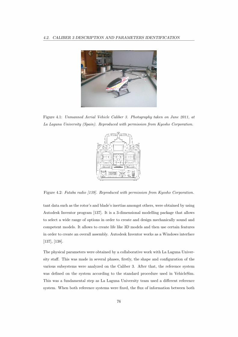
4.2. CALIBER 3 DESCRIPTION AND PARAMETERS IDENTIFICATION
Figure 4.1: Unmanned Aerial Vehicle Caliber 3. Photography taken on June 2011, at
La Laguna University (Spain). Reproduced with permission from Kyosho Corporation.
Figure 4.2: Futaba radio [139]. Reproduced with permission from Kyosho Corporation.
tant data such as the rotor’s and blade’s inertias amongst others, were obtained by using
Autodesk Inventor program [137]. It is a 3-dimensional modelling package that allows
to select a wide range of options in order to create and design mechanically sound and
competent models. It allows to create life like 3D models and then use certain features
in order to create an overall assembly. Autodesk Inventor works as a Windows interface
[137], [138].
The physical parameters were obtained by a collaborative work with La Laguna Univer-
sity staff. This was made in several phases, firstly, the shape and configuration of the
various subsystems were analyzed on the Caliber 3. After that, the reference system
was defined on the system according to the standard procedure used in VehicleSim.
This was a fundamental step as La Laguna University team used a different reference
system. When both reference systems were fixed, the flux of information between both
76
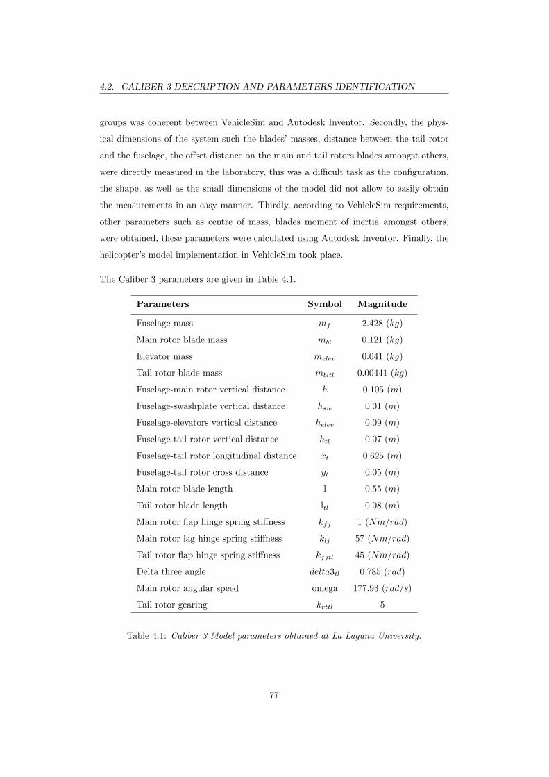
4.2. CALIBER 3 DESCRIPTION AND PARAMETERS IDENTIFICATION
groups was coherent between VehicleSim and Autodesk Inventor. Secondly, the phys-
ical dimensions of the system such the blades’ masses, distance between the tail rotor
and the fuselage, the offset distance on the main and tail rotors blades amongst others,
were directly measured in the laboratory, this was a difficult task as the configuration,
the shape, as well as the small dimensions of the model did not allow to easily obtain
the measurements in an easy manner. Thirdly, according to VehicleSim requirements,
other parameters such as centre of mass, blades moment of inertia amongst others,
were obtained, these parameters were calculated using Autodesk Inventor. Finally, the
helicopter’s model implementation in VehicleSim took place.
The Caliber 3 parameters are given in Table 4.1.
Parameters Symbol Magnitude
Fuselage mass mf 2.428 (kg)
Main rotor blade mass mbl 0.121 (kg)
Elevator mass melev 0.041 (kg)
Tail rotor blade mass mbltl 0.00441 (kg)
Fuselage-main rotor vertical distance h 0.105 (m)
Fuselage-swashplate vertical distance hsw 0.01 (m)
Fuselage-elevators vertical distance helev 0.09 (m)
Fuselage-tail rotor vertical distance htl 0.07 (m)
Fuselage-tail rotor longitudinal distance xt 0.625 (m)
Fuselage-tail rotor cross distance yt 0.05 (m)
Main rotor blade length l 0.55 (m)
Tail rotor blade length ltl 0.08 (m)
Main rotor flap hinge spring stiffness kfj 1 (Nm/rad)
Main rotor lag hinge spring stiffness klj 57 (Nm/rad)
Tail rotor flap hinge spring stiffness kfjtl 45 (Nm/rad)
Delta three angle delta3tl 0.785 (rad)
Main rotor angular speed omega 177.93 (rad/s)
Tail rotor gearing krttl 5
Table 4.1: Caliber 3 Model parameters obtained at La Laguna University.
77
4.3. MODEL DESCRIPTION
4.3 Model Description
Multibody systems can be modelled in various ways, one of them is the combination of
several interacting subsystems. The main aim of this section is to implement a model
of an UAV as a multibody system with several subsystems as well as several constrains
between the different degrees of freedom. VehicleSim allows to develop other technical
considerations in the modelling process, for example, the elevators can be modelled by
imposing restrictions. The general considerations taken into account for the modelling
process are described in the following lines:
• The helicopter is on Sikorsky configuration: this is, the main rotor is perpendicular
to the tail rotor. The axis of rotation of the tail rotor is transverse to the axis of
rotation of the main rotor. Both subsystems are mounted on the fuselage.
• The main rotor consists of two equally spaced blades as well as two elevators
pinned to a central hub. The blades have free motion in the plane of the disc and
this is allowed by the blade’s hinges.
• The tail rotor consists of two equally spaced blades joined to a secondary hub.
• The blades are rigid in both rotors.
• The angular speeds are implemented as constant parameters in both rotors and
there exists a proportional ratio between them.
• The main rotor’s hinges have three degrees of freedom: feather, lag and flap.
• The tail rotor hinges have two degrees of freedom: feather and flap.
• Feather-flap coupling effects are considered in the case of the tail rotor.
• The fuselage has six degrees of freedom: three translations along the corresponding
(X, Y , Z) axes and three rotations (ϕ, φ, ζ) around the same axes.
78
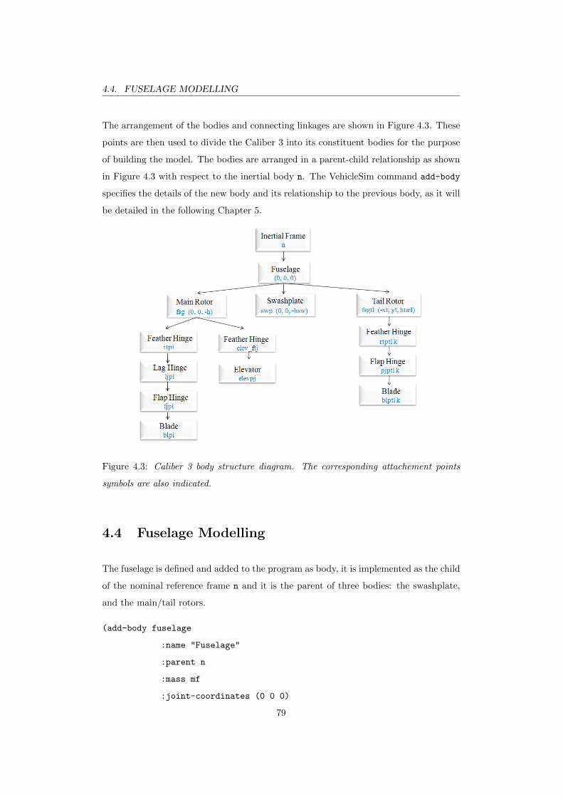
4.4. FUSELAGE MODELLING
The arrangement of the bodies and connecting linkages are shown in Figure 4.3. These
points are then used to divide the Caliber 3 into its constituent bodies for the purpose
of building the model. The bodies are arranged in a parent-child relationship as shown
in Figure 4.3 with respect to the inertial body n. The VehicleSim command add-body
specifies the details of the new body and its relationship to the previous body, as it will
be detailed in the following Chapter 5.
Figure 4.3: Caliber 3 body structure diagram. The corresponding attachement points
symbols are also indicated.
4.4 Fuselage Modelling
The fuselage is defined and added to the program as body, it is implemented as the child
of the nominal reference frame n and it is the parent of three bodies: the swashplate,
and the main/tail rotors.
(add-body fuselage
:name "Fuselage"
:parent n
:mass mf
:joint-coordinates (0 0 0)
79

4.5. SWASHPLATE AND MAIN ROTOR MODELLING
:translate (x y z)
:body-rotation-axes (z y x)
:parent-rotation-axis z
:reference-axis x
:inertia-matrix (Ifx Ify Ifz)
:cm-coordinates (xcmf ycmf zcmf))
The fuselage is added as a body with mass, moments of inertia as well as centre of mass.
It has translational degrees of freedom along the x, y and z directions of n, as n is its
parent. The yaw, pitch and roll rotational degrees of freedom around the axes z, y and
x are respectively considered in order to describe the full rotation of the helicopter in
the space.
As mentioned before, the helicopter structure is complex, the fuselage has a fuel tank,
besides the fuselage itself, the tail rotor is assembled with a mechanical connection as
well as the swashplate and the main rotor, being this structure a mesh of mechanical
connections.
4.5 Swashplate and Main Rotor Modelling
The modelling process of the Caliber 3 is similar to the helicopter model build up in the
following chapter. The main differences between both models are that the swashplate
is modelled here as new body and the elevators are now included and implemented on
the main rotor.
4.5.1 Swashplate Modelling
The blade feather angles can be mathematically described as a Fourier series. Blade
feather is mechanically induced from two sources:
• The helicopter control system uses a swashplate, the orientation of which is con-
trolled by the pilot. The control inputs produced by the swashplate consist of the
collective and cyclic feather angles. The collective feather controls the average
blade feather angle, therefore, the blade lift and the average total thrust. On the
80
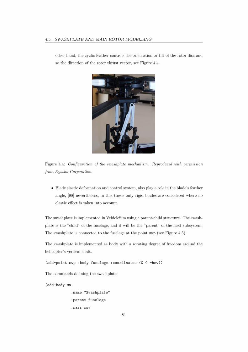
4.5. SWASHPLATE AND MAIN ROTOR MODELLING
other hand, the cyclic feather controls the orientation or tilt of the rotor disc and
so the direction of the rotor thrust vector, see Figure 4.4.
Figure 4.4: Configuration of the swashplate mechanism. Reproduced with permission
from Kyosho Corporation.
• Blade elastic deformation and control system, also play a role in the blade’s feather
angle, [98] nevertheless, in this thesis only rigid blades are considered where no
elastic effect is taken into account.
The swashplate is implemented in VehicleSim using a parent-child structure. The swash-
plate is the ”child” of the fuselage, and it will be the ”parent” of the next subsystem.
The swashplate is connected to the fuselage at the point swp (see Figure 4.5).
The swashplate is implemented as body with a rotating degree of freedom around the
helicopter’s vertical shaft.
(add-point swp :body fuselage :coordinates (0 0 -hsw))
The commands defining the swashplate:
(add-body sw
:name "Swashplate"
:parent fuselage
:mass msw
81
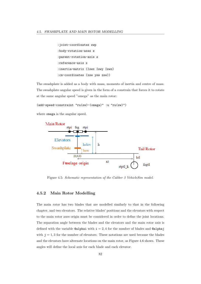
4.5. SWASHPLATE AND MAIN ROTOR MODELLING
:joint-coordinates swp
:body-rotation-axes z
:parent-rotation-axis z
:reference-axis x
:inertia-matrix (Iswx Iswy Iswz)
:cm-coordinates (xsw ysw zsw))
The swashplate is added as a body with mass, moments of inertia and centre of mass.
The swashplate angular speed is given in the form of a constrain that forces it to rotate
at the same angular speed ”omega” as the main rotor:
(add-speed-constraint "ru(sw)-(omega)" :u "ru(sw)")
where omega is the angular speed.
Figure 4.5: Schematic representation of the Caliber 3 VehicleSim model.
4.5.2 Main Rotor Modelling
The main rotor has two blades that are modelled similarly to that in the following
chapter, and two elevators. The relative blades’ positions and the elevators with respect
to the main rotor axes origin must be considered in order to define the joint locations.
The separation angle between the blades and the elevators and the main rotor axis is
defined with the variable @alphai with i = 2, 4 for the number of blades and @alphaj
with j = 1, 3 for the number of elevators. These notations are used because the blades
and the elevators have alternate locations on the main rotor, as Figure 4.6 shows. These
angles will define the local axis for each blade and each elevator.
82
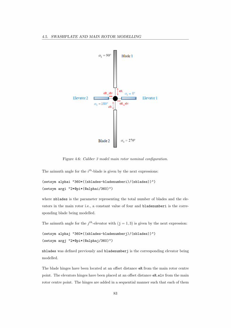
4.5. SWASHPLATE AND MAIN ROTOR MODELLING
Figure 4.6: Caliber 3 model main rotor nominal configuration.
The azimuth angle for the ith-blade is given by the next expressions:
(setsym alphai "360*((nblades-bladenumberi)/(nblades))")
(setsym argi "2*@pi*(@alphai/360)")
where nblades is the parameter representing the total number of blades and the ele-
vators in the main rotor i.e., a constant value of four and bladenumberi is the corre-
sponding blade being modelled.
The azimuth angle for the jth-elevator with (j = 1, 3) is given by the next expression:
(setsym alphaj "360*((nblades-bladenumberj)/(nblades))")
(setsym argj "2*@pi*(@alphaj/360)")
nblades was defined previously and bladenumberj is the corresponding elevator being
modelled.
The blade hinges have been located at an offset distance eR from the main rotor centre
point. The elevators hinges have been placed at an offset distance eR elv from the main
rotor centre point. The hinges are added in a sequential manner such that each of them
83
4.5. SWASHPLATE AND MAIN ROTOR MODELLING
is the child of the previous one and the parent of the following hinge.
The blades’ offset positions are defined as two variables xi, yi:
(setsym xi "eR*sin(@argi)")
(setsym yi "eR*cos(@argi)")
The angles argi are used to define the local axis for each blade as biaxesx, biaxesy
and biaxesz. The blades’ local axes are defined in terms of the inertial reference axes.
The position of each blade with respect to the main rotor is determined as:
(setsym biaxesx "-sin(@argi)*[rty]+cos(@argi)*[rtx]")
(setsym biaxesy "sin(@argi)*[rtx]+cos(@argi)*[rty]")
(setsym biaxesz "[rtz]")
The locations of the elevators offset are represented by the variables xj, yj:
(setsym xj "eR elv*sin(@argj)")
(setsym yj "eR elv*cos(@argj)")
The angles argj are used to define the local axis for each elevator as bjaxesx, bjaxesy
and bjaxesz. Therefore, the local axes for the elevators are implemented in terms of
the inertial reference axes. The position of each elevator with respect to the main rotor
is given as:
(setsym bjaxesx "-sin(@argj)*[rty]+cos(@argj)*[rtx]")
(setsym bjaxesy "sin(@argj)*[rtx]+cos(@argj)*[rty]")
(setsym bjaxesz "[rtz]")
The rotor is connected to the fuselage at the point fsg (see Figure 4.5) using a similar
parent-children structure:
(add-point fsg :body fuselage :coordinates (0 0 -h))
(add-body rt
:name "Rotor"
:parent fuselage
:mass mrt
:joint-coordinates fsg
:body-rotation-axes z
84
4.5. SWASHPLATE AND MAIN ROTOR MODELLING
:parent-rotation-axis z
:reference-axis x
:inertia-matrix (Irtx Irty Irtz)
:cm-coordinates (xcmrt ycmrt zcmrt))
The rotor is set up as a body with mass, moments of inertia as well as centre of mass.
The rotational degree of freedom around the axes Z is allowed.
The different degrees of freedom are added on the blades is a sequential manner where
each of them is the child of the previous one. The hinges are connected to the main
rotor, at the points rtpi, where i = 2, 4. (Figure 4.5).
The blades hinges are also connected to the main rotor, at the point rtpi with i = 2, 4.
Various points in the helicopter nominal configuration within the coordinate system of
body n need to be defined because the feather will be connected as a subsequent degree
of freedom as well as the lag and flap. The blades will be connected to the last of these
points.
Thus, the main rotor nominal configuration is built in a sequential manner:
(add-point p nblabes i :body n :coordinates ("@xi" "@yi" -h))
the variables @xi and @yi were previusly defined.
(add-point rtpi :body rt :coordinates p nblabes i)
The feather hinge is connected to the main rotor at the point rtpi:
(add-body pji
:name "i-th Feather Joint"
:parent rt
:joint-coordinates rtpi
:body-rotation-axes y
:parent-rotation-axis "@biaxesy"
:reference-axis "@biaxesz"
:inertia-matrix 0
:mass 0)
85

4.5. SWASHPLATE AND MAIN ROTOR MODELLING
Once the feather hinge is defined, the lag hinge is connected to the feather hinge at the
point ljpi as a child of the feather hinge:
(add-point ljpi :body pji :coordinates p nblabes i)
(add-body lji
:name "i-th Lag Joint"
:parent pji
:joint-coordinates ljpi
:body-rotation-axes z
:parent-rotation-axis z
:reference-axis "@biaxesx"
:inertia-matrix 0
:mass 0)
The flap hinge is added as the child of the lag hinge at the point fjpi being the parent
of the blade:
(add-point fjpi :body lji :coordinates p nblabes i)
(add-body fji
:name "i-th Flap Joint"
:parent lji
:joint-coordinates fjpi
:body-rotation-axes x
:parent-rotation-axis "@biaxesx"
:reference-axis "@biaxesy"
:inertia-matrix 0
:mass 0)
Now, the blade is added as the child of the flap hinge:
(add-point blpi :body fji :coordinates p nblabes i)
(add-body bli
:name "i-th Blade"
:parent fji
:mass mbli
86
4.5. SWASHPLATE AND MAIN ROTOR MODELLING
:joint-coordinates blpi
:inertia-matrix (Iblxi Iblyi Iblzi)
:cm-coordinates (xbli ybli zbli))
The elevators hinges are connected to the main rotor, at the points p elev j, where
j = 1, 3. (See Figure 4.5). Various points in the helicopter nominal configuration within
the coordinate system of body n as the feather and the elevators will be added to the
model to these points.
(add-point p elev j :body n :coordinates ("@xj" "@yj" -helev))
(add-point elev ftj :body rt :coordinates p elev j)
On the other hand, the elevator is connected to the main rotor at the point elevftj.
(add-body pj j
:name "j-th Feather Joint"
:parent rt
:joint-coordinates elev ftj
:body-rotation-axes y
:parent-rotation-axis "@bjaxesy"
:reference-axis "@bjaxesz"
:inertia-matrix 0
:mass 0)
The elevator is similarly added as:
(add-point elevpj :body pj j :coordinates p elev j)
(add-body elevj
:name "j-th Elevator Joint"
:parent pj j
:mass melevj
:joint-coordinates elevpj
:inertia-matrix (Ielevxj Ielevyj Ielevzj)
:cm-coordinates (xblelevj yblelevj zblelevj))
87
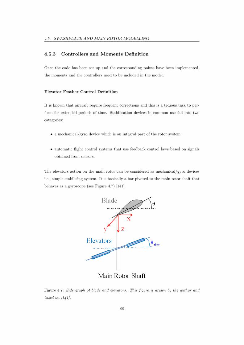
4.5. SWASHPLATE AND MAIN ROTOR MODELLING
4.5.3 Controllers and Moments Definition
Once the code has been set up and the corresponding points have been implemented,
the moments and the controllers need to be included in the model.
Elevator Feather Control Definition
It is known that aircraft require frequent corrections and this is a tedious task to per-
form for extended periods of time. Stabilisation devices in common use fall into two
categories:
• a mechanical/gyro device which is an integral part of the rotor system.
• automatic flight control systems that use feedback control laws based on signals
obtained from sensors.
The elevators action on the main rotor can be considered as mechanical/gyro devices
i.e., simple stabilising system. It is basically a bar pivoted to the main rotor shaft that
behaves as a gyroscope (see Figure 4.7) [141].
Figure 4.7: Side graph of blade and elevators. This figure is drawn by the author and
based on [141].
88
4.5. SWASHPLATE AND MAIN ROTOR MODELLING
The elevator is linked to the blade in such a manner that a tilt of the elevator relative
to the shaft introduces a change in the blades’ feather angle. As the elevator can pivot
relative to the shaft, its equation of motion on the same form as that of the blade under
the excitation of gyroscopic and inertia moments.
Let cl be the linkage ratio such that:
θ = clθelev (4.1)
θelev is the elevator’s angular displacement.
If cl is equal to one, one degree elevator tilt introduces one degree of blade feather.
Since the elevator does not affect the collective feather, equation (4.1) can be written
in the form [141]:
clθelev = −A1sinψ −B1cosψ (4.2)
where the cyclic pitch amplitudes A1 and B1 are functions of time and are given as:
B1 = cl
( qΩ
)ψ + cte (4.3)
ψ = Ωt, q is the rate of pitch and cte is an integration constant. A similar relationship
exists between the lateral cyclic pitch A1 and the rate of roll p.
A1 = cl
( pΩ
)ψ + cte (4.4)
In order to model the elevator’s feather angle, a PID controller needs to be defined. It
uses the variable @fhterror j, that it is defined as the input variable, and the output
is the moment applied to the feather hinge so that certain cyclic control is achieved.
Several variables need to be defined as well:
(setsym fhtpj j "rq(pjj)")
where j = 1, 3 and rq(pjj) specifies the angular position of the feather hinge with
respect to the main rotor.
The second variable, @afth j is the cyclic feather coefficient implemented as dictated
by equation (4.3):
89
4.5. SWASHPLATE AND MAIN ROTOR MODELLING
(setsym afth j "cl*(rq(fuselage,2)/omega)*omega*t+k1 inte")
cl and k1 inte are constant values, omega is the main rotor angular speed (see Table
4.1) and rq(fuselage,2) is the fuselage’s pitch rate of change.
The third introduced variable @bfth j, is the second feather coefficient (see equation
(4.4)):
(setsym bfth j "cl*(rq(fuselage,3)/omega)*omega*t+k2 inte")
k2 inte is a constant a value and rq(fuselage,3) is the fuselage’s roll rate of change.
Finally, the elevator’s cyclic feather @fht ref j, can be written as:
(setsym fht ref j "-@afth j*cos(omega*t)-@bfth j*sin(omega*t)")
where the coefficients afth j and bfth j previously described as variables, are used.
Now, the PID can be modelled:
(setsym fhterror j "@fhtiref j-@fhtpj j")
(add-state-variable ftq j ftqp j "F*L")
(set-aux-state-deriv ftqp j "kifht j*@fhterror j")
The command add-state-variable introduces a state variable for the moment expres-
sion that it is used to implement the elevator’s feather control. The integral part of the
moment control is defined by the set-aux-state-deriv command and uses the value
of the @fhterror j which is the tracking error.
This moment is applied between the fuselage and the elevator’s feather hinge.
(add-moment fhtc j
:name "pjctrl j"
:direction -[pjjy]
:body1 fuselage
:body2 pjj
:magnitude "ftq j+kfht j*(@fhterror j)+kdfht j*dxdt(@fhterror j)")
This controller uses the variable @fhterror j as the input, and the output is the moment
applied to the elevator feather hinge so that cyclic control is achieved. The parameters
kifht j, kfht j and kdfht j are the gains of the controller.
90
4.5. SWASHPLATE AND MAIN ROTOR MODELLING
The elevators rotate with opposite direction around of their local reference axes [pjjx,
pjjy, pjjz]. As a consequence of this, another moment needs to be considered on the
implementation of the second elevator.
Blade Feather Angle Control Implementation
The feather angle controller for each blade is defined in a similar way to the elevators
control. The variable @fht pj i is defined:
(setsym fht pj i "rq(pj i)")
where i = 2, 4 and rq(pj i) is the blades’ feather angular position with respect to the
main rotor.
The variable @fht ref is implemented as:
(setsym fht ref "fo-@afth j*cos(omega*t)-@bfth j*sin(omega*t)")
the coefficient fo describes the blades’ collective feather angle and the coefficients afth j
and bfth j describe the blades cyclic feather, keeping a ratio to the cyclic elevator
coefficients. The choice of these coefficients is dictated by the desired flight conditions.
fht ref is the Fourier series representation for the blade’s feather angle.
Now, some variables need to be defined before implemented a PID controller.
(setsym fht error i "@fht ref-@fht pj i")
(add-state-variable ft tq i ft tqp i "F*L")
(set-aux-state-deriv ft tqp i "kifht i*@fht error i")
The add-state-variable command introduces a state variable for the moment expres-
sion that it is used to implement the elevator’s feather control. The integral part of the
moment control is defined by the command set-aux-state-deriv and uses the value
of the variable @fhterror i defined above, being the tracking error.
This moment is applied between the swashplate and the blade feather.
91
4.5. SWASHPLATE AND MAIN ROTOR MODELLING
(add-moment fht c i
:name "pj ctrl i"
:direction -[pj iy]
:body1 sw
:body2 pj i
:magnitude "ft tq i+kfht i*(@fht error i)+kdfht i*dxdt(@fht error i)")
This controller uses the variable @fhterror i as the input, and the output is the mo-
ment applied to the blade feather hinge so that collective and cyclic controls are ade-
quately implemented. The parameters kifht i, kfht i and kdfht i are the gains of
the controller.
The blades rotate with opposite direction around of their local reference axes [pjix,
pjiy, pjiz]. As a consequence of this, another similar but opposite in sign moment
needs to be defined for the second blade.
Once that the fuselage, swashplate and the main rotor as well the elevators and blades
feather control have been modelled, the main rotor angular speed control also needs to
be implemented, being this task similar to the described in the following chapter, so its
process of implementation it is not included in here in order to avoid redundancy.
Moments Definition
The moments appearing on the main rotor (lag and flap moments respectively) are here
described: the lag hinges have a spring that introduces a force acting between the lag
hinge and the feather hinge, the spring stiffness is represented by the parameter klj.
The magnitude is given by Hooke’s Law:
(add-moment lagspringi
:name "i-th Lag Spring"
:body1 lji
:body2 pji
:magnitude "-klj*rq(lji)"
:direction [bliz])
and rq(lji) represents the angular displacement of the lag hinge.
92
4.6. TAIL ROTOR MODELLING
The flap hinges have a flap spring that introduces a spring force acting between the lag
hinge and the correspondent flap hinge (fji), the spring stiffness is represented by the
parameter kfj.
(add-moment flapspringi
:name "i-th Flap Spring"
:body1 fji
:body2 lji
:magnitude "-kfj*rq(fji)"
:direction [blix])
rq(fji) represents the angular displacement of the flap hinge. The magnitudes of the
flap and lag springs are indicated in Table 4.1.
4.6 Tail Rotor Modelling
The tail rotor modelling is implemented once the main rotor has been modelled. There
exist two main differences between the modelling of the main and tail rotors; there is
no modelled lag degree of freedom in the later case as there is no lag hinge on the
Caliber 3 tail rotor. On the contrary, there is feather-flap coupling via delta three angle
mechanism.
4.6.1 Bodies Definition
The tail rotor is built using a parent-child structure. First, the tail rotor is imple-
mented as the child of the fuselage, and then it is defined as the parent of the following
components. The tail rotor is connected to the fuselage at the point fsgtl:
(add-point fsgtl :body fuselage :coordinates (-xt yt htail))
(add-body tailrt
:name "Tail Rotor"
:parent fuselage
:mass mtailrt
:joint-coordinates fsgtl
93
4.6. TAIL ROTOR MODELLING
:body-rotation-axes y
:parent-rotation-axis y
:reference-axis z
:inertia-matrix (Irtlx Irtly Irtlz)
:cm-coordinates (xcmtl ycmtl zcmtl))
The tail rotor is set up as a body with mass, moments of inertia and centre of mass.
The rotational degree of freedom around the Y axes is considered. Note at this point
that the tail rotor rotation axes is perpendicular to the main rotor’s one. The coor-
dinates of the joint between the tail rotor and the fuselage are given by the command
:joint-coordinates, its numerical value is defined by the point fsgtl. Finally, its
moments of inertia are added in the last part of the modelling script.
The tail rotor has two blades, the relative blades’ positions with respect to the tail rotor
axes origin must be considered in order to define the joint locations. The separation
angle between the blades and the tail rotor axis is defined by the variable, @alphatlk,
being k = 1, .., n (n is the maximum number of blades).
The azimuth angle for each k-blade is given by:
(setsym alphatlk "360*((nblades tl-blade numberk tl)/(nblades tl))")
(setsym argk tl "2*@pi*(@alphatlk/360)")
where nblades tl is a parameter representing the total number of blades in the tail
rotor and, blade numberk tl is the corresponding blade being modelled.
All the blade hinges have been located at the same offset distance eRtl from the tail
rotor centre point.
The distance for each blade offset is defined as:
(setsym xk tl "eRtl*sin(@argk tl)")
(setsym zk tl "eRtl*cos(@argk tl)")
The angles @argk tl will be used to define the local axis for each blade (baxesxtl k,
baxesytl k, baxesztl k) are defined in terms of the inertial reference axes. Therefore,
it can be determined by using the blade’s position with respect to the tail rotor.
94
4.6. TAIL ROTOR MODELLING
A new set of local axes system is defined for each blade and its position with respect to
the tail rotor’s local axes ([tail rtx],[tail rty],[tail rtz]):
(setsym baxesxtl k "cos(@argk tl)*[tail rtx]+sin(@argk tl)*[tail rtz]")
(setsym baxesytl k "[tail rty]")
(setsym baxesztl k "-sin(@argk tl)*[tail rtx]+cos(@argk tl)*[tail rtz]")
A point in the helicopter nominal configuration within the coordinate system of body n
is defined because the feather hinge will be connected to it as well as a flap hinge. The
blade will be attached to this point.
The feather hinge is connected to the tail rotor at the point rtptl k where k = 1, 2.
The tail rotor nominal configuration can now be implemented:
(add-point ptl k1 :body n :coordinates ("-xt-@xk tl" yt "htail+@zk tl"))
(add-point rtptl k :body tailrt :coordinates ptl k1)
Each feather hinge is now included in the model with the following lines:
(add-body pjtl k
:name "k-th Feather Joint Tail"
:parent tailrt
:joint-coordinates rtptl k
:body-rotation-axes z
:parent-rotation-axis "@baxesztl k"
:reference-axis "@baxesxtl k"
:inertia-matrix 0
:mass 0)
It is a child of the tail rotor. Its mass is zero as well as the moment of inertia.
The flap hinge is connected to the feather hinge at the point pjptl k and it is the parent
of the blade and the child of the feather hinge:
(add-point ptl k2 :body n :coordinates ("-xt-@xk tl" yt "htail+@zk tl"))
(add-point pjptl k :body pjtl k :coordinates ptl k2)
95
4.6. TAIL ROTOR MODELLING
(add-body fjtl k
:name "k-th Flap Joint Tail"
:parent pjtl k
:joint-coordinates pjptl k
:body-rotation-axes x
:parent-rotation-axis "@baxesxtl k"
:reference-axis "@baxesytl k"
:inertia-matrix 0
:mass 0)
Finally, the tail rotor blades are added as flap hinges’ children:
(add-body bltl k
:name "k-th Blade Tail"
:parent fjtl k
:mass mbltl k
:joint-coordinates blptl k
:inertia-matrix (Iblxtl Iblytl Iblztl)
:cm-coordinates (xbltl ybltl zbltl))
The blades are added as bodies with mass, moments of inertia and centre of mass.
4.6.2 Controllers Implementation
In this section, the blades’ feather and flap dynamics are implemented under the action
of PID controllers. Details on how the implementation was carried out in VehicleSim
are provided in here.
4.6.3 Feather Control Definition
The tail rotor blades feather and delta three angle are modelled by using a PID con-
troller. This constrains the blades’ angular displacement with respect to the tail feather
axis ([tail rtz]).
The first line specifies the variable @ptlpj k as the first blade feather angular speed
as rq(pjtl k). Then, the variable @ptlref k is defined as the reference value for the
96
4.6. TAIL ROTOR MODELLING
collective feather angle, fotl, under the influence of the delta three angle on the blade’s
flap angle fjtl k.
(setsym ptlpj k "rq(pjtl k)")
(setsym ptlref k "fotl-tan(delta3tl)*rq(fjtl k)")
Next, a state variable is introduced for the torque that is used to control the blade’s
feather angle. The integral part of the torque is defined by the set-aux-state-deriv
and uses the error variable ptlerror k:
(setsym ptlerror k "@ptlref k-@ptlpj k")
(add-state-variable pltq k tptqp k "F*L")
(set-aux-state-deriv tptqp k "kiptl k*@ptlerror k")
The torque is applied between the tail rotor and the first blade’s feather hinge. This
controller uses the variable @ptlerror k as the input, and the output is the moment
applied to the first feather hinge so that satisfactory collective control is achieved. The
parameters kiptl k, kpptl k and kdptl k are the corresponding controller gains:
(add-moment ptlm k
:name "pjctl k"
:direction -[pjtlkz]
:body1 tailrt
:body2 pjtl k
:magnitude "pltq k+kpptl k*(@ptlerror k)+kdptl k*dxdt(@ptlerror k)")
The tail rotor mechanism forces the second blade to rotate around the Z axis in opposite
direction to the first tail blade, therefore, a second moment is considered on the tail
rotor and it is implemented in the similar manner to the previous one.
4.6.4 Flap Control Definition
In order to implement the tail rotor flap dynamics, a PID controller is designed; its
function is to maintain the flap angle since it is coupled to the feather angle by the
delta three angle:
97

4.6. TAIL ROTOR MODELLING
(setsym fltl k "rq(fjtl k)")
(setsym wvr "(cos(aic)/cos(a0))*(krttl*omega)")
(setsym fltlref k "a0-a1*cos(@wvr*t)-b1*sin(@wvr*t)")
krttl is the tail rotor gearing, its numerical value is given in Table 4.1 and aic is the
initial cone angle. The meaning of the variables and parameters above will be introduced
in the following chapter.
The third line, defines the blade’s angular speed at the increased cone angle and the
steady-state flap motion. The parameter aic is the initial value of the flap angle.
(setsym fltlerror k "@fltlref k-@fltl k")
(add-state-variable fltltq k fltltqp k "F*L")
(set-aux-state-deriv fltltqp k "kifltl*@fltlerror k")
The command add-state-variable introduces a state variable for the torque expres-
sion that it is used to control the flap. The integral part of the torque is defined by the
set-aux-state-deriv and uses the value of the @fltlerror k defined above.
The expression to model this control is as follows:
(add-moment ftlm k
:name "fjcttl k"
:direction [fjtl kx]
:body1 fjtl k
:body2 tailrt
:magnitude "fltltq k+kpfltl*(@fltlerror k)+kdfltl*dxdt(@fltlerror k)")
These controllers use the variable @fltlerror k as the inputs, and the outputs are the
moments applied to the flap hinge. The variables kifltl, kpfltl and kdfltl are the
gains of the controllers.
The position and angular controls are implemented similarly to the control developed
in the following chapter. The description of this is omitted in here.
98
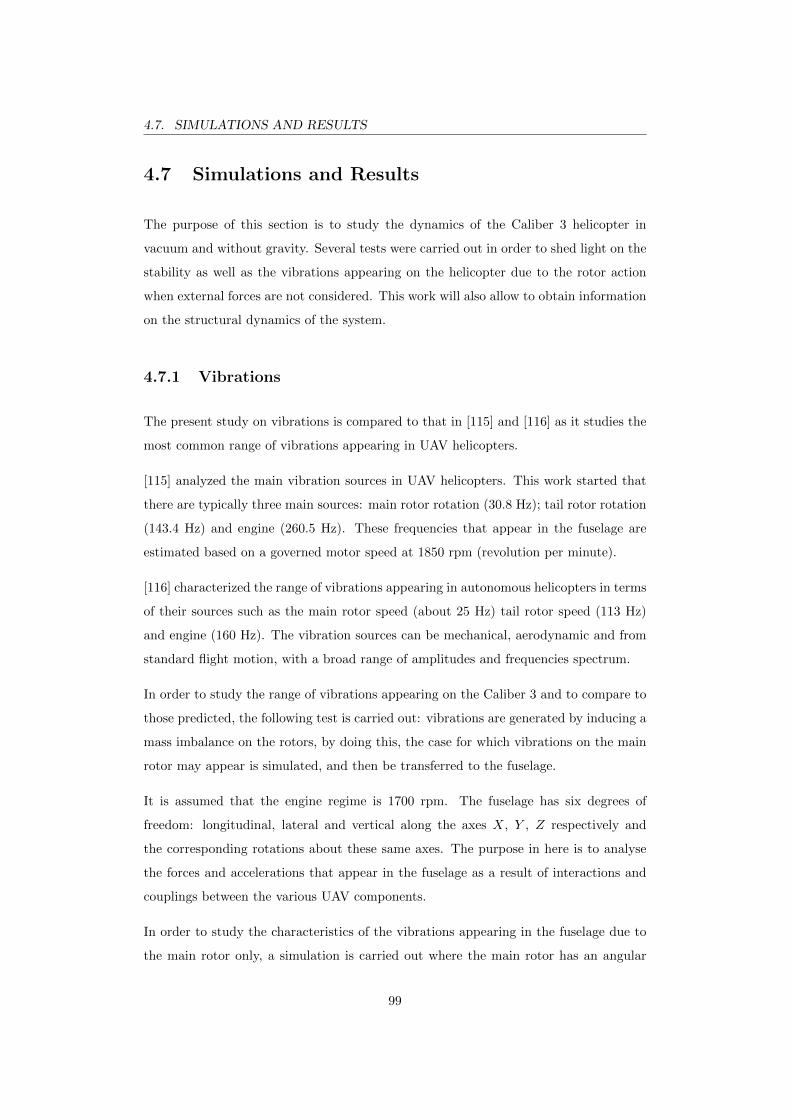
4.7. SIMULATIONS AND RESULTS
4.7 Simulations and Results
The purpose of this section is to study the dynamics of the Caliber 3 helicopter in
vacuum and without gravity. Several tests were carried out in order to shed light on the
stability as well as the vibrations appearing on the helicopter due to the rotor action
when external forces are not considered. This work will also allow to obtain information
on the structural dynamics of the system.
4.7.1 Vibrations
The present study on vibrations is compared to that in [115] and [116] as it studies the
most common range of vibrations appearing in UAV helicopters.
[115] analyzed the main vibration sources in UAV helicopters. This work started that
there are typically three main sources: main rotor rotation (30.8 Hz); tail rotor rotation
(143.4 Hz) and engine (260.5 Hz). These frequencies that appear in the fuselage are
estimated based on a governed motor speed at 1850 rpm (revolution per minute).
[116] characterized the range of vibrations appearing in autonomous helicopters in terms
of their sources such as the main rotor speed (about 25 Hz) tail rotor speed (113 Hz)
and engine (160 Hz). The vibration sources can be mechanical, aerodynamic and from
standard flight motion, with a broad range of amplitudes and frequencies spectrum.
In order to study the range of vibrations appearing on the Caliber 3 and to compare to
those predicted, the following test is carried out: vibrations are generated by inducing a
mass imbalance on the rotors, by doing this, the case for which vibrations on the main
rotor may appear is simulated, and then be transferred to the fuselage.
It is assumed that the engine regime is 1700 rpm. The fuselage has six degrees of
freedom: longitudinal, lateral and vertical along the axes X, Y , Z respectively and
the corresponding rotations about these same axes. The purpose in here is to analyse
the forces and accelerations that appear in the fuselage as a result of interactions and
couplings between the various UAV components.
In order to study the characteristics of the vibrations appearing in the fuselage due to
the main rotor only, a simulation is carried out where the main rotor has an angular
99
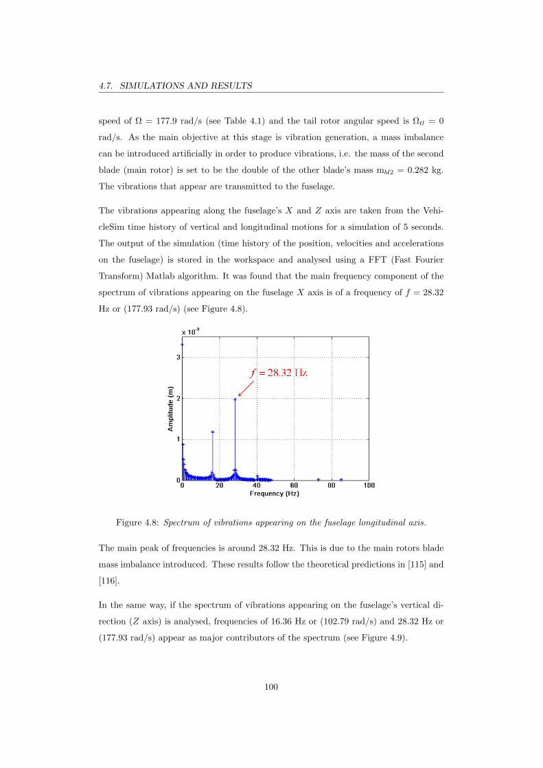
4.7. SIMULATIONS AND RESULTS
speed of Ω = 177.9 rad/s (see Table 4.1) and the tail rotor angular speed is Ωtl = 0
rad/s. As the main objective at this stage is vibration generation, a mass imbalance
can be introduced artificially in order to produce vibrations, i.e. the mass of the second
blade (main rotor) is set to be the double of the other blade’s mass mbl2 = 0.282 kg.
The vibrations that appear are transmitted to the fuselage.
The vibrations appearing along the fuselage’s X and Z axis are taken from the Vehi-
cleSim time history of vertical and longitudinal motions for a simulation of 5 seconds.
The output of the simulation (time history of the position, velocities and accelerations
on the fuselage) is stored in the workspace and analysed using a FFT (Fast Fourier
Transform) Matlab algorithm. It was found that the main frequency component of the
spectrum of vibrations appearing on the fuselage X axis is of a frequency of f = 28.32
Hz or (177.93 rad/s) (see Figure 4.8).
Figure 4.8: Spectrum of vibrations appearing on the fuselage longitudinal axis.
The main peak of frequencies is around 28.32 Hz. This is due to the main rotors blade
mass imbalance introduced. These results follow the theoretical predictions in [115] and
[116].
In the same way, if the spectrum of vibrations appearing on the fuselage’s vertical di-
rection (Z axis) is analysed, frequencies of 16.36 Hz or (102.79 rad/s) and 28.32 Hz or
(177.93 rad/s) appear as major contributors of the spectrum (see Figure 4.9).
100
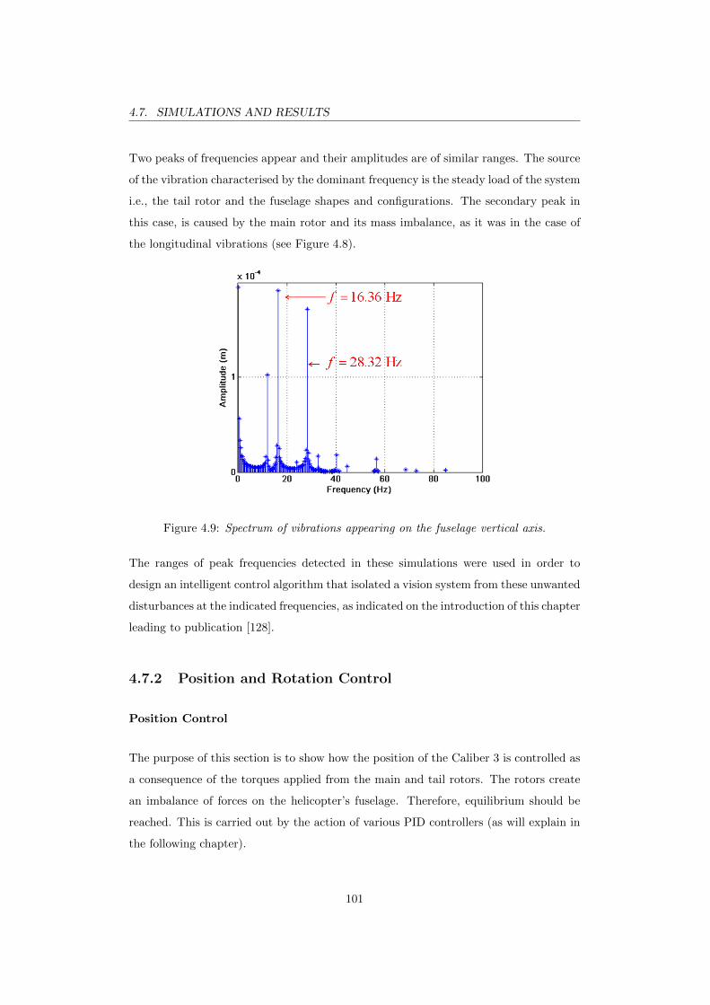
4.7. SIMULATIONS AND RESULTS
Two peaks of frequencies appear and their amplitudes are of similar ranges. The source
of the vibration characterised by the dominant frequency is the steady load of the system
i.e., the tail rotor and the fuselage shapes and configurations. The secondary peak in
this case, is caused by the main rotor and its mass imbalance, as it was in the case of
the longitudinal vibrations (see Figure 4.8).
Figure 4.9: Spectrum of vibrations appearing on the fuselage vertical axis.
The ranges of peak frequencies detected in these simulations were used in order to
design an intelligent control algorithm that isolated a vision system from these unwanted
disturbances at the indicated frequencies, as indicated on the introduction of this chapter
leading to publication [128].
4.7.2 Position and Rotation Control
Position Control
The purpose of this section is to show how the position of the Caliber 3 is controlled as
a consequence of the torques applied from the main and tail rotors. The rotors create
an imbalance of forces on the helicopter’s fuselage. Therefore, equilibrium should be
reached. This is carried out by the action of various PID controllers (as will explain in
the following chapter).
101
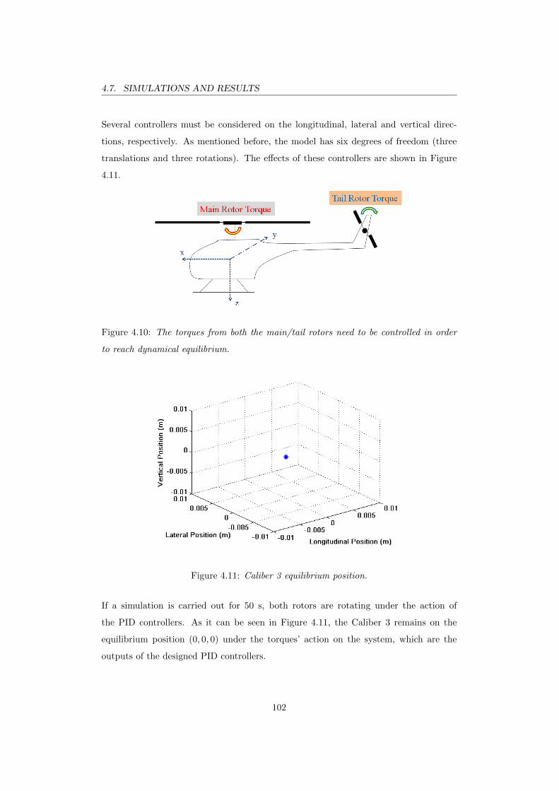
4.7. SIMULATIONS AND RESULTS
Several controllers must be considered on the longitudinal, lateral and vertical direc-
tions, respectively. As mentioned before, the model has six degrees of freedom (three
translations and three rotations). The effects of these controllers are shown in Figure
4.11.
Figure 4.10: The torques from both the main/tail rotors need to be controlled in order
to reach dynamical equilibrium.
Figure 4.11: Caliber 3 equilibrium position.
If a simulation is carried out for 50 s, both rotors are rotating under the action of
the PID controllers. As it can be seen in Figure 4.11, the Caliber 3 remains on the
equilibrium position (0, 0, 0) under the torques’ action on the system, which are the
outputs of the designed PID controllers.
102

4.8. CHAPTER SUMMARY
Rotation Control
In this section, three controllers were introduced on the roll, pitch and yaw, respectively,
in order to achieve rotational control of the helicopter. These will be presented in
Chapter 5 and details of their implementation will be provided. The action of these
controller is shown in Figure 4.12.
Figure 4.12: Caliber 3 equilibrium in rotation.
The equilibrium in rotation around the point (0, 0, 0) for the case of the Caliber 3
is clearly achieved as a result of the PID controllers being implemented in the three
rotational degrees of freedom.
4.8 Chapter Summary
This chapter contains the modelling details for a Caliber 3 (UAV) by using the Vehi-
cleSim. The model has been developed without the influence of any external force i.e.,
the system can be considered to be in vacuum and no aerodynamic loads were taken
into account. The main contribution of this chapter with respect to the following one
is that now the swashplate is implemented as a new body and the elevators are care-
fully described in order to show their behaviour on the system. Clearly, this is a more
complex model than the one shown in the following chapter.
103
4.8. CHAPTER SUMMARY
This work was carried out in collaboration with La Laguna University (Spain), during
a four months Erasmus research visit. The main task was to measure the physical
parameters such as fuselage weight, blade lengths, etc. The helicopter configuration was
as well analyzed in order to implement it in VehicleSim as a multibody system. After
that, some additional parameters were obtained by using Autodesk Inventor, however
the results from this software were not of enough accuracy for the VehicleSim parameters
requirement. For example, the centre of mass was not generated by Inventor. On the
contrary, centres of gravity were provided. Nevertheless, the obtained data were enough
to build up an initial Caliber 3 model in VehicleSim.
A physical description of the model was provided, the bodies, their degrees of freedom as
well as their linkages were identified. As it has been shown, the fuselage, the swashplate,
the main rotor and tail rotor have been modelled by using a parent-child relation in
VehicleSim. In addition to this, the connections between the several bodies have been
established and the degrees of freedom for each body have been included.
The main rotor has been described as a body composed of several hinges as well as
several degrees of freedom, these being the feather, lag and flap. The blades were added
as bodies with mass and inertial properties. Two elevators are also modelled on the
main rotor with mass and inertial properties. The swashplate was defined as a body
on the fuselage, being the parent of the main rotor; its action on the blades has been
included by using PID controllers. The elevator feather cyclic angle was designed and
modelled, showing the connection to the cyclic blade feather. The delta three angle and
its effects on the tail rotor have been modelled as well.
In addition to all these, this Caliber 3 model has been used to analyze the vibrations
appearing on the fuselage, as a consequence of mass imbalance on the main rotor. They
were used by the La Laguna University to develop robust control methodology for an
onboard vision system. The conditions to generate these vibrations were imposed by
them in order to get the vibrations with the correct characteristics to achieve their
control. The vibrations were provided in two axes because they requested only this
information. On the other hand, the vibrations obtained agreed with the experimen-
tal values proposed by various authors [115], [116], validating in the case the provided
model.
104
4.8. CHAPTER SUMMARY
Once the vibrations were generated, two torques were implemented in both rotors in
order to simulate the engine action. Whereas, this action produces that the system loses
the initial equilibrium around the point (0, 0, 0). Therefore, various PID controllers were
implemented and included in the model so that the initial equilibrium could be restored.
105

Chapter 5
Sikorsky Configuration
Dynamic Model
5.1 Introduction
The aim of this chapter is to present the modelling techniques developed to build the
VehicleSim code for a helicopter in Sikorsky configuration. The multibody structure and
the main modelling commands are presented in here. First of all, a general overview
of the helicopter model is given. This is followed by programming details and a de-
scription of the multibody model program in VehicleSim. The procedure is focused on
the fuselage, the main and tail rotors. The engine and the swashplate models are not
presented, but their actions are modelled and introduced in the program.
Helicopters are complex systems, composed by several bodies as well as several degrees
of freedoms, motions are allowed in three dimensions. The modelling of helicopter
dynamics is necessary in order to study the interactions between the different parts of
the helicopter and the instabilities on the system under various flight conditions.
There exits several studies carried out in this field but, the majority of existing models
have been built under linearised conditions [5], [42]. There are also some nonlinear works
on helicopter dynamics but mainly these are for reduced order models [44]. Therefore,
the modelling of the rotorcraft system by considering the nonlinear dynamics is an
106
5.1. INTRODUCTION
interesting and much needed task. A full model of a helicopter is developed by using
VehicleSim in order to capture the nonlinear behaviour of the system. This allows to
develop a comprehensive understanding of the interaction between the several parts
of the helicopter and their dynamics, whilst the linear analysis does not explain these
behaviours completely.
A helicopter can be defined as an aircraft that uses rotating wings to provide lift,
propulsion and control. It is made up as the combination of several subsystems such
as main rotor, fuselage, tail rotor and engine. In this chapter, the model under study
is known as Sikorsky configuration, it consists of one main rotor, fuselage and one tail
rotor mounted in perpendicular to the main rotor. The main rotor subsystem model in
here is based on a previous work [124]. It was built by using Autosim software (previous
version of VehicleSim).
The fuselage is the rotorcraft’s main body section that holds crew and passengers or
cargo. Its degrees of freedom are the lateral and longitudinal translation in the hor-
izontal plane X − Y axis, vertical translation in the Z axis and rotation about these
same axes corresponding to yaw, pitch and roll. The rotors of a helicopter, due to
its rotating nature, are prone to introducing vibrations on the fuselage that may af-
fect the aircraft’s performance, the passengers’ comfort and the accuracy of on board
measurement devices, for example, vision systems.
The role of the main rotor is to support the aircraft’s weight, as it generates the lift force.
It allows to keep the helicopter suspended in the air and provides the control that allows
to follow a prescribed trajectory in the various spatial directions by changing altitude
and executing turns. It transfers prevailingly aerodynamic forces and moments from
the rotating blades to the non-rotating frame (fuselage); a conventional rotor consists
of two or more identical equally spaced blades attached to a central hub. The blades
are kept in uniform rotational motion (rotational speed Ω), by a shaft torque from the
engine.
A common design solution adopted in the development of the helicopter is to use hinges
at the blades roots that allow blade free motion and in the plane of the disc, see Figure
5.1.
107
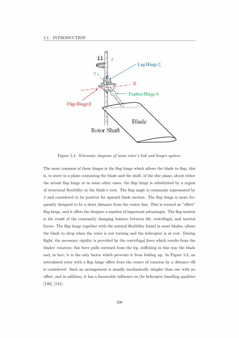
5.1. INTRODUCTION
Figure 5.1: Schematic diagram of main rotor’s hub and hinges system.
The most common of these hinges is the flap hinge which allows the blade to flap, this
is, to move in a plane containing the blade and the shaft, of the disc plane, about either
the actual flap hinge or in some other cases, the flap hinge is substituted by a region
of structural flexibility at the blade’s root. The flap angle is commonly represented by
β and considered to be positive for upward blade motion. The flap hinge is more fre-
quently designed to be a short distance from the centre line. This is termed as ”offset”
flap hinge, and it offers the designer a number of important advantages. The flap motion
is the result of the constantly changing balance between lift, centrifugal, and inertial
forces. The flap hinge together with the natural flexibility found in most blades, allows
the blade to drop when the rotor is not turning and the helicopter is at rest. During
flight, the necessary rigidity is provided by the centrifugal force which results from the
blades’ rotation; this force pulls outward from the tip, stiffening in this way the blade
and, in fact, it is the only factor which prevents it from folding up. In Figure 5.2, an
articulated rotor with a flap hinge offset from the centre of rotation by a distance eR
is considered. Such an arrangement is usually mechanically simpler than one with no
offset, and in addition, it has a favourable influence on the helicopter handling qualities
[140], [141].
108
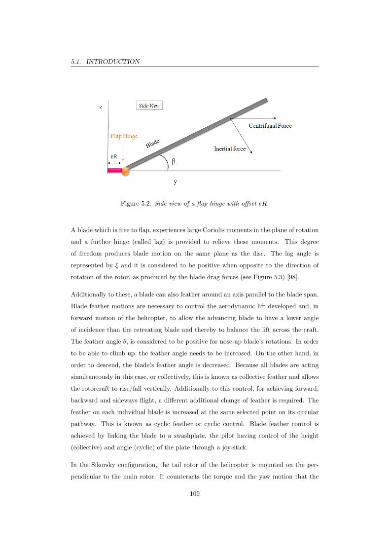
5.1. INTRODUCTION
Figure 5.2: Side view of a flap hinge with offset eR.
A blade which is free to flap, experiences large Coriolis moments in the plane of rotation
and a further hinge (called lag) is provided to relieve these moments. This degree
of freedom produces blade motion on the same plane as the disc. The lag angle is
represented by ξ and it is considered to be positive when opposite to the direction of
rotation of the rotor, as produced by the blade drag forces (see Figure 5.3) [98].
Additionally to these, a blade can also feather around an axis parallel to the blade span.
Blade feather motions are necessary to control the aerodynamic lift developed and, in
forward motion of the helicopter, to allow the advancing blade to have a lower angle
of incidence than the retreating blade and thereby to balance the lift across the craft.
The feather angle θ, is considered to be positive for nose-up blade’s rotations. In order
to be able to climb up, the feather angle needs to be increased. On the other hand, in
order to descend, the blade’s feather angle is decreased. Because all blades are acting
simultaneously in this case, or collectively, this is known as collective feather and allows
the rotorcraft to rise/fall vertically. Additionally to this control, for achieving forward,
backward and sideways flight, a different additional change of feather is required. The
feather on each individual blade is increased at the same selected point on its circular
pathway. This is known as cyclic feather or cyclic control. Blade feather control is
achieved by linking the blade to a swashplate, the pilot having control of the height
(collective) and angle (cyclic) of the plate through a joy-stick.
In the Sikorsky configuration, the tail rotor of the helicopter is mounted on the per-
pendicular to the main rotor. It counteracts the torque and the yaw motion that the
109
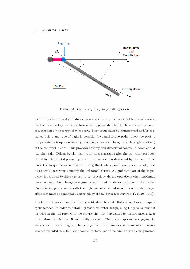
5.1. INTRODUCTION
Figure 5.3: Top view of a lag hinge with offset eR.
main rotor disc naturally produces. In accordance to Newton’s third law of action and
reaction, the fuselage tends to rotate on the opposite direction to the main rotor’s blades
as a reaction of the torque that appears. This torque must be counteracted and/or con-
trolled before any type of flight is possible. Two anti-torque pedals allow the pilot to
compensate for torque variance by providing a means of changing pitch (angle of attack)
of the tail rotor blades. This provides heading and directional control in hover and at
low airspeeds. Driven by the main rotor at a constant ratio, the tail rotor produces
thrust in a horizontal plane opposite to torque reaction developed by the main rotor.
Since the torque magnitude varies during flight when power changes are made, it is
necessary to accordingly modify the tail rotor’s thrust. A significant part of the engine
power is required to drive the tail rotor, especially during operations when maximum
power is used. Any change in engine power output produces a change in the torque.
Furthermore, power varies with the flight manoeuvre and results in a variable torque
effect that must be continually corrected, by the tail rotor (see Figure 5.4), ([140]- [143]).
The tail rotor has no need for the disc attitude to be controlled and so does not require
cyclic feather. In order to obtain lightest a tail rotor design, a lag hinge is usually not
included in the tail rotor with the proviso that any flap caused by disturbances is kept
to an absolute minimum if not totally avoided. The blade flap can be triggered by
the effects of forward flight or by aerodynamic disturbances and means of minimising
this are included in a tail rotor control system, known as ”delta-three” configuration.
110

5.1. INTRODUCTION
Figure 5.4: Tail rotor counteracting the torque induced by the main rotor rotation.
In addition to this, this coupling is designed to reduce transient flap angles and blade
stresses [142], [144]. The feather-flap coupling is a kinematic feedback of the flap angular
displacement to the blade feather motion that can be algebraically described as:
∆θ = −kβ (5.1)
where θ is the feather angle and k is the feather-flap coupling coefficient. This acts
as an aerodynamic spring for the flap mode because the lower feather means less lift.
The feather-flap coupling plays an important role in flight stability and the handling
qualities of the vehicle as well as aeroelastic blade’s stability. The simplest approach is
to skew the flap hinge by an angle (”delta-three”) so that it is not longer perpendicular
to the blade radial axis. Then a rotation about the hinge with a flap angle β must
also produce a feather change of −βtanδ3. The feedback gain for this arrangement is
therefore k = tanδ3. Feather-flap coupling is defined in terms of the delta three angle
(see Figure 5.5) [140].
111
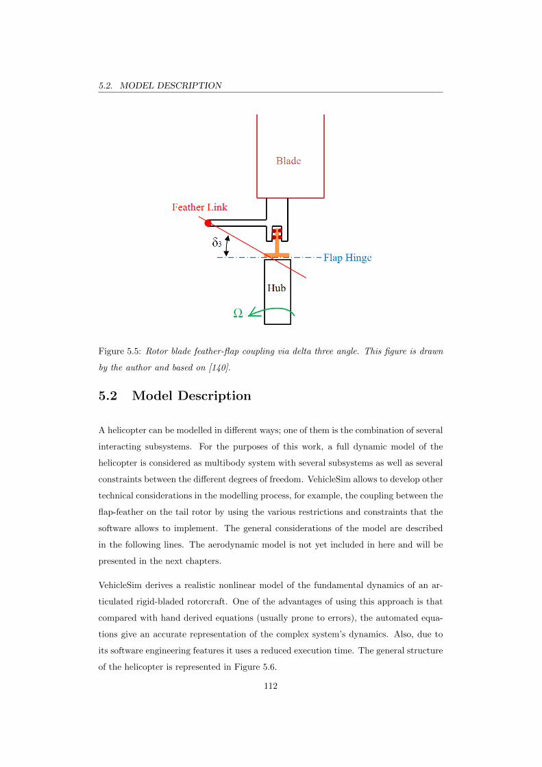
5.2. MODEL DESCRIPTION
Figure 5.5: Rotor blade feather-flap coupling via delta three angle. This figure is drawn
by the author and based on [140].
5.2 Model Description
A helicopter can be modelled in different ways; one of them is the combination of several
interacting subsystems. For the purposes of this work, a full dynamic model of the
helicopter is considered as multibody system with several subsystems as well as several
constraints between the different degrees of freedom. VehicleSim allows to develop other
technical considerations in the modelling process, for example, the coupling between the
flap-feather on the tail rotor by using the various restrictions and constraints that the
software allows to implement. The general considerations of the model are described
in the following lines. The aerodynamic model is not yet included in here and will be
presented in the next chapters.
VehicleSim derives a realistic nonlinear model of the fundamental dynamics of an ar-
ticulated rigid-bladed rotorcraft. One of the advantages of using this approach is that
compared with hand derived equations (usually prone to errors), the automated equa-
tions give an accurate representation of the complex system’s dynamics. Also, due to
its software engineering features it uses a reduced execution time. The general structure
of the helicopter is represented in Figure 5.6.
112
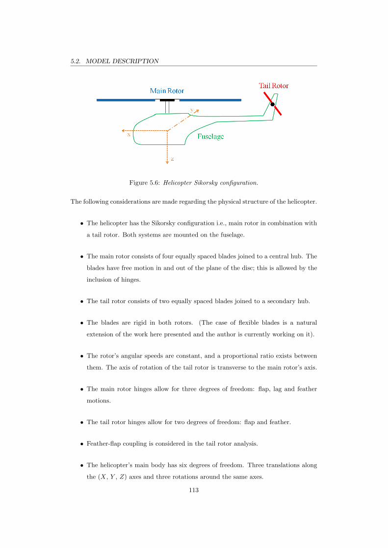
5.2. MODEL DESCRIPTION
Figure 5.6: Helicopter Sikorsky configuration.
The following considerations are made regarding the physical structure of the helicopter.
• The helicopter has the Sikorsky configuration i.e., main rotor in combination with
a tail rotor. Both systems are mounted on the fuselage.
• The main rotor consists of four equally spaced blades joined to a central hub. The
blades have free motion in and out of the plane of the disc; this is allowed by the
inclusion of hinges.
• The tail rotor consists of two equally spaced blades joined to a secondary hub.
• The blades are rigid in both rotors. (The case of flexible blades is a natural
extension of the work here presented and the author is currently working on it).
• The rotor’s angular speeds are constant, and a proportional ratio exists between
them. The axis of rotation of the tail rotor is transverse to the main rotor’s axis.
• The main rotor hinges allow for three degrees of freedom: flap, lag and feather
motions.
• The tail rotor hinges allow for two degrees of freedom: flap and feather.
• Feather-flap coupling is considered in the tail rotor analysis.
• The helicopter’s main body has six degrees of freedom. Three translations along
the (X, Y , Z) axes and three rotations around the same axes.
113
5.3. DYNAMIC MODEL
5.3 Dynamic Model
VehicleSim (Version 1.0, August 2008) Lisp is used to develop the multibody system
code that represents the helicopter system as described in section 5.2 (see Figure 5.6).
The multibody system is subdivided into its constituent bodies for the purpose of writing
the VehicleSim code. The bodies are arranged as a parent-child relationship as shown in
Figure 5.7. In VehicleSim, each reference frame has a rectangular 3D coordinate system
that associates a unique ordered trio of numbers to each point fixed in that reference
frame. n is the inertial reference frame. As new bodies are added to the system, having
freedoms relative to n, local origins and axes are defined. All VehicleSim coordinate
systems are right-handed Cartesian systems defined, by (i) a reference frame in which
the coordinate system is fixed, (ii) an origin point, and (iii) three mutually orthogonal
directions that define the axes. By ”right handed”, it means that if two of the directions
are X and Y , then the third direction z = x×y. The body-fixed points coincide with the
corresponding global points, fixed in n, when the system is on its nominal configuration.
Most points are fixed in bodies but a point may be defined as mobile with its location
in a body determined from its specified coordinates. This is useful for describing time
varying points of contact between one body and another one. The code starts with
an inertial reference frame n, with fixed origin, n0, and fixed directions [nx],[ny] and
[nz] already defined [134]. The first body included in the code is the fuselage, it is
implemented as the child of the nominal reference frame. The fuselage is located at the
origin of the inertial coordinates system and it is the parent of both the main and tail
rotors. The main rotor rotates around its vertical axis, Z axis. The main rotor is the
parent of the flap hinges that rotates around the corresponding X axis, each lag hinge
is the child of the corresponding flap hinge. The lag hinges rotate around the Z axis.
The feather hinges are the child of the lag hinges. Each feather hinge rotates around the
Y axis. Finally, a blade is added to the program structure as the child of each feather
hinge. The tail rotor is built up following this same parent-child structure.
(reset)
(si)
(add-gravity)
(setf *linear* t) ; or (nil if nonlinear simulation is needed)
114
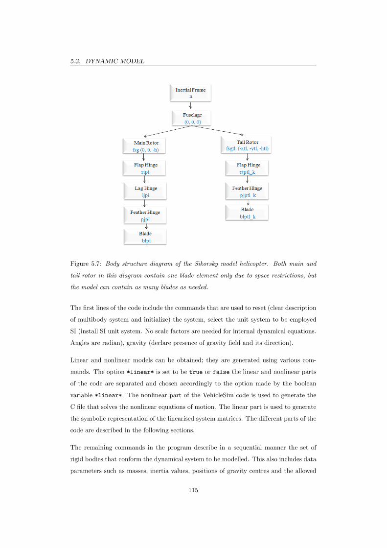
5.3. DYNAMIC MODEL
Figure 5.7: Body structure diagram of the Sikorsky model helicopter. Both main and
tail rotor in this diagram contain one blade element only due to space restrictions, but
the model can contain as many blades as needed.
The first lines of the code include the commands that are used to reset (clear description
of multibody system and initialize) the system, select the unit system to be employed
SI (install SI unit system. No scale factors are needed for internal dynamical equations.
Angles are radian), gravity (declare presence of gravity field and its direction).
Linear and nonlinear models can be obtained; they are generated using various com-
mands. The option *linear* is set to be true or false the linear and nonlinear parts
of the code are separated and chosen accordingly to the option made by the boolean
variable *linear*. The nonlinear part of the VehicleSim code is used to generate the
C file that solves the nonlinear equations of motion. The linear part is used to generate
the symbolic representation of the linearised system matrices. The different parts of the
code are described in the following sections.
The remaining commands in the program describe in a sequential manner the set of
rigid bodies that conform the dynamical system to be modelled. This also includes data
parameters such as masses, inertia values, positions of gravity centres and the allowed
115
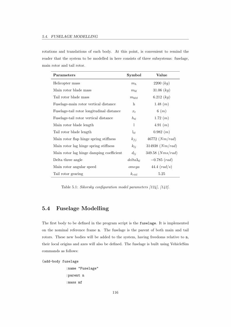
5.4. FUSELAGE MODELLING
rotations and translations of each body. At this point, is convenient to remind the
reader that the system to be modelled in here consists of three subsystems: fuselage,
main rotor and tail rotor.
Parameters Symbol Value
Helicopter mass mh 2200 (kg)
Main rotor blade mass mbl 31.06 (kg)
Tail rotor blade mass mbltl 6.212 (kg)
Fuselage-main rotor vertical distance h 1.48 (m)
Fuselage-tail rotor longitudinal distance xt 6 (m)
Fuselage-tail rotor vertical distance htl 1.72 (m)
Main rotor blade length l 4.91 (m)
Tail rotor blade length ltl 0.982 (m)
Main rotor flap hinge spring stiffness kfj 46772 (Nm/rad)
Main rotor lag hinge spring stiffness klj 314938 (Nm/rad)
Main rotor lag hinge damping coefficient dlj 349.58 (Nms/rad)
Delta three angle delta3tl −0.785 (rad)
Main rotor angular speed omega 44.4 (rad/s)
Tail rotor gearing krttl 5.25
Table 5.1: Sikorsky configuration model parameters [124], [142].
5.4 Fuselage Modelling
The first body to be defined in the program script is the fuselage. It is implemented
on the nominal reference frame n. The fuselage is the parent of both main and tail
rotors. These new bodies will be added to the system, having freedoms relative to n,
their local origins and axes will also be defined. The fuselage is built using VehicleSim
commands as follows:
(add-body fuselage
:name "Fuselage"
:parent n
:mass mf
116
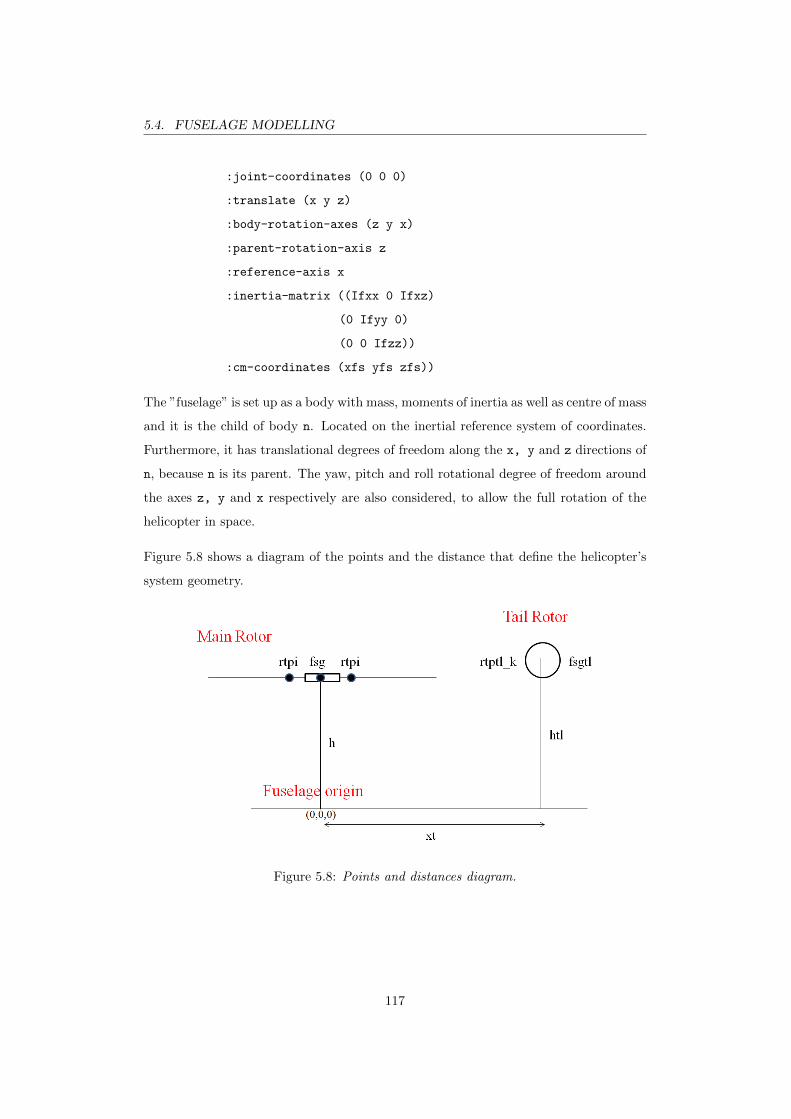
5.4. FUSELAGE MODELLING
:joint-coordinates (0 0 0)
:translate (x y z)
:body-rotation-axes (z y x)
:parent-rotation-axis z
:reference-axis x
:inertia-matrix ((Ifxx 0 Ifxz)
(0 Ifyy 0)
(0 0 Ifzz))
:cm-coordinates (xfs yfs zfs))
The ”fuselage” is set up as a body with mass, moments of inertia as well as centre of mass
and it is the child of body n. Located on the inertial reference system of coordinates.
Furthermore, it has translational degrees of freedom along the x, y and z directions of
n, because n is its parent. The yaw, pitch and roll rotational degree of freedom around
the axes z, y and x respectively are also considered, to allow the full rotation of the
helicopter in space.
Figure 5.8 shows a diagram of the points and the distance that define the helicopter’s
system geometry.
Figure 5.8: Points and distances diagram.
117

5.5. MAIN ROTOR MODELLING
5.5 Main Rotor Modelling
5.5.1 Bodies Definition
The main rotor is built on a similar parent-child structure. First, the main rotor is
implemented as a child of the fuselage, and it will be the parent of the corresponding
subsystems. The rotor is connected to the fuselage at the point fsg (see Figure 5.8)
which needs to be defined prior to the main rotor definition.
(add-point fsg :body fuselage :coordinates (0 0 -h))
The point fsg is located at a vertical distance -h from the origin of the inertial axes
system. Note that the negative sign of the vertical distance h, is due to VehicleSim sign
convention of considering the positive vertical direction to be downwards.
The main rotor is introduced into the model:
(add-body rt
:name "Rotor"
:parent fuselage
:mass 0
:joint-coordinates fsg
:body-rotation-axes z
:parent-rotation-axis z
:reference-axis x
:inertia-matrix(0 0 Irtz))
The ”rotor” is set up as a massless body. The rotational degree of freedom around
the axes Z is considered. The coordinates of the joint between the main rotor and
the fuselage is given by the command :joint-coordinates, (its numerical value was
previously defined by the point fsg). Finally, its moments of inertia are also provided.
The main rotor has four blades equally spaced, this can be generalized to any number
of blades that may be required. The relative position of each of the blades with respect
to the main rotor axes origin is important in order to define the joining points to which
the hinges will be attached. The separation angle between each of the blades on the
main rotor disc can defined as alphai, with i = (1, ..., j), being j the total number of
118
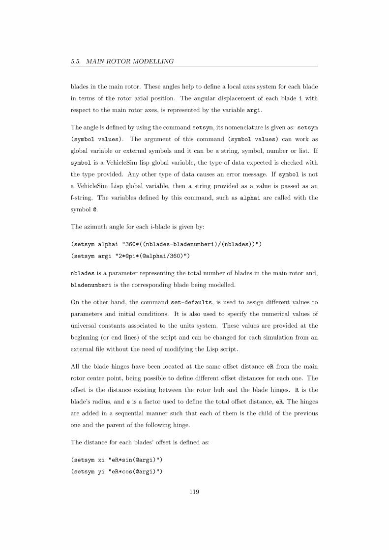
5.5. MAIN ROTOR MODELLING
blades in the main rotor. These angles help to define a local axes system for each blade
in terms of the rotor axial position. The angular displacement of each blade i with
respect to the main rotor axes, is represented by the variable argi.
The angle is defined by using the command setsym, its nomenclature is given as: setsym
(symbol values). The argument of this command (symbol values) can work as
global variable or external symbols and it can be a string, symbol, number or list. If
symbol is a VehicleSim lisp global variable, the type of data expected is checked with
the type provided. Any other type of data causes an error message. If symbol is not
a VehicleSim Lisp global variable, then a string provided as a value is passed as an
f-string. The variables defined by this command, such as alphai are called with the
symbol @.
The azimuth angle for each i-blade is given by:
(setsym alphai "360*((nblades-bladenumberi)/(nblades))")
(setsym argi "2*@pi*(@alphai/360)")
nblades is a parameter representing the total number of blades in the main rotor and,
bladenumberi is the corresponding blade being modelled.
On the other hand, the command set-defaults, is used to assign different values to
parameters and initial conditions. It is also used to specify the numerical values of
universal constants associated to the units system. These values are provided at the
beginning (or end lines) of the script and can be changed for each simulation from an
external file without the need of modifying the Lisp script.
All the blade hinges have been located at the same offset distance eR from the main
rotor centre point, being possible to define different offset distances for each one. The
offset is the distance existing between the rotor hub and the blade hinges. R is the
blade’s radius, and e is a factor used to define the total offset distance, eR. The hinges
are added in a sequential manner such that each of them is the child of the previous
one and the parent of the following hinge.
The distance for each blades’ offset is defined as:
(setsym xi "eR*sin(@argi)")
(setsym yi "eR*cos(@argi)")
119
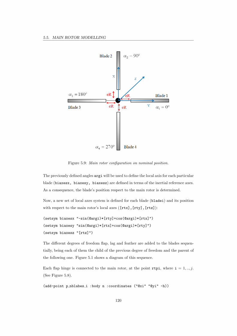
5.5. MAIN ROTOR MODELLING
Figure 5.9: Main rotor configuration on nominal position.
The previously defined angles argi will be used to define the local axis for each particular
blade (biaxesx, biaxesy, biaxesz) are defined in terms of the inertial reference axes.
As a consequence, the blade’s position respect to the main rotor is determined.
Now, a new set of local axes system is defined for each blade (bladei) and its position
with respect to the main rotor’s local axes ([rtx],[rty],[rtz]):
(setsym biaxesx "-sin(@argi)*[rty]+cos(@argi)*[rtx]")
(setsym biaxesy "sin(@argi)*[rtx]+cos(@argi)*[rty]")
(setsym biaxesz "[rtz]")
The different degrees of freedom flap, lag and feather are added to the blades sequen-
tially, being each of them the child of the previous degree of freedom and the parent of
the following one. Figure 5.1 shows a diagram of this sequence.
Each flap hinge is connected to the main rotor, at the point rtpi, where i = 1, .., j.
(See Figure 5.8).
(add-point p nblabes i :body n :coordinates ("@xi" "@yi" -h))
120
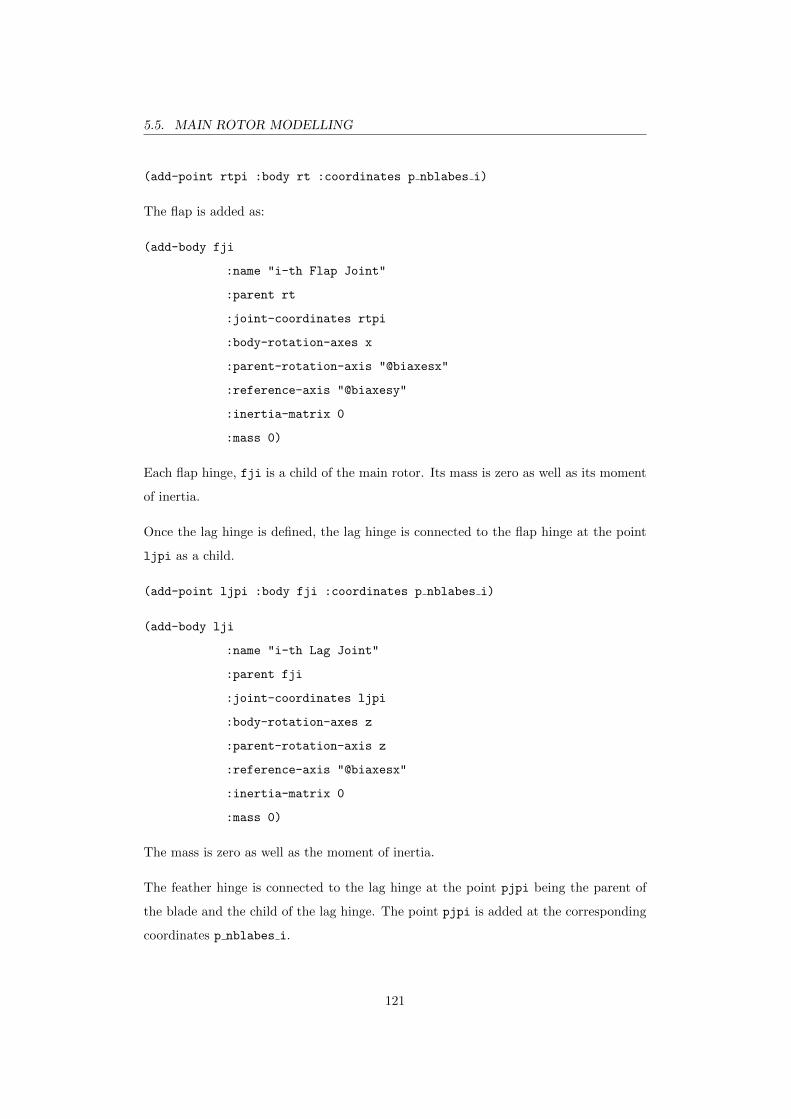
5.5. MAIN ROTOR MODELLING
(add-point rtpi :body rt :coordinates p nblabes i)
The flap is added as:
(add-body fji
:name "i-th Flap Joint"
:parent rt
:joint-coordinates rtpi
:body-rotation-axes x
:parent-rotation-axis "@biaxesx"
:reference-axis "@biaxesy"
:inertia-matrix 0
:mass 0)
Each flap hinge, fji is a child of the main rotor. Its mass is zero as well as its moment
of inertia.
Once the lag hinge is defined, the lag hinge is connected to the flap hinge at the point
ljpi as a child.
(add-point ljpi :body fji :coordinates p nblabes i)
(add-body lji
:name "i-th Lag Joint"
:parent fji
:joint-coordinates ljpi
:body-rotation-axes z
:parent-rotation-axis z
:reference-axis "@biaxesx"
:inertia-matrix 0
:mass 0)
The mass is zero as well as the moment of inertia.
The feather hinge is connected to the lag hinge at the point pjpi being the parent of
the blade and the child of the lag hinge. The point pjpi is added at the corresponding
coordinates p nblabes i.
121
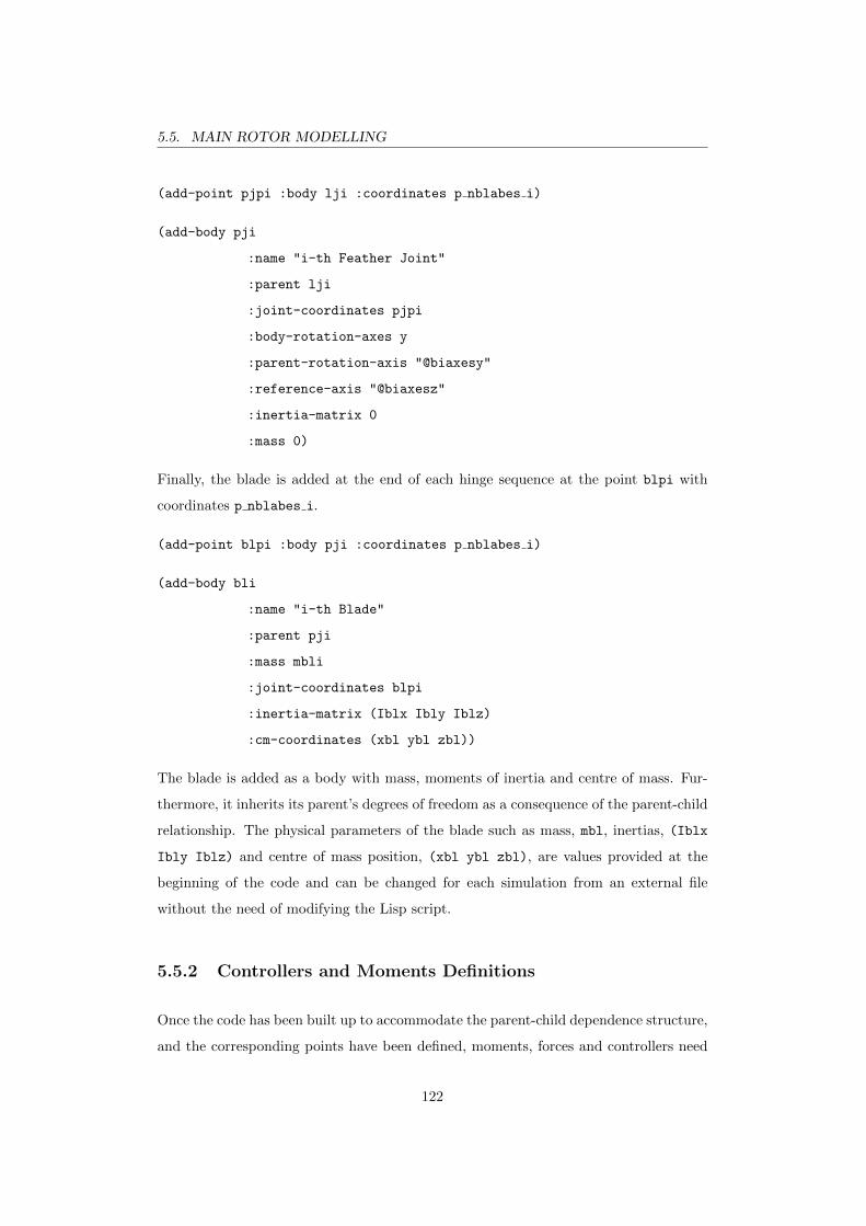
5.5. MAIN ROTOR MODELLING
(add-point pjpi :body lji :coordinates p nblabes i)
(add-body pji
:name "i-th Feather Joint"
:parent lji
:joint-coordinates pjpi
:body-rotation-axes y
:parent-rotation-axis "@biaxesy"
:reference-axis "@biaxesz"
:inertia-matrix 0
:mass 0)
Finally, the blade is added at the end of each hinge sequence at the point blpi with
coordinates p nblabes i.
(add-point blpi :body pji :coordinates p nblabes i)
(add-body bli
:name "i-th Blade"
:parent pji
:mass mbli
:joint-coordinates blpi
:inertia-matrix (Iblx Ibly Iblz)
:cm-coordinates (xbl ybl zbl))
The blade is added as a body with mass, moments of inertia and centre of mass. Fur-
thermore, it inherits its parent’s degrees of freedom as a consequence of the parent-child
relationship. The physical parameters of the blade such as mass, mbl, inertias, (Iblx
Ibly Iblz) and centre of mass position, (xbl ybl zbl), are values provided at the
beginning of the code and can be changed for each simulation from an external file
without the need of modifying the Lisp script.
5.5.2 Controllers and Moments Definitions
Once the code has been built up to accommodate the parent-child dependence structure,
and the corresponding points have been defined, moments, forces and controllers need
122
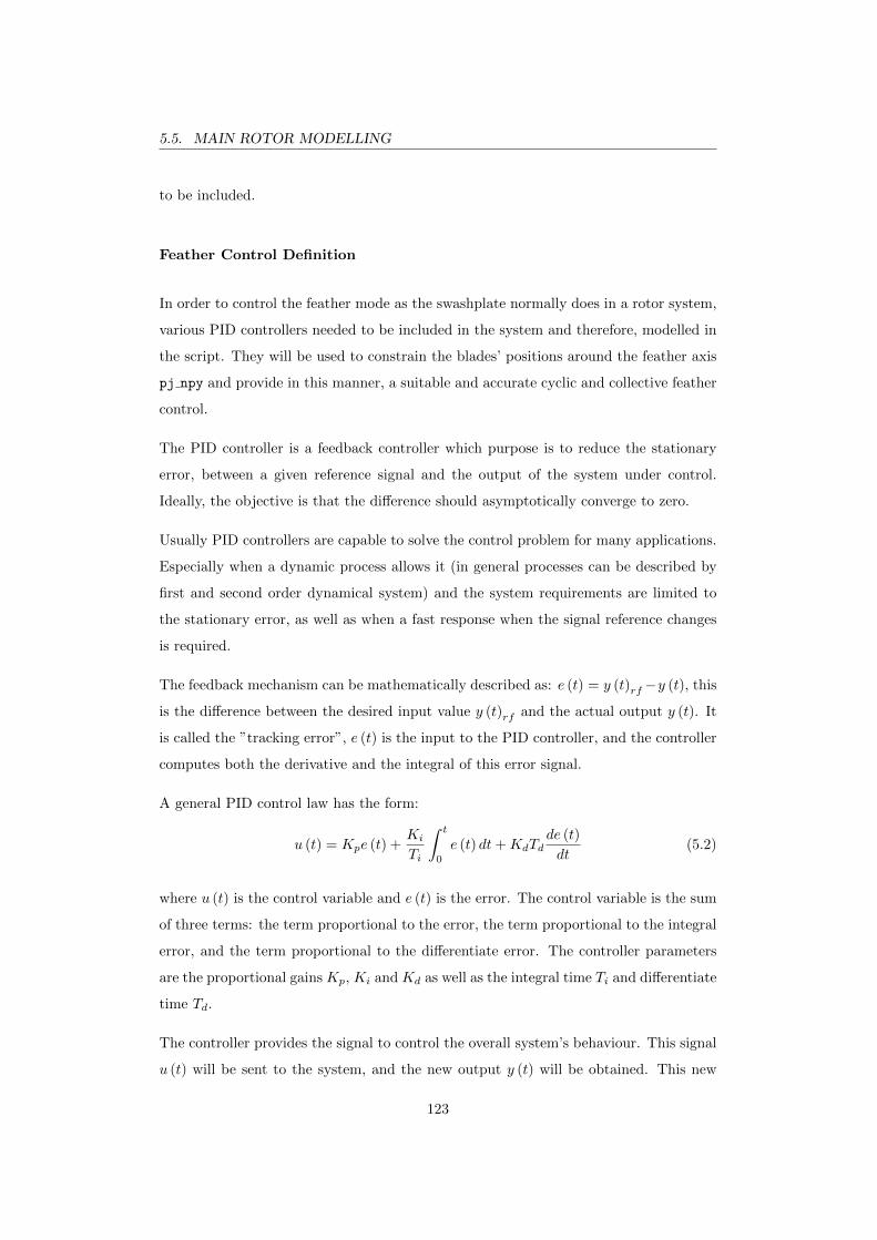
5.5. MAIN ROTOR MODELLING
to be included.
Feather Control Definition
In order to control the feather mode as the swashplate normally does in a rotor system,
various PID controllers needed to be included in the system and therefore, modelled in
the script. They will be used to constrain the blades’ positions around the feather axis
pj npy and provide in this manner, a suitable and accurate cyclic and collective feather
control.
The PID controller is a feedback controller which purpose is to reduce the stationary
error, between a given reference signal and the output of the system under control.
Ideally, the objective is that the difference should asymptotically converge to zero.
Usually PID controllers are capable to solve the control problem for many applications.
Especially when a dynamic process allows it (in general processes can be described by
first and second order dynamical system) and the system requirements are limited to
the stationary error, as well as when a fast response when the signal reference changes
is required.
The feedback mechanism can be mathematically described as: e (t) = y (t)rf−y (t), this
is the difference between the desired input value y (t)rf and the actual output y (t). It
is called the ”tracking error”, e (t) is the input to the PID controller, and the controller
computes both the derivative and the integral of this error signal.
A general PID control law has the form:
u (t) = Kpe (t) +Ki
Ti
∫ t
0
e (t) dt+KdTdde (t)
dt(5.2)
where u (t) is the control variable and e (t) is the error. The control variable is the sum
of three terms: the term proportional to the error, the term proportional to the integral
error, and the term proportional to the differentiate error. The controller parameters
are the proportional gains Kp, Ki and Kd as well as the integral time Ti and differentiate
time Td.
The controller provides the signal to control the overall system’s behaviour. This signal
u (t) will be sent to the system, and the new output y (t) will be obtained. This new
123
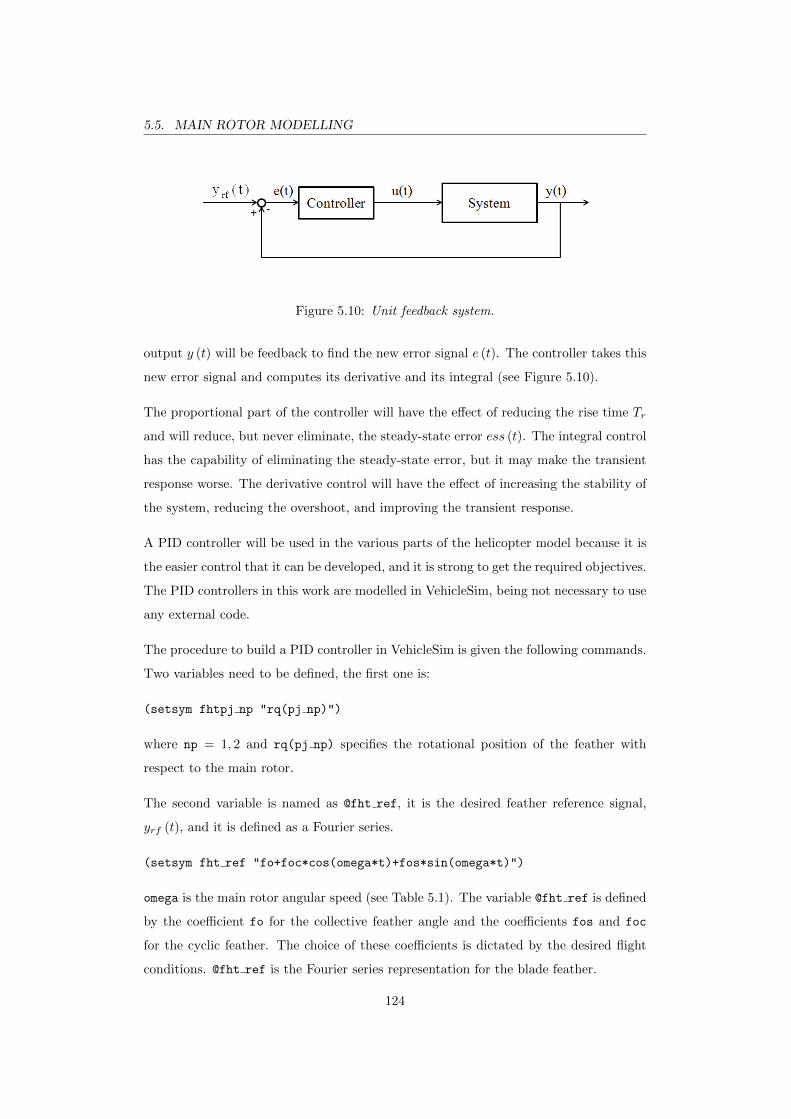
5.5. MAIN ROTOR MODELLING
Figure 5.10: Unit feedback system.
output y (t) will be feedback to find the new error signal e (t). The controller takes this
new error signal and computes its derivative and its integral (see Figure 5.10).
The proportional part of the controller will have the effect of reducing the rise time Tr
and will reduce, but never eliminate, the steady-state error ess (t). The integral control
has the capability of eliminating the steady-state error, but it may make the transient
response worse. The derivative control will have the effect of increasing the stability of
the system, reducing the overshoot, and improving the transient response.
A PID controller will be used in the various parts of the helicopter model because it is
the easier control that it can be developed, and it is strong to get the required objectives.
The PID controllers in this work are modelled in VehicleSim, being not necessary to use
any external code.
The procedure to build a PID controller in VehicleSim is given the following commands.
Two variables need to be defined, the first one is:
(setsym fhtpj np "rq(pj np)")
where np = 1, 2 and rq(pj np) specifies the rotational position of the feather with
respect to the main rotor.
The second variable is named as @fht ref, it is the desired feather reference signal,
yrf (t), and it is defined as a Fourier series.
(setsym fht ref "fo+foc*cos(omega*t)+fos*sin(omega*t)")
omega is the main rotor angular speed (see Table 5.1). The variable @fht ref is defined
by the coefficient fo for the collective feather angle and the coefficients fos and foc
for the cyclic feather. The choice of these coefficients is dictated by the desired flight
conditions. @fht ref is the Fourier series representation for the blade feather.
124
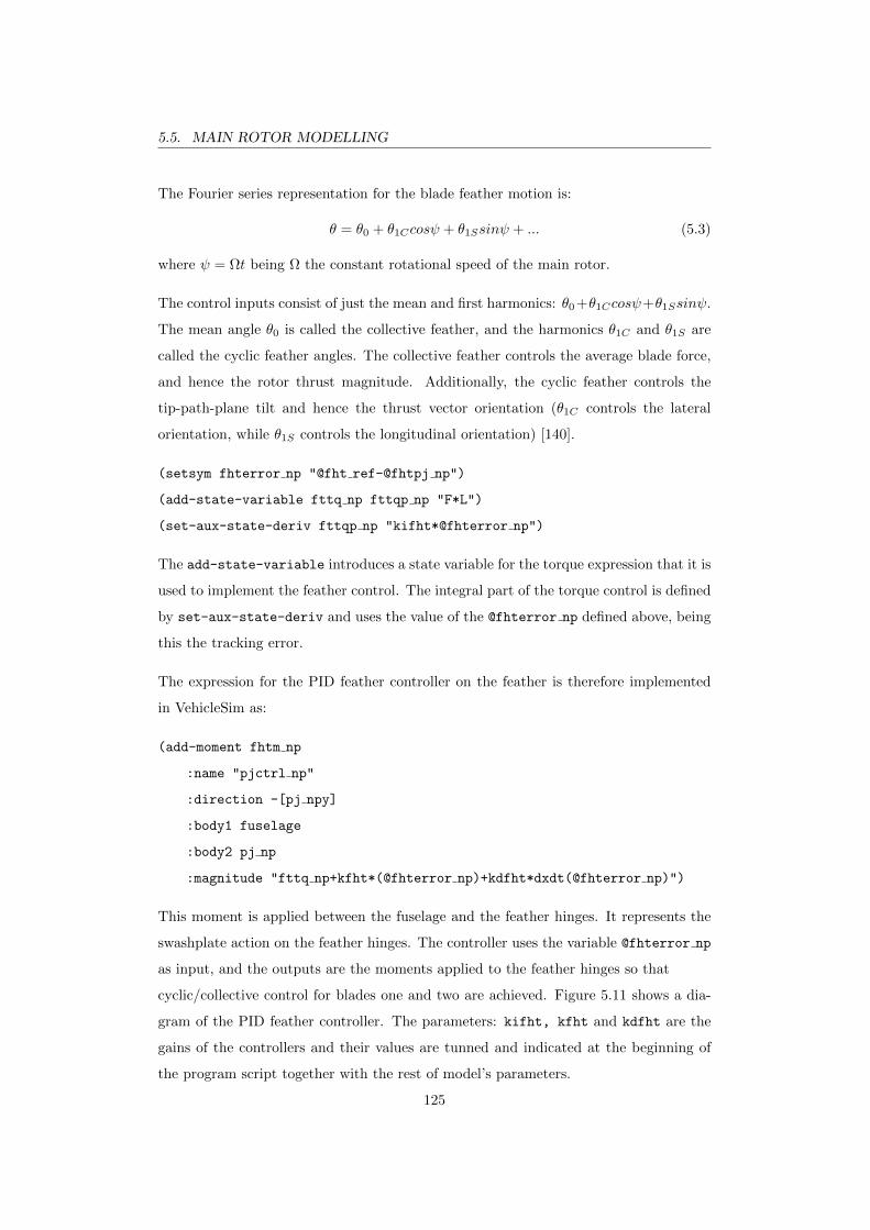
5.5. MAIN ROTOR MODELLING
The Fourier series representation for the blade feather motion is:
θ = θ0 + θ1Ccosψ + θ1Ssinψ + ... (5.3)
where ψ = Ωt being Ω the constant rotational speed of the main rotor.
The control inputs consist of just the mean and first harmonics: θ0 +θ1Ccosψ+θ1Ssinψ.
The mean angle θ0 is called the collective feather, and the harmonics θ1C and θ1S are
called the cyclic feather angles. The collective feather controls the average blade force,
and hence the rotor thrust magnitude. Additionally, the cyclic feather controls the
tip-path-plane tilt and hence the thrust vector orientation (θ1C controls the lateral
orientation, while θ1S controls the longitudinal orientation) [140].
(setsym fhterror np "@fht ref-@fhtpj np")
(add-state-variable fttq np fttqp np "F*L")
(set-aux-state-deriv fttqp np "kifht*@fhterror np")
The add-state-variable introduces a state variable for the torque expression that it is
used to implement the feather control. The integral part of the torque control is defined
by set-aux-state-deriv and uses the value of the @fhterror np defined above, being
this the tracking error.
The expression for the PID feather controller on the feather is therefore implemented
in VehicleSim as:
(add-moment fhtm np
:name "pjctrl np"
:direction -[pj npy]
:body1 fuselage
:body2 pj np
:magnitude "fttq np+kfht*(@fhterror np)+kdfht*dxdt(@fhterror np)")
This moment is applied between the fuselage and the feather hinges. It represents the
swashplate action on the feather hinges. The controller uses the variable @fhterror np
as input, and the outputs are the moments applied to the feather hinges so that
cyclic/collective control for blades one and two are achieved. Figure 5.11 shows a dia-
gram of the PID feather controller. The parameters: kifht, kfht and kdfht are the
gains of the controllers and their values are tunned and indicated at the beginning of
the program script together with the rest of model’s parameters.
125
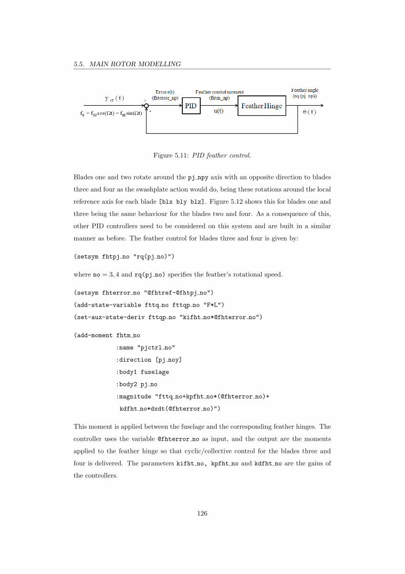
5.5. MAIN ROTOR MODELLING
Figure 5.11: PID feather control.
Blades one and two rotate around the pj npy axis with an opposite direction to blades
three and four as the swashplate action would do, being these rotations around the local
reference axis for each blade [blx bly blz]. Figure 5.12 shows this for blades one and
three being the same behaviour for the blades two and four. As a consequence of this,
other PID controllers need to be considered on this system and are built in a similar
manner as before. The feather control for blades three and four is given by:
(setsym fhtpj no "rq(pj no)")
where no = 3, 4 and rq(pj no) specifies the feather’s rotational speed.
(setsym fhterror no "@fhtref-@fhtpj no")
(add-state-variable fttq no fttqp no "F*L")
(set-aux-state-deriv fttqp no "kifht no*@fhterror no")
(add-moment fhtm no
:name "pjctrl no"
:direction [pj noy]
:body1 fuselage
:body2 pj no
:magnitude "fttq no+kpfht no*(@fhterror no)+
kdfht no*dxdt(@fhterror no)")
This moment is applied between the fuselage and the corresponding feather hinges. The
controller uses the variable @fhterror no as input, and the output are the moments
applied to the feather hinge so that cyclic/collective control for the blades three and
four is delivered. The parameters kifht no, kpfht no and kdfht no are the gains of
the controllers.
126
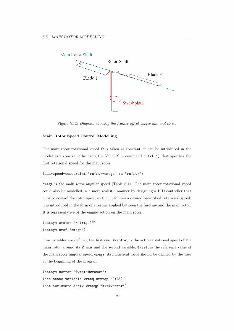
5.5. MAIN ROTOR MODELLING
Figure 5.12: Diagram showing the feather effect blades one and three.
Main Rotor Speed Control Modelling
The main rotor rotational speed Ω is taken as constant, it can be introduced in the
model as a constraint by using the VehicleSim command ru(rt,1) that specifies the
first rotational speed for the main rotor:
(add-speed-constraint "ru(rt)-omega" :u "ru(rt)")
omega is the main rotor angular speed (Table 5.1). The main rotor rotational speed
could also be modelled in a more realistic manner by designing a PID controller that
aims to control the rotor speed so that it follows a desired prescribed rotational speed;
it is introduced in the form of a torque applied between the fuselage and the main rotor.
It is representative of the engine action on the main rotor.
(setsym wrotor "ru(rt,1)")
(setsym wref "omega")
Two variables are defined, the first one, @wrotor, is the actual rotational speed of the
main rotor around its Z axis and the second variable, @wref, is the reference value of
the main rotor angular speed omega, its numerical value should be defined by the user
at the beginning of the program.
(setsym werror "@wref-@wrotor")
(add-state-variable wrttq wrttqp "F*L")
(set-aux-state-deriv wrttqp "ki*@werror")
127

5.5. MAIN ROTOR MODELLING
The add-state-variable introduces a new state variable; this is needed for the torque
expression that leads the main rotor speed. The integral part of the torque is defined
by the command set-aux-state-deriv and uses the variable @werror defined above.
(add-moment rtcon
:name "Rotor Torque"
:direction [rtz]
:body1 fuselage
:body2 rt
:magnitude "wrttq+kp*(@werror)+kd*dxdt(@werror)")
This controller uses the variable @werror as the input, and the output is the moment
applied to the main rotor so that the desired rotational speed is reached and sustained.
The parameters ki, kp and kd are the corresponding controller gains that can be ad-
justed without the need of new program compilation and are indicated at the beginning
of the program script.
Moments Definition
The flap hinges have a flap spring that introduces a spring moment between the rotor
(rt) and the correspondent flap hinge (fji), the spring stiffness is represented by the
parameter (kfj) which value can be changed for different simulation cases and it is
assumed to be equal for each flap hinge in this model. The magnitude is given at each
time by the well known Hooke’s Law:
(add-moment flapspringi
:name "i-th Flap Spring"
:body1 fji
:body2 rt
:magnitude "-kfj*rq(fji)"
:direction [blix])
In here, rq(fji) represents the angular displacement of the flap hinge, β measured in
radians.
On the other hand, the lag hinges have a damper of damping coefficient dlj that in-
troduces a moment between the lag hinge and the flap hinge. The magnitude of this
128

5.6. TAIL ROTOR MODELLING
moment is given by the product of the damper and the angular speed of the correspond-
ing lag hinge:
(add-moment Lagdamperi
:name "i-th Lag Damper"
:body1 lji
:body2 fji
:magnitude "-dlj*ru(lji)"
:direction [bliz])
In here, ru(lji) represents the rotational velocity of the lag hinge. The directions of
both the flap and lag moments are indicated in terms of the local axes of each blade
since not always will the blade axis coincide with the rotor axis.
Also, the lag hinges have a lag spring that introduces a spring moment between the lag
hinge and the flap hinge, the spring stiffness is represented by the parameter klj.
(add-moment lagspringi
:name "i-th Lag Spring"
:body1 lji
:body2 fji
:magnitude "-klj*rq(lji)"
:direction [bliz])
where rq(lji) represents the angular displacement of the lag hinge, ξ measured in
radians. The numerical values for the flap and lag springs and lag damper are given in
Table 5.1.
5.6 Tail Rotor Modelling
In this section, the tail rotor modelling process is described once that the main rotor
has been implemented. There are significant differences compared to the main rotor
structure: the tail rotor has not offset, the lag degree of freedom is neglected (as often
in these type of rotors) and the existence of a coupling feather-flap via delta three angle.
129
5.6. TAIL ROTOR MODELLING
5.6.1 Bodies Definition
The tail rotor is built using similar parent-child structure to the previous sections. First,
the tail rotor is added as the child of the fuselage, and then it is defined as the parent
of the next subsystems. The tail rotor is connected to the fuselage at the point fsgtl
(see Figure 5.8):
(add-point fsgtl :body fuselage :coordinates (-xt -yt -ht))
(add-body tailrt
:name "Tail Rotor"
:parent fuselage
:mass 0
:joint-coordinates fsgtl
:body-rotation-axes y
:parent-rotation-axis y
:reference-axis z
:inertia-matrix (0 Irtly 0))
The tail rotor itself is a massless body. The rotational degree of freedom around the
local axes Y is allowed. The coordinates of the joint between the tail rotor and the
fuselage are given by the command :joint-coordinates, its numerical value is defined
by the point fsgtl. Finally, its moments of inertia are also provided.
The tail rotor in this model has two blades, the relative blades’ positions with respect
to the tail rotor axes origin must be considered in order to properly define the joint
locations. The tail rotor blades’ angular displacement on the disc plane is defined as a
variable @alpha tl k, being k the number of existing tail rotor blades.
(setsym alpha tl k "360*((nblades tl-blade number tl k)/(nblades tl))")
(setsym arg tl k "2*@pi*(@alfa tl k/360)")
and k = 1, 2.
These angles will define the local axis for each blade. Thus, the local axes are defined
in terms of the inertial reference axes [tail rtx], [tail rty], [tail rtz]. Therefore,
the blade’s position with respect to the tail rotor is determined in this way.
130

5.6. TAIL ROTOR MODELLING
(setsym baxesxtl k "cos(@arg tl k)*[tail rtx]+sin(@arg tl k)*[tail rtz]")
(setsym baxesytl k "[tail rty]")
(setsym baxesztl k "-sin(@arg tl k)*[tail rtx]+cos(@arg tl k)*[tail rtz]")
The hinges are added in a sequential manner such that each of them is the child of the
previous one and the parent of the following hinge.
Figure 5.13: Tail rotor nominal configuration.
The flap hinge is connected to the main rotor at the point rtptl k where k = 1, 2 (see
Figure 5.8).
(add-point ptl kr :body n :coordinates (-xt -yt -ht))
(add-point rtptl k :body tailrt :coordinates ptl kr)
The tail rotor flap hinge is added now as a child of the tail rotor, with zero mass and
inertia values:
(add-body fjtl k
:name "k-th Flap Joint Tail"
:parent tailrt
:joint-coordinates rtptl k
131
5.6. TAIL ROTOR MODELLING
:body-rotation-axes x
:parent-rotation-axis "@baxesxtl k"
:reference-axis "@baxesytl k"
:inertia-matrix 0
:mass 0)
The feather hinge is connected to the flap hinge at the point pjptl k being the parent
of the blade and the child of the flap hinge:
(add-point pjptl k :body fjtl k :coordinates ptl kr)
(add-body pjtl k
:name "k-th Feather Joint Tail"
:parent fjtl k
:joint-coordinates pjptl k
:body-rotation-axes z
:parent-rotation-axis "@baxesztl k"
:reference-axis "@baxesxtl k"
:inertia-matrix 0
:mass 0)
Finally, the tail rotor blade is added at the point blptl k:
(add-point blptl k :body pjtl k :coordinates ptl kr)
(add-body bltl k
:name "k-th Blade Tail"
:parent pjtl k
:mass mbltl k
:joint-coordinates blptl k
:inertia-matrix (Ibltlx Ibltly Ibltlz)
:cm-coordinates (xbltl ybltl zbltl))
The tail rotor blades are added as a body with mass, moments of inertia and centre of
mass.
132

5.6. TAIL ROTOR MODELLING
5.6.2 Controllers Implementation
Flap Control Definition
In order to simulate the flap mode in the tail rotor, a PID controller is designed, it keeps
the flap under control by its coupling with the feather motion by using the delta three
angle geometry. The feather-flap coupling by using a delta three configuration reduces
the flap amplitude and increases the flap frequency. This is a feature pertinent to the
tail rotor only.
On the other hand, it is known that the coning angle is the angle between a blade and
a plane passing through the rotor hub, see Figure 5.14.
Figure 5.14: Coning angle.
The kinetic energy in a helicopter’s rotor does not change, on the contrary, the coning
angle changes. The kinetic energy on the rotor is given by:
Trot =1
2IΩ2 (5.4)
where I is the angular moment of inertia and Ω is the angular speed of the rotor. The
following notation will be adopted: subscript i denotes the initial values, it is associated
to no cone or smaller cone. Subscript f corresponds to the final values, it is associated
to a larger cone. On the tail rotor the cone angle is the existing angle between the blade
and the vertical axis of this rotor, see Figure 5.15, and it is different to the flap angle,
as it will explained in the following lines.
As the kinetic energy is constant:
1
2IiΩ
2i =
1
2IfΩ2
f (5.5)
133
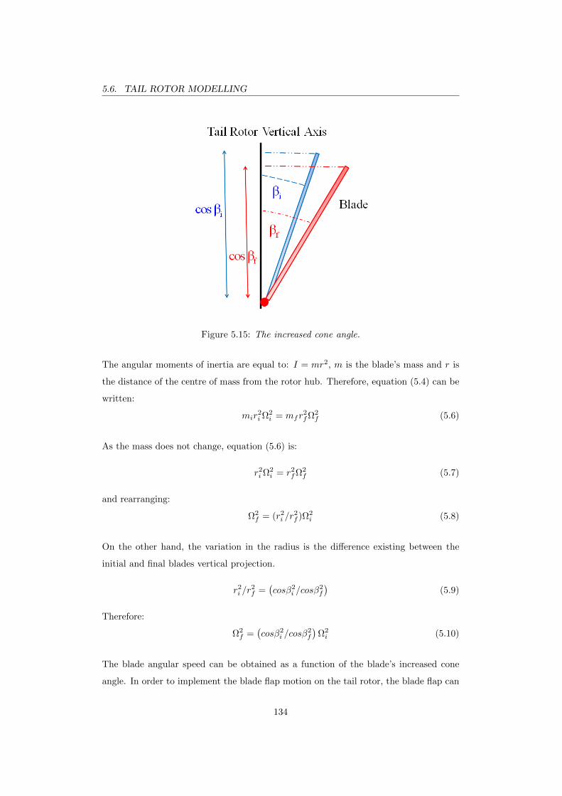
5.6. TAIL ROTOR MODELLING
Figure 5.15: The increased cone angle.
The angular moments of inertia are equal to: I = mr2, m is the blade’s mass and r is
the distance of the centre of mass from the rotor hub. Therefore, equation (5.4) can be
written:
mir2iΩ
2i = mfr
2fΩ2
f (5.6)
As the mass does not change, equation (5.6) is:
r2iΩ
2i = r2
fΩ2f (5.7)
and rearranging:
Ω2f = (r2
i /r2f )Ω2
i (5.8)
On the other hand, the variation in the radius is the difference existing between the
initial and final blades vertical projection.
r2i /r
2f =
(cosβ2
i /cosβ2f
)(5.9)
Therefore:
Ω2f =
(cosβ2
i /cosβ2f
)Ω2i (5.10)
The blade angular speed can be obtained as a function of the blade’s increased cone
angle. In order to implement the blade flap motion on the tail rotor, the blade flap can
134
5.6. TAIL ROTOR MODELLING
be defined as Fourier series [144]:
β = a0 − a1cosψf − b1sinψf (5.11)
where ψf = Ωf t, being Ωf the blade angular speed obtained as a function of the blade’s
cone angle (see equation (5.10)) and a0, a1, b1 are the corresponding Fourier coefficients.
(setsym fltl k "rq(fjtl k)")
(setsym wvr "(cos(aic)/cos(a0))*(krttl*omega)")
(setsym fltlref k "a0-a1*cos(@wvr*t)-b1*sin(@wvr*t)")
The first line provides the flap angle of the tail rotor blades. The second line defines the
blades’ rotational speed at the increased cone angle according to equation (5.10) where
the parameter krttl represents the tail rotor gearing, its numerical value is given in
Table 5.1 and aic is the initial cone angle. The third line, defines the flap angle on the
tail rotor as a Fourier series.
Once the flap reference signal has been defined, the PID controller can be implemented
by first defining the error variable:
(setsym fltlerror k "@fltlref k-@fltl k")
(add-state-variable fltltq k fltltqp k "F*L")
(set-aux-state-deriv fltltqp k "kifltl*@fltlerror k")
The add-state-variable command introduces a state variable for the moment ex-
pression. The integral part of the moment control is defined by set-aux-state-deriv
command and uses the value of the variable @fltlerror k defined above.
(add-moment ftlm k
:name "fjcttl k"
:direction [fjtl kx]
:body1 fjtl k
:body2 tailrt
:magnitude "fltltq k+kpfltl*(@fltlerror k)+kdfltl*dxdt(@fltlerror k)")
The controller uses the variable @fltlerror k as the input, and the output is the
moment applied to the blade flap hinges so that blade flap control is achieved. The
parameters kifltl, kpfltl and kdfltl are the integral, proportional and derivative
gains of the controller respectivelly.
135
5.6. TAIL ROTOR MODELLING
Feather Control Definition
Take blade one on the tail rotor, the feather angle control, the delta three angle structure
can be implemented by using a PID controller that constrains the blades’ position
around the tail rotor feather axis (Z). The feather control in this case is modelled as
follows:
(setsym ptlpj1 "rq(pj1tl)")
(setsym ptlref1 "fotl-tan(delta3tl)*rq(fj1tl)")
The first line creates a variable representing the first blade feather as rq(pj1tl). Then,
the variable @ptlref1 is defined, being the desired collective feather reference signal
fotl. The feather angle reduces its value by tan(delta3tl)*rq(fj1tl), as the conse-
quence of introducing the delta three angle.
(setsym ptlerror1 "@ptlref1-@ptlpj1")
(add-state-variable pl1tq tp1tqp "F*L")
(set-aux-state-deriv tp1tqp "kiptl*@ptlerror1")
add-state-variable introduces a state variable for the torque expression used to con-
trol the feather. The integral part of the torque is defined by set-aux-state-deriv
and uses the value of the @ptlerror1 defined above.
The expression to model this control moment is as follows:
(add-moment ptlm1
:name "pj1cttl"
:direction -[pjtl1z]
:body1 tailrt
:body2 pjtl1
:magnitude "pl1tq+kpptl*(@ptlerror1)+kdptl*dxdt(@ptlerror1)")
The torque is applied between the tail rotor and the first feather hinge. This controller
uses the variable @ptlerror1 as the input, and the output is the moment applied to
the first feather hinge so that collective control is achieved. kiptl, kpptl and kdptl
are the integral, proportional and derivative gains of the controller respectivelly.
136

5.6. TAIL ROTOR MODELLING
This was shown in here for the case of the tail rotor blade one; in the case of the blade
two, a similar moment was modelled and implemented in equal manner but in this case,
the direction of rotation around its local reference axis is just opposite (see Figure 5.16).
Figure 5.16: Tail rotor blades and the collective angle.
Tail Rotor Speed Control Modelling
As mentioned before, the tail rotor angular speed is proportional to the main rotor
angular speed [142]. Being this proportion the value of the tail rotor gearing krttl (see
Table 5.1).
The tail rotor rotational speed can be modelled as a constraint by using the VehicleSim
command ru(tailrt,1) which specifies the first rotational speed for the tail rotor:
(add-speed-constraint "ru(tailrt)-krttl*omega" :u "ru(tailrt)")
the value of the parameter krttl is defined at the beginning of the code.
On the other hand, the tail rotor speed can also be implemented by using a PID con-
troller in order to maintain a constant angular speed. In this case, the engine action
on the tail rotor can be modelled as a torque applied between the fuselage and the tail
rotor:
137

5.6. TAIL ROTOR MODELLING
(setsym wrotortl "ru(tailrt,1)")
(setsym wreftl "krttl*omega")
Two variables are defined, the first one, @wrotortl is the rotational speed of the tail
rotor around its Y axis and the second variable, @wreftl is the desired reference tail
rotor angular speed value.
(setsym werrortl "@wreftl-@wrotortl")
@werrortl is a variable that defines the existing error between the desired input angular
speed value @wreftl and the actual output angular speed, @wrotortl.
(add-state-variable wrttltq wrttltqp "F*L")
(set-aux-state-deriv wrttltqp "kirttl*@werrortl")
The add-state-variable introduces a new state variable. The integral part of the
controller is defined by set-aux-state-deriv and uses the value of the @werrortl
defined previously.
The expression of the moment applied in order to control the tail rotor speed is:
(add-moment tlcon
:name "Tail Torque"
:direction [tailrty]
:body1 fuselage
:body2 tailrt
:magnitude "wrttltq+kprttl*(@werrortl)+kdrttl*
dxdt(@werrortl)")
This controller uses the variable @werrortl as the input, and the output is the moment
applied to the tail rotor so that a desired rotational speed control is reached and sus-
tained. The variables kirttl, kprttl and kdrttl are the integral, proportional and
derivative gains of the controller respectivelly.
138
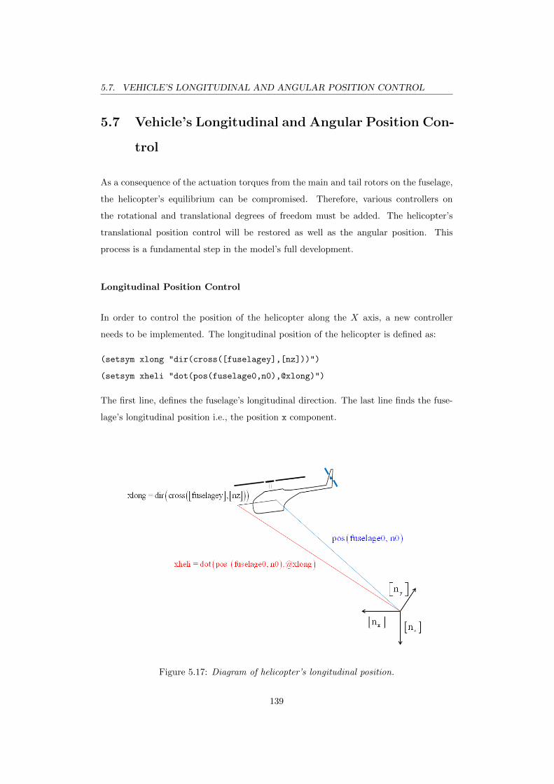
5.7. VEHICLE’S LONGITUDINAL AND ANGULAR POSITION CONTROL
5.7 Vehicle’s Longitudinal and Angular Position Con-
trol
As a consequence of the actuation torques from the main and tail rotors on the fuselage,
the helicopter’s equilibrium can be compromised. Therefore, various controllers on
the rotational and translational degrees of freedom must be added. The helicopter’s
translational position control will be restored as well as the angular position. This
process is a fundamental step in the model’s full development.
Longitudinal Position Control
In order to control the position of the helicopter along the X axis, a new controller
needs to be implemented. The longitudinal position of the helicopter is defined as:
(setsym xlong "dir(cross([fuselagey],[nz]))")
(setsym xheli "dot(pos(fuselage0,n0),@xlong)")
The first line, defines the fuselage’s longitudinal direction. The last line finds the fuse-
lage’s longitudinal position i.e., the position x component.
Figure 5.17: Diagram of helicopter’s longitudinal position.
139

5.7. VEHICLE’S LONGITUDINAL AND ANGULAR POSITION CONTROL
(setsym xref "x ref")
The variable @xref is added, as the reference value for the fuselage’s longitudinal posi-
tion. It is defined as a numerical value in this case zero because the equilibrium position
(point (0, 0, 0)) should remain. In the next chapters, this variable will be an equation
to allow for longitudinal trajectory prescription.
(setsym xerror "@xref-@xheli")
(add-state-variable xfutq xfutqp "F")
(set-aux-state-deriv xfutqp "kix*@xerror")
The add-state-variable introduces a state variable for the force expression used to
control the helicopter’s longitudinal position. The integral part of the force is defined
with the set-aux-state-deriv and uses the value of the @xerror defined as the dif-
ference between the actual and desired helicopter longitudinal position.
(add-line-force xcon
:name "xctrl"
:direction [fuselagex]
:point1 fuselage0
:point2 n0
:magnitude "xfutq+kpx*(@xerror)+kdx*dxdt(@xerror)")
The force is applied between the fuselage (fuselage’s centre fuselage0) and the inertial
frame. The controller uses the variable @xerror as the input variable and the output is
the force applied to the fuselage, so a desired longitudinal position control is achieved.
The parameters kix, kpx and kdx are the gains of the controller.
The lateral and vertical position controls are modelled similarly to the longitudinal
position control and therefore are not included in this report.
Fuselage’s Yaw Control
In order to control the helicopter’s yaw (rotation around the Z axis), a new controller
is added. The yaw is calculated as:
(setsym phifusez "rq(fuselage,1)")
140
5.8. CHAPTER SUMMARY
where rq(fuselage,1) specifies the fuselage’s first rotational coordinate.
(setsym phirefz "fuszref")
The variable @phirefz is defined as the reference value for the fuselage’s yaw. It is
defined as a zero because the equilibrium position should be restored. Its numerical
value is defined at the beginning of the program. In the following chapters, this variable
will be an equation that allows to describe a yaw helicopter trajectory in the space.
(setsym phierrorz "@phirefz-@phifusez")
(add-state-variable fuseztq fuseztqp "F*L")
(set-aux-state-deriv fuseztqp "kifsz*@phierrorz")
The add-state-variable introduces a state variable for the torque expression that it
is used to control the helicopter yaw. The integral part of the torque is defined with the
set-aux-state-deriv and uses the value of the phierrorz defined above. @phierrorz
is the difference between the actual and desired fuselage’s yaw.
(add-moment fszphi
:name "phictrlz"
:direction -[fuselagez]
:body1 fuselage
:body2 n
:magnitude "fuseztq+kpfsz*(@phierrorz)+kdfsz*dxdt(@phierrorz)")
The torque is applied between the fuselage and the inertial frame. The controller uses
the variable @phierrorz as the input variable and the output is the torque applied
to the fuselage adequate yaw control is achieved. The parameters kifsz, kpfsz and
kdfsz are the gains of the controller.
The pitch and roll control are modelled similarly to the yaw control.
5.8 Chapter Summary
The aim of this chapter was to provide a model of a helicopter by using the multibody
modelling code VehicleSim. The derived model has been developed without the influence
of external forces i.e., the system is considered to be in vacuum. As it has been shown,
141
5.8. CHAPTER SUMMARY
the fuselage, the main rotor and tail rotor have been built by using the parent-child
structure dictated by VehicleSim. In addition to this, the connections between the
several bodies have been represented and the degrees of freedom for each body have
been modelled.
The procedure for modelling the main rotor consisted of defining a body composed by
several hinges as well as flap, lag and feather degrees of freedom. The blades are added
as bodies with mass and inertial properties, and they are rigid. The actions of the
swashplate on the blades were simulated implementing various PID controllers, so the
blades’ motions on the disc plane can be simulated together with the flap and lag hinges.
The collective and cyclic feather control has been designed and modelled.
Additionally, the speed ratio between the mail and the tail rotors has been set up, as
well as the effects the engine has on the fuselage. The delta three angle and its effects
on the tail rotor has been modelled. It is worthy of note that the coupling existing
between the flap and the feather degree of freedom on the tail rotor has been explained
carefully in order to understand this complex effect. This allowed the next stage in the
modelling process as the feather collective was designed and modelled according to the
delta three implementation.
Various PID controllers are included to achieve position and rotation equilibrium. The
modelling for longitudinal position control as well as yaw control were carefully de-
scribed. Taking into account the previous considerations, the control of the helicopter
around the equilibrium point (0, 0, 0) is obtained, getting the desired equilibrium when
both main and tail torques operate on the system.
Overall, this model here presented captures nonlinear dynamics and couplings existing
in a complex mechanical system such as a helicopter.
The following chapters will explore further the nature of these couplings, their mathe-
matical representations, their implications on the vehicle’s behaviour and their physical
impact on the blade’s and fuselage’s degrees of freedom in the absence of an aerodynamic
environment. In the last chapters of this thesis, the problem of adding aerodynamic
forces on this model is also treated.
142
Chapter 6
External Perturbations
Modelling for Sikorsky Model
(Aerodynamic Model)
6.1 Introduction
The main aim of this chapter is to describe the modelling developed for analyzing the
external perturbations on the helicopter dynamics model described in Chapter 5. First,
gravity is added to the system, so the equilibrium on the vehicle under the action of this
force should be restored. The ground is also simulated on the helicopter. After that,
the inclination on the main rotor is considered in order to build up a helicopter model
close to a real model as well as to study the impact this inclination has on the system
when the aerodynamic forces are included. On the other hand, the model is enhanced
by modelling varying rotating speed on the main rotor. Finally, an aerodynamic model
is presented for both main and tail rotors, the fuselage’s aerodynamic effects are not
considered, this task will be developed in the near future by the author, the aerodynamic
modelling is focused on both rotors using blade element theory.
143
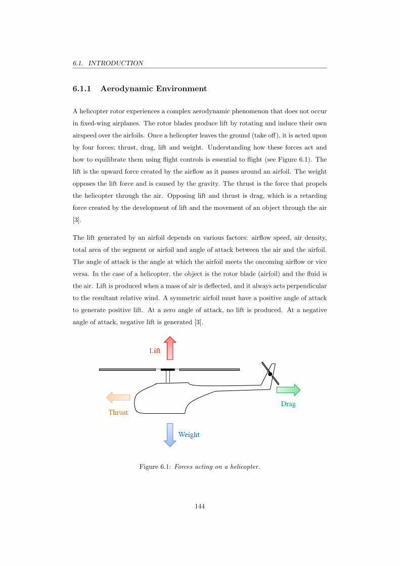
6.1. INTRODUCTION
6.1.1 Aerodynamic Environment
A helicopter rotor experiences a complex aerodynamic phenomenon that does not occur
in fixed-wing airplanes. The rotor blades produce lift by rotating and induce their own
airspeed over the airfoils. Once a helicopter leaves the ground (take off), it is acted upon
by four forces; thrust, drag, lift and weight. Understanding how these forces act and
how to equilibrate them using flight controls is essential to flight (see Figure 6.1). The
lift is the upward force created by the airflow as it passes around an airfoil. The weight
opposes the lift force and is caused by the gravity. The thrust is the force that propels
the helicopter through the air. Opposing lift and thrust is drag, which is a retarding
force created by the development of lift and the movement of an object through the air
[3].
The lift generated by an airfoil depends on various factors: airflow speed, air density,
total area of the segment or airfoil and angle of attack between the air and the airfoil.
The angle of attack is the angle at which the airfoil meets the oncoming airflow or vice
versa. In the case of a helicopter, the object is the rotor blade (airfoil) and the fluid is
the air. Lift is produced when a mass of air is deflected, and it always acts perpendicular
to the resultant relative wind. A symmetric airfoil must have a positive angle of attack
to generate positive lift. At a zero angle of attack, no lift is produced. At a negative
angle of attack, negative lift is generated [3].
Figure 6.1: Forces acting on a helicopter.
144
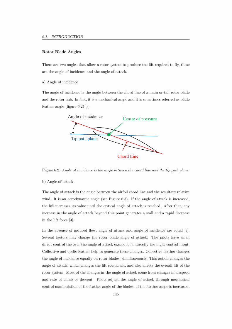
6.1. INTRODUCTION
Rotor Blade Angles
There are two angles that allow a rotor system to produce the lift required to fly, these
are the angle of incidence and the angle of attack.
a) Angle of incidence
The angle of incidence is the angle between the chord line of a main or tail rotor blade
and the rotor hub. In fact, it is a mechanical angle and it is sometimes referred as blade
feather angle (figure 6.2) [3].
Figure 6.2: Angle of incidence is the angle between the chord line and the tip path plane.
b) Angle of attack
The angle of attack is the angle between the airfoil chord line and the resultant relative
wind. It is an aerodynamic angle (see Figure 6.3). If the angle of attack is increased,
the lift increases its value until the critical angle of attack is reached. After that, any
increase in the angle of attack beyond this point generates a stall and a rapid decrease
in the lift force [3].
In the absence of induced flow, angle of attack and angle of incidence are equal [3].
Several factors may change the rotor blade angle of attack. The pilots have small
direct control the over the angle of attack except for indirectly the flight control input.
Collective and cyclic feather help to generate these changes. Collective feather changes
the angle of incidence equally on rotor blades, simultaneously. This action changes the
angle of attack, which changes the lift coefficient, and also affects the overall lift of the
rotor system. Most of the changes in the angle of attack come from changes in airspeed
and rate of climb or descent. Pilots adjust the angle of attack through mechanical
control manipulation of the feather angle of the blades. If the feather angle is increased,
145
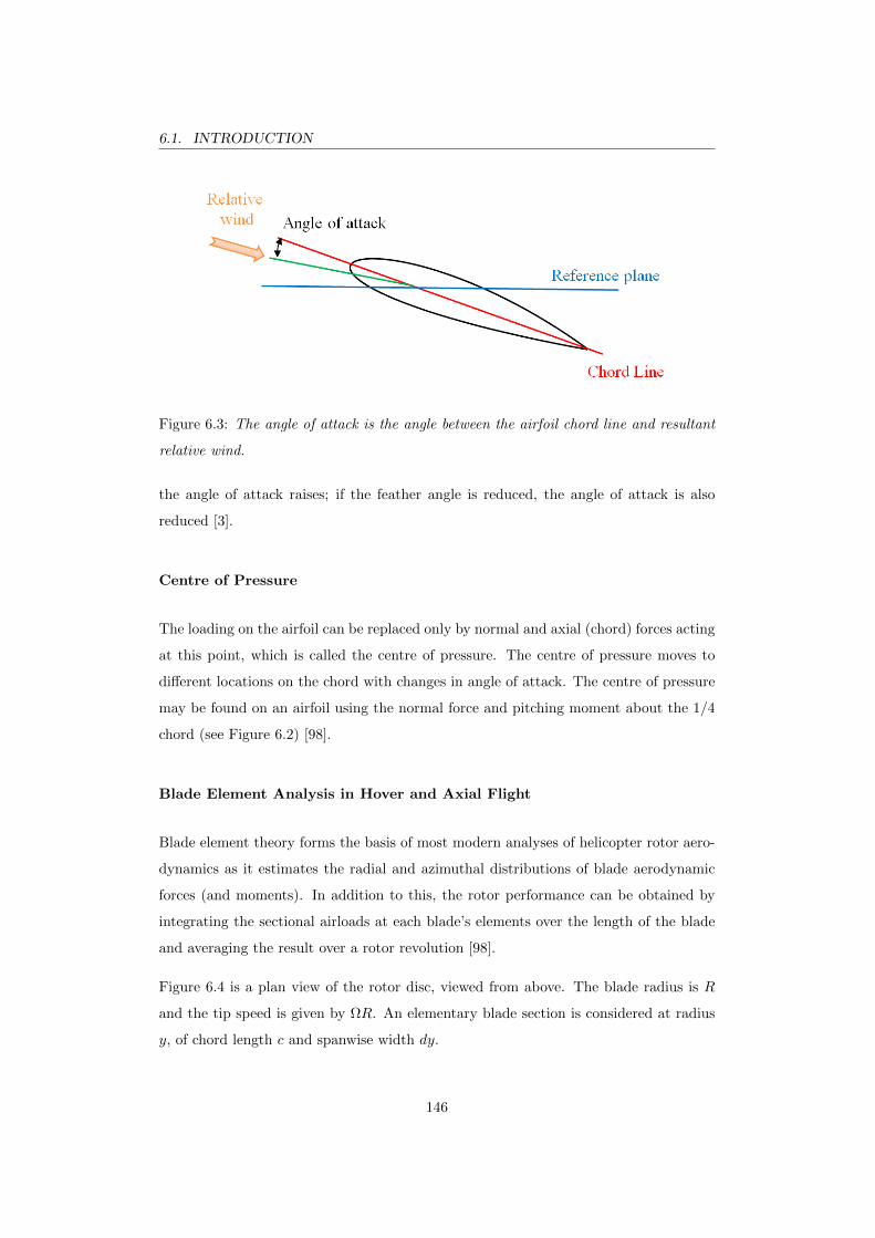
6.1. INTRODUCTION
Figure 6.3: The angle of attack is the angle between the airfoil chord line and resultant
relative wind.
the angle of attack raises; if the feather angle is reduced, the angle of attack is also
reduced [3].
Centre of Pressure
The loading on the airfoil can be replaced only by normal and axial (chord) forces acting
at this point, which is called the centre of pressure. The centre of pressure moves to
different locations on the chord with changes in angle of attack. The centre of pressure
may be found on an airfoil using the normal force and pitching moment about the 1/4
chord (see Figure 6.2) [98].
Blade Element Analysis in Hover and Axial Flight
Blade element theory forms the basis of most modern analyses of helicopter rotor aero-
dynamics as it estimates the radial and azimuthal distributions of blade aerodynamic
forces (and moments). In addition to this, the rotor performance can be obtained by
integrating the sectional airloads at each blade’s elements over the length of the blade
and averaging the result over a rotor revolution [98].
Figure 6.4 is a plan view of the rotor disc, viewed from above. The blade radius is R
and the tip speed is given by ΩR. An elementary blade section is considered at radius
y, of chord length c and spanwise width dy.
146

6.1. INTRODUCTION
Figure 6.4: Main rotor disc viewed from above. This figure is plotted by the author and
based on [145].
The forces on the blade’s section are shown in Figure 6.5. The flow seen by the section
has velocity components Ωy in the disc plane and (vi + Vc) (vi is the induced velocity
and Vc is the upward velocity) perpendicular to it [145].
Figure 6.5: Flow conditions in vertical flight for a blade section. This figure is drawn
by the author and based on [145].
The resultant local flow velocity at any blade element at a radial distance y from the
rotational axis has an out of plane component UP = (vi +Vc) normal to the rotor plane
as a result of climb and induced inflow and an in plane component UT = Ωy parallel to
the rotor due to the blade rotation, relative to the disc plane. The resultant velocity at
the blade element is therefore the composition of both [98]:
147
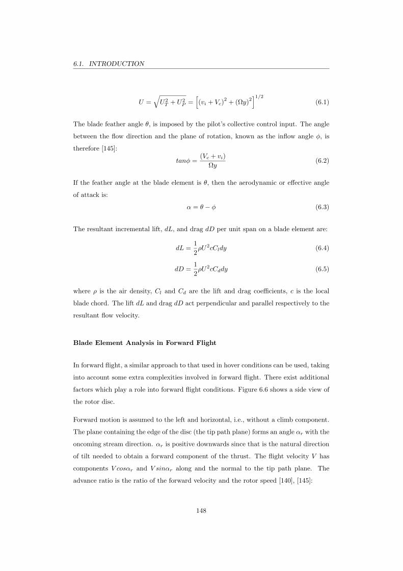
6.1. INTRODUCTION
U =√U2T + U2
P =[(vi + Vc)
2+ (Ωy)
2]1/2
(6.1)
The blade feather angle θ, is imposed by the pilot’s collective control input. The angle
between the flow direction and the plane of rotation, known as the inflow angle φ, is
therefore [145]:
tanφ =(Vc + vi)
Ωy(6.2)
If the feather angle at the blade element is θ, then the aerodynamic or effective angle
of attack is:
α = θ − φ (6.3)
The resultant incremental lift, dL, and drag dD per unit span on a blade element are:
dL =1
2ρU2cCldy (6.4)
dD =1
2ρU2cCddy (6.5)
where ρ is the air density, Cl and Cd are the lift and drag coefficients, c is the local
blade chord. The lift dL and drag dD act perpendicular and parallel respectively to the
resultant flow velocity.
Blade Element Analysis in Forward Flight
In forward flight, a similar approach to that used in hover conditions can be used, taking
into account some extra complexities involved in forward flight. There exist additional
factors which play a role into forward flight conditions. Figure 6.6 shows a side view of
the rotor disc.
Forward motion is assumed to the left and horizontal, i.e., without a climb component.
The plane containing the edge of the disc (the tip path plane) forms an angle αr with the
oncoming stream direction. αr is positive downwards since that is the natural direction
of tilt needed to obtain a forward component of the thrust. The flight velocity V has
components V cosαr and V sinαr along and the normal to the tip path plane. The
advance ratio is the ratio of the forward velocity and the rotor speed [140], [145]:
148
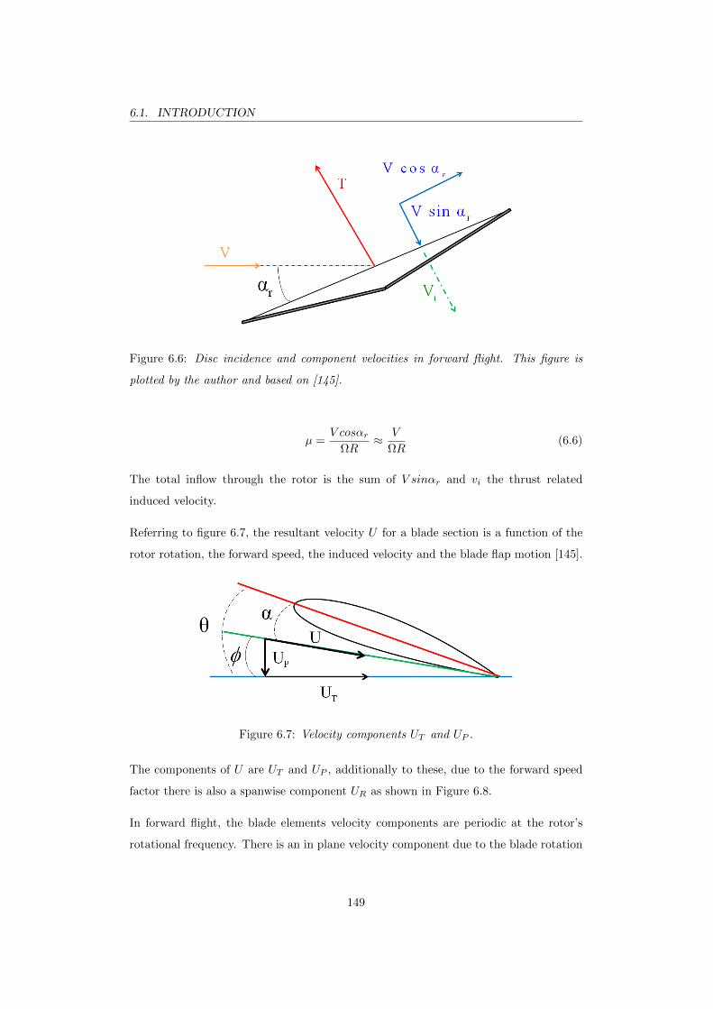
6.1. INTRODUCTION
Figure 6.6: Disc incidence and component velocities in forward flight. This figure is
plotted by the author and based on [145].
µ =V cosαr
ΩR≈ V
ΩR(6.6)
The total inflow through the rotor is the sum of V sinαr and vi the thrust related
induced velocity.
Referring to figure 6.7, the resultant velocity U for a blade section is a function of the
rotor rotation, the forward speed, the induced velocity and the blade flap motion [145].
Figure 6.7: Velocity components UT and UP .
The components of U are UT and UP , additionally to these, due to the forward speed
factor there is also a spanwise component UR as shown in Figure 6.8.
In forward flight, the blade elements velocity components are periodic at the rotor’s
rotational frequency. There is an in plane velocity component due to the blade rotation
149
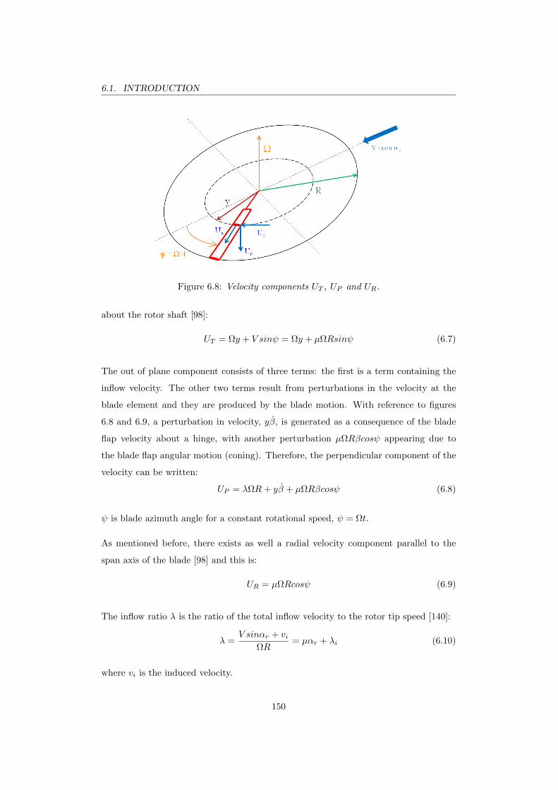
6.1. INTRODUCTION
Figure 6.8: Velocity components UT , UP and UR.
about the rotor shaft [98]:
UT = Ωy + V sinψ = Ωy + µΩRsinψ (6.7)
The out of plane component consists of three terms: the first is a term containing the
inflow velocity. The other two terms result from perturbations in the velocity at the
blade element and they are produced by the blade motion. With reference to figures
6.8 and 6.9, a perturbation in velocity, yβ, is generated as a consequence of the blade
flap velocity about a hinge, with another perturbation µΩRβcosψ appearing due to
the blade flap angular motion (coning). Therefore, the perpendicular component of the
velocity can be written:
UP = λΩR+ yβ + µΩRβcosψ (6.8)
ψ is blade azimuth angle for a constant rotational speed, ψ = Ωt.
As mentioned before, there exists as well a radial velocity component parallel to the
span axis of the blade [98] and this is:
UR = µΩRcosψ (6.9)
The inflow ratio λ is the ratio of the total inflow velocity to the rotor tip speed [140]:
λ =V sinαr + vi
ΩR= µαr + λi (6.10)
where vi is the induced velocity.
150

6.1. INTRODUCTION
Figure 6.9: Perturbation velocities on the blade resulting from blade flap velocity and
rotor coning. This figure is plotted by the author and based on [98].
For helicopter rotors the following assumptions can be made:
• The out of plane velocity UP is smaller than the in plane velocity UT , so that
U =√U2T + U2
P ≈ UT . This is a valid approximation except near the blade root,
but the aerodynamic forces are small here anyway.
• The induced angle φ, is small, so that φ = UP /UT [98].
As a result of these approximations, the blade angle of incidence may now be written
as:
α = θ − φ = θ − UPUT
(6.11)
The resultant incremental lift dL per unit span on the blade element is now:
dL =1
2ρU2cCldy (6.12)
and similarly the incremental drag is:
dD =1
2ρU2cCddy (6.13)
which act perpendicular and parallel to the resultant flow velocity at the blade section.
151
6.2. EARTH/GROUND MODELLING
6.2 Earth/Ground Modelling
The first external force that it is included on the model script derived in this work is the
gravity force. The helicopter simulation model is subjected to an unbalance of forces
that should be taken into account in order to restore the equilibrium.
First, gravity is added by the command:
(add-gravity)
Taking into account third Newton’s law on the fuselage i.e., the gravity force acts in the
vertical downwards direction whereas the earth/ground exerts a force with opposite di-
rection (reaction) an equal magnitude. As a result, a vertical force should be introduced
in the model:
(setsym z long "dir(cross([fuselagex],[ny]))")
(setsym hheli "dot(pos(fuselage0,n0),@z long)")
The first line, defines the vertical direction of the fuselage. The second line finds the
exact fuselage vertical position i.e., the z position component.
The magnitude of the ground reaction is modelled as follows:
(setsym Fzm "kgrsp*(rg-@hheli)+kgrd*dxdt(rg-@hheli)")
where kgrsp and kgrd are constant values defined at the beginning of the program.
They are the values of a spring and damper modelled to help to simulate the ground
reaction to gravity. The ground force on the helicopter is modelled under the action of
a spring and damper to allow changes in the force when the helicopter’s mass changes.
For example, if an additional load is needed (cargo, etc) the new helicopter’s weight and
ground force are calibrated by changing the spring constant and damping coefficient.
Finally, rg is the reference value for the ground i.e., zero.
The command add-line-force introduces a normal force on the fuselage with a mag-
nitude defined by the variable @Fzm in opposite direction to the gravity force.
152
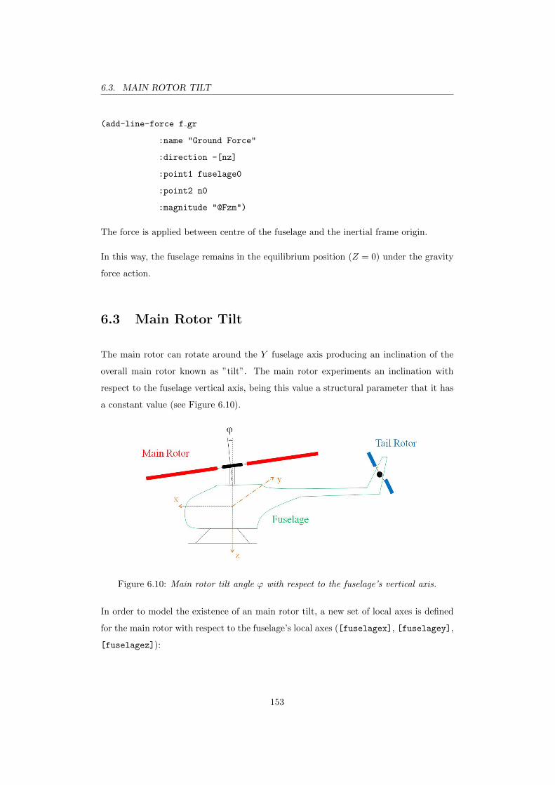
6.3. MAIN ROTOR TILT
(add-line-force f gr
:name "Ground Force"
:direction -[nz]
:point1 fuselage0
:point2 n0
:magnitude "@Fzm")
The force is applied between centre of the fuselage and the inertial frame origin.
In this way, the fuselage remains in the equilibrium position (Z = 0) under the gravity
force action.
6.3 Main Rotor Tilt
The main rotor can rotate around the Y fuselage axis producing an inclination of the
overall main rotor known as ”tilt”. The main rotor experiments an inclination with
respect to the fuselage vertical axis, being this value a structural parameter that it has
a constant value (see Figure 6.10).
Figure 6.10: Main rotor tilt angle ϕ with respect to the fuselage’s vertical axis.
In order to model the existence of an main rotor tilt, a new set of local axes is defined
for the main rotor with respect to the fuselage’s local axes ([fuselagex], [fuselagey],
[fuselagez]):
153
6.3. MAIN ROTOR TILT
(setsym rt inclx "cos(ang)*[fuselagex]+sin(ang)*[fuselagez]")
(setsym rt incly "[fuselagey]")
(setsym rt inclz "-sin(ang)*[fuselagex]+cos(ang)*[fuselagez]")
ang is the tilt angle, its value is constant and it is defined at the beginning of the
program.
A point in the helicopter nominal configuration within the coordinate system of body
n needs to be defined to connect the rotor to the fuselage at the point fsg.
(add-point fsgp :body n :coordinates (0 0 -h))
(add-point fsg :body fuselage :coordinates fsgp)
The point fsg is located at a vertical distance -h from the origin of the inertial axes
system.
The main rotor is introduced in the model as follows:
(add-body rt
:name "Rotor"
:parent fuselage
:mass 0
:joint-coordinates fsg
:body-rotation-axes z
:parent-rotation-axis "@rt inclz"
:reference-axis "@rt inclx"
:inertia-matrix (0 0 Irt z))
The rotor has the fuselage as parent. It is set up as a massless body. The rotational
degree of freedom around the rotor’s Z axes is considered and takes into account the
new axes defined as tilted with respect to the fuselage (see ”@rt inclz” defined as the
parent-rotation-axis). The coordinates of the joint between the main rotor and the
fuselage are given by the command: joint-coordinates, its numerical value is defined
by the point fsg. Finally, its moments of inertia are provided.
154

6.4. MAIN ROTOR VARYING ANGULAR SPEED
6.4 Main Rotor Varying Angular Speed
The main rotor angular speed in this model, makes use of a PID controller in order to
change the angular speed according to some specific demand. This is dictated by the
expression: Ω(t) = 2πf1 +2πf2cos (2πf3t) where f1, f2 and f3 are frequencies expressed
in Hz [93]. A torque between the fuselage and the main rotor will be introduced as means
to change the angular speed.
(setsym wrotor "ru(rt,1)")
(setsym wref "(2*@pi*f1)+(2*@pi*f2)*cos(2*@pi*f3*t)+acce*t")
Two variables are defined, the first one, @wrotor is the angular speed of the main rotor
around the Z axis and the second variable, @wref, is the reference value of the angular
speed of the main rotor. As it can be seen, three parameters need to be defined, f1,
f2, f3, the corresponding frequency values. The first one represents the main rotor
angular speed, the second and third introduce a variation on the main rotor angular
speed. Their numerical values are defined at the beginning of the program. Also, an
acceleration value, acce, is introduced so the targeted main rotor angular speed can be
reached gradually in a realistic manner, as acce*t appears on the variable @wref.
add-state-variable introduces a state variable for the torque expression that will
dictate the main rotor speed. The integral part of the torque is defined by the
set-aux-state-deriv command and uses the value of @werror.
(setsym werror "@wref-@wrotor")
(add-state-variable wrttq wrttqp "F*L")
(set-aux-state-deriv wrttqp "ki*@werror")
(add-moment rtcon
:name "Rotor Torque"
:direction [rtz]
:body1 fuselage
:body2 rt
:magnitude "wrttq+kp*(@werror)+kd*dxdt(@werror)")
This controller uses the variable @werror as the input and the output is the moment
applied to the main rotor so that main rotor angular speed control is achieved. The
155
6.5. MAIN ROTOR AERODYNAMIC MODELLING
variables ki, kp and kd are the gains of the controller that can be adjusted without
the need of new compilation.
6.5 Main Rotor Aerodynamic Modelling
In order to model the aerodynamic environment, in this section, fundamental concepts
such as air density, induced speeds, lift and drag forces, thrust coefficients are intro-
duced.
6.5.1 Air Density
In every flight condition, the air density changes with the height (h), for the lower
atmosphere where helicopters fly below 6000 m, the standard value of air density can
be approximated as [98]:
ρ = ρ0e−0.0296h/304.8 (6.14)
where h is expressed in meters and ρ0 = 1.225 kg/m3.
The previous expression is implemented in VehicleSim as:
(setsym ro air "rho*(exp((-0.0296*abs(tq(fuselage,3)))/304.8))")
the height is given by the fuselage’s vertical position tq(fuselage,3). This expression
provides the air density value for all the height range reached by the helicopter.
6.5.2 Induced Hover Speed
In hovering flight, the induced velocity can be obtained according to the expression
vi = vi0, vi0 is the hover induced velocity, which can be considered constant in hover,
the traction force, T , becomes equal to the disc loading (weight of the helicopter) [98]:
vi0 =
√T
2ρπR2(6.15)
The induced hover velocity is implemented in VehicleSim as follows:
156
6.5. MAIN ROTOR AERODYNAMIC MODELLING
(setsym vih "sqrt(((mf+mbl1+mbl2+mbl3+mbl4+mbl tl1+mbl tl2)*g)/
(2*@ro air*@pi*Rt**2)))")
the traction force, magnitude T , is equal to weight of the helicopter, where mf is the
fuselage mass, mbl1, mbl2, mbl3, mbl4 are the main rotor blades’ masses. mbl tl1,
mbl tl2 are the tail rotor blades’ masses. @ro air is the air density and Rt is the main
rotor radius.
6.5.3 Climb, Descent and Forward Speed
Climb Velocity
The climb velocity can be modelled as a function of the induced velocity in hover:
(setsym vc "cteclimb*(Kclimb*@vih)")
where cteclimb is a boolean parameter that will allow to choose one from the different
options of flight such as hover, climb, descent and forward flight, all of them are modelled
in the same code. In order to simulate this, one of the boolean parameters takes the
value one for the corresponding flight condition and the rest of them remain null. The
parameter Kclimb is the ratio between the climb velocity and the induced hover velocity,
it will be defined by using several theoretical considerations. Finally, @vih is the variable
representing the induced hover velocity.
Descent Velocity
The descent velocity is implemented as:
(setsym vdes "ctevid*(ctdesc*@vih)")
ctevid is the corresponding boolean parameter. The value ctdesc is the ratio between
the descent velocity and the induced hover velocity. It is obtained by taking into account
the theoretical approach and @vih is the variable represented the induced hover velocity.
157
6.5. MAIN ROTOR AERODYNAMIC MODELLING
Forward Velocity
The forward velocity expression is given by:
V =µΩR
cos(αr)(6.16)
µ is the advance ratio, Ω is the rotor angular speed, R is the rotor radius and αr is
assumed positive downwards since that is the natural direction of the tilt needed to
obtain a forward component of the thrust.
According to this, the forward velocity can be modelled as:
(setsym vheli "(mu*Rt*@wrotor)/cos((ktray1*gamma)+(ktray2*@phi fusey))")
mu is the advance ratio, its value is defined at the beginning of the program. Rt is the
main rotor radius. @wrotor is the main rotor angular speed. Two boolean variables are
defined, ktray1 and ktray2, they allow to consider the natural direction of tilt. For a
constant tilt, gamma is indicated, its numerical value is defined at the beginning of the
program. On the other hand, for a variable tilt @phi fusey, indicates the fuselage’s
pitch.
6.5.4 Induced Climb, Descent and Forward Velocities
Induced Climb Velocity
The induced climb velocity is proportional to the induced hover speed, as Figure 6.11
shows [98]. The induced climb velocity in vertical flight is then implemented as:
(setsym viclmb "ctecli*(cteviclmb*(@vih))")
ctecli is a boolean parameter, cteviclmb is the parameter that provides the propor-
tional value between both speeds. The variable @vih is the induced hover velocity.
Induced Descent Velocity
In vertical descent, the air flow through the rotor undergoes significant changes. The
stream velocity, Vc, is now negative whilst the induced velocity remains positive as the
rotor maintains the lift.
158
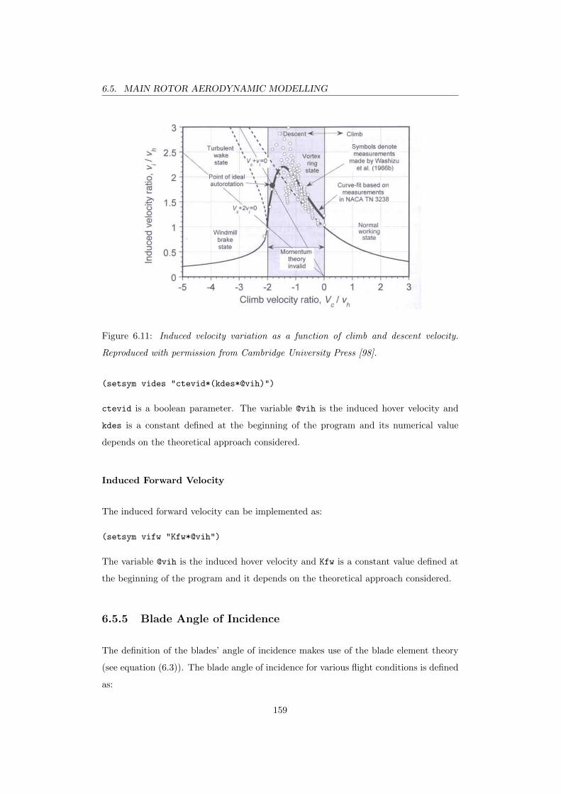
6.5. MAIN ROTOR AERODYNAMIC MODELLING
Figure 6.11: Induced velocity variation as a function of climb and descent velocity.
Reproduced with permission from Cambridge University Press [98].
(setsym vides "ctevid*(kdes*@vih)")
ctevid is a boolean parameter. The variable @vih is the induced hover velocity and
kdes is a constant defined at the beginning of the program and its numerical value
depends on the theoretical approach considered.
Induced Forward Velocity
The induced forward velocity can be implemented as:
(setsym vifw "Kfw*@vih")
The variable @vih is the induced hover velocity and Kfw is a constant value defined at
the beginning of the program and it depends on the theoretical approach considered.
6.5.5 Blade Angle of Incidence
The definition of the blades’ angle of incidence makes use of the blade element theory
(see equation (6.3)). The blade angle of incidence for various flight conditions is defined
as:
159
6.5. MAIN ROTOR AERODYNAMIC MODELLING
Hover:
α = θ − arctan
(vihΩy
)(6.17)
Climbing flight:
α = θ − arctan
(Vc + vic
Ωy
)(6.18)
Descent flight:
α = θ − arctan
(Vdes + vid
Ωy
)(6.19)
Forward flight:
α = θ −(UPUT
)(6.20)
In VehicleSim, the angle of incidence for forward flight is implemented by using equation
(6.7). UT is modelled as:
(setsym ut i "(omega*(y i+eR))+(omega*Rt*mu*sin(@wrotor*t))")
for i = 1, .., 3. i is the corresponding point on the blade where the aerodynamic load is
applied to.
By using equation (6.8), UP is:
(setsym up j i "(@wrotor*Rt*@lambda)+(@wrotor*Rt*mu*cos(@wrotor*t)*
rq(fj j))+((y i+eR)*dxdt(rq(fj j)))")
where j = 1, .., 4 (j is number of blades) and i = 1, .., 3.
Taking into account equations (6.11) and (6.17 - 6.19) the total angle of incidence for
hover, climb and descent/forward fight can be implemented as:
(setsym alpha j i "rq(pj j)-atan(((ctecl*(@vc+@viclmb))/(omega*(y i+eR)))
+((ctvids*(@vdes+@vides))/(omega*(y i+eR)))+((ctehv*@vih)/(omega*(y i+
eR))))+((ctefw*@up j i)/@ut i)")
where rq(pj j) is the feather angle of each blade. ctecl, ctvids, ctehv and ctefw
are boolean variables, they allow to choose the corresponding flight condition on each
case by setting one of them to 1 and letting the rest of them as 0. y i is the distance
along the blade’s Y axis where the angle of incidence is measured (see Figure 6.12). In
order to solve the error that VehicleSim provides when the variable @wrotor is used as
160
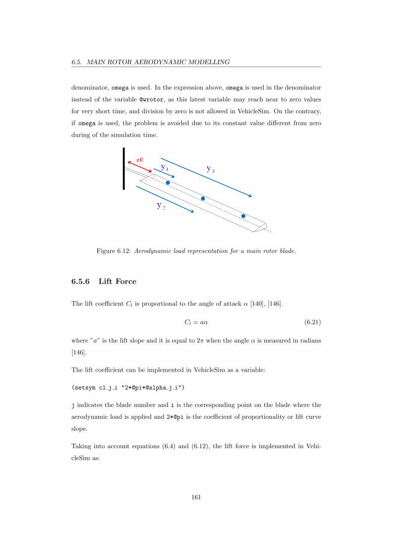
6.5. MAIN ROTOR AERODYNAMIC MODELLING
denominator, omega is used. In the expression above, omega is used in the denominator
instead of the variable @wrotor, as this latest variable may reach near to zero values
for very short time, and division by zero is not allowed in VehicleSim. On the contrary,
if omega is used, the problem is avoided due to its constant value different from zero
during of the simulation time.
Figure 6.12: Aerodynamic load representation for a main rotor blade.
6.5.6 Lift Force
The lift coefficient Cl is proportional to the angle of attack α [140], [146].
Cl = aα (6.21)
where ”a” is the lift slope and it is equal to 2π when the angle α is measured in radians
[146].
The lift coefficient can be implemented in VehicleSim as a variable:
(setsym cl j i "2*@pi*@alpha j i")
j indicates the blade number and i is the corresponding point on the blade where the
aerodynamic load is applied and 2*@pi is the coefficient of proportionality or lift curve
slope.
Taking into account equations (6.4) and (6.12), the lift force is implemented in Vehi-
cleSim as:
161
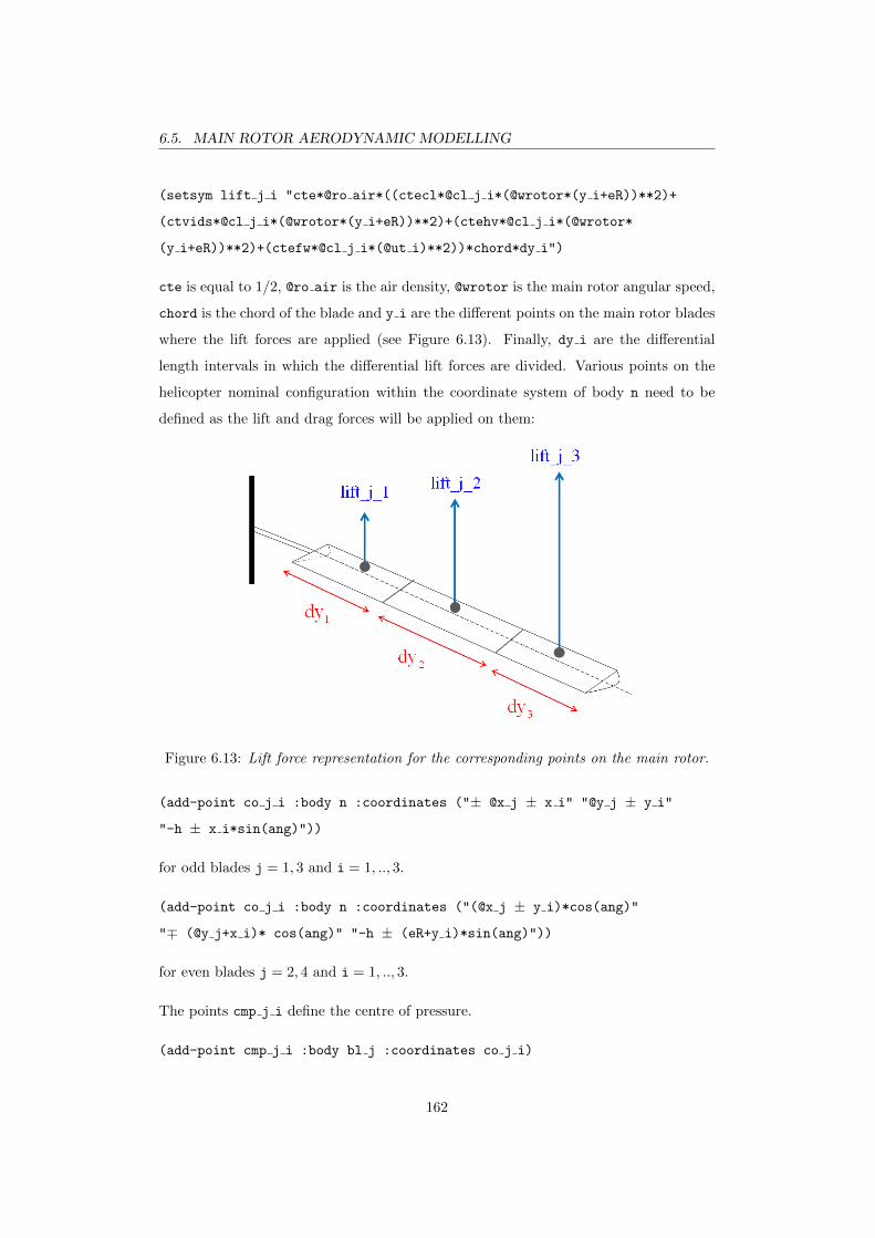
6.5. MAIN ROTOR AERODYNAMIC MODELLING
(setsym lift j i "cte*@ro air*((ctecl*@cl j i*(@wrotor*(y i+eR))**2)+
(ctvids*@cl j i*(@wrotor*(y i+eR))**2)+(ctehv*@cl j i*(@wrotor*
(y i+eR))**2)+(ctefw*@cl j i*(@ut i)**2))*chord*dy i")
cte is equal to 1/2, @ro air is the air density, @wrotor is the main rotor angular speed,
chord is the chord of the blade and y i are the different points on the main rotor blades
where the lift forces are applied (see Figure 6.13). Finally, dy i are the differential
length intervals in which the differential lift forces are divided. Various points on the
helicopter nominal configuration within the coordinate system of body n need to be
defined as the lift and drag forces will be applied on them:
Figure 6.13: Lift force representation for the corresponding points on the main rotor.
(add-point co j i :body n :coordinates ("± @x j ± x i" "@y j ± y i"
"-h ± x i*sin(ang)"))
for odd blades j = 1, 3 and i = 1, .., 3.
(add-point co j i :body n :coordinates ("(@x j ± y i)*cos(ang)"
"∓ (@y j+x i)* cos(ang)" "-h ± (eR+y i)*sin(ang)"))
for even blades j = 2, 4 and i = 1, .., 3.
The points cmp j i define the centre of pressure.
(add-point cmp j i :body bl j :coordinates co j i)
162
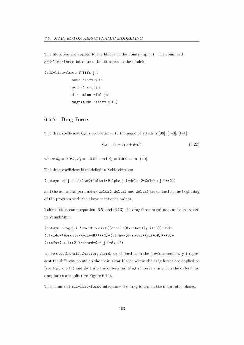
6.5. MAIN ROTOR AERODYNAMIC MODELLING
The lift forces are applied to the blades at the points cmp j i. The command
add-line-force introduces the lift forces in the model:
(add-line-force f lift j i
:name "lift j i"
:point1 cmp j i
:direction -[bl jz]
:magnitude "@lift j i")
6.5.7 Drag Force
The drag coefficient Cd is proportional to the angle of attack α [98], [140], [141]:
Cd = d0 + d1α+ d2α2 (6.22)
where d0 = 0.087, d1 = −0.021 and d2 = 0.400 as in [140].
The drag coefficient is modelled in VehicleSim as:
(setsym cd j i "delta0+delta1*@alpha j i+delta2*@alpha j i**2")
and the numerical parameters delta0, delta1 and delta2 are defined at the beginning
of the program with the above mentioned values.
Taking into account equation (6.5) and (6.13), the drag force magnitude can be expressed
in VehicleSim:
(setsym drag j i "cte*@ro air*((ctecl*(@wrotor*(y i+eR))**2)+
(ctvids*(@wrotor*(y i+eR))**2)+(ctehv*(@wrotor*(y i+eR))**2)+
(ctefw*@ut i**2))*chord*@cd j i*dy i")
where cte, @ro air, @wrotor, chord, are defined as in the previous section. y i repre-
sent the different points on the main rotor blades where the drag forces are applied to
(see Figure 6.14) and dy i are the differential length intervals in which the differential
drag forces are split (see Figure 6.14).
The command add-line-force introduces the drag forces on the main rotor blades.
163
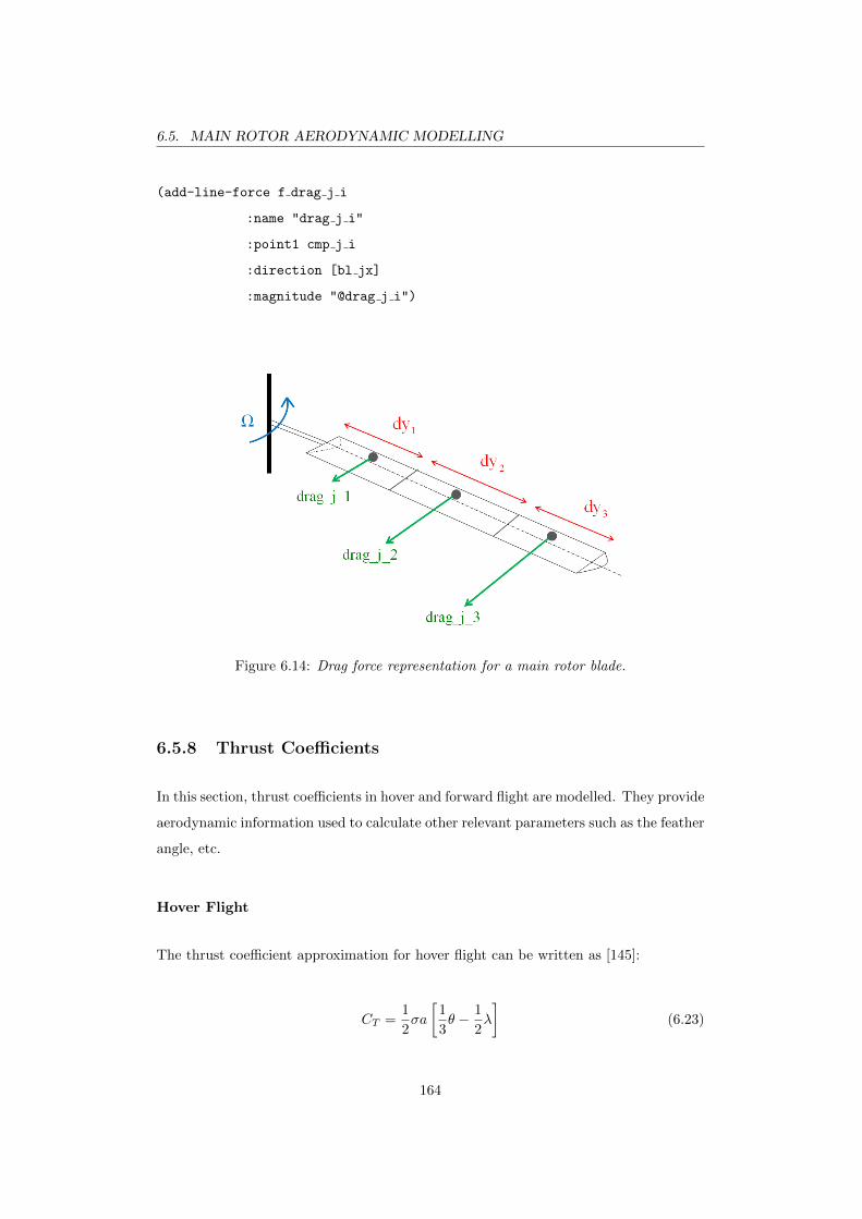
6.5. MAIN ROTOR AERODYNAMIC MODELLING
(add-line-force f drag j i
:name "drag j i"
:point1 cmp j i
:direction [bl jx]
:magnitude "@drag j i")
Figure 6.14: Drag force representation for a main rotor blade.
6.5.8 Thrust Coefficients
In this section, thrust coefficients in hover and forward flight are modelled. They provide
aerodynamic information used to calculate other relevant parameters such as the feather
angle, etc.
Hover Flight
The thrust coefficient approximation for hover flight can be written as [145]:
CT =1
2σa
[1
3θ − 1
2λ
](6.23)
164
6.5. MAIN ROTOR AERODYNAMIC MODELLING
θ is the feather angle, a is the lift slope, λ = vih/ΩR, vih is the induced hover velocity,
R is the rotor radius and σ is the solidity factor which for a constant blade chord is
given by:
σ =Nc
πR(6.24)
N is the number of main rotor blades and c is the blade chord.
The solidity factor, σ, is implemented in VehicleSim as a variable:
(setsym solifc "(nblades*chord)/(@pi*Rt)")
nblades is the number of blades and the rest of variables have been defined before.
The thrust coefficient is now modelled as:
(setsym Ct j "cte*@solifc*2*@pi*(((1/3)*rq(pj j))-(cte*(@vih/
(omega*Rt34)))))")
Rt34 is the rotor radius calculated as 0.75 ·Rt i.e., at three quarters of the radius value.
This distance is usually used as reference, because modern blades have a negative degree
of twist, decreasing the feather angle towards the tip [145]. The rest of variables have
been defined previously.
Forward Flight Conditions
The thrust coefficient in forward flight is given by [145]:
CT =1
2σa
[1
3θ0
(1 +
3µ2
2
)− 1
2λ
](6.25)
This is the simplest expression for the lift coefficient of a rotor in forward level flight.
This equation is valid if the value of θ is taken to be that at three quarters of the radius.
The variables involved in this equation are calculated at three quarters of the radius.
By using blade element theory in forward flight, the variables involved in the thrust
coefficient can be modelled.
Taking into account equations (6.7), (6.8) and (6.10) at 0.75Rt, the inflow factor can
now be calculated at three quarters of the radius:
165

6.5. MAIN ROTOR AERODYNAMIC MODELLING
(setsym lambda34 "mu*sin(gamma)+@ld ifw34")
where the variable @ld ifw34 is given as:
(setsym ld ifw34 "(Kfw*@vih)/(omega*Rt34)")
UT and UP are implemented as the variables @ut34 and @up34 respectively:
(setsym ut34 "(omega*Rt34)+(omega*Rt34*mu*sin(@wrotor*t))")
(setsym up34 "@wrotor*Rt34*@lambda34+(@wrotor*Rt34*mu*cos(@wrotor*t)*
rq(fj j))+(Rt34*dxdt(rq(fj j)))")
The angle of attack is given by (6.11) and is modelled as the variable @alp34:
(setsym alp34 "rq(pj j)-(@up34/@ut34)")
Therefore, taking into account equation (6.25), the thrust coefficient in forward flight
is:
(setsym Ctfw "cte*@solifc*2*@pi*((1/3)*fo*(1+((3*mu**2)/2))-
(cte*@lambda34))")
fo is the collective feather angle and mu is the advance ratio. The rest of variables have
already been defined.
6.5.9 Climb Angle
Blade element theory can be used to estimate the collective feather increase required
for climb [140].
∆θ =3
2
V + v − vhΩR
(6.26)
V is the climb speed, v is the induced climb speed and vh in the hover speed.
The climb angle is modelled in VehicleSim as:
(setsym dthetacl "(3/2)*((@vc+@viclmb-@vih)/(omega*Rt))")
166
6.6. TAIL ROTOR AERODYNAMIC MODELLING
6.6 Tail Rotor Aerodynamic Modelling
6.6.1 Blade Angle of Incidence for Hover, Climb, Descent and
Forward Flight
The aerodynamic forces acting on a blade segment at a given azimuth position on the
tail rotor disc are calculated using blade element theory. The local angle of attack α,
depends on the instantaneous conditions of blade profiles’ airflow along the rotor radius
[74]:
α = θ − arctan(VoutVin
)(6.27)
θ is the tail rotor blade feather angle, Vout and Vin are the components of the blade
profile airflow: out of plane and in plane of tail rotor disc, respectively.
Hover Flight Conditions
The induced velocity on the tail rotor in hovering flight is given by [73]:
Vi0 =
√F
2ρS(6.28)
F is the tail rotor lift force in hovering, S is the tail rotor disc area and ρ is the air
density in the flight level.
The angle of incidence is given by:
α = θ − arctan(Vi0Ωr
)(6.29)
θ is the blade feather angle, Ω is the tail rotor angular speed and r is the corresponding
length on the tail rotor where the aerodynamic load is applied.
Taking into account the previous equations, the angle of incidence on the tail for hover
conditions is implemented. First, the induced velocity in hovering flight is modelled as
in equation (6.28):
(setsym vih tl "sqrt(((mf+mbl1+mbl2+mbl3+mbl4+mbl tl1+mbl tl2)*g)/
(2*@ro air*@pi*R tl**2)))")
167
6.6. TAIL ROTOR AERODYNAMIC MODELLING
where R tl is the tail rotor radius, the rest of variables have been defined before.
Then, using equation (6.29), the angle of incidence is implemented as:
(setsym alphatl p i "rq(pj tl p)-arctg(@vih tl/((k rt tl*omega)*zt i))")
where p = 1, 2 and i = 1, .., 3, rq(pj tl p) is the blade feather angle and zt i is the
distance along the Z axis of the tail rotor blade.
Climb Flight Conditions
Similarly, by using blade element theory, the angle of incidence in climb can be modelled.
In this case, the velocity in climb flight is:
(setsym vc tl "cteclimb*(Kclimb*@vih tl)")
where cteclimb is a boolean variable, its function was explained previously. Kclimb
is a constant value that will be defined by the climb velocity. Finally, @vih tl is the
induced hover velocity mentioned before.
The angle of incidence in climb conditions is modelled in VehicleSim as:
(setsym alptlc p i "rq(pj tl j)-arctg(@vc tl/((k rt tl*omega)*zt i))")
Descent Flight Conditions
The velocity in descent flight can be implemented as:
(setsym vides tl "ctevid*(kdes*@vih tl)")
where ctevid is a boolean variable. kdes is a constant value that will be defined by the
descent velocity. Finally, @vih tl is the induced hover velocity was explained previously.
The angle of incidence in descent flight is given by:
(setsym alptld p i "rq(pj tl j)-arctg(@vides tl/((k rt tl*omega)*zt i))")
168
6.6. TAIL ROTOR AERODYNAMIC MODELLING
Forward Flight Conditions
In forward flight, the velocity components on the blade element are periodic, vary with
the azimuth position of the blade, ψ. Taking into account [73], the air speed’s tangential
component UT , is written as:
UT = Ωr + V0sinψ (6.30)
r is the length of the tail rotor blade where the aerodynamic force is considered, V0
is the helicopter velocity with respect to the air. Considering [73], the air speed’s
perpendicular component UP is given by:
UP = (r − e) β + (V0cosψ)β + Vi (6.31)
Vi is the induced velocity in forward flight.
The angle of incidence can be obtained as:
α = θ − UPUT
(6.32)
As in equation (6.30), UT is modelled as:
(setsym ut tl p i "((k rt tl*omega)*zt i)+(omega*Rt*mu*sin((k rt tl*
@wrotor)*t))")
and UP is:
(setsym up tl p i "@vifw+(@wrotor*Rt*mu*cos((k rt tl*@wrotor)*t)*
rq(fj tl p))+(zt i*dxdt(rq(fj tl p)))")
Finally, the angle of incidence is modelled as:
(setsym alptlfw p i "rq(pj tl p)-(@up tl p i/@ut tl i)")
6.6.2 Tail Rotor Lift Force
The lift coefficient in hover, climb, descent and forward flight can be written respectively
as:
169

6.6. TAIL ROTOR AERODYNAMIC MODELLING
(setsym cltl p i "2*@pi*@alphatl p i")
(setsym cltlc p i "2*@pi*@alptlc p i")
(setsym cltld p i "2*@pi*@alptld p i")
(setsym cltlfw p i "2*@pi*@alptlfw p i")
The resultant lift force per unit span on the tail blade element in forward flight is [144]:
L =1
2U2T cCl
(θ − UP
UT
)dr (6.33)
being the expressions for hover, climb and descent analogous to the expression used in
the main rotor. As a result, the lift force on the tail rotor can be modelled as:
(setsym lf tl p i "cte*@ro air*((ctecl*((k rt tl*@wrotor*zt i)**2)*
@cltlc p i)+(ctvids*((k rt tl*@wrotor*zt i)**2)*@cltld p i)+
(ctehv*((k rt tl*@wrotor*zt i)**2)*@cltl p i)+
(ctefw*(@ut tl p**2)*@cltlfw p i))*chordt*dz i")
where chordt is the chord of the tail rotor blade and zt i are the different points on
the tail rotor blades where the lift forces are applied to. Finally, dz i are the differential
length intervals in which the differential lift forces are divided.
Various points in the helicopter’s nominal configuration are defined to allow the mod-
elling of the lift force, these are defined on the body n:
(add-point cmptl p i :body n :coordinates ("-xt ± xt i" -yt "-ht ± zt i"))
where p = 1, 2 (tail rotor number of blades) and i = 1, .., 3 (points on the tail rotor
blades where the aerodynamic load are applied).
The points cmt p i define the centre of pressure which are points on the tail rotor
blades.
(add-point cmt p i :body bl tl p :coordinates cmptl p i)
The command add-line-force introduces the lift forces in the model:
(add-line-force f lift tl p i
:name "lift tl p i"
170
6.6. TAIL ROTOR AERODYNAMIC MODELLING
:point1 cmt p i
:direction [bl tl py]
:magnitude "@lf tl p i")
6.6.3 Tail Rotor Thrust Coefficient
The tail rotor thrust coefficient is calculated once some previous coefficients are intro-
duced and calculated:
s =bc
πR(6.34)
being s the solidity, b the tail rotor number of blade, c is the chord of the tail rotor
blade and R is the tail rotor radius. In addition to this, the thrust coefficient can be
written as:
tcD =a
4
[2
3θ0
1− µ2 + 9µ4/4
1 + 3µ2/2+ λD
1− µ2/2
1 + 3µ2/2
](6.35)
The H-force coefficient can also be written as:
hcD =1
4µδ +
aµλD4
[(θ0/3)
(1− 9µ2
)1 + 3µ2/2
+λD
1 + 3µ2/2
](6.36)
The torque coefficient is:
qc =δ(1 + 3µ2
)8
− λDtcD − µhcD (6.37)
So, the rotor torque is calculated as:
Q = qcρsAΩ2R3 (6.38)
The tail rotor thrust is [141]:
Tt =Q
ltR(6.39)
where ltR is the distance from the tail rotor to the helicopter’s centre of gravity.
Finally, the thrust coefficient based on disc area is [72]:
Ct =T
πR2ρ (ΩR)2 (6.40)
171
6.7. FLIGHT CONTROL
Taking into account the previous expressions, the tail rotor thrust coefficient can be
modelled in VehicleSim as:
(setsym lambda D "mu*sin(gamma)-@lbda ifw")
(setsym solif tl "(nblades tl*chordt)/(@pi*R tl)")
(setsym tcd "((2*@pi)/4)*((2/3)*fo*((1-(mu**2)+(9*mu**4))/4)/
(1+(3*(mu**2))/2))+@lambda D*((1-((mu**2)/2))/(1+((3*(mu**2))/2))))")
mu is the advance ratio.
(setsym hcd "((1/4)*mu*@cd 34fw+((2*@pi*@lambda D)/4)*(((fo/3)*
(1-((9*(mu**2))/2))/(1+((3*(mu**2))/2))+(@lambda D/(1+((3*mu**2)/2))))")
@cd 34fw is the drag coefficient calculated at 0.75 ∗Rtl and it is given by:
(setsym cd 34fw "delta0+delta1*@alp34+delta2*@alp34**2")
and @alp34 is the tail rotor blade’s angle of incidence, and it is implemented as:
(setsym alp34 "rq(pj j)-atan(@up34/@ut34)")
(setsym qc "(@cd 34fw*(1+(3*(mu**2)))/8)-(@lambda D*@tcd)-(mu*@hcd)")
(setsym Q "@qc*@ro air*@solifc*(@pi*(Rt**2))*(@wrotor**2)*(Rt**3)")
(setsym Tt "@Q/(xt+xfs)")
xt+xfs is the tail rotor’s distance from the helicopter’s centre of mass:
(setsym Cttail "@Tt/((@pi*(R tl**2))*@ro air*((k rt tl*omega)*R tl)**2)")
@Cttail is the VehicleSim variable implemented to model the tail rotor thrust coeffi-
cient.
6.7 Flight Control
As a consequence of the aerodynamic load action on the helicopter, various controllers
on the rotational and the translational degrees of freedom must be implemented. So
that at all the times a stable trajectory can be achieved. Aerodynamic forces and loads
172
6.7. FLIGHT CONTROL
do have an impact on the vehicle’s trajectory and therefore there exist a clear need for
paying special attention to the flight control aspects. This is a fundamental step in the
aerodynamic model here presented.
6.7.1 Longitudinal Position Control
In order to control the helicopter’s position and displacement on the X axis, some
means of control need to be implemented. The longitudinal position of the helicopter
is implemented by first defining the following variables:
(setsym x long "dir(cross([fuselagey],[nz]))")
(setsym xheli "dot(pos(fuselage0,n0),@x long)")
The first line, defines the longitudinal direction of the fuselage. The second line finds
the fuselage longitudinal position in the direction of @xlong.
The helicopter speed in forward flight is implemented as:
(setsym vheli "(mu*Rt*@wrotor)/cos((ktray1*gamma)+(ktray2*@phi fusey))")
where mu is the advance ratio and the rest of variables have been defined before.
(setsym xref "x ref+@vheli*t")
The variable xref is added to represent the longitudinal trajectory prescription for
the fuselage’s longitudinal position. It provides the reference value for the longitudinal
position; it allows to describe the trajectory in the space. gamma is the flight path angle
and its numerical value is defined at the beginning of the program.
(setsym xerror "@xref-@xheli")
(add-state-variable xfutq xfutqp "F")
(set-aux-state-deriv xfutqp "kix*@xerror")
The command add-state-variable introduces a state variable for the force expressions
used to control the helicopter’s longitudinal position. The integral part of the force is
defined by the command set-aux-state-deriv and it uses the value of the variable
@xerror defined as the difference between the actual and prescribed longitudinal posi-
tions.
173
6.7. FLIGHT CONTROL
(add-line-force xcon
:name "xctrl"
:direction [fuselagex]
:point1 fuselage0
:point2 n0
:magnitude "xfutq+kpx*(@xerror)+kdx*dxdt(@xerror)")
The force is applied between the fuselage (centre of the fuselage fuselage0) and the
inertial frame. The controller uses the variable @xerror as the input variable and the
output is the force applied to the fuselage so a desired longitudinal position control is
achieved. The parameters kix, kpx and kdx are the gains of the controller that is of
PID type.
The lateral position control is modelled similarly to the controller explained in Chapter
5 and therefore it is not included in this report.
6.7.2 Vertical Position Control
In order to control the position of the helicopter on the Z axis, a new controller needs
to be implemented. In a similar way to the longitudinal position control defined before,
the vertical position of the helicopter is calculated after defining two necessary variables:
(setsym z long "dir(cross([fuselagex],[ny]))")
(setsym hheli "dot(pos(fuselage0,n0),@z long)")
The first line, defines the vertical direction of the fuselage, @z long. The last one finds
the fuselage’s vertical position, @hheli, this is, the height.
The helicopter’s velocities in climb and descent fight are modelled as:
(setsym vcc "(ctecl*@vc)+(ctvids*@vdes)")
where ctecl, ctvids are boolean variables defining the helicopter’s ascending @vc or
descending @vdes velocities, respectively.
(setsym href "-height-@vcc*t")
The variable @href is added as the helicopter’s vertical trajectory prescribed for the
vertical position.
174
6.7. FLIGHT CONTROL
(setsym herror "@href-@hheli")
(add-state-variable hfu tq hfu tqp "F")
(set-aux-state-deriv hfu tqp "kih*@herror")
The command add-state-variable introduces a state variable, for the force expression
is used to control the vertical position. The integral part of the force is defined by the
set-aux-state-deriv command and uses the value of the @herror defined before.
(add-line-force hcon
:name "hctrl"
:direction -[fuselagez]
:point1 fuselage0
:point2 n0
:magnitude "hfu tq+kph*(@herror)+kdh*dxdt(@herror)")
The force is applied between the fuselage and the inertia frame. The controller uses
the variable @herror as the input variable and the output is the force applied to the
fuselage so the desired vertical position is achieved. The parameters kih, kph and kdh
are the controller’s gains.
Fuselage’s Yaw Control
In order to control the helicopter’s yaw, a new controller needs to be added. The yaw
angle is obtained as the first rotational coordinate of the fuselage:
(setsym phi fusez "rq(fuselage,1)")
The sideslip angle in forward flight is [72]:
ηt = tan−1
(tanη − rlt
V cosη
)(6.41)
where η is the sideslip angle (angle between plane of symmetry and flight path). V is
forward velocity, r is the yaw speed and lt is the distance of the tail rotor from the
centre of the fuselage (see Figure 6.15).
The variable @phi refz is defined as the fuselage’s yaw reference value. This is an equa-
tion that allows to describe a yaw helicopter trajectory in the space. It is implemented
in VehicleSim as:
175
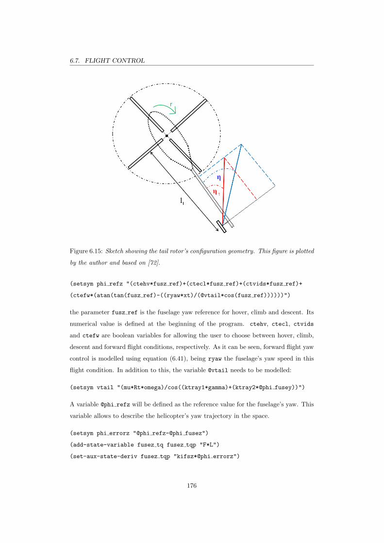
6.7. FLIGHT CONTROL
Figure 6.15: Sketch showing the tail rotor’s configuration geometry. This figure is plotted
by the author and based on [72].
(setsym phi refz "(ctehv*fusz ref)+(ctecl*fusz ref)+(ctvids*fusz ref)+
(ctefw*(atan(tan(fusz ref)-((ryaw*xt)/(@vtail*cos(fusz ref))))))")
the parameter fusz ref is the fuselage yaw reference for hover, climb and descent. Its
numerical value is defined at the beginning of the program. ctehv, ctecl, ctvids
and ctefw are boolean variables for allowing the user to choose between hover, climb,
descent and forward flight conditions, respectively. As it can be seen, forward flight yaw
control is modelled using equation (6.41), being ryaw the fuselage’s yaw speed in this
flight condition. In addition to this, the variable @vtail needs to be modelled:
(setsym vtail "(mu*Rt*omega)/cos((ktray1*gamma)+(ktray2*@phi fusey))")
A variable @phi refz will be defined as the reference value for the fuselage’s yaw. This
variable allows to describe the helicopter’s yaw trajectory in the space.
(setsym phi errorz "@phi refz-@phi fusez")
(add-state-variable fusez tq fusez tqp "F*L")
(set-aux-state-deriv fusez tqp "kifsz*@phi errorz")
176
6.7. FLIGHT CONTROL
The add-state-variable command introduces a state variable for the torque expres-
sion that it is used to control the helicopter’s yaw. The integral part of the torque is de-
fined with the set-aux-state-deriv command and uses the value of the @phi errorz
defined above. The variable @phi errorz is the difference between the fuselage’s actual
and desired yaw position.
(add-moment fsz phi
:name "phi ctrlz"
:direction -[fuselagez]
:body1 fuselage
:body2 n
:magnitude "fusez tq+kpfsz*(@phi errorz)+kdfsz*dxdt(@phi errorz)")
The moment is applied between the fuselage and the inertia frame. The controller uses
the variable @phierrorz as the input variable, and the output is the moment applied
to the fuselage, so satisfactory yaw control is achieved. The parameters kifsz, kpfsz
and kdfsz are the controller’s gains.
6.7.3 Tail Rotor Flap Control
In order to control the tail rotor blade’s flap under the effect of the delta three angle,
some previous considerations should be considered.
The coning angle is reduced for a given collective feather angle as indicated in [144]:
a0 =Γ(θ0 − 4
3λ)
8 + Γtanδ3(6.42)
In addition to this, the flap coefficients a1 and b1 can be written as indicated in [147]:
a1 =q
Ω
(16Γ −K
)1 +K2
(6.43)
b1 = −q(1 +K 16
Γ
)Ω (1 +K2)
(6.44)
where K = tan δ3, q is the component of the rotor axis tilt rate in the feather plane of
the rotor, and Γ is given by:
177
6.8. CHAPTER SUMMARY
Γ =cρaR4
If(6.45)
being the mass (inertia) constant of the blade to zero flap hinge offset.
Taking into account the previous considerations about the delta three angle, the tail
rotor blade’s flap motion can be modelled now:
(setsym gamma tl "(@ro air*(2*@pi)*chordt**(R tl**4))/Iblx tl")
where Iblx tl is the moment of inertia about the flap axis.
The flap harmonics can be modelled using the previous equations:
(setsym a0 "(@gamma tl*(fo tl-((4/3)*@lbda ifw)))/(8+@gamma tl*
tan(delta3 tl))")
(setsym a1 "(alpha tp/(k rt tl*omega))*(((16/@gamma tl)-tan(delta3 tl))/
(1+((tan(delta3 tl))**2)))")
(setsym b1 "-(alpha tp*(1+(tan(delta3 tl)*(16/@gamma tl)))/
((k rt tl*omega)*(1+((tan(delta3 tl))**2))))")
fo tl is the tail rotor collective feather and alpha tp is the tail plane incidence setting
its numerical values at the beginning of the program.
6.8 Chapter Summary
This chapter provides a description of the modelling process when there exist external
forces on the helicopter model described in Chapter 5. The first step taken, was to
consider the aerodynamic environment. In here, the forces acting on a helicopter were
described as well as the rotor blades angles i.e., angle of incidence and angle of attack.
In addition to this, blade element theory in hover, axial and forward flight was applied.
Gravity and its effect was the first external force to be included in the model. Im-
plementation of the ground on the fuselage in absence of aerodynamic loads has been
considered. Once the gravity force was added to the existing model, the main rotor
tilt was modelled as well. A main rotor local axis was defined in terms of the inertial
178
6.8. CHAPTER SUMMARY
reference axes with respect to the fuselage.
Other external perturbation was as well modelled in absence of aerodynamic load; a
change on the main rotor’s angular speed following some specific demand. As a result,
three frequencies were defined and an acceleration was also provided. A PID controller
was implemented in order to change the main rotor angular speed.
The aerodynamic modelling process has been described in detail, first on the main rotor
and after that on the tail rotor. The air density has an influence on the aerodynamic
equations, it was modelled by taking into account the entire height range reached by
helicopters during flight. The induced hover speed was described and implemented, as a
consequence of this, climb, descent and forward speeds were also obtained. Additionally,
induced climb, descent and forward speed were provided using the induced hover speed.
Once the speeds and the induced speeds were modelled, the blade’s angle of incidence
was modelled in hover, climb, descent and forward flight separately. This allowed to
obtain the lift and the drag forces on the main rotor blades. The thrust coefficients
in hover and forward flight were also included in the model. On the other hand, the
collective feather increase required in climb was calculated.
The tail rotor aerodynamic model was implemented too, the blade’s incidence angles
for hover, climb, descent and forward flight were modelled. Given that, the lift force on
the tail could then be modelled. The tail rotor thrust coefficient was analyzed and also
included in the model.
The flight control methodology was described, this a fundamental task in order to
achieve prescribed trajectories. Longitudinal, vertical positions control and fuselage
yaw control were implemented using PID controllers. Finally, the tail rotor flap control
was modelled.
As it can be seen, this chapter contains a comprensive and details model of the aerody-
namical load and its effects on the helicopter system.
For the modelling process, previous existing theoretical approaches have been considered
and adequately referenced along the chapter.
179

Part III
Results
180
Chapter 7
Sikorsky Model in Absence of
External Perturbations
This chapter is aimed at furthering the understanding of the dynamic behaviour of a
helicopter in vacuum and without gravity. The effect of each property is individually
analyzed by assuming that the nominal helicopter configuration is the one described in
Chapter 5. The analysis is done purely through simulations and validated by comparing
the results with existing theory. The equations of motion are obtained for flap, lag, flap-
lag coupled and feather dynamics. A blade dynamic analysis is carried out, the fuselage
and its interaction with the main rotor as well as the tail rotor are also studied. After
that, main and tail rotors’ angular speeds are introduced/implemented by using the
torques on the rotors. The six degrees of freedom of the helicopter and their stability
are studied. Finally, the vibrations appearing on the fuselage are studied; structural
unbalances are generated on the main and tail rotors respectively for this purpose.
7.1 VehicleSim Equations of Motion
Once the model has been built, the symbolic multibody software VehicleSim derives the
linear and nonlinear equations of motion for the dynamics involved in the system as
well as the time series representing the nonlinear behaviour. In order to validate the
model, the results here presented will be compared to those predicted by the theory and
181
7.1. VEHICLESIM EQUATIONS OF MOTION
experimental tests. Initially, the results for the case of uncoupled flap and lag degrees
of freedom are presented. After that, both of them will be studied simultaneously and
their coupling will be analysed and compared to existing theoretical knowledge. Finally,
feather equations are also provided and analysed. It is convenient to remind at this point
that the case under study is for rigid blades, being flexibility and torsion two properties
not considered at present in this work.
7.1.1 Flap Dynamical Equations
Flap is the first degree of freedom of the blade under consideration. In order to model
the flap mode, a spring is included in the flap hinge, it creates a restoring moment
on the blade. If the spring stiffness is zero, the flap natural frequency is equal to the
angular frequency of the main rotor. The flap offset is the distance existing between the
rotor hub and the flap hinge. It is provided as a percentage e% of the radius R of the
blade. Once the blade (flap) model is built, simulations are carried out with VehicleSim
in order to generate the linear and nonlinear equations. This same program script can
then be used to study the behaviour of the system under several conditions as external
forces.
One of the most comprehensive surveys on rotor dynamics is proposed by [141], here
the flap motion is represented by a second order differential equation of the form:
Bβ + Ω2(Bcosβ +MbexgR
2)sinβ = MA (7.1)
B is the moment of the inertia around the flap axis, MA is the aerodynamic moment
and Mb is the blade mass. In this reference, the position vector of the blade c.g (centre
of gravity) is rg = xgR. In our system, the c.g of the blade is considered to lie on the
longitudinal axis, so it can be written as rg = yg. The equations are obtained by using
the term eR instead of eR2. Approximations for small angles, cosβ ∼= 1 and sinβ ∼= β
can be applied to equation (7.1). Thus, it can be written as:
Bβ + Ω2(B +MbexgR
2)β = MA (7.2)
182
7.1. VEHICLESIM EQUATIONS OF MOTION
VehicleSim Linear Flap Equation
The flap dynamics linear equation is obtained by using the appropriate Lisp code com-
mands in VehicleSim, the application of such a linearization provides the equation:
β(Iblx +mbly
2bl
)= −mblΩ
2ybl (eR+ ybl)β − Ω2 (Iblz − Ibly)β (7.3)
A simple comparison between equations (7.2) and (7.3) can be done. Similarities be-
tween both equations are found. The moment of inertia around the blade’s flap axis, is
given by Iblx + mbly2bl. If a plane figure is considered, then, Iz = Ix + Iy and equation
(7.3) can be now written as:
β(Iblx +mbly
2bl
)= −Ω2
(Iblx +mbly
2bl +mbleRybl
)β (7.4)
It is clear to see that both equations (7.2) and (7.4) are similar except for the presence
of aerodynamical moments as in this section they are not considered.
When the model has a spring fitted in the flap hinge it generates a restoring moment
on the blade. VehicleSim equation obtained in this case yield the following expression
which contains the restoring moment:
β(Iblx +mbly
2bl
)= −mblΩ
2ybl (eR+ ybl)β − Ω2 (Iblz − Ibly)β − kfjβ (7.5)
being kfj the spring stiffness coefficient.
From equation (7.5), the blade’s flap frequency can be obtained as:
ν =
√Ω2 [eRmblybl +mbly2
bl + (Iblz − Ibly)] + kfj(Iblx +mbly2
bl)(7.6)
which is ν = 48.856 rad/s if the parameters involved in this expression, Ω, eR, mbl, ybl
amongst others, are substituted by the corresponding numerical values of a real Sikorsky
model.
If a simulation is carried out for a blade with pure flap degree of freedom for 50 s with an
initial flap angle, β0 = 0.0175 rad, the VehicleSim obtained flap mode frequency is 7.78
Hz or (48.88 rad/s), this value was calculated using a FFT (Fast Fourier Transform)
Matlab algorithm. This frequency is near to the angular frequency of the rotor, as it
was expected following theoretical predictions [148]. The value of the frequency is now
183

7.1. VEHICLESIM EQUATIONS OF MOTION
slightly higher as the offset and the spring stiffness increase it. These effects will be
analysed in the next sections.
VehicleSim NonLinear Flap Equation
In the nonlinear case, VehicleSim can also derive the equations of motion. The nonlinear
equation for the flap dynamics is generated by stating the corresponding Lisp code
commands. Two cases are presented in here, with and without spring in the flap hinge.
• NonLinear Flap Equation without Spring Stiffness
β(Iblx +mbly
2bl
)= −eRmblyblΩ
2sinβ −mbly2blΩ
2cosβsinβ − (Iblz − Ibly) Ω2cosβsinβ
(7.7)
If a comparison between equations (7.1) and (7.7) is made, similarities between them are
observed. Taking into account the previous considerations about the centre of gravity,
plane blade amongst others, equation (7.7) now is:
β(Iblx +mbly
2bl
)= −Ω2
((Iblx +mbly
2bl
)cosβ +mbleRybl
)sinβ (7.8)
It is seen that equation (7.1) and equation (7.8) are equal if MA = 0.
• NonLinear Flap Equation with Spring Stiffness
VehicleSim provides the following equation that contains the term corresponding to the
spring force.
β(Iblx +mbly
2bl
)= −eRmblyblΩ
2sinβ −mbly2blΩ
2cosβsinβ − (Iblz − Ibly) Ω2cosβsinβ
−kfjβ(7.9)
The nonlinear equation (7.9) has been validated by using a Lagrangian approach and
this derivation is included in Appendix A.
7.1.2 Lag Dynamical Equations
In this section, the author analyzes pure lag motion and validates the obtained results.
This is, the lag equations of motion in the absence of a flap hinge are obtained by using
184
7.1. VEHICLESIM EQUATIONS OF MOTION
VehicleSim Lisp and compared to those available in the literature. In order to validate
the equations obtained by VehicleSim, the following accepted expression for pure lag
motion is taken into consideration [141]:
Cξ +MbexgΩ2R2sinξ = N (7.10)
where C is the moment of the inertia about the lag axis, N is the aerodynamic lag
moment and Mb is the blade mass. Now, if small angles approximation is taken, then
equation (7.10) can be simplified to:
ξ + Ω2εξ = N/C (7.11)
where ε is MbexgR2/C and eR is the corresponding lag hinge offset distance.
VehicleSim Linear Lag Equation
The linear equation for the lag is generated by using corresponding commands in Lisp
code. The application yields the following expression:
ξ(Iblz +mbly
2bl
)+ eRmblΩ
2yblξ = 0 (7.12)
Now, equation (7.11) is compared to equation (7.12). The previous considerations about
the c.g and the null value for the aerodynamic lag moment and the moment of the inertia
around the lag axis (C) being equal to Iblz +mbly2bl need to be taken into account. It is
clear to see that equations (7.11) and (7.12) are equivalent.
By now, equation (7.12) does not have any spring stiffness or damping coefficient in-
cluded. In the total moment calculation, a spring is included in order to get the equi-
librium moment about the lag hinge [140]. Moreover, a damper is also used in the lag
hinge, because when the aerodynamic forces are considered, their damping is usually
not enough to allow the lag motion and the blade can be under the effect of unwanted
stress forces [144].
• Linear Lag Equation with Spring Stiffness and Damping Coefficient
185
7.1. VEHICLESIM EQUATIONS OF MOTION
If these are included in the system, the VehicleSim equation of motion is as follows:
ξ(Iblz +mbly
2bl
)= −eRmblΩ
2yblξ − dlj ξ − kljξ (7.13)
From the above expression, the blade’s lag mode frequency is obtained:
ν =
√eRmblyblΩ2 + klj
(Iblz +mbly2bl)
(7.14)
By substituting the parameters’ values involved in equation (7.14) from the Sikorsky
model, it is shown that the lag mode frequency is 5.63 Hz or (35.38 rad/s).
VehicleSim NonLinear Lag Equation
For the nonlinear lag case, the equations can be obtained by using VehicleSim:
• NonLinear Lag Equation without Spring Stiffness and without Damping Coeffi-
cient
ξ(Iblz +mbly
2bl
)+ eRmblΩ
2yblsinξ = 0 (7.15)
A comparison between equation (7.10) (theoretical prediction) and equation (7.15) is
performed. Taking into account the previous considerations for the c.g, the aerodynamic
lag moment and the moment of the inertia around the lag axis, it is seen how this two
expressions are equivalent. Equation (7.15) is validated in this way.
• NonLinear Lag Equation with Spring Stiffness and with Damping Coefficient
If now both a spring and a damper are included in the model, the VehicleSim nonlinear
equation of motion is given by:
ξ(Iblz +mbly
2bl
)= −eRmblΩ
2yblsinξ − dlj ξ − kljξ (7.16)
where dlj and klj are the damping coefficient and spring stiffness respectively.
The nonlinear equation (7.16) can be validated by using the Lagrangian Mechanic ap-
proach (see Appendix B for the mathematical derivation).
186

7.1. VEHICLESIM EQUATIONS OF MOTION
7.1.3 Feather Equations of Motion
The feather is the third degree of freedom allowed on the blade’s motion. The feather
motion can be described by the following equation [141]:
Aθ +AΩ2sinθcosθ = L (7.17)
where θ is the feather angle, A is the moment of inertia on the longitudinal blade axis
and L is the moment on the feather axis. In many cases, feather motion takes place
only for small angles, so this can be simplified as:
θ + Ω2θ = L/A (7.18)
VehicleSim Linear Feather Equation
Using VehicleSim to obtain the feather motion linear equation yields:
θ(Ibly +mblx
2bl
)=((Iblx − Iblz)−mblx
2bl
)Ω2θ (7.19)
Analogies between the equations (7.18) and (7.19) can be found. Taking into account
that for a plane figure, the ratio Iz = Ix + Iy is satisfied and that the moment about
the feather axis is zero, equation (7.19) can be written as:
θ(Ibly +mblx
2bl
)+(Ibly +mblx
2bl
)Ω2θ = 0 (7.20)
Equations (7.18) and (7.20) are similar with A = (Ibly +mblx2bl).
VehicleSim NonLinear Feather Equation
The nonlinear equation for feather motion can be obtained with VehicleSim. This
equation matches that proposed by [141] (see equation (7.17)):
θ(Ibly +mblx
2bl
)= −mblΩ
2x2blcosθsinθ + Ω2 (Iblx − Iblz) cosθsinθ (7.21)
Grouping terms and taking into account Ibly = Iblx− Iblz, the above equation becomes:(Ibly +mblx
2bl
)θ +
(Ibly +mblx
2bl
)Ω2cosθsinθ = 0 (7.22)
Equations (7.17) and (7.22) are shown to be similar, showing in this way the validity of
the blade nonlinear model under study.
187
7.1. VEHICLESIM EQUATIONS OF MOTION
7.1.4 Coupled Equations of Flap and Lag
In most cases for articulated rotors, flap and lag hinges are mounted simultaneously
on the rotor structure. These two degrees of freedom are coupled due to the existing
Coriolis forces and the mathematical expression representing the respective motions can
become quite complex and prone to errors if they were to be hand derived. The reader
is reminded at this point that the aerodynamic forces are not considered in this work
as the author wants to focus this study in the coupled dynamics in absence of gravity
and air influence. It will be shown how the Coriolis effect introduces a coupling term
between the blade flap (out of plane motion) and the lag motion (in plane). In a rotating
frame of reference, inertial forces become relevant and cannot be neglected. On a rotor,
Coriolis forces will appear whenever there exists a radial lengthening or shortening of
the blade about the rotational axis, which is a result of the blade flap motion [98].
In a dynamic model, the forces acting on the blade for the flap motion are supported by
the inertia acceleration, its expression is given by β. The centrifugal force is supported
by the term myΩ2 and the Coriolis force appearing at the flap hinge corresponds to the
term 2mΩξ. Additionally, in the case of the lag motion, the forces are supported by the
inertia acceleration as ξ. The centrifugal force, is given by the expression myΩ2 [98].
Finally, Coriolis inertia forces are represented by the term 2BΩβsinβ, where B is the
moment of the inertia [141].
Small Order Equations for Flap/Lag Coupled Motion
The small order equations obtained in VehicleSim for the case when both flap and lag
hinges are included in the blade’s model are as follows:
Flap equation of motion:
β(Iblyξ
2 + Iblx(1− (1/2) ξ2
)2+mbly
2bl
(1− ξ2
))= −Ω2β (Iblz − Ibly) + Ωβξ
(Ibly − Iblz)−(1− (1/2) ξ2
)kfjβ −mblΩ
2yblβ (eR+ ybl)−mblΩβy2blξ
(7.23)
Lag equation of motion:
ξ(Iblz +mbly
2bl/(Iblx +mbly
2bl
)3)= IblzΩββ −mblΩ
2eRyblξ +mblΩβy2blβ
−dlj ξ − kljξ(7.24)
188
7.1. VEHICLESIM EQUATIONS OF MOTION
It is clearly seen now how these equations are coupled, as the flap degree of freedom (β)
and lag degree of freedom (ξ) depend on each other.
Non Small Order Equations for Flap/Lag Coupled Motion
Using the corresponding nonlinear set up of VehicleSim more complex expressions of
both flap and lag degrees of freedom are obtained. The modelling capabilities of Ve-
hicleSim start becoming evident now, as obtaining these equations by hand could be a
cumbersome process:
Flap equation of motion
β(Iblxcos
2ξ + Iblysin2ξ +mbly
2blcos
2ξ)− 2mblsinξy
2blcosξβξ = −kfjcosξ + Ωcos2ξsinβ
(Ibly − Iblz)(ξ + Ωcosβ
)− βcosξsinξ (Ibly − Iblz)
(ξ + Ωcosβ
)− Iblxcos2ξΩξsinβ+
Iblxcosξβsinξ(ξ + Ωcosβ
)+ Ωsinβsin2ξ (Iblx − Iblz)
(ξ + Ωcosβ
)+ βcosξsinξ
(Iblx − Iblz)(ξ + Ωcosβ
)+ IblysinξΩβcosβcosξ − Ibly ξsinξβcosξ − Ibly ξsinξΩsinβsinξ
−mblcosξybleRΩ2sinβ −mblcosβΩ2cos2ξy2blsinβ − 2mblsinβΩξy2
blcos2ξ
(7.25)
Lag equation of motion
ξ(Iblz +mbly
2bl
)+mblsinξcosξy
2blβ
2 = −kljξ − dlj ξ + IblxΩβcos2ξsinβ − (Ibly − Iblx)
sinξcosξΩ2sin2β + Ωβ(Iblz − Iblycos2ξ
)sinβ − βsinξ (Iblx − Ibly)
(βcosξ + Ωsinβsinξ
)+mblsinξcosξy
2blΩ
2sin2β −mblyblsinξeRΩ2cosβ
+mblΩsinβy2blβ −mblΩβsinβy
2blcos
2ξ +mblΩβsinβy2blsin
2ξ︸ ︷︷ ︸(∗)
(7.26)
The last three terms in equation (7.26), (∗), can be rearranged taking into account that
sinξ =√
1− cos2ξ and this yields:
mblΩsinβy2blβ −mblΩβsinβy
2blcos
2ξ +mblΩβsinβy2blsin
2ξ =
mblΩsinβy2blβ(1− cos2ξ
)+mblΩβsinβy
2blsin
2ξ(7.27)
And this is:
mblΩsinβy2blβ(1− cos2ξ
)+mblΩβsinβy
2blsin
2ξ = 2mblΩβsinβy2blsin
2ξ (7.28)
which is the corresponding Coriolis term expected to appear in the lag motion equation.
189
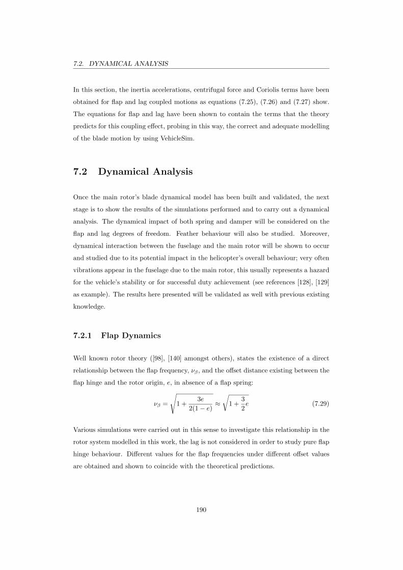
7.2. DYNAMICAL ANALYSIS
In this section, the inertia accelerations, centrifugal force and Coriolis terms have been
obtained for flap and lag coupled motions as equations (7.25), (7.26) and (7.27) show.
The equations for flap and lag have been shown to contain the terms that the theory
predicts for this coupling effect, probing in this way, the correct and adequate modelling
of the blade motion by using VehicleSim.
7.2 Dynamical Analysis
Once the main rotor’s blade dynamical model has been built and validated, the next
stage is to show the results of the simulations performed and to carry out a dynamical
analysis. The dynamical impact of both spring and damper will be considered on the
flap and lag degrees of freedom. Feather behaviour will also be studied. Moreover,
dynamical interaction between the fuselage and the main rotor will be shown to occur
and studied due to its potential impact in the helicopter’s overall behaviour; very often
vibrations appear in the fuselage due to the main rotor, this usually represents a hazard
for the vehicle’s stability or for successful duty achievement (see references [128], [129]
as example). The results here presented will be validated as well with previous existing
knowledge.
7.2.1 Flap Dynamics
Well known rotor theory ([98], [140] amongst others), states the existence of a direct
relationship between the flap frequency, νβ , and the offset distance existing between the
flap hinge and the rotor origin, e, in absence of a flap spring:
νβ =
√1 +
3e
2(1− e)≈√
1 +3
2e (7.29)
Various simulations were carried out in this sense to investigate this relationship in the
rotor system modelled in this work, the lag is not considered in order to study pure flap
hinge behaviour. Different values for the flap frequencies under different offset values
are obtained and shown to coincide with the theoretical predictions.
190
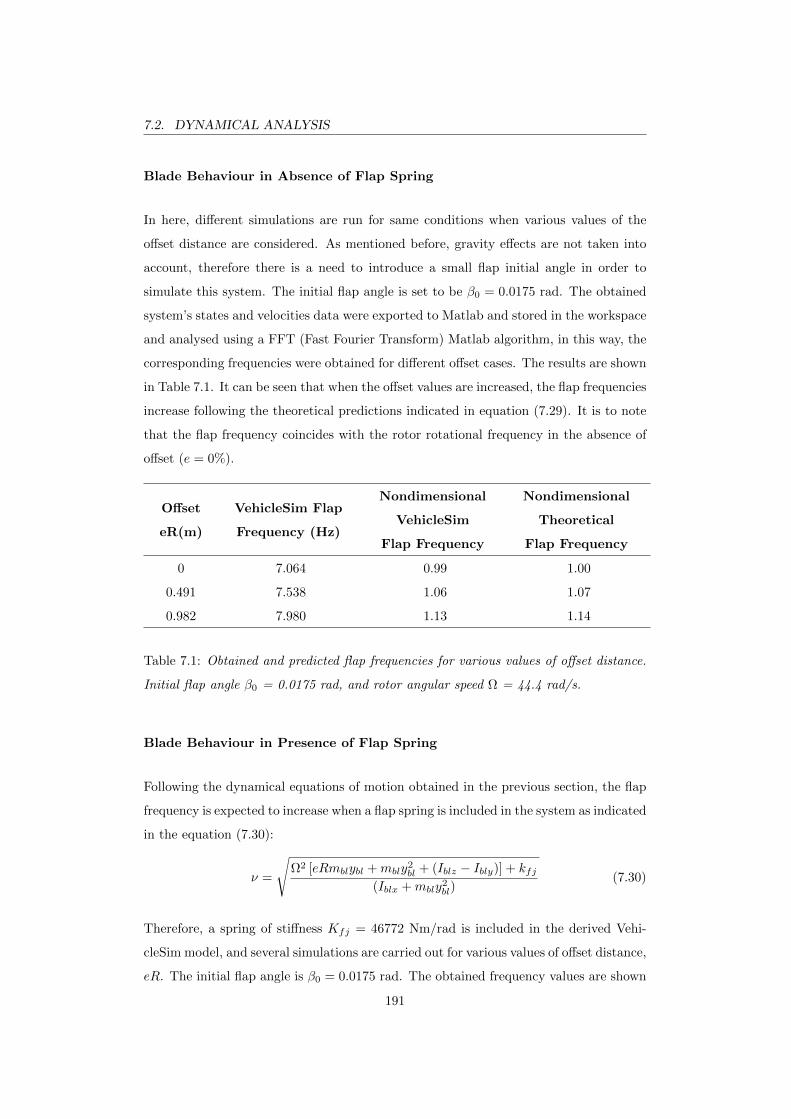
7.2. DYNAMICAL ANALYSIS
Blade Behaviour in Absence of Flap Spring
In here, different simulations are run for same conditions when various values of the
offset distance are considered. As mentioned before, gravity effects are not taken into
account, therefore there is a need to introduce a small flap initial angle in order to
simulate this system. The initial flap angle is set to be β0 = 0.0175 rad. The obtained
system’s states and velocities data were exported to Matlab and stored in the workspace
and analysed using a FFT (Fast Fourier Transform) Matlab algorithm, in this way, the
corresponding frequencies were obtained for different offset cases. The results are shown
in Table 7.1. It can be seen that when the offset values are increased, the flap frequencies
increase following the theoretical predictions indicated in equation (7.29). It is to note
that the flap frequency coincides with the rotor rotational frequency in the absence of
offset (e = 0%).
Offset
eR(m)
VehicleSim Flap
Frequency (Hz)
Nondimensional
VehicleSim
Flap Frequency
Nondimensional
Theoretical
Flap Frequency
0 7.064 0.99 1.00
0.491 7.538 1.06 1.07
0.982 7.980 1.13 1.14
Table 7.1: Obtained and predicted flap frequencies for various values of offset distance.
Initial flap angle β0 = 0.0175 rad, and rotor angular speed Ω = 44.4 rad/s.
Blade Behaviour in Presence of Flap Spring
Following the dynamical equations of motion obtained in the previous section, the flap
frequency is expected to increase when a flap spring is included in the system as indicated
in the equation (7.30):
ν =
√Ω2 [eRmblybl +mbly2
bl + (Iblz − Ibly)] + kfj(Iblx +mbly2
bl)(7.30)
Therefore, a spring of stiffness Kfj = 46772 Nm/rad is included in the derived Vehi-
cleSim model, and several simulations are carried out for various values of offset distance,
eR. The initial flap angle is β0 = 0.0175 rad. The obtained frequency values are shown
191
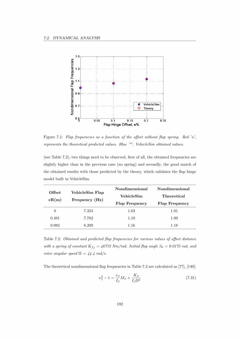
7.2. DYNAMICAL ANALYSIS
Figure 7.1: Flap frequencies as a function of the offset without flap spring. Red ’o’,
represents the theoretical predicted values. Blue ’*’, VehicleSim obtained values.
(see Table 7.2), two things need to be observed, first of all, the obtained frequencies are
slightly higher than in the previous case (no spring) and secondly, the good match of
the obtained results with those predicted by the theory, which validates the flap hinge
model built in VehicleSim.
Offset
eR(m)
VehicleSim Flap
Frequency (Hz)
Nondimensional
VehicleSim
Flap Frequency
Nondimensional
Theoretical
Flap Frequency
0 7.324 1.03 1.01
0.491 7.782 1.10 1.09
0.982 8.209 1.16 1.18
Table 7.2: Obtained and predicted flap frequencies for various values of offset distance
with a spring of constant Kfj = 46772 Nm/rad. Initial flap angle β0 = 0.0175 rad, and
rotor angular speed Ω = 44.4 rad/s.
The theoretical nondimensional flap frequencies in Table 7.2 are calculated as [77], [140]:
ν2β − 1 =
eβIβMβ +
Kβ
IβΩ2(7.31)
192
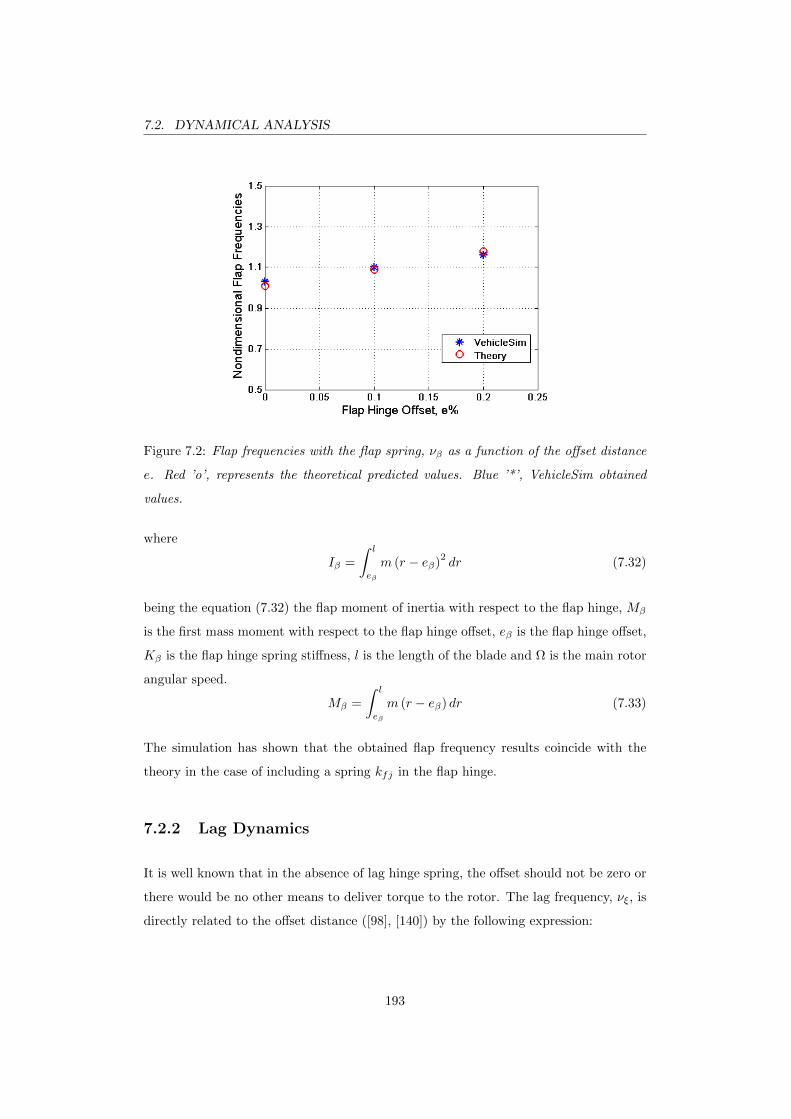
7.2. DYNAMICAL ANALYSIS
Figure 7.2: Flap frequencies with the flap spring, νβ as a function of the offset distance
e. Red ’o’, represents the theoretical predicted values. Blue ’*’, VehicleSim obtained
values.
where
Iβ =
∫ l
eβ
m (r − eβ)2dr (7.32)
being the equation (7.32) the flap moment of inertia with respect to the flap hinge, Mβ
is the first mass moment with respect to the flap hinge offset, eβ is the flap hinge offset,
Kβ is the flap hinge spring stiffness, l is the length of the blade and Ω is the main rotor
angular speed.
Mβ =
∫ l
eβ
m (r − eβ) dr (7.33)
The simulation has shown that the obtained flap frequency results coincide with the
theory in the case of including a spring kfj in the flap hinge.
7.2.2 Lag Dynamics
It is well known that in the absence of lag hinge spring, the offset should not be zero or
there would be no other means to deliver torque to the rotor. The lag frequency, νξ, is
directly related to the offset distance ([98], [140]) by the following expression:
193
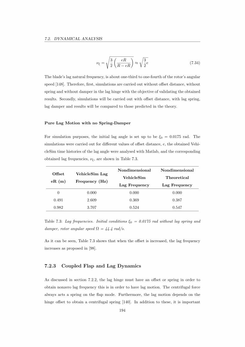
7.2. DYNAMICAL ANALYSIS
νξ =
√3
2
(eR
R− eR
)≈√
3
2e (7.34)
The blade’s lag natural frequency, is about one-third to one-fourth of the rotor’s angular
speed [148]. Therefore, first, simulations are carried out without offset distance, without
spring and without damper in the lag hinge with the objective of validating the obtained
results. Secondly, simulations will be carried out with offset distance, with lag spring,
lag damper and results will be compared to those predicted in the theory.
Pure Lag Motion with no Spring-Damper
For simulation purposes, the initial lag angle is set up to be ξ0 = 0.0175 rad. The
simulations were carried out for different values of offset distance, e, the obtained Vehi-
cleSim time histories of the lag angle were analysed with Matlab, and the corresponding
obtained lag frequencies, νξ, are shown in Table 7.3.
Offset
eR (m)
VehicleSim Lag
Frequency (Hz)
Nondimensional
VehicleSim
Lag Frequency
Nondimensional
Theoretical
Lag Frequency
0 0.000 0.000 0.000
0.491 2.609 0.369 0.387
0.982 3.707 0.524 0.547
Table 7.3: Lag frequencies. Initial conditions ξ0 = 0.0175 rad without lag spring and
damper, rotor angular speed Ω = 44.4 rad/s.
As it can be seen, Table 7.3 shows that when the offset is increased, the lag frequency
increases as proposed in [98].
7.2.3 Coupled Flap and Lag Dynamics
As discussed in section 7.2.2, the lag hinge must have an offset or spring in order to
obtain nonzero lag frequency this is in order to have lag motion. The centrifugal force
always acts a spring on the flap mode. Furthermore, the lag motion depends on the
hinge offset to obtain a centrifugal spring [140]. In addition to these, it is important
194

7.2. DYNAMICAL ANALYSIS
Figure 7.3: Lag frequencies as a function of the offset for the case of no spring, no
damper fitted in the lag hinge. Red ’o’, represents the theoretical predicted values. Blue
’*’, VehicleSim obtained values.
to note that whilst blade flap motion is essentially a resonant phenomenon; lag motion
has a natural frequency well below the rotational speed for lag hinge offset. The lag
motion natural frequency wherein spring forces are always in equilibrium with mass
forces, depends on the inertia moment and centrifugal moment, which is different from
that for flap [148]. In order to validate this, VehicleSim simulations are carried out with
a spring on the flap and lag hinges as well as a damper in the lag hinge. Similarly to the
previous sections, the simulation is carried out for an initial flap angle of β0 = 0.0175
rad, and the lag initial angle is ξ0 = 0 rad.
The theory predicts a lag frequency double those of the flap frequency [125]. Simulations
were carried out using VehicleSim for different values of the offset. The results of the
simulations are given in tables 7.4 and 7.5.
It can be seen in Table 7.5 how the ratio 2 : 1 the blade’s between lag and flap frequencies
is satisfied for the different offsets. It is clear to see how the results agree with the
theoretical predictions.
Analyzing the simulation results relating flap and lag angles, the coupling between flap
and lag arising from the nonlinear terms in equations (7.25) and (7.26) can be observed
in the decay of both signals amplitudes over time (see Figure 7.4). The simulation was
195

7.2. DYNAMICAL ANALYSIS
Offset
eR (m)
VehicleSim Flap
Frequency (Hz)
VehicleSim Lag
Frequency (Hz)β (rad/s) ξ (rad/s)
0 7.324 14.648 46.018 92.036
0.491 7.782 15.548 48.895 97.690
0.982 8.209 16.403 51.578 103.063
Table 7.4: Flap-Lag frequencies from VehicleSim obtained with initial conditions β0 =
0.0175 rad and ξ0 = 0 rad with spring in the flap (kfj = 46772 Nm/rad) and lag hinges
(klj = 314938 Nm/rad). The damping coefficient for the lag hinge damper is dlj =
349.58 Nms/rad.
Offset
eR (m)
VehicleSim
Normalised Flap
Frequency
VehicleSim
Normalised Lag
Frequency
VehicleSim
Ratio Lag-Flap
0 1.03 2.07 2.00
0.491 1.10 2.20 2.00
0.982 1.16 2.32 2.00
Table 7.5: VehicleSim Flap/Lag ratios. Initial conditions β0 = 0.0175 rad and ξ0 = 0
rad. Springs and damper fitted.
carried out for a initial flap angle of β0 = 0.09 rad and the lag angle is ξ0 = 0 rad in
order to observe the decay of the flap angle amplitude due to the presence of damping
in the lag hinge, without this, there would be no energy dissipation in the system and
no decay of the flap amplitude would take place.
It is expected that the two degrees of freedom become independent from each other if
the coupling did not exist. Figure 7.5 shows the uncoupled equations of motion results
independent from the lag motion as they are not influenced by the presence of the
lag damper. The flap amplitude therefore, remains constant in the absence of external
forces/moments and does not show any decay on its behaviour over the entire simulation
interval.
196
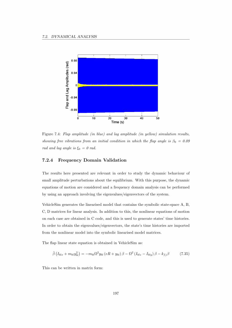
7.2. DYNAMICAL ANALYSIS
Figure 7.4: Flap amplitude (in blue) and lag amplitude (in yellow) simulation results,
showing free vibrations from an initial condition in which the flap angle is β0 = 0.09
rad and lag angle is ξ0 = 0 rad.
7.2.4 Frequency Domain Validation
The results here presented are relevant in order to study the dynamic behaviour of
small amplitude perturbations about the equilibrium. With this purpose, the dynamic
equations of motion are considered and a frequency domain analysis can be performed
by using an approach involving the eigenvalues/eigenvectors of the system.
VehicleSim generates the linearised model that contains the symbolic state-space A, B,
C, D matrices for linear analysis. In addition to this, the nonlinear equations of motion
on each case are obtained in C code, and this is used to generate states’ time histories.
In order to obtain the eigenvalues/eigenvectors, the state’s time histories are imported
from the nonlinear model into the symbolic linearised model matrices.
The flap linear state equation is obtained in VehicleSim as:
β(Iblx +mbly
2bl
)= −mblΩ
2ybl (eR+ ybl)β − Ω2 (Iblz − Ibly)β − kfjβ (7.35)
This can be written in matrix form:
197

7.2. DYNAMICAL ANALYSIS
Figure 7.5: Uncoupled and coupled flap dynamics (red, linear flap simulation results,
blue, nonlinear flap simulation results).
x1
x2
=
0 1
F 0
x1
x2
where x1 = β, x2 = β and F is equal to:
[−kfj −mbly
2blΩ
2 − Ω2eRmblybl + Ω2 (Ibly − Iblz)]/(Iblx +mbly
2bl
)(7.36)
By feeding the matrix with the corresponding physical parameters, the eigenvalues are:
λ1,2 = 0±48.8564i where the complex part of λ1,2 is the flap natural frequency, 48.8564
rad/s slightly above the main rotor’s angular speed as this simulation corresponds to
the case where there is a flap spring kfj , and offset eR 6= 0.
In similar manner, the linear lag equation of motion yields can be written as a first
order system: y1
y2
=
0 1
H G
y1
y2
where y1 = ξ, y2 = ξ and:
H = −(kfj + eRmblΩ
2ybl)/(Iblz +mbly
2bl
)(7.37)
198
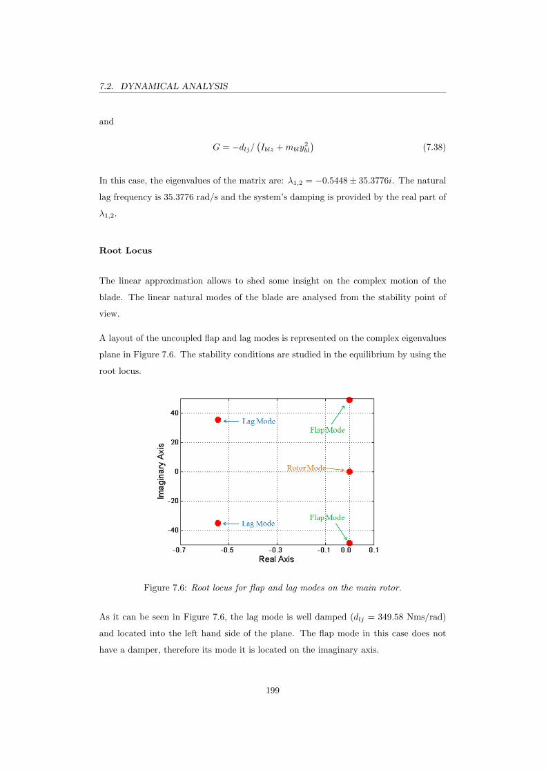
7.2. DYNAMICAL ANALYSIS
and
G = −dlj/(Iblz +mbly
2bl
)(7.38)
In this case, the eigenvalues of the matrix are: λ1,2 = −0.5448± 35.3776i. The natural
lag frequency is 35.3776 rad/s and the system’s damping is provided by the real part of
λ1,2.
Root Locus
The linear approximation allows to shed some insight on the complex motion of the
blade. The linear natural modes of the blade are analysed from the stability point of
view.
A layout of the uncoupled flap and lag modes is represented on the complex eigenvalues
plane in Figure 7.6. The stability conditions are studied in the equilibrium by using the
root locus.
Figure 7.6: Root locus for flap and lag modes on the main rotor.
As it can be seen in Figure 7.6, the lag mode is well damped (dlj = 349.58 Nms/rad)
and located into the left hand side of the plane. The flap mode in this case does not
have a damper, therefore its mode it is located on the imaginary axis.
199
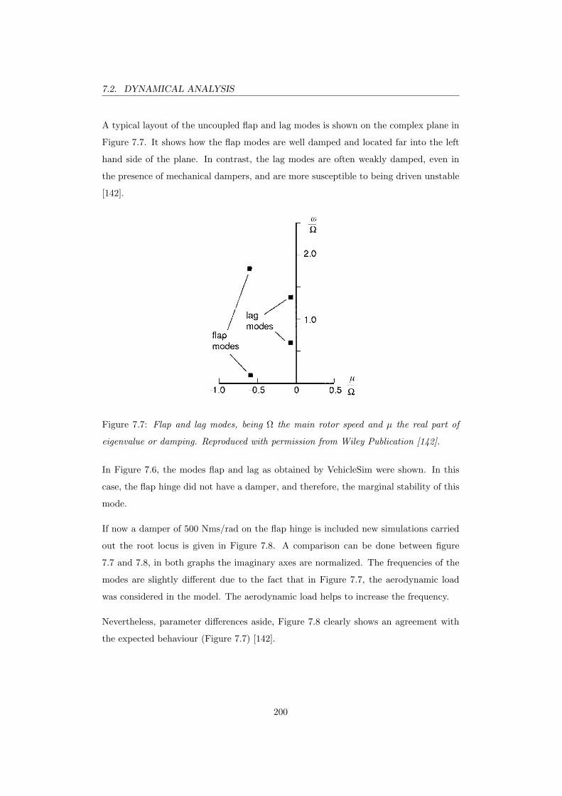
7.2. DYNAMICAL ANALYSIS
A typical layout of the uncoupled flap and lag modes is shown on the complex plane in
Figure 7.7. It shows how the flap modes are well damped and located far into the left
hand side of the plane. In contrast, the lag modes are often weakly damped, even in
the presence of mechanical dampers, and are more susceptible to being driven unstable
[142].
Figure 7.7: Flap and lag modes, being Ω the main rotor speed and µ the real part of
eigenvalue or damping. Reproduced with permission from Wiley Publication [142].
In Figure 7.6, the modes flap and lag as obtained by VehicleSim were shown. In this
case, the flap hinge did not have a damper, and therefore, the marginal stability of this
mode.
If now a damper of 500 Nms/rad on the flap hinge is included new simulations carried
out the root locus is given in Figure 7.8. A comparison can be done between figure
7.7 and 7.8, in both graphs the imaginary axes are normalized. The frequencies of the
modes are slightly different due to the fact that in Figure 7.7, the aerodynamic load
was considered in the model. The aerodynamic load helps to increase the frequency.
Nevertheless, parameter differences aside, Figure 7.8 clearly shows an agreement with
the expected behaviour (Figure 7.7) [142].
200
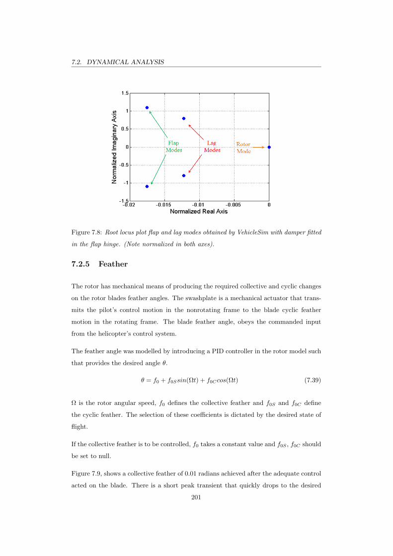
7.2. DYNAMICAL ANALYSIS
Figure 7.8: Root locus plot flap and lag modes obtained by VehicleSim with damper fitted
in the flap hinge. (Note normalized in both axes).
7.2.5 Feather
The rotor has mechanical means of producing the required collective and cyclic changes
on the rotor blades feather angles. The swashplate is a mechanical actuator that trans-
mits the pilot’s control motion in the nonrotating frame to the blade cyclic feather
motion in the rotating frame. The blade feather angle, obeys the commanded input
from the helicopter’s control system.
The feather angle was modelled by introducing a PID controller in the rotor model such
that provides the desired angle θ.
θ = f0 + f0Ssin(Ωt) + f0Ccos(Ωt) (7.39)
Ω is the rotor angular speed, f0 defines the collective feather and f0S and f0C define
the cyclic feather. The selection of these coefficients is dictated by the desired state of
flight.
If the collective feather is to be controlled, f0 takes a constant value and f0S , f0C should
be set to null.
Figure 7.9, shows a collective feather of 0.01 radians achieved after the adequate control
acted on the blade. There is a short peak transient that quickly drops to the desired
201
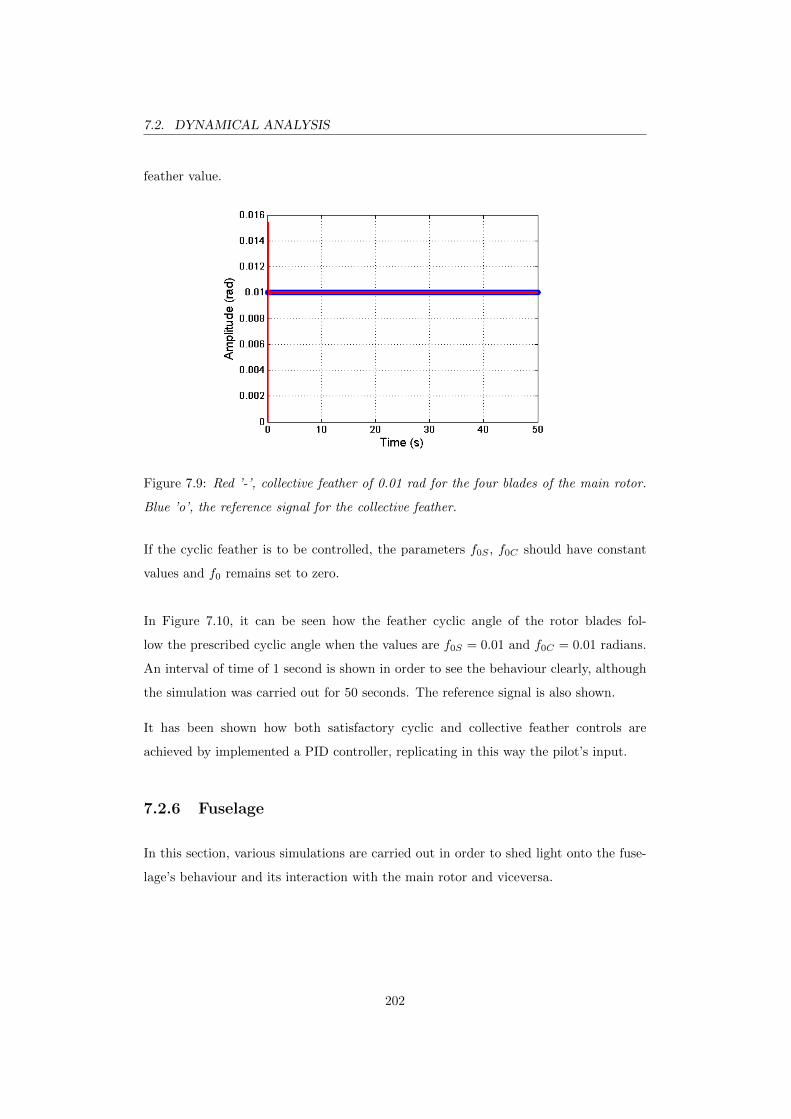
7.2. DYNAMICAL ANALYSIS
feather value.
Figure 7.9: Red ’-’, collective feather of 0.01 rad for the four blades of the main rotor.
Blue ’o’, the reference signal for the collective feather.
If the cyclic feather is to be controlled, the parameters f0S , f0C should have constant
values and f0 remains set to zero.
In Figure 7.10, it can be seen how the feather cyclic angle of the rotor blades fol-
low the prescribed cyclic angle when the values are f0S = 0.01 and f0C = 0.01 radians.
An interval of time of 1 second is shown in order to see the behaviour clearly, although
the simulation was carried out for 50 seconds. The reference signal is also shown.
It has been shown how both satisfactory cyclic and collective feather controls are
achieved by implemented a PID controller, replicating in this way the pilot’s input.
7.2.6 Fuselage
In this section, various simulations are carried out in order to shed light onto the fuse-
lage’s behaviour and its interaction with the main rotor and viceversa.
202
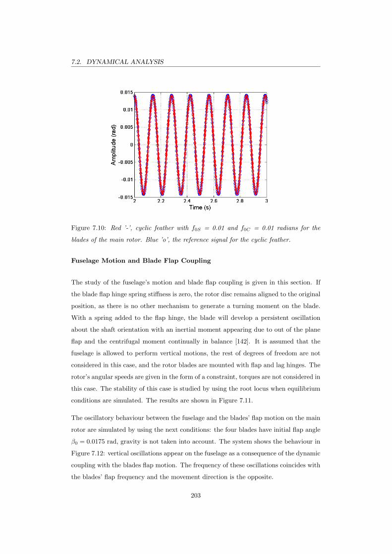
7.2. DYNAMICAL ANALYSIS
Figure 7.10: Red ’-’, cyclic feather with f0S = 0.01 and f0C = 0.01 radians for the
blades of the main rotor. Blue ’o’, the reference signal for the cyclic feather.
Fuselage Motion and Blade Flap Coupling
The study of the fuselage’s motion and blade flap coupling is given in this section. If
the blade flap hinge spring stiffness is zero, the rotor disc remains aligned to the original
position, as there is no other mechanism to generate a turning moment on the blade.
With a spring added to the flap hinge, the blade will develop a persistent oscillation
about the shaft orientation with an inertial moment appearing due to out of the plane
flap and the centrifugal moment continually in balance [142]. It is assumed that the
fuselage is allowed to perform vertical motions, the rest of degrees of freedom are not
considered in this case, and the rotor blades are mounted with flap and lag hinges. The
rotor’s angular speeds are given in the form of a constraint, torques are not considered in
this case. The stability of this case is studied by using the root locus when equilibrium
conditions are simulated. The results are shown in Figure 7.11.
The oscillatory behaviour between the fuselage and the blades’ flap motion on the main
rotor are simulated by using the next conditions: the four blades have initial flap angle
β0 = 0.0175 rad, gravity is not taken into account. The system shows the behaviour in
Figure 7.12: vertical oscillations appear on the fuselage as a consequence of the dynamic
coupling with the blades flap motion. The frequency of these oscillations coincides with
the blades’ flap frequency and the movement direction is the opposite.
203
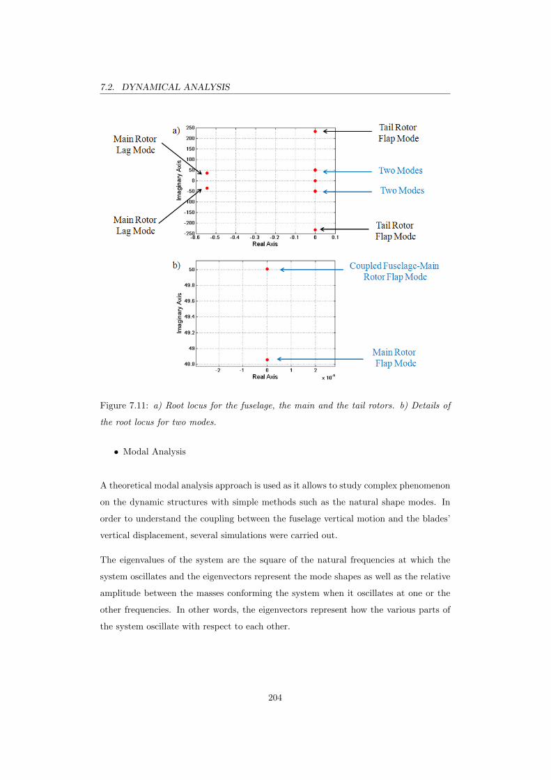
7.2. DYNAMICAL ANALYSIS
Figure 7.11: a) Root locus for the fuselage, the main and the tail rotors. b) Details of
the root locus for two modes.
• Modal Analysis
A theoretical modal analysis approach is used as it allows to study complex phenomenon
on the dynamic structures with simple methods such as the natural shape modes. In
order to understand the coupling between the fuselage vertical motion and the blades’
vertical displacement, several simulations were carried out.
The eigenvalues of the system are the square of the natural frequencies at which the
system oscillates and the eigenvectors represent the mode shapes as well as the relative
amplitude between the masses conforming the system when it oscillates at one or the
other frequencies. In other words, the eigenvectors represent how the various parts of
the system oscillate with respect to each other.
204

7.2. DYNAMICAL ANALYSIS
Figure 7.12: Coupled movement for the fuselage and the main rotor along the vertical
axis. Solid red line, fuselage. Dotted blue line, flap.
This section is based on the mathematical analysis of the linearised model. In general,
it is well known that the eigenvalues, λ, of a matrix A satisfy the equation:
(A− λI)φ = 0 (7.40)
being φ an eigenvector.
The solution of the algebraic equation (7.40) is:
det (A− λI) = 0 (7.41)
The corresponding eigenvectors, are obtained for any eigenvalue λi by:
Aφi = λiφi (7.42)
The elements of the eigenvectors give a measure of the relative activity of the state
variables when a particular mode is excited. In other words, the i-th element of the
eigenvector φi measures the activity of the state variable xi in the i-th eigenvalue [142],
[149].
The mathematical model of the system under study has twenty four state variables,
q(t) = x1, x2, x3, ..., x24T where the first variable x1 describes the fuselage’s vertical
translation, x2 describes the main rotor rotation, x3, x5, x7 and x9 describe the flap
angle for the first, second, third and fourth blades on the main rotor, respectively. x4,
x6, x8 and x10 describe the lag angle for the first second, third and fourth blade on the
main rotor, respectively. x11 describes the angular displacement of the tail rotor, x12
205
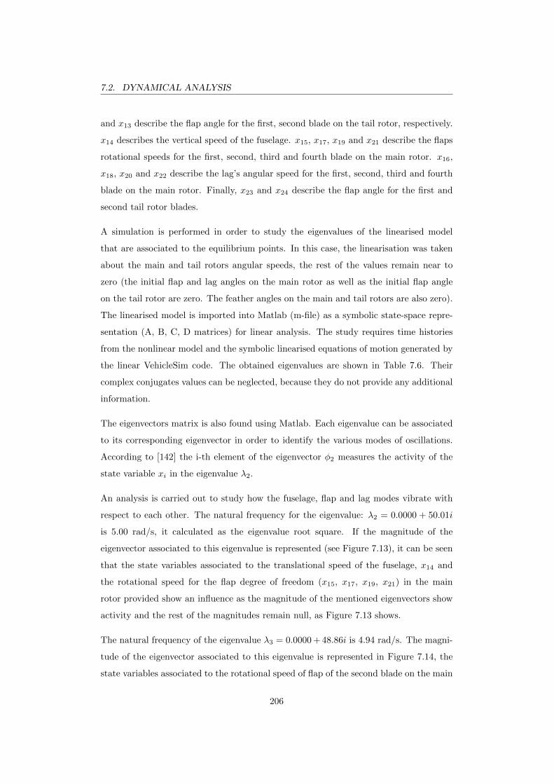
7.2. DYNAMICAL ANALYSIS
and x13 describe the flap angle for the first, second blade on the tail rotor, respectively.
x14 describes the vertical speed of the fuselage. x15, x17, x19 and x21 describe the flaps
rotational speeds for the first, second, third and fourth blade on the main rotor. x16,
x18, x20 and x22 describe the lag’s angular speed for the first, second, third and fourth
blade on the main rotor. Finally, x23 and x24 describe the flap angle for the first and
second tail rotor blades.
A simulation is performed in order to study the eigenvalues of the linearised model
that are associated to the equilibrium points. In this case, the linearisation was taken
about the main and tail rotors angular speeds, the rest of the values remain near to
zero (the initial flap and lag angles on the main rotor as well as the initial flap angle
on the tail rotor are zero. The feather angles on the main and tail rotors are also zero).
The linearised model is imported into Matlab (m-file) as a symbolic state-space repre-
sentation (A, B, C, D matrices) for linear analysis. The study requires time histories
from the nonlinear model and the symbolic linearised equations of motion generated by
the linear VehicleSim code. The obtained eigenvalues are shown in Table 7.6. Their
complex conjugates values can be neglected, because they do not provide any additional
information.
The eigenvectors matrix is also found using Matlab. Each eigenvalue can be associated
to its corresponding eigenvector in order to identify the various modes of oscillations.
According to [142] the i-th element of the eigenvector φ2 measures the activity of the
state variable xi in the eigenvalue λ2.
An analysis is carried out to study how the fuselage, flap and lag modes vibrate with
respect to each other. The natural frequency for the eigenvalue: λ2 = 0.0000 + 50.01i
is 5.00 rad/s, it calculated as the eigenvalue root square. If the magnitude of the
eigenvector associated to this eigenvalue is represented (see Figure 7.13), it can be seen
that the state variables associated to the translational speed of the fuselage, x14 and
the rotational speed for the flap degree of freedom (x15, x17, x19, x21) in the main
rotor provided show an influence as the magnitude of the mentioned eigenvectors show
activity and the rest of the magnitudes remain null, as Figure 7.13 shows.
The natural frequency of the eigenvalue λ3 = 0.0000 + 48.86i is 4.94 rad/s. The magni-
tude of the eigenvector associated to this eigenvalue is represented in Figure 7.14, the
state variables associated to the rotational speed of flap of the second blade on the main
206
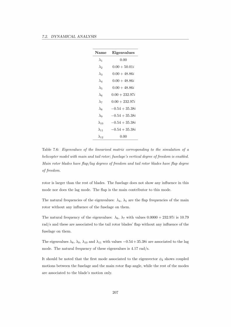
7.2. DYNAMICAL ANALYSIS
Name Eigenvalues
λ1 0.00
λ2 0.00 + 50.01i
λ3 0.00 + 48.86i
λ4 0.00 + 48.86i
λ5 0.00 + 48.86i
λ6 0.00 + 232.97i
λ7 0.00 + 232.97i
λ8 −0.54 + 35.38i
λ9 −0.54 + 35.38i
λ10 −0.54 + 35.38i
λ11 −0.54 + 35.38i
λ12 0.00
Table 7.6: Eigenvalues of the linearised matrix corresponding to the simulation of a
helicopter model with main and tail rotor; fuselage’s vertical degree of freedom is enabled.
Main rotor blades have flap/lag degrees of freedom and tail rotor blades have flap degree
of freedom.
rotor is larger than the rest of blades. The fuselage does not show any influence in this
mode nor does the lag mode. The flap is the main contributor to this mode.
The natural frequencies of the eigenvalues: λ4, λ5 are the flap frequencies of the main
rotor without any influence of the fuselage on them.
The natural frequency of the eigenvalues: λ6, λ7 with values 0.0000 + 232.97i is 10.79
rad/s and these are associated to the tail rotor blades’ flap without any influence of the
fuselage on them.
The eigenvalues λ8, λ9, λ10 and λ11 with values −0.54 + 35.38i are associated to the lag
mode. The natural frequency of these eigenvalues is 4.17 rad/s.
It should be noted that the first mode associated to the eigenvector φ2 shows coupled
motions between the fuselage and the main rotor flap angle, while the rest of the modes
are associated to the blade’s motion only.
207

7.2. DYNAMICAL ANALYSIS
Figure 7.13: Magnitude of the eigenvector associated to the eigenvalue λ2 = 0.0 + 50.01i
and its influence on the state variables.
If a comparison between the natural frequencies related to mode 1 (coupled fuselage-flap
φ2) and mode 2 associated to eigenvector φ3 is done, it is found that their values are
similar. As a consequence of this, a coupling between these two modes when the natural
frequencies change as a function of the mass ratio is expected. The next part in this
section will focus on validating this expectation.
The influence of the mass ratio on the coupled modes is given as massblade/massfuselage.
If the blade’s mass is 31.06 kg and the fuselage’s mass is 2063.336 kg, the mass ratio is
0.015. As it can be seen in Figure 7.15, the difference between the frequencies associated
to mode 1 and mode 2 is small in this case. However, the mass ratio increases the
difference between the natural frequencies associated to mode 1 and mode 2. The
fuselage’s mass decreases from 2063.336 kg to 863.336 kg and the blades’ masses increase
from 31.06 kg to 34.06 kg, respectively. In Figure 7.15, the behaviour shows the influence
of mass ratio on these coupled modes through the change of natural frequencies as a
function of the mass ratio.
As the mass ratio is increased, the coupling between the fuselage and flap becomes
larger. Conversely, if the mass ratio decreases, the coupling is reduced.
208
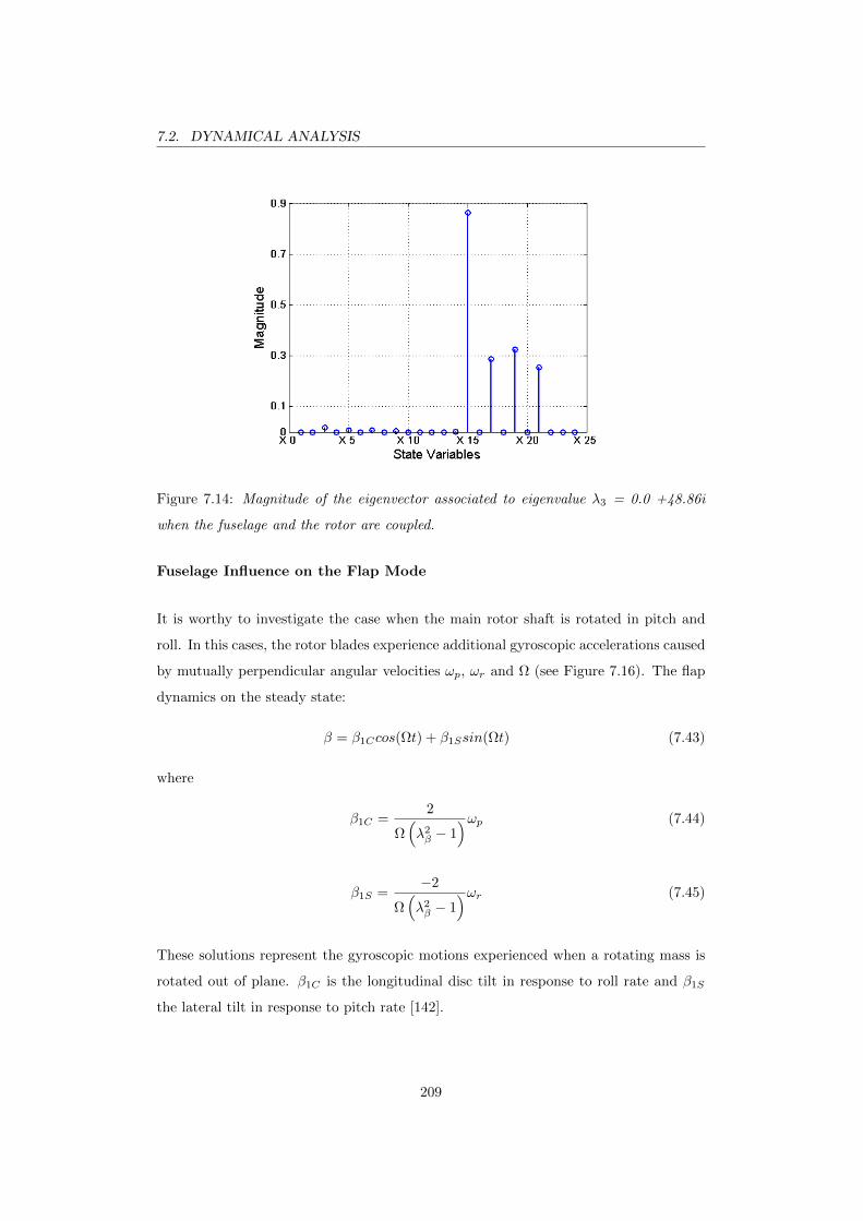
7.2. DYNAMICAL ANALYSIS
Figure 7.14: Magnitude of the eigenvector associated to eigenvalue λ3 = 0.0 +48.86i
when the fuselage and the rotor are coupled.
Fuselage Influence on the Flap Mode
It is worthy to investigate the case when the main rotor shaft is rotated in pitch and
roll. In this cases, the rotor blades experience additional gyroscopic accelerations caused
by mutually perpendicular angular velocities ωp, ωr and Ω (see Figure 7.16). The flap
dynamics on the steady state:
β = β1Ccos(Ωt) + β1Ssin(Ωt) (7.43)
where
β1C =2
Ω(λ2β − 1
)ωp (7.44)
β1S =−2
Ω(λ2β − 1
)ωr (7.45)
These solutions represent the gyroscopic motions experienced when a rotating mass is
rotated out of plane. β1C is the longitudinal disc tilt in response to roll rate and β1S
the lateral tilt in response to pitch rate [142].
209

7.2. DYNAMICAL ANALYSIS
Figure 7.15: Mode 1, blue ’+’, mode 2, red ’•’. Influence of mass ratio on these
coupled modes. Change of natural frequencies as a function of the mass ratio
massblade/massfuselage.
Based on the previous considerations, if now a torque is introduced around the Y axis
on the fuselage producing a pitch rotation and the initial flap angles on the blades are
zero, this will be transmitted through the shaft to the flap hinges on each blade. The
torque is included in the VehicleSim model as a step function, its magnitude being 1750
N·m. In here, flap hinges are included in the model to allow for the flap degree of
freedom, but neither lag hinges nor tail rotor have been included in the model because
this section is focused in the analysis of the interaction between the fuselage and the
flap only. The main rotor rotational speed is described in VehicleSim as a constraint.
The impact of the fuselage’s pitch and roll on the flap dynamics are calculated by using
the expression (7.43) where λ2β = 1.2 is a standard value applicable to this model [142].
It is expected that the flap on the four blades behaves accordingly to the fuselage’s
displacement. Figure 7.17 shows the blade flap angle, in blue. In red, the expected flap
angle is shown.
It has been shown how an induced flap motion can be introduced by the fuselage’s
roll/pitch rate, as it was expected from the theory.
210

7.2. DYNAMICAL ANALYSIS
Figure 7.16: Sketch of main rotor and gyroscopic moments in vacuum. This figure is
plotted by the author and based on [142].
Lag Mode Influence on the Fuselage
In order to establish new a test for model’s validation purposes, the interaction between
the flap and fuselage motion and the lag is studied. Due to the roll and pitch of the
fuselage, the associated acceleration of the hub contributes with inertial terms to the lag
equations. However, blade flap takes place in this case, and the corresponding Coriolis
inertia terms must be also included. The inertia of the blades’ lag causes further pitching
and rolling moments on the helicopter [141].
The previous assumptions suggest the following validation test: if two torques around
the fuselage’s X and Y axes are considered, the fuselage will experience roll and pitch
motions. The effects of these will be transmitted through the rotor shaft onto the blades.
In order to test this behaviour in the VehicleSim model, the corresponding torques are
included as pulse functions, their magnitudes are 500 N·m from t = 0 to t = 1 s. The
main rotor rotational speed is given in the form of a constraint. In Figure 7.18, the
spectrums for the roll and pitch motions appearing in the fuselage as a consequence
of the impulses are shown. In blue, both cases are shown when the lag motion is not
considered. In red, the pitch and the roll of the fuselage when the lag is taken into
account in the model.
211
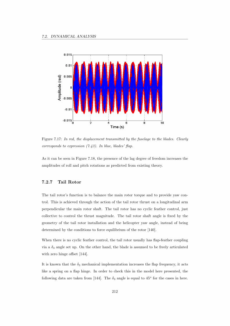
7.2. DYNAMICAL ANALYSIS
Figure 7.17: In red, the displacement transmitted by the fuselage to the blades. Clearly
corresponds to expression (7.43). In blue, blades’ flap.
As it can be seen in Figure 7.18, the presence of the lag degree of freedom increases the
amplitudes of roll and pitch rotations as predicted from existing theory.
7.2.7 Tail Rotor
The tail rotor’s function is to balance the main rotor torque and to provide yaw con-
trol. This is achieved through the action of the tail rotor thrust on a longitudinal arm
perpendicular the main rotor shaft. The tail rotor has no cyclic feather control, just
collective to control the thrust magnitude. The tail rotor shaft angle is fixed by the
geometry of the tail rotor installation and the helicopter yaw angle, instead of being
determined by the conditions to force equilibrium of the rotor [140].
When there is no cyclic feather control, the tail rotor usually has flap-feather coupling
via a δ3 angle set up. On the other hand, the blade is assumed to be freely articulated
with zero hinge offset [144].
It is known that the δ3 mechanical implementation increases the flap frequency, it acts
like a spring on a flap hinge. In order to check this in the model here presented, the
following data are taken from [144]. The δ3 angle is equal to 45o for the cases in here.
212
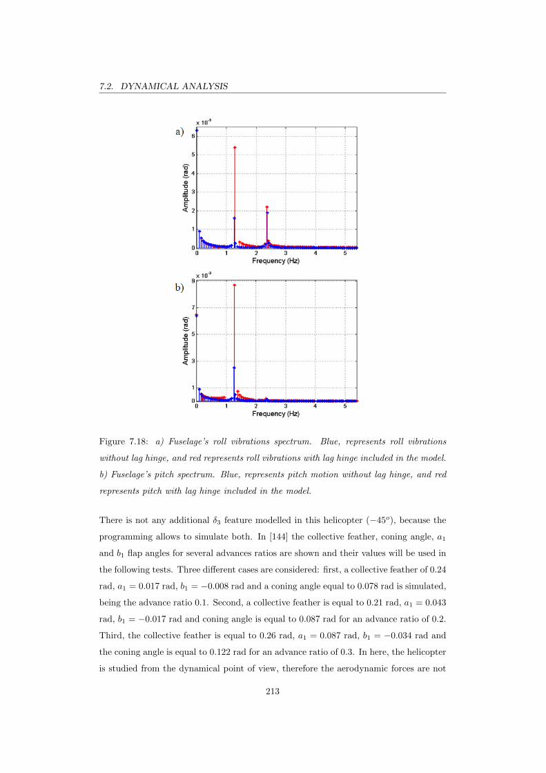
7.2. DYNAMICAL ANALYSIS
Figure 7.18: a) Fuselage’s roll vibrations spectrum. Blue, represents roll vibrations
without lag hinge, and red represents roll vibrations with lag hinge included in the model.
b) Fuselage’s pitch spectrum. Blue, represents pitch motion without lag hinge, and red
represents pitch with lag hinge included in the model.
There is not any additional δ3 feature modelled in this helicopter (−45o), because the
programming allows to simulate both. In [144] the collective feather, coning angle, a1
and b1 flap angles for several advances ratios are shown and their values will be used in
the following tests. Three different cases are considered: first, a collective feather of 0.24
rad, a1 = 0.017 rad, b1 = −0.008 rad and a coning angle equal to 0.078 rad is simulated,
being the advance ratio 0.1. Second, a collective feather is equal to 0.21 rad, a1 = 0.043
rad, b1 = −0.017 rad and coning angle is equal to 0.087 rad for an advance ratio of 0.2.
Third, the collective feather is equal to 0.26 rad, a1 = 0.087 rad, b1 = −0.034 rad and
the coning angle is equal to 0.122 rad for an advance ratio of 0.3. In here, the helicopter
is studied from the dynamical point of view, therefore the aerodynamic forces are not
213
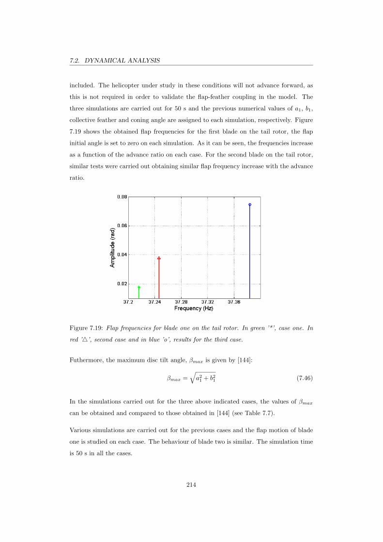
7.2. DYNAMICAL ANALYSIS
included. The helicopter under study in these conditions will not advance forward, as
this is not required in order to validate the flap-feather coupling in the model. The
three simulations are carried out for 50 s and the previous numerical values of a1, b1,
collective feather and coning angle are assigned to each simulation, respectively. Figure
7.19 shows the obtained flap frequencies for the first blade on the tail rotor, the flap
initial angle is set to zero on each simulation. As it can be seen, the frequencies increase
as a function of the advance ratio on each case. For the second blade on the tail rotor,
similar tests were carried out obtaining similar flap frequency increase with the advance
ratio.
Figure 7.19: Flap frequencies for blade one on the tail rotor. In green ’*’, case one. In
red ’4’, second case and in blue ’o’, results for the third case.
Futhermore, the maximum disc tilt angle, βmax is given by [144]:
βmax =√a2
1 + b21 (7.46)
In the simulations carried out for the three above indicated cases, the values of βmax
can be obtained and compared to those obtained in [144] (see Table 7.7).
Various simulations are carried out for the previous cases and the flap motion of blade
one is studied on each case. The behaviour of blade two is similar. The simulation time
is 50 s in all the cases.
214
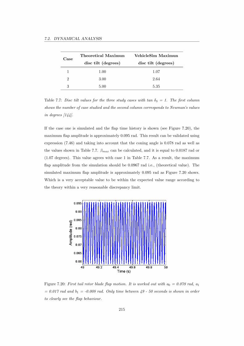
7.2. DYNAMICAL ANALYSIS
CaseTheoretical Maximun
disc tilt (degrees)
VehicleSim Maximun
disc tilt (degrees)
1 1.00 1.07
2 3.00 2.64
3 5.00 5.35
Table 7.7: Disc tilt values for the three study cases with tan δ3 = 1. The first column
shows the number of case studied and the second column corresponds to Newman’s values
in degrees [144].
If the case one is simulated and the flap time history is shown (see Figure 7.20), the
maximum flap amplitude is approximately 0.095 rad. This result can be validated using
expression (7.46) and taking into account that the coning angle is 0.078 rad as well as
the values shown in Table 7.7. βmax can be calculated, and it is equal to 0.0187 rad or
(1.07 degrees). This value agrees with case 1 in Table 7.7. As a result, the maximum
flap amplitude from the simulation should be 0.0967 rad i.e., (theoretical value). The
simulated maximum flap amplitude is approximately 0.095 rad as Figure 7.20 shows.
Which is a very acceptable value to be within the expected value range according to
the theory within a very reasonable discrepancy limit.
Figure 7.20: First tail rotor blade flap motion. It is worked out with a0 = 0.078 rad, a1
= 0.017 rad and b1 = -0.008 rad. Only time between 49 - 50 seconds is shown in order
to clearly see the flap behaviour.
215
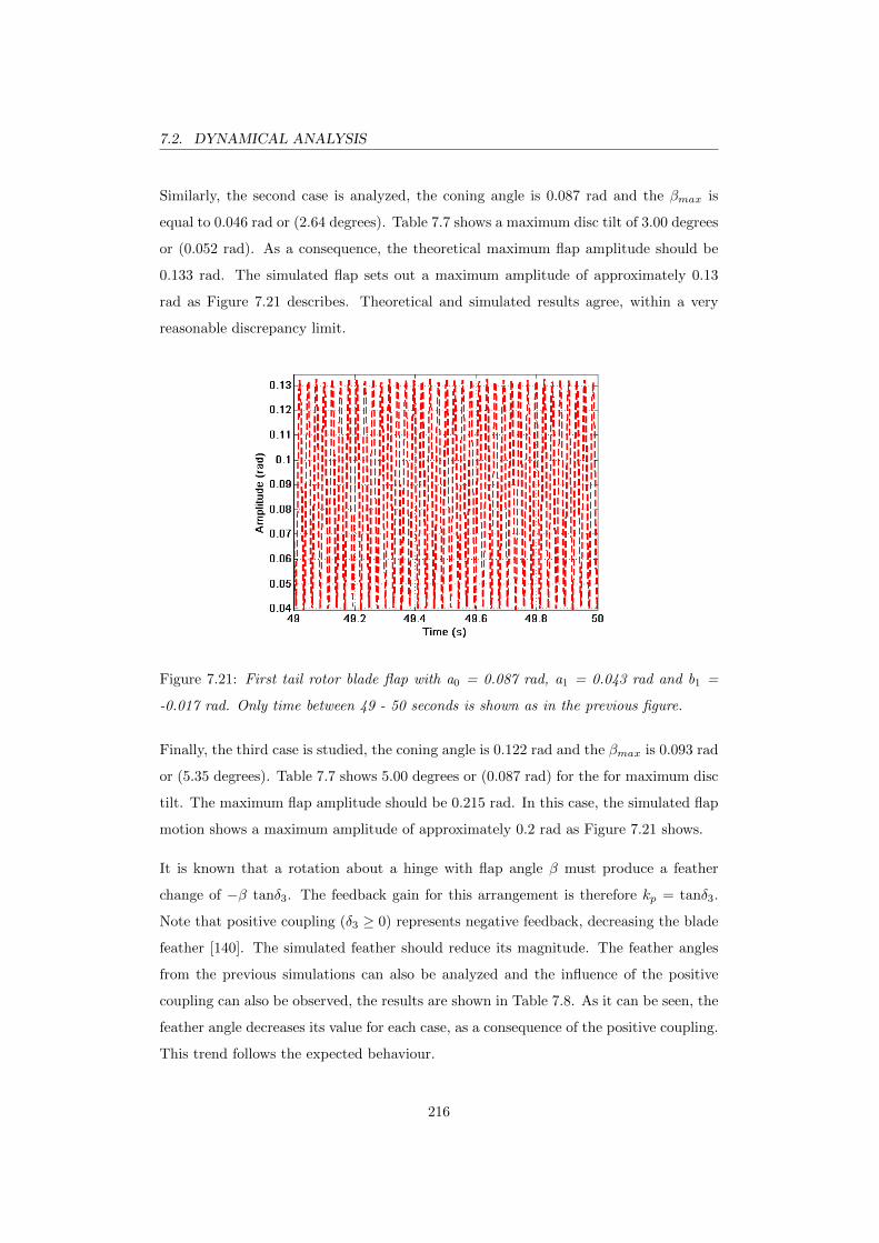
7.2. DYNAMICAL ANALYSIS
Similarly, the second case is analyzed, the coning angle is 0.087 rad and the βmax is
equal to 0.046 rad or (2.64 degrees). Table 7.7 shows a maximum disc tilt of 3.00 degrees
or (0.052 rad). As a consequence, the theoretical maximum flap amplitude should be
0.133 rad. The simulated flap sets out a maximum amplitude of approximately 0.13
rad as Figure 7.21 describes. Theoretical and simulated results agree, within a very
reasonable discrepancy limit.
Figure 7.21: First tail rotor blade flap with a0 = 0.087 rad, a1 = 0.043 rad and b1 =
-0.017 rad. Only time between 49 - 50 seconds is shown as in the previous figure.
Finally, the third case is studied, the coning angle is 0.122 rad and the βmax is 0.093 rad
or (5.35 degrees). Table 7.7 shows 5.00 degrees or (0.087 rad) for the for maximum disc
tilt. The maximum flap amplitude should be 0.215 rad. In this case, the simulated flap
motion shows a maximum amplitude of approximately 0.2 rad as Figure 7.21 shows.
It is known that a rotation about a hinge with flap angle β must produce a feather
change of −β tanδ3. The feedback gain for this arrangement is therefore kp = tanδ3.
Note that positive coupling (δ3 ≥ 0) represents negative feedback, decreasing the blade
feather [140]. The simulated feather should reduce its magnitude. The feather angles
from the previous simulations can also be analyzed and the influence of the positive
coupling can also be observed, the results are shown in Table 7.8. As it can be seen, the
feather angle decreases its value for each case, as a consequence of the positive coupling.
This trend follows the expected behaviour.
216
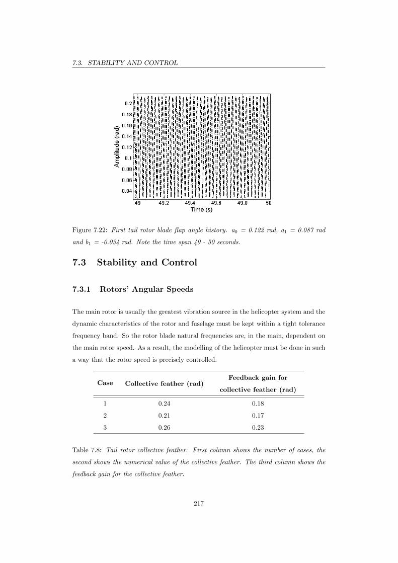
7.3. STABILITY AND CONTROL
Figure 7.22: First tail rotor blade flap angle history. a0 = 0.122 rad, a1 = 0.087 rad
and b1 = -0.034 rad. Note the time span 49 - 50 seconds.
7.3 Stability and Control
7.3.1 Rotors’ Angular Speeds
The main rotor is usually the greatest vibration source in the helicopter system and the
dynamic characteristics of the rotor and fuselage must be kept within a tight tolerance
frequency band. So the rotor blade natural frequencies are, in the main, dependent on
the main rotor speed. As a result, the modelling of the helicopter must be done in such
a way that the rotor speed is precisely controlled.
Case Collective feather (rad)Feedback gain for
collective feather (rad)
1 0.24 0.18
2 0.21 0.17
3 0.26 0.23
Table 7.8: Tail rotor collective feather. First column shows the number of cases, the
second shows the numerical value of the collective feather. The third column shows the
feedback gain for the collective feather.
217

7.3. STABILITY AND CONTROL
The control moments must be developed by the rotors and they depend of the equilib-
rium conditions on the helicopter. The balance of forces and moments determine the
action of the rotor with respect to the fuselage [144]. The tail rotor propulsive force is
included in the overall airframe drag and is balanced by the main rotor [140].
The control of the engine is normally performed by means of a fuel valve, therefore the
governor must sense a change in the rotor speed brought about by a change in torque
demand and adjust the fuel valve accordingly. This behaviour continues until engine
torque and rotor torque demands are balanced [144].
The tail rotor gearing is chosen to be 5.25 according to [142]. In this model, this is
implemented by two PID controllers; (as described in Chapter 5). The PID controller
input, the reference value for the main rotor angular speed, is 44.4 rad/s and in the case
of the tail rotor is 5.25·44.4 rad/s. The PID outputs are the rotational speeds of the main
and tail rotors respectively. A simulation is carried out under the following conditions,
the feather angles (cyclic and collective) are zero as well as the collective feather angle
on the tail rotor. The flap and lag degrees of freedom do not have initial condition i.e.,
β0 = 0 rad and ξ0 = 0 rad. The tail rotor initial flap angle is also zero. Figure 7.23
shows the obtained angular speeds for both rotors as well as the corresponding control
signal.
Figure 7.23: Angular speeds on both rotors. In blue, main rotor speed. In red, tail rotor
speed. The control signals are shown on both cases, and clearly the speeds successfully
follow the respective reference speeds.
218
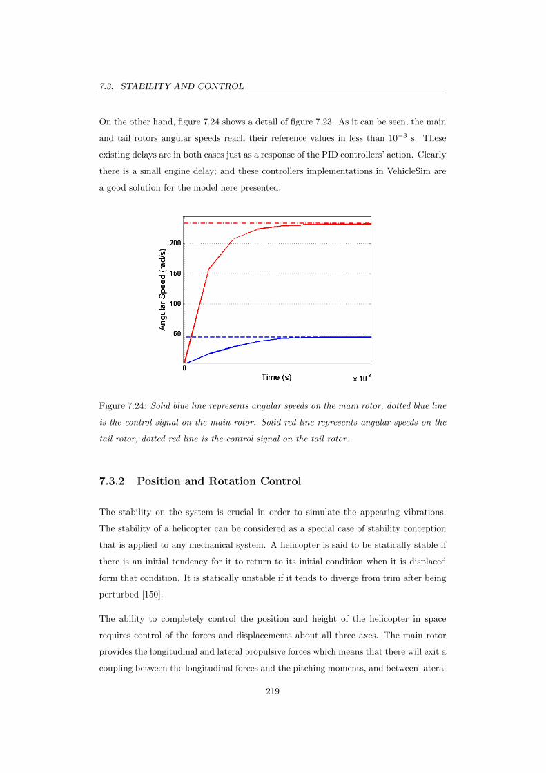
7.3. STABILITY AND CONTROL
On the other hand, figure 7.24 shows a detail of figure 7.23. As it can be seen, the main
and tail rotors angular speeds reach their reference values in less than 10−3 s. These
existing delays are in both cases just as a response of the PID controllers’ action. Clearly
there is a small engine delay; and these controllers implementations in VehicleSim are
a good solution for the model here presented.
Figure 7.24: Solid blue line represents angular speeds on the main rotor, dotted blue line
is the control signal on the main rotor. Solid red line represents angular speeds on the
tail rotor, dotted red line is the control signal on the tail rotor.
7.3.2 Position and Rotation Control
The stability on the system is crucial in order to simulate the appearing vibrations.
The stability of a helicopter can be considered as a special case of stability conception
that is applied to any mechanical system. A helicopter is said to be statically stable if
there is an initial tendency for it to return to its initial condition when it is displaced
form that condition. It is statically unstable if it tends to diverge from trim after being
perturbed [150].
The ability to completely control the position and height of the helicopter in space
requires control of the forces and displacements about all three axes. The main rotor
provides the longitudinal and lateral propulsive forces which means that there will exit a
coupling between the longitudinal forces and the pitching moments, and between lateral
219
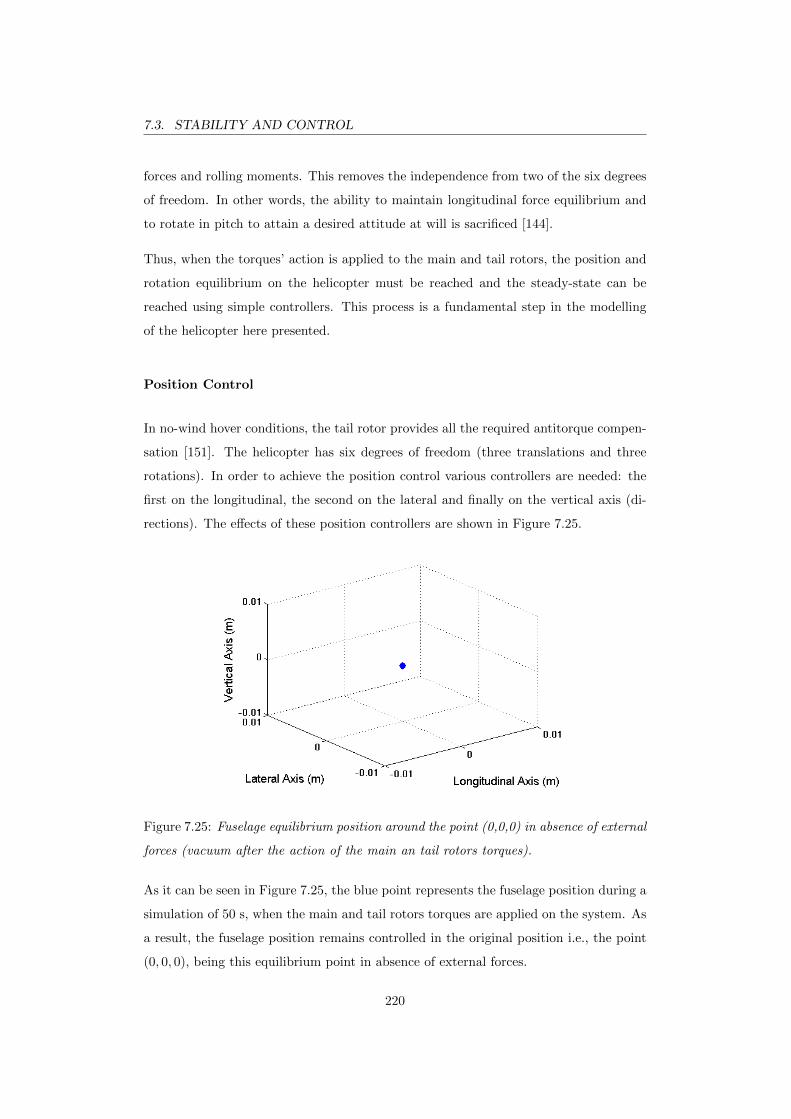
7.3. STABILITY AND CONTROL
forces and rolling moments. This removes the independence from two of the six degrees
of freedom. In other words, the ability to maintain longitudinal force equilibrium and
to rotate in pitch to attain a desired attitude at will is sacrificed [144].
Thus, when the torques’ action is applied to the main and tail rotors, the position and
rotation equilibrium on the helicopter must be reached and the steady-state can be
reached using simple controllers. This process is a fundamental step in the modelling
of the helicopter here presented.
Position Control
In no-wind hover conditions, the tail rotor provides all the required antitorque compen-
sation [151]. The helicopter has six degrees of freedom (three translations and three
rotations). In order to achieve the position control various controllers are needed: the
first on the longitudinal, the second on the lateral and finally on the vertical axis (di-
rections). The effects of these position controllers are shown in Figure 7.25.
Figure 7.25: Fuselage equilibrium position around the point (0,0,0) in absence of external
forces (vacuum after the action of the main an tail rotors torques).
As it can be seen in Figure 7.25, the blue point represents the fuselage position during a
simulation of 50 s, when the main and tail rotors torques are applied on the system. As
a result, the fuselage position remains controlled in the original position i.e., the point
(0, 0, 0), being this equilibrium point in absence of external forces.
220
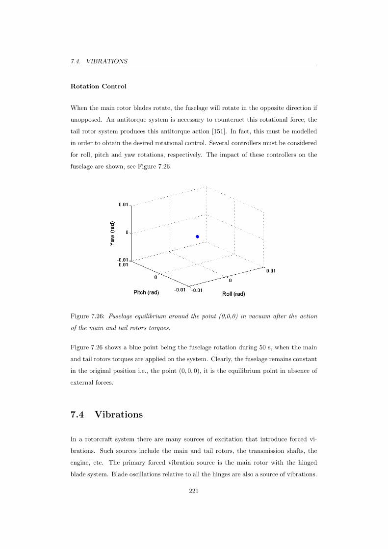
7.4. VIBRATIONS
Rotation Control
When the main rotor blades rotate, the fuselage will rotate in the opposite direction if
unopposed. An antitorque system is necessary to counteract this rotational force, the
tail rotor system produces this antitorque action [151]. In fact, this must be modelled
in order to obtain the desired rotational control. Several controllers must be considered
for roll, pitch and yaw rotations, respectively. The impact of these controllers on the
fuselage are shown, see Figure 7.26.
Figure 7.26: Fuselage equilibrium around the point (0,0,0) in vacuum after the action
of the main and tail rotors torques.
Figure 7.26 shows a blue point being the fuselage rotation during 50 s, when the main
and tail rotors torques are applied on the system. Clearly, the fuselage remains constant
in the original position i.e., the point (0, 0, 0), it is the equilibrium point in absence of
external forces.
7.4 Vibrations
In a rotorcraft system there are many sources of excitation that introduce forced vi-
brations. Such sources include the main and tail rotors, the transmission shafts, the
engine, etc. The primary forced vibration source is the main rotor with the hinged
blade system. Blade oscillations relative to all the hinges are also a source of vibrations.
221
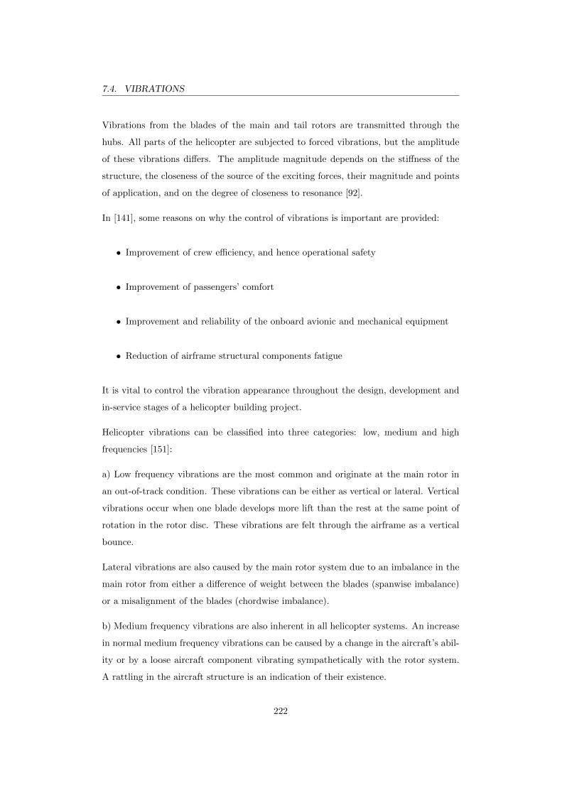
7.4. VIBRATIONS
Vibrations from the blades of the main and tail rotors are transmitted through the
hubs. All parts of the helicopter are subjected to forced vibrations, but the amplitude
of these vibrations differs. The amplitude magnitude depends on the stiffness of the
structure, the closeness of the source of the exciting forces, their magnitude and points
of application, and on the degree of closeness to resonance [92].
In [141], some reasons on why the control of vibrations is important are provided:
• Improvement of crew efficiency, and hence operational safety
• Improvement of passengers’ comfort
• Improvement and reliability of the onboard avionic and mechanical equipment
• Reduction of airframe structural components fatigue
It is vital to control the vibration appearance throughout the design, development and
in-service stages of a helicopter building project.
Helicopter vibrations can be classified into three categories: low, medium and high
frequencies [151]:
a) Low frequency vibrations are the most common and originate at the main rotor in
an out-of-track condition. These vibrations can be either as vertical or lateral. Vertical
vibrations occur when one blade develops more lift than the rest at the same point of
rotation in the rotor disc. These vibrations are felt through the airframe as a vertical
bounce.
Lateral vibrations are also caused by the main rotor system due to an imbalance in the
main rotor from either a difference of weight between the blades (spanwise imbalance)
or a misalignment of the blades (chordwise imbalance).
b) Medium frequency vibrations are also inherent in all helicopter systems. An increase
in normal medium frequency vibrations can be caused by a change in the aircraft’s abil-
ity or by a loose aircraft component vibrating sympathetically with the rotor system.
A rattling in the aircraft structure is an indication of their existence.
222
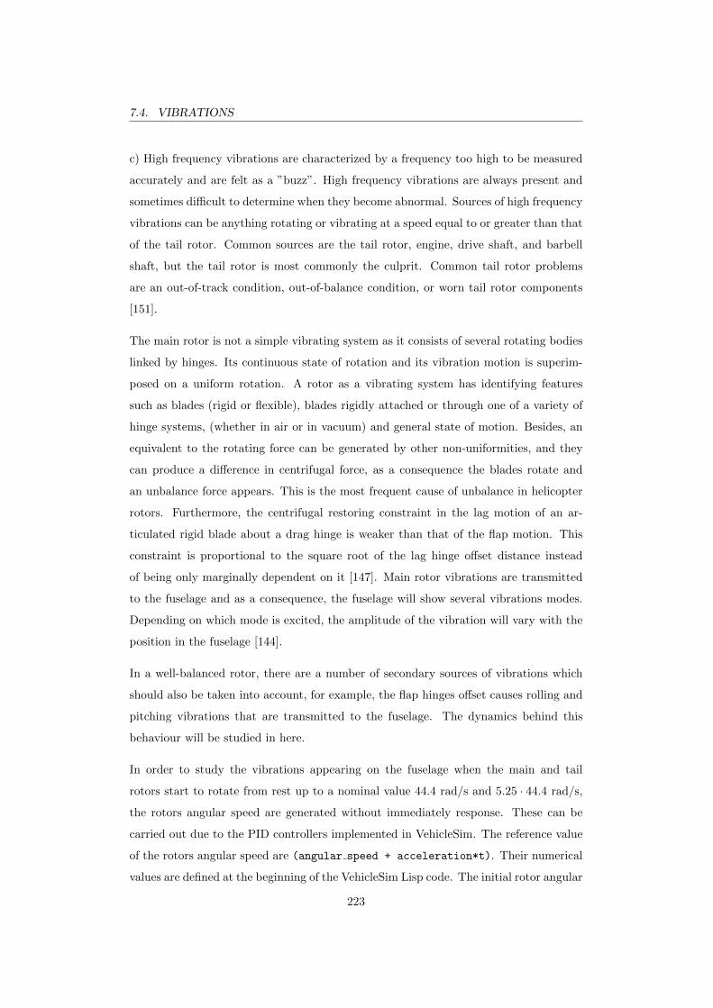
7.4. VIBRATIONS
c) High frequency vibrations are characterized by a frequency too high to be measured
accurately and are felt as a ”buzz”. High frequency vibrations are always present and
sometimes difficult to determine when they become abnormal. Sources of high frequency
vibrations can be anything rotating or vibrating at a speed equal to or greater than that
of the tail rotor. Common sources are the tail rotor, engine, drive shaft, and barbell
shaft, but the tail rotor is most commonly the culprit. Common tail rotor problems
are an out-of-track condition, out-of-balance condition, or worn tail rotor components
[151].
The main rotor is not a simple vibrating system as it consists of several rotating bodies
linked by hinges. Its continuous state of rotation and its vibration motion is superim-
posed on a uniform rotation. A rotor as a vibrating system has identifying features
such as blades (rigid or flexible), blades rigidly attached or through one of a variety of
hinge systems, (whether in air or in vacuum) and general state of motion. Besides, an
equivalent to the rotating force can be generated by other non-uniformities, and they
can produce a difference in centrifugal force, as a consequence the blades rotate and
an unbalance force appears. This is the most frequent cause of unbalance in helicopter
rotors. Furthermore, the centrifugal restoring constraint in the lag motion of an ar-
ticulated rigid blade about a drag hinge is weaker than that of the flap motion. This
constraint is proportional to the square root of the lag hinge offset distance instead
of being only marginally dependent on it [147]. Main rotor vibrations are transmitted
to the fuselage and as a consequence, the fuselage will show several vibrations modes.
Depending on which mode is excited, the amplitude of the vibration will vary with the
position in the fuselage [144].
In a well-balanced rotor, there are a number of secondary sources of vibrations which
should also be taken into account, for example, the flap hinges offset causes rolling and
pitching vibrations that are transmitted to the fuselage. The dynamics behind this
behaviour will be studied in here.
In order to study the vibrations appearing on the fuselage when the main and tail
rotors start to rotate from rest up to a nominal value 44.4 rad/s and 5.25 · 44.4 rad/s,
the rotors angular speed are generated without immediately response. These can be
carried out due to the PID controllers implemented in VehicleSim. The reference value
of the rotors angular speed are (angular speed + acceleration*t). Their numerical
values are defined at the beginning of the VehicleSim Lisp code. The initial rotor angular
223
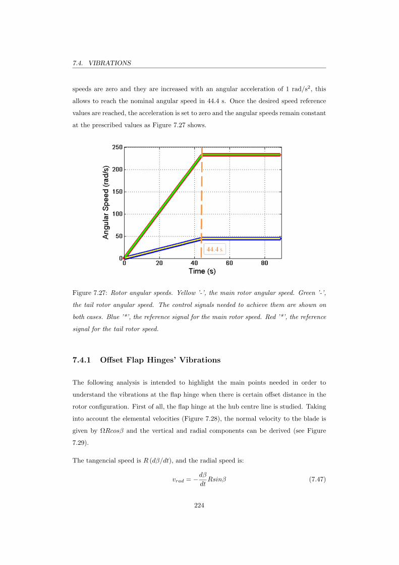
7.4. VIBRATIONS
speeds are zero and they are increased with an angular acceleration of 1 rad/s2, this
allows to reach the nominal angular speed in 44.4 s. Once the desired speed reference
values are reached, the acceleration is set to zero and the angular speeds remain constant
at the prescribed values as Figure 7.27 shows.
Figure 7.27: Rotor angular speeds. Yellow ’-’, the main rotor angular speed. Green ’-’,
the tail rotor angular speed. The control signals needed to achieve them are shown on
both cases. Blue ’*’, the reference signal for the main rotor speed. Red ’*’, the reference
signal for the tail rotor speed.
7.4.1 Offset Flap Hinges’ Vibrations
The following analysis is intended to highlight the main points needed in order to
understand the vibrations at the flap hinge when there is certain offset distance in the
rotor configuration. First of all, the flap hinge at the hub centre line is studied. Taking
into account the elemental velocities (Figure 7.28), the normal velocity to the blade is
given by ΩRcosβ and the vertical and radial components can be derived (see Figure
7.29).
The tangencial speed is R (dβ/dt), and the radial speed is:
vrad = −dβdtRsinβ (7.47)
224
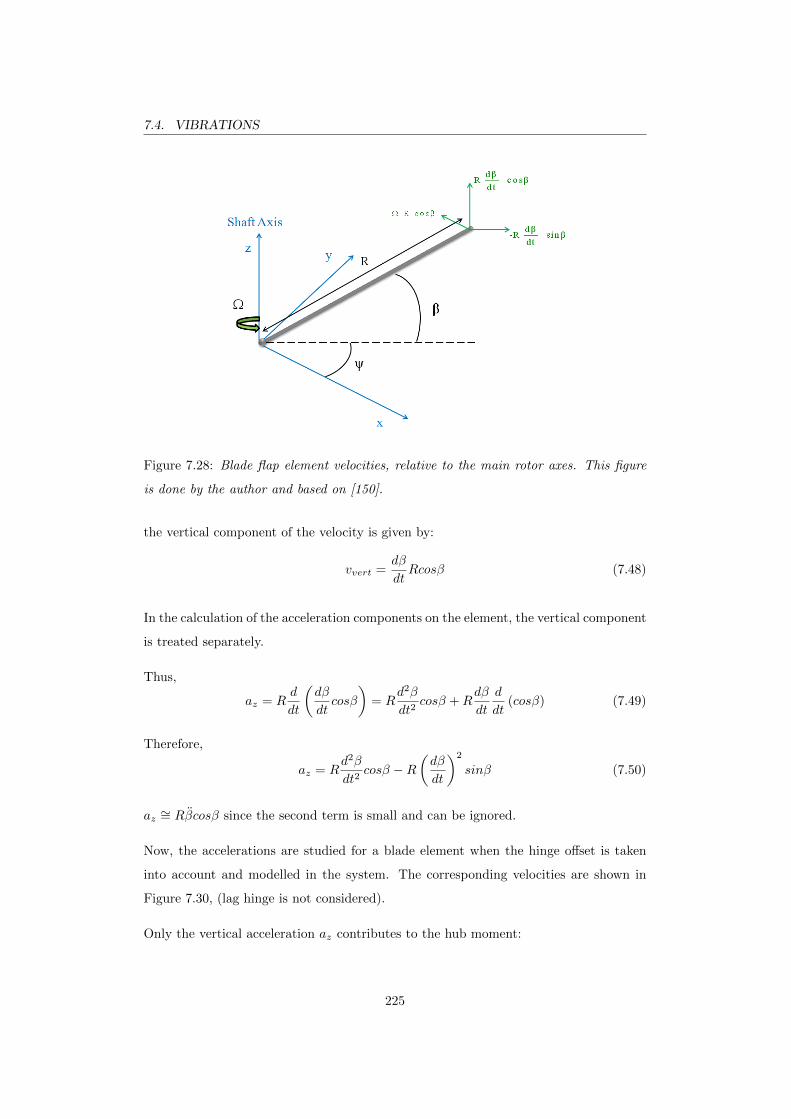
7.4. VIBRATIONS
Figure 7.28: Blade flap element velocities, relative to the main rotor axes. This figure
is done by the author and based on [150].
the vertical component of the velocity is given by:
vvert =dβ
dtRcosβ (7.48)
In the calculation of the acceleration components on the element, the vertical component
is treated separately.
Thus,
az = Rd
dt
(dβ
dtcosβ
)= R
d2β
dt2cosβ +R
dβ
dt
d
dt(cosβ) (7.49)
Therefore,
az = Rd2β
dt2cosβ −R
(dβ
dt
)2
sinβ (7.50)
az ∼= Rβcosβ since the second term is small and can be ignored.
Now, the accelerations are studied for a blade element when the hinge offset is taken
into account and modelled in the system. The corresponding velocities are shown in
Figure 7.30, (lag hinge is not considered).
Only the vertical acceleration az contributes to the hub moment:
225
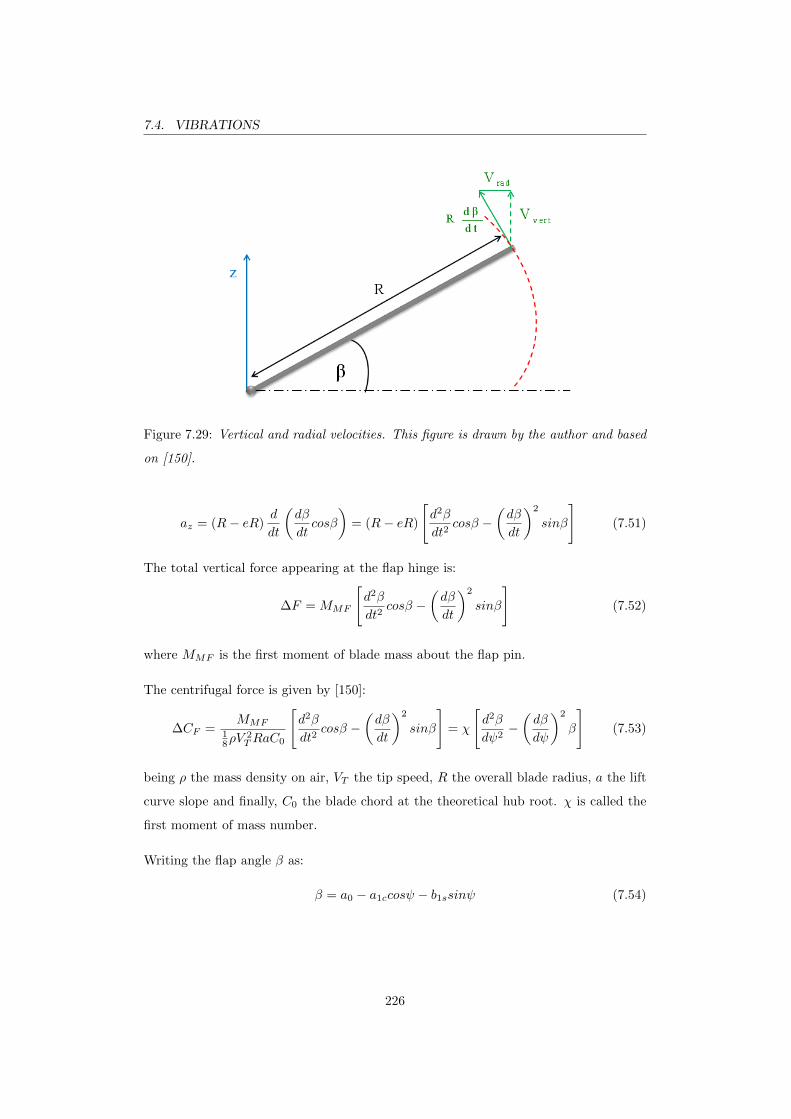
7.4. VIBRATIONS
Figure 7.29: Vertical and radial velocities. This figure is drawn by the author and based
on [150].
az = (R− eR)d
dt
(dβ
dtcosβ
)= (R− eR)
[d2β
dt2cosβ −
(dβ
dt
)2
sinβ
](7.51)
The total vertical force appearing at the flap hinge is:
∆F = MMF
[d2β
dt2cosβ −
(dβ
dt
)2
sinβ
](7.52)
where MMF is the first moment of blade mass about the flap pin.
The centrifugal force is given by [150]:
∆CF =MMF
18ρV
2TRaC0
[d2β
dt2cosβ −
(dβ
dt
)2
sinβ
]= χ
[d2β
dψ2−(dβ
dψ
)2
β
](7.53)
being ρ the mass density on air, VT the tip speed, R the overall blade radius, a the lift
curve slope and finally, C0 the blade chord at the theoretical hub root. χ is called the
first moment of mass number.
Writing the flap angle β as:
β = a0 − a1ccosψ − b1ssinψ (7.54)
226
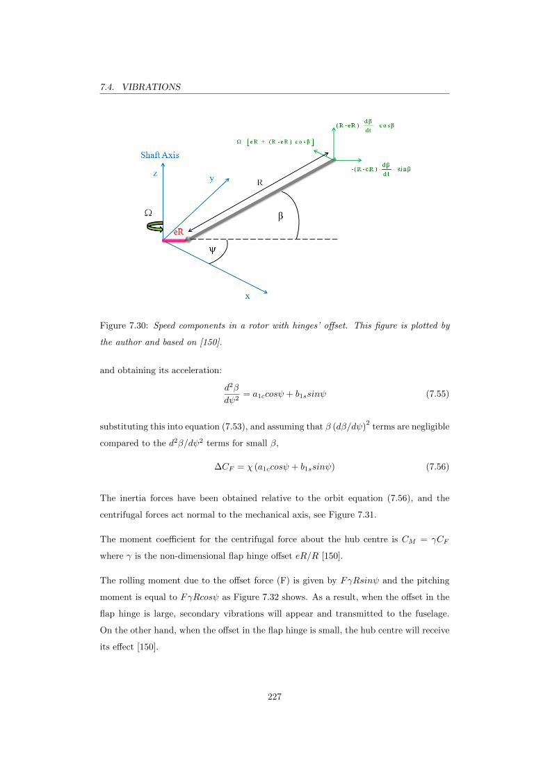
7.4. VIBRATIONS
Figure 7.30: Speed components in a rotor with hinges’ offset. This figure is plotted by
the author and based on [150].
and obtaining its acceleration:
d2β
dψ2= a1ccosψ + b1ssinψ (7.55)
substituting this into equation (7.53), and assuming that β (dβ/dψ)2
terms are negligible
compared to the d2β/dψ2 terms for small β,
∆CF = χ (a1ccosψ + b1ssinψ) (7.56)
The inertia forces have been obtained relative to the orbit equation (7.56), and the
centrifugal forces act normal to the mechanical axis, see Figure 7.31.
The moment coefficient for the centrifugal force about the hub centre is CM = γCF
where γ is the non-dimensional flap hinge offset eR/R [150].
The rolling moment due to the offset force (F) is given by FγRsinψ and the pitching
moment is equal to FγRcosψ as Figure 7.32 shows. As a result, when the offset in the
flap hinge is large, secondary vibrations will appear and transmitted to the fuselage.
On the other hand, when the offset in the flap hinge is small, the hub centre will receive
its effect [150].
227
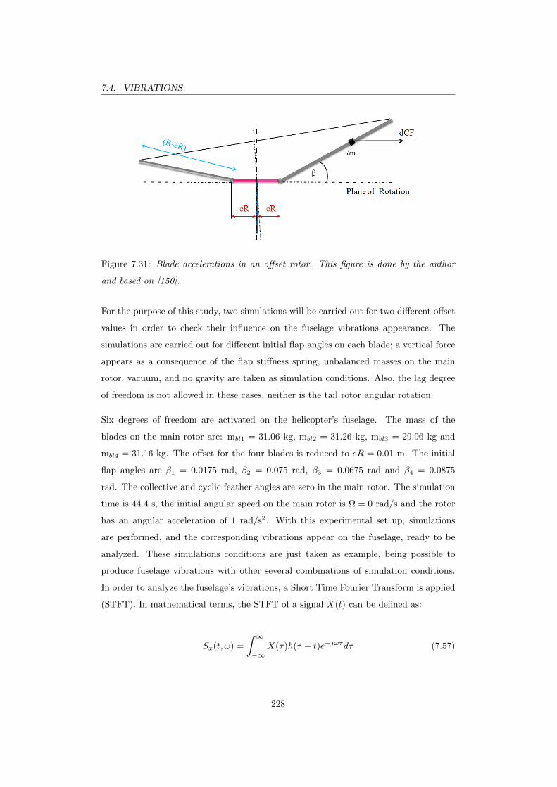
7.4. VIBRATIONS
Figure 7.31: Blade accelerations in an offset rotor. This figure is done by the author
and based on [150].
For the purpose of this study, two simulations will be carried out for two different offset
values in order to check their influence on the fuselage vibrations appearance. The
simulations are carried out for different initial flap angles on each blade; a vertical force
appears as a consequence of the flap stiffness spring, unbalanced masses on the main
rotor, vacuum, and no gravity are taken as simulation conditions. Also, the lag degree
of freedom is not allowed in these cases, neither is the tail rotor angular rotation.
Six degrees of freedom are activated on the helicopter’s fuselage. The mass of the
blades on the main rotor are: mbl1 = 31.06 kg, mbl2 = 31.26 kg, mbl3 = 29.96 kg and
mbl4 = 31.16 kg. The offset for the four blades is reduced to eR = 0.01 m. The initial
flap angles are β1 = 0.0175 rad, β2 = 0.075 rad, β3 = 0.0675 rad and β4 = 0.0875
rad. The collective and cyclic feather angles are zero in the main rotor. The simulation
time is 44.4 s, the initial angular speed on the main rotor is Ω = 0 rad/s and the rotor
has an angular acceleration of 1 rad/s2. With this experimental set up, simulations
are performed, and the corresponding vibrations appear on the fuselage, ready to be
analyzed. These simulations conditions are just taken as example, being possible to
produce fuselage vibrations with other several combinations of simulation conditions.
In order to analyze the fuselage’s vibrations, a Short Time Fourier Transform is applied
(STFT). In mathematical terms, the STFT of a signal X(t) can be defined as:
Sx(t, ω) =
∫ ∞−∞
X(τ)h(τ − t)e−jωτdτ (7.57)
228
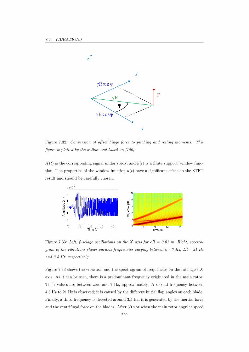
7.4. VIBRATIONS
Figure 7.32: Conversion of offset hinge force to pitching and rolling moments. This
figure is plotted by the author and based on [150].
X(t) is the corresponding signal under study, and h(t) is a finite support window func-
tion. The properties of the window function h(t) have a significant effect on the STFT
result and should be carefully chosen.
Figure 7.33: Left, fuselage oscillations on the X axis for eR = 0.01 m. Right, spectro-
gram of the vibrations shows various frequencies varying between 0 - 7 Hz, 4.5 - 21 Hz
and 3.5 Hz, respectively.
Figure 7.33 shows the vibration and the spectrogram of frequencies on the fuselage’s X
axis. As it can be seen, there is a predominant frequency originated in the main rotor.
Their values are between zero and 7 Hz, approximately. A second frequency between
4.5 Hz to 21 Hz is observed; it is caused by the different initial flap angles on each blade.
Finally, a third frequency is detected around 3.5 Hz, it is generated by the inertial force
and the centrifugal force on the blades. After 30 s or when the main rotor angular speed
229
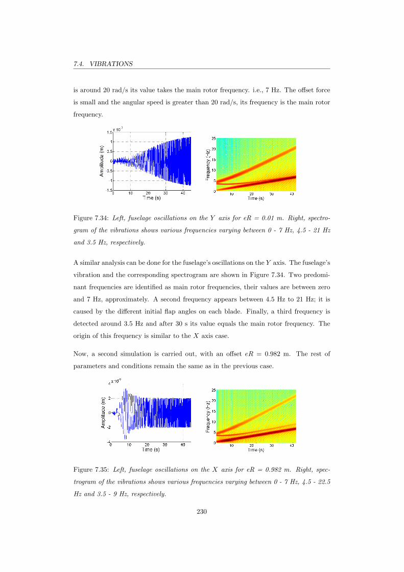
7.4. VIBRATIONS
is around 20 rad/s its value takes the main rotor frequency. i.e., 7 Hz. The offset force
is small and the angular speed is greater than 20 rad/s, its frequency is the main rotor
frequency.
Figure 7.34: Left, fuselage oscillations on the Y axis for eR = 0.01 m. Right, spectro-
gram of the vibrations shows various frequencies varying between 0 - 7 Hz, 4.5 - 21 Hz
and 3.5 Hz, respectively.
A similar analysis can be done for the fuselage’s oscillations on the Y axis. The fuselage’s
vibration and the corresponding spectrogram are shown in Figure 7.34. Two predomi-
nant frequencies are identified as main rotor frequencies, their values are between zero
and 7 Hz, approximately. A second frequency appears between 4.5 Hz to 21 Hz; it is
caused by the different initial flap angles on each blade. Finally, a third frequency is
detected around 3.5 Hz and after 30 s its value equals the main rotor frequency. The
origin of this frequency is similar to the X axis case.
Now, a second simulation is carried out, with an offset eR = 0.982 m. The rest of
parameters and conditions remain the same as in the previous case.
Figure 7.35: Left, fuselage oscillations on the X axis for eR = 0.982 m. Right, spec-
trogram of the vibrations shows various frequencies varying between 0 - 7 Hz, 4.5 - 22.5
Hz and 3.5 - 9 Hz, respectively.
230
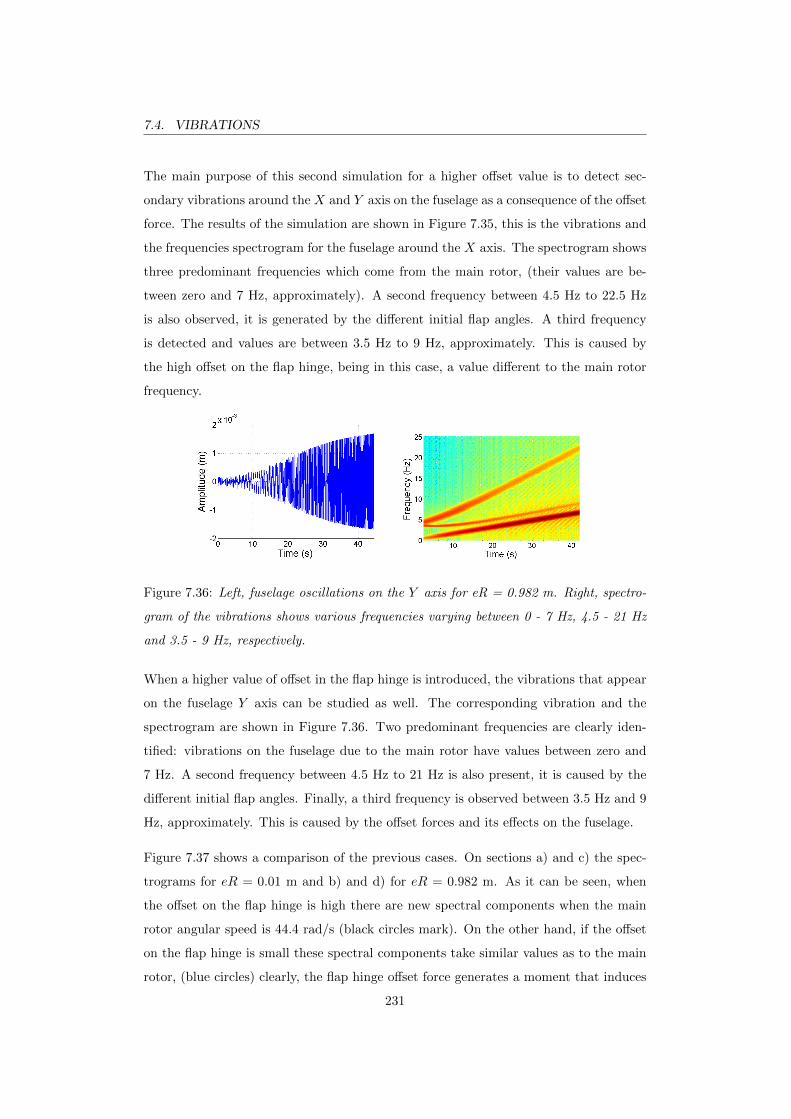
7.4. VIBRATIONS
The main purpose of this second simulation for a higher offset value is to detect sec-
ondary vibrations around the X and Y axis on the fuselage as a consequence of the offset
force. The results of the simulation are shown in Figure 7.35, this is the vibrations and
the frequencies spectrogram for the fuselage around the X axis. The spectrogram shows
three predominant frequencies which come from the main rotor, (their values are be-
tween zero and 7 Hz, approximately). A second frequency between 4.5 Hz to 22.5 Hz
is also observed, it is generated by the different initial flap angles. A third frequency
is detected and values are between 3.5 Hz to 9 Hz, approximately. This is caused by
the high offset on the flap hinge, being in this case, a value different to the main rotor
frequency.
Figure 7.36: Left, fuselage oscillations on the Y axis for eR = 0.982 m. Right, spectro-
gram of the vibrations shows various frequencies varying between 0 - 7 Hz, 4.5 - 21 Hz
and 3.5 - 9 Hz, respectively.
When a higher value of offset in the flap hinge is introduced, the vibrations that appear
on the fuselage Y axis can be studied as well. The corresponding vibration and the
spectrogram are shown in Figure 7.36. Two predominant frequencies are clearly iden-
tified: vibrations on the fuselage due to the main rotor have values between zero and
7 Hz. A second frequency between 4.5 Hz to 21 Hz is also present, it is caused by the
different initial flap angles. Finally, a third frequency is observed between 3.5 Hz and 9
Hz, approximately. This is caused by the offset forces and its effects on the fuselage.
Figure 7.37 shows a comparison of the previous cases. On sections a) and c) the spec-
trograms for eR = 0.01 m and b) and d) for eR = 0.982 m. As it can be seen, when
the offset on the flap hinge is high there are new spectral components when the main
rotor angular speed is 44.4 rad/s (black circles mark). On the other hand, if the offset
on the flap hinge is small these spectral components take similar values as to the main
rotor, (blue circles) clearly, the flap hinge offset force generates a moment that induces
231
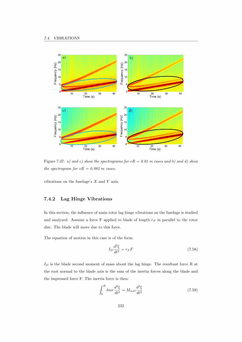
7.4. VIBRATIONS
Figure 7.37: a) and c) show the spectrograms for eR = 0.01 m cases and b) and d) show
the spectrogram for eR = 0.982 m cases.
vibrations on the fuselage’s X and Y axis.
7.4.2 Lag Hinge Vibrations
In this section, the influence of main rotor lag hinge vibrations on the fuselage is studied
and analyzed. Assume a force F applied to blade of length rF in parallel to the rotor
disc. The blade will move due to this force.
The equation of motion in this case is of the form:
IDd2ξ
dt2= rFF (7.58)
ID is the blade second moment of mass about the lag hinge. The resultant force R at
the root normal to the blade axis is the sum of the inertia forces along the blade and
the impressed force F. The inertia force is then:∫ R
0
δmrd2ξ
dt2= MmD
d2ξ
dt2(7.59)
232
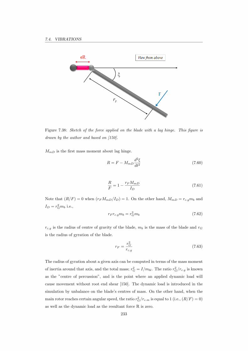
7.4. VIBRATIONS
Figure 7.38: Sketch of the force applied on the blade with a lag hinge. This figure is
drawn by the author and based on [150].
MmD is the first mass moment about lag hinge.
R = F −MmDd2ξ
dt2(7.60)
R
F= 1− rFMmD
ID(7.61)
Note that (R/F ) = 0 when (rFMmD/ID) = 1. On the other hand, MmD = rc.gmb and
ID = r2Gmb i.e.,
rF rc.gmb = r2Gmb (7.62)
rc.g is the radius of centre of gravity of the blade, mb is the mass of the blade and rG
is the radius of gyration of the blade.
rF =r2G
rc.g(7.63)
The radius of gyration about a given axis can be computed in terms of the mass moment
of inertia around that axis, and the total mass; r2G = I/mbl. The ratio r2
G/rc.g is known
as the ”centre of percussion”, and is the point where an applied dynamic load will
cause movement without root end shear [150]. The dynamic load is introduced in the
simulation by unbalance on the blade’s centres of mass. On the other hand, when the
main rotor reaches certain angular speed, the ratio r2G/rc.m is equal to 1 (i.e., (R/F ) = 0)
as well as the dynamic load as the resultant force R is zero.
233

7.4. VIBRATIONS
If the centre of mass of each blade is located at different points, this configuration will
introduce a dynamic load on the main rotor as well as vibrations on the fuselage. The
flap degree of freedom in this case is not modelled in order to study only lag hinge
originated vibrations.
The six degrees of freedom are allowed on the helicopter’s fuselage and the mass of the
blades on the main rotor and the tail are equally balanced. The centre of mass of the
four blades on the main rotor are unbalanced as ybl1 = 2.9846 m, ybl2 = 2.7846 m,
ybl3 = 2.8846 m and ybl4 = 2.6846 m. Collective and cyclic feather angles are zero in
the main rotor. The tail rotor angular rotation is deactivated. The simulation time is
44.4 s, the initial angular speed is zero and an acceleration of 1 rad/s2 is introduced
in the simulation. This configuration is enough to generate vibrations on the fuselage.
Several other combinations could be chosen. This particular one is provided as means
of illustration and validation of the model.
Figure 7.39: Left, fuselage oscillations on the X axis for ybl1 = 2.9846 m, ybl2 = 2.7846
m, ybl3 = 2.8846 m, ybl4 = 2.6846 m. Right, spectrogram of the vibrations shows various
frequencies varying between 0 - 7 Hz, 7 - 9 Hz, respectively.
From the spectrogram of frequencies shown in Figure 7.39, the signal on the fuselage’s
X axis is a predominant frequency which comes from the main rotor, its values are
between 0 and 7 Hz, approximately. As it can be seen, a second frequency is detected
around 7 Hz and 9 Hz, being its time interval 5 s, after this time, the signal disappears.
This frequency appears because during this time interval, the ratio (R/F ) 6= 0 and so
the applied dynamic load generates a force at the blade’s root axis and it is transmitted
to the fuselage in the form of vibration.
Similar analysis is carried out for vibrations appearing on the fuselage on the Y direction.
In Figure 7.40, a predominant frequency is observed between 0 and 7 Hz, it is originated
234
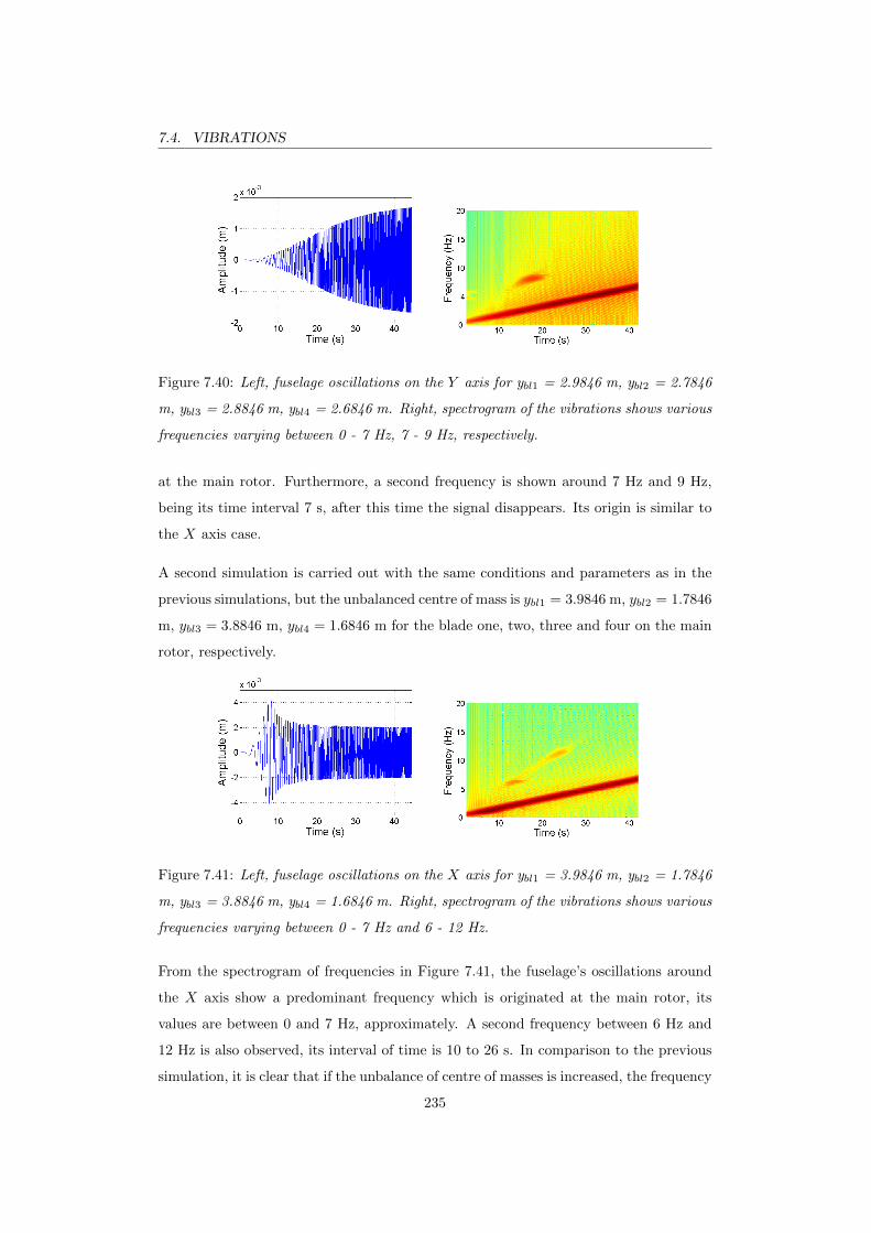
7.4. VIBRATIONS
Figure 7.40: Left, fuselage oscillations on the Y axis for ybl1 = 2.9846 m, ybl2 = 2.7846
m, ybl3 = 2.8846 m, ybl4 = 2.6846 m. Right, spectrogram of the vibrations shows various
frequencies varying between 0 - 7 Hz, 7 - 9 Hz, respectively.
at the main rotor. Furthermore, a second frequency is shown around 7 Hz and 9 Hz,
being its time interval 7 s, after this time the signal disappears. Its origin is similar to
the X axis case.
A second simulation is carried out with the same conditions and parameters as in the
previous simulations, but the unbalanced centre of mass is ybl1 = 3.9846 m, ybl2 = 1.7846
m, ybl3 = 3.8846 m, ybl4 = 1.6846 m for the blade one, two, three and four on the main
rotor, respectively.
Figure 7.41: Left, fuselage oscillations on the X axis for ybl1 = 3.9846 m, ybl2 = 1.7846
m, ybl3 = 3.8846 m, ybl4 = 1.6846 m. Right, spectrogram of the vibrations shows various
frequencies varying between 0 - 7 Hz and 6 - 12 Hz.
From the spectrogram of frequencies in Figure 7.41, the fuselage’s oscillations around
the X axis show a predominant frequency which is originated at the main rotor, its
values are between 0 and 7 Hz, approximately. A second frequency between 6 Hz and
12 Hz is also observed, its interval of time is 10 to 26 s. In comparison to the previous
simulation, it is clear that if the unbalance of centre of masses is increased, the frequency
235
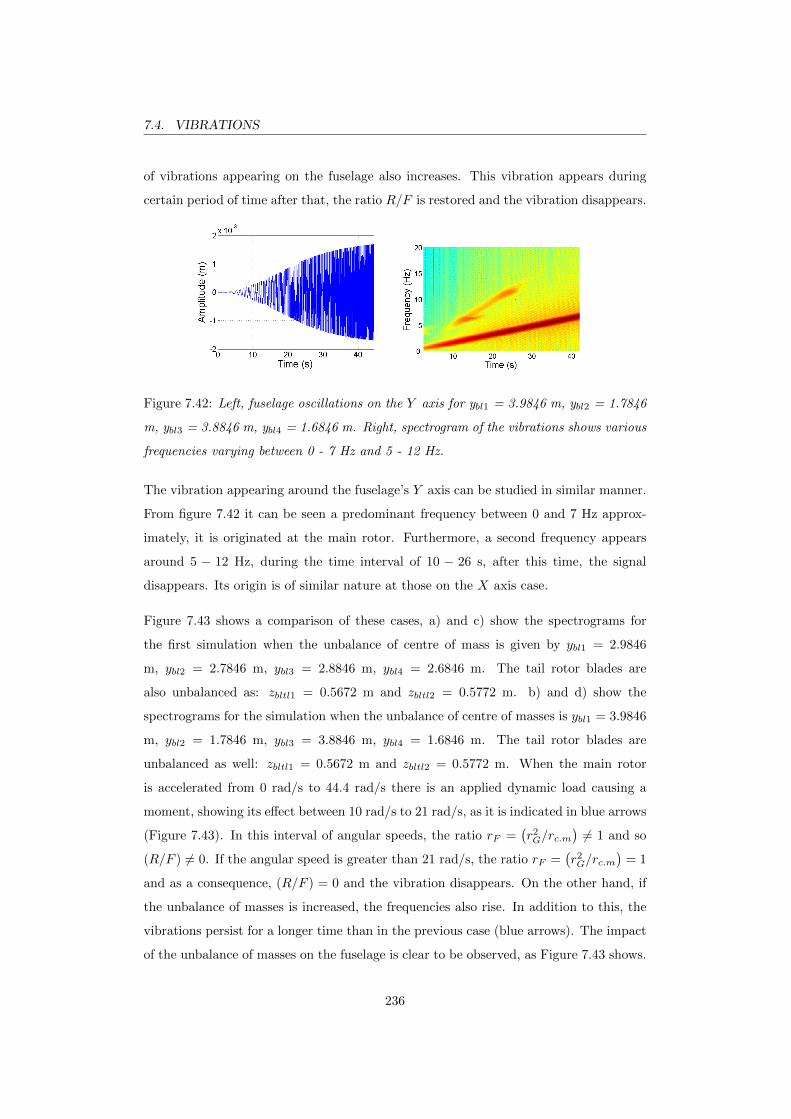
7.4. VIBRATIONS
of vibrations appearing on the fuselage also increases. This vibration appears during
certain period of time after that, the ratio R/F is restored and the vibration disappears.
Figure 7.42: Left, fuselage oscillations on the Y axis for ybl1 = 3.9846 m, ybl2 = 1.7846
m, ybl3 = 3.8846 m, ybl4 = 1.6846 m. Right, spectrogram of the vibrations shows various
frequencies varying between 0 - 7 Hz and 5 - 12 Hz.
The vibration appearing around the fuselage’s Y axis can be studied in similar manner.
From figure 7.42 it can be seen a predominant frequency between 0 and 7 Hz approx-
imately, it is originated at the main rotor. Furthermore, a second frequency appears
around 5 − 12 Hz, during the time interval of 10 − 26 s, after this time, the signal
disappears. Its origin is of similar nature at those on the X axis case.
Figure 7.43 shows a comparison of these cases, a) and c) show the spectrograms for
the first simulation when the unbalance of centre of mass is given by ybl1 = 2.9846
m, ybl2 = 2.7846 m, ybl3 = 2.8846 m, ybl4 = 2.6846 m. The tail rotor blades are
also unbalanced as: zbltl1 = 0.5672 m and zbltl2 = 0.5772 m. b) and d) show the
spectrograms for the simulation when the unbalance of centre of masses is ybl1 = 3.9846
m, ybl2 = 1.7846 m, ybl3 = 3.8846 m, ybl4 = 1.6846 m. The tail rotor blades are
unbalanced as well: zbltl1 = 0.5672 m and zbltl2 = 0.5772 m. When the main rotor
is accelerated from 0 rad/s to 44.4 rad/s there is an applied dynamic load causing a
moment, showing its effect between 10 rad/s to 21 rad/s, as it is indicated in blue arrows
(Figure 7.43). In this interval of angular speeds, the ratio rF =(r2G/rc.m
)6= 1 and so
(R/F ) 6= 0. If the angular speed is greater than 21 rad/s, the ratio rF =(r2G/rc.m
)= 1
and as a consequence, (R/F ) = 0 and the vibration disappears. On the other hand, if
the unbalance of masses is increased, the frequencies also rise. In addition to this, the
vibrations persist for a longer time than in the previous case (blue arrows). The impact
of the unbalance of masses on the fuselage is clear to be observed, as Figure 7.43 shows.
236
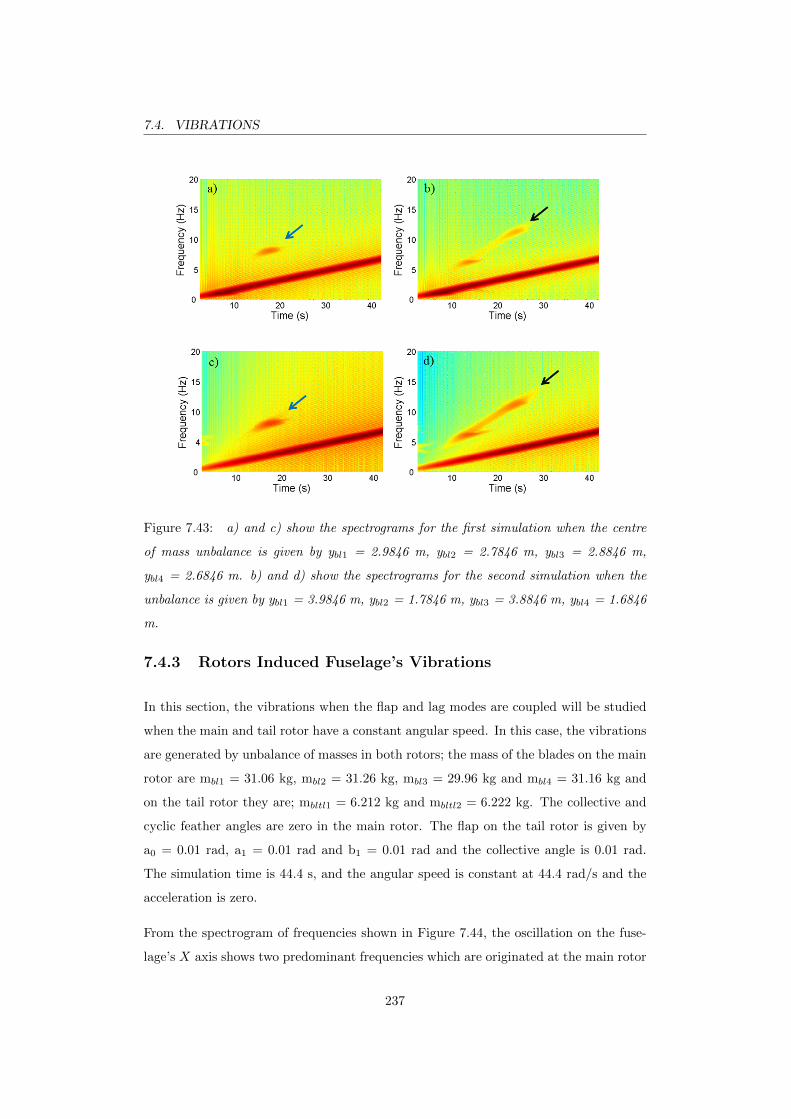
7.4. VIBRATIONS
Figure 7.43: a) and c) show the spectrograms for the first simulation when the centre
of mass unbalance is given by ybl1 = 2.9846 m, ybl2 = 2.7846 m, ybl3 = 2.8846 m,
ybl4 = 2.6846 m. b) and d) show the spectrograms for the second simulation when the
unbalance is given by ybl1 = 3.9846 m, ybl2 = 1.7846 m, ybl3 = 3.8846 m, ybl4 = 1.6846
m.
7.4.3 Rotors Induced Fuselage’s Vibrations
In this section, the vibrations when the flap and lag modes are coupled will be studied
when the main and tail rotor have a constant angular speed. In this case, the vibrations
are generated by unbalance of masses in both rotors; the mass of the blades on the main
rotor are mbl1 = 31.06 kg, mbl2 = 31.26 kg, mbl3 = 29.96 kg and mbl4 = 31.16 kg and
on the tail rotor they are; mbltl1 = 6.212 kg and mbltl2 = 6.222 kg. The collective and
cyclic feather angles are zero in the main rotor. The flap on the tail rotor is given by
a0 = 0.01 rad, a1 = 0.01 rad and b1 = 0.01 rad and the collective angle is 0.01 rad.
The simulation time is 44.4 s, and the angular speed is constant at 44.4 rad/s and the
acceleration is zero.
From the spectrogram of frequencies shown in Figure 7.44, the oscillation on the fuse-
lage’s X axis shows two predominant frequencies which are originated at the main rotor
237
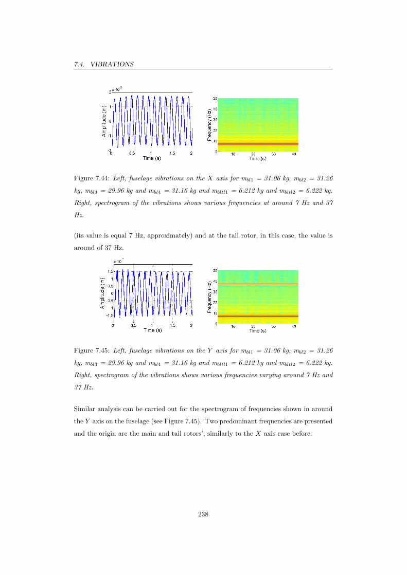
7.4. VIBRATIONS
Figure 7.44: Left, fuselage vibrations on the X axis for mbl1 = 31.06 kg, mbl2 = 31.26
kg, mbl3 = 29.96 kg and mbl4 = 31.16 kg and mbltl1 = 6.212 kg and mbltl2 = 6.222 kg.
Right, spectrogram of the vibrations shows various frequencies at around 7 Hz and 37
Hz.
(its value is equal 7 Hz, approximately) and at the tail rotor, in this case, the value is
around of 37 Hz.
Figure 7.45: Left, fuselage vibrations on the Y axis for mbl1 = 31.06 kg, mbl2 = 31.26
kg, mbl3 = 29.96 kg and mbl4 = 31.16 kg and mbltl1 = 6.212 kg and mbltl2 = 6.222 kg.
Right, spectrogram of the vibrations shows various frequencies varying around 7 Hz and
37 Hz.
Similar analysis can be carried out for the spectrogram of frequencies shown in around
the Y axis on the fuselage (see Figure 7.45). Two predominant frequencies are presented
and the origin are the main and tail rotors’, similarly to the X axis case before.
238
7.5. CHAPTER SUMMARY
7.5 Chapter Summary
The aim of this chapter is to demonstrate that the dynamical model built in VehicleSim
behaviour coincides with that predicted by the theory. VehicleSim can be regarded as
typical symbolic mechanical multibody modelling software, which writes ready-to-run
simulation code. In fact, the linear and nonlinear equations for flap, lag and coupled
flap-lag motions as well as feather motion have been obtained and validated.
In the present study, the effects of various values of blade offset, springs stiffness and
damping coefficients fitted on the blades’ hinges were studied for the flap and lag cases, in
order to present a dynamic model of blade’s motion. In these cases, the obtained results
have proven to be correct by theory validation. As is the case with many nonlinear
systems, the study of complex phenomenon on the dynamic structures is investigated
via the eigenvalues of linearised models that are associated to the equilibrium of the
nonlinear system. VehicleSim is used to generate the time histories of the nonlinear
equations of motion and it also derives the linearised state-space models. The nonlinear
equations are stored into two files with extensions .erd and .bin, the linearised equations
of motion are stored as a Matlab file and the root locus was obtained to study the
stability of the flap, lag as well as the fuselage.
The coupled vertical movement between the fuselage and the flap degree of freedom was
studied. Several modes of oscillations were analyzed via eigenvalues and eigenvectors
analysis. The influence of the mass ratio massblade/massfuselage on the coupled modes
has been demonstrated. The influence of the fuselage on the flap motion was also
analyzed and studied as a consequence of the gyroscopic effect on the fuselage.
It is worth recalling that two studies showed a coupling between the fuselage and the flap
degree of freedom. A third study was performed in order to analyze the influence of the
lag degree of freedom on the fuselage. The simulations carried out in this chapter using
the VehicleSim model showed good agreement with the theoretical findings existing in
the literature.
The tail rotor and the effect of the delta three angles have also been studied for various
cases. It was shown how the flap frequencies increased as a function of the advance
ratio as a consequence of the delta three angle coupling. Furthermore, maximum flap
amplitude and feather angle decrease was shown as a result of the existing positive
239
7.5. CHAPTER SUMMARY
coupling.
The control of the six degrees of freedom of the helicopter has been implemented in the
model by using PID controllers. This procedure was a priority task (in order to maintain
the equilibrium on the system). The control action was shown for the translational and
the rotational degrees of freedom, providing the system with the required equilibrium
around the initial position. Additionally, the ratio between the angular speed on the
main and tail rotors was modelled with immediate response, this ratio was achieved
when both rotor were accelerated, being possible to simulate a delay on the rotors as
a consequence of the engine response. On the other hand, the vibrations originated at
the rotors were simulated and their effects on the fuselage were studied. Three different
cases were analyzed and presented and in all of them, a clear impact of these vibrations
into the fuselage was shown.
In conclusion, a comprehensive dynamical study for a helicopter with Sikorsky config-
uration was presented. The simulations were designed for different cases in order to
validate the helicopter model obtained. The tests carried out proved the correct imple-
mentation of the model and its readiness to be used in future works for further modelling
or control systems implementation purposes.
240
Chapter 8
Sikorsky Model in Presence of
External Perturbations
The purpose of this chapter is to study the aerodynamic environment together with
gravity on the helicopter as well as to study the effect the main rotor inclination has
on the helicopter when aerodynamic forces are considered. As mentioned in previous
chapters, vibrations play a relevant role in helicopter’s performance. The effects are
individually analyzed by assuming that the helicopter’s nominal configuration is as
described in Chapter 6. The analysis is carried out purely through simulations. The
equations of motion are obtained for the cases of flap, lift, lag and drag forces. An
aerodynamic analysis is carried out for a six degrees of freedom fuselage, a three degrees
of freedom (flap, lag and feather) main rotor blades and flap-feather on the tail rotor
coupling. Blade elements are modelled on the main and tail rotors to simulate the
flight conditions of hover, climb, descent and forward flight. Each one of these flight
conditions is simulated and the results are shown. After that, different trajectories are
represented in forward flight, as well as combinations of several flight conditions so that
the model can describe trajectories in a satisfactory manner. In addition to this, the
drift effect is also considered and analyzed. The vibrations as a consequence of the
varying rotating main rotor speed are carefully studied, they are analyzed in absence of
aerodynamic forces. Finally, the impact of vibrations in hover flight is studied on the
fuselage.
241
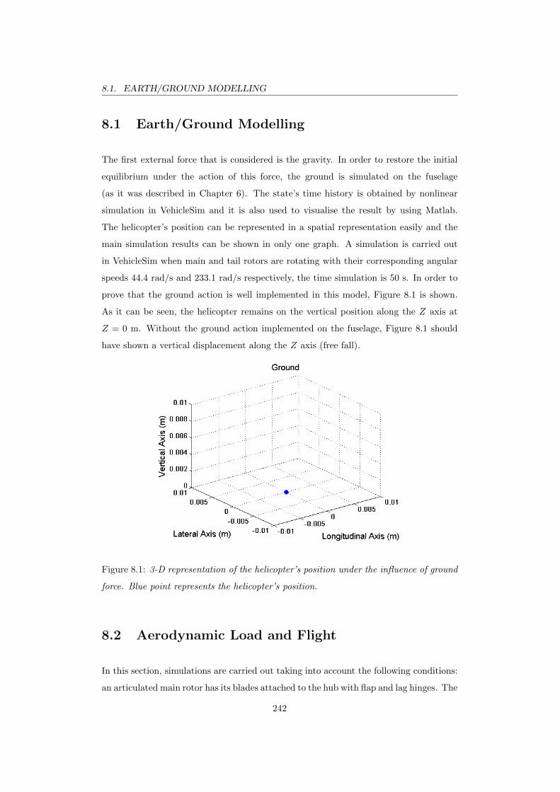
8.1. EARTH/GROUND MODELLING
8.1 Earth/Ground Modelling
The first external force that is considered is the gravity. In order to restore the initial
equilibrium under the action of this force, the ground is simulated on the fuselage
(as it was described in Chapter 6). The state’s time history is obtained by nonlinear
simulation in VehicleSim and it is also used to visualise the result by using Matlab.
The helicopter’s position can be represented in a spatial representation easily and the
main simulation results can be shown in only one graph. A simulation is carried out
in VehicleSim when main and tail rotors are rotating with their corresponding angular
speeds 44.4 rad/s and 233.1 rad/s respectively, the time simulation is 50 s. In order to
prove that the ground action is well implemented in this model, Figure 8.1 is shown.
As it can be seen, the helicopter remains on the vertical position along the Z axis at
Z = 0 m. Without the ground action implemented on the fuselage, Figure 8.1 should
have shown a vertical displacement along the Z axis (free fall).
Figure 8.1: 3-D representation of the helicopter’s position under the influence of ground
force. Blue point represents the helicopter’s position.
8.2 Aerodynamic Load and Flight
In this section, simulations are carried out taking into account the following conditions:
an articulated main rotor has its blades attached to the hub with flap and lag hinges. The
242
8.2. AERODYNAMIC LOAD AND FLIGHT
flap hinge is usually offset from the centre of rotation because of mechanical constraints
and to improve the helicopter handling qualities. The lag hinge must be offset in order
for the shaft to transmit torque to the rotor. The purpose of the flap and lag hinges is
to reduce the root blade loads. With a lag hinge, a mechanical lag damper to avoid a
mechanical instability called ground resonance is needed [140]. As a consequence, the
springs on the flap and lag hinges included in the dynamical model are not needed as
the restoring moments are provided by the aerodynamic forces, the lag damper remains.
8.2.1 Aerodynamic Load Equations
The nonlinear equations of motion for the aerodynamic model can be obtained from
VehicleSim. In order to validate these, they will be compared to those predicted by
theoretical studies. The results for the case of uncoupled flap and lag degrees of freedom
are presented in here. It is convenient to bear in mind that the case under study is for
rigid blades, being flexibility and torsion two effects not considered in this work. The
aerodynamic equations are obtained for one blade in hover flight conditions and the
main rotor angular speed is given by restriction in order to obtain simpler equations.
The corresponding aerodynamic forces are applied to the point xa = 0.0675 m being
this the coordinate of the blade’s centre of pressure i.e., 3/4 chord [98]. The distance
along the Y axis on the blades is ya = 3.24 m.
Flap Equation with Aerodynamical Load Validation
Flap is the first degree of freedom on the main rotor blade under the influence of the
aerodynamic forces to be studied. A restoring moment is provided by the lift force and
this induces flap. As a result, a vertical force appears on the helicopter, a flap offset
is also considered. Taking all these into account the equations of motion are obtained
after a simulation is run.
As it was mentioned in Chapter 7, one of the most comprehensive surveys on rotor
dynamics is proposed by [141], where the flap motion was represented by a second order
differential equation of the form:
243

8.2. AERODYNAMIC LOAD AND FLIGHT
Bβ + Ω2(Bcosβ +MbexgR
2)sinβ = MA (8.1)
where B is the moment of the inertia around the flap axis and MA is the aerodynamic
moment and Mb is the blade mass. In here, the position vector of the blade’s c.g (centre
of gravity) is rg = xgR. In our system, the blade’s centre of gravity is considered to lie
on the longitudinal axis, so it can be written as rg = yg. The equations are obtained
with the term eR instead of eR2, as it was explained in Chapter 7.
With the model provided including the aerodynamical load, a simulation is carried out
in VehicleSim. The software provides the nonlinear equation of motion corresponding
to the dynamic and aerodynamic loads and the rotor’s provided geometry. Equation
(8.2) is the aerodynamic equation for a blade with flap degree of freedom and it can be
validated by comparing it to equation (8.1).
β(Iblx +mbl · y2
bl
)+ Ω2 · (((Iblz − Ibly) +mbl · y2
bl) · cosβ + (mbl · eR · ybl)) · sinβ
= dya · 12 · Ω
2 · ρ · chord · (−(−2 · π · xa · (y2a + eR2) · sin(2 · π · qbl)− 2 · π · (cos(2·
π · qbl) · (y3a + eR3 · cos(2 · π · qbl)) + eR3 · sin(2 · π · qbl)2) + eR · (ya · (−4 · π · xa·
sin(2 · π · qbl) + eR · (4 · π − 4 · π · cos(2 · π · qbl)2) + ya · (2 · π − cos(2 · π · qbl) · (4·
π + 2 · π · cos(2 · π · qbl))− 2 · π · sin(2 · π · qbl)2)) + eR · (2 · π · eR− ya · (2 · π · cos
(2 · π · qbl) + 4 · π · sin(2 · π · qbl)2)))) · atan(vih/Ω · (ya + eR)))
(8.2)
qbl = (nblades− blade number1)/nblades, ρ is the air density, chord is the chord of the
blade, dya is the length differential interval, and vih is the hover induced velocity.
If a comparison between equations (8.1) and (8.2) is performed (although (8.2) is a more
extensive equation), similarities between both can be found:
• Bβ ∼=(Iblx +mbl · y2
bl
)β
• Ω2(Bcosβ +MbexgR
2)sinβ ∼=
Ω2 · (((Iblz − Ibly) +mbl · y2bl) · cosβ + (mbl · eR · ybl)) · sinβ
• MA is equal to the terms on the right hand side in equations (8.2)
Taking into account the previous considerations about the centre of gravity, after some
simplifications, both equations (8.1) and (8.2) are shown to be equal.
244
8.2. AERODYNAMIC LOAD AND FLIGHT
Lag Equation with Aerodynamical Load Validation
The nonlinear lag aerodynamic equation can be obtained in a similar way using Ve-
hicleSim. It is compared to those available in the literature. In order to validate the
equations obtained by VehicleSim, the following accepted expression for pure lag motion
is considered [141]:
Cξ +MbexgΩ2R2sinξ = N (8.3)
C is the moment of the inertia about the lag axis, N is the aerodynamic lag moment
and Mb is the blade mass.
Equation (8.4) is the aerodynamic equation for a blade with lag, in order to validate it,
it is compared to expression (8.3).
ξ(Iblz +mbl · y2bl) + Ω2 · eR ·mbl · ybl · sinξ = dya · 1
2 · Ω2 · ρ · chord · (−xa · sin(2 · π·
qbl) · (eR · (2 · ya · (δ0) + eR · (δ0)) + ya · (ya · (δ0)− atan(vih/Ω · (ya + eR)) · (ya · (δ1+δ2 · (−atan(vih/Ω · (ya + eR)))) + eR · (2 · δ1 + δ2 · (−2 · atan(vih/Ω · (ya + eR)))))
)) + eR · (eR · (ya · (2 · δ0 − 2 · (δ0) · sin(2 · π · qbl)2 + 2 · atan(vih/Ω · (ya + eR)) · (δ1·sin(2 · π · qbl)2 + δ2 · atan(vih/Ω · (ya + eR)))) + xa · sin(2 · π · qbl) · atan(vih/Ω · (ya+eR)) · (δ1 + δ2 · (−atan(vih/Ω · (ya + eR)))) + eR · (δ0 − sin(2 · π · qbl)2 · (δ0))) + ya
·(−eR · (atan(vih/Ω · (ya + eR)) · (2 · δ1 + δ2 · (2 · sin(2 · π · qbl)2 · atan(vih/Ω · (ya+
eR))))) + ya · (δ0 − atan(vih/Ω · (ya + eR)) · (δ1 · cos(2 · π · qbl)2 + δ2 · (−cos(2 · π·
qbl)2 · atan(vih/Ω · (ya + eR))))− sin(2 · π · qbl)2 · (δ0))))− cos(2 · π · qbl) · (ya · (eR2
·(2 · (δ0) · cos(2 · π · qbl) + δ2 · (atan(vih/Ω · (ya + eR))2)) + ya · (ya · (δ0 − atan(vih
/Ω · (ya + eR)) · (δ1 + δ2 · (−atan(vih/Ω · (ya + eR))))) + eR · (2 · δ0 + atan(vih/Ω·
(ya + eR)) · (−2 · δ1 − δ2 · (−2 · atan(vih/Ω · (ya + eR))))))) + eR · (ya · eR · (δ0−
atan(vih/Ω · (ya + eR)) · (δ1 · (1 + 2 · cos(2 · π · qbl)) + δ2 · (−2 · cos(2 · π · qbl)·
atan(vih/Ω · (ya + eR))))) + cos(2 · π · qbl) · (eR2 · (δ0) + y2a · (δ0 − atan(vih/Ω·
(ya + eR)) · (δ1 + δ2 · (−atan(vih/Ω · (ya + eR)))))))))
(8.4)
qbl = (nblades−blade number1)/nblades, ρ is the air density, chord is the blade’s chord,
dya is the length differential interval, vih is the induced velocity in hover and δ0, δ1 and
δ2 are the corresponding drag coefficients values.
A term by term comparison between equation (8.3) (theory prediction) and equation
(8.4) is carried out:
245
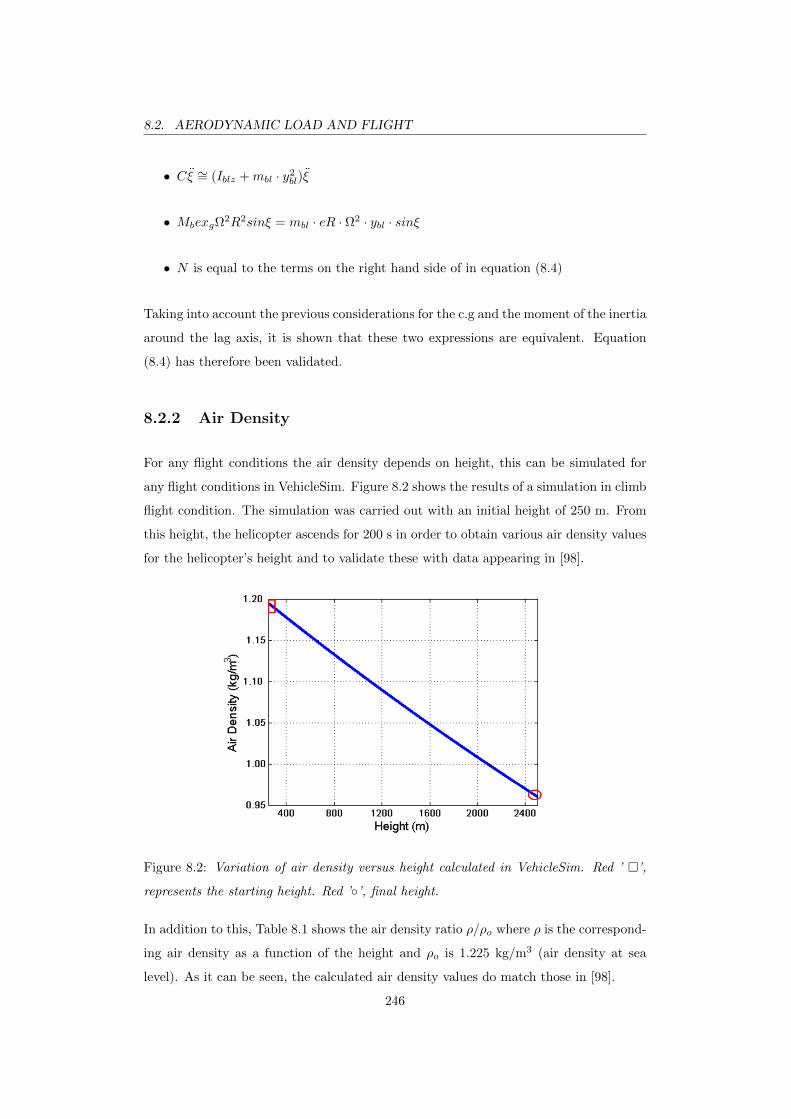
8.2. AERODYNAMIC LOAD AND FLIGHT
• Cξ ∼= (Iblz +mbl · y2bl)ξ
• MbexgΩ2R2sinξ = mbl · eR · Ω2 · ybl · sinξ
• N is equal to the terms on the right hand side of in equation (8.4)
Taking into account the previous considerations for the c.g and the moment of the inertia
around the lag axis, it is shown that these two expressions are equivalent. Equation
(8.4) has therefore been validated.
8.2.2 Air Density
For any flight conditions the air density depends on height, this can be simulated for
any flight conditions in VehicleSim. Figure 8.2 shows the results of a simulation in climb
flight condition. The simulation was carried out with an initial height of 250 m. From
this height, the helicopter ascends for 200 s in order to obtain various air density values
for the helicopter’s height and to validate these with data appearing in [98].
Figure 8.2: Variation of air density versus height calculated in VehicleSim. Red ’ ’,
represents the starting height. Red ’’, final height.
In addition to this, Table 8.1 shows the air density ratio ρ/ρo where ρ is the correspond-
ing air density as a function of the height and ρo is 1.225 kg/m3 (air density at sea
level). As it can be seen, the calculated air density values do match those in [98].
246
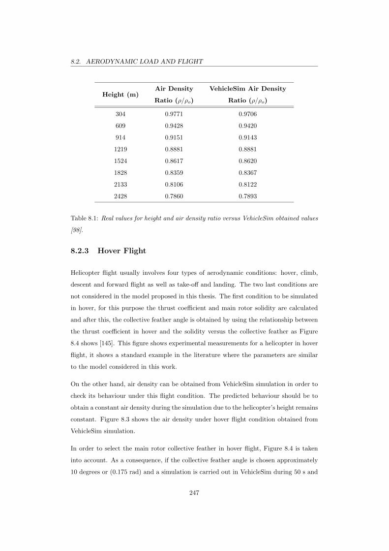
8.2. AERODYNAMIC LOAD AND FLIGHT
Height (m)Air Density
Ratio (ρ/ρo)
VehicleSim Air Density
Ratio (ρ/ρo)
304 0.9771 0.9706
609 0.9428 0.9420
914 0.9151 0.9143
1219 0.8881 0.8881
1524 0.8617 0.8620
1828 0.8359 0.8367
2133 0.8106 0.8122
2428 0.7860 0.7893
Table 8.1: Real values for height and air density ratio versus VehicleSim obtained values
[98].
8.2.3 Hover Flight
Helicopter flight usually involves four types of aerodynamic conditions: hover, climb,
descent and forward flight as well as take-off and landing. The two last conditions are
not considered in the model proposed in this thesis. The first condition to be simulated
in hover, for this purpose the thrust coefficient and main rotor solidity are calculated
and after this, the collective feather angle is obtained by using the relationship between
the thrust coefficient in hover and the solidity versus the collective feather as Figure
8.4 shows [145]. This figure shows experimental measurements for a helicopter in hover
flight, it shows a standard example in the literature where the parameters are similar
to the model considered in this work.
On the other hand, air density can be obtained from VehicleSim simulation in order to
check its behaviour under this flight condition. The predicted behaviour should be to
obtain a constant air density during the simulation due to the helicopter’s height remains
constant. Figure 8.3 shows the air density under hover flight condition obtained from
VehicleSim simulation.
In order to select the main rotor collective feather in hover flight, Figure 8.4 is taken
into account. As a consequence, if the collective feather angle is chosen approximately
10 degrees or (0.175 rad) and a simulation is carried out in VehicleSim during 50 s and
247
8.2. AERODYNAMIC LOAD AND FLIGHT
Figure 8.3: Air density in hover flight.
the helicopter’s height is 250 m, VehicleSim provides the parameter CT /σ = 0.099. So,
the main rotor feather angle as well as CT /σ match the expected ratio according to
Figure 8.4. The induced velocity in hover is given by vi0 =√T/2ρπR2.
On the other hand, the thrust coefficient and the solidity are also calculated for the
tail rotor. This allows to obtain the tail rotor collective feather angle in hover by using
the information provided in Figure 8.5 [71]. The collective angle is given for θ0.75 i.e.,
collective angle calculated at 75% of the radius of rotor. Nevertheless, the blades on
the tail rotor are rigid and without twist, so the feather angle is constant along the
blade length and this graph can be only used as an estimation to obtain the tail rotor
collective feather.
Once the main rotor feather angles is chosen, the tail rotor collective feather is selected
as approximately 10 degrees or (0.175 rad) in order to calculate CTtl/σtl, a simulation is
carried out for 50 seconds at h = 250 m and value obtained is CTtl/σtl = 0.045. Given
that, the tail rotor feather angle and CTtl/σtl keep the expected ratio according to Fig-
ure 8.5. These values for the tail collective feather together with main rotor collective
angle allow to simulate hover flight conditions. The yaw does not change, the helicopter
keeps the initial orientation around Z axis. Finally, hover conditions are simulated at a
height of 250 m. From h = 0 m to h = 250 m a climb flight takes place.
248
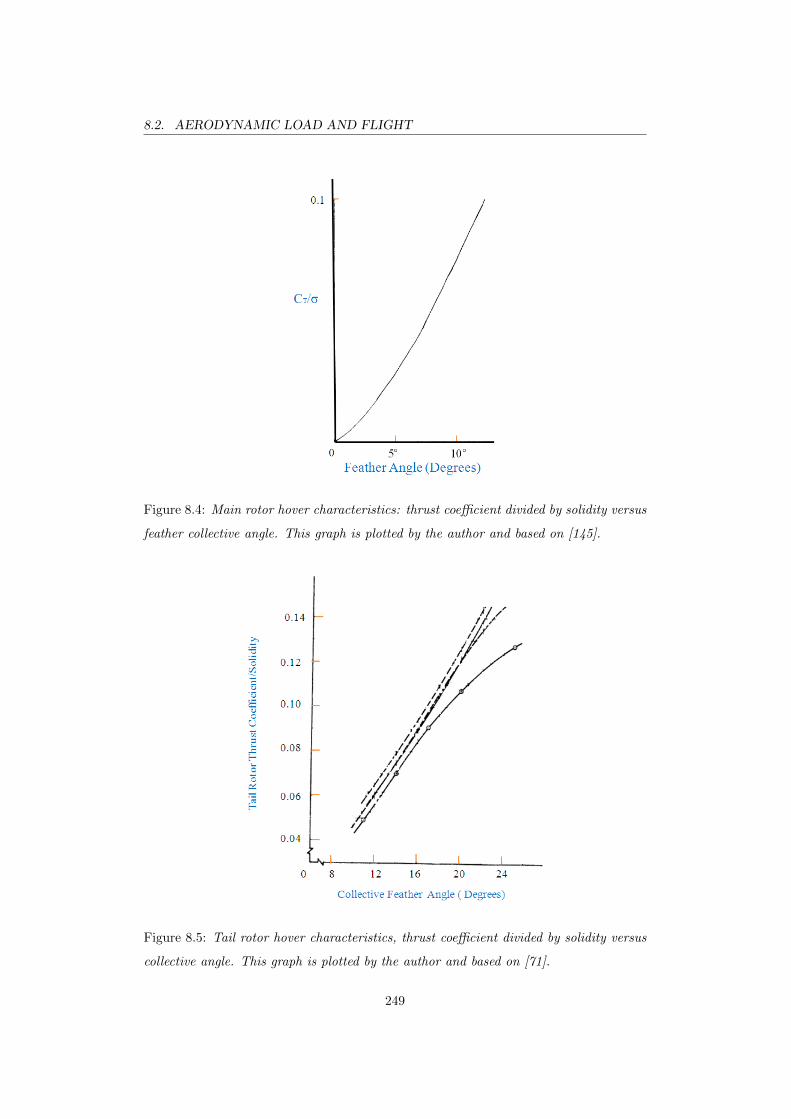
8.2. AERODYNAMIC LOAD AND FLIGHT
Figure 8.4: Main rotor hover characteristics: thrust coefficient divided by solidity versus
feather collective angle. This graph is plotted by the author and based on [145].
Figure 8.5: Tail rotor hover characteristics, thrust coefficient divided by solidity versus
collective angle. This graph is plotted by the author and based on [71].
249
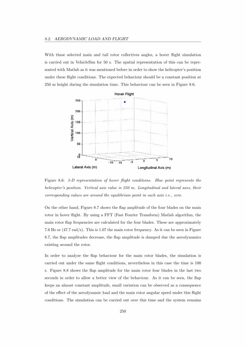
8.2. AERODYNAMIC LOAD AND FLIGHT
With these selected main and tail rotor collectives angles, a hover flight simulation
is carried out in VehicleSim for 50 s. The spatial representation of this can be repre-
sented with Matlab as it was mentioned before in order to show the helicopter’s position
under these flight conditions. The expected behaviour should be a constant position at
250 m height during the simulation time. This behaviour can be seen in Figure 8.6.
Figure 8.6: 3-D representation of hover flight conditions. Blue point represents the
helicopter’s position. Vertical axis value is 250 m. Longitudinal and lateral axes, their
corresponding values are around the equilibrium point in each axis i.e., zero.
On the other hand, Figure 8.7 shows the flap amplitude of the four blades on the main
rotor in hover flight. By using a FFT (Fast Fourier Transform) Matlab algorithm, the
main rotor flap frequencies are calculated for the four blades. These are approximately
7.6 Hz or (47.7 rad/s). This is 1.07 the main rotor frequency. As it can be seen in Figure
8.7, the flap amplitudes decrease, the flap amplitude is damped due the aerodynamics
existing around the rotor.
In order to analyze the flap behaviour for the main rotor blades, the simulation is
carried out under the same flight conditions, nevertheless in this case the time is 100
s. Figure 8.8 shows the flap amplitude for the main rotor four blades in the last two
seconds in order to allow a better view of the behaviour. As it can be seen, the flap
keeps an almost constant amplitude, small variation can be observed as a consequence
of the effect of the aerodynamic load and the main rotor angular speed under this flight
conditions. The simulation can be carried out over this time and the system remains
250
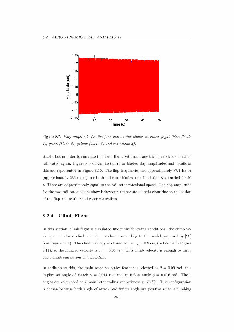
8.2. AERODYNAMIC LOAD AND FLIGHT
Figure 8.7: Flap amplitude for the four main rotor blades in hover flight (blue (blade
1), green (blade 2), yellow (blade 3) and red (blade 4)).
stable, but in order to simulate the hover flight with accuracy the controllers should be
calibrated again. Figure 8.9 shows the tail rotor blades’ flap amplitudes and details of
this are represented in Figure 8.10. The flap frequencies are approximately 37.1 Hz or
(approximately 233 rad/s), for both tail rotor blades, the simulation was carried for 50
s. These are approximately equal to the tail rotor rotational speed. The flap amplitude
for the two tail rotor blades show behaviour a more stable behaviour due to the action
of the flap and feather tail rotor controllers.
8.2.4 Climb Flight
In this section, climb flight is simulated under the following conditions: the climb ve-
locity and induced climb velocity are chosen according to the model proposed by [98]
(see Figure 8.11). The climb velocity is chosen to be: vc = 0.9 · vh (red circle in Figure
8.11), so the induced velocity is vic = 0.65 · vh. This climb velocity is enough to carry
out a climb simulation in VehicleSim.
In addition to this, the main rotor collective feather is selected as θ = 0.09 rad, this
implies an angle of attack α = 0.014 rad and an inflow angle φ = 0.076 rad. These
angles are calculated at a main rotor radius approximately (75 %). This configuration
is chosen because both angle of attack and inflow angle are positive when a climbing
251
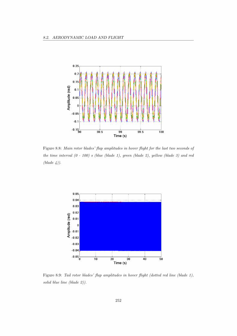
8.2. AERODYNAMIC LOAD AND FLIGHT
Figure 8.8: Main rotor blades’ flap amplitudes in hover flight for the last two seconds of
the time interval (0 - 100) s (blue (blade 1), green (blade 2), yellow (blade 3) and red
(blade 4)).
Figure 8.9: Tail rotor blades’ flap amplitudes in hover flight (dotted red line (blade 1),
solid blue line (blade 2)).
252

8.2. AERODYNAMIC LOAD AND FLIGHT
Figure 8.10: Zoom of figure 8.9. Tail rotor blades’ flap amplitudes in hover flight (dotted
red line (blade 1), solid blue line (blade 2)).
Figure 8.11: Induced velocity ratio as a function of climb velocity ratio based on mo-
mentun theory (complete induced velocity curve). Reproduced with permission from
Cambridge University Press [98].
253
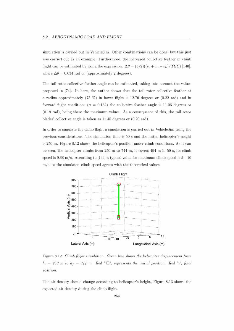
8.2. AERODYNAMIC LOAD AND FLIGHT
simulation is carried out in VehicleSim. Other combinations can be done, but this just
was carried out as an example. Furthermore, the increased collective feather in climb
flight can be estimated by using the expression: ∆θ = (3/2)((vc+vic−vh)/(ΩR)) [140],
where ∆θ = 0.034 rad or (approximately 2 degrees).
The tail rotor collective feather angle can be estimated, taking into account the values
proposed in [74]. In here, the author shows that the tail rotor collective feather at
a radius approximately (75 %) in hover flight is 12.70 degrees or (0.22 rad) and in
forward flight conditions (µ = 0.132) the collective feather angle is 11.06 degrees or
(0.19 rad), being these the maximum values. As a consequence of this, the tail rotor
blades’ collective angle is taken as 11.45 degrees or (0.20 rad).
In order to simulate the climb flight a simulation is carried out in VehicleSim using the
previous considerations. The simulation time is 50 s and the initial helicopter’s height
is 250 m. Figure 8.12 shows the helicopter’s position under climb conditions. As it can
be seen, the helicopter climbs from 250 m to 744 m, it covers 494 m in 50 s, its climb
speed is 9.88 m/s. According to [144] a typical value for maximum climb speed is 5−10
m/s, so the simulated climb speed agrees with the theoretical values.
Figure 8.12: Climb flight simulation. Green line shows the helicopter displacement from
hi = 250 m to hf = 744 m. Red ’ ’, represents the initial position. Red ’’, final
position.
The air density should change according to helicopter’s height, Figure 8.13 shows the
expected air density during the climb flight.
254
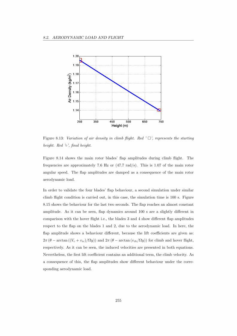
8.2. AERODYNAMIC LOAD AND FLIGHT
Figure 8.13: Variation of air density in climb flight. Red ’ ’, represents the starting
height. Red ’’, final height.
Figure 8.14 shows the main rotor blades’ flap amplitudes during climb flight. The
frequencies are approximately 7.6 Hz or (47.7 rad/s). This is 1.07 of the main rotor
angular speed. The flap amplitudes are damped as a consequence of the main rotor
aerodynamic load.
In order to validate the four blades’ flap behaviour, a second simulation under similar
climb flight condition is carried out, in this case, the simulation time is 100 s. Figure
8.15 shows the behaviour for the last two seconds. The flap reaches an almost constant
amplitude. As it can be seen, flap dynamics around 100 s are a slightly different in
comparison with the hover flight i.e., the blades 3 and 4 show different flap amplitudes
respect to the flap on the blades 1 and 2, due to the aerodynamic load. In here, the
flap amplitude shows a behaviour different, because the lift coefficients are given as:
2π (θ − arctan ((Vc + vic)/Ωy)) and 2π (θ − arctan (vih/Ωy)) for climb and hover flight,
respectively. As it can be seen, the induced velocities are presented in both equations.
Nevertheless, the first lift coefficient contains an additional term, the climb velocity. As
a consequence of this, the flap amplitudes show different behaviour under the corre-
sponding aerodynamic load.
255
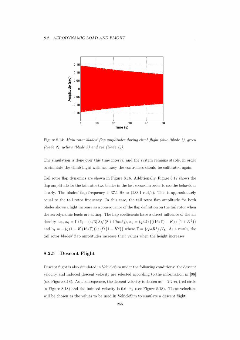
8.2. AERODYNAMIC LOAD AND FLIGHT
Figure 8.14: Main rotor blades’ flap amplitudes during climb flight (blue (blade 1), green
(blade 2), yellow (blade 3) and red (blade 4)).
The simulation is done over this time interval and the system remains stable, in order
to simulate the climb flight with accuracy the controllers should be calibrated again.
Tail rotor flap dynamics are shown in Figure 8.16. Additionally, Figure 8.17 shows the
flap amplitude for the tail rotor two blades in the last second in order to see the behaviour
clearly. The blades’ flap frequency is 37.1 Hz or (233.1 rad/s). This is approximately
equal to the tail rotor frequency. In this case, the tail rotor flap amplitude for both
blades shows a light increase as a consequence of the flap definition on the tail rotor when
the aerodynamic loads are acting. The flap coefficients have a direct influence of the air
density i.e., a0 = Γ (θ0 − (4/3)λ)/ (8 + Γtanδ3), a1 = (q/Ω)(((16/Γ)−K) /
(1 +K2
))and b1 = − (q (1 +K (16/Γ))) /
(Ω(1 +K2
))where Γ =
(cρaR4
)/If . As a result, the
tail rotor blades’ flap amplitudes increase their values when the height increases.
8.2.5 Descent Flight
Descent flight is also simulated in VehicleSim under the following conditions: the descent
velocity and induced descent velocity are selected according to the information in [98]
(see Figure 8.18). As a consequence, the descent velocity is chosen as: −2.2·vh (red circle
in Figure 8.18) and the induced velocity is 0.6 · vh (see Figure 8.18). These velocities
will be chosen as the values to be used in VehicleSim to simulate a descent flight.
256
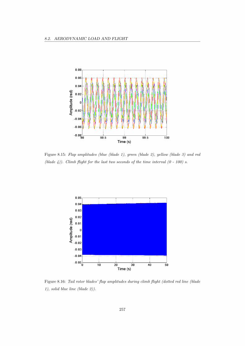
8.2. AERODYNAMIC LOAD AND FLIGHT
Figure 8.15: Flap amplitudes (blue (blade 1), green (blade 2), yellow (blade 3) and red
(blade 4)). Climb flight for the last two seconds of the time interval (0 - 100) s.
Figure 8.16: Tail rotor blades’ flap amplitudes during climb flight (dotted red line (blade
1), solid blue line (blade 2)).
257

8.2. AERODYNAMIC LOAD AND FLIGHT
Figure 8.17: Zoom of figure 8.16. Tail rotor blades’ flap amplitudes during climb flight
(dotted red line (blade 1), solid blue line (blade 2)).
Figure 8.18: Induced velocity variation as a function of descent velocity based on mo-
mentun theory (complete induced velocity curve). Reproduced with permission from
Cambridge University Press [98].
258
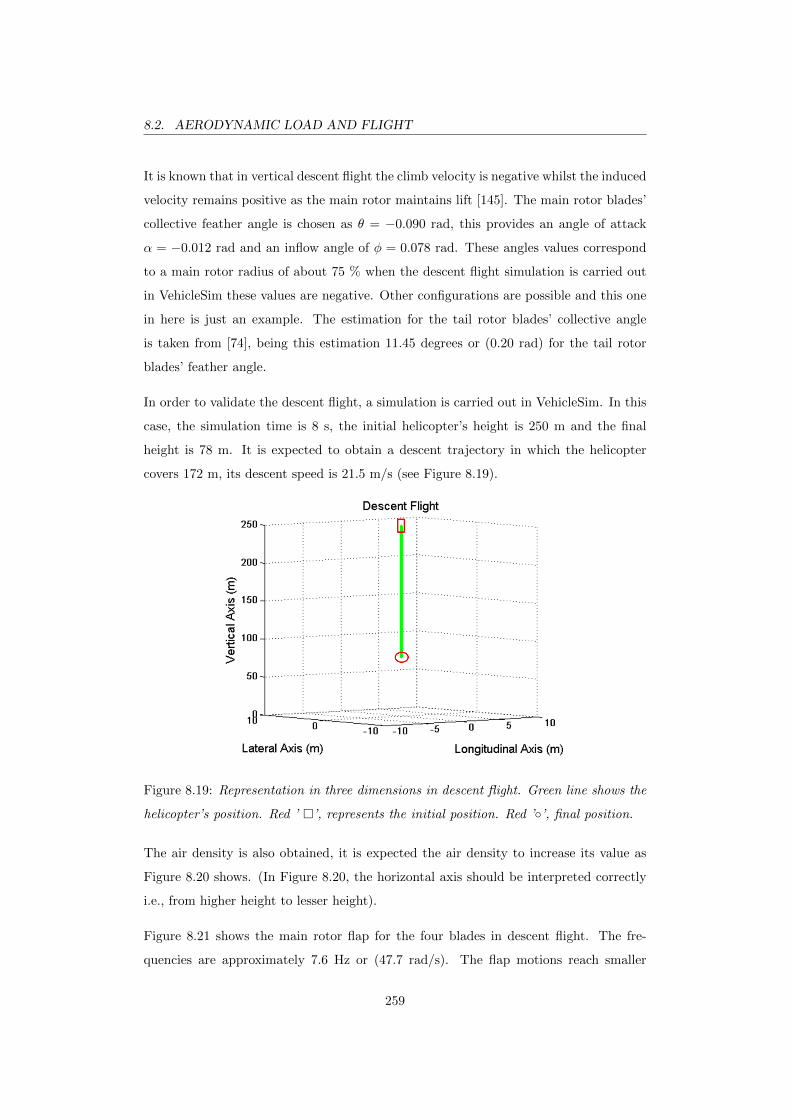
8.2. AERODYNAMIC LOAD AND FLIGHT
It is known that in vertical descent flight the climb velocity is negative whilst the induced
velocity remains positive as the main rotor maintains lift [145]. The main rotor blades’
collective feather angle is chosen as θ = −0.090 rad, this provides an angle of attack
α = −0.012 rad and an inflow angle of φ = 0.078 rad. These angles values correspond
to a main rotor radius of about 75 % when the descent flight simulation is carried out
in VehicleSim these values are negative. Other configurations are possible and this one
in here is just an example. The estimation for the tail rotor blades’ collective angle
is taken from [74], being this estimation 11.45 degrees or (0.20 rad) for the tail rotor
blades’ feather angle.
In order to validate the descent flight, a simulation is carried out in VehicleSim. In this
case, the simulation time is 8 s, the initial helicopter’s height is 250 m and the final
height is 78 m. It is expected to obtain a descent trajectory in which the helicopter
covers 172 m, its descent speed is 21.5 m/s (see Figure 8.19).
Figure 8.19: Representation in three dimensions in descent flight. Green line shows the
helicopter’s position. Red ’ ’, represents the initial position. Red ’’, final position.
The air density is also obtained, it is expected the air density to increase its value as
Figure 8.20 shows. (In Figure 8.20, the horizontal axis should be interpreted correctly
i.e., from higher height to lesser height).
Figure 8.21 shows the main rotor flap for the four blades in descent flight. The fre-
quencies are approximately 7.6 Hz or (47.7 rad/s). The flap motions reach smaller
259
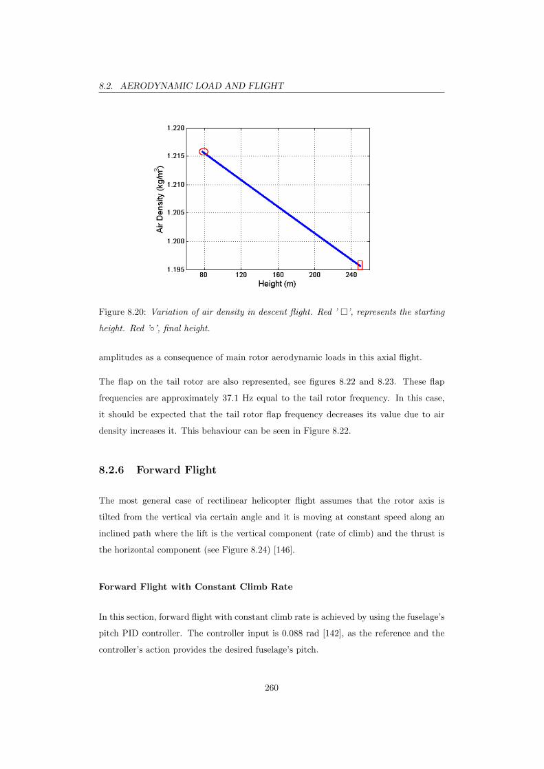
8.2. AERODYNAMIC LOAD AND FLIGHT
Figure 8.20: Variation of air density in descent flight. Red ’ ’, represents the starting
height. Red ’’, final height.
amplitudes as a consequence of main rotor aerodynamic loads in this axial flight.
The flap on the tail rotor are also represented, see figures 8.22 and 8.23. These flap
frequencies are approximately 37.1 Hz equal to the tail rotor frequency. In this case,
it should be expected that the tail rotor flap frequency decreases its value due to air
density increases it. This behaviour can be seen in Figure 8.22.
8.2.6 Forward Flight
The most general case of rectilinear helicopter flight assumes that the rotor axis is
tilted from the vertical via certain angle and it is moving at constant speed along an
inclined path where the lift is the vertical component (rate of climb) and the thrust is
the horizontal component (see Figure 8.24) [146].
Forward Flight with Constant Climb Rate
In this section, forward flight with constant climb rate is achieved by using the fuselage’s
pitch PID controller. The controller input is 0.088 rad [142], as the reference and the
controller’s action provides the desired fuselage’s pitch.
260
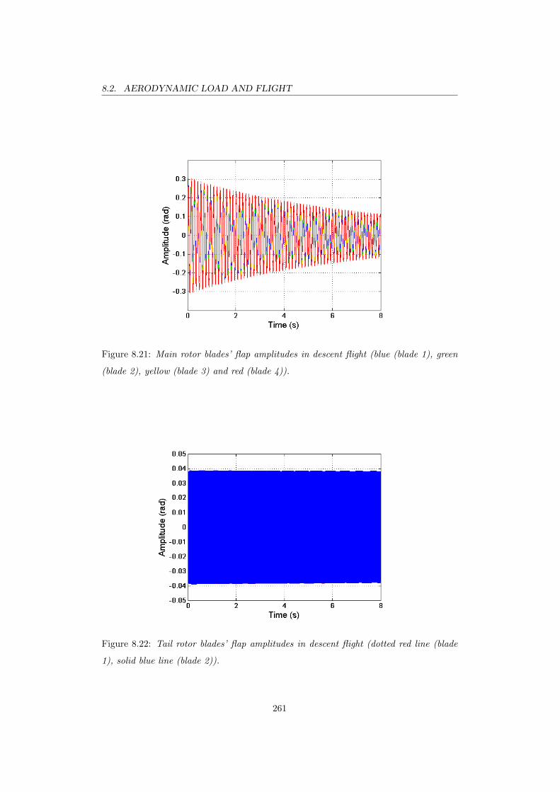
8.2. AERODYNAMIC LOAD AND FLIGHT
Figure 8.21: Main rotor blades’ flap amplitudes in descent flight (blue (blade 1), green
(blade 2), yellow (blade 3) and red (blade 4)).
Figure 8.22: Tail rotor blades’ flap amplitudes in descent flight (dotted red line (blade
1), solid blue line (blade 2)).
261
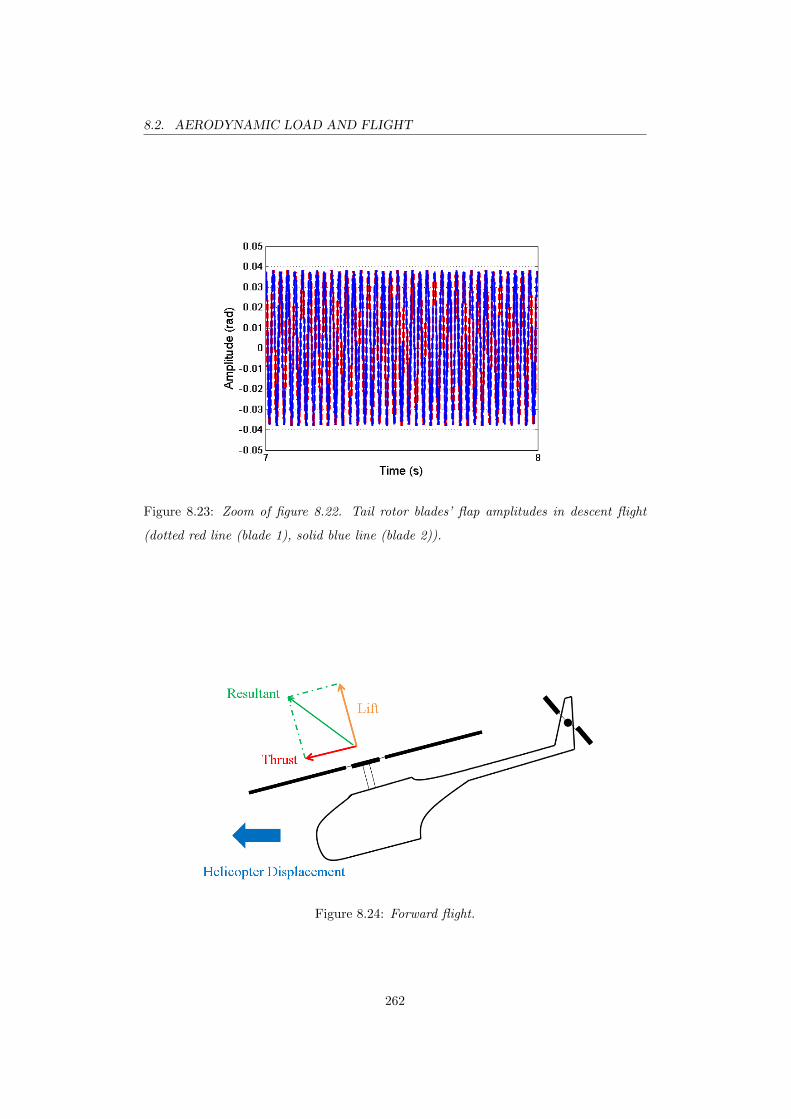
8.2. AERODYNAMIC LOAD AND FLIGHT
Figure 8.23: Zoom of figure 8.22. Tail rotor blades’ flap amplitudes in descent flight
(dotted red line (blade 1), solid blue line (blade 2)).
Figure 8.24: Forward flight.
262
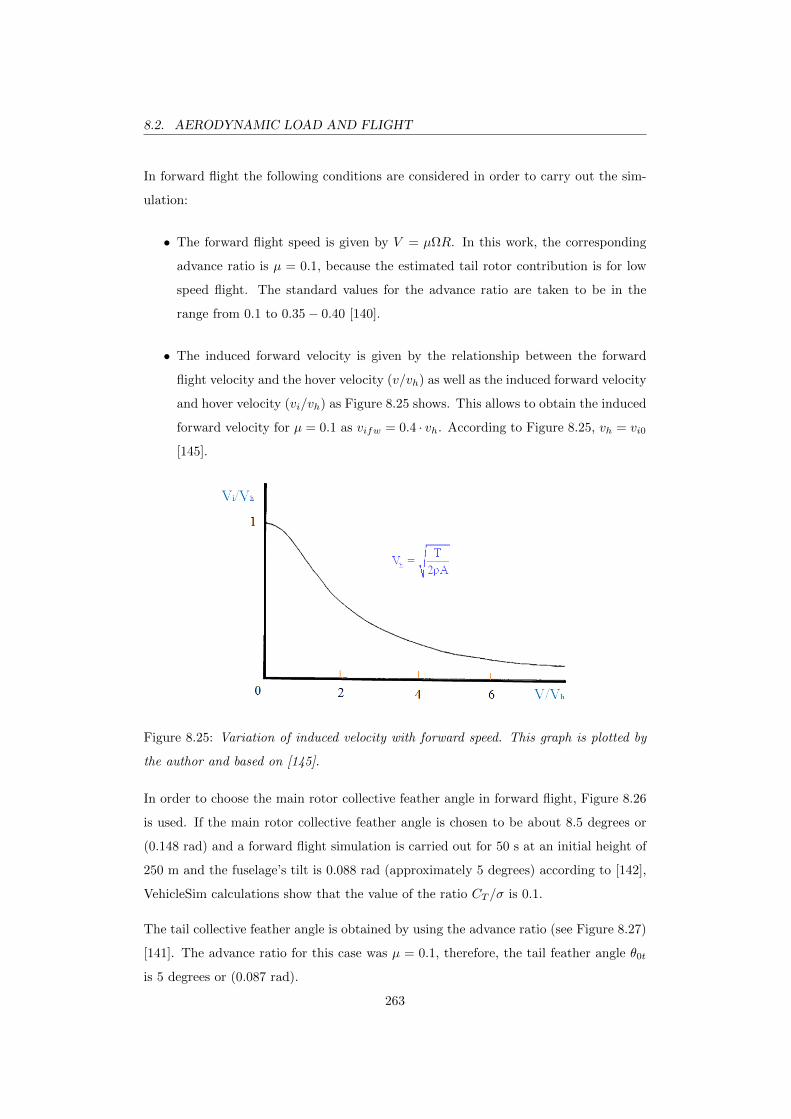
8.2. AERODYNAMIC LOAD AND FLIGHT
In forward flight the following conditions are considered in order to carry out the sim-
ulation:
• The forward flight speed is given by V = µΩR. In this work, the corresponding
advance ratio is µ = 0.1, because the estimated tail rotor contribution is for low
speed flight. The standard values for the advance ratio are taken to be in the
range from 0.1 to 0.35− 0.40 [140].
• The induced forward velocity is given by the relationship between the forward
flight velocity and the hover velocity (v/vh) as well as the induced forward velocity
and hover velocity (vi/vh) as Figure 8.25 shows. This allows to obtain the induced
forward velocity for µ = 0.1 as vifw = 0.4 · vh. According to Figure 8.25, vh = vi0
[145].
Figure 8.25: Variation of induced velocity with forward speed. This graph is plotted by
the author and based on [145].
In order to choose the main rotor collective feather angle in forward flight, Figure 8.26
is used. If the main rotor collective feather angle is chosen to be about 8.5 degrees or
(0.148 rad) and a forward flight simulation is carried out for 50 s at an initial height of
250 m and the fuselage’s tilt is 0.088 rad (approximately 5 degrees) according to [142],
VehicleSim calculations show that the value of the ratio CT /σ is 0.1.
The tail collective feather angle is obtained by using the advance ratio (see Figure 8.27)
[141]. The advance ratio for this case was µ = 0.1, therefore, the tail feather angle θ0t
is 5 degrees or (0.087 rad).
263
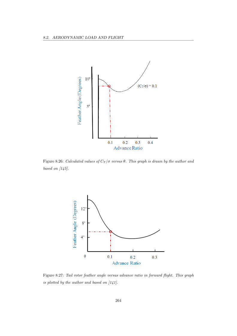
8.2. AERODYNAMIC LOAD AND FLIGHT
Figure 8.26: Calculated values of CT /σ versus θ. This graph is drawn by the author and
based on [145].
Figure 8.27: Tail rotor feather angle versus advance ratio in forward flight. This graph
is plotted by the author and based on [141].
264
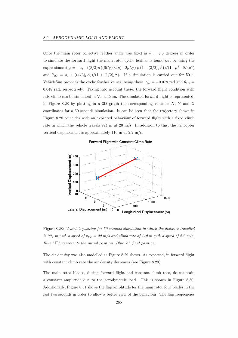
8.2. AERODYNAMIC LOAD AND FLIGHT
Once the main rotor collective feather angle was fixed as θ = 8.5 degrees in order
to simulate the forward flight the main rotor cyclic feather is found out by using the
expressions: θ1S = −a1−((8/3)µ ((6CT ) /σa)+2µλTPP(1− (3/2)µ2
))/(1−µ2+9/4µ4)
and θ1C = b1 + ((4/3)µa0)/(1 + (1/2)µ2). If a simulation is carried out for 50 s,
VehicleSim provides the cyclic feather values, being these θ1S = −0.078 rad and θ1C =
0.048 rad, respectively. Taking into account these, the forward flight condition with
rate climb can be simulated in VehicleSim. The simulated forward flight is represented,
in Figure 8.28 by plotting in a 3D graph the corresponding vehicle’s X, Y and Z
coordinates for a 50 seconds simulation. It can be seen that the trajectory shown in
Figure 8.28 coincides with an expected behaviour of forward flight with a fixed climb
rate in which the vehicle travels 994 m at 20 m/s. In addition to this, the helicopter
vertical displacement is approximately 110 m at 2.2 m/s.
Figure 8.28: Vehicle’s position for 50 seconds simulation in which the distance travelled
is 994 m with a speed of vfw = 20 m/s and climb rate of 110 m with a speed of 2.2 m/s.
Blue ’ ’, represents the initial position. Blue ’’, final position.
The air density was also modelled as Figure 8.29 shows. As expected, in forward flight
with constant climb rate the air density decreases (see Figure 8.29).
The main rotor blades, during forward flight and constant climb rate, do maintain
a constant amplitude due to the aerodynamic load. This is shown in Figure 8.30.
Additionally, Figure 8.31 shows the flap amplitude for the main rotor four blades in the
last two seconds in order to allow a better view of the behaviour. The flap frequencies
265
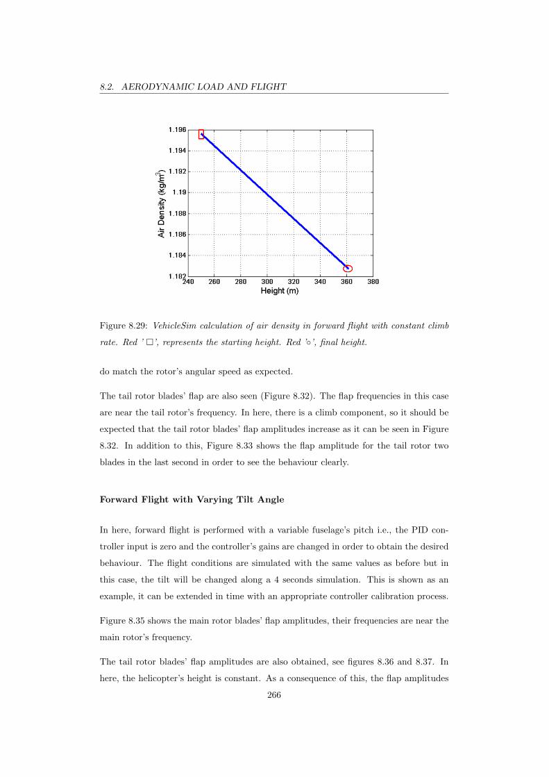
8.2. AERODYNAMIC LOAD AND FLIGHT
Figure 8.29: VehicleSim calculation of air density in forward flight with constant climb
rate. Red ’ ’, represents the starting height. Red ’’, final height.
do match the rotor’s angular speed as expected.
The tail rotor blades’ flap are also seen (Figure 8.32). The flap frequencies in this case
are near the tail rotor’s frequency. In here, there is a climb component, so it should be
expected that the tail rotor blades’ flap amplitudes increase as it can be seen in Figure
8.32. In addition to this, Figure 8.33 shows the flap amplitude for the tail rotor two
blades in the last second in order to see the behaviour clearly.
Forward Flight with Varying Tilt Angle
In here, forward flight is performed with a variable fuselage’s pitch i.e., the PID con-
troller input is zero and the controller’s gains are changed in order to obtain the desired
behaviour. The flight conditions are simulated with the same values as before but in
this case, the tilt will be changed along a 4 seconds simulation. This is shown as an
example, it can be extended in time with an appropriate controller calibration process.
Figure 8.35 shows the main rotor blades’ flap amplitudes, their frequencies are near the
main rotor’s frequency.
The tail rotor blades’ flap amplitudes are also obtained, see figures 8.36 and 8.37. In
here, the helicopter’s height is constant. As a consequence of this, the flap amplitudes
266
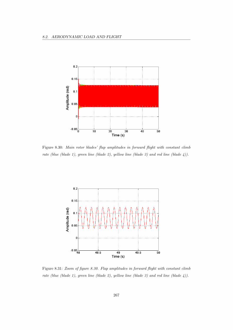
8.2. AERODYNAMIC LOAD AND FLIGHT
Figure 8.30: Main rotor blades’ flap amplitudes in forward flight with constant climb
rate (blue (blade 1), green line (blade 2), yellow line (blade 3) and red line (blade 4)).
Figure 8.31: Zoom of figure 8.30. Flap amplitudes in forward flight with constant climb
rate (blue (blade 1), green line (blade 2), yellow line (blade 3) and red line (blade 4)).
267
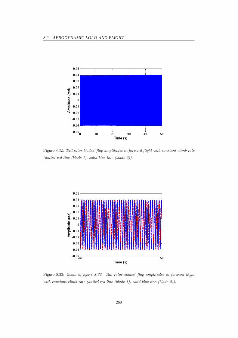
8.2. AERODYNAMIC LOAD AND FLIGHT
Figure 8.32: Tail rotor blades’ flap amplitudes in forward flight with constant climb rate
(dotted red line (blade 1), solid blue line (blade 2)).
Figure 8.33: Zoom of figure 8.32. Tail rotor blades’ flap amplitudes in forward flight
with constant climb rate (dotted red line (blade 1), solid blue line (blade 2)).
268
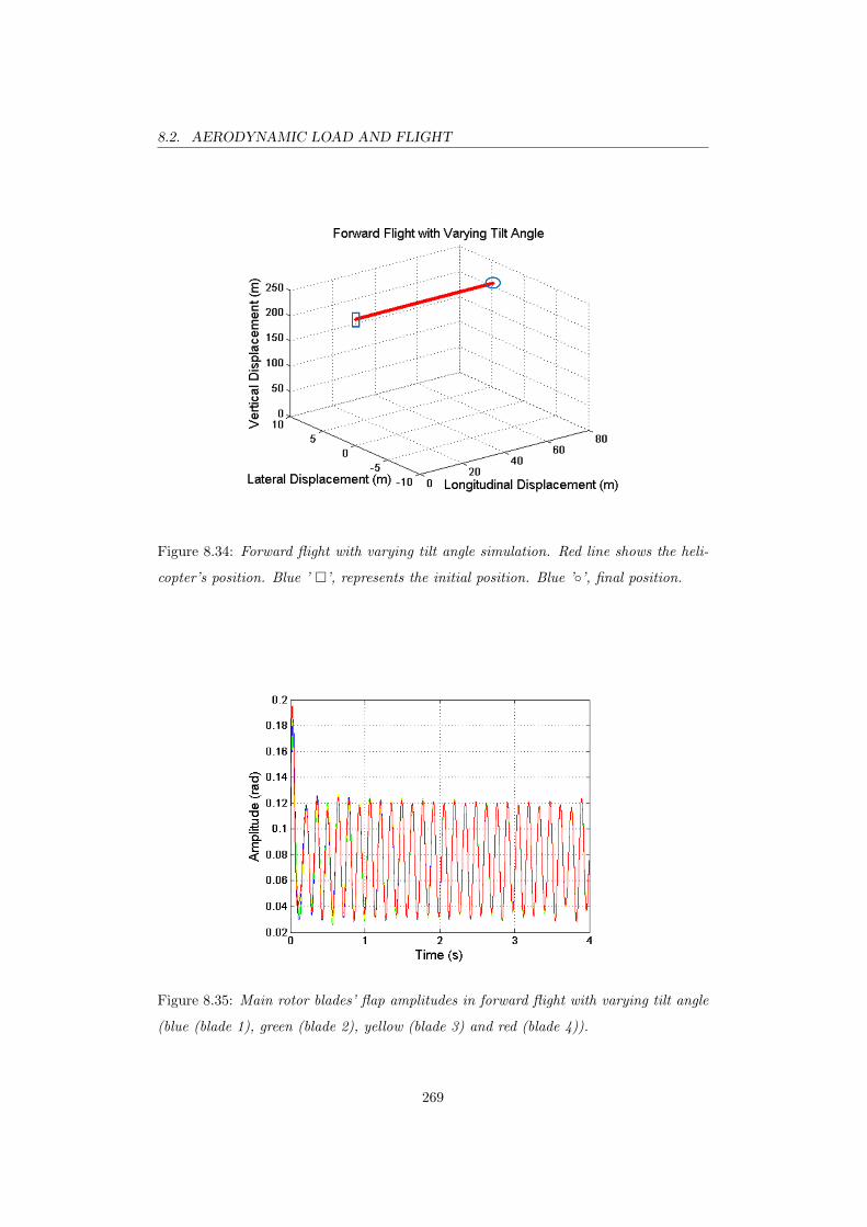
8.2. AERODYNAMIC LOAD AND FLIGHT
Figure 8.34: Forward flight with varying tilt angle simulation. Red line shows the heli-
copter’s position. Blue ’ ’, represents the initial position. Blue ’’, final position.
Figure 8.35: Main rotor blades’ flap amplitudes in forward flight with varying tilt angle
(blue (blade 1), green (blade 2), yellow (blade 3) and red (blade 4)).
269

8.2. AERODYNAMIC LOAD AND FLIGHT
remain constant according to the expected behaviour.
Figure 8.36: Tail rotor blades’ flap amplitudes in forward flight with varying tilt angle
(dotted red line (blade 1), solid blue line (blade 2)).
8.2.7 Trajectory Flight
Forward flight with constant climb rate can be also simulated for different orientations
in space i.e., the rates of yaw (ryaw) are changed using the fuselage’s yaw controller
defined in Chapter 6. Figure 8.38 shows three different trajectories under the action
of this controller for ryaw = 0.1 rad/s, ryaw = −0.1 rad/s and ryaw = −0.2 rad/s,
respectively.
Several combinations of various flight conditions are considered in order to simulate a
helicopter trajectory as Figure 8.39 shows. The trajectory starts with hover flight at a
height of h = 250 m for 4 s, then a climb flight from h = 250 m up to h = 279 m for
2 s is performed. After this, forward flight with a constant rate climb is performed for
30 s, its initial height is h = 279 m and its final height is 336 m. Then, hover flight is
simulated for 4 s at a constant height h = 336 m. Finally, a descent flight manoeuvre
from h = 336 m down to h = 254 m is simulated for 4 s.
This trajectory simulation was just an example on the achievable manoeuvring that can
be performed by the model here presented.
270

8.2. AERODYNAMIC LOAD AND FLIGHT
Figure 8.37: Zoom of figure 8.36. Tail rotor blades’ flap amplitudes in forward flight
with varying tilt angle (dotted red line (blade 1), solid blue line (blade 2)).
Figure 8.38: Several trajectories in forward flight with constant climb rate and different
rates of yaw (ryaw). Red line, represents ryaw = 0.1 rad/s. Green line, ryaw = -0.1
rad/s. Blue line, ryaw = -0.2 rad/s.
271
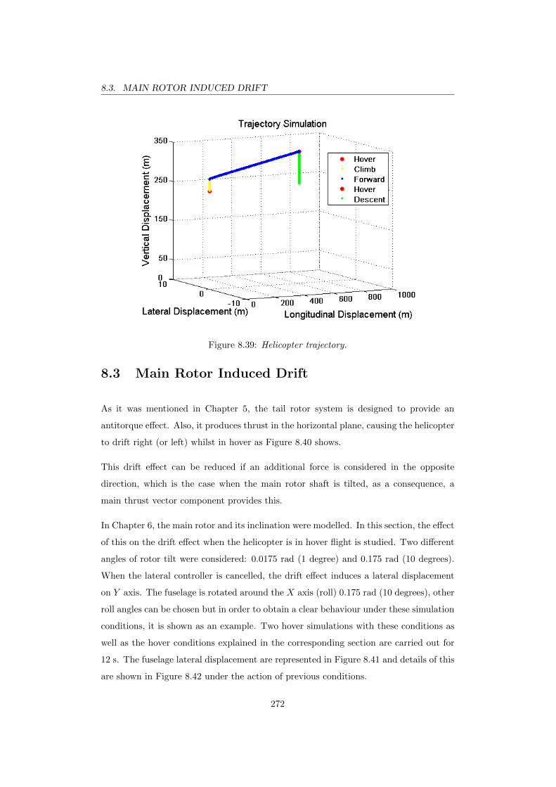
8.3. MAIN ROTOR INDUCED DRIFT
Figure 8.39: Helicopter trajectory.
8.3 Main Rotor Induced Drift
As it was mentioned in Chapter 5, the tail rotor system is designed to provide an
antitorque effect. Also, it produces thrust in the horizontal plane, causing the helicopter
to drift right (or left) whilst in hover as Figure 8.40 shows.
This drift effect can be reduced if an additional force is considered in the opposite
direction, which is the case when the main rotor shaft is tilted, as a consequence, a
main thrust vector component provides this.
In Chapter 6, the main rotor and its inclination were modelled. In this section, the effect
of this on the drift effect when the helicopter is in hover flight is studied. Two different
angles of rotor tilt were considered: 0.0175 rad (1 degree) and 0.175 rad (10 degrees).
When the lateral controller is cancelled, the drift effect induces a lateral displacement
on Y axis. The fuselage is rotated around the X axis (roll) 0.175 rad (10 degrees), other
roll angles can be chosen but in order to obtain a clear behaviour under these simulation
conditions, it is shown as an example. Two hover simulations with these conditions as
well as the hover conditions explained in the corresponding section are carried out for
12 s. The fuselage lateral displacement are represented in Figure 8.41 and details of this
are shown in Figure 8.42 under the action of previous conditions.
272
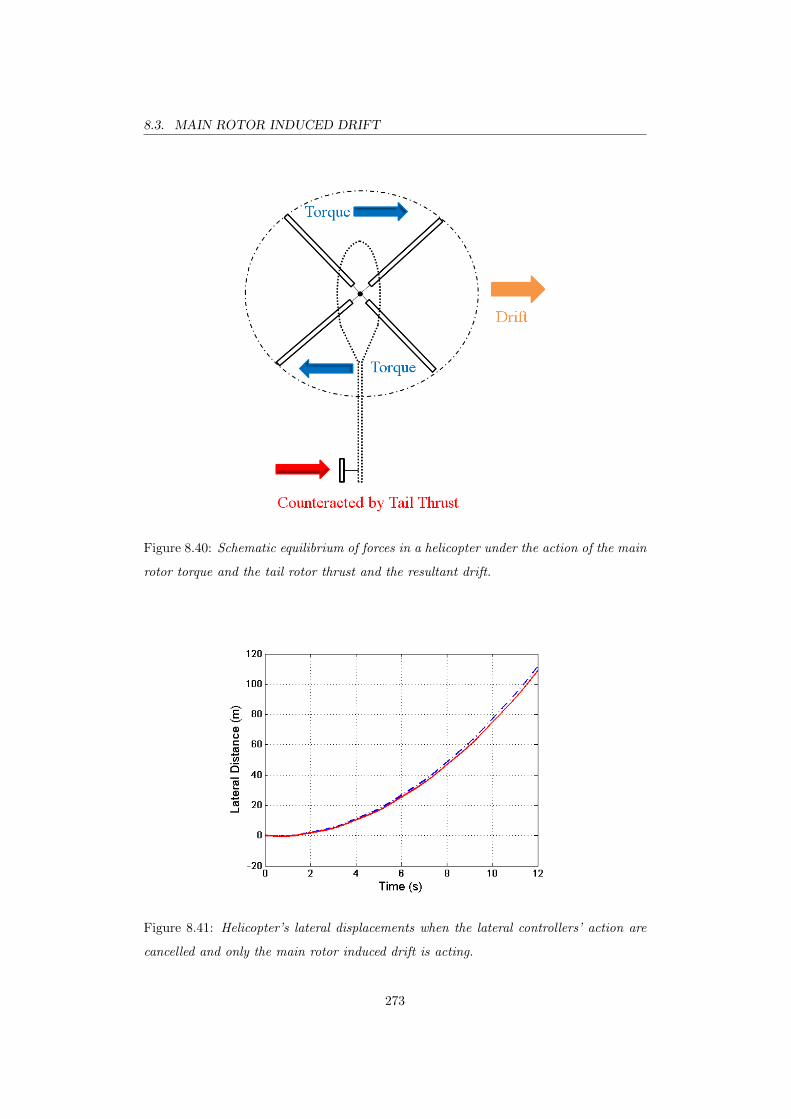
8.3. MAIN ROTOR INDUCED DRIFT
Figure 8.40: Schematic equilibrium of forces in a helicopter under the action of the main
rotor torque and the tail rotor thrust and the resultant drift.
Figure 8.41: Helicopter’s lateral displacements when the lateral controllers’ action are
cancelled and only the main rotor induced drift is acting.
273
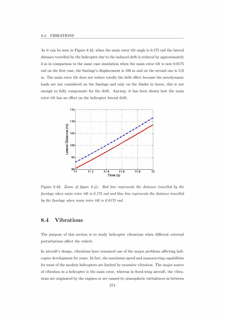
8.4. VIBRATIONS
As it can be seen in Figure 8.42, when the main rotor tilt angle is 0.175 rad the lateral
distance travelled by the helicopter due to the induced drift is reduced by approximately
3 m in comparison to the same case simulation when the main rotor tilt is now 0.0175
rad on the first case, the fuselage’s displacement is 108 m and on the second one is 112
m. The main rotor tilt does not reduce totally the drift effect because the aerodynamic
loads are not considered on the fuselage and only on the blades in hover, this is not
enough to fully compensate for the drift. Anyway, it has been shown how the main
rotor tilt has an effect on the helicopter lateral drift.
Figure 8.42: Zoom of figure 8.41. Red line represents the distance travelled by the
fuselage when main rotor tilt is 0.175 rad and blue line represents the distance travelled
by the fuselage when main rotor tilt is 0.0175 rad.
8.4 Vibrations
The purpose of this section is to study helicopter vibrations when different external
perturbations affect the vehicle.
In aircraft’s design, vibrations have remained one of the major problems affecting heli-
copter development for years. In fact, the maximum speed and manoeuvring capabilities
for most of the modern helicopters are limited by excessive vibration. The major source
of vibration in a helicopter is the main rotor, whereas in fixed-wing aircraft, the vibra-
tions are originated by the engines or are caused by atmospheric turbulences in between
274
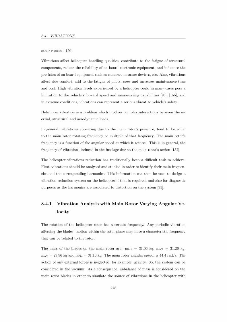
8.4. VIBRATIONS
other reasons [150].
Vibrations affect helicopter handling qualities, contribute to the fatigue of structural
components, reduce the reliability of on-board electronic equipment, and influence the
precision of on board equipment such as cameras, measure devices, etc. Also, vibrations
affect ride comfort, add to the fatigue of pilots, crew and increases maintenance time
and cost. High vibration levels experienced by a helicopter could in many cases pose a
limitation to the vehicle’s forward speed and manoeuvring capabilities [95], [155], and
in extreme conditions, vibrations can represent a serious threat to vehicle’s safety.
Helicopter vibration is a problem which involves complex interactions between the in-
ertial, structural and aerodynamic loads.
In general, vibrations appearing due to the main rotor’s presence, tend to be equal
to the main rotor rotating frequency or multiple of that frequency. The main rotor’s
frequency is a function of the angular speed at which it rotates. This is in general, the
frequency of vibrations induced in the fuselage due to the main rotor’s action [152].
The helicopter vibrations reduction has traditionally been a difficult task to achieve.
First, vibrations should be analysed and studied in order to identify their main frequen-
cies and the corresponding harmonics. This information can then be used to design a
vibration reduction system on the helicopter if that is required, and also for diagnostic
purposes as the harmonics are associated to distortion on the system [95].
8.4.1 Vibration Analysis with Main Rotor Varying Angular Ve-
locity
The rotation of the helicopter rotor has a certain frequency. Any periodic vibration
affecting the blades’ motion within the rotor plane may have a characteristic frequency
that can be related to the rotor.
The mass of the blades on the main rotor are: mbl1 = 31.06 kg, mbl2 = 31.26 kg,
mbl3 = 29.96 kg and mbl4 = 31.16 kg. The main rotor angular speed, is 44.4 rad/s. The
action of any external forces is neglected, for example: gravity. So, the system can be
considered in the vacuum. As a consequence, unbalance of mass is considered on the
main rotor blades in order to simulate the source of vibrations in the helicopter with
275

8.4. VIBRATIONS
the requiring amplitude to be detected in the spectrum under the action of a varying
rotating speed.
Varying Angular Velocity
When referring to the helicopter’s fuselage, the induced vibrations frequency may be
heterodyned by the rotor’s frequency and the frequencies experienced in the fuselage
may then be the frequencies of the sidebands.
It is known that when two signals of frequencies ±f1 and ±f2, are multiplied, the result
is that the frequencies of each must be added. This results in four frequencies, ±(f1+f2)
and ±(f1 − f2), one of them is the sum of the input frequencies and the other is the
difference between them. These are called sidebands. Sidebands are found extensively
in avionics, where the deliberate use of the process is called heterodyning [143].
In order to reproduce this behaviour in the helicopter model, the main rotor’s angular
speed is implemented in VehicleSim as varying by using a PD controller in order to
simulate the engine behaviour. The time dependant angular velocity is defined as [93]:
Ω(t) = Ω1 + Ω2cos(Ω3t) (8.5)
where Ω1, Ω2 and Ω3 are angular speeds in rad/s. Equation (8.5) can be written as:
Ω(t) = 2πf1 + 2πf2cos (2πf3t) (8.6)
where f1, f2 and f3 are the corresponding frequencies expressed in Hz.
The main rotor’s linear equation of motion obtained in VehicleSim is (see equation
(8.7)):
Ω[Irtz + Iblzcos2θ + Iblxsin
2θ +mbl
(y2bl + eR (eR+ 2ybl)
)− kd]
= kd
((2π)
2f1f2sin (2πf3t)
)− kp (2π (f1 + f2cos (2πf3t))− Ω)
− (2Iblx − 2Iblz) Ωθcosθsinθ
(8.7)
where kp and kd are the proportional and derivative controller gains. θ is the feather
angle. Irtz is the main rotor moment of inertial around the Z axis. Iblx and Iblz are
the blades moments of inertia around the X and Z axes, and ybl is the centre of mass
of the blade along the Y axis. Equation (8.7) is shown for a blade with flap, lag and
276
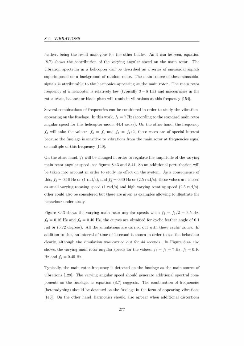
8.4. VIBRATIONS
feather, being the result analogous for the other blades. As it can be seen, equation
(8.7) shows the contribution of the varying angular speed on the main rotor. The
vibration spectrum in a helicopter can be described as a series of sinusoidal signals
superimposed on a background of random noise. The main source of these sinusoidal
signals is attributable to the harmonics appearing at the main rotor. The main rotor
frequency of a helicopter is relatively low (typically 3 − 8 Hz) and inaccuracies in the
rotor track, balance or blade pitch will result in vibrations at this frequency [154].
Several combinations of frequencies can be considered in order to study the vibrations
appearing on the fuselage. In this work, f1 = 7 Hz (according to the standard main rotor
angular speed for this helicopter model 44.4 rad/s). On the other hand, the frequency
f3 will take the values: f3 = f1 and f3 = f1/2, these cases are of special interest
because the fuselage is sensitive to vibrations from the main rotor at frequencies equal
or multiple of this frequency [140].
On the other hand, f2 will be changed in order to regulate the amplitude of the varying
main rotor angular speed, see figures 8.43 and 8.44. So an additional perturbation will
be taken into account in order to study its effect on the system. As a consequence of
this, f2 = 0.16 Hz or (1 rad/s), and f2 = 0.40 Hz or (2.5 rad/s), these values are chosen
as small varying rotating speed (1 rad/s) and high varying rotating speed (2.5 rad/s),
other could also be considered but these are given as examples allowing to illustrate the
behaviour under study.
Figure 8.43 shows the varying main rotor angular speeds when f3 = f1/2 = 3.5 Hz,
f2 = 0.16 Hz and f2 = 0.40 Hz, the curves are obtained for cyclic feather angle of 0.1
rad or (5.72 degrees). All the simulations are carried out with these cyclic values. In
addition to this, an interval of time of 1 second is shown in order to see the behaviour
clearly, although the simulation was carried out for 44 seconds. In Figure 8.44 also
shows, the varying main rotor angular speeds for the values: f3 = f1 = 7 Hz, f2 = 0.16
Hz and f2 = 0.40 Hz.
Typically, the main rotor frequency is detected on the fuselage as the main source of
vibrations [129]. The varying angular speed should generate additional spectral com-
ponents on the fuselage, as equation (8.7) suggests. The combination of frequencies
(heterodyning) should be detected on the fuselage in the form of appearing vibrations
[143]. On the other hand, harmonics should also appear when additional distortions
277
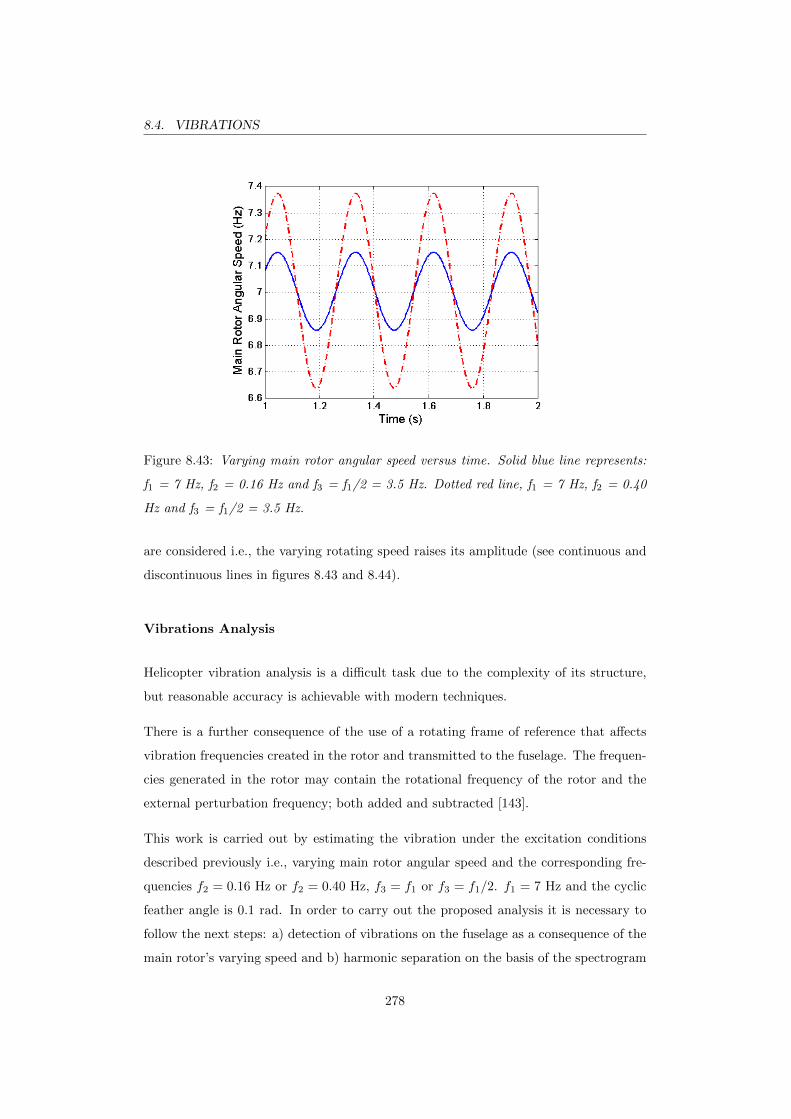
8.4. VIBRATIONS
Figure 8.43: Varying main rotor angular speed versus time. Solid blue line represents:
f1 = 7 Hz, f2 = 0.16 Hz and f3 = f1/2 = 3.5 Hz. Dotted red line, f1 = 7 Hz, f2 = 0.40
Hz and f3 = f1/2 = 3.5 Hz.
are considered i.e., the varying rotating speed raises its amplitude (see continuous and
discontinuous lines in figures 8.43 and 8.44).
Vibrations Analysis
Helicopter vibration analysis is a difficult task due to the complexity of its structure,
but reasonable accuracy is achievable with modern techniques.
There is a further consequence of the use of a rotating frame of reference that affects
vibration frequencies created in the rotor and transmitted to the fuselage. The frequen-
cies generated in the rotor may contain the rotational frequency of the rotor and the
external perturbation frequency; both added and subtracted [143].
This work is carried out by estimating the vibration under the excitation conditions
described previously i.e., varying main rotor angular speed and the corresponding fre-
quencies f2 = 0.16 Hz or f2 = 0.40 Hz, f3 = f1 or f3 = f1/2. f1 = 7 Hz and the cyclic
feather angle is 0.1 rad. In order to carry out the proposed analysis it is necessary to
follow the next steps: a) detection of vibrations on the fuselage as a consequence of the
main rotor’s varying speed and b) harmonic separation on the basis of the spectrogram
278
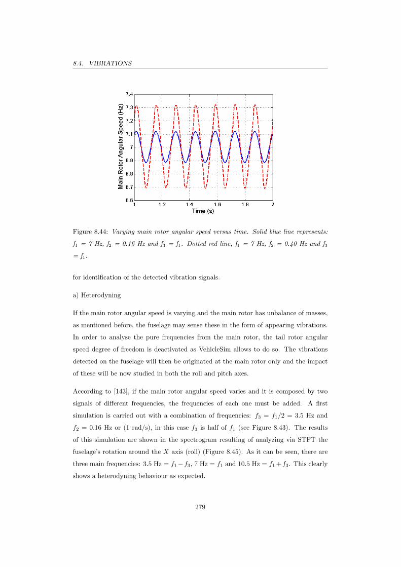
8.4. VIBRATIONS
Figure 8.44: Varying main rotor angular speed versus time. Solid blue line represents:
f1 = 7 Hz, f2 = 0.16 Hz and f3 = f1. Dotted red line, f1 = 7 Hz, f2 = 0.40 Hz and f3
= f1.
for identification of the detected vibration signals.
a) Heterodyning
If the main rotor angular speed is varying and the main rotor has unbalance of masses,
as mentioned before, the fuselage may sense these in the form of appearing vibrations.
In order to analyse the pure frequencies from the main rotor, the tail rotor angular
speed degree of freedom is deactivated as VehicleSim allows to do so. The vibrations
detected on the fuselage will then be originated at the main rotor only and the impact
of these will be now studied in both the roll and pitch axes.
According to [143], if the main rotor angular speed varies and it is composed by two
signals of different frequencies, the frequencies of each one must be added. A first
simulation is carried out with a combination of frequencies: f3 = f1/2 = 3.5 Hz and
f2 = 0.16 Hz or (1 rad/s), in this case f3 is half of f1 (see Figure 8.43). The results
of this simulation are shown in the spectrogram resulting of analyzing via STFT the
fuselage’s rotation around the X axis (roll) (Figure 8.45). As it can be seen, there are
three main frequencies: 3.5 Hz = f1−f3, 7 Hz = f1 and 10.5 Hz = f1 +f3. This clearly
shows a heterodyning behaviour as expected.
279
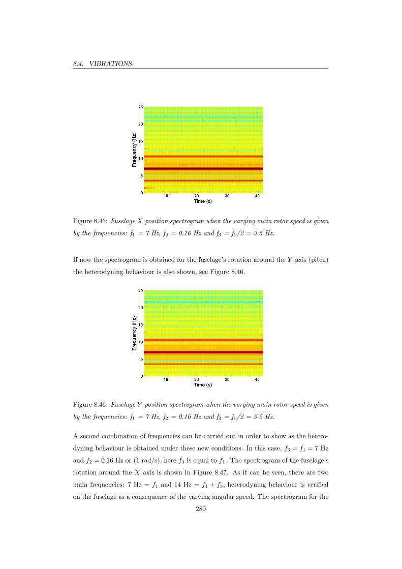
8.4. VIBRATIONS
Figure 8.45: Fuselage X position spectrogram when the varying main rotor speed is given
by the frequencies: f1 = 7 Hz, f2 = 0.16 Hz and f3 = f1/2 = 3.5 Hz.
If now the spectrogram is obtained for the fuselage’s rotation around the Y axis (pitch)
the heterodyning behaviour is also shown, see Figure 8.46.
Figure 8.46: Fuselage Y position spectrogram when the varying main rotor speed is given
by the frequencies: f1 = 7 Hz, f2 = 0.16 Hz and f3 = f1/2 = 3.5 Hz.
A second combination of frequencies can be carried out in order to show as the hetero-
dyning behaviour is obtained under these new conditions. In this case, f3 = f1 = 7 Hz
and f2 = 0.16 Hz or (1 rad/s), here f3 is equal to f1. The spectrogram of the fuselage’s
rotation around the X axis is shown in Figure 8.47. As it can be seen, there are two
main frequencies: 7 Hz = f1 and 14 Hz = f1 + f3, heterodyning behaviour is verified
on the fuselage as a consequence of the varying angular speed. The spectrogram for the
280

8.4. VIBRATIONS
fuselage rotation around the Y axis is represented in Figure 8.48: two main frequencies
are clearly identified, their values are 7 Hz and 14 Hz, this coincides with the expected
behaviour.
Figure 8.47: Fuselage X position spectrogram when the varying main rotor speed is given
by the frequencies: f1 = 7 Hz, f2 = 0.16 Hz and f3 = f1 = 7 Hz.
Figure 8.48: Fuselage Y position spectrogram when the varying main rotor speed is given
by the frequencies: f1 = 7 Hz, f2 = 0.16 Hz and f3 = f1 = 7 Hz.
The rotor angular speed with these simulations, it has been shown that results in vi-
brations that affect the fuselage roll and pitch, and their sidebands are as expected.
b) Heterodyning and Increase in Varying Rotation Speed
The identification of existing sidebands is a strong indicator of failures in mechanical
systems. The presence of harmonic or modulation series is then used as indicators of
distortion or damage of one or more parts of a mechanical system. Mathematically,
281
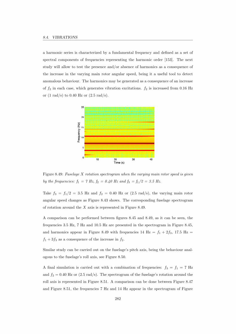
8.4. VIBRATIONS
a harmonic series is characterized by a fundamental frequency and defined as a set of
spectral components of frequencies representing the harmonic order [153]. The next
study will allow to test the presence and/or absence of harmonics as a consequence of
the increase in the varying main rotor angular speed, being it a useful tool to detect
anomalous behaviour. The harmonics may be generated as a consequence of an increase
of f2 in each case, which generates vibration excitations. f2 is increased from 0.16 Hz
or (1 rad/s) to 0.40 Hz or (2.5 rad/s).
Figure 8.49: Fuselage X rotation spectrogram when the varying main rotor speed is given
by the frequencies: f1 = 7 Hz, f2 = 0.40 Hz and f3 = f1/2 = 3.5 Hz.
Take f3 = f1/2 = 3.5 Hz and f2 = 0.40 Hz or (2.5 rad/s), the varying main rotor
angular speed changes as Figure 8.43 shows. The corresponding fuselage spectrogram
of rotation around the X axis is represented in Figure 8.49.
A comparison can be performed between figures 8.45 and 8.49, as it can be seen, the
frequencies 3.5 Hz, 7 Hz and 10.5 Hz are presented in the spectrogram in Figure 8.45,
and harmonics appear in Figure 8.49 with frequencies 14 Hz = f1 + 2f3, 17.5 Hz =
f1 + 3f3 as a consequence of the increase in f2.
Similar study can be carried out on the fuselage’s pitch axis, being the behaviour anal-
ogous to the fuselage’s roll axis, see Figure 8.50.
A final simulation is carried out with a combination of frequencies: f3 = f1 = 7 Hz
and f2 = 0.40 Hz or (2.5 rad/s). The spectrogram of the fuselage’s rotation around the
roll axis is represented in Figure 8.51. A comparison can be done between Figure 8.47
and Figure 8.51, the frequencies 7 Hz and 14 Hz appear in the spectrogram of Figure
282

8.4. VIBRATIONS
Figure 8.50: Fuselage Y rotation spectrogram when the varying main rotor speed is given
by the frequencies: f1 = 7 Hz, f2 = 0.40 Hz and f3 = f1/2 = 3.5 Hz.
8.47, and harmonics appear with frequencies 21 Hz = f1 + 2f3, 28 Hz = f1 + 3f3, 42 Hz
= f1 + 5f3 appear in the results shown in Figure 8.51.
Similarly, a spectrogram is obtained for the fuselage pitch axis rotation. As it can
be seen in Figure 8.52, the spectrogram shows similar sequences of harmonics as the
fuselage was showing in the case of X axis for this combination of frequencies.
Figure 8.51: Fuselage X rotation spectrogram when the varying main rotor speed is given
by the frequencies: f1 = 7 Hz, f2 = 0.40 Hz and f3 = f1 = 7 Hz.
The reason of this analysis is to study the effects on the fuselage’s rotation (X and Y
axes) spectrograms that the increase of f2 has. The changes introduced in the rotor
angular speed have an impact in the fuselage in the form of vibrations and subsequent
harmonics that appear as expected from theoretical predictions.
283
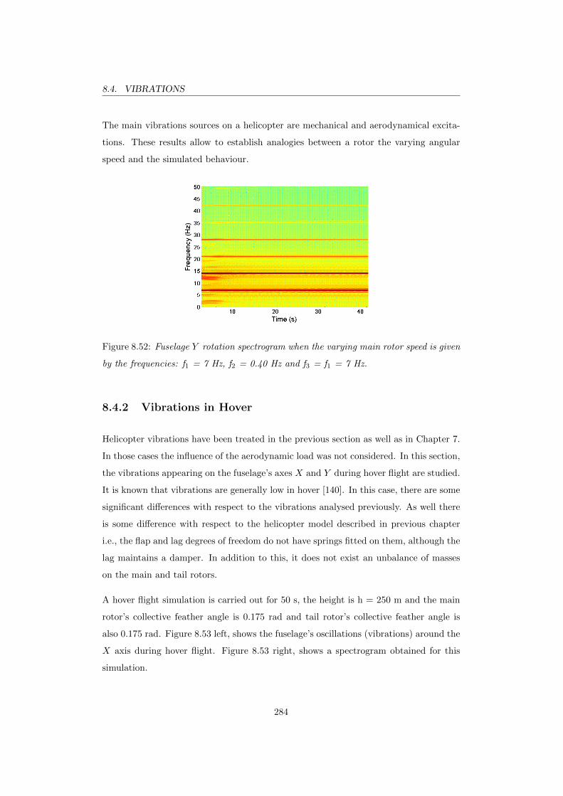
8.4. VIBRATIONS
The main vibrations sources on a helicopter are mechanical and aerodynamical excita-
tions. These results allow to establish analogies between a rotor the varying angular
speed and the simulated behaviour.
Figure 8.52: Fuselage Y rotation spectrogram when the varying main rotor speed is given
by the frequencies: f1 = 7 Hz, f2 = 0.40 Hz and f3 = f1 = 7 Hz.
8.4.2 Vibrations in Hover
Helicopter vibrations have been treated in the previous section as well as in Chapter 7.
In those cases the influence of the aerodynamic load was not considered. In this section,
the vibrations appearing on the fuselage’s axes X and Y during hover flight are studied.
It is known that vibrations are generally low in hover [140]. In this case, there are some
significant differences with respect to the vibrations analysed previously. As well there
is some difference with respect to the helicopter model described in previous chapter
i.e., the flap and lag degrees of freedom do not have springs fitted on them, although the
lag maintains a damper. In addition to this, it does not exist an unbalance of masses
on the main and tail rotors.
A hover flight simulation is carried out for 50 s, the height is h = 250 m and the main
rotor’s collective feather angle is 0.175 rad and tail rotor’s collective feather angle is
also 0.175 rad. Figure 8.53 left, shows the fuselage’s oscillations (vibrations) around the
X axis during hover flight. Figure 8.53 right, shows a spectrogram obtained for this
simulation.
284
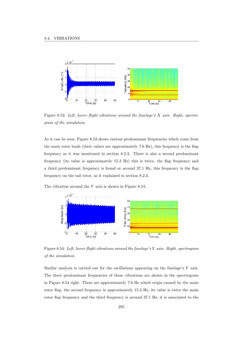
8.4. VIBRATIONS
Figure 8.53: Left, hover flight vibrations around the fuselage’s X axis. Right, spectro-
gram of the simulation.
As it can be seen, Figure 8.53 shows various predominant frequencies which come from
the main rotor loads (their values are approximately 7.6 Hz), this frequency is the flap
frequency as it was mentioned in section 8.2.3. There is also a second predominant
frequency (its value is approximately 15.2 Hz) this is twice, the flap frequency and
a third predominant frequency is found at around 37.1 Hz, this frequency is the flap
frequency on the tail rotor, as it explained in section 8.2.3.
The vibration around the Y axis is shown in Figure 8.54.
Figure 8.54: Left, hover flight vibrations around the fuselage’s Y axis. Right, spectrogram
of the simulation.
Similar analysis is carried out for the oscillations appearing on the fuselage’s Y axis.
The three predominant frequencies of these vibrations are shown in the spectrogram
in Figure 8.54 right. These are approximately 7.6 Hz which origin caused by the main
rotor flap, the second frequency is approximately 15.2 Hz, its value is twice the main
rotor flap frequency and the third frequency is around 37.1 Hz, it is associated to the
285

8.5. CHAPTER SUMMARY
tail rotor flap motion.
As it can be seen, the aerodynamic loads are sources of vibrations on the helicopter’s
fuselage. The spectrograms in hover flight obtained under the influence of aerodynamic
loads agree with the theoretical prediction: a) there is an important source of helicopter
vibration, the aerodynamics forces [140], b) the aerodynamic loads on a helicopter rotor
blade vary considerably as it moves around the rotor disc. These loads arise from the
aerodynamic forces on the rotor blades, together with the inertial forces produced by
the flap and lag motions of the blade [141].
8.5 Chapter Summary
The aim of this chapter was to show that external forces such as gravity, aerodynamic
loads and varying angular speed on the main rotor can be simulated in VehicleSim and
their effects can be analysed and studied.
The first external force to be added into the model is the gravity, its influence on the
rotorcraft has been shown and the ground action has been modelled on the fuselage.
The equilibrium positions for the blades on the main and tail rotors have been also
simulated under the action of gravity.
The nonlinear aerodynamic equations for flap and lag motion as well as lift and drag
forces were modelled and full details of their validation have been provided.
On the other hand, hover, climb, descent and forward flight conditions have been sim-
ulated and the parameters used in each case have been carefully described as well as
the flight conditions. Several trajectories in forward flight have been simulated in order
to show that the modelled helicopter can fly with different orientation in the space.
Besides, combinations of different flight conditions have been done. In this way, it has
been shown as the helicopter model here presented is capable of performing trajectories.
In addition to this, a model in which the main rotor angular speed is not constant and
changes by means of a PD controller has been presented. This allows to obtain different
combinations of frequencies between the main rotor standard frequency and external
varying frequencies, this combination of frequencies is important in order to study and
analyze the vibrations appearing in the fuselage as a consequence of these perturbations.
286
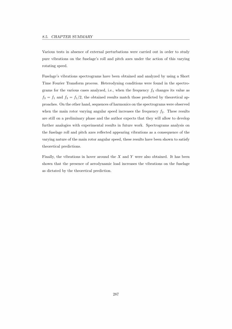
8.5. CHAPTER SUMMARY
Various tests in absence of external perturbations were carried out in order to study
pure vibrations on the fuselage’s roll and pitch axes under the action of this varying
rotating speed.
Fuselage’s vibrations spectrograms have been obtained and analyzed by using a Short
Time Fourier Transform process. Heterodyning conditions were found in the spectro-
grams for the various cases analyzed, i.e., when the frequency f3 changes its value as
f3 = f1 and f3 = f1/2, the obtained results match those predicted by theoretical ap-
proaches. On the other hand, sequences of harmonics on the spectrograms were observed
when the main rotor varying angular speed increases the frequency f2. These results
are still on a preliminary phase and the author expects that they will allow to develop
further analogies with experimental results in future work. Spectrograms analysis on
the fuselage roll and pitch axes reflected appearing vibrations as a consequence of the
varying nature of the main rotor angular speed, these results have been shown to satisfy
theoretical predictions.
Finally, the vibrations in hover around the X and Y were also obtained. It has been
shown that the presence of aerodynamic load increases the vibrations on the fuselage
as dictated by the theoretical prediction.
287

Part IV
Conclusions
288

Chapter 9
Conclusions and Future Work
9.1 Conclusions
9.1.1 Main Findings
The motivation of this work came from the need to provide a comprehensive helicopter
model, that is not too computationally demanding to implement and could be used for
control applications, stability analysis, etc. In particular, a detailed helicopter simu-
lation model using VehicleSim has been developed. It has been shown that the very
preliminary results obtained in Autosim by Tomas-Rodriguez [124], [125], can be ex-
panded by the multibody modelling code VehicleSim in order to build up a high fidelity
helicopter model on Sikorsky configuration that accounts for both dynamics and aero-
dynamics. The approach developed in here provides a robust model of a helicopter,
VehicleSim gives this in the sense of modelling uncertainties because it is usual on the
modelling process to perform linearisations that fail to capture some of fundamental
nonlinear dynamics and couplings. In addition to this, automated equations obtained
using this software provide an accurate representation of the complex system’s dynam-
ics. VehicleSim commands have been used to describe the components of the helicopter
multibody system in a parent-child relationship according to their physical constraints
and joints. Furthermore, VehicleSim code has been used to generate a C simulation pro-
gram, capable of computing general motions corresponding to specific initial conditions
289
9.1. CONCLUSIONS
and external forcing inputs.
9.1.2 Contribution to the Knowledge
Both linear and nonlinear equations for the main rotor flap and lag degrees of freedom
and flap-lag coupling as well as feather (all this in vacuum conditions) have been pro-
vided and all of them have been validated with the existing theory. Two appendices
are included in order to validate with analytical mechanical equations the flap and lag
expressions obtained from VehicleSim. The effects of various values of blade offset and
springs stiffness fitted on the blades’ hinges were analyzed for the flap and lag cases, and
the obtained results proved to be correct by theory validation. Main rotor flap and lag
degrees of freedom have been validated using a frequency domain approach in absence
of external forces. Fuselage and main rotor interaction has been studied and validated
using modal analysis. In fact, the stability of the system has been studied using the
root locus methodology. This was carried out as the full nonlinear equations of motion
of the helicopter model were obtained in C, time histories generated and the linearised
state-space model was also obtained in symbolic form as a Matlab m-file. A typical lo-
cal stability study in VehicleSim requires the importation of quasi-steady time histories
from the nonlinear simulation to the symbolic linearised equations of motion. In addi-
tion to this, the shape modes have been analyzed using modal analysis, and the results
showed the existence of a coupling between the fuselage vertical displacement and the
main rotor blade flap mode. The influence of the mass ratio, massblade/massfuselage,
on the coupled modes was demonstrated, and the influence of the lag degree of freedom
on the fuselage was also analyzed. The fuselage influence on the flap was studied as
a consequence of the gyroscopic movement on the fuselage. The results showed good
agreement with the theoretical findings existing in the literature.
Dynamic vibrations (mainly from the main rotor) appearing on the fuselage have been as
well studied, being an unbalance of mass the main source of vibrations. Vibrations orig-
inated at the main rotor were simulated and their effects on the fuselage were studied;
first, the offset of the flap hinge and its effect on the fuselage were considered. Secondly,
the lag hinge vibrations due to the applied dynamic load. Furthermore, an unbalance
of mass on both rotors was taken into account and analyzed, being the frequencies
of the obtained vibrations in agreement to the expected results. Fuselage vibration
290
9.1. CONCLUSIONS
spectrograms were obtained and analyzed by using a Short Time Fourier Transform
process.
The tail rotor was modelled as well as the flap and feather degrees of freedom on this
rotor. The coupling flap-feather (via delta three angle) has been modelled and validated
with theoretical results. In fact, for various cases, it was shown how the flap frequencies
increased as a function of the advance ratio as a consequence of this coupling.
Both main and tail rotors angular speeds have been implemented by using PID con-
trollers. This allows to simulate the torques on both rotors. Furthermore, the heli-
copter’s six degrees of freedom were controlled around the equilibrium position i.e., the
point (0, 0, 0). The action of the external forces on the system adds extra complexity
in the modelling process. Gravity was the first external force added to the system in
absence of aerodynamic forces. The ground was simulated on the fuselage, this showed
that the fuselage remains around the equilibrium point (0, 0, 0) when this is adequately
modelled.
A helicopter aerodynamic model has also been built using blade element theory on the
main and tail rotors. Nonlinear aerodynamic have been modelled and they have been
validated with specialist literature. Hover, climb, descent and forward flight have been
simulated. The orientation in space has been shown as well as the corresponding forward
trajectories when the aerodynamic model is acting. Different flight conditions can be
combined and simulated to allow the model to follow certain trajectories.
Rotor tilt was considered and modelled on the main rotor as real helicopters do. The
effect that tilt has on the system was studied on hover flight conditions. The results
showed that the tilt on the main rotor has a contribution on the drift effect: under the
simulation conditions taken into account in this work, the tilt on the main rotor slightly
reduces the drift effect.
Vibrations when an external perturbation is acting on the main rotor such as varying an-
gular speed have been studied according to the expression Ω(t) = 2πf1+2πf2cos (2πf3t)
where f1 is the main rotor frequency and f2 and f3 are the corresponding external fre-
quencies expressed in Hz. In fact, a model in which the main rotor angular speed is
not constant and changes by means of a PD controller has been induced in the model.
This allows to obtain different combinations of frequencies between the main rotor stan-
dard frequency and the external varying frequencies, the combination of frequencies are
291
9.1. CONCLUSIONS
important in order to study and analyze the vibrations appearing in the fuselage as a
consequence of these perturbations. Various tests in absence of external perturbations
were carried out in order to study pure vibrations on the fuselage’s roll and pitch axes
under the action of only the main rotor varying angular speed.
Heterodyning conditions were found in the spectrograms for the various cases considered
i.e., when frequency f3 changes its value as f3 = f1 and f3 = f1/2, the obtained results
match those predicted by theoretical approaches. On the other hand, sequences of
harmonics on the spectrograms were observed when the main rotor varying angular
speed increases the frequency f2. Finally, aerodynamic vibrations in hover flight have
been simulated and analyzed, showing that the aerodynamic forces have the expected
behaviour if the vibrations are compared to the vibrations obtained in absence of the
external forces i.e., the noise is increased and the spectral components are larger.
On the other hand, an UAV helicopter dynamical model has also been modelled. This
model has been developed under the umbrella of an academic collaboration with ULL
(La Laguna University, Spain). Previous theoretical knowledge was used to model as
well as to implement this helicopter model. Moreover, this model was used to analyze
the vibrations appearing on the fuselage as a consequence of mass imbalance on the
main rotor, the vibrations obtained were analysed using a FFT (Fast Fourier Transform)
Matlab algorithm and these results agreed with experimental values proposed by various
authors. Once the model was built in VehicleSim and validated, La Laguna University
developed a robust control methodology for an onboard vision system.
During the timeframe in which this work has been carried out, journal articles have
been published as well as conference contributions have been made:
1) Marichal, G. N., Tomas-Rodriguez, M., Hernandez, A., Castillo-Rivera, S., Campoy,
P. Vibration Reduction for Vision Systems on Board UAV Using a Neuro-Fuzzy Con-
troller. June 2013. Journal of Control and Vibrations. 25, pp. 1-12. SAGE Journals,
2013. ISSN 1077-5463.
2) Marichal-Plasencia, G. N., Tomas-Rodriguez, M., Castillo-Rivera, S., Hernandez-
Lopez, A. Modelling and Analysis of Vibrations in a UAV Helicopter with a Vision
System. 2012. International Journal of Advanced Robotic Systems. Vol. 9, 220.
ISSN:1729-8806.
292
9.1. CONCLUSIONS
3) Castillo-Rivera, S., Tomas-Rodriguez, M., Marichal-Plasencia, G. N. Helicopter Main
Rotor Vibration Analysis with Varying Rotating Speed. XXXV Conference of Automa-
tion. Valencia 3-5 September 2014. Spain. pp. 34-41. ISBN-13: 978-84-697-5089-6.
4) Castillo-Rivera, S., Tomas-Rodriguez, M., Marichal-Plasencia, G. N., Hernandez-
Lopez, A. Estudio de la Interaccion del Fuselaje y el Movimiento de Aleteo de las Palas
del Rotor Principal en un Helicoptero. XXXIV Conference of Automation. Terrassa 4-6
September 2013. Spain. pp. 514-521. ISBN 978-84-616-5063-7.
5) Marichal-Plasencia, G. N., Tomas-Rodriguez, M., Campoy, P., Hernandez-Lopez, A.,
Castillo-Rivera, S. Reduccion de las Vibraciones de un Sistema de Vision a Bordo de un
Helicoptero Mediante un Controlador Inteligente. XXXIII Conference of Automation.
Vigo 5-7 September 2012. Spain. pp. 179-186. ISBN 978-84-8158-5834.
6) Marichal-Plasencia, G. N., Tomas-Rodriguez, M., Campoy, P., Castillo-Rivera, S.,
Hernandez-Lopez, A. Generacion de Vibraciones a Partir de la Simulacion de un Heli-
coptero para el Estudio de Sus Efectos Sobre el Sistema de Vision. XXXII Conference
of Automation. Sevilla 7-9 September 2011. Spain. ISBN 978-84-694-6454-0.
9.1.3 Scope of the Investigation
The presented work has several limitations as the blades are rigid in both rotors.
The fuselage’s aerodynamic effects have not been taken into account. The aerodynamic
modelling was focused only on both rotors using blade element theory.
The ground effect is not simulated as neither it is the landing and take off manoeuvre on
the ground. In addition to this, hover, climb, descent and forward flight are simulated
with an initial height of h = 250 m as well as different trajectories. On the contrary, other
heights could be selected when the controllers’ gains are calibrated for the corresponding
reference.
In conclusion, a full dynamical helicopter model was presented as well as an aerodynamic
model. The complexity involved in the modelling process helicopter has been explained
and evidenced. The need for automated methods in the analysis of such systems has
been demonstrated. This work opens the door for future helicopter studies as this
model provides the basis for not too complicated approach to these type of vehicles,
293
9.2. FUTURE WORK
with the guarantee of being a validated model, in which nonlinearities and couplings
(often simplified in the current existing models) are captured and maintained, increasing
in this way the fidelity of the future research carried out on this work.
9.2 Future Work
Several tasks could be completed as future work and in fact, some of them are being
explored at present.
9.2.1 Helicopter Model Improvements
In this work, the blades were assumed to be rigid bodies and they have been modelled as
such. In the improved helicopter model, an implementation of flexible blades would be
possible using VehicleSim. In order to carry this out, the blades could be divided into,
for example, twenty blade elements. Each blade element would have a degree of freedom
respect to the previous one. In addition to this, the flexibility between each of them
could be modelled with a spring on each blade element. Their values would be selected
using optimization methods that the author is currently studying. The optimization
could be carried out by comparison with blade flexibility parameters according to the
helicopter model used in this work.
One interesting result would be to characterize the fuselage’s flexibility. A finite-element
fuselage’s model can be used to obtain mode shapes of the flexible structure. This will
allow to study the coupled main rotor and fuselage. As a consequence of this, new mode
shapes will appear and the corresponding studies could be analyzed.
9.2.2 Aerodynamic Modelling
On the other hand, aerodynamic forces could be included directly acting on the fuselage,
as well as at the blades, which is the current taken approach.
Another area of future investigation would be use of CFD approaches to complete the
picture of an advanced aerodynamical model. As CFD approaches can be implemented
in VehicleSim as an external source to model features such as rotor wake, interaction
294
9.2. FUTURE WORK
problems between the blades under determined aerodynamic conditions, tip vortex, etc.
The ground effect could be also modelled in order to simulate the landing and take off
manoeuvre on the ground. Furthermore, the hover, climb, descent and forward flight
could be modelled for different initial heights and several trajectories. The controllers’
gains in these cases, need to be calibrated for the corresponding cases.
9.2.3 Trajectory Optimization
The trajectory optimization could be also studied in order to calculate the optimal
control inputs and the resulting response of a rotorcraft, which minimize a cost function
(or maximize) while satisfying given constraints such as requirements for a determinate
manoeuvre.
So, an analysis should be done to determine with precision which is the maximum the-
oretical helicopter’s performance. As a result, this must inevitably lead to conservative
design choices or restrictions on the rotorcraft operation.
9.2.4 Control Implementation
The helicopter models presented in here can now be used to design and to test robust
control systems for helicopter control.
Robust controllers could be synthesized could be by the H-infinity loop shaping ap-
proach. The simulation results should show that the robust controller stabilizes the
system and rejects the disturbances considered on the helicopter as aerodynamic loads.
Formulation and comparative studies between the classical controller PID and the ro-
bust H-infinity loop shaping controller could be provided with simulations results in
presence of the noise disturbance in the closed loop control of the helicopter’s different
degrees of freedom.
9.2.5 Future Contribution to the Knowledge
This work allows to establish analogies between the varying rotating speed of the rotor
and experimental behaviour such as dynamic, aerodynamic loads, etc. Experimental
295
9.2. FUTURE WORK
spectrograms could be studied and analogies could be established with the results pro-
posed in this thesis.
Finally, at present, the author is writing up the contents on the modelling aspects of
this thesis and expects to submit an international journal article in the next months.
296
Part V
Appendices
297
Appendix A
Nonlinear Flap Equation using
Lagrange’s Method
In this appendix, the calculations for validating the nonlinear flap equation provided as
(7.9) are derived.
The Lagrangian function is the difference between the kinetic energy of a system and
its potential energy:
L = T − V (A.1)
In the case of the flap degree of freedom (β) the Lagrange’s equation can be written as:
d
dt
(∂L
∂β
)− ∂L
∂β= Fy
∂y
∂β(A.2)
where β is the generalized coordinate for the flap mode and the right hand side term in
the above equation represents the generalized force.
The kinetic energy of an extended mass confined to three dimensions is given by:
T =1
2mbl
(x2 + y2 + z2
)+
1
2Iblxβ
2 (A.3)
In this case, the mass under consideration is the blade’s mass. The potential energy
corresponding to the flap spring is:
298

V =1
2kfjβ
2 (A.4)
where kfj denotes the spring stiffness.
The corresponding space coordinates and their derivatives are:
x = 0 , x = 0 (A.5)
y = yblcosβ , y = −yblβsinβ (A.6)
z = yblsinβ , z = yblβcosβ (A.7)
Now, the Lagrangian function is written as:
L = 12mbl
(x2 + y2 + z2
)+ 1
2Iblxω2x − 1
2kfjβ2 = 1
2mbl
(y2blβ
2sin2β + y2blβ
2cos2β)
+ 12Iblxβ
2 − 12kfjβ
2
(A.8)
In order to obtain the Lagrange’s equations, first, the derivative of the Lagrange function
with respect to the generalized coordinate needs to be calculated.
∂L
∂β= mbly
2blβsin
2β +mbly2blβcos
2β + Iblxβ (A.9)
Next, the derivative of the above equation with respect to time is obtained:
d
dt
(∂L
∂β
)= mbly
2blβsin
2β +mbly2blβcos
2β + Iblxβ (A.10)
And finally, the derivative of the Lagrangian function with respect to β is also calculated.
∂L
∂β= −kfjβ (A.11)
On the other hand, the first Euler’s equation of motion for a rigid body is considered
as:
Iblxωx + (Iblz − Ibly)ωyωz = τx (A.12)
The angular speeds are:
ωx = 0 ; ωy = Ωcosβ ; ωz = Ω (A.13)
299
Then, equation (A.12) can be written as:
(Iblz − Ibly) Ω2cosβ = τx = fybl (A.14)
where f is the component of the force Fy that generates this moment on the blade.
Therefore, the force along the Y axis is equal to:
Fy = mblyblΩ2cosβ +mbleRΩ2 + (Iblz − Ibly) Ω2cosβ/ybl (A.15)
the first and second terms on the right hand side do consider the centre of mass and the
blade’s offset under the action of a centrifugal force. The third term is inherited from
equation (A.14).
Additionally to this:∂y
∂β= −yblsinβ (A.16)
y is the corresponding space coordinate (see equation (A.2))
Finally, equation (A.2) can be written as:
Iblxβ +mbly2blβ + kfjβ = −mbly
2blΩ
2cosβsinβ −mblybleRΩ2sinβ
− (Iblz − Ibly) Ω2cosβsinβ(A.17)
which as it can be seen, coincides with the expression obtained in VehicleSim for the
nonlinear flap equation of motion in section 7.1.1.
300

Appendix B
Nonlinear Lag Equation using
Lagrange’s Method
The Lagrangian function is given by:
L = T − V (B.1)
In the case of the lag degree of freedom (ξ) the Lagrange’s equation is:
d
dt
(∂L
∂ξ
)− ∂L
∂ξ+∂F
∂ξ= Fy
∂y
∂ξ(B.2)
where ξ is the generalized coordinate for the lag and the right hand side term in the
above equation represents the generalized force.
The kinetic energy of an extended mass confined to three dimensions is given by:
T =1
2mbl
(x2 + y2 + z2
)+
1
2Iblz ξ
2 (B.3)
In this case, the mass under consideration is the blade’s mass. The elastic potential
energy corresponding to the lag spring is:
V =1
2kljξ
2 (B.4)
where klj denotes the spring stiffness.
301
The damper force is included as a generalized force:
F =1
2dlj ξ
2 (B.5)
where dlj is the damping constant.
The corresponding space coordinates and their derivatives are:
x = yblsinξ , x = yblξcosξ (B.6)
y = yblcosξ , y = −yblξsinξ (B.7)
z = 0 , z = 0 (B.8)
Now, the Lagrangian function is written as:
L = 12mbl
(x2 + y2 + z2
)+ 1
2Iblzω2z − 1
2kljξ2 = 1
2mbl
(y2blξ
2sin2ξ + y2blξ
2cos2ξ)
+ 12Iblz ξ
2 − 12kljξ
2
(B.9)
In order to obtain the Lagrange’s equations, first the derivative of the Lagrange function
with respect to the generalized coordinate needs to be calculated.
∂L
∂ξ= mbly
2blξsin
2ξ +mbly2blξcos
2ξ + Iblz ξ (B.10)
Next, the derivative of the above equation with respect to time is obtained:
d
dt
(∂L
∂ξ
)= mbly
2blξsin
2ξ +mbly2blξcos
2ξ + Iblz ξ (B.11)
And finally, the derivative of the Lagrangian function with respect to ξ is also calculated.
∂L
∂ξ= −kljξ (B.12)
The derivative for the damping generalized force is worked out:
∂F
∂ξ= dlj ξ (B.13)
On the other hand, the third Euler’s equation of motion for a rigid body is considered.
302
Iblzωz + (Ibly − Iblx)ωxωy = τz (B.14)
The angular speeds are:
ωz = 0 ; ωx = 0 ; ωy = 0 (B.15)
Now equation (B.14) can be written as:
τz = 0 (B.16)
Therefore, the force along the Y axis is equal to:
Fy = mbleRΩ2 (B.17)
the term on the right hand side in equation (B.17) is given by considering the offset for
the blade under the action of a centrifugal force.
Additionally to this:∂y
∂ξ= −yblsinξ (B.18)
Finally, equation (B.2) can be written as:
Iblz ξ +mbly2blξ = −mbleRΩ2yblsinξ − kljξ − dlj ξ (B.19)
wich as it can be seen coincides with expression for the nonlinear lag equation obtained
in VehicleSim in section 7.1.2.
303

Bibliography
[1] Leishman, J. G. A History of Helicopter Flight. 2000. Cambridge University Press
[2] Roget, B. Individual Blade Control for Vibration Reduction of a Helicopter with
Dissimilar Blades. 2004. Thesis. University of Maryland, College Park, USA
[3] Flight Standards Service. Rotorcraft Flying Handbook. 2000. U.S. Department of
Transportation. Federal Aviation Administration
[4] Brown, R. E., Houston, S. CFD-Based Simulation and Experiment in Helicopter
Aeromechanics. September 2003. Imperial College London and University of Glas-
gow, Glasgow, 8-9
[5] Narramore, J. C. Computational Fluid Dynamics Development and Validation
at Bell Helicopter. 1995. Textron Bell Helicopter, Fort Worth, TX. In AGARD,
Aerodynamics and Aeroacoustics of Rotorcraft 13. N96-13582 02-01
[6] Johnson, W. A History of Rotorcraft Comprehensive Analyses. 2012. NASA/TP-
2012-216012
[7] Blankenship, B. L., Harvey, K. W. A Digital Analysis for Helicopter Performance
and Rotor Blade Bending Moments. October 1962. Journal of the American He-
licopter Society. Vol. 7, no. 4, pp. 55-69
[8] Duhon, J. M., Harvey, K. W., Blankenship, B. L. Computer Flight Testing of
Rotorcraft. October 1965. Journal of the American Helicopter Society. Vol. 10, no.
4, pp. 36-48
[9] Gabel, R. Current Loads Technology for Helicopter Rotors. March 1973. AGARD
CP 122
304
BIBLIOGRAPHY
[10] Johnson, W. CAMRAD/JA A Comprehensive Analytical Model of Rotorcraft
Aerodynamics and Dynamics. 1988. Johnson Aeronautics Version. Volume I: The-
ory Manual
[11] Arcidiacono, P. J., Carlson, R. G. Helicopter Rotor Loads Prediction. March 1973.
AGARD CP 122
[12] Arcidiacono, P. J. Prediction of Rotor Instability at High Forward Speeds. February
1969. Volume I. Steady Flight Differential Equations of Motion for a Flexible
Helicopter Blade with Chordwise Mass Unbalance. USAAVLABS TR 68-18A
[13] Reichert, G. Loads Prediction Methods for Hingeless Rotor Helicopters. March
1973. AGARD CP 122
[14] Kerr, A. W., Davis, J. M. A System for Interdisciplinary Analysis. A Key to
Improved Rotorcraft Design. May 1979. American Helicopter Society 35th Annual
Forum, Washington, D.C
[15] Kerr, A. W., Stephens, W. B. The Development of a System for Interdisciplinary
Analysis of Rotorcraft Flight Characteristics. May 1982. AGARD CP 334
[16] Corrigan, J. J., Schillings, J. J., Yin, S. K., Hsieh, P. Y. Developments in Dynamics
Methodology at Bell Helicopter Textron. June 1988. American Helicopter Society
44th Annual Forum, Washington, D.C
[17] Yen, J. G., Corrigan, J. J., Schillings, J. J., Hsieh, P. Y. Comprehensive Analysis
Methodology at Bell Helicopter: COPTER. January 1994. American Helicopter
Society Aeromechanics Specialists Conference, San Francisco, CA
[18] Corrigan, J. J., Bennett, R. L., Hsieh P. Y. COPTER 2000: The QTR and Be-
yond. May 2001. American Helicopter Society 57th Annual Forum, Washington,
D.C
[19] Sangha, K. B. Bearingless Rotors and Higher Harmonic Control Modeling Using
RACAP. June 1988. American Helicopter Society 44th Annual Forum, Washing-
ton, D.C
[20] Sangha, K. B., Weisenburger, R. K., Straub, F. K. Rotor/Airframe Aeroelastic
Analyses Using the Transfer Matrix Approach. April 1990. AIAA Paper 90-1119
305

BIBLIOGRAPHY
[21] Landgrebe, A. J., Egolf, T. A. Rotorcraft Wake Analysis for the Prediction of
Induced Velocities. January 1976. USAAMRDL TR 75-45
[22] Lemnios, A. Z., Smith, A. F. An Analytical Evaluation of the Controllable Twist
Rotor Performance and Dynamic Behavior. May 1972. USAAMRDL TR 72-16
[23] Lemnios, A. Z. Rotary Wing Design Methodology. March 1973. AGARD CP 122
[24] Burtsev, B. N. Aeroelasticity of a Coaxial Helicopter Rotor. September 1991. Sev-
enteenth European Rotorcraft Forum, Berlin, Germany
[25] Bourtsev, B. N., Selemenev, S. V., Vagis V. P. Coaxial Helicopter Rotor Design
and Aeromechanics. September 1999. Twenty-Fifth European Rotorcraft Forum,
Rome, Italy
[26] Van der Wall, B. Analytic Formulation of Unsteady Profile Aerodynamics and Its
Application to Simulation of Rotors. August 1992. ESA TT 1244
[27] Du Val, R. W. A Real-Time Blade Element Helicopter Simulation for Handling
Qualities Analysis. September 1989. Fifteenth European Rotorcraft Forum, Am-
sterdam, The Netherlands
[28] Du Val, R. W. A Low Cost High Fidelity Real-Time Rotorcraft Simulation for
Control and Handling Qualities Analysis. April 1998. HeliJapan. AHS Interna-
tional Meeting on Rotorcraft Technology and Disaster Relief, Gifu, Japan
[29] Du Val, R. W. A Real-Time Multi-Body Dynamics Architecture for Rotorcraft
Simulation. November 2001. American Helicopter Society and Royal Aeronau-
tical Society International Conference on The Challenge of Realistic Rotorcraft
Simulation, London, UK
[30] Quackenbush, T. R., Bliss, D. B., Wachspress, D. A., Boschitsch, A. H., Chua, K.
Computation of Rotor Aerodynamic Loads in Forward Flight Using a Full-Span
Free Wake Analysis. December 1990. NASA CR 177611
[31] Bir, G., Chopra, I., Nguyen, K. Development of UMARC (University of Maryland
Advanced Rotorcraft Code). May 1990. American Helicopter Society 46th Annual
Forum, Washington, D.C
306
BIBLIOGRAPHY
[32] Bir, G., Chopra, I. Status of University of Maryland Advanced Rotorcraft Code.
January 1994. American Helicopter Society Aeromechanics Specialists Conference,
San Francisco, CA
[33] Juggins, P. T. W. Application of the Westland CRFD Program to Total Heli-
copter Dynamics. November 1989. American Helicopter Society National Special-
ists. Meeting on Rotorcraft Dynamics, Arlington, TX
[34] Hansford, R. E. Considerations in the Development of the Coupled Rotor Fuselage
Model. October 1994. Journal of the American Helicopter Society. Vol. 39, no. 4,
pp. 70-81
[35] Dietz, M., Maucher, C., Schimke, D. Addressing Today Aeromechanic Questions
by Industrial Answers. American Helicopter Society Specialists. January 2010.
Conference on Aeromechanics, San Francisco, CA
[36] Benoit, B., Dequin, A. M., Kampa, K., von Grunhagen, W., Basset, P. M., Gi-
monet, B. HOST, A General Helicopter Simulation Tool for Germany and France.
May 2000. American Helicopter Society 56th Annual Forum, Virginia Beach, VA
[37] Bauchau, O. A., Bottasso, C. L., Dindar, M., Murty, H. S., Rusak, Z., Shep-
hard, M. S. Aeroelastic Stability of Rotor Blades Using a Parallel Adaptive Fi-
nite Element Solver. October 1995. American Helicopter Society 2nd International
Aeromechanics Specialists. Conference, Bridgeport, CT
[38] Bauchau, O. A., Bottasso, C. L., Nikishkov, Y. G. Modeling Rotorcraft Dynam-
ics with Finite Element Multibody Procedures. May-June 2001. Mathematical and
Computer Modeling. Vol. 33, no. 10-11, pp. 1113-1137
[39] Saberi, H., Khoshlahjeh, M., Ormiston, R. A., Rutkowski M. J. Overview of RCAS
and Application to Advanced Rotorcraft Problems. January 2004. American Heli-
copter Society 4th Decennial Specialists. Conference on Aeromechanics, San Fran-
cisco, CA
[40] Ghiringhelli, G. L., Masarati, P., Mantegazza, P., Nixon, M. W. Multi-Body Analy-
sis of the 1/5 Scale Wind Tunnel Model of the V-22 Tiltrotor. May 1999. American
Helicopter Society 55th Annual Forum, Montreal, Canada
[41] Quaranta, G., Bindolino, G., Masarati, P., Mantegazza, P. Toward a Computa-
tional Framework for Rotorcraft Multi-Physics Analysis: Adding Computational
307
BIBLIOGRAPHY
Aerodynamics to Multibody Rotor Models. September 2004. Thirtieth European
Rotorcraft Forum, Marseilles, France
[42] Garrad, W., Low, E. Eigenspace Design of Helicopter Flight Control Systems.
1990. Technical report, Dept. of Aerospace Engineering and Mechanics, Univ. of
Minnesota
[43] Kienitz, K., Wu, Q. Robust Stabilization of a Helicopter Model. 1990. Proceedings
of the 29th CDC, 1990, 2607-2612
[44] Kaloust, J., Ham, C., Qu, Z. Nonlinear Autopilot Control Design for a 2-DOF
Helicopter Model. 1997. Control Theory and Applications, IEE Proceedings, 144,
6, 612-616
[45] Verdult, V., Lovera, M., Verhaegen, M. Identification of Linear Parameter-
Varying State-Space Models with Application to Helicopter Rotor Dynamics.
September 2004. International Journal of Control. Vol. 77, no. 13, pp. 1149-1159
[46] Sreenat, N., Krishnaprasad, P. S. Multibody Simulation in an Object Oriented Pro-
gramming Environment. 1988. Advance in Symbolic Computation. SIAM Publi,
Philadelphia ed. R. Grossman
[47] Vigano, L., Magnani, G. Acausal Modelling of Helicopter Dynamics for Automatic
Flight Control Applications. September 2006. The Modelica Association. Proceed-
ing of the 5th International Modelica Conference. September 4-5
[48] Engelson, V., Larsson, H., Fritzson, P. A Design, Simulation and Visualization
Environment for Object-Oriented Mechanical and Multi-Domain Models in Mod-
elica. 1999. Conference: Information Visualization. Proceedings 1999 IEEE Inter-
national Conference
[49] Zupancic, B., Sodja, A. Advanced Multi-Domain Modelling: Advantages and Dan-
gers. 2011. UKSim 13th International Conference on Modelling and Simulation.
DOI 10.1109/UKSIM.2011.56
[50] Robinson, C. S. Modeling and Analysis of the Helicopter Ground Resonance Uti-
lizing Symbolic Processing and Dynamic Simulation Software. 1997. Thesis. Naval
Postgraduate School. Monterey, California
[51] Pan, L., Renliang, C. A Mathematical Model for Helicopter Comprehensive Anal-
ysis. Junio 2010. Chinese Journal of Aeronautics. Vol. 23, issue 3, pp. 320-326
308
BIBLIOGRAPHY
[52] Robinson, C. S., King, R. L., Wood, E. R. Non-linear Simulation of Cou-
pled Rotor-Fuselage Response Using Symbolically Derived Equations of Motion.
Part 1: Derivation. 2004. Proceedings of the Institution of Mechanical En-
gineering Engineers, Part G: Journal of Aerospace Engineering. 218:1 DOI:
10.1177/095441000421800101
[53] Flowers, G. T., Tongue, B. H. Nonlinear Rotorcraft Analysis Using Symbolic Ma-
nipulation. April 1988. Ministry of Supply. Appl. Math. Modelling. Vol. 12, pp.
154-160
[54] Avila, J. C., Brogliato, B., Dzul, A., Lozano, R. Nonlinear Modelling and Control
of Helicopters. 2003. Automatica, 39, 1583-1596
[55] Bauchau, O. A., Kang, N. K. A Multibody Formulation for Helicopter Structural
Dynamic Analysis. April 1993. Journal of the American Helicopter Society. 38(2),
pp. 3-14
[56] Bauchau, O. A., Wang, J. Stability Analysis of Complex Multibody Systems. 2006.
Journal of Computational and Nonlinear Dynamics. 1, no. 1, pp. 71-80
[57] Bertogalli, V., Bisi, F., Lovera, M. Modelling Helicopter Rotor Dynamics with
ADAMS. 1995. ADAMS User Conference, Ann Arbor, Michigan, USA
[58] Bianchi, F. Helicopter Tail Rotor Analysis: Experience in Agusta with ADAMS.
2000. 15th European ADAMS User Conference
[59] Brown, R. E. Rotor Wake Modeling for Flight Dynamic Simulation of Helicopters.
2000. AIAA Journal. Vol. 38, no. 1, pp. 57-63
[60] Phillips, C., Brown, R. E. The Effect of Helicopter Configuration on the Fluid
Dynamics of Brownout. September 2008. 34th European Rotorcraft Forum. Liv-
erpool, England
[61] Phillips, C., Kim, H. W., Brown, R. E. The Flow Physics of Helicopter Brownout.
May 2010. American Helicopter Society. 66th Annual Forum, Phoenix, AZ, May
11-13
[62] Phillips, C., Kim, H. W., Brown, R. E. Helicopter Brownout - Can it be Modelled?.
June 2010. Royal Aeronautical Society Rotorcraft Group Conference. June 16-17,
London
309
BIBLIOGRAPHY
[63] http://www.carsim.com. Last access: 18 November 2014
[64] Sayers, M. W. Symbolic Computer Language for Multibody Systems. Nov-Dec 1991.
J. Guidance. Vol. 14, no. 6, pp. 1153-1163
[65] Majhi, J. R., Ganguli, R. Helicopter Blade Flapping with and without Small An-
gle Assumption in the Presence of Dynamic Stall. 2009. Applied Mathematical
Modelling. doi:10.1016/j.apm.2010.02.010
[66] Pavel, M. D. An Investigation of the Lead-Lag Instability of the Micon 1500/600
Wind Turbine. November 1999. Flight Mechanics and Propulsion Group. Delft
University of Technology. Faculty of Aerospace Engineering. Memorandum M-
878. ST-LR-1006
[67] Ormiston, R. A., Bousman W. G. An Theoretical and Experimental Investigation
of Flap-Lag Stability of Hingeless Helicopter Rotor Blades. 1972. Army Air Mobil-
ity Research and Development Laboratory AD-750 359. Moffett Field, California
[68] Al-jawi, A. A. N., Mohamad, A. S. The Characteristic of a Linear Rotorcraft
Model. November 1995. The Fourth Saudi Engineering Conference. Vol. IV
[69] Du Val, R. W. Inertial Dynamics of a General Purpose Rotor Model. March 1979.
NASA. Technical Memorandum 78557
[70] Hohenemser, K. H. Hingeless Rotorcraft Flight Dynamics. 1974. Advisory Group
for Aerospace Research and Development AD-A007 953. Paris, France
[71] Wiesner, W., Kohler, G. Tail Rotor Design Guide. January 1974. Army Air Mo-
bility Research and Development Laboratory AD-775 391
[72] Amer, K. B., Gessow, A. Charts for Estimating Tail-Rotor Contribution to Heli-
copter Directional Stability and Control in Low-Speed Flight. October 1953. Lang-
ley Aeronautical Laboratory. National Advisory Committee for Aeronautics. Re-
port 1216
[73] Pereira, J. M., Vieira, R., de Andrade, D. The Influence of the Positive Pitch-Flap
Coupling (Negative Delta-Three) on the Flapping Response of an Articulated Tail
Rotor. 2010. Proceedings of the 9th Brazilian Conference on Dynamics Control
and their Applications Serra Negra, SP. ISSN 2178-3667
310

BIBLIOGRAPHY
[74] Stanislawski, J. Simulations Investigation of Tail Rotor Behavior in Directional
Maneuver of Helicopter. Transactions of the Institute of Aviation. No. 193
[75] Guo-cai, H., Jin-wu, X., Xiao-gu, Z. Dynamic Stability Analysis for Helicopter
Rotor/Fuselage Coupled Nonlinear Systems. February 2003. Chinese Journal of
Aeronautics. Vol. 16, issue 1, pp. 22-28
[76] Keller, J. D. An Investigation of Helicopter Dynamic Coupling Using an Analytical
Model. NASA-CR-197420. Report Princeton University
[77] Manimala, B., Walker, D., Padfield, G. Rotorcraft Simulation Modelling and Val-
idation for Control Law Design and Load Prediction. September 2005. 31st Euro-
pean Rotorcraft Forum, 13-15 September, Florence, Italy
[78] Zbrozek, J. K. The Simple Harmonic Motion of a Helicopter Rotor with Hinged
Blades. 1949. Ministry of Supply. Aeronautical Research Council Reports and
Memoranda. R & M. No. 2812
[79] Steward, W. Higher Harmonics of Flapping on the Helicopter Rotor. 1952. Min-
istry of Aviation. Aeronautical Research Council Current Papers. Report 2459
[80] Lowis, O. J. The Stability of Rotor Blade Flapping Motion at High Tip Speed
ratios. 1963. Ministry of Technology. Aeronautical Research Council Reports and
Memoranda. R & M. No. 3544
[81] Wilde, E., Bramwell, A. R. S., Summerscales, R. The Flapping Behaviour of a He-
licopter Rotor at High Tip-Speed Ratios. 1966. Ministry of Aviation. Aeronautical
Research Council Current Papers. CP. No. 877
[82] Ornistom, R. A. Rotor Dynamic Considerations for Large Wind Power Generator
Systems. U.S. Army Air Mobility R&D Laboratory Moffet Field, California
[83] Stafford, R. O., Giurgiutiu, V. Semi-analytic Methods for Rotating Timoshenko
Beams. 1975. Int. J. Mech. Sci. Vol. 17, no. 11-12, pp. 719-727
[84] Giurgiutiu, V., Stafford, R. O. Semi-analytic Methods for Frequencies and Mode
Shapes of Rotor Blades. 1977. Vertica. Vol. 1, pp. 291-306
[85] Vyas, N. S., Rao, J. S. Equations of Motion of a Blade Rotating with Variable
Angular Velocity. 1992. Journal of Sound and Vibration. 156(2), pp. 327-336
311
BIBLIOGRAPHY
[86] Chen, R. T. N. Flap-Lag Equations of Motion of Rigid, Articulated Rotor Blades
with Three Hinge Sequences. 1987. NASA Technical Memorandum 100023
[87] Gessow, A., Amer, K. B. An Introduction to the Physical Aspects of Helicopter
Stability. September 1949. Langley Aeronautical Laboratory. National Advisory
Committee for Aeronautics. Report 993
[88] Reeder, J. P., Gustafson, F. B. On The Flying Qualities of Helicopters. November
1948. Langley Aeronautical Laboratory. National Advisory Committee for Aero-
nautics. Report 1799
[89] Curtiss, H. C. Sensitivity of Hingeless Rotor Blade Flap Lag Stability in Hover to
Analytical Modelling Assumptions. January 1975. Princeton University. Depart-
ment of Aerospace and Mechanical Sciences, AMS Report No. 1236
[90] Ormiston, R. A., Hodges, D. H. Linear Flap-Lag Dynamics of Hingeless Helicopter
Rotor Blades in Hover. 1972. Journal of the American Helicopter Society. Vol. 17,
no. 2, pp. 2-14
[91] Antequera, N., Santos, M., de la Cruz, J. M. A Helicopter Control Based on
Eigenstructure Assignment. 2006. IEEE. 1-4244-0681-1/06
[92] Bazov, D. I. Helicopter Aerodynamics. 1969. Nasa Technical Translation. NASA
TT F-676
[93] Chen, Y., Yao, M., Zhang, W. Nonlinear Vibrations of the Blade with Varying
Rotating Speed. 2011. IEEE. 978-1-4244-9439-2/11
[94] Santos, I. F., Saracho, C. M., Smith, J. T., Eiland, J. Contribution to Experimental
Validation of Linear and Non-Linear Dynamics Models for Representing Rotor-
Blade Parametric Coupled Vibrations. 2004. Journal of Sound and Vibration. 271
(2004) 883-904
[95] Keysan, O., Ertan, H. B. Higher Order Rotor Slot Harmonics for Rotor Speed
Position Estimation. 2010. 12th International Conference on Optimization of Elec-
trical and Electronic Equipment, OPTIM. 978-1-4244-7040-4
[96] http://dsp.vscht.cz/konference matlab/matlab07/prispevky/tuma j/tuma j.pdf.
Last access: 18 November 2014
312
BIBLIOGRAPHY
[97] Schulz, G. Active Multivariable Vibration Isolation for a Helicopter. 1979. Auto-
matica. Vol. 15, pp. 461-466
[98] Leishman, J. G. Principles of Helicopter Aerodynamics. 2007. Cambridge Univer-
sity Press
[99] Castles Jr, W., New, N. C. A Blade-Element Analysis for Lifting Rotors that is
Applicable for Large Inflow and Blade Angles and Any Reasonable Blade Geom-
etry. July 1952. Langley Aeronautical Laboratory. National Advisory Committee
for Aeronautics. TN 2656
[100] Myers Jr, G. C. Flight Measurements of Helicopter Blade Motion with a Compari-
son Between Theoretical and Experimental Results. April 1947. Langley Aeronau-
tical Laboratory. National Advisory Committee for Aeronautics. TN 1266
[101] Majhi, J. R., Ganguli, R. Modeling Helicopter Rotor Blade Flapping Motion Con-
sidering Nonlinear Aerodynamics. 2008. CMES. Vol. 27, no. 1, pp. 25-36
[102] Vilchis, J. C. A., Brogliato, B., Dzulc, A., Lozano, R. Nonlinear Modelling and
Control of Helicopters. 2003. Automatica 39, pp. 1583-1596
[103] Dingeldein, R. C., Schaefer, R. F. Full-Scale Investigation of Aerodynamic Char-
acteristics of a Typical Single-Rotor Helicopter in Forward Flight. February 1947.
Langley Aeronautical Laboratory. National Advisory Committee for Aeronautics.
Report 905
[104] Mikhailov, S. A., Nikolaev, E. I., Shilova, N. A. Stability of 3D-Motion of Heli-
copter Rotor Blade. European Conference for Aerospace Sciences. (EUCASS)
[105] Salazar, T. Mathematical Model and Simulation for a Helicopter with Tail Rotor.
Advances in Computational Intelligence, Man-Machine Systems and Cybernetics.
ISBN: 978-960-474-257-8
[106] Siva, C., Murugan, M. S., Ganguli, R. Effect of Uncertainty on Helicopter Perfor-
mance Predictions. 2009. Proceedings of the Institution of Mechanical Engineers,
Part G: Journal of Aerospace Engineering. DOI: 10.1243/09544100JAERO638
[107] Griffiths, D. A., Leishman, J. G. A Study of Dual-Rotor Interference and Ground
Effect Using a Free-Vortex Model. June 2002. American Helicopter Society Inter-
national. 58th Annual Forum and Technology Display. Montreal, Canada
313

BIBLIOGRAPHY
[108] Leishman, J. G., Bhagwat, M. J., Bagai, A. Free-Vortex Filament Methods for the
Analysis of Helicopter Rotor Wakes. September-October 2002. Journal of Aircraft.
Vol. 39, no. 5, pp. 759-775
[109] Bhagwat, M. J., Leishman, J. G. On the Aerodynamic Stability of Helicopter Rotor
Wakes. May 2000. American Helicopter Society. 56th Annual Forum. Virginia
Beach, VA
[110] Ahlin, G. A., Brown, R. E. Predicting the Onset of the Vortex Ring State un-
der Accelerated Flight Conditions. June 2005. American Helicopter Society. 61st
Annual National Forum, Grapevine, Texas
[111] Caradonna, F. X. The Application of CFD to Rotary Wing Flow Problems. Novem-
ber 1990. Advisory Group for Aerospace Research & Development. AGARD Re-
port. No. 781
[112] Caradonna, F. X. The BVI Prediction Problem and the Role of CFD. June 1999.
Proceedings of CEAS Forum on Aeroacoustics of Rotors and Propellers. 20000619
031
[113] Velez, C. M., Agudelo, A., Alvarez, J. Modeling, Simulation and Rapid Prototyping
of an Unmanned Mini-Helicopter. August 2006. AIAA Modeling and Simulation
Technologies Conference and Exhibit, AIAA 2006-6737, 21-24 August, Keystone,
Colorado
[114] Johnson, E. N., DeBitetto, P. A. Modeling and Simulation for Small Autonomous
Helicopter Development. 1997. American Institute of Aeronautics and Astronau-
tics
[115] Cai, G., Feng, L., Chen, B. M., Lee, T. H. Systematic Design Methodology and
Construction of UAV Helicopters. 2008. Mechatronics. Vol. 18, issue 10, pp. 545-
558
[116] Dunbabin, M., Brosnan, S., Roberts, J., Coke, P. Vibration Isolation for Au-
tonomous Helicopter Flight. April 2004. International Conference on Robotics &
Automation. 0-7803-8232-3/04, IEEE. New Orleans
[117] Affanni, A. Design and Dynamic Characterization of a Gyroscopic System for
Aerobatic UAV Helicopters. January 2012. Measurement. Vol. 46, issue 1, pp.
775-783
314
BIBLIOGRAPHY
[118] Kim, S. K., Tilbury, D. M. Mathematical Modeling and Experimental Identification
of an Unmanned Helicopter Robot with Flybar Dynamics. 2004. Journal of Robotic
Systems. 21(3), pp. 95-116
[119] Cunha, R., Silvestre, C. Dynamic Modeling and Stability Analysis of Model-Scale
Helicopters with Bell-Hiller Stabilizing Bar. 2003. AIAA Guidance and Control
Conference, Texas, USA
[120] Lau, T. K., Liu, Y., Lin, K. A New Method of Modeling the Actuation Dynamics
of a Miniature Hingeless Helicopter Using Gyroscopic Moments. May 2010. IEEE
International Conference on Robotics and Automation, Anchorage Convention
District May 3-8, Anchorage, Alaska, USA
[121] http://www.carsim.com/products/supporting/vehiclesim/index.php. Last access:
18 November 2014
[122] Sharp, R. S., Evangelou, S., Limebeer, D. J. N. Advances in the Modeling of
Motorcycle Dynamics. 2004. Multibody System Dynamics 12(3), pp. 251-283
[123] Sharp, R. S., Evangelou, S., Limebeer, D. J. N. Multibody Aspects of Motorcycle
Modeling with Special Reference to Autosim Advances in Computational Multibody
Systems. 2005. J. G. Ambrosio (Ed.), Springer-Verlag, Dordrecht, The Nether-
lands. 45-68
[124] Tomas-Rodriguez, M., Sharp, R. S. Automated Modeling of Rotorcraft Dynamics
with Special Reference to Autosim. 2007. Automation Science and Engineering,
CASE 2007. IEEE International Conference, 2007. pp. 974-979
[125] Tomas-Rodriguez, M. Multibody Modeling of Rotorcraft Dynamics. MPhil Thesis.
2008. Aeronautical Engineering Department. Imperial College. London, UK
[126] Evangelou, S., Limebeer, D. J. N., Tomas-Rodriguez, M. Influence of Road Cam-
ber on Motorcycle Stability. 2008. Transactions of the ASME, Journal of Applied
Mechanics. Vol. 75
[127] Evangelou, S., Tomas-Rodriguez, M. Modelling, Simulation and Control of Two-
Wheeled Vehicles. 2014. Wiley & Sons. Chapter. ”Dynamic Modes and Steering
Compensation”. ISBN: 978-1-119-95018-9
315
BIBLIOGRAPHY
[128] Marichal-Plasencia, G. N., Tomas-Rodriguez, M., Castillo-Rivera, S., Hernandez-
Lopez, A. Modelling Analysis of Vibrations in a UAV Helicopter with a Vision
System. 2012. International Journal of Advanced Robotic Systems. Vol. 9, 220.
2012. ISSN:1729-8806
[129] Marichal, G. N., Tomas-Rodriguez, M., Hernandez, A., Castillo-Rivera, S., Cam-
poy, P. Vibration Reduction for Vision System on Board UAV Using a Neuro-
Fuzzy Controller. June 2013. Journal of Control and Vibrations. 25, pp. 1-12.
SAGE Journals, 2013. ISSN 1077-5463
[130] Moreno-Ramirez, C., Garcia-Fernandez, P., de-Juan, A., Tomas-Rodriguez, M.
New Advances in Mechanisms, Transmissions and Applications Mechanisms and
Machine Science. January 2014. Vol. 17, Springer Verlag. Chapter ”Interconnected
Suspension System on Sport Motorcycles”. ISBN: 978-94-007-7484-1
[131] Estelles-Martinez, S., Tomas-Rodriguez, M. Seguimiento de Trayectorias Tridi-
mensionales de un Quadrotor Mediante Control PVA. January-March 2014. Re-
vista Iberoamericana de Automatica e Informatica Industrial RIAI. Vol. 11, issue
1, pp. 54-67
[132] Mechanical Simulation Corporation. VehicleSim Solver Programs Reference Man-
ual. 1996-2008. Mechanical Simulation. http://www.carsim.com. Last access: 18
November 2014
[133] Mechanical Simulation Corporation. VehicleSim Browser Reference Manual
for BikeSim, CarSim, and TruckSim. 1996-2008. Mechanical Simulation.
http://www.carsim.com. Last access: 18 November 2014
[134] Mechanical Simulation Corporation. VehicleSim Lisp Reference Manual Version
1.0. 1997-2008. Mechanical Simulation. http://www.carsim.com. Last access: 18
November 2014
[135] Mechanical Simulation Corporation. VehicleSim Lisp Introductory Guide Version
1.0. 1997-2008. Mechanical Simulation. http://www.carsim.com. Last access: 18
November 2014
[136] Mancini, A., Caponetti, F., Monteriu, A., Frontoni, E., Zingaretti, P., Longhi, S.
Safe Flying for an UAV Helicopter. July 2007. Proceedings of the 15th Mediter-
ranean Conference on Control & Automation, July 27-29, Athens, Greece
316

BIBLIOGRAPHY
[137] Allen, L. Making the Leap from AutoCad to Autodesk Inventor. 10 Easy Steps
form CADENCE Magazine Columnist
[138] Daftuar, R. K. Users Guide to Autodesk Inventor 5.3. Purdue University School
of Electrical Engineering Team 461 Westside Boiler Invasion
[139] Kyosho Corporation. Radio Controlled Engine Powered Helicopter Caliber 3. 2006.
Instruction Manual. No. 21236/21237
[140] Johnson, W. Helicopter Theory. 1980. Princeton, NJ: Princeton Univ. Press
[141] Bramwell, A. R. S., Done, G., Balmford, D. Bramwell’s Helicopter Dynamics.
2001. Butterworth-Heinemann
[142] Padfield, G. D. Helicopter Flight Dynamics: The Theory and Application of Flying
Qualities and Simulation Modelling. 2007. Blackwell Publishing
[143] Watkinson, J. The Art of the Helicopter. 2004. Elsevier Butterworth-Heinemann
[144] Newman, S. The Foundations of Helicopter Flight. 1994. Edward Arnold
[145] Seddon, J. Basic Helicopter Aerodynamics. 1990. Blackwell Scientific Publications
(BSP) Professional Books
[146] Stepniewski, W. Z. Introduction to Helicopter Aerodynamics. 1958. Rotorcraft
Publishing Committee. Morton, Pa
[147] Shapiro, J. Principles of Helicopter Engineering. 1955. Temple Press Limited
[148] AGARD Lecture Series. Helicopter Aerodynamics and Dynamics. 1973. Technical
Editing and Reproduction Ltd. No. 63
[149] Cook, M. V. Flight Dynamics Principles. 1997. Butterworth-Heinemann
[150] Payne, P. R. Helicopter Dynamics and Aerodynamics. 1959. Sir Isaac Pitman &
Sons, LTD
[151] Naval Air Training Command. Introduction to Helicopter Aerodynamics Work-
book. 2000. NAS Corpus Christi, Texas. CNATRA P-401 (REV 09-00)
[152] Ferrer, R., Krysinski, T., Aubourg, P., Bellizi, S. New Methods for Rotor Tracking
and Balance Tuning and Defect Detection Applied to Eurocopter Products Amer-
ican Helicopter Society. May 2001. 57th Annual Forum, May 9-11, Washington,
DC,
317
BIBLIOGRAPHY
[153] Gerber, T., Martin, N., Mailhe, C. Identification of Harmonics and Sidebands in
a Finite Set of Spectral Components. 2013. The Tenth International Conference
on Condition Monitoring and Machinery Failure Prevention Technologies (CM &
MFPT), Cracovie, Poland
[154] Halfpenny, A., Walton, T. New Techniques for Vibration Qualification of Vibrating
Equipment on Aircraft. 2010. Aircraft Airworthiness & Sustainment
[155] Nguyen, K. High Harmonic Control Analysis for Vibration Reduction of Helicopter
Rotor Systems. 1994. NASA Technical Memorandum 103855
318