Cities and product variety: evidence from...
40
Cities and product variety: evidence from restaurants Nathan Schiff y Sauder School of Business, University of British Columbia and School of Economics, Shanghai University of Finance and Economics y Corresponding author: Nathan Schiff. email 5 [email protected] 4 Abstract This article measures restaurant variety in US cities and argues that city structure directly increases product variety by spatially aggregating demand. I discuss a model of entry thresholds in which market size is a function of both population and geographic space and evaluate implications of this model with a new data set of 127,000 restaurants across 726 cities. I find that geographic concentration of a population leads to a greater number of cuisines and the likelihood of having a specific cuisine is increasing in population and population density, with the rarest cuisines found only in the biggest, densest cities. Further, there is a strong hierarchical pattern to the distribution of variety across cities in which the specific cuisines available can be predicted by the total count. These findings parallel empirical work on Central Place Theory and provide evidence that demand aggregation has a significant impact on consumer product variety. Keywords: Product variety, Central Place Theory, spatial models, consumer cities JEL classifications: R12, L10 Date submitted: 4 June 2013 Date accepted: 9 September 2014 1. Introduction Easy access to an impressive variety of goods may be one of the most attractive features of urban living. A ‘love of variety’ is a central feature of many canonical economics models (e.g. Dixit and Stiglitz, 1977) and more recent work in urban economics suggests that consumption amenities, especially local or nontradable goods, are a significant force driving people to live in cities (Glaeser et al., 2001; Chen and Rosenthal, 2008; Lee, 2010). The amount of product variety in a market may also provide insight into the intensity of competition as firms in differentiated markets may face less direct price competition (Mazzeo, 2002). Despite the potential importance, we have little evidence on consumer product variety in cities 1 and therefore cannot explain why some cities seem to have more variety than others. Cities vary widely in the characteristics of their residents, government, and culture and it could be that these idiosyncratic features explain all differences in consumer product variety. On the other hand, the Central Place Theory of cities suggests a hierarchical pattern in the number of goods available in different size markets with larger markets having all of the goods of smaller markets 1 A recent paper by Handbury and Weinstein (2012) uses grocery store data to show that residents of cities have greater access to tradable varieties. ß The Author (2014). Published by Oxford University Press. All rights reserved. For Permissions, please email: [email protected] Journal of Economic Geography 15 (2015) pp. 1085–1123 doi:10.1093/jeg/lbu040 Advance Access Published on 15 October 2014 at OUP site access on February 10, 2016 http://joeg.oxfordjournals.org/ Downloaded from
Transcript of Cities and product variety: evidence from...

Cities and product variety evidence fromrestaurantsNathan Schiff y
Sauder School of Business University of British Columbia and School of Economics Shanghai University ofFinance and EconomicsyCorresponding author Nathan Schiff email5nschiffgmailcom4
AbstractThis article measures restaurant variety in US cities and argues that city structure directlyincreases product variety by spatially aggregating demand I discuss a model of entrythresholds in which market size is a function of both population and geographic spaceand evaluate implications of this model with a new data set of 127000 restaurantsacross 726 cities I find that geographic concentration of a population leads to a greaternumber of cuisines and the likelihood of having a specific cuisine is increasing inpopulation and population density with the rarest cuisines found only in the biggestdensest cities Further there is a strong hierarchical pattern to the distribution of varietyacross cities in which the specific cuisines available can be predicted by the total countThese findings parallel empirical work on Central Place Theory and provide evidence thatdemand aggregation has a significant impact on consumer product variety
Keywords Product variety Central Place Theory spatial models consumer citiesJEL classifications R12 L10Date submitted 4 June 2013 Date accepted 9 September 2014
1 Introduction
Easy access to an impressive variety of goods may be one of the most attractive featuresof urban living A lsquolove of varietyrsquo is a central feature of many canonical economicsmodels (eg Dixit and Stiglitz 1977) and more recent work in urban economics suggeststhat consumption amenities especially local or nontradable goods are a significantforce driving people to live in cities (Glaeser et al 2001 Chen and Rosenthal 2008Lee 2010) The amount of product variety in a market may also provide insight into theintensity of competition as firms in differentiated markets may face less direct pricecompetition (Mazzeo 2002) Despite the potential importance we have little evidenceon consumer product variety in cities1 and therefore cannot explain why some citiesseem to have more variety than others Cities vary widely in the characteristics of theirresidents government and culture and it could be that these idiosyncratic featuresexplain all differences in consumer product variety On the other hand the CentralPlace Theory of cities suggests a hierarchical pattern in the number of goods availablein different size markets with larger markets having all of the goods of smaller markets
1 A recent paper by Handbury and Weinstein (2012) uses grocery store data to show that residents of citieshave greater access to tradable varieties
The Author (2014) Published by Oxford University Press All rights reserved For Permissions please email journalspermissionsoupcom
Journal of Economic Geography 15 (2015) pp 1085ndash1123 doi101093jeglbu040Advance Access Published on 15 October 2014
at OU
P site access on February 10 2016httpjoegoxfordjournalsorg
Dow
nloaded from
as well as additional higher order goods (Christaller and Baskin 1966 Losch 1967)While this theory has not been applied to consumer product variety recent empiricalwork has shown that industrial composition varies systematically with population size(Mori et al 2008 Mori and Smith 2011 Hsu 2012) In this article I will show that akey feature of the Central Place Theory of cities demand aggregation suggests thateven if all cities were identical in their characteristics differences in population size andland area could lead to significant differences in consumer product variety I will arguethat cities aggregate demand on two marginsmdashpopulation size (scale) and land area(transportation cost)mdashand thus by concentrating groups of consumers with the samepreferences in a small geographic space large dense cities provide the necessarydemand for a firm catering to that taste
I then measure product variety across a large set of cities for an importantnontradable consumption amenitymdashrestaurantsmdashand examine how demand aggrega-tion affects variety across locations Using a unique data set of over 127000 restaurantsacross 726 US cities I find that population size and population density have asubstantial effect on the amount of product variety in a city I estimate the elasticity ofrestaurant variety with respect to population as between 035 and 049 The elasticitywith respect to population density independent of population size is between 016 and021 suggesting that geographically concentrating a population also increases restaur-ant variety However I only find a significant effect of density alone for cities with largeland areas defined as those in the top quartile by land area in my data (182 cities meanpopulation 331000) The way in which variety increases with population and land areais consistent with a simple model of demand aggregation and many of thecharacteristics of the distribution of cuisines across cities parallel findings from theempirical work on Central Place Theory The specific cuisines found in each city followa hierarchical structure in which cities with relatively rare cuisines often have all of themore common cuisines and cities with few cuisines tend to have only common cuisinesRare cuisines are only found in cities with many restaurants while common cuisines canbe found in cities with few restaurants These findings cannot be explained by theempirical distribution of restaurants across cuisines (lsquoballs and binsrsquo models) andsuggest that the demand aggregation mechanism of Central Place Theory can have asignificant effect on a cityrsquos consumer product variety
11 Consumer cities and nontradable product variety
In their lsquoConsumer Cityrsquo paper Glaeser et al (2001) write that there are lsquofourparticularly critical amenitiesrsquo leading to the attractiveness of cities and that lsquofirst andmost obviously is the presence of a rich variety of services and consumer goodsrsquoNoting that most manufactured goods can be ordered and are thus available in alllocations they write that it is the local nontradable goods that define the consumergoods of a city I will continue with this notion of local nontradable consumer goodsand suggest that it is especially for products characterized by significant consumertransportation costs heterogeneous tastes and a fixed cost of production that theability of cities to agglomerate people with niche tastes will lead to greater varietyExamples of this type of product would include bars concert halls hair salons movietheaters museums restaurants and any other location-based service or good that isdifferentiated and patronized by consumers with a specific set of preferences This ideawould also hold for retailers that aggregate specific collections of tradable goods and
1086 Schiff
at OU
P site access on February 10 2016httpjoegoxfordjournalsorg
Dow
nloaded from
where visiting the store itself provides some substantial benefit to the consumer such asspecialty bookstores niche toy stores or clothing boutiques
Theoretical models of product differentiation often specify that each firm produces aunique product such as in DixitndashStiglitz models with constant elasticity of substitutionutility functions circular city models or discrete choice models (Dixit and Stiglitz 1977Salop 1979 Anderson et al 1992) Additionally product varieties are often assumedto be symmetric in that every variety is valued equally by the representative consumermaking only the count of varieties important and not the actual labels or identities ofthe products2 While a symmetric view of variety has been quite useful in tackling manyeconomic problems such as in the new economic geography (Fujita et al 1999) in theconsumer cities literature variety is often described as the availability of product sub-categories For example Glaeser et al (2001) describe variety as a lsquorangersquo of servicesrsquoand lsquospecialized retailrsquo Lee (2010) notes that lsquolarge cites have museums professionalsports teams and French restaurants that small cities do not haversquo The idea that biggercities have specialized or rarer varieties of products suggests taking an asymmetricapproach to describing variety there are some varieties that may be preferred only bysmall subsets of consumers or consumed less often by a representative consumerUnder this framework it becomes necessary to identify the specific labels of varietiesand not just the count of firms
However this categorization approach to variety is difficult to use empirically Whiledata on tradable goods often has quite granular categorization (eg SITC codes) thedata on nontradable consumption amenities seldom has precise information oncharacteristics of the goods further it might not even be clear what is the appropriateclassification scheme For this reason restaurants are particularly well suited to the aimsof this article Product differentiation is easily measured restaurant varieties can beidentified by cuisine and this categorization is fairly uncontroversial3 Moreovertransportation costs are often significant in the decision to eat at a restaurant4 a factorthat could make the variety in cities different from that in places with more dispersedpopulations Conveniently there exists a wealth of information about restaurants onthe Internet including precise address information allowing accurate geographicmatching of firm counts to demographics data And finally restaurants are arguablyone of the most prominent and important examples of a cityrsquos nontradable consumergoods Couture (2013) estimates the consumption benefit of greater access torestaurants both across and within Metropolitan Statistical Areas (MSAs) and findslarge differences when comparing the most dense areas to the least dense
The difference between the firm count and categorization approach to variety can bereadily seen in Figure 1 The left-hand panel plots the number of restaurants againstpopulation for the cities (Census Places) in my data set and shows a clear log-linearpattern with a slope very close to one This result was also found in Berry andWaldfogel (2010) and Waldfogel (2008) using different data and illustrates a strong
2 Here I use the wording of DixitndashStiglitz to describe symmetry Note that there are also asymmetricversions of these models the authors discuss an asymmetric case of their model in chapter 4 of thecompilation lsquoThe Monopolistic Competition Revolution in Retrospectrsquo (Brakman and Heijdra 2004)
3 Obviously there is some flexibility in categorization but for the purpose of this article it doesnrsquot matterwhether a restaurant is classified as Southern Italian or Italian as long as the categorization schema isconsistent across cities
4 Intuitively consumers are not willing to travel very far for a meal as evidenced by the large number ofidentical fast food franchises in the same city
Cities and product variety 1087
at OU
P site access on February 10 2016httpjoegoxfordjournalsorg
Dow
nloaded from
proportional relationship between population and restaurant count The right-handpanel shows the count of cuisines plotted against population for the same cities anddisplays a very different pattern with far more variance In this article I will show that atheory of demand aggregation suggests these patterns could be quite different
12 Related literature
This article is related to a large literature on market size and firm characteristicsSyverson (2004) proposes a model in which large markets with many producers allowconsumers to easily switch their patronage thus increasing competition and leading tomore efficient firmsmdasha result borne out in the authorrsquos data on the concrete industryCampbell and Hopenhayn (2005) investigate the link between market size averagerevenue and average employment and also conclude that competition is tougher inlarger markets Notably they find that lsquoeating placesrsquo defined as places to eat with andwithout table service have larger average size and greater dispersion of sizes in largermarkets The authors use population and population density as alternative measures ofmarket size but find that their results are roughly the same While this would seem todownplay the importance of space in market measurement their data set does notinclude any measures of horizontal differentiation In my article I will set aside the issueof firm efficiency and instead focus on how market size affects differentiation makingthe assumption that efficiency does not affect the degree of horizontal differentiation
Berry and Waldfogel (2010) study vertical differentiation or differentiation inquality and contrast the effect of market size in industries where quality is producedwith fixed costs (eg newspapers) to industries where quality is produced with variable
Restaurant Count (log) Cuisine Count (log)8
10( g)
810
( g)6
8
68
4 4
2 2
0
8 10 12 14 16Pop 2007-8 (logs)
08 10 12 14 16
Pop 2007-8 (logs)
C ( )Log Restaurants Fitted values
Slope=101 RSq=86 results for 726 Census Places
Log Cuisines (m1) Fitted values
Slope=49 RSq=67 results for 726 Census Places
Figure 1 Restaurants and cuisines versus population
1088 Schiff
at OU
P site access on February 10 2016httpjoegoxfordjournalsorg
Dow
nloaded from
costs (eg restaurants) In industries where quality is tied to fixed costs increasingmarket size allows a high-quality firm to undercut lower-quality firms and thus themarket remains concentrated with just a few high-quality firms On the other hand ifquality is produced with variable costs then higher-quality firms cannot undercut lower-quality competitors and larger markets will show a greater range of available qualitiesThe authors find that higher-quality restaurants are found in bigger cities similar to myfinding that relatively rarer restaurants are found in bigger cities Apart from thissimilarity it is rather difficult to compare their results on vertical differentiation to mineon horizontal differentiation5
Two recent papers consider horizontal differentiation in the restaurant industry andlook at the effects of specific populations on the cuisines of local restaurants Waldfogel(2008) combines several datasets including survey data on restaurant chain consumersto show that the varieties of chain restaurants in a zip code correspond to thedemographic characteristics of the population Mazzolari and Neumark (2012) use dataon restaurant location and type in California combined with Census data to show thatimmigration leads to greater diversity of ethnic cuisines This article will also advance anargument about the importance of clustered groups with a particular taste but differs insubject and aim from these papers in several important ways First while Waldfogel isinterested in showing the relationship between restaurant type and demographics at azip code level and Neumark looks at commuting-defined markets in California thisarticle will focus on the city level and use a national set of data I can then make generalstatements about cities and variety and relate my findings to Central Place TheorySecond while Waldfogel looks specifically at fast food restaurants and Neumark at alarger set of mostly ethnically defined restaurants I will use data covering all restaurantswith very precise categorization (90 cuisines) so that I can provide a general measure ofproduct diversity for a city Finally I develop a model to formalize how entry thresholdsare affected by population and space While this model is quite simple it allows me toshow how the product diversity of a city fluctuates with changes to overall city densityFor these reasons I view this article as complementary in that I provide further evidenceof the role of specific preference groups in the location choice of corresponding firms6
but extend this finding to a general theory of demand aggregation that helps to explainwhy cities differ in the variety of these goods they offer
2 Population land area and entry
The essence of my argument is that given positive transport costs there must be enoughdemand in a small enough space to support a given variety This general idea isstraightforward and was mentioned in the context of restaurants in both Glaeser et al(2001) and Waldfogel (2008) Glaeser et al note that lsquothe advantages from scale
5 In vertical differentiation models all consumers agree upon standards of quality and quality differencesacross firms often stem from differences in costs or efficiency Horizontal differentiation views all firms asequals that cater to different parts of the consumer taste distribution meaning quality would not be anappropriate measure of horizontal differentiation Additionally the authors focus on the availability ofhigh-quality restaurants in different markets limiting their data to the restaurants appearing in the Mobiland Zagats guides while I am concerned with the entire range of cuisines but not quality
6 Both my article and Waldfogel discuss a demand-driven explanation but Mazzolari and Neumark (2012)argue that the supply-side through comparative advantage in ethnic restaurant production is the moreimportant channel through which local ethnic groups lead to local ethnic restaurants
Cities and product variety 1089
at OU
P site access on February 10 2016httpjoegoxfordjournalsorg
Dow
nloaded from
economies and specialization are also clear in the restaurant business where large cities
will have restaurants that specialize in a wide range of cuisinesndashscale economiesmean that
specialized retail can only be supported in places large enough to have a critical mass of
consumersrsquo Waldfogel writes lsquosome products are produced and consumed locally so
that provision requires not only a large group favoring the product but a large number
nearbyrsquo While this demand-side argument is intuitive it is still not clear what defines a
critical mass and how entry might be affected by markets with different populations and
land areas Implicitly a critical mass is a concept about population density but is density
sufficient for making predictions about entry or does the effect of density depend upon
the geographic area of the market To address this and other issues I will use a simple
model with the objective of showing how the two dimensions of demand aggregationmdash
population and population densitymdashcan affect variety even when all cities have identical
characteristics I base this model on Saloprsquos circular city model of monopolistic
competition but rather than normalizing population and land to one I keep these as
separate parameters I add cuisine-specific entry thresholds in the spirit of Bresnahan and
Reiss (1991)7 to define theminimum conditions that would allow the first firm of a cuisine
to enter the market I then map these entry thresholds in population and land space to
show how product variety will be affected by different market sizes I should emphasize
that there are other models of demand aggregation8 and that in relating entry thresholds
to market size my model turns out to closely overlap models from Central Place Theory
especially that of Hsu (2012) In this article I present the model not as a substantial
theoretical contribution but rather as a simple framework to clearly guide the empirical
analysis and illustrate the parallels to Central Place Theory that I observe in the dataI will be discussing a market in which firms are differentiated by both product type
and location and must choose a price given a market with free entry and positive
transportation costs If firms differentiate by both type and location then consumers
may value different configurations of firm locations and types equally For example
a consumer may be indifferent between their preferred variety at one distance and
a lesser-preferred variety at a shorter distance This trade-off between distance and type
could result in multiple equilibria or imply the nonexistence of an equlibrium9 In order
to make the model tractable I make the strong assumption that firms of different types
donrsquot compete or in this context that restaurants of different cuisines donrsquot compete
While this is clearly unrealistic I believe that the intuition gained from this model still
holds for several reasons First the idea that there must be a minimum number of
7 Bresnahan and Reiss (1991) develop a model of entry thresholds in which a market must satisfy specificconditions in order to permit entry of each successive firm in an industry (from monopolist to perfectcompetitor)
8 There are of course many models with increasing returns in the spirit of Krugman (1991) that predictgreater variety in larger markets These models usually feature transportation costs that affect tradeacross cities or regions while I am interested in the effect of within city transportation costs on varietyMore recent work such as Ottaviano et al (2002) and Behrens and Robert-Nicoud (2014) incorporatesboth increasing returns and within city transportation costs but the models have a broader focus and arethus more complex than what I present here
9 Salop specifies a symmetric zero profit equilibrium where firms are equally spaced and all earn zeroprofit If there are multiple types and asymmetric competition meaning that a firm of one type competesmore strongly with firms of the same type than with firms of other types then this equilibrium often canrsquotexist For example there can not be an even number of firms of one type and an odd number of firms ofanother type since some firms would have different neighbors and face more competition and thus profitcannot be zero for all firms
1090 Schiff
at OU
P site access on February 10 2016httpjoegoxfordjournalsorg
Dow
nloaded from
consumers in a small enough space to allow entry of a given type must hold with andwithout inter-type competition10 Second the assumption of no competition acrosstypes can be viewed as an extreme form of the assumption that firms of the same typecompete more closely with each other than with other types In this article I aminterested in simply showing that there must be a minimum number of consumers in asmall enough space to permit a firm of that type to exist and I do not try to predict thecount of restaurants in each cuisine for each city11 nor within city location patterns12
Narrowing my aims to this objective allows me to make the strong assumption thatfirms of different types donrsquot compete
An alternative supply-side argument would suggest that specific types are only foundin cities with restaurant owners (restaurateurs) of that type However the supply-sideexplanation alone is not very convincing if there is significant demand in a city for aspecific type then a restaurateur of that type should move to the city I therefore focuson providing evidence for this critical mass argument but discuss this alternativeexplanation in the empirical section
21 Entry threshold for a single firm
Following Saloprsquos circular city model (Salop 1979) there is a total population N ofconsumers located uniformly around a circle with perimeter L Each consumer mustdecide whether to purchase a good from a firm or consume their reserve good whilefirms also locate around the perimeter of the circle and can enter the market freelyConsumers are utility maximizers and receive utility u1 from the firmsrsquo product andutility u0 from the reserve good which I normalize to zero without loss of generalityThere is positive transportation cost per unit distance and thus a consumer located at
10 Consider a market where there are two types of firms consumers like both types but all consumersprefer one type to the other When two asymmetrically differentiated firms compete the greater-preferredfirm always has an advantage over the lesser-preferred firm and thus demand conditions must be quitefavorable for the lesser-preferred firm to exist I will show that even without competition across types amarket must have a minimum population which varies with land area in order to sustain any giventype Therefore allowing competition between firms simply makes it even more difficult for a lesser-preferred firm to exist
11 Mazzeo (2002) develops a model of oligopoly where firms make entry and product quality decisionssimultaneously and estimates the distribution of motels across quality types for small exits along UShighways Unfortunately this model is less relevant to the monopolistically competitive restaurantindustry where simultaneous entry of thousands of differentiated firms seems a very strong assumptionFurther while Mazzeo looks at markets with a small number of motels across three quality types themarkets in my dataset have thousands of restaurants with up to 82 cuisines making estimationintractable
12 In their theoretical paper Irmen and Thisse (1998) show that when duopolists compete in multipledimensions they will choose to maximally differentiate in one dimension and minimally differentiate inall other dimensions It is tempting to try and apply this result to the context of restaurant locations butfor several reasons the industry is not a good fit As noted above cities have thousands of restaurantsand Tabuchi (2009) shows that once there are three or more firms this maxndashmin result no longer holdsFurther restaurant consumers are not uniformly distributed in location or characteristics spaceconsumer tastes themselves do not fit easily into a continuous space (how different is Italian fromJapanese) and restaurants enter markets sequentially over long periods of time making current locationpatterns path dependent Studying location choice with product differentiation in the restaurant industryis a fascinating topic but beyond the scope of this article
Cities and product variety 1091
at OU
P site access on February 10 2016httpjoegoxfordjournalsorg
Dow
nloaded from
l will purchase from a firm located at li with product price pi only if the net utility of thistransaction is higher than the consumerrsquos reserve utility
max frac12u1 jli lj pi 0 eth21THORN
This article is concerned with entry and thus I focus on the case of a single firm decidingwhether to enter the market a potential monopolistrsquos entry problem (under myassumptions the modelrsquos implications are unchanged with multiple firmsmdashseeAppendix A) A consumer will only purchase from this firm if the price andtransportation costs are low enough Define d as the distance that would make aconsumer indifferent between the firmrsquos good and their reserve utility
d frac14u1 p
eth22THORN
From the firmrsquos perspective the geographic extent of their market (g) is the sum of thedistances to the indifferent consumer on either side of the firm g frac14 2 d We then have
p frac14 u1 g
2eth23THORN
Demand for the firmrsquos product is the geographic extent multiplied by the populationdensity D frac14 N
L The firm must pay a fixed cost F to enter and then produces the goodwith constant marginal cost c making profit
frac14 u1 g
2 c
Dg F eth24THORN
The monopolist will choose the geographic extent that maximizes profit which I willrefer to as L
g frac14u1 c
L eth25THORN
If the total market area is less than the profit-maximizing geographic extent L lt Lthe monopolist will sell to the whole market gfrac14L By writing average revenuemarginal revenue and marginal cost as a function of g I can show the monopolistrsquosproblem of choosing the geographic extent graphically in Figure 213 The quantity soldis qfrac14Dg and thus density is just a scaling factor for these three functions that does notaffect the monopolistrsquos choice of g Given this I scale the vertical axis by densitymaking the units $
D in order to show the problem for any density In the left hand panelof Figure 2 the horizontal axis shows the monopolistrsquos choice of g If the market area islarge enough L L the monopolist chooses g frac14 L where the marginal revenue curveintersects marginal cost If L lt L the monopolist is constrained and chooses gfrac14L thiscase is analogous to a monopolist choosing quantity with a capacity constraint I definelsquofull coveragersquo as the situation where the single firm sells to every consumer in themarket or gfrac14L and lsquopartial coveragersquo as when the firm sells to a subset of consumersg frac14 L lt L The two cases converge at L frac14 L since the monopolist chooses g frac14 LGiven the monopolistrsquos choice of g the necessary condition for entry is that profit is
13 Average revenue is ARethgTHORN frac14 D u1 g2
marginal revenue is MRethgTHORN frac14 D u1 geth THORN and marginal cost is
MC(g)frac14Dc
1092 Schiff
at OU
P site access on February 10 2016httpjoegoxfordjournalsorg
Dow
nloaded from
weakly greater than zero I consider the boundary case where profit is equal to zeromdashthe minimum condition for the first firm to entermdashand write average revenue andaverage cost in terms of g
ARethgTHORN frac14 ACethgTHORN D u1 g
2
frac14 Dcthorn
F
geth26THORN
DminethgTHORN frac14F
g u1 c g2
eth27THORN
Equation (27) yields a unique density for every g this is the minimum density in themarket that would allow the first entrant Point A in the left panel of Figure 2 shows anaverage cost curve drawn for the level of density that would make the monopolistrsquosprofit equal to zero for geographic extent L=214 Point B shows the average cost curvefor g frac14 L and is tangent to average revenue since marginal revenue is equal tomarginal cost at L
Incorporating the monopolistrsquos choice of g given the cityrsquos land area L I plot thepopulation density that makes profit equal to zero against L in the right hand panel ofFigure 2 It can be seen that the required density decreases monotonically until reachinga minimum at L frac14 L If the monopolist were to choose a market extent g gt L therequired density would actually increase since marginal profit is negative However forall L gt L the monopolist chooses g frac14 L and thus the required population density isconstant for markets with area greater than L Figure 2 also shows that the minimumdensity rises without bound as land area shrinks to zero and so it can be helpful toexpress Equation (27) in terms of population by multiplying both sides by land area Bysetting gfrac14L (full coverage) and Lfrac14 0 I can solve for the absolute minimum population
Figure 2 Geographic extent and minimum density
14 Average cost is plotted on the $D scale and thus the curve plotted is average cost divided by densitycthorn F
Dg
Cities and product variety 1093
at OU
P site access on February 10 2016httpjoegoxfordjournalsorg
Dow
nloaded from
required to allow entry when consumers incur no transportation costs (no land)denoted as N
N F
u1 cfrac14
F
Leth28THORN
The constant density required for markets with land area of L or greater is thusD frac14 2N
L Using the firmrsquos optimal choice of g given a marketrsquos land area plugging N
and L into Equation (27) and rearranging in terms of N I can write an expressiongiving the minimum population required for entry as a function of land
NminethLTHORN frac14
2NL
2L Lif L lt L lsquofull coveragersquo
2NL
Lif L L lsquopartial coveragersquo
8gtgtgtgtltgtgtgtgt
eth29THORN
To better understand the intuition of Equation (29) it can be helpful to think aboutincreasing the land area of a city from zero and mapping how the minimum populationrequired for entry changes When land area is equal to zero Lfrac14 0 consumers have notransportation costs and the monopolist can charge a price equal to the full differencebetween the consumerrsquos utility from the monopolistrsquos good and the reserve good Therevenue at this price will just cover the monopolistrsquos fixed cost at the minimumpopulation level N As land area increases from zero consumers bear transportationcosts requiring the monopolist to lower the price and thus the minimum populationrequired increases The required rate of population increase is proportionally less thanthe increase in land area and thus minimum population density declines At land areaL frac14 L the monopolist has reached the profit maximizing market extent and thus willnot further lower the price preferring to sell only to those within this geographic extentThis implies that further increases in land area must be accompanied by proportionalincreases in population so that the population within the monopolistrsquos fixed marketextent is always the same or that population density is always D frac14 2N
L
22 Population land and variety
To investigate variety I will assume that consumers have heterogeneous tastes and willonly consume their preferred variety I define the proportion of consumers who likevariety v as v There are V different varieties in the market and consumers have a taste
for only one variety makingXV
ifrac141i frac14 1 I further assume that consumers are located
uniformly throughout the perimeter of the circle so that if I were to randomly select anysegment the percentage of consumers favoring cuisine v is always equal to v
15 A firm oftype v only sells to consumers of type v who have total mass equal to N v All firmsregardless of type have the same fixed cost F and marginal cost c and thus require thesame minimum consumer population for each value of land If the market has N
15 An alternative and equivalent assumption would be to assume all consumers are identical and consumev amount of each cuisine Note that this alternative assumption could be considered one form of a lsquotastefor varietyrsquo If one city offers more variety than another then the representative consumer will consumemore restaurant meals in the more diverse city
1094 Schiff
at OU
P site access on February 10 2016httpjoegoxfordjournalsorg
Dow
nloaded from
consumers but only v percent can potentially consume product type v then the
minimum conditions for a firm of type v to enter the market become
NminethL vTHORN frac14
1
v
2NL
2L Lif L lt L lsquofull coveragersquo
1
v2NL
Lif L L lsquopartial coveragersquo
8gtgtgtgtltgtgtgtgt
eth210THORN
In this way Equation (210) defines a variety-specific population threshold for each
value of land area if a cityrsquos total population is below the threshold given its land area
then it cannot support that variety I can rank varieties by the percentage of consumers
who prefer the variety v In order for a firm to enter a market and sell a low v varietythe market must have a relatively higher population and relatively smaller land area
Further the minimum population required for less-preferred varieties increases faster in
the amount of land in a city
NminethL vTHORN
Lfrac14
2N
vL
L
eth2L LTHORN2if L lt L lsquofull coveragersquo
2N
vLif L L lsquopartial coveragersquo
8gtgtgtgtltgtgtgtgt
eth211THORN
The left panel of Figure 3 provides an example of mapping varieties to markets in
landndashpopulation space In the figure market A has three varieties while market B only
has one variety despite having a larger population The number of varieties is
increasing to the north and west as cities cross the thresholds for different varieties
Holding land constant more populous markets will have more varieties and holding
population constant smaller geographic markets will have more varieties Throughout
this article I will interpret the effect of changing land area holding constant population
as the effect of changing population density independent of population size
Figure 3 Population and land thresholds count of varieties
Cities and product variety 1095
at OU
P site access on February 10 2016httpjoegoxfordjournalsorg
Dow
nloaded from
The left panel of Figure 3 also shows a hierarchical relationship between the numberand composition of varieties found in a market Specifically if market i has morevarieties than market j then market i will have all of the varieties found in market j if amarket has more varieties than another it is because it can support the less-preferred(smaller v) varieties More formally since the threshold lines (frontiers) cannot crossmdashNminethL iTHORN gt NminethL jTHORN if i lt jmdashI can define each frontier uniquely by its populationintercept N
v Each market can then be defined by the intercept of the frontier that
would pass through the marketrsquos location in landndashpopulation space Im Since eachintercept can be interpreted as N
v this v is the variety preferred by the smallest
percentage of people or rarest taste that market m can support For example inFigure 3 market B is on a frontier between the first and second varieties and hasan intercept between N=5 and N=2 Generally for markets m and l if Im gt Il ) Varietiesm Varietiesl where the weak operator stems from the fact that with discretevarieties a higher frontier may still not be high enough for the next variety threshold Ican use this relationship to make ordinal statements about how population and landaffect the number of varieties in a market
VarietiesmIm frac14 Nm 1Lm
2L
1ethLm lt LTHORN thorn
NmL
2Lm1ethLm LTHORN eth212THORN
From Equation (212) it can be seen that the count of varieties is increasing inpopulation and decreasing in land area16 These implications are not reliant upon aspecific distribution of tastes but do require that tastes are similar enough across citiesto yield the hierarchical relationship linking the number and composition of varietiesfound in a market In order to better illustrate this modelrsquos predictions for the effect ofpopulation and land on variety and tie the theory closer to the empirical work I nowshow these effects when tastes follow the Zipf distribution The Zipf distribution isanalytically convenient because it offers a simple form for proportional tastes thatincrease in rarity however my empirical work makes no distributional assumptionsabout tastes Below I show the Zipf probability mass function (pmf) fethv sVTHORN where v isthe rank of a discrete variety V is the total number of varieties and s is a shapeparameter with s41
fethv sVTHORN frac141=vsXV
vfrac141
eth1=vsTHORN
frac141
vsHVs where HVs
XVvfrac141
eth1=vsTHORN eth213THORN
The pmf fethv sVTHORN has the same interpretation as v representing the percentage ofpeople who like a variety of rank v with smaller percentages for higher v varieties I canfind the threshold population for a variety of rank v by plugging the above expressioninto Equation (210) for v I then invert this expression to get the highest rank cuisine acity can support vm which is also the maximum number of cuisines in the city
vm Nmeth2L
LmTHORN
2HVsNL
eth1=sTHORN 1ethLm lt LTHORN thorn
NmL
2HVsNLm
eth1=sTHORN 1ethLm LTHORN eth214THORN
16 The comparative statics are VarietiesN 1 L
2L
1ethL lt LTHORN thorn L
2L 1ethL LTHORN gt 0 and VarietiesL
N2L 1ethL lt LTHORN thorn NL
2L2 1ethL LTHORN lt 0
1096 Schiff
at OU
P site access on February 10 2016httpjoegoxfordjournalsorg
Dow
nloaded from
In the empirical work I will estimate logndashlog specifications and so taking logs andassuming the above holds with equality gives
lnethvmTHORN frac14
eth1=sTHORN lnethNmTHORN thorn lneth2L LmTHORN lneth2LTHORN lnethNTHORN
if Lm lt L
eth1=sTHORN lnethNmTHORN lnethLmTHORN thorn lnethLTHORN lneth2NTHORN
if Lm L
8gtgtltgtgt eth215THORN
I define N ethHVsNTHORN analogous to N as the minimum population required to have
any varieties when land area is zero The comparative statics (elasticities) for the effectof log population and log land on log variety are
lnethvmTHORN
lnethNmTHORNfrac14
1
seth216THORN
lnethvmTHORN
lnethLmTHORNfrac14
Lm
2L Lm1
s
1ethLm lt LTHORN thorn
1
s
1ethLm LTHORN eth217THORN
The first equation shows that the effect of log population on log variety or the elasticityis constant and not a function of land area In the second equation the partial coverageterm (Lm L) is larger in absolute value than the first term This implies that the lognumber of varieties decreases faster in log land when land area is larger than thethreshold L or that the elasticity of variety with respect to land area increases with landarea An alternative and equivalent interpretation is that increases in populationdensity holding constant population level increase variety more for cities with greatersurface area These effects are easily seen in the right hand panel of Figure 3 where Iplot equation 215 in logndashlog scale for three population levels setting sfrac14 1 (or arbitrarilyclose to 1 since s41) For any land area a proportional increase in population (a unitincrease in log population) has the same effect on log variety shown in Figure 3 by theparallel lines for the three population levels The steepening downward sloping curvesshow that an increase in log land has a small effect for small land areas which becomesmuch larger and constant for land areas greater than L Lastly the flattening of eachline as land area decreases to zero shows that every city is constrained by its populationto a maximum count of cuisines here Nm=N irrespective of density
To summarize the theory has the following implications
1 The existence of a variety in a market can be determined by an entry threshold inlandndashpopulation space where the minimum population threshold is both higher andincreases faster with land area for less-preferred varieties
2 For a given variety more populous markets and smaller geographic markets aremore likely to have the variety
3 If proportional tastes are the same across markets there will be a hierarchicalrelationship between the number of varieties and the composition of those varietiesand this hierarchy can be predicted by population and land area
4 The elasticity of variety with respect to land area increases with land area meaningthe negative effect of land area on variety is greater for larger land area markets
Cities and product variety 1097
at OU
P site access on February 10 2016httpjoegoxfordjournalsorg
Dow
nloaded from
3 Describing city product variety
31 Data collection
In order to study the relationship between market characteristics and product variety
one needs a data source that satisfies several requirements First there must be a
consistent categorization of firms into varieties Second the data set must be
exhaustive if there is only data on select firms in the market then it is not possible
to compare counts of variety across markets Third the data set must have precise
geographic information on locations so that firms can be matched with the appropriate
data on market characteristics Finally the data set must cover a sufficient number of
markets to allow comparisons across markets These requirements rule out the use
of restaurant guides (not exhaustive only cover a few markets) and information
directories or yellow pages (inconsistent categorization of types) The online city guide
Citysearchcom has exhaustive listings and covers many US cities17 Additionally while
the same restaurant may be listed under multiple cuisine headers the actual entry for
that restaurant lists one consistent unique cuisine Furthermore the entry for the
restaurant also lists an exact street address This allows me to avoid the difficulty of
reconciling census city boundary definitions to the boundary definitions used by the site
in order to find the appropriate city demographic (Census) information In the spring
of 2007 and the summer of 2008 I used a software package and custom programming
to download all the restaurant listings for the largest cities listed on the siteI attempted to collect data for the 100 most populous US Census places and ended up
finding 88 Citysearch cities matching these Census places However the Citysearch
definition of cities often extended far beyond the Census place geography For example
the listing for lsquoLos Angelesrsquo included restaurants in the Census place boundaries for
lsquoBeverly Hillsrsquo lsquoLong Beachrsquo lsquoSanta Anarsquo lsquoSanta Monicarsquo and many smaller cities
I therefore ended up collecting many Census places within the vicinity of large cities
Since I will be using demographic data to explain characteristics of a cityrsquos restaurant
industry it is important that my data for each city is fairly complete In order to gauge
how close the Citysearch data was to the complete set of restaurants for every Census
place I matched the count of Citysearch restaurants to the count found in the 2007
Economic Census combining the categories lsquoFull Service Restaurantsrsquo (NAICS 7221)
and lsquoLimited Service Eating Placesrsquo (NAICS 7222) While close to the Citysearch types
of restaurants the Economic Census includes some restaurants not always covered by
Citysearch data such as fixed location refreshment stands and therefore I expect that
the Economic Census will record more restaurants for every Census place than
Citysearch I define the lsquomatch ratiorsquo for each Census place as MatchRatio frac14 Cityse
archRestaurants=EconomicCensusRestaurants and keep all Census places with a match
ratio between 07 and 11 leaving 726 Census Places18
17 When I collected my data this website appeared to be the most popular of its type today Yelpcom hasmany of the same features and seems to be more prominent
18 I dropped New Orleans because of damage from Hurricane Katrina and Anchorage Alaska because theCensus place geographic definition is very different from other cities (it includes an enormous swath ofvirtually uninhabited land) I also dropped Industry California which is almost entirely industrial (only777 residents but many firms) and thus a very large outlier in restaurants per capita Washington DC isnot in my data set because the DC site was hosted by the Washington Post and used a completelydifferent page format leading to difficulties in data collection
1098 Schiff
at OU
P site access on February 10 2016httpjoegoxfordjournalsorg
Dow
nloaded from
For each restaurant I have a cuisine designation such as lsquoItalianrsquo or lsquoEthiopianrsquo InTable D1 (Appendix D) I list all the cuisines and the count of cities in each landquartile with that cuisine (some of the empirical work will also use land quartilesdiscussed in Section 41) The rarest cuisines are Armenian and Austrian found in justtwo cities while there are a number of cuisines found in every or nearly every city(Chinese Deli Fast Food Italian Mexican Pizza) This is the lsquoprimaryrsquo cuisine listedfor the restaurant there may be German restaurants that serve Austrian food and uselsquoAustrianrsquo as an additional cuisine but only one city has restaurants whose primarycuisine is Austrian19
Table 1 shows summary statistics for the 726 cities by land quartile Both the numberof restaurants and number of cuisine are larger for geographically bigger cities Thedemographic characteristics with lsquoYoungrsquo and lsquoOldrsquo categorizations following Berryand Waldfogel (2010) are quite similar across land quartiles I define the statistic ethnicHHI analogous to the HerfindahlndashHirschman Index of market competition as the sumof the squared shares of each ethnicity in a city and use this as a measure of ethnicdiversity The theoretical range of this measure is from one (a single ethnic group) tozero (infinite number of equal-sized groups) and I find that larger cities have somewhatlower values indicating greater ethnic diversity
32 Descriptive evidence
Before testing the modelrsquos predictions I first provide some descriptive evidence of howrestaurant diversity differs across cities In Figure 4 the dots in the left panel representthe number of cuisines plotted against the number of restaurants for all 726 CensusPlaces where both axes are in logs As the number of restaurants increases the numberof cuisines first rises rapidly and then becomes roughly linear (in logs) In the precedingsection I proposed a theory suggesting an individual cityrsquos characteristics determinedthe number of its cuisines through demand aggregation However a simpler theorycould be that the cuisine of any restaurant is just a random draw from an exogenousnationwide distribution of restaurants to cuisines For example if the cuisine of arestaurant is determined entirely by the cuisine-specific skills of the restaurateur andsome skills are rarer than others then cities with many restaurants are more likely tohave a rare cuisine and cities with few restaurants will have just common cuisines Thisis equivalent to assuming that every restaurant exists in its own independent marketunaffected by city level characteristics and thus aggregating a cityrsquos n restaurants andlooking at features of the cuisines should be no different from randomly drawing nrestaurants from many different cities Therefore as a benchmark for comparison Iwill look at the pattern that would result from randomly assigning cuisines torestaurants based on the observed aggregate distribution of restaurants to cuisinesacross all cities
To create this benchmark pattern I draw restaurants for each city from thenationwide pool with replacement and then for each city show the 1st and 99th
19 Earlier versions of this article also used cuisine-price pairs such as lsquoItalian $$rsquo as an additional measureof variety The patterns I found with this measure of variety were very similar to using the primarycuisine However price information was missing for about 60 of the restaurants and using the pricemay have been mixing horizontal and vertical differentiation I therefore only use the primary cuisinewhen measuring variety
Cities and product variety 1099
at OU
P site access on February 10 2016httpjoegoxfordjournalsorg
Dow
nloaded from
Table
1
Summary
statisticsbylandquartile
Landquartile1(nfrac14182)
Landquartile2(nfrac14181)
LandQuartile3(nfrac14182)
LandQuartile4(nfrac14181)
mean
SD
min
max
mean
SD
min
max
mean
sdmin
max
mean
sdmin
max
Restaurants
5394
12507
80
136640
934
722
60
3800
538
527
50
3590
274
297
40
1920
Cuisines
294
141
30
820
190
80
30
450
149
78
30
430
105
67
20
380
Pop2007-08(000rsquos)
3365
7553
72
83285
549
358
67
2392
304
210
46
1071
163
110
31
757
LandArea(sqkm)
2325
2986
615
19624
442
91
301
613
218
43
150
300
97
32
26
149
Density
(000rsquossqkm)
13
12
01
106
13
08
02
62
14
09
03
64
18
13
03
121
MSA
Pop2000(m
ns)
45
45
01
212
55
51
02
212
56
50
03
212
54
51
03
212
AverageHH
Size
26
03
20
41
26
03
20
37
26
03
18
36
26
05
17
44
Med
HH
Inc(000rsquos)
492
154
245
1118
565
194
268
1399
520
164
252
1465
503
176
177
1343
Ethnic
HHI(x100)
753
153
240
975
773
179
176
1000
787
186
257
995
790
186
262
998
Old
(464)
104
41
33
345
117
47
31
302
124
54
28
372
137
65
37
432
Young(5
35)
517
59
280
662
489
63
325
676
491
73
274
812
480
82
212
694
Collegegrad
362
128
71
706
390
161
111
785
366
145
103
752
338
173
43
815
1100 Schiff
at OU
P site access on February 10 2016httpjoegoxfordjournalsorg
Dow
nloaded from
percentiles of the number of cuisines from 1000 simulations The confidence bandsshown in the left-hand panel of Figure 4 for each city do not come from the samereplication (simulation run) but rather represent the city-specific bands across all runssimilar to looking at a distribution of maxima The figure shows that for many citiesthe observed number of cuisines is significantly below even the 1st percentile of thesimulations Results from simulations without replacement are even further from theobserved data To look at the likelihood of finding so few cuisines across many cities inthe same replication I run locally weighted regressions (lowess) of log cuisines againstlog restaurants for each replication and then show the 1st and 99th percentile bandsfrom the predicted values for each city separately I compare this to the predicted valuesfrom a lowess regression on the observed data While the percentile bands for two citiescould still come from different replications the predicted values for any city are affectedby all the other cities in that run and thus this technique is a conservativeapproximation to looking at the whole cuisine-restaurant distribution across manyreplications The confidence bands are quite narrow and the observed data issignificantly below the 1st percentile for every city except the very largest cities ofwhich there are few Therefore this random draw benchmark does not fit the observedpattern of cuisines across cities
In addition to the count of cuisines across cities there is also a systematichierarchical pattern to the specific cuisines found in each city and the number ofrestaurants Mori et al (2008) or MNS investigate the distribution of industries acrossJapanese cities and find a strong hierarchical pattern that results in several empiricalregularities Hsu (2012) finds a similar pattern in US data and proposes a model ofCentral Place Theory consistent with these regularities In Hsursquos model (2012) scaleeconomies in production lead to a central place hierarchy but he also notes thatheterogeneity in demand would lead to the same hierarchical structure of goods acrosscities While in this article I focus on nontradable consumer products and alsoincorporate spatial concentration in addition to population size the underlying
20
40
60
80
Nu
mb
er
cu
isin
es lo
g s
ca
le
5 10 15Number of restaurants 000rsquos log scale
The CI were calculated by drawing the number of restaurants for each city from the empirical distribution with replacement I then take the 1st and 99 percentiles of the number of cuisinesdrawing separately for each city
Number Cuisines against Number Restaurants
(a) Percentile Bands
20
40
60
801
00
Nu
mb
er
cu
isin
es lo
g s
ca
le
5 10 15Number of restaurants 000rsquos log scale
The CI were calculated by drawing the number of restaurants for each city from the empirical distribution with replacement I then run a lowess regression for each of the 1000 simulations and plot the 1st and 99 percentile range of lowess predicted values
Lowess Plot of Log Cuisines~Log Restaurants
(b) Lowess Plot
Figure 4 Number of cuisines versus number of restaurants
Cities and product variety 1101
at OU
P site access on February 10 2016httpjoegoxfordjournalsorg
Dow
nloaded from
mechanism of my modelmdashdemand aggregationmdashis consistent with Hsursquos modelI therefore use several of the techniques from MNS (2008) to describe the pattern ofcuisines across cities and show that this pattern is quite similar to the Central Placepatterns found in the distribution of industries across cities
In the left panel of Figure 5 I show a hierarchy diagram from MNS for cuisines Foreach cuisine I count the number of cities that have that cuisine lsquochoice citiesrsquo and foreach city I count the number of cuisines in the city On the vertical axis I plot the rankof cuisines by decreasing choice cities (rank 1 is the least common cuisine) and on thehorizontal axis I plot the rank of cities by increasing number of cuisines (the rank 1 cityhas the fewest cuisines)20 Each observation is a cityndashcuisine pair and it can immediatelybe seen that cities with more cuisines also have the rarer cuisines Further if a city has arare cuisine that city also tends to have all of the more common cuisines This impliesthat simply knowing the count of cuisines allows prediction of the specific cuisinesfound in the city
MNS propose a hierarchy statistic that captures this pattern and then compare thestatistic to draws from a uniform multinomial When I do this (see Appendix B) I findthat the pattern of cuisines across cities is far more hierarchical than that from auniform distribution across cuisines However their test implies that comparisondistributions must be at the cuisine level meaning that in simulations for each city Idraw n cuisines rather than drawing n restaurants and using this draw to determine the
02
04
06
08
01
00
cu
isin
e r
an
k (
asce
nd
ing
by c
ou
nt o
f ch
oic
e c
itie
s)
0 200 400 600 800city rank (ascending by count of cuisines)
Data for 726 places
(a) Hierarchy diagram5
10
15
mean
resta
ura
nts
000rsquos
lo
g s
cale
200 400 600 800 choice cities log scale
I plot each cuisine against the number of choice cities if multiple cuisineshave the same number of choice cities I take the average The slope (elasticity) is minus55 and the intercept is 904 both greater in magnitude than 99th percentile of simulation
(b) Number average size plot
Figure 5 Central Place Theory patterns of cuisines across cities
20 While MNS plot the actual choice city count and number of industries I use the rank because there arecuisines with the same count of cities and cities with the same count of cuisines and thus manyobservations would be hidden behind single points Here I break ties arbitrarily but use this only as agraphical method in the formal testing of hierarchy I will follow the test from MNS exactly whichallows for ties
1102 Schiff
at OU
P site access on February 10 2016httpjoegoxfordjournalsorg
Dow
nloaded from
number of cuisines21 In order to compare the hierarchical pattern in the data to
simulations from the empirical distribution of restaurants I use a closely related
technique from the same article the Number Average Size plotFor each cuisine I calculate the average number of restaurants found in the
corresponding choice cities In right panel of Figure 5 I plot the 90 cuisines with
the choice cities on the horizontal axis and the average number of restaurants on the
vertical axis (dots) As an example the point (222 462) corresponds to the Indian
cuisine and indicates there are 222 cities with an Indian restaurant and that the average
number of restaurants (across all cuisines) for those cities is 462 In the plot the
relationship between the average number of restaurants and choice cities is linear in logs
with an elasticity of 055 indicating that relatively rare cuisines those with few choice
cities are found only in cities with large numbers of restaurantsI compare this pattern to the 1st and 99th percentiles from simulations in which
I draw from the empirical distribution of restaurants with replacement as done in the
earlier exercise Again the bands are calculated at the cuisine level and thus represent
the percentiles across all simulations for each cuisine The plots shows that the average
number of restaurants in the choice cities of each cuisine is often higher than the 99th
percentile from the simulations indicating that rare cuisines are found in fewer and
larger cities than would be predicted While the simulation results are also linear in logs
that pattern is not nearly as steep with both the intercept and the elasticity from the
observed data greater than the 99th percentile of the simulations The observed pattern
of cuisines across cities is significantly more hierarchical than the benchmarkThe results from this section follow the modelrsquos prediction that rarer cuisines are only
found in cities with more cuisines There is a strong hierarchical pattern to the
distribution of cuisines across cities that is statistically different from the distribution of
cuisines across restaurants This pattern is consistent with the proposed model of entry
thresholds and quite similar to the Central Place Theory regularities found in the
distribution of industries across cities from other papers
4 Empirics
In this section I evaluate the implications of the model and attempt to estimate the
causal effects of population and land area separately on city-level variety I do not
attempt to structurally estimate the model which relied on simplifying assumptions
I wish to relax but rather employ an empirical specification that incorporates the main
features of the model First I present cross-city ordinary least squares (OLS) results and
then show a set of results instrumenting for population and land area I conclude the
section with a series of robustness exercises in which I discuss additional issues related
to sorting and the spatial clustering of ethnic populations
21 The problem with drawing at the restaurant level is that even for strongly hierarchical distributionscities with many restaurants will receive many cuisines This leads to many cuisines being found in everycity which differs from the observed pattern but still results in a high-hierarchy statistic
Cities and product variety 1103
at OU
P site access on February 10 2016httpjoegoxfordjournalsorg
Dow
nloaded from
41 Variety across cities
The model in the theory section showed how demand aggregation affects variety whencities are identical in characteristics and suggested that the effect of land area on variety
depended on whether the market was fully or partially covered In order to incorporatedifferences in the characteristics of cities and allow for nonlinearity in the effect ofland I take a reduced form approach based on the logndashlog specification fromEquation (215) In Appendix C I provide a more detailed derivation of this reducedform specification but essentially I make two main changes to the theoretical Equation(215) First I include a vector Xm of demographic percentages and populationcharacteristics (eg median income percent college educated) Second I replace thekinked function of land area with the simple log of land area lnethLmTHORN but allow fornonlinearity by running regressions separately by land quartile or with a quadratic termin land area This yields the following specification
ln ethCuisinesmTHORN frac14 0 thorn 1lnethNmTHORN thorn 2lnethLmTHORN thorn Xm0thorn m eth41THORN
In Equation (41) the m subscripts stand for market (city) Nm is population with 1predicted to be positive Lm is land with 2 predicted to be negative and Xm is the vectorof demographic controls shown in summary Table 1 In addition I include 45 ethnicitycontrol variables calculated as the percentage of the cityrsquos population born in a givencountry (eg percentage Argentine) from the 2000 US Census In order to allow for the
possibility that residents of a given city travel to other cities within the same MSAI include MSA fixed effects and cluster at the MSA level 23 cities are not in MSAs andare dropped Running the specifications without fixed effects leads to very similarcoefficients and smaller standard errors
In the first column of Table 2 I run the basic specification finding that a 10increase in population is associated with a 4 increase in the count of cuisines andthat land area has no significant effect In the second column I include squared logland area and find a significant positive coefficient on the linear term and a significantnegative coefficient on the quadratic term With log land area ranging from 148 to214 over the 703 cities this implies a slightly positive effect for the smallest cities thena fairly flat effect that turns negative at the 60th percentile of land area (log land of176) and a fairly large negative effect for the biggest cities This pattern is also seen inthe quartile specifications (columns 3 through 6) with insignificant coefficients for thebottom three quartiles and then a large negative and significant coefficient for thelargest land quartile This is consistent with the theory which showed a small althoughalways negative effect for land area that became much larger for land areas L LThe coefficient on the largest quartile specification can be (noncausally) interpreted asa 10 decrease in land area which effectively increases density without changingpopulation is associated with an 23 increase in the number of cuisines Thecoefficient on population also increases with larger land quartiles which is not an
implication of the model One possibility for this finding is that the discreteness orlumpiness of cuisine counts makes it easier to measure changes across larger landquartile cities which also tend to have larger populations This effect was present inthe theoretical Zipf simulations in Figure 3 where a change in log population for citieswith small populations and small land areas resulted in a very small change in thecount of cuisines For example in the right panel of Figure 3 a 01 unit increase in logpopulation for the small population city (bottom curve) at L frac14 5L results in 0788
1104 Schiff
at OU
P site access on February 10 2016httpjoegoxfordjournalsorg
Dow
nloaded from
new cuisines while a 01 unit increase to the large population city (top curve) atL frac14 15L results in 35 new cuisines These are the same changes in log cuisines (01units since sfrac14 1) but given that there are no fractional cuisines empirically it may beeasier to observe changes for larger cities
I now turn to estimating the causal effect of population and land area on productvariety Urban economics models of city growth imply that changes in both populationand land area can result from the same fundamental factors For example in themonocentric city model a change in the attractiveness of a city would result inpopulation growth and an expansion of the urban fringe If these fundamental factorsare also correlated with restaurant variety then both population and land area could beendogenous Therefore I will instrument for both population and land area to try andestimate the causal effects on variety
Estimating the causal effect of population and land area on product variety sharesidentification issues with the problem of estimating the effect of population on wagesand much of the following discussion is informed by Combes et al (2011) or CDGOne potential concern is reverse causality perhaps restaurant diversity actuallyincreases population similar to high wages attracting population in CDG A relatedissue is that some of the factors that increase population or population density mayalso affect restaurant diversity For example a city with pro-density zoning laws and
Table 2 Number of cuisines
(1) (2) (3) (4) (5) (6)
All All LQ4 LQ3 LQ2 LQ1
Pop 2007-8 (logs) 0395 0421 0199 0388 0508 0511
(0038) (0037) (0099) (0082) (0113) (0045)
Land sq mtrs (logs) 0020 1337 0241 0068 0069 0229
(0039) (0218) (0137) (0154) (0167) (0056)
Squared log land 0038
(0006)
Average HH size 0573 0582 0765 0582 0002 0657
(0106) (0108) (0292) (0345) (0221) (0282)
Median HH income (logs) 0085 0027 0267 0170 0952 0004
(0147) (0136) (0425) (0354) (0420) (0373)
Old (4 64) 0351 0553 0649 0610 2212 1708
(0794) (0776) (1640) (1278) (1426) (2294)
Young (535) 0443 0572 0404 1395 2508 1181
(0554) (0515) (1108) (1041) (1273) (1276)
College grad 0753 0792 0695 1369 1720 0830
(0270) (0245) (0920) (0634) (0669) (0612)
Observations 703 703 177 172 175 179
R2 0854 0863 0846 0921 0901 0948
MSA FE YES YES YES YES YES YES
Clusters 74 74 44 48 46 56
Dependent variable is log count of cuisines
Standard errors in parentheses clustered at MSA level p501 p5005 p5001
Each regression is run with MSA fixed effects and 45 ethnicity control variables which match cuisine
varieties
Note 23 Census Places are not in MSAs and were dropped from estimation
Cities and product variety 1105
at OU
P site access on February 10 2016httpjoegoxfordjournalsorg
Dow
nloaded from
land use constraints may also have a culture favorable to restaurant diversity Toaddress this problem I use a number of different historical and geographic variables thatcan predict current population and land area but that may not be associated withpresent-day factors affecting restaurant diversity For the first set of instrumentsI follow Abel et al (2012) who used the population of the cityrsquos county in the year 1900as an instrument for current log density Since I wish to estimate both population andland area separately I instrument for current population with the historic countypopulation and use the land area of the county in 1900 as an instrument for current landarea22 The intuition for the relevance of these instruments is that the positivecorrelation between historic population and current population levels may reflect thepersistence generated by agglomeration while the positive correlation between historicland size and current land size could result from geography or some persistence inpolitical boundaries The rationale for using historic populations as an instrument isthat this persistence in population is unrelated to current productivity (see thediscussion in Duranton and Puga (2014) Section 5) I make a similar assumption thatthe persistence of both population and land area is not associated with unobservablesaffecting restaurant variety While this exogeneity assumption is commonly applied topopulation it also serves an important role for land area More productive cities whichcould have greater restaurant variety may expand their boundaries faster Rusk (2006)suggests a relationship between a cityrsquos fiscal health and ability to annex neighboringland Using historic land area would exclude the additional land from more recentproductivity shocks
In addition to county measures from 1900 I also include the 1950 Census Placepopulation and 1950 Census Place land area from the 1952 City and County DataBooks (US Department of Commerce 1952) While it is an advantage that theseinstruments are at the same spatial unit as my data I am able to match fewer of mycities since City and County Data Books only have data for cities with 25000 people in1950 As an additional instrument I include the share of unavailable land in theprincipal city of each MSA from Saiz (2010)23 The share of unavailable land is basedexclusively on measures of geography (presence of water bodies slope of land) and thuscities in areas with less developable land may be naturally constrained to higherdensities Lastly following Glaeser and Gyourko (2005) I use the average dailytemperature in January averaged over the 30-year period from 1971 to 2000 from the2007 County and City Data Book (US Department of Commerce 2007) The authorsexplain that warmer cities have experienced greater population growth since 1970 andsuggest that the value of weather as an urban amenity has increased
For each of these instruments I am able to match a different subset of the cities in mydataset and so I present a number of different regressions and re-estimate the OLSspecification with the corresponding subset for most specifications For specificationswith only county-level instruments I restrict the dataset to just the cities with the largest
22 I match Census Places to counties and obtained historical population and land area data from theNational Historical Geographic Information System (NHGIS 2011)
23 Saiz calculates his measure for principal cities of MSAs with greater than 500000 people and thus thedata is at the PMSA MSA or NECMA level I first match Census Places to PMSAs and then for CensusPlaces I cannot match directly to a PMSA I assign the value of the PMSA for the shared MSA Forexample Anaheim CA cannot be matched directly to a PMSA in the Saiz data so I assign it the value ofthe Los Angeles PMSA since both Anaheim and Los Angeles are in the LA-Riverside MSA For thiswork the MableCORR system was very helpful (MableGeocorr 2010)
1106 Schiff
at OU
P site access on February 10 2016httpjoegoxfordjournalsorg
Dow
nloaded from
population in the 1900 counties There is not enough variation in my instruments toinclude MSA fixed effects but I do cluster standard errors at this level I also do nothave enough variation to include the earlier 45 ethnicity control variables so I insteadproxy for ethnic diversity with the ethnic HHI described in section 31 I also include therest of the demographic variables from Table 2 as controls with no causalinterpretation In the first column of Table 3 I show the results from instrumentingwith 1900 county population and land area for 203 cities across all land quartiles (OLSresults for this subset are similar to the first column of Table 2 and are omitted forspace) The coefficient on population is somewhat larger than the 039 from Table 2 andthe effect of land area is considerably larger and negative although still insignificantCounty instruments were too weak to estimate the quadratic specification but I wasable to estimate this with the 1950 place-level population log land area and squared logland area In column 2 I show the quadratic OLS specification for this subset whichhas similar coefficients to the full sample specification from column 2 of Table 2 The IV
Table 3 Number of cuisines IV specifications
(1) (2) (3) (4) (5) (6) (7) (8)
IV OLS IV OLS_LQ1 IV_LQ1 OLS_LQ1 IV_LQ1 IV_LQ1
Pop 2007-8 (logs) 0479 0377 0364 0465 0455 0389 0435 0497
(0114) (0048) (0076) (0055) (0054) (0045) (0064) (0103)
Land sq mtrs
(logs)
0185 1475 1814 0171 0164 0121 0207 0252
(0150) (0382) (0509) (0052) (0079) (0047) (0087) (0137)
Squared log land 0041 0050
(0010) (0014)
Average HH Size 0381 0410 0438 0399 0410 0023 0013 0341
(0174) (0186) (0170) (0201) (0174) (0225) (0185) (0151)
Median HH
Income (logs)
0212 0066 0069 0079 0082 0442 0502 0095
(0213) (0190) (0176) (0150) (0176) (0165) (0180) (0170)
Old (4 64) 2942 1553 1427 0261 0201 0772 2665 2037
(1435) (1997) (2331) (1371) (1566) (2198) (2946) (1672)
Young (5 35) 1692 0057 0300 0522 0576 0575 1306 0090
(0966) (1101) (1350) (0997) (1017) (1177) (1450) (0829)
College grad 0869 1048 1052 0976 0971 2012 2223 0915
(0272) (0321) (0305) (0281) (0262) (0553) (0517) (0313)
Ethnic HHI 0532 0451 0492 0111 0147 0123 0062 0133
(0271) (0154) (0196) (0237) (0209) (0248) (0265) (0277)
Observations 203 105 105 91 91 60 60 137
R2 0810 0886 0884 0891 0891 0899 0887 0833
Instrument(s) 12 345 12 23 167
K-P Wald F 1806 933 830 1579 893
Stock Yogo
10 Size
703 703 703 1343
Over-id p-value 019
Clusters 71 47 47 49 49 41 41 47
Dependent variable is log count of cuisines Standard errors in parentheses clustered at MSA level p501
p5005 p5001
IV specifications instrument for log population log land and squared log land
Instruments are (1) county population 1900 (2) county land 1900 (3) census place population 1950
(4) place land 1950 (5) squared land 1950 (6) average Jan temp (7) Saiz unavailable land No specifications
include MSA fixed effects
Cities and product variety 1107
at OU
P site access on February 10 2016httpjoegoxfordjournalsorg
Dow
nloaded from
estimates in column 3 are slightly smaller for population and larger for land and landsquared implying that the effect of land on variety becomes negative at a larger landarea and is then stronger for the largest cities Specifications 4ndash8 are estimated for thelargest land quartile with 4 and 5 using county-level instruments 6 and 7 using a mix ofcounty and place-level instruments and specification 8 using county and geographicclimate instruments While the coefficients vary somewhat across samples andinstruments they are all fairly close and consistent with the OLS estimates fromTable 2 In specifications 4 and 5 the IV estimates are very close to the OLS estimateswhile in 6 and 7 both population and land elasticities are larger in the instrumentedspecification The high correlation between population and land area (059 in levels)makes it difficult to find more than two instruments without running into weakinstrument issues In specification 8 I use the Saiz unavailability measure averageJanuary temperature and 1900 county population with the instruments passing theover-identification test (OLS omitted for space) The estimates from this specificationare larger but still broadly consistent with the other estimates While it is reassuring thata different set of instruments yields roughly similar results the K-P Wald F-statistic isfairly small for three instruments potentially suggesting a weak instrument issueTherefore excluding this last specification and summarizing the results suggests that theelasticity of restaurant variety with respect to city population is between 035 and 049and the (negative) elasticity with respect to city land area for the top quartile citiesonly is between 016 and 021
42 Hierarchy and cuisine level estimation
A hierarchical pattern of cuisines across cities means that cities increase their count ofcuisines with rarer cuisines This in turn implies that the average cuisine in a city withmany cuisines will be found in fewer cities than the average cuisine in a low-cuisinecount city In the descriptive section of this article I documented this hierarchicalrelationship between cuisine count and rarity and in Table 3 I estimated the effect ofpopulation and land area on cuisine count I now provide evidence for the effect ofpopulation and land area in generating this hierarchy by estimating the effect of thesevariables on cuisine rarity For each cuisine v I count the number of cities that have thatcuisine referred to earlier as lsquochoice citiesrsquo I then average this count across all thecuisines in a given city (Vm) to calculate a city-level measure of cuisine rarity
Rm frac14 eth1=VmTHORNXv2Vm
ChoiceCitiesv eth42THORN
Lower values of Rm indicate the average cuisine in a city is less common I estimate thesame cross-city specification Equation (41) but replace the log of the number ofcuisines with the log of average cuisine rarity lnethRmTHORN The results shown in Table 4 areconsistent with those from the cuisine count estimation In the first column of Table 4I estimate the specification using OLS for the full set of cities including ethnicitycontrols and MSA fixed effects (all specifications are clustered at the MSA level) I findthat a 1 increase in population is associated with a 0136 decrease in the averagecuisinersquos number of choice citiesmdashmeaning an increase in raritymdashand find no effect forland area In column 3 I show the IV results using the two county-level instrumentswith column 2 showing the OLS results for the same sample I find a stronger effect forpopulation and again no effect for land area Columns 4 and 5 show the OLS and IV
1108 Schiff
at OU
P site access on February 10 2016httpjoegoxfordjournalsorg
Dow
nloaded from
results for just the top land quartile Mirroring the cuisine-count results here I find thestrongest effect for population and a significant positive effect for land area indicatingthat increasing the land area (decreasing density) decreases cuisine rarity
In an earlier section I demonstrated that the observed pattern of cuisines across citiesis far more hierarchical than patterns resulting from a simple random assignment ofcuisines to cities a data generating process which would naturally result in cities withmore cuisines also having rarer cuisines However one might still wonder how much ofthe results in Table 4 are explained by this mechanical relationship between the numberof cuisines and cuisine rarity In other words do the estimated effects of population andland area on cuisine rarity really just reflect the fact that cities with a bigger populationor smaller land area have more cuisines making Table 4 a restatement of the cuisinecount regressions from Table 3 To address this potential concern I simulate this datagenerating process by randomly assigning cuisines to cities while maintaining the
Table 4 Cuisine rarity
(1) (2) (3) (4) (5)
OLS OLS IV OLS_LQ1 IV_LQ1
Pop 2007-8 (logs) 0136 0148 0226 0185 0266
(0009) (0015) (0049) (0026) (0032)
Land sq mtrs (logs) 0000 0000 0102 0031 0131
(0009) (0016) (0067) (0026) (0047)
Average HH Size 0160 0228 0183 0204 0150
(0044) (0057) (0058) (0076) (0080)
Median HH Income (logs) 0086 0067 0142 0131 0195
(0054) (0083) (0114) (0086) (0147)
Old (4 64) 0407 0636 1228 0534 1472
(0333) (0360) (0634) (0669) (1182)
Young (5 35) 0322 0285 0677 0224 0728
(0214) (0345) (0495) (0417) (0654)
College grad 0377 0244 0293 0621 0633
(0092) (0123) (0144) (0179) (0191)
Ethnic HHI 0391 0231 0452 0217
(0097) (0109) (0120) (0143)
Observations 703 203 203 91 91
R2 0843 0866 0832 0891 0855
MSA FE Yes No No No No
Ethnicity controls Yes No No No No
Instrument(s) 12 12
K-P Wald F 13525 12793
Stock Yogo 10 Size 703 703
Pop sim p-val 0 0002 0006 0 0
Land sim p-val 099 0946 0236 0494 01
Clusters 74 71 71 49 49
Dependent variable is a measure of the rarity of a cityrsquos cuisines (lower is rarer)
This is constructed as the log of the average count of cities with a cuisine averaged across each cityrsquos
cuisines Standard errors in parentheses clustered at MSA level p501 p5005 p5001
The simulated p-values come from 1000 permutations under the null of random cuisine assignmentndashsee text
Instruments are (1) county population 1900 (2) county land 1900
Cities and product variety 1109
at OU
P site access on February 10 2016httpjoegoxfordjournalsorg
Dow
nloaded from
original cuisine count I then re-run the specifications of Table 4 to see whether thecoefficients estimated on the simulated data are similar to those from the actual dataI create 1000 simulated samples and re-run all five specifications from Table 4 to obtaindistributions of point estimates for the effect of population and land area on cuisine-rarity I then compare these to the estimates on the actual data and calculate two-sidedp-values These p-values are shown in the bottom rows of Table 4 I find that thecoefficients estimated from the actual data are quite different from the vast majority ofthose estimated on the simulated data implying that the results shown in Table 4 areunlikely to stem from a mechanical relationship between cuisine count and raritySpecifically using these p-values leads to inferences that are mostly unchanged from theoriginal estimates except for that the coefficient on land area in specification 5 is nowonly significant at the 10 level24
The theory suggests that for any variety regardless of tastes markets with greaterpopulations and smaller land areas aggregate consumers and are thus more likely tosupport that variety Therefore another way to evaluate the effect of population andland area on product variety is to run specifications at the cuisine level for the likelihooda given city has a specific cuisine An advantage of conducting the analysis at this levelis that I can more accurately control for ethnicity by matching cuisines with thepercentage of people born in the corresponding country25 Another advantage is thatthe additional variation provided by city-cuisine pairs allows me to include fixed effectsfor MSAs with many Census places in IV regressions Using the same simplificationsfrom the previous section I can write a limited dependent variable model where Cmv isan indicator variable for whether city m has cuisine v and the v are cuisine fixed effects
PrethCmv frac14 1THORN frac14 Prethmv gt 0THORN
mv frac14 1lnethNmTHORN thorn 2lnethLmTHORN thorn Xm0thorn v thorn mv
I estimate the above equation as a linear probability model so that I can easily run IVspecifications I use the county instruments only which allow for the largest number ofcities and estimate OLS and IV specifications for all cuisines and ethnic cuisines onlyThe unit of observation is a city-cuisine pair and I run the specification for all cuisinesfound in three or more cities clustering errors at the city (Census place) level I cannotestimate the model with fixed effects for every MSA but I am able to include fixedeffects for all MSAs with five or more Census places
In columns 1 and 2 of Table 5 I compare OLS estimations with and without MSAfixed effects for the sample of 203 cities and 84 cuisines The coefficients on populationand land area are quite close across the two specifications with the fixed effectsspecification having slightly larger and more significant coefficients In the fixed effectsspecification a 10 increase in population increases the probability of having a givencuisine averaged across all cuisines by 13 while a 10 increase in land area
24 The distribution from the permutations is asymmetric and so I calculate two-sided p-values by doublingthe one-sided probability of being less than my population coefficient and the one-sided probability ofbeing greater than my land coefficient This method is probably overly conservative one might arguethat I should be using a one-side test since I only wish to know whether a mechanical relationship couldhave resulted in coefficients as large as I have found
25 In most cases there was an obvious match with a specific nationality but in some cases such as thecuisines lsquoCentral Europeanrsquo or lsquoLatin Americanrsquo I aggregated nationalities or used the Census variablesfor region of birth
1110 Schiff
at OU
P site access on February 10 2016httpjoegoxfordjournalsorg
Dow
nloaded from
decreases this probability by 025 In column 3 I run the specification for 53 ethniccuisines only controlling for ethnic percentage and find similar effects for populationand land area Columns 4 and 5 show the IV results for all cuisines with and withoutfixed effects Adding the MSA fixed effects reduces the first stage statistic but it remainsat an acceptable level The coefficients on both variables are significantly larger than theOLS specifications In the fixed effect specification a 10 increase in populationincreases the likelihood of having a cuisine by 187 and a 10 increase in land areadecreases the probability by 11 Column 6 shows the IV specification for ethniccuisines only and again the coefficients are similar to those from all cuisines with thecoefficient on land area slightly larger In the earlier cross-city IV specifications ofTable 3 I showed that the overall count of cuisines was larger for cities with greaterpopulation and greater population density The results from Table 5 show that theseearlier findings do not stem from some kind of aggregation effect but also hold at theindividual cuisine level even with better controls for ethnicity When combined with thecuisine rarity results from Table 4 the estimates from this section suggest that cities with
Table 5 Likelihood of having a given cuisine
(1) (2) (3) (4) (5) (6)
OLS OLS OLS IV IV IV
Pop 2007-8 (logs) 0124 0130 0119 0152 0187 0184
(0010) (0011) (0013) (0022) (0030) (0034)
Land sq mtrs (logs) 0019 0025 0032 0067 0108 0119
(0010) (0011) (0012) (0031) (0042) (0047)
Average HH size 0078 0081 0081 0075 0078 0081
(0029) (0032) (0032) (0032) (0040) (0044)
Median HH income (logs) 0046 0065 0063 0092 0116 0102
(0041) (0042) (0045) (0056) (0066) (0070)
Old (4 64) 0398 0452 0392 0805 1036 0948
(0232) (0222) (0202) (0311) (0362) (0389)
Young (5 35) 0265 0334 0290 0491 0708 0660
(0176) (0161) (0157) (0232) (0268) (0280)
College grad 0179 0176 0161 0201 0165 0131
(0063) (0063) (0062) (0077) (0087) (0087)
Corresponding ethnicity 0234 0224
(0140) (0139)
Observations 17052 17052 10759 17052 17052 10759
R2 0554 0557 0542 0550 0548 0530
Cuisines 84 84 53 84 84 53
Cities 203 203 203 203 203 203
MSA FE No Yes Yes No Yes Yes
Instrument(s) 12 12 12
K-P Wald F 1933 921 920
Stock Yogo 10 Size 703 703 703
Clusters 203 203 203 203 203 203
Dependent variable is an indicator for cuisine run on all cuisines found in 3 or more cities
Standard errors in parentheses clustered at Census Place level p501 p5005 p5001
Instruments are (1) county population 1900 and (2) county land 1900 Fixed effects for MSAs with 5 or
more census places
Cities and product variety 1111
at OU
P site access on February 10 2016httpjoegoxfordjournalsorg
Dow
nloaded from
larger populations and smaller land areas have greater variety through the addition ofrarer varieties generating a hierarchical pattern
43 Robustness exercises clustering of ethnic populations
In previous sections I considered omitted variable biasreverse causality and usedinstruments to address this possible endogeneity However an additional and separateendogeneity problem arises if particular groups of people associated with restaurantdiversity sort into large dense cities this is somewhat similar to the issue of skilledworkers choosing to live in denser cities discussed in CDG For example if producersof cuisine v tend to live in large dense cities for reasons unrelated to demand for cuisinevmdashnew immigrants may be skilled restaurateurs and feel more comfortable in largedense citiesmdashthen this would generate a relationship between population land andproduct variety but the channel would on the supply side and not demand aggregationThere could also be alternative demand-side channels perhaps new immigrants have aparticularly strong taste for their home countryrsquos food and thus restaurant variety isbeing driven by demand from a small subset of the population who sort into large citiesand whose effect would not be captured by my ethnicity control variables In thissection I conduct a series of robustness exercises providing evidence against alternativeexplanations of this type
Ideally with a dataset on restaurateurs I could compare similar producers of cuisine vin different cities or the same restaurateur living in different cities over time and showthat a producer of cuisine v only creates a restaurant of cuisine v when demand in theircurrent city is sufficiently aggregated Since I donrsquot have this data I take severalapproaches First if a small subset of the population is driving my earlier results thanafter controlling for the size of this population I should find no additional effect ofpopulation and land area I will proxy for the presence of both producers andconsumers of cuisine v with the population of ethnicity v and re-run the specificationfrom Table 5 Second I explore the effect of ethnicity in greater detail by consideringthe implications of geographically clustered populations with an affinity for a particularvariety as in ethnic neighborhoods In the context of the model this could beinterpreted as concentrating all of the population of a given taste v into one segment ofthe circle rather than having them uniformly distributed Doing so would lower theminimum city population required for entry of that variety Therefore I expect thatincreased spatial concentration of a particular ethnicity controlling for the size ofthat group will increase the likelihood a city has the corresponding cuisine I argue thatfinding this relationship is more suggestive of demand aggregation than a supply-sidestory A restaurant requires far more customers than employees and it is much easier fora few employees to commute to a different neighborhood than to move the customerbase From the perspective of the restaurant owner it would seem that consumerlocation should weigh more heavily than employee location Of course both effects canand probably do exist simultaneously but I am positing that demand aggregation ismore important However this is just an argument and I cannot completely rule out theimportance of supply-side stories such as ethnic clustering providing a more easilyaccessible supply of workers skilled in the preparation of a particular cuisine
In order to more precisely segment the population into people whose ethnicitymatches a given cuisine lsquoethnic poprsquo and the rest of the population lsquonon-ethnicpoprsquo I use Census 2000 population levels I use the Moranrsquos I measure of spatial
1112 Schiff
at OU
P site access on February 10 2016httpjoegoxfordjournalsorg
Dow
nloaded from
auto-correlation to capture the general clusteringdispersion of an ethnic population ina city Specifically I count the number of people born in each country in each censustract with 2000 Census data and then calculate the correlation between neighboringtracts
I frac14NXN
ifrac141
XNjfrac141
wij
0BBBB
1CCCCA
XNifrac141
XNjfrac141
wijethXi XTHORNethXj XTHORN
XNifrac141
ethXi XTHORN2
0BBBB
1CCCCA eth43THORN
In Equation (43) Xi and Xj represent the ethnic population in two neighboring tractswhere X is the average across all tracts The weights matrix wij is a matrix of 1rsquos and 0rsquosindicating whether two tracts are neighbors and N is the total number of tracts in a cityI use the lsquoQueenrsquo adjacency definitionmdashnamed after the chess piecersquos movementmdashsothat two tracts are neighbors if they have any shared borders I use the lsquospdeprsquo packagein R to calculate this measure for each ethnicity in each city if a city does not have anypeople of that ethnicity I cannot calculate the statistic and drop that city-cuisine pairfrom this analysis The Moranrsquos I is a measure of correlation and thus ranges from 1to 1 with an expected value of 1
N1 when there is no spatial autocorrelation It isimportant to note that the expected value of Moranrsquos I does not depend on X and thuscities with a greater percentage of people from a given ethnicity do not necessarily havea greater Moranrsquos I although I find that this is generally true empirically Many of thecities in the lower land quartiles have few census tracts and so I restrict the analysis tothe 182 cities of the top land quartile Even after limiting to the top land quartile somecities have too few people from a given ethnicity to calculate the spatial distribution
To look at how spatial concentration is correlated with ethnic cuisines I subtract theaverage Moranrsquos I of cities without a particular ethnic cuisine from cities with thatethnic cuisine I do the same for the percentage of the population from that ethnicity(ethnic percentage) and then plot the differences in Figure 6 for 55 ethnic cuisines usinga log scale for ethnic percentage to show all cuisines more clearly Not surprisingly theaverage spatial concentration of ethnic populations in cities with a cuisine is alwayshigher than in cities without this cuisine as is the ethnic percentage There also appearsto a strong correlation between spatial concentration and ethnic percentage
In the first column of Table 6 I run the linear probability model on the likelihood of acity having a cuisine pooled across ethnic cuisines with cuisine fixed effects and fixedeffects for MSAs with 5 or more Census Places Greater ethnic populations areassociated with a higher likelihood of having the corresponding cuisine but I still find alarge positive correlation for the remaining population and a negative correlation forland area although this is only significant at the 10 level In column 2 I instrumentfor the non-ethnic population and the cityrsquos land area with the county level historicalinstruments In this specification I find large and significant effects for non-ethnicpopulation and land area as in earlier specifications With the MSA fixed effects theseinstruments may be weak and so in column 3 I run the same specification without MSAfixed effects and find smaller but still significant coefficients I interpret the significantnegative coefficient on land area controlling for the size of the ethnic population asadditional evidence in support of the theory As noted earlier the significant coefficienton population neither supports nor refutes the theorymdashif people from ethnicity v were
Cities and product variety 1113
at OU
P site access on February 10 2016httpjoegoxfordjournalsorg
Dow
nloaded from
the only consumers of cuisine v then an insignificant coefficient on the remainingpopulation would not be inconsistent with the model However the finding that thisremaining population is still important suggests that people of ethnicity v are not theonly consumers of cuisine v and therefore ethnic populations are not completely drivingthe earlier results
In column 4 I add in the Moranrsquos I measure of spatial concentration which reducesthe sample to just the top land quartile cities in which I could calculate this measure Itcan be difficult to interpret the magnitudes of this coefficient but since Moranrsquos I rangesfrom 1 to 1 a rough approximation is that a 1 increase in the spatial correlation ofthe population (non-causally) increases the likelihood by 016 a bit under half of theelasticity of the ethnic population size In other words bringing the ethnic population ofa city closer together may achieve the same result as increasing the size of thatpopulation consistent with the theory In column 5 I run the same specification butinstrument for the non-ethnic population and land area and find the expected signsshowing that while spatial concentration of ethnicity is certainly important it alsocannot explain all of the earlier results While columns 4 and 5 suggest an effect ofspatial concentration I also wish to provide evidence that this effect comes from reducedtransportation cost to a restaurant To show the proximity of restaurants to ethnicconcentrations I estimate the probability a particular census tract has a restaurant ofcuisine v on the population of that tract of ethnicity v I take the set of all census tractswith a restaurant for every city and pool all ethnic cuisines removing cuisines with toofew observations to be estimated and include controls cuisine fixed effects and Censusplace fixed effects I cluster errors at the tract level since the unit of observation is thetract-cuisine clustering at the Census place level leads to larger standard errors that arestill easily significant at the 1 level The final column of Table 6 shows that census
Afghan
African
Argentinean
Armenian
Asian
Austrian
Belgian
Brazilian
Burmese
Cambodian
Caribbean Central European
Chilean
Chinese Colombian
Cuban
Dim Sum
Eastern European
EgyptianEthiopian
Filipino
FrenchGerman
Greek
Hungarian
Indian
IndonesianIrish
Italian
Jamaican
Japanese
Korean
Lebanese
MalaysianMediterranean
Mexican
Middle Eastern
Moroccan
Noodle Shop
Latin American
Polish amp Czech
Polynesian
Puerto Rican
Russian
Scandinavian
South American
SpanishSushiSwiss
Thai
Tibetan
TurkishVenezuelan
Vietnamese
PanminusAsian amp Pacific Rim0
005
005
01
02
05
Diffe
renc
e in
eth
nic
perc
enta
ge (
log
scal
e)
0 2 4 6Difference in spatial concentration (Moranrsquos I)
Differences in average spatial concentration and average ethnic percentage of cities with a cuisine versus without the cuisine Shown for 55 cuisines
Figure 6 Spatial concentration and ethnic percentage
1114 Schiff
at OU
P site access on February 10 2016httpjoegoxfordjournalsorg
Dow
nloaded from
tracts with larger populations of ethnicity v are more likely to have a correspondingrestaurant of cuisine v
Summarizing the results from Table 6 I find that while ethnicity unsurprisingly isstrongly correlated with the likelihood a city has a restaurant of the correspondingcuisine the effects of population and land area persist If the supply of restaurateursspecializing in a cuisine is well measured by ethnic population size then the greatervariety of larger denser cities cannot be fully explained by this supply-side channelIn fact I argue that ethnicity is more likely to affect variety through the demandaggregation channel suggested by the model The spatial concentration of an ethnic
Table 6 Likelihood of having a given cuisine with clustered ethnic populations
Places Tracts
(1) (2) (3) (4) (5) (6)
OLS IV IV OLS IV OLS
Non-ethnic Pop 2000 (logs) 0072 0129 0093 0075 0113
(0009) (0028) (0022) (0016) (0026)
Land sq mtrs (logs) 0015 0115 0056 0012 0069
(0009) (0047) (0033) (0016) (0033)
Ethnic Pop 2000 (logs) 0026 0034 0027 0038 0035
(0002) (0010) (0008) (0006) (0014)
Average HH Size 0092 0097 0089 0050 0077 0030
(0029) (0043) (0030) (0044) (0048) (0001)
Median HH Income (logs) 0025 0059 0047 0042 0060 0003
(0041) (0071) (0056) (0078) (0100) (0001)
Old (4 64) 0333 1026 0591 0295 0285 0021
(0195) (0420) (0342) (0559) (0817) (0009)
Young (5 35) 0158 0548 0269 0192 0006 0035
(0150) (0287) (0232) (0338) (0446) (0007)
College grad 0065 0004 0071 0379 0328 0026
(0059) (0094) (0068) (0115) (0128) (0003)
Moranrsquos I 0155 0119
(0046) (0057)
Corr Ethic Pop (000rsquos) 0024
(0001)
Remaining Pop (000rsquos) 0002
(0000)
Observations 10759 10759 10759 4523 4523 954620
R2 0548 0529 0541 0580 0575 0236
Cuisines 53 53 53 53 53 59
Cities 203 203 203 91 91 703
Spatial FE MSA MSA None None None Place
Instrument(s) 12 12 12
K-P Wald F 707 1709 798
Stock Yogo 10 Size 703 703 703
Clusters 203 203 203 91 91 9285
Dependent variable is an indicator for cuisine run on all ethnic cuisines found in 3 or more cities for Places
regressions Tract level regression is run on all ethnic cuisines All specifications include cuisine fixed effects
Standard errors are clustered at Census Place level for Places regressions Tract level for Tracts regression
p501 p5005 p5001 MSA fixed effects for MSAs with 5 or more Census places
Instruments are (1) county population 1900 (2) county land 1900
Cities and product variety 1115
at OU
P site access on February 10 2016httpjoegoxfordjournalsorg
Dow
nloaded from
population controlling for the size of the population is strongly correlated with thelikelihood a city has the corresponding cuisine Further there is another strongcorrelation between the size of a Census tractrsquos ethnic population and the existence of amatching restaurant in that same tract While this suggests the importance of ethnicneighborhoods it is again worth emphasizing that the land area effect persists implyingthat denser cities do not have greater variety solely through ethnic neighborhoods
5 Conclusion
In this article I have argued that a significant amount of variety in the restaurant marketresults from the aggregation of specific tastes from a heterogeneous population Ipresented a simple model of demand aggregation where the fixed cost of opening up arestaurant combined with heterogeneous tastes led to cuisine specific entry thresholdsThe importance of transportation cost in restaurant consumption implies that the spatialdistribution of a population is a key determinant of whether demand passes thisthreshold Cities that concentrate a large population into a small area increase the massof consumers demanding specific varieties and thereby increase the likelihood a firmfinds sufficient demand for its product In the empirical section I found that the patternof cuisines across US cities follows a fairly regular hierarchical distribution that isconsistent with this type of threshold model and echoes findings from Central PlaceTheory papers studying industrial composition Varieties that appeal to fewer people aremuch more likely to be found in bigger and denser cities because spatial aggregationbecomes more important when demand is limited For this reason larger and densercities have both greater variety and rarer varieties of restaurants This finding wasconsistent across multiple specifications including when estimated at the cuisine-leveland with measures of cuisine rarity and when using different instrumental variables toestimate the effect of population and population density The presence of ethnicneighborhoods or other geographic clustering of tastes facilitates the spatial aggregationof demand and can significantly increase the likelihood a market supports a particularvariety Overall the results in this article argue for a causal link between city structureand product differentiation and provide empirical evidence for the effect of demandaggregation on one of the important consumer benefits of agglomeration
Acknowledgements
I thank the editor Kristian Behrens and two anonymous referees for detailed and carefulcomments I also thank Nathaniel Baum-Snow James Campbell Tianran Dai Tom DavidoffAndrew Foster Martin Goetz Juan Carlos Gozzi Vernon Henderson Toru Kitagawa BrianKnight Sanghoon Lee Mariano Tappata Norov Tumennasan seminar participants at BrownUniversity the Center for Economic Studies at the Census Bureau the Sauder School at UBCthe Federal Reserve Bank of Philadelphia Tsinghua University City University of Hong KongShanghai University of Finance and Economics and participants at the CUERE IIOC and UEAconferences for helpful comments
References
Abel J R Dey I Gabe T M (2012) Productivity and the density of human capital Journalof Regional Science 52 562ndash586
1116 Schiff
at OU
P site access on February 10 2016httpjoegoxfordjournalsorg
Dow
nloaded from
Anderson S P de Palma A Thisse J-F (1992) Discrete Choice Theory of ProductDifferentiation Cambridge MA MIT Press
Behrens K Robert-Nicoud F (2014) Survival of the fittest in cities urbanisation andinequality The Economic Journal 124 1371ndash1400
Berry S Waldfogel J (2010) Product quality and market size The Journal of IndustrialEconomics 58 1ndash31
Brakman S Heijdra B J (2004) The Monopolistic Competition Revolution in RetrospectCambridge (England) Cambridge University Press
Bresnahan T F Reiss P C (1991) Entry and competition in concentrated markets Journal ofPolitical Economy 99 977ndash1009
Campbell J R Hopenhayn H A (2005) Market size matters Journal of Industrial Economics53 1ndash25
Chen Y Rosenthal S (2008) Local amenities and life-cycle migration do people move for jobsor fun Journal of Urban Economics 64 519ndash537
Christaller W Baskin C (1966) Central Places in Southern Germany Englewood Cliffs NJPrentice-Hall
Combes P Duranton G Gobillon L (2011) The identification of agglomeration economiesJournal of Economic Geography 11 253ndash266
Couture V (2013) Valuing the consumption benefits of urban density University of CaliforniaBerkeley Working Paper
Dixit A K Stiglitz J E (1977) Monopolistic competition and optimum product diversityAmerican Economic Review 67 297ndash308
Duranton G Puga D (2014) The growth of cities Handbook of Economic Growth 2B 781ndash853Fujita M Krugman P Venables A J (1999) The Spatial Economy Cambridge MA MITPress
Glaeser E L Gyourko J (2005) Urban decline and durable housing Journal of PoliticalEconomy 113 345ndash375
Glaeser E L Kolko J Saiz A (2001) Consumer city Journal of Economic Geography 127ndash50
Handbury J Weinstein D E (2012) Is new economic geography right Evidence from pricedata University of Pennsylvania Working Paper
Hsu W-T (2012) Central place theory and city size distribution The Economic Journal 122903ndash932
Irmen A Thisse J (1998) Competition in multi-characteristics spaces hotelling was almostright Journal of Economic Theory 78 76ndash102
Krugman P (1991) Increasing returns and economic geography The Journal of PoliticalEconomy 99 483ndash499
Lee S (2010) Ability sorting and consumer city Journal of Urban Economics 68 20ndash33Losch A (1967) The Economics of Location New York John WileyMableGeocorr (2010) MABLEGeocorr2K geographic correspondence engine Discussionpaper Missouri Census Data Center
Mazzeo M (2002) lsquoProduct choice and oligopoly market structure Rand Journal of Economics33 221ndash242
Mazzolari F Neumark D (2012) Immigration and product diversity Journal of PopulationEconomics 25 1107ndash1137
Mori T Nishikimi K Smith T (2008) The number-average size rule a new empiricalrelationship between industrial location and city size Journal of Regional Science 48 165ndash211
Mori T Smith T E (2011) An industrial agglomeration approach to central place and city sizeregularities Journal of Regional Science 51 694ndash731
NHGIS (2011) National historical geographic information system version 20 Discussion paperMinnesota Population Center University of Minnesota
Ottaviano G Tabuchi T Thisse J-F (2002) Agglomeration and trade revisited InternationalEconomic Review 409ndash435
Rusk D (2006) Annexation and the Fiscal Fate of Cities Brookings Institution MetropolitanPolicy Program
Saiz A (2010) The geographic determinants of housing supply Quarterly Journal of Economics125 1253ndash1296
Cities and product variety 1117
at OU
P site access on February 10 2016httpjoegoxfordjournalsorg
Dow
nloaded from
Salop S C (1979) Monopolistic competition with outside goods Bell Journal of Economics 10141ndash156
Syverson C (2004) Market structure and productivity a concrete example Journal of PoliticalEconomy 112 1181ndash1222
Tabuchi T (2009) Hotellingrsquos spatial competition reconsidered CIRJE F-SeriesUS Department of Commerce (1952) County and City Data Book 1952 US Department ofCommerce Bureau of the Census ICPSR ed Ann Arbor MI Inter-university Consortium forPolitical and Social Research
US Department of Commerce (2007) County and City Data Book 2007 US Department ofCommerce Bureau of the Census
Waldfogel J (2008) The median voter and the median consumer local private goods andpopulation composition Journal of Urban Economics 63 567ndash582
Appendix
A Multiple firms
With multiple firms there are three possible equilibria which I label following Salop(1979) an equilibria where firms compete with neighbors for consumers (lsquocompetitiversquo)an equilibria where firms are local monopolists but do not have a large enough marketextent to set monopoly prices (lsquokinkedrsquo) and an equilibria where each firm operates asa local monopolist in its market (lsquomonopolyrsquo) The equilibria are determined by thedistance from the firm to the indifferent consumer who may now be indifferent betweenthe reserve good or the good of a competing firm Let dm represent the distance to aconsumer indifferent between the product and the reserve good dc the distance whena consumer is indifferent between two neighboring firms setting equal prices inequilibrium and n is the number of firms
dm frac14u1 pm
ethA1THORN
dc frac14L
2nethA2THORN
The land area in the market determines the price a firm sets which in turn determinesthe distance to the indifferent consumer The competitive equilibrium has a symmetricNash equilibrium with prices as a best response to competing firms while in themonopoly equilibrium the firm chooses a price to maximize profit given the reservegood The kinked equilibrium price is found by equating dmfrac14 dc and solving for price
pc frac14 cthornL
nethA3THORN
pk frac14 u1 L
2nethA4THORN
pm frac14u1 thorn c
2ethA5THORN
When pc5pk then we must be in the competitive equilibrium since any firm charging pkwould be undercut Once land expands to L frac14 2n
3 L then pk becomes smaller than pc and
we are in the kinked equilibrium if the firm tried to charge pc the consumer would
1118 Schiff
at OU
P site access on February 10 2016httpjoegoxfordjournalsorg
Dow
nloaded from
consume their reserve good The kinked equilibrium case is very similar to the minimumentry condition for the single firm in that the firm would like to charge the monopolistrsquosprice but is constrained in geographic extent this time by the presence of the otherfirms In fact the kinked equilibrium frontier collapses to the minimum entry conditionwhen nfrac14 1 Finally at L frac14 nL there will be exactly n local monopolists charging themonopoly price of pm For L gt nL there will be a monopoly equilibrium with n firmsbut with gaps between the geographic market extents26
NminethnLTHORN frac14
NLn2
Lif L
2n
3L lsquofull coverage competitive equilibriumrsquo
2NLn2
2nL Lif
2n
3L lt L nL lsquofull coverage kinked equilibriumrsquo
2NL
Lif nL lt L lsquopartial coverage local monopoly equilibriumrsquo
8gtgtgtgtgtgtgtgtgtgtgtltgtgtgtgtgtgtgtgtgtgtgt
ethA6THORN
The focus of this article is on the extensive marginmdashwhen does a market have a givenvarietymdashbut I draw the frontiers for 2 and 3 firms to show how the minimumconditions derived hold for markets with multiple firms For markets with large landareas and populations just below the frontier such as a market with L frac14 3L andN frac14 6N the model suggests that a small increase in population would allow themarket to go from having zero firms to three firms What this shows is that while thecount of firms can change dramatically with small changes in population or land areathe extensive margin is still governed by the minimum population frontier
B Hierarchy test of Mori et al (2008)
Following MNS I formally define a hierarchical structure of cuisines across cities as adistribution such that if a cuisine is found in a city with n cuisines it will also be found inall cities with greater than n cuisines Consider the matrix of cuisinendashcity indicatorswith cuisines sorted by ascending city choice count and cities by ascending numbers ofcuisines as seen in the plot in the left panel of Figure 5 For each cuisinendashcity pairMNS define a hierarchy event as a binary variable equal to one only when all cities withgreater or equal number of cuisines also have that cuisine Graphically for each dot ahierarchy event occurs if all other slots in the same row to the right of the dot are filledAs an example if 725 of the cities have cuisine v and the city missing cuisine v has thefewest overall number of cuisines (furthest to the left) then a hierarchy event occurs forall cuisinendashcity pairs in cuisine vrsquos row However if instead the city missing the cuisinewas the city with the most overall cuisines (furthest to the right) then there would notbe a hierarchy event for any of the cuisinendashcity pairs It is important to note that if twocities have the same number of overall cuisines but one of the cities is missing cuisine vthen neither city has a hierarchy event for cuisine v MNS define the hierarchy share as
26 If there are n firms in the market and L gt nL then the profit to the firms as monopolists with gaps ishigher than the kinked profit and thus charging the price pk5pm is not an equilibrium strategy
Cities and product variety 1119
at OU
P site access on February 10 2016httpjoegoxfordjournalsorg
Dow
nloaded from
the percentage of cuisinendashcity pairs that are hierarchy events or graphically thepercentage of dots that are hierarchy events
Having defined the hierarchy share I then test the null hypothesis that cuisines arerandomly assigned to cities with the number of cuisines in each city fixed and equal to
the observed count In other words a city with just one type of cuisine should be nomore likely to have a Chinese restaurant than an Afghan restaurant Rather thanderiving the distribution of the hierarchy-share statistic I will run a simulation toestimate the cumulative distribution function of hierarchy share and then accept orreject the null hypothesis of no hierarchy The procedure is for each city m draw vmvarieties from the total set V and then calculate the hierarchy-share I repeat this
procedure 10000 times to get a distribution of hierarchy-share under the nullhypothesis When I calculate the hierarchy share for all 726 places I find a hierarchyshare of 23 that is highly significant (the largest value from 10000 simulated runs was29) For comparison MNS found that the distribution of industries in Japan in 1999had a hierarchy share of 71 much larger than the share I find here Nonetheless thehierarchical structure of cuisines across cities is still very far from random and is rather
surprising considering that cities differ dramatically in ethnic composition incomefamily size education and other factors that may affect the cuisines offered
C Derivation of empirical specification from theory
I start with Equation (212) which gives an ordinal relationship between populationland area and the number of varieties in a market To incorporate differences in the
characteristics of cities I assume the population of a market Nm can be completely
partitioned into a set of groups S Nm frac14XS
sfrac141Nms These groups could be defined by
demographic characteristics such as ethnicity income or education and group specificaffinities for cuisines implies their relative size could affect a cityrsquos variety
VarietiesmNm
XSsfrac141
Nms
Nm
1
Lm
2L
1ethLm lt LTHORN thorn
L
2Lm1ethLm LTHORN
ethC1THORN
Figure B1 Minimum market conditions with multiple firms
1120 Schiff
at OU
P site access on February 10 2016httpjoegoxfordjournalsorg
Dow
nloaded from
I then take logs and replacing the log of the percentage sub-groups ethNms
NmTHORN with the vector
Xm of demographic percentages and population characteristics (eg median income
percent college educated) shown in Table 1 With summary level data I cannot separate
individuals into mutually exclusive groups and so I let each characteristic have its own
coefficient After simplifying there are two terms with land area lneth2L LmTHORN1ethLm
lt LTHORN and lnethLmTHORN1ethLm LTHORN The form of the first term is dependent upon functional
form assumptions from the model such as linear transportation cost However the
prediction of a negative effect of log land area and one that increases in magnitude with
larger values of land is a more general finding and would also hold for example under
an assumption of quadratic transportation costs An interesting feature of the model is
that the kink point L is independent of the variety and the demographic characteristics
of the population This kink point exists because until the firm can reach the desired
geographic market extent the density adjusts with the land area in a way dependent
upon transportation cost When the marketrsquos land area is larger than L the firm is able
to operate at its preferred geographic extent (L=2 on either side) and thus only needs
the market to be above a constant density so that it can always sell to the same number
of consumers within this distance In this way the kink point is a very general feature of
these models and implies that different assumptions about transportation cost will still
lead to land area having a larger negative effect for geographically bigger markets27
While I am not structurally estimating the model it could still be informative to look
for a kink point in the data by allowing L to be an unknown structural break
However the data is too sparse in that many geographically small markets lack many
cuisines and thus a cut-off value in land area perfectly predicts the absence of that
cuisine Therefore I take the approach mentioned in the main text and replace the
kinked function with the log of land area lnethLmTHORN and allow for non-linearity by
running regressions separately by land quartile or with a quadratic term in land area
These simplifications lead to the straight-forward log linear specification used in
estimation
ln ethCuisinesmTHORN frac14 0 thorn 1lnethNmTHORN thorn 2lnethLmTHORN thorn Xm0thorn m ethC2THORN
27 In the quadratic case variety v is found in market m if Nm
XSsfrac141
Nms
Nm
1
L2m
3L2
1
hethLm LTHORN thorn 3L
2Lm1ethL lt LmTHORN N where L frac14
ffiffiffiffiffiffiffiffiffiffiffiffiffiffiffiffiffiffiffiffi43 ethu1 cTHORN
qand N which by definition does not
depend upon transportation cost is the same (N frac14 Fu1c
)
Cities and product variety 1121
at OU
P site access on February 10 2016httpjoegoxfordjournalsorg
Dow
nloaded from
D Count of cities with each cuisine by land quartile
Table follows
Table D1 Count of cities with each cuisine by land quartile
1 2 3 4 Total
Afghan 9 4 2 2 17
African 20 4 2 1 27
American (New) 119 68 45 21 253
American (Traditional) 173 153 128 91 545
Argentinean 10 1 1 1 13
Armenian 2 0 0 0 2
Asian 128 90 63 41 322
Austrian 1 0 0 1 2
Bagels 65 32 11 12 120
Bakeries 152 112 83 57 404
Barbecue 170 151 121 65 507
Belgian 7 0 0 0 7
Brazilian 21 8 1 4 34
Burmese 2 1 1 0 4
Cajun amp Creole 81 30 31 6 148
Californian 70 32 19 13 134
Cambodian 4 0 1 0 5
Caribbean 59 17 14 6 96
Central European 5 2 0 0 7
Cheesesteak 13 1 2 3 19
Chilean 3 0 0 0 3
Chinese 178 175 169 148 670
Chowder 4 2 0 0 6
Coffee Shops amp Diners 153 106 72 42 373
Coffeehouse 143 115 81 54 393
Colombian 9 1 0 0 10
Cuban 30 7 2 4 43
Deli 171 163 147 119 600
Desserts 162 137 107 76 482
Dim Sum 2 1 0 1 4
Donuts 37 10 5 9 61
Eastern European 13 0 4 4 21
Eclectic amp International 80 40 21 14 155
Egyptian 3 0 0 0 3
English 24 5 5 3 37
Ethiopian 11 0 1 2 14
Family Fare 127 100 67 46 340
Fast Food 178 178 168 160 684
Filipino 6 1 1 1 9
French 111 77 52 32 272
German 58 17 6 4 85
Greek 114 53 43 17 227
Hamburgers 126 73 51 30 280
Health Food 54 6 5 3 68
Hot Dogs 32 12 8 3 55
Total 2940 1985 1540 1096 7561
(continued)
1122 Schiff
at OU
P site access on February 10 2016httpjoegoxfordjournalsorg
Dow
nloaded from
Table D1 Continued
1 2 3 4 Total
Hungarian 3 1 0 0 4
Ice Cream 154 118 87 58 417
Indian 106 56 39 21 222
Indonesian 10 0 0 0 10
Irish 39 17 8 6 70
Italian 170 147 120 91 528
Jamaican 6 0 1 0 7
Japanese 148 118 82 59 407
Juices amp Smoothies 35 12 9 2 58
Korean 62 21 15 10 108
Kosher 15 3 0 3 21
Latin American 31 5 5 3 44
Lebanese 18 2 2 1 23
Malaysian 8 3 3 0 14
Meat-and-Three 4 0 0 0 4
Mediterranean 52 20 7 10 89
Mexican 179 174 153 123 629
Middle Eastern 70 21 16 8 115
Moroccan 9 0 0 1 10
Noodle Shop 21 7 6 5 39
Pan-Asian amp Pacific Rim 39 14 11 9 73
Pizza 180 178 178 164 700
Polish amp Czech 3 1 0 0 4
Polynesian 6 0 3 0 9
Portuguese 3 0 1 0 4
Puerto Rican 3 0 0 0 3
Russian 5 0 0 0 5
Scandinavian 2 2 0 0 4
Seafood 161 119 104 64 448
Soups 107 74 52 27 260
South American 17 2 2 1 22
Southern amp Soul 67 8 4 4 83
Southwestern 33 6 3 3 45
Spanish 37 12 7 2 58
Steakhouse 147 79 59 35 320
Sushi 47 11 9 6 73
Swiss 9 0 0 0 9
Tapas Small Plates 24 5 1 2 32
Thai 130 91 72 47 340
Tibetan 2 0 1 0 3
Turkish 7 0 0 0 7
Vegan 22 1 3 3 29
Vegetarian 73 31 16 12 132
Venezuelan 4 0 0 0 4
Vietnamese 87 35 26 12 160
Total 2355 1394 1105 792 5646
Cities and product variety 1123
at OU
P site access on February 10 2016httpjoegoxfordjournalsorg
Dow
nloaded from
at OU
P site access on February 10 2016httpjoegoxfordjournalsorg
Dow
nloaded from
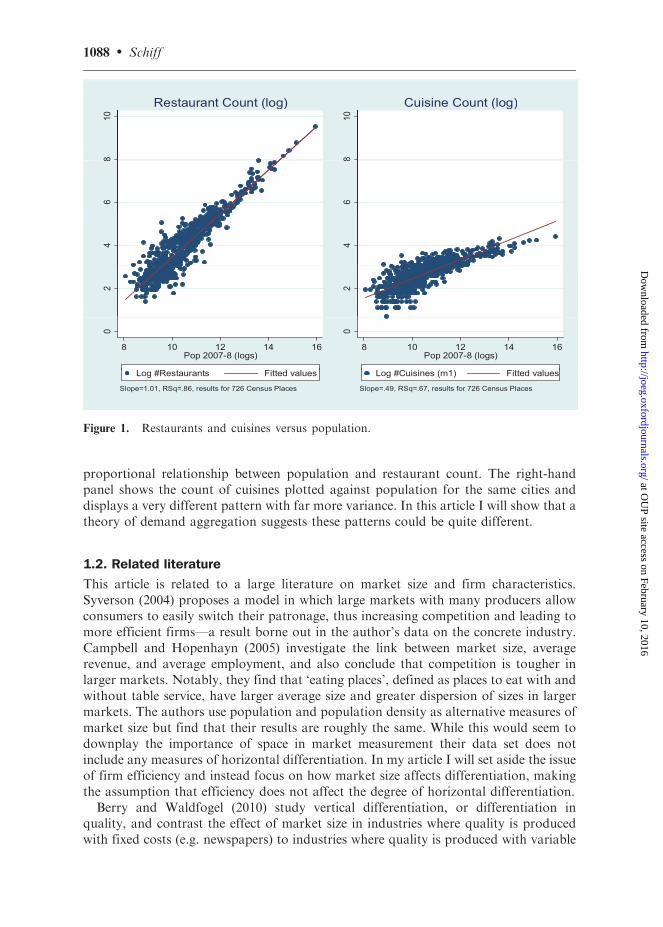
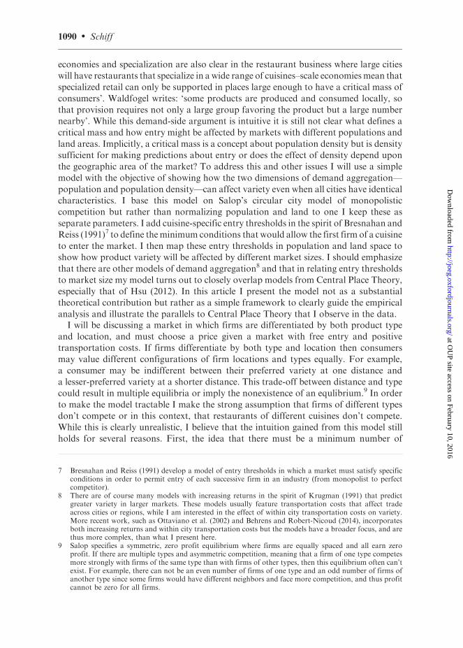
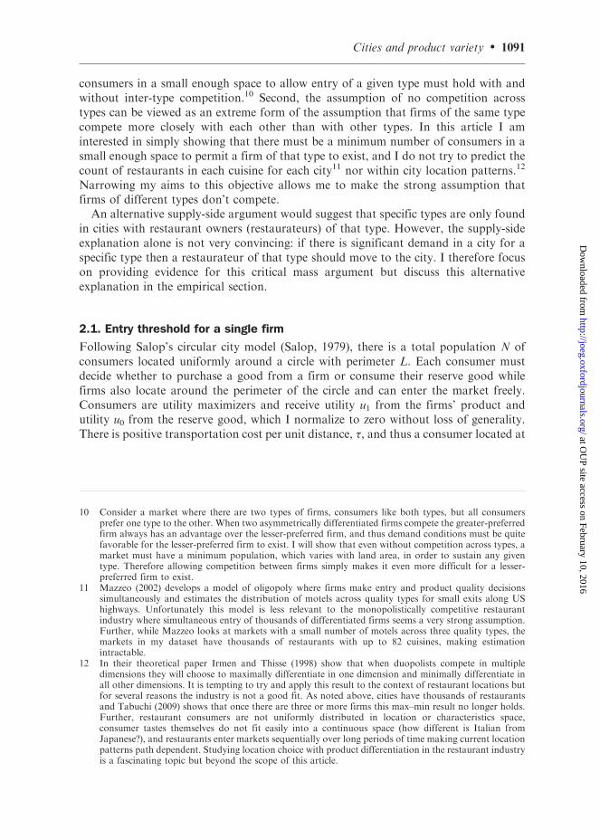
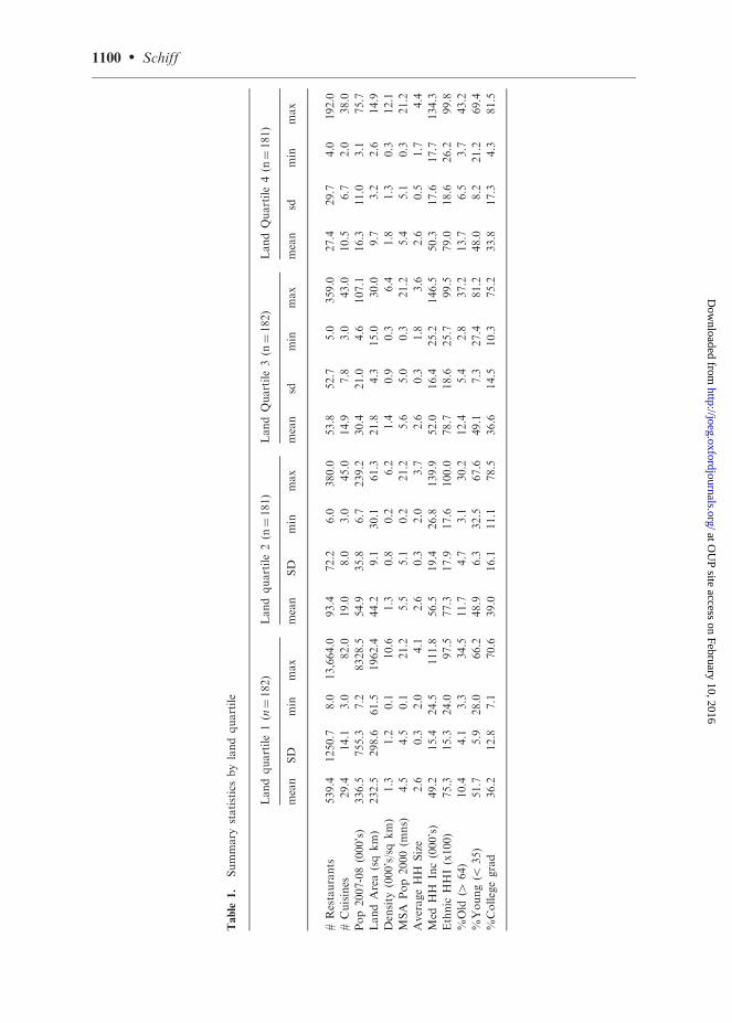
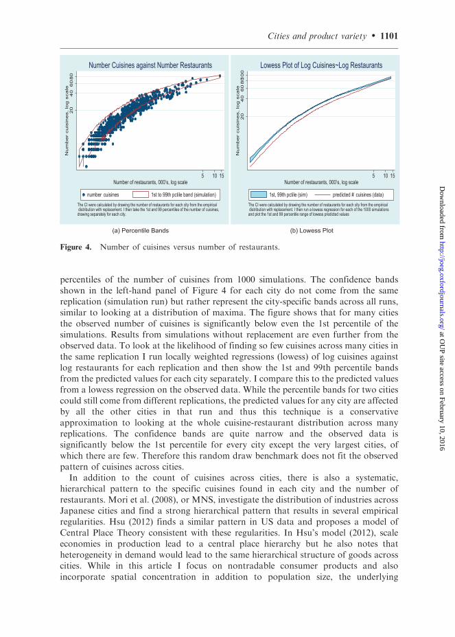
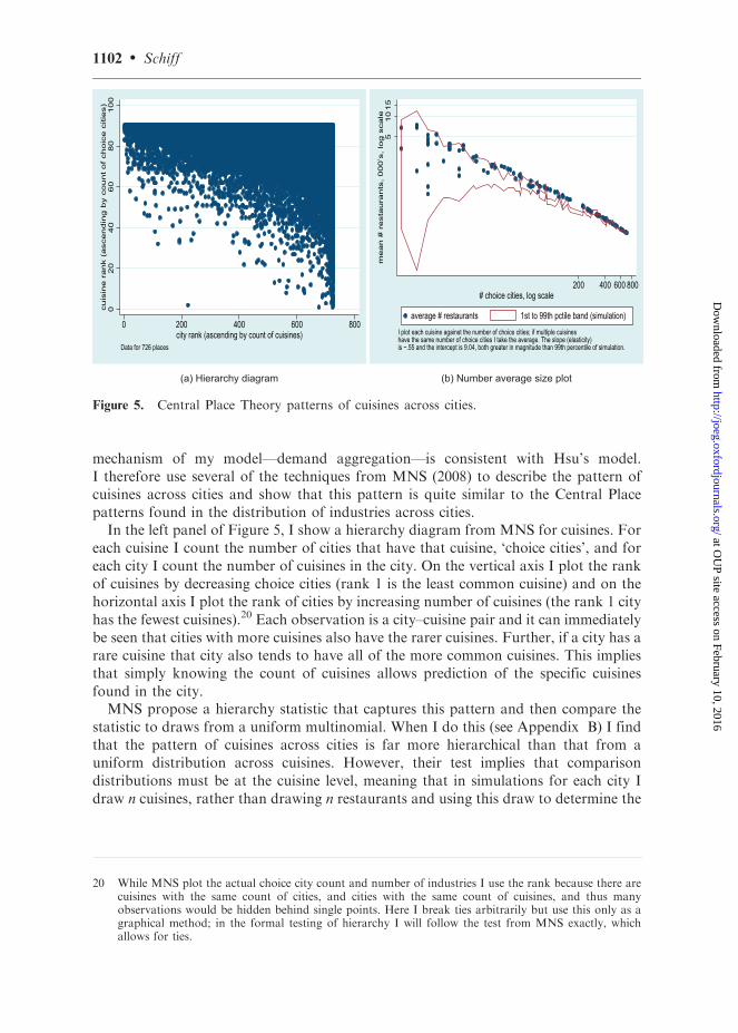
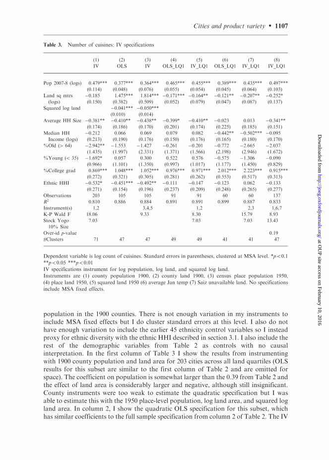
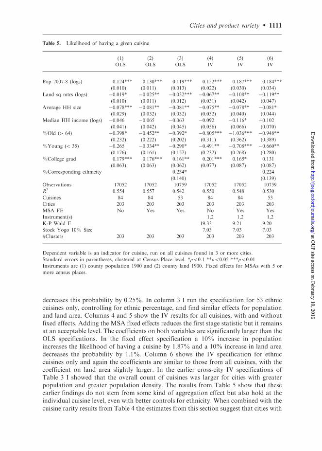
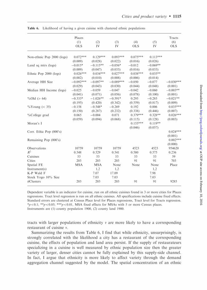
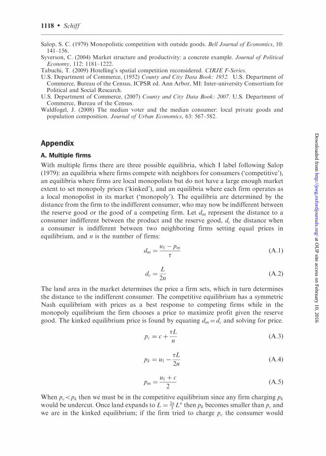
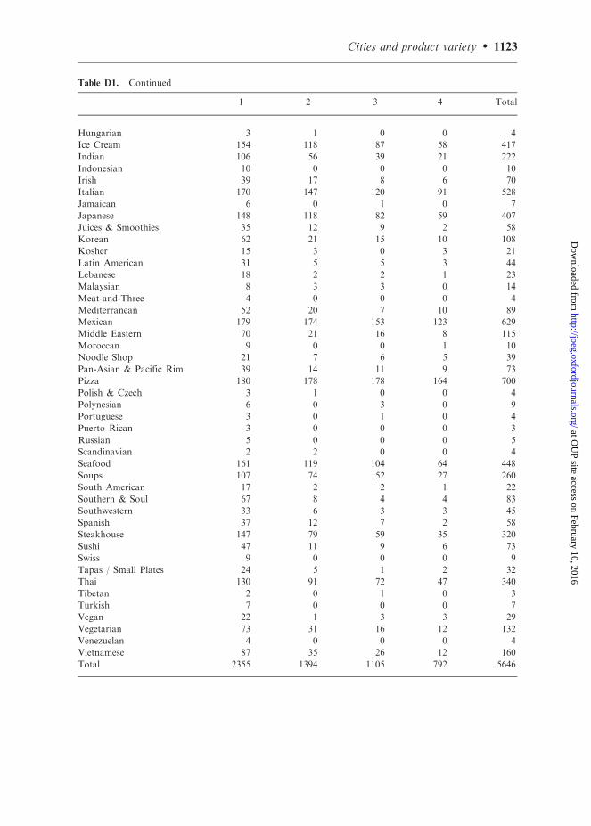

at OU
P site access on February 10 2016httpjoegoxfordjournalsorg
Dow
nloaded from

![[PPT]Evidence and Elaboration - Mrs. Wendorph's English ...wendorphela.weebly.com/.../evidence_and_elaboration.pptx · Web viewFinding Effective Evidence Include a variety of evidence](https://static.fdocuments.us/doc/165x107/5ae514227f8b9ae1578bd664/pptevidence-and-elaboration-mrs-wendorphs-english-viewfinding-effective.jpg)