CIRJE Discussion Papers can be downloaded without charge from:

http://www.e.u-tokyo.ac.jp/cirje/research/03research02dp.html

Discussion Papers are a series of manuscripts in their draft form. They are not intended for

circulation or distribution except as indicated by the author. For that reason Discussion Papers may

not be reproduced or distributed without the written consent of the author.

CIRJE-F-746

Efficient Bayesian Estimation of a MultivariateStochastic Volatility Model with Cross Leverage

and Heavy-Tailed Errors

Tsunehiro IshiharaGraduate School of Economics, University of Tokyo

Yasuhiro OmoriUniversity of Tokyo

May 2010

Efficient Bayesian estimation of a multivariate stochasticvolatility model with cross leverage and heavy-tailed

errors

Tsunehiro Ishiharaa, Yasuhiro Omori1,∗

aGraduate School of Economics, University of Tokyo, Japan.bFaculty of Economics, University of Tokyo, Bunkyo-Ku, Tokyo 113-0033, Japan.

Abstract

An efficient Bayesian estimation using a Markov chain Monte Carlo methodis proposed in the case of a multivariate stochastic volatility model as anatural extension of the univariate stochastic volatility model with leverageand heavy-tailed errors. Note that we further incorporate cross-leverageeffects among stock returns. Our method is based on a multi-move samplerthat samples a block of latent volatility vectors. The method is presentedas a multivariate stochastic volatility model with cross leverage and heavy-tailed errors. Its high sampling efficiency is shown using numerical examplesin comparison with a single-move sampler that samples one latent volatilityvector at a time, given other latent vectors and parameters. To illustrate themethod, empirical analyses are provided based on five-dimensional S&P500sector indices returns.

Keywords: Asymmetry, Heavy-tailed error, Leverage effect, Markov chainMonte Carlo, Multi-move sampler, Multivariate stochastic volatility

∗Corresponding author. Tel: +81-3-5841-5516. Email: omori@e.u-tokyo.ac.jp

May 30, 2010

1. Introduction

Univariate stochastic volatility (SV) models are well-known to success-fully account for time-varying variance in financial time series (Broto andRuiz (2004)). Many efficient Bayesian estimation methods that use Markovchain Monte Carlo (MCMC) methods are proposed, because the likelihoodfunctions are difficult to evaluate in the implementation of the maximumlikelihood estimation (e.g. Shephard and Pitt (1997), Omori et al. (2007)).

Extending these models to a multivariate SV (MSV) model has recentlybecome a major concern in the investigation of the correlation structure ofmultivariate financial time series, especially with regard to portfolio opti-mization, risk management, and derivative pricing. The multivariate factormodeling of stochastic volatilities has been widely introduced to describe thecomplex dynamic structure of high-dimensional stock returns data (Jacquieret al. (1999), Liesenfeld and Richard (2003), Pitt and Shephard (1999),Lopes and Carvalho (2007), and several efficient MCMC algorithms havebeen proposed (So and Choi (2009), Chib et al. (2006)). However, efficientestimation methods for MSV models with cross leverage (i.e., a non-zerocorrelation between the i-th asset return at time t and the j-th log volatilityat time t+1 for all i and j) or asymmetry have not been well investigated inthe literature except for simple bivariate models; see surveys by Asai et al.(2006) and Chib et al. (2009). Chan et al. (2006) considered the Bayesianestimation of MSV models in which correlations existed between measure-ment errors and state errors, but their framework did not address leverageeffects. Asai and McAleer (2006) simplified the MSV model with leverageby assuming no cross leverage effect (i.e., no correlation between the i-thasset return at time t and the j-th log volatility at time t+1 for i = j) andthus described a Monte Carlo likelihood estimation method.

In this paper, we consider a general MSV model with cross leverage andheavy-tailed errors and propose a novel and efficient MCMC algorithm usinga multi-move sampler that samples a block of latent volatility vectors simul-taneously. To the best of our knowledge, this is the first efficient multi-movesampler proposed in the literature for the general MSV model with crossleverage and heavy-tailed errors. In any MCMC implementation of the SVmodels, it is critical to efficiently sample the latent volatility (or state) vari-ables from their full conditional posterior distributions. The single-movesampler that draws a single volatility variable at a time given the othervolatility variables and parameters is easy to implement, but the resultingMCMC samples are known to have high autocorrelations. This implies thatwe must iterate the MCMC algorithm a large number of times in order to

2

obtain accurate estimates when using a single-move sampler. Thus, we pro-pose a fast and efficient state-sampling algorithm based on the approximatelinear and Gaussian state space model. Such a model is derived by approxi-mating the conditional likelihood function by a multivariate normal densityusing a Taylor expansion around the mode. Starting with the current sampleof state variables, the mode can be easily obtained by repeatedly applyingthe disturbance smoother (Koopman (1993)) to the approximate auxiliarystate space model. The samples from the posterior distribution of latentstate variables are obtained from the Metropolis-Hastings (MH) algorithmin which a simulation smoother for the linear and Gaussian state space mod-els (de Jong and Shephard (1995), Durbin and Koopman (2002)) is used togenerate a candidate variables.

The rest of the paper is organized as follows. Section 2 discusses theBayesian estimation of the MSV model using a multi-move sampler of latentstate variables. Extended models with heavy-tailed errors are also consid-ered. In Section 3, we provide numerical examples using simulation data,and show that our proposed method outperforms the simple single-movesampler with respect to sampling efficiencies. Section 4 provides empiricalanalyses based on five-dimensional stock return indices. Section 5 concludesthe paper.

2. The MSV model with cross leverage and heavy-tailed errors

2.1. MSV Model

Let yt denote a stock return at time t. The univariate SV model withleverage is given by

yt = exp(αt/2)εt, t = 1, . . . , n, (1)

αt+1 = ϕαt + ηt, t = 1, . . . , n− 1, (2)

and

α1 ∼ N (0, σ2η/(1− ϕ2)), (3)

where (εtηt

)∼ N2(0,Σ), Σ =

(σ2ε ρσεση

ρσεση σ2η

), (4)

αt is a latent variable for the log-volatility, and Nm(µ,Σ) denotes an m-variate normal distribution with mean µ and covariance matrix Σ. To

3

extend this model to the MSV model, let yt = (y1t, . . . , ypt)’ denote a p-dimensional stock returns vector, and let αt = (α1t, . . . , αpt)

′ denote thecorresponding log volatility vectors. We consider the MSV model given by

yt = V1/2t εt, t = 1, . . . , n, (5)

αt+1 = Φαt + ηt, t = 1, . . . , n− 1, (6)

and

α1 ∼ Np (0,Σ0) , (7)

where

Vt = diag (exp(α1t), . . . , exp(αpt)) , (8)

Φ = diag(ϕ1, . . . , ϕp), (9)

and (εtηt

)∼ N2p(0,Σ), Σ =

(Σεε Σεη

Σηε Σηη

). (10)

The (i, j)-th element of Σ0 is the (i, j)-th element of Σηη divided by 1−ϕiϕj

to satisfy the stationarity condition Σ0 = ΦΣ0Φ+Σηη such that

vec(Σ0) =(Ip2 −Φ⊗Φ

)−1vec(Σηη).

The expected value of the volatility evolution processes αt is set equal to0 for identifiability. Let θ = (ϕ,Σ), where ϕ = (ϕ1, . . . , ϕp)

′, and let 1pdenote a p × 1 vector with all elements equal to one. Then the likelihoodfunction of the MSV model outlined in equations (5) to (7) is given by

f(α1|θ)n−1∏t=1

f(yt,αt+1|αt,θ)f(yn|αn,θ)

∝ exp

{n∑

t=1

lt −1

2α′

1Σ−10 α1 −

1

2

n−1∑t=1

(αt+1 −Φαt)′Σ−1

ηη (αt+1 −Φαt)

}×|Σ0|−

12 |Σ|−

n−12 |Σεε|−

12 , (11)

4

where

lt = const− 1

21′pαt −

1

2(yt − µt)

′Σ−1t (yt − µt), (12)

µt = V1/2t mt, Σt = V

1/2t StV

1/2t , (13)

mt =

{ΣεηΣ

−1ηη (αt+1 − Φαt), t < n,

0 t = n,(14)

and

St =

{Σεε −ΣεηΣ

−1ηη Σηε, t < n,

Σεε t = n.(15)

2.2. Bayesian analysis and MCMC implementation

Since there are many latent volatility vectors αts, it is difficult to inte-grate them out in order to evaluate the likelihood function of θ analyticallyor to use high-dimensional numerical integration. In this paper, we take aBayesian approach and we employ a simulation method, namely, the MCMCmethod, to generate samples from the posterior distribution to conduct sta-tistical inference with respect to the model parameters.

For prior distributions of θ, we assume

ϕj + 1

2∼ B(aj , bj), j = 1, . . . , p, Σ ∼ IW(n0,R0),

where B(aj , bj) and IW(n0,R0) respectively denote Beta and inverse Wishartdistributions with probability density functions

π(ϕj) ∝ (1 + ϕj)aj−1 (1− ϕj)

bj−1 , j = 1, 2, . . . , p, (16)

π(Σ) ∝ |Σ|−n0+p+1

2 exp

{−1

2tr(R−1

0 Σ−1)}

. (17)

Using Equations (11), (16), and (17), we obtain the joint posterior densityfunction of (θ,α) given by

π(θ,α|Yn) ∝ f(α1|θ)n−1∏t=1

f(yt,αt+1|αt,θ)f(yn|αn,θ)

p∏j=1

π(ϕj)π(Σ), (18)

where α = (α′1, . . . ,α

′n)

′ and Yn = {yt}nt=1. We implement the MCMCalgorithm in three stages:

1. Generate α|ϕ,Σ, Yn.

5

2. Generate Σ|ϕ,α, Yn.

3. Generate ϕ|Σ,α, Yn.

First, we discuss two methods used to sample α based on its conditionalposterior distribution in Step 1. One method is a so-called single-movesampler that samples one αt at a time given the other αjs, while the othermethod is a multi-move sampler that samples a block of state vectors, suchas, (αt, . . . ,αt+k), given the other state vectors.

2.2.1. The generation of α

Single-move sampler. A simple but inefficient method is to sample oneαt at a time given αjs and other parameters. The conditional posteriorprobability density function of αt is

π(αt|{αs}s=t,ϕ,Σ, Yn) ∝ exp

{−1

2(αt −mαt)

′Σ−1αt

(αt −mαt) + g(αt)

}where

mαt =

Σα1

(−1

21p +ΦM1α2

), t = 1,

Σαt

(−1

21p +ΦMtαt+1 +Mt−1Φαt−1 +Nt−1

), 1 < t < n,

Σαn

(−1

21p +Mn−1Φαn−1 +Nn−1

), t = n,

Σαt =

(Σ−1

0 +ΦM1Φ)−1

, t = 1,

(Mt−1 +ΦMtΦ)−1 , 1 < t < n,

M−1n−1, t = n,

Mt = Σ−1ηη +Σ−1

ηη ΣηεS−1t ΣεηΣ

−1ηη , Nt = Σ−1

ηη ΣηεS−1t V

−1/2t yt,

and

g(αt) = −1

2y′tΣ

−1t yt + y′

tΣ−1t µt.

Thus, in order to sample from the conditional posterior distribution usingthe Metropolis-Hastings (MH) algorithm, we generate a candidate α†

t ∼N(mαt ,Σαt) and accept it with probability

min{exp{g(α†

t)− g(αt)}, 1},

for t = 1, . . . , n, where αt is a current value.

Multi-move sampler. As an alternative method, we propose an efficient

6

method to sample a block of αts from the posterior distribution. As such,we extend Omori and Watanabe (2008), who considered the univariate SVmodel with leverage (see also Takahashi et al. (2009)). First, we divide α =(α′

1, . . . ,α′n)

′ into K + 1 blocks (α′ki−1+1, . . . ,α

′ki)′ using i = 1, . . . ,K + 1,

with k0 = 0, kK+1 = n, and ki − ki−1 ≥ 2. K knots (k1, . . . , kK) aregenerated randomly using

ki = int[n× (i+ Ui)/(K + 2)], i = 1, . . . ,K,

where Uis are independent uniform random variables on (0, 1) (Shephardand Pitt (1997)). These stochastic knots have an advantage in that theyallow the points of conditioning to change over the MCMC iterations, as Kis a tuning parameter used to obtain MCMC samples with relatively lowautocorrelation.

Suppose that ki−1 = s and ki = s+m for the i-th block. Consider sam-pling this block from its conditional posterior distribution given other statevectors and parameters. We denote xt = R−1

t ηt, where the matrix Rt de-notes a Choleski decomposition ofΣηη = RtR

′t for t > 0, andΣ0 = R0R

′0 for

t = 0. To construct a proposal distribution for the MH algorithm, we focuson the distribution of the disturbance x ≡ (x′

s, . . . ,x′s+m−1)

′, which is funda-mental in the sense that it derives the distribution of a ≡ (α′

s+1, . . . ,α′s+m)′.

Then, the logarithm of the full conditional joint density distribution of x,excluding constant terms, is given by

log f(x|αs,αs+m+1,ys, . . . ,ys+m) = −1

2

s+m−1∑t=s

x′sxs + L, (19)

where

L =s+m∑t=s

ls −1

2(αs+m+1 −Φαs+m)′Σ−1

ηη (αs+m+1 −Φαs+m)I(s+m < n).

Using the second order Taylor expansion of (19) around the mode x, weobtain the approximate normal density f∗, which is used for the Acceptance-Rejection MH(ARMH) algorithm as follows.

7

log f(x|αs,αs+m+1,ys, . . . ,ys+m)

≈ const.− 1

2

s+m−1∑t=s

x′txt + L

+∂L

∂x′

∣∣∣∣∣x=x

(x− x) +1

2(x− x)′E

(∂2L

∂x∂x′

)(x− x)

= const.− 1

2

s+m−1∑t=s

x′txt + L+ d′(a− a)− 1

2(a− a)′Q(a− a) (20)

= const. + log f∗(x|αs,αs+m+1,ys, . . . ,ys+m), (21)

where Q and d are Q = −E(∂2L/∂a∂a′), and d = ∂L/∂a, is evaluatedat a = a (i.e., x = x). Note that Q is positive definite and invertible.However, whenm is large, it is time consuming to invert themp×mp Hessianmatrix to obtain the covariance matrix of themp-variate multivariate normaldistribution. To overcome this difficulty, we interpret equation (21) as theposterior probability density derived from an auxiliary state space model sothat we only need to invert p×p matrices by using the Kalman filter and thedisturbance smoother. It can be shown that f∗ is the posterior probabilitydensity function of x obtained from the state space model:

yt = Ztαt +Gtut, t = s+ 1, . . . , s+m, (22)

αt+1 = Φαt +Htut, t = s+ 1, . . . , s+m− 1, (23)

where ut ∼ N2p (0, I2p), yt, Zt, and Gt are defined in Appendix A.1, andHt = [0,Rt]. To find a mode x, we repeat the following three steps untilthe convergence,

1. Compute a at x = x using (6).

2. Obtain the approximate linear Gaussian state space model given by(22) and (23).

3. Applying the disturbance smoother by Koopman (1993) to the ap-proximating linear Gaussian state space model in Step 2, compute theposterior mode x.

Note that these steps are equivalent to the method of scoring used to max-imize the conditional posterior density. As an initial value of x, the currentsample of x may be used in MCMC implementation. If the approximate lin-ear Gaussian state space model is obtained using mode x, we draw a sample

8

x from the conditional posterior distribution by the AR-MH algorithm asfollows.

1. Propose a candidate x† by sampling from q(x†) ∝ min(f(x†), cf∗(x†))using the AR algorithm, where c can be constructed from a constantterm and L from (20).

(a) Generate x† ∼ f∗ using a simulation smoother (de Jong andShephard (1995), Durbin and Koopman (2002)) based on theapproximate linear Gaussian state space model in (22) and (23).

(b) Accept x† with probability min{

f(x†)cf∗(x†)

, 1}. If it is rejected, re-

turn to (a).

2. Given the current value x, accept x† with probability

min

{1,

f(x†)min(f(x), cf∗(x))

f(x)min(f(x†), cf∗(x†))

}.

If rejected, accept the current x as a sample.

We investigate the efficiency performance of these two sampling methods inSection 3 using simulated data.

2.2.2. The generation of Σ and ϕ

Generation of Σ. The conditional posterior probability density function ofΣ is

π(Σ|ϕ,α, Yn) ∝ |Σ|−n1+2p+1

2 exp

{−1

2tr(R−1

1 Σ−1)}

× g(Σ),

g(Σ) = |Σ0|−12 |Σεε|−

12 exp

{−1

2

(α′

1Σ−10 α1 + y′

nV−1/2n Σ−1

εε V−1/2n yn

)},

where n1 = n0 + n− 1, R−11 = R−1

0 +∑n−1

t=1 vtv′t and

vt =

(V

−1/2t yt

αt+1 −Φαt

).

Using the MH algorithm, we propose a candidate Σ† ∼ IW(n1,R1) andaccept it with probability min{g(Σ†)/g(Σ), 1} where Σ is a current sample.

Generation of ϕ. Let Σij be a p × p matrix, and denote the (i, j)-th block

of Σ−1. Furthermore, let A =∑n−1

t=1 αtα′t, B =

∑n−1t=1 {αty

′tV

−1/2t Σ12 +

9

αtα′t+1Σ

22}, and b denote a vector for which the i-th element is equal tothe (i, i)-th element of B. Then the conditional posterior probability densityfunction of ϕ is

π(ϕ|Σ,α, Yn) ∝ h(ϕ)× exp

{−1

2tr(ΦΣ22ΦA)− 2tr(ΦB)

}∝ h(ϕ)× exp

{−1

2(ϕ− µϕ)

′Σϕ(ϕ− µϕ)

},

h(ϕ) = |Σ0|−12

p∏j=1

(1 + ϕj)aj−1(1− ϕj)

bj−1 exp

{−1

2α′

1Σ−10 α1

},

where µϕ = Σϕb, Σ−1ϕ = Σ22 ⊙ A, and ⊙ denotes a Hadamard product.

To sample ϕ based on its conditional posterior distribution using the MHalgorithm, we generate a candidate from a truncated normal distributionover the region R, ϕ† ∼ T NR(µϕ,Σϕ), and R = {ϕ : |ϕj | < 1, j = 1, . . . , p}and accept it with probability min{h(ϕ†)/h(ϕ), 1} where ϕ is a currentsample.

2.3. The associated particle filter

This subsection describes the auxiliary particle filter (Pitt and Shephard(1999)) used to compute the likelihood function ordinate given the parameterθ, which can be used for model comparison. For more detail on the auxiliaryparticle filter, see Doucet et al. (2001).

Let f(αt|Yt,θ) denote the conditional probability density function of αt

given (Yt,θ), and let f(αt|Yt,θ) denote the corresponding discrete proba-bility mass function that approximates f(αt|Yt,θ). We consider samplingfrom the conditional joint distribution of (αt+1,αt) given (Yt+1,θ), with aprobability density function given by

f(αt+1,αt|Yt+1,θ) ∝ f(yt+1|αt+1)f(αt+1|yt,αt,θ)f(αt|Yt,θ), (24)

where

f(yt|αt) =

(2π)−p/2 |V1/2t ΣεεV

1/2t |−1/2 exp

{−1

2y′tV

−1/2t Σ−1

εε V−1/2t yt

}, (25)

f(αt+1|yt,αt,θ) =

(2π)−p/2 |Σα|−1/2 exp

{−1

2(αt+1 − µα,t+1)

′Σ−1α (αt+1 − µα,t+1)

}, (26)

10

and

µα,t+1 = Φαt +ΣηεΣ−1εε V

−1/2t yt, Σα = Σηη −ΣηεΣ

−1εε Σεη. (27)

We use the importance probability density function given by

g(αt+1,αit|Yt+1,θ) ∝ f(yt+1|µi

α,t+1)f(αt+1|yt,αit,θ)f(α

it|Yt,θ)

∝ f(αt+1|yt,αit,θ)g(α

it|Yt+1,θ),

where

g(αit|Yt+1,θ) =

f(yt+1|µiα,t+1)f(α

it|Yt,θ)∑I

i=1 f(yt+1|µiα,t+1)f(α

it|Yt,θ)

,

µiα,t+1 = Φαi

t +ΣηεΣ−1εε V

i −1/2t yt, Vi

t = Vt|αt=αit.

We derive the auxiliary particle filter as follows:

Step 1. Initialize t = 1, and generate αi1 ∼ N (0,Σ0), (i = 1, . . . , I).

(a) Compute wi = f(y1|αi1,θ), and record w1 =

1I

∑Ii=1wi.

(b) Let f(αi1|Y1,θ) = πi

1 = wi/∑I

j=1wj , (i = 1, . . . , I).

Step 2.

(a) For each i, generate(αi

t+1,αit

)from g(αt+1,α

jt |Yt+1,θ), (i, j =

1, . . . , I), as follows. First, resample αit, i = 1, . . . , I, with prob-

ability g(αjt |Yt+1,θ), j = 1, . . . , I. Then generate αi

t+1, i =1, . . . , I, from the normal distribution with density function f(αt+1|yt,α

it,θ).

(b) Compute

wi =f(yt+1|αi

t+1)f(αit+1|yt,α

it,θ)f(α

it|Yt,θ)

g(αi

t+1,αit|Yt+1,θ

)=

f(yt+1|αit+1)f(α

it|Yt,θ)

g(αit|Yt+1,θ)

,

for i = 1, . . . , I, and record wt =∑I

i=1wi/I.

(c) Let f(αit+1|Yt+1,θ) = πi

t+1 = wi/∑I

j=1wj (i = 1, . . . , I).

Step 3 Increase t by one and return to Step 2.

Then,n∑

t=1

logwtp→

n∑t=1

log f(yt|Yt−1,θ), as I → ∞,

is a consistent estimate of the conditional log-likelihood.

11

2.4. The extension of the MSV model with multivariate-t errors (MSVtmodel)

The MSV model can be extended to incorporate heavy-tailed errors instock returns. Although jump components can also be introduced, they arenot considered here for the reasons of simplicity. To describe the fat-taileddistributions, we consider the multivariate-t distribution, which is a scalemixture of normal distributions. Let G(a, b) denote a gamma distributionwith mean a/b and variance a/b2. Using a common scalar gamma randomvariable λt, the multivariate-t random variable with ν degrees of freedom isobtained as

λ−1/2t εt, where λt ∼ G(ν/2, ν/2), εt ∼ Np(0,Σεε). (28)

Thus, we extend the MSV model to a MSV multivariate-t errors (MSVt)model, where the measurement equation is given by

yt = λ−1/2t V

1/2t εt, (29)

for t = 1, . . . , n. The prior distribution for ν is assumed to be ν ∼ G(mν0 , S

ν0 ),

and we let π(ν) denote its prior probability density function.To implement MCMC simulation, we sample (α,ϕ,Σ) as in Section

2.2, but we replace yt with λ1/2t yt. Thus, we focus on sampling from the

conditional posterior distributions for the other parameters (ν,λ) whereλ = {λt}nt=1. Their conditional joint posterior probability density functionis given by

π(ν,λ|ϕ,Σ,α, Yn)

∝ π(ν)

{(ν2

) ν2

Γ(ν2

)}n n∏t=1

λp+ν2

−1t

× exp

[−1

2

n∑t=1

{νλt +

(√λtyt − µt

)′Σ−1

t

(√λtyt − µt

)}]. (30)

To sample from the posterior distribution, we implement the MCMC simu-lation in three blocks.

1. Generate (α,ϕ,Σ) as in Section 2.2.1, replacing yt with λ1/2t yt.

2. Generate ν ∼ π(ν|λ).

12

3. Generate λt ∼ π(λt|ϕ,Σ,αt, ν,yt) for t = 1, . . . , n.

Generation of ν. The conditional posterior probability density of ν is givenby

π(ν|ϕ,Σ,λ,α, Yn) ∝ π(ν)

{(ν2

) ν2

Γ(ν2

)}n( n∏t=1

λt

) ν2

exp

{−∑n

t=1 λt

2ν

}. (31)

To sample from this conditional posterior distribution, we transform ν suchthat ϑν = log ν and we let ϑν denote a conditional mode of π(ϑν |ϕ,Σ,λ,α, Yn).Using the MH algorithm, we propose a candidate from the normal distribu-tion ϑ†

ν ∼ N (µν , σ2ν), where

µν = ϑν + σ2ν

[∂ log π(ϑν |ϕ,Σ,λ,α, Yn)

∂ϑν

∣∣∣∣ϑν=ϑν

],

and

σ2ν =

[−∂2 log π(ϑν |ϕ,Σ,λ,α, Yn)

∂ϑ2ν

∣∣∣∣ϑν=ϑν

]−1

.

We accept the candidate with probability

min

[π(ϑ†

ν |ϕ,Σ,λ,α, Yn)fN (ϑν |µν , σ2ν)

π(ϑν |ϕ,Σ,λ,α, Yn)fN (ϑ†ν |µν , σ2

ν), 1

],

where ϑν is a current sample, and fN (x|µ, σ2) denotes a probability densityfunction derived from a normal distribution with mean µ and variance σ2.

Generation of λ. The conditional posterior probability density function ofλt is

π(λt|ϕ,Σ, ν,α, Yn) ∝ λν+p2

−1t exp

{−ct

2λt + dt

√λt

},

where ct = ν + y′tΣ

−1t yt, and dt = y′

tΣ−1t µt. To sample λt using the MH

algorithm, we generate a candidate λ†t ∼ G((ν + p)/2, ct/2) and accept it

13

with probability,

min

[1, exp

{dt

(√λ†t −

√λt

)}],

where λt is a current sample. Note that we generate λn ∼ G((ν+p)/2, cn/2),since µn = 0 implies dn = 0.

3. Illustrative examples using simulated data

This section illustrates our proposed method using simulated data andshows the efficiency of our proposed multi-move sampler in comparison withthe single-move sampler. The data are simulated using the MSVt modelpresented in Section 2.4, with

ϕi = 0.97, σi,εε ≡√

V ar(εit) = 1.2, σi,ηη ≡√V ar(ηit) = 0.2,

ρi,εη ≡ Corr(εit, ηit) = −0.4, ν = 15, i = 1, 2, . . . , 5,

which correspond to typical values for the parameters of the univariate SVmodels in past empirical studies. The negative value of ρi,εη implies theexistence of leverage effects. For the correlations among εits and ηjts, we setsimilar values to those obtained in our empirical studies.

ρij,εε ≡ Corr(εit, εjt) = 0.6, ρij,ηη ≡ Corr(ηit, ηjt) = 0.7,

ρij,εη ≡ Corr(εit, ηjt) = −0.3, for i = j,

where the negative value of ρij,εη indicates cross leverage effects. Usingthese parameters, we generated n = 4, 000 observations with p = 5. Forprior distributions, we assume

ϕi + 1

2∼ B(20, 1.5), Σ ∼ IW(10, (10Σ∗)−1), ν ∼ G(1, 0.05),

where Σ∗ is a true covariance matrix so that E(Σ−1) = Σ∗−1. The meanand standard deviation of the prior distribution of ϕj are set 0.86 and 0.11respectively, while the mean and standard deviation of ν are set 20 and 20,respectively. Using the MCMC algorithm described in Section 2.2, we gen-erated 120,000 samples using the multi-move sampler and 550,000 samplesusing the single-move sampler, discarding the first 20,000 and 50,000 sam-ples as burn-in periods, respectively.

14

Estimation results. Tables 1 and 2 show the estimation results using themulti-move sampler with tuning parameterK = 200 for (ϕi, σi,εε, σi,ηη, ρi,εη, ν)and (ρij,εε, ρij,ηη, ρij,εη), respectively. The results using the single-move sam-pler are omitted, except the inefficiency factors (shown in the brackets inTable 1), since they are similar to those obtained for the multi-move sampler.The posterior means and 95% credible intervals suggest that the estimatesare sufficiently close to true values, which indicates that our proposed esti-mation algorithm works well.

The inefficiency factor is defined as 1+2∑∞

s=1 ρs, where ρs is the sampleautocorrelation at lag s; this factor is computed to measure how well theMCMC mixes (Chib (2001)). It is the ratio of the numerical variance ofthe posterior sample mean to the variance of the sample mean based onuncorrelated draws. When the inefficiency factor is equal to m, we mustdraw m times as many as the number of uncorrelated samples.

Table 1: Estimation results for ϕi, σi,εε, σi,ηη, ρi,εη and ν.

Posterior means, 95% credible intervals, and inefficiency factors.

True i Mean 95% interval Inefficiencymulti [single]

ϕi 0.97

1 0.965 [0.956, 0.973] 79 [786]2 0.973 [0.965, 0.980] 79 [624]3 0.971 [0.963, 0.978] 78 [298]4 0.964 [0.954, 0.972] 58 [563]5 0.969 [0.960, 0.977] 111 [449]

σi,εε 1.2

1 1.191 [1.093, 1.297] 180 [4083]2 1.177 [1.068, 1.304] 236 [6732]3 1.195 [1.089, 1.310] 210 [6327]4 1.261 [1.163, 1.370] 163 [2830]5 1.187 [1.081, 1.300] 198 [4450]

σi,ηη 0.2

1 0.207 [0.181, 0.235] 128 [827]2 0.192 [0.168, 0.218] 152 [788]3 0.189 [0.167, 0.214] 136 [448]4 0.208 [0.182, 0.236] 132 [901]5 0.209 [0.183, 0.236] 181 [676]

ρi,εη −0.4

1 -0.412 [-0.503,-0.316] 58 [294]2 -0.400 [-0.496,-0.298] 62 [266]3 -0.335 [-0.438,-0.226] 62 [297]4 -0.377 [-0.476,-0.275] 42 [221]5 -0.396 [-0.490,-0.296] 81 [253]

ν 15 15.7 [13.0,19.1] 48 [151]

15

Table 2: Estimation results for ρij,εε, ρij,ηη and ρij,εη.

Posterior means, 95% credible intervals and inefficiency factors.

True ij Mean 95% interval Inefficiencymulti [single]

ρij,εε 0.6

12 0.596 [0.574, 0.617] 3 [16]13 0.606 [0.585, 0.627] 2 [18]14 0.610 [0.589, 0.631] 2 [13]15 0.586 [0.564, 0.608] 2 [18]23 0.582 [0.559, 0.603] 3 [21]31 0.586 [0.564, 0.608] 3 [27]32 0.597 [0.575, 0.618] 3 [20]34 0.599 [0.577, 0.620] 3 [27]35 0.590 [0.567, 0.611] 3 [24]45 0.607 [0.585, 0.628] 3 [24]

ρij,ηη 0.7

12 0.693 [0.599, 0.776] 114 [473]13 0.677 [0.575, 0.765] 81 [724]14 0.692 [0.592, 0.777] 115 [726]15 0.727 [0.637, 0.800] 137 [686]23 0.676 [0.576, 0.760] 113 [794]31 0.645 [0.531, 0.738] 115 [676]32 0.648 [0.543, 0.739] 119 [611]34 0.659 [0.554, 0.749] 147 [882]35 0.749 [0.656, 0.825] 160 [937]45 0.635 [0.529, 0.729] 106 [527]

ρij,εη −0.3

12 -0.282 [-0.389,-0.170] 60 [279]13 -0.242 [-0.351,-0.129] 68 [248]14 -0.297 [-0.399,-0.190] 48 [236]15 -0.253 [-0.357,-0.148] 57 [432]21 -0.275 [-0.370,-0.174] 55 [195]23 -0.273 [-0.377,-0.165] 66 [209]24 -0.281 [-0.382,-0.176] 41 [217]25 -0.229 [-0.330,-0.127] 74 [509]31 -0.316 [-0.412,-0.214] 43 [250]32 -0.264 [-0.372,-0.152] 74 [227]34 -0.262 [-0.365,-0.155] 37 [268]35 -0.237 [-0.343,-0.129] 52 [462]41 -0.337 [-0.434,-0.236] 49 [254]42 -0.368 [-0.467,-0.261] 57 [282]43 -0.289 [-0.395,-0.178] 68 [254]45 -0.237 [-0.340,-0.131] 61 [455]51 -0.382 [-0.477,-0.283] 47 [204]52 -0.352 [-0.457,-0.244] 67 [241]53 -0.372 [-0.481,-0.263] 90 [190]54 -0.280 [-0.386,-0.174] 47 [218]

16

As shown in Table 1, the inefficiency factors for the parameters obtainedfrom the single-move sampler are much larger than those from the multi-move sampler. Especially, for σi,εε, they are about 20 to 30 times larger forthe single-move sampler. This implies that our multi-move sampler is highlyefficient, as expected.

0 200 400 600 800 10000.00

0.25

0.50

0.75

1.00 Multi−move samplerσ22,εε

0 200 400 600 800 1000

0.25

0.50

0.75

1.00 Single−move samplerσ22,εε

0 20000 40000 60000 80000 100000

1.1

1.2

1.3

1.4 σ22,εε

0 20000 40000 60000 80000 100000

1.1

1.2

1.3

1.4 σ22,εε

Figure 1: Sample autocorrelation functions and paths of σ2,εε:

Single-move sampler versus Multi-move sampler.

Furthermore, for σ2,εε, Figure 1 shows the sample autocorrelation func-tions and the sample paths for the single-move and the multi-move samplers.In contrast with the very slow decay of the sample autocorrelations in thesingle-move sampler, these autocorrelations vanish fairly rapidly under themulti-move sampler. Further, the sample path of the single-move samplershows relatively slow movement in state space. This also indicates that theMCMC mixes well under the multi-move sampler.

Table 3: Maximum of inefficiency factors for K = 50, 100, 140, 200, and 270

K n/(K + 1) ϕj σi,εε σi,ηη ρi,εη ρij,εε ρij,ηη ρij,εη ν50 79 221 407 388 168 8 323 163 152100 40 153 160 256 84 4 219 101 66140 29 151 242 214 86 4 185 100 29200 20 111 236 181 81 3 160 90 48270 15 92 257 154 69 3 155 73 46

single-move 1 786 6732 901 297 27 937 509 151

17

Selection of a tuning parameter K. We set K = 200 in this example asfollows. Table 3 shows the maxima of inefficiency factors for ϕjs, σi,εεs,σi,ηηs, ρi,εηs, ρij,εεs, ρij,ηηs, ρij,εηs, and ν using K = 50, 100, 140, 200, and270. Since the maxima for K = 200 are overall smaller than those for otherKs, this is selected as an optimal value in our MCMC simulation. If thisvalue is greater than 200 (i.e., the number of elements in one block becomessmall on an average), the Markov chain would not move quickly in statespace due to high correlations among adjacent αts. However, if K is lessthan 200, the proposed states, namely, αts, would be rejected too often inthe MH algorithm, which also results in the slowed mixing of the chain.

4. Empirical studies

4.1. Data

19951997 1999 2001 2003 2005 2007 2009

−10

0

Materials

19951997 1999 2001 2003 2005 2007 2009

−10

0

10

20Financials

19951997 1999 2001 2003 2005 2007 2009

−5

0

Consumer Staples

19951997 1999 2001 2003 2005 2007 2009

−5

0

5Healthcare

19951997 1999 2001 2003 2005 2007 2009

−5

0

Utilities

19951997 1999 2001 2003 2005 2007 2009

−5

0

5S&P500

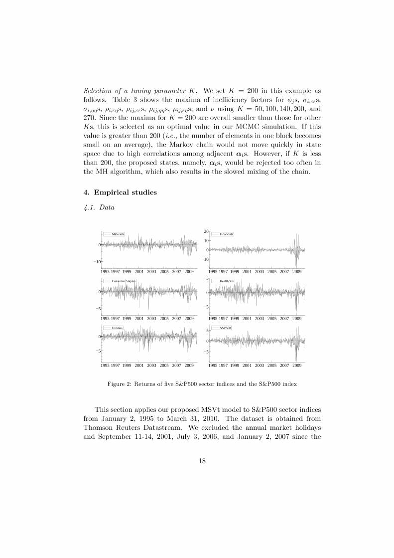
Figure 2: Returns of five S&P500 sector indices and the S&P500 index

This section applies our proposed MSVt model to S&P500 sector indicesfrom January 2, 1995 to March 31, 2010. The dataset is obtained fromThomson Reuters Datastream. We excluded the annual market holidaysand September 11-14, 2001, July 3, 2006, and January 2, 2007 since the

18

same value is recorded on those days as the value from the previous day.The returns are defined by the log-difference of each sector index multipliedby 100 for five series, namely, ‘Materials’ (Series 1), ‘Financials’ (Series 2),‘Consumer Staples’ (Series 3), ‘Healthcare’ (Series 4), and ‘Utilities’ (Series5). There are 3,839 trading days, and the time series plot of the five returnseries with S&P500 index returns are shown in Figure 2, which indicates theco-movement of volatility among the five stock returns during this period.

Table 4: Univariate SV model with leverage and t-distributed errors.

Posterior means, standard deviations, and 95% credible intervals.

Param. Series Mean Stdev 95% interval

ϕi

1 0.989 0.003 [0.983, 0.994]2 0.991 0.002 [0.987, 0.995]3 0.984 0.003 [0.977, 0.989]4 0.985 0.003 [0.978, 0.991]5 0.984 0.004 [0.977, 0.991]

σi,εε

1 1.248 0.102 [1.067, 1.472]2 1.415 0.150 [1.142, 1.728]3 0.871 0.055 [0.765, 0.983]4 1.051 0.074 [0.919, 1.210]5 0.976 0.077 [0.843, 1.146]

σi,ηη

1 0.124 0.012 [0.101, 0.150]2 0.143 0.012 [0.121, 0.167]3 0.148 0.013 [0.124, 0.174]4 0.144 0.014 [0.118, 0.175]5 0.151 0.014 [0.126, 0.182]

ρi,εη

1 -0.527 0.065 [-0.644,-0.393]2 -0.684 0.049 [-0.771,-0.579]3 -0.608 0.056 [-0.707,-0.489]4 -0.568 0.060 [-0.678,-0.443]5 -0.346 0.070 [-0.482,-0.208]

νi

1 22.7 11.3 [12.1, 55.9]2 25.0 15.4 [12.8, 69.8]3 25.5 12.6 [13.0, 59.0]4 16.5 5.2 [10.1, 28.7]5 46.5 27.6 [16.4,115.3]

4.2. The univariate SV model with leverage and t-distributed errors

First, we fit the univariate SV model with leverage and t-distributederrors to individual series as a benchmark for the MSVt model. The prior

19

distributions for ϕ and Σ are assumed to be

ϕi + 1

2∼ B(20, 1.5), νi ∼ G(0.01, 0.01),

Σi ∼ IW(5, (5Σ∗i )

−1), Σ∗i =

(1 −0.1

−0.1 0.04

),

for i = 1, . . . , 5, where νi is the degrees of freedom for the respective t-distribution. Since the posterior estimates of νi may be sensitive to thechoice of the prior distribution (Nakajima and Omori (2009)), we use arelatively flat prior. To implement the MCMC algorithm, we draw 60,000samples and discard 10,000 samples as a burn-in period. Posterior means,standard deviations, and 95% credible intervals are shown in Table 4.

The estimates of ϕi show the high persistence of log volatilities varyingfrom 0.984 to 0.991; those negative values of ρi (ranging from −0.684 to−0.346) imply the credible existence of leverage effects for all series. Fur-thermore, the degrees of freedoms ν are relatively small (16.5 to 46.5) whichindicate distributions with heavy-tails. These results are consistent withthose found in previous empirical studies.

4.3. The MSVt model

For the MSVt model, the prior distributions are assumed to be

ϕi + 1

2∼ B(20, 1.5), i = 1, . . . , 5,

Σ ∼ IW(10, (10Σ∗)−1), ν ∼ G(0.01, 0.01),

where

Σ∗ =

(Σ∗

εε Σ∗εη

Σ∗′εη Σ∗

ηη

)=

(1.22(0.5I5 + 0.5151

′5) 1.2× 0.2× (−0.1)I5

0.22(0.2I5 + 0.8151′5)

),

and E(Σ−1) = Σ∗−1. Hyper-parameters of the prior distributions are chosenbased on an analysis of univariate SV models. Using the MCMC algorithmsdescribed in Section 2, we draw 100,000 samples after discarding 20,000samples as a burn-in period. The tuning parameter K is set to 100 basedon an analysis similar to that presented in Table 3. This means that theaverage size of one block is about 40.

20

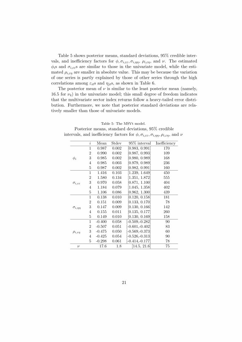
Table 5 shows posterior means, standard deviations, 95% credible inter-vals, and inefficiency factors for ϕ, σi,εε, σi,ηη, ρi,εη, and ν. The estimatedϕis and σi,εεs are similar to those in the univariate model, while the esti-mated ρi,εη are smaller in absolute value. This may be because the variationof one series is partly explained by those of other series through the highcorrelations among εits and ηjts, as shown in Table 6.

The posterior mean of ν is similar to the least posterior mean (namely,16.5 for ν4) in the univariate model; this small degree of freedom indicatesthat the multivariate sector index returns follow a heavy-tailed error distri-bution. Furthermore, we note that posterior standard deviations are rela-tively smaller than those of univariate models.

Table 5: The MSVt model.

Posterior means, standard deviations, 95% credibleintervals, and inefficiency factors for ϕ, σi,εε, σi,ηη, ρi,εη, and ν

i Mean Stdev 95% interval Inefficiency

ϕi

1 0.987 0.002 [0.983, 0.991] 1702 0.990 0.002 [0.987, 0.993] 1093 0.985 0.002 [0.980, 0.989] 1684 0.985 0.003 [0.979, 0.989] 2365 0.987 0.002 [0.982, 0.991] 160

σi,εε

1 1.416 0.103 [1.239, 1.649] 4502 1.580 0.134 [1.351, 1.872] 5553 0.970 0.058 [0.871, 1.100] 4044 1.184 0.079 [1.045, 1.358] 4025 1.106 0.086 [0.962, 1.300] 439

σi,ηη

1 0.138 0.010 [0.120, 0.158] 1812 0.151 0.009 [0.133, 0.170] 783 0.147 0.009 [0.130, 0.166] 1424 0.155 0.011 [0.135, 0.177] 2605 0.149 0.010 [0.130, 0.169] 158

ρi,εη

1 -0.400 0.058 [-0.509,-0.282] 902 -0.507 0.051 [-0.601,-0.402] 833 -0.475 0.050 [-0.569,-0.373] 604 -0.425 0.054 [-0.526,-0.313] 905 -0.298 0.061 [-0.414,-0.177] 78

ν 17.6 1.8 [14.5, 21.6] 75

21

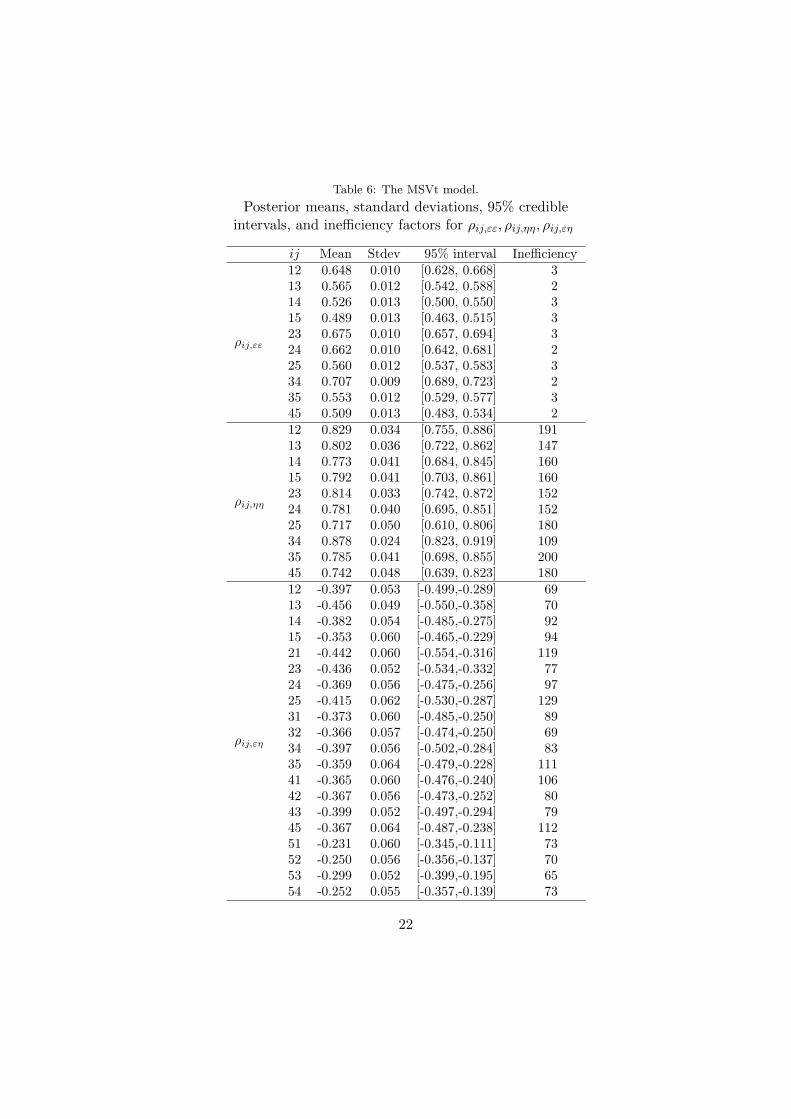
Table 6: The MSVt model.

Posterior means, standard deviations, 95% credibleintervals, and inefficiency factors for ρij,εε, ρij,ηη, ρij,εη

ij Mean Stdev 95% interval Inefficiency

ρij,εε

12 0.648 0.010 [0.628, 0.668] 313 0.565 0.012 [0.542, 0.588] 214 0.526 0.013 [0.500, 0.550] 315 0.489 0.013 [0.463, 0.515] 323 0.675 0.010 [0.657, 0.694] 324 0.662 0.010 [0.642, 0.681] 225 0.560 0.012 [0.537, 0.583] 334 0.707 0.009 [0.689, 0.723] 235 0.553 0.012 [0.529, 0.577] 345 0.509 0.013 [0.483, 0.534] 2

ρij,ηη

12 0.829 0.034 [0.755, 0.886] 19113 0.802 0.036 [0.722, 0.862] 14714 0.773 0.041 [0.684, 0.845] 16015 0.792 0.041 [0.703, 0.861] 16023 0.814 0.033 [0.742, 0.872] 15224 0.781 0.040 [0.695, 0.851] 15225 0.717 0.050 [0.610, 0.806] 18034 0.878 0.024 [0.823, 0.919] 10935 0.785 0.041 [0.698, 0.855] 20045 0.742 0.048 [0.639, 0.823] 180

ρij,εη

12 -0.397 0.053 [-0.499,-0.289] 6913 -0.456 0.049 [-0.550,-0.358] 7014 -0.382 0.054 [-0.485,-0.275] 9215 -0.353 0.060 [-0.465,-0.229] 9421 -0.442 0.060 [-0.554,-0.316] 11923 -0.436 0.052 [-0.534,-0.332] 7724 -0.369 0.056 [-0.475,-0.256] 9725 -0.415 0.062 [-0.530,-0.287] 12931 -0.373 0.060 [-0.485,-0.250] 8932 -0.366 0.057 [-0.474,-0.250] 6934 -0.397 0.056 [-0.502,-0.284] 8335 -0.359 0.064 [-0.479,-0.228] 11141 -0.365 0.060 [-0.476,-0.240] 10642 -0.367 0.056 [-0.473,-0.252] 8043 -0.399 0.052 [-0.497,-0.294] 7945 -0.367 0.064 [-0.487,-0.238] 11251 -0.231 0.060 [-0.345,-0.111] 7352 -0.250 0.056 [-0.356,-0.137] 7053 -0.299 0.052 [-0.399,-0.195] 6554 -0.252 0.055 [-0.357,-0.139] 73

22

Tables 6 shows the posterior means, standard deviations, 95% credibleintervals and inefficiency factors for ρij,εε, ρij,ηη, and ρij,εη. Very high corre-lations are found among εits (with ρij,εεs ranging from 0.489 to 0.707), andamong ηits (with ρij,ηηs ranging from 0.717 to 0.878), which may cause thelow absolute values of ρi,ϵηs as mentioned above.

The posterior means of ρij,εη are all negative and vary from −0.456 to−0.231, and none of the 95% credible intervals for ρij,εη include zero. This isstrong evidence for the existence of cross asset leverage effects. Furthermore,we note that the cross leverage effects between series i and j are foundto be asymmetric, i.e., ρij,εη = ρji,εη for i = j. For example, in Table6, ρi5,εηs vary from −0.415 to −0.353, while ρ5j,εηs vary from −0.299 to−0.231. This means the cross leverage effects from Series 1, 2, 3, and 4 onthe volatility of Series 5 (i.e., ‘Utilities’) are relatively stronger than vice-versa. The volatility of the ‘Utilities’ series is more influenced by decreasesin returns of four other series, while those of the other series are less subjectto change in the returns of ‘Utilities’ series. This would suggest that marketparticipants do not react so sharply when a decrease in the return is limitedto ‘Utilities’ series, but they do react in a more sensitive way if decreasesoccur in other series.

4.4. Model comparison

Finally, we conduct a comparison of the MSV and MSVt models usingthe deviance information criterion (DIC) (Spiegelhalter et al. (2002)). TheDIC is defined by

DIC = Eθ|y[D(θ)] + pD,

where

pD = Eθ|y[D(θ)]−D(Eθ|y[θ]), D(θ) = −2 log f(Yn|θ).

To compute Eθ|y[D(θ)], we use a sample analogue, 1M

∑Mm=1D(θ(m)), where

we set M = 100, and θ(m)s are resampled from the posterior distribution.The numerical standard error of the estimate is obtained by repeatedly es-timating Eθ|y[D(θ)] ten times. Regarding D(Eθ|y[θ]), which equals to D(θ)evaluated at the posterior mean, we implement an auxiliary particle filter tocompute the likelihood ordinate log f(Yn|θ) as discussed in Section 2.3 andset the number of particles, I = 10, 000. We repeat this ten times to obtainthe numerical standard error.

23

Table 7 shows the sample means of DIC, the standard errors, and thesmallest and the largest values among one hundred DIC values computedfor two competing models. The DIC of the MSVt model much smaller thanthat of the MSV model, which indicates that the MSVt models outperformsthe MSV model. This result also constitutes the evidence that the S&P500sector index returns are heavy-tailed.

Table 7: Estimates, standard errors and the smallest and the largest values of DIC

Model DIC (s.e.) DICmax DICmin

MSV 48741.6 (1.4) 48749.9 48728.4MSVt 48650.3 (2.6) 48664.8 48634.2

5. Conclusion

This paper proposes an efficient MCMC algorithm using a multi-movesampler for latent volatility vectors for MSV models with cross leverageand heavy-tailed errors. To sample a block of state vectors, we construct aproposal density function for the MH algorithm based on the approximatenormal distribution using Taylor expansion of the logarithm of the targetlikelihood. We then exploit the sampling algorithms, which are developedfor the linear and Gaussian state space models. We show that our proposedmethods are easy to implement and that they are highly efficient. Extend-ing to the model with respect to multivariate t-distributed errors is alsodiscussed. Illustrative examples and empirical analyses are presented basedon five sectors of S&P500 indices.

Acknowledgment

The authors are grateful to Erricos Kontoghiorghes, Guest editor, twoanonymous referees, Siddhartha Chib, Mike K P So, and Boris Choy forhelpful comments and discussions. This work is supported by the ResearchFellowship (DC1) from the Japan Society for the Promotion of Science andthe Grants-in-Aid for Scientific Research (A) 21243018 from the JapaneseMinistry of Education, Science, Sports, Culture, and Technology. The com-putational results are generated using Ox (Doornik (2006)).

24

Appendix

A. Multi-move sampler for the MSV model

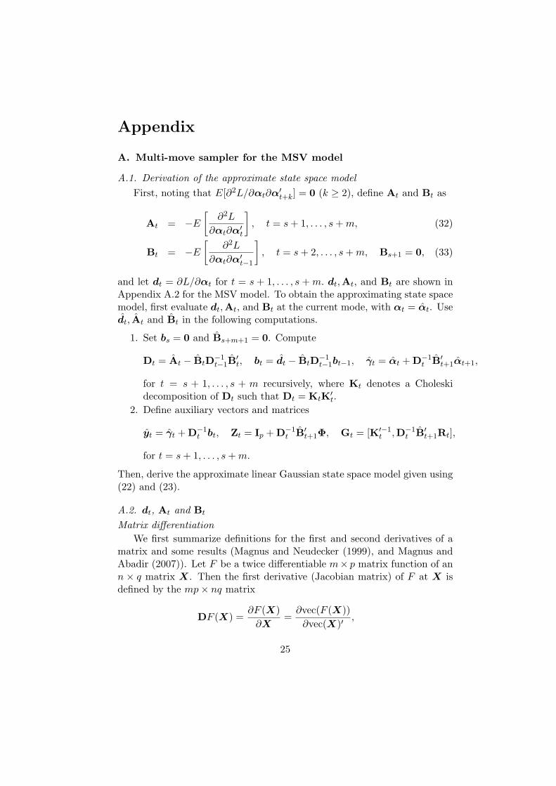
A.1. Derivation of the approximate state space model

First, noting that E[∂2L/∂αt∂α′t+k] = 0 (k ≥ 2), define At and Bt as

At = −E

[∂2L

∂αt∂α′t

], t = s+ 1, . . . , s+m, (32)

Bt = −E

[∂2L

∂αt∂α′t−1

], t = s+ 2, . . . , s+m, Bs+1 = 0, (33)

and let dt = ∂L/∂αt for t = s + 1, . . . , s +m. dt,At, and Bt are shown inAppendix A.2 for the MSV model. To obtain the approximating state spacemodel, first evaluate dt,At, and Bt at the current mode, with αt = αt. Usedt, At and Bt in the following computations.

1. Set bs = 0 and Bs+m+1 = 0. Compute

Dt = At − BtD−1t−1B

′t, bt = dt − BtD

−1t−1bt−1, γt = αt +D−1

t B′t+1αt+1,

for t = s + 1, . . . , s + m recursively, where Kt denotes a Choleskidecomposition of Dt such that Dt = KtK

′t.

2. Define auxiliary vectors and matrices

yt = γt +D−1t bt, Zt = Ip +D−1

t B′t+1Φ, Gt = [K′−1

t ,D−1t B′

t+1Rt],

for t = s+ 1, . . . , s+m.

Then, derive the approximate linear Gaussian state space model given using(22) and (23).

A.2. dt, At and Bt

Matrix differentiation

We first summarize definitions for the first and second derivatives of amatrix and some results (Magnus and Neudecker (1999), and Magnus andAbadir (2007)). Let F be a twice differentiable m× p matrix function of ann × q matrix X. Then the first derivative (Jacobian matrix) of F at X isdefined by the mp× nq matrix

DF (X) =∂F (X)

∂X=

∂vec(F (X))

∂vec(X)′,

25

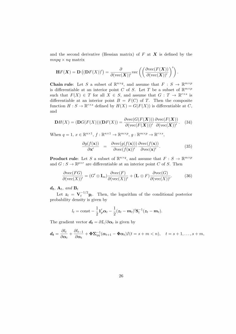
and the second derivative (Hessian matrix) of F at X is defined by themnpq × nq matrix

HF (X) = D((DF (X))′

)=

∂

∂(vec(X))′vec

((∂vec(F (X))

∂(vec(X))′

)′).

Chain rule: Let S a subset of Rn×q, and assume that F : S → Rm×p

is differentiable at an interior point C of S. Let T be a subset of Rm×p

such that F (X) ∈ T for all X ∈ S, and assume that G : T → Rr×s isdifferentiable at an interior point B = F (C) of T . Then the compositefunction H : S → Rr×s defined by H(X) = G(F (X)) is differentiable at C,and

DH(X) = (DG(F (X)))(DF (X)) =∂vec(G(F (X)))

∂(vec(F (X)))′∂vec(F (X))

∂(vec(X))′. (34)

When q = 1, x ∈ Rn×1, f : Rn×1 → Rm×p, g : Rm×p → Rr×s,

∂g(f(x))

∂x′ =∂vec(g(f(x)))

∂vec(f(x))′∂vec(f(x))

∂vec(x)′. (35)

Product rule: Let S a subset of Rn×q, and assume that F : S → Rm×p

and G : S → Rp×r are differentiable at an interior point C of S. Then

∂vec(FG)

∂(vec(X))′= (G′ ⊗ Im)

∂vec(F )

∂(vec(X))′+ (Ir ⊗ F )

∂vec(G)

∂(vec(X))′. (36)

dt, At, and Bt

Let zt = V−1/2t yt. Then, the logarithm of the conditional posterior

probability density is given by

lt = const− 1

21′pαt −

1

2(zt −mt)

′S−1t (zt −mt).

The gradient vector dt = ∂L/∂αt is given by

dt =∂lt∂αt

+∂lt−1

∂αt+ΦΣ−1

ηη (αt+1 −Φαt)I(t = s+m < n), t = s+ 1, . . . , s+m,

26

where

∂lt∂α′

t

= −1

21′p − (zt −mt)

′S−1t

∂(zt −mt)

∂α′t

= −1

21′p +

1

2(zt −mt)

′S−1t

{diag(zt)− 2ΣεηΣ

−1ηη ΦI(t < n)

},(37)

∂lt−1

∂α′t

= (zt−1 −mt−1)′S−1

t−1

∂mt−1

∂α′t

= (zt−1 −mt−1)′S−1

t−1ΣεηΣ−1ηη I(t > 1), (38)

using the chain rule (35). Thus

dt = −1

21p +

1

2

{diag(zt)− 2ΦΣ−1

ηη ΣηεI(t < n)}S−1t (zt −mt)

+Σ−1ηη ΣηεS

−1t−1(zt−1 −mt−1)I(t > 1)

+ΦΣ−1ηη (αt+1 −Φαt)I(t = s+m < n),

for t = s+ 1, . . . , s+m.To compute At and Bt using the product rule (36), we first obtain the

Hessian matrix

∂2L

∂αt∂α′t

=∂2lt

∂αt∂α′t

+∂2lt−1

∂αt∂α′t

−ΦΣ−1ηη ΦI(t = s+m < n),

for t = s+ 1, . . . , s+m where

∂2lt∂αt∂α′

t

=

1

2

{(zt −mt)

′S−1t ⊗ Ip

} ∂vec(diag(zt))

∂α′t

−1

4

(diag(zt)− 2ΦΣ−1

ηη ΣηεI(t < n))S−1t

(diag(zt)− 2ΣεηΣ

−1ηη ΦI(t < n)

),

(39)

and

∂2lt−1

∂αt∂α′t

= −Σ−1ηη ΣηεS

−1t−1ΣεηΣ

−1ηη I(t > 1). (40)

27

Noting that

∂vec(diag(zt))

∂α′t

= −1

2

z1te1e′1

...zptepe

′p

, E [zjt(zt −mt)] = Stej , (41)

where ej is a p×1 unit vector with j-th component equal to 1, the expectedvalue of the first term in (39) is

E

[{(zt −mt)

′S−1t ⊗ Ip

} ∂vec(diag(zt))

∂α′t

]= −1

2

p∑j=1

(e′jS−1t )(Stej)eje

′j

= −1

2Ip, (42)

Further, using diag(zt)S−1t diag(zt) = S−1

t ⊙ (ztz′t), the expected value of

the second term in (39) is

E[(diag(zt)− 2ΦΣ−1

ηη ΣηεI(t < n))S−1t

(diag(zt)− 2ΣεηΣ

−1ηη ΦI(t < n)

)]= S−1

t ⊙ (St +mtm′t) + 4ΦΣ−1

ηη ΣηεS−1t ΣεηΣ

−1ηη ΦI(t < n) (43)

−2(ΦΣ−1

ηη ΣηεS−1t diag(mt) + diag(mt)S

−1t ΣεηΣ

−1ηη Φ

)I(t < n)

Thus, we obtain

At =1

4

{Ip + S−1

t ⊙ (St +mtm′t)}+ΦΣ−1

ηη ΣηεS−1t ΣεηΣ

−1ηη ΦI(t < n)

−1

2

(ΦΣ−1

ηη ΣηεS−1t diag(mt) + diag(mt)S

−1t ΣεηΣ

−1ηη Φ

)I(t < n)

+Σ−1ηη ΣηεS

−1t−1ΣεηΣ

−1ηη I(t > 1) +ΦΣ−1

ηη ΦI(t = s+m < n), (44)

for t = s+ 1, . . . , s+m. Similarly, it is straightforward to show that

Bt = −E

[∂2lt−1

∂αt∂α′t−1

]=

1

2Σ−1

ηη ΣηεS−1t−1

{diag(mt−1)− 2ΣεηΣ

−1ηη Φ

}, (45)

for t = s+ 2, . . . , s+m.

References

Asai, M., McAleer, M., 2006. Asymmetric multivariate stochastic volatility. Econo-metric Reviews 25, 453–473.

28

Asai, M., McAleer, M., Yu, J., 2006. Multivariate stochastic volatility: A review.Econometric Reviews 25, 145–175.

Broto, C., Ruiz, E., 2004. Estimation methods for stochastic volatility models: asurvey. Journal of Economic Survey 18, 613–649.

Chan, D., Kohn, R., Kirby, C., 2006. Multivariate stochastic volatility models withcorrelated errors. Econometric Reviews 25, 245–274.

Chib, S., 2001. Markov chain Monte Carlo methods: computation and inference. In:Heckman, J. J., Leamer, E. (Eds.), Handbook of Econometrics. Vol. 5. North-Holland, Amsterdam, pp. 3569–3649.

Chib, S., Nardari, F., Shephard, N., 2006. Analysis of high dimensional multivariatestochastic volatility models. Journal of Econometrics 134, 341–371.

Chib, S., Omori, Y., Asai, M., 2009. Multivariate stochastic volatility. In: Andersen,T. G., Davis, R. A., Kreiss, J. P., Mikosch, T. (Eds.), Handbook of FinancialTime Series. Springer-Verlag, New York, pp. 365–400.

de Jong, P., Shephard, N., 1995. The simulation smoother for time series models.Biometrika 82, 339–350.

Doornik, J., 2006. Ox: Object Oriented Matrix Programming. Timberlake Consul-tants Press, London.

Doucet, A., de Freitas, N., Gordon, N. J. (Eds.), 2001. Sequential Monte CarloMethods in Practice. Springer-Verlag, New York.

Durbin, J., Koopman, S. J., 2002. A simple and efficient simulation smoother forstate space time series analysis. Biometrika 89, 603–616.

Jacquier, E., Polson, N. G., Rossi, P. E., 1999. Stochastic volatility: Univariate andmultivariate extensions, cIRANO Working paper 99s–26, Montreal.

Koopman, S. J., 1993. Disturbance smoother for state space models. Biometrika80, 117–126.

Liesenfeld, R., Richard, J.-F., 2003. Univariate and multivariate stochastic volatilitymodels: Estimation and diagnostics. Journal of Empirical Finance 10, 505–531.

Lopes, H. F., Carvalho, C. M., 2007. Factor stochastic volatility with time vary-ing loadings and Markov switching regimes. Journal of Statistical Planning andInference 137, 3082–3091.

Magnus, J. R., Abadir, K. M., 2007. On some definitions in matrix algebra, discus-sion paper, CIRJE-F-476, Faculty of Economics, University of Tokyo.

29

Magnus, J. R., Neudecker, H., 1999. Matrix differential culculus with applicationsin statistics and econometrics, revised edition. John Wiley, Chichester.

Nakajima, J., Omori, Y., 2009. Leverage, heavy-tails and correlated jumps instochastic volatility models. Computational Statistics and Data Analysis 53-6,2335–2353.

Omori, Y., Chib, S., Shephard, N., Nakajima, J., 2007. Stochastic volatility withleverage: fast likelihood inference. Journal of Econometrics 140, 425–449.

Omori, Y., Watanabe, T., 2008. Block sampler and posterior mode estimationfor asymmetric stochastic volatility models. Computational Statistics and DataAnalysis 52-6, 2892–2910.

Pitt, M. K., Shephard, N., 1999. Time varying covariances: a factor stochasticvolatility approach. In: Bernardo, J. M., Berger, J. O., Dawid, A. P., Smith, A.F. M. (Eds.), Bayesian Statistics. Vol. 6. Oxford University Press, Oxford, pp.547–570.

Shephard, N., Pitt, M. K., 1997. Likelihood analysis of non-Gaussian measurementtime series. Biometrika 84, 653–667.

So, M. K. P., Choi, C. Y., 2009. A threshold factor multivariate stochastic volatilitymodel. Journal of Forecasting 28-8, 712–735.

Spiegelhalter, D. J., Best, N. G., Carlin, B. P., van der Linde, A., 2002. Bayesianmeasures of model complexity and fit (with discussion). Journal of the RoyalStatistical Society, Series B 64, 583–639.

Takahashi, M., Omori, Y., Watanabe, T., 2009. Estimating stochastic volatilitymodels using daily returns and realized volatility simultaneously. ComputationalStatistics and Data Analysis 53-6, 2404–2426.

30