Astron. Astrophys. 329, 1059–1074 (1998) ASTRONOMYAND

ASTROPHYSICS

Circumstellar molecular radio line intensity ratios

H. Olofsson1, M. Lindqvist2, L–A. Nyman2,3, and A. Winnberg2

1 Stockholm Observatory, S-133 36 Saltsjobaden, Sweden2 Onsala Space Observatory, S-439 92 Onsala, Sweden3 ESO/La Silla, Casilla 19001, Santiago 19, Chile

Received 13 June 1997 / Accepted 3 September 1997

Abstract. We have observed a sample of 61 AGB–stars (39 M–stars and 22 C–stars) in circumstellar CO, CS, HCN, SiO, SiS,and SO radio line emission. The main results presented are basedon the use of line intensity ratios, a well defined observationalquantity that can be used to infer important conclusions as wellas to provide constraints on models. Taken together the data arefully consistent with the facts that for this sample the circum-stellar envelopes have the same basic chemistry (i.e., C/O<1 or>1) as the central stars, and that the mass loss rates have notchanged drastically over periods between 102–103 years. TheHCN(J = 1→0)/SiO(J = 2→1) intensity ratio discriminatesunambiguously between “normal” circumstellar envelopes withC/O<1 (O–CSEs) and>1 (C–CSEs), while the CS(J = 2→1),HCN(J = 1→0), SiO(J = 2→1), and SiS(J = 5→4) intensityratios with respect to CO(J = 1→0) are not perfect for thispurpose, and neither is the SiS(J = 5→4)/SiO(J = 2→1) in-tensity ratio. The data further shows that SO and the C-bearingmolecule HCN are ubiquitously present in O–CSEs, and thattheir line intensities in O–CSEs are qualitatively consistent withthe fact that the molecules are formed in a photo–induced cir-cumstellar chemistry in a quantity that depends on the mass lossrate. Hence, both species can in principle be used to estimatethe mass loss rate, and the tight relation between the SO(JK =32→21) and CO(J = 1→0) intensities in O–CSEs shows thatSO line emission may even be a good mass loss rate estimator.On the contrary, the SiO(J = 2→1) luminosity appears to be es-sentially independent of the mass loss rate in O–CSEs, possiblydue to a larger influence from molecular adhesion onto grains.These results explain why the HCN(J = 1→0)/SiO(J = 2→1)intensity ratio increases with the mass loss rate in O–CSEs, andthere is no need to invoke e.g. a spread in C/O–ratios for theM–stars to explain the large range of this ratio.

Maser emission is very likely present in the HCN(J = 1→0)line in C–CSEs, and it seems to be sensitively dependent on themass loss rate, i.e., it appears only for M <∼ 5×10−7 M� yr−1.Based on time monitoring of this emission towards the C–starsW Ori and X TrA, we suggest that the strongest maser featuresare due to radial amplification in the F = 2→1 transition. The

Send offprint requests to: H. Olofsson (hans@astro.su.se)

predominance of redshifted maser emission could be caused byan additional amplification in the F = 1→1 transition. We findno evidence for a similar maser in O–CSEs.

Key words: masers – stars: carbon – circumstellar matter –stars: mass–loss – stars: AGB, post–AGB – radio lines: stars

1. Introduction

An impressive number of different molecular species (≈60) andtheir isotopic variants have been found in the circumstellar en-velopes (CSEs) that are formed around asymptotic giant branch(AGB) stars through their intense mass loss (Olofsson 1997a).Some of these molecules are of photospheric origin, but the ma-jority are produced through various chemical processes in theenvelope itself. This chemistry depends primarily on the chemi-cal composition of the gas (i.e., C/O<1 or>1), but the physicalconditions also change as the central star evolves along the AGBand beyond. The relative simplicity of the envelopes, i.e., theirgeometry and kinematics, and the large variety in their physicaland chemical characteristics, make them excellent laboratoriesfor studying molecular formation processes in an astrophysi-cal context. However, the circumstellar molecules are also im-portant probes in the study of late stellar evolution (Olofsson1997a,c).

The photospheric species are produced in an equilibriumchemistry in the atmosphere of the central star (see e.g., Tsuji1964, 1973; Lafont et al. 1982; Glassgold & Huggins 1983;Cherchneff & Barker 1992). The main problem is that the molec-ular abundances normally vary with the height in the atmo-sphere, and it is not clear which abundances to adopt for theescaping gas. Furthermore, there may be significant departuresfrom equilibrium due to e.g. shocks propagating through the at-mosphere and dust formation. These parent molecules are even-tually photodissociated, which results in the direct formation ofthe photodissociation products, as well as the indirect formationof other species by providing the ingredients of a circumstellarchemistry. The latter has been studied theoretically in a numberof papers, both for the chemical compositions of O– (see e.g.,

1060 H. Olofsson et al.: Circumstellar molecular radio line intensity ratios

Scalo & Slavsky 1980; Huggins & Glassgold 1982; Nejad &Millar 1988; Nercessian et al. 1989; Millar & Olofsson 1993;Charnley et al. 1995; Willacy & Millar 1997) and C–CSEs (seee.g., Lafont et al. 1982; Nejad & Millar 1987; Glassgold et al.1992; Cherchneff & Glassgold 1993; Millar & Herbst 1994).

Circumstellar molecules have also been extensively ob-served, both in the form of surveys in a single molecular speciesand in the form of searches for various molecular species in alimited number of carefully selected sources (Olofsson 1997b).We will here concentrate on studies aimed at estimating molec-ular abundances. Olofsson et al. (1993b) performed a survey ofHCN, CN, and CS in a sample of bright carbon stars (57 objects,39 detections of HCN). They found that the circumstellar HCNabundance have a reasonable dependence on the correspond-ing photospheric abundance, and that the circumstellar CN is aphotodissociation product, but they also concluded that there islikely to be considerable systematic errors in their abundance es-timates caused by imperfections of the model for the circumstel-lar emission. The latter was further emphasized by Izumiura etal. (1995) who pointed out that the brightnesses of the HCN(J =1→0) line in C–CSEs are not consistent with the expectedsizes of the emitting regions. Bujarrabal et al. (1994a) estimateda number of molecular abundances (e.g., HCN, CS, SiO, andSiS) in a sample of 16 C–CSEs, and Bachiller et al. (1997) esti-mated the CN abundances in 26 C–CSEs. Nyman et al. (1993)compared more than 10 circumstellar molecular abundances forthe high mass loss C–stars IRC+10216 and IRAS15194–5115.HCN has also been extensively observed in O–CSEs (≈20 de-tections; Lindqvist et al. 1988, 1992; Nercessian et al. 1989;Bujarrabal et al. 1994a), and to a lesser extent has CN (2 AGB–stars and 3 supergiants; Olofsson et al. 1991; Bachiller et al.1997). Recently, Charnley & Latter (1997) searched a num-ber of O–CSEs for C2H and CH3OH without success. Speciesconsiderably more characteristic for, and probably unique to,O–CSEs are SO and SO2, and they have also been detected in≈20 sources each (see e.g., Sahai & Wannier 1992; Omont etal. 1993). Bieging & Latter (1994) extended this type of workto CSEs around S–stars, where they concentrated on HCN andSiO. However, the conclusion to be drawn from these studiesis that absolute abundances are fairly uncertain, by at least anorder of magnitude, and can at best be used for studying trends,or differences in the chemistry between O– and C–CSEs. Moresophisticated models are required in order to make significantprogress here, but some of the crucial observational data arestill largely missing, e.g., direct measurements of the brightnessdistributions.

Bujarrabal et al. (1994a,b) showed that even simple molec-ular line intensity ratios, if properly chosen, may be used toinfer important conclusions. For instance, it is possible to dis-tinguish between “normal” O– and C–CSEs (Bujarrabal et al.1994b; by a “normal” CSE we here mean one that has beenproduced by a relatively constant mass loss of constant chemi-cal composition over a relatively long time scale, <∼103 years),and Olofsson et al. (1993b) and Bujarrabal & Cernicharo (1994)used them to identify anomalous CSEs. The use of line intensityratios has the advantage of requiring no assumptions about a cir-

Table 1. Overview of the observations

Freq. O–CSEs C–CSEs[GHz] detected negative detected negative

CO(J = 1→0) 115.3 37 - a 22 -HCN(J = 1→0) 88.6 19 20 22 -SiO(J = 2→1) 86.8 29 - 12 10SO(JK = 22→11) 86.1 - 4 - -SO(JK = 32→21) 99.3 16 5 - -SiS(J = 5→4) 90.8 3 3 7 6CS(J = 2→1) 98.0 2 5 15 7

a Two M–stars were not detected in CO because of problems withinterfering interstellar CO emission

cumstellar model, but it also limits the type of conclusions thatcan be drawn. In this paper we proceed along this line, therebyconsiderably strengthening some of the conclusions drawn byBujarrabal et al. (1994a,b), as well as obtaining a number ofnew results that will serve as constraints on chemical and cir-cumstellar models.

2. Sample

We report results on circumstellar CO, CS, HCN, SiO, SiS, andSO radio line observations of 61 AGB–stars, 39 M–stars (≈70%Miras and ≈30% Semiregulars) and 22 C–stars (≈40% Mirasand ≈60% Semiregulars).

The M–stars were chosen among stars spectroscopicallyclassified as M–stars (Kholopov et al. 1985), and/or have emis-sion in at least one of the masing lines of OH, H2O, or SiO(Engels & Heske 1989; Benson et al. 1990), and/or have anLRS-class 2n (Olnon & Raymond 1986). This makes it verylikely that the associated CSEs also have elemental composi-tions where C/O<1. The majority of the C–stars are well knowncarbon stars, e.g, a fair fraction (≈55%) of them belong to thesample studied by Lambert et al. (1986), and except for S Cepand RV Cyg they have an LRS–class 4n. The associated CSEsvery likely have elemental compositions where C/O>1. Fromnow on we will refer to CSEs around M– and C–stars as O– andC–CSEs, respectively, assuming that the C/O-ratio of the cen-tral star and the CSE agree with each other. As will be shown,there is nothing in our data that contradicts this assumption. Thevariability type was taken from Kholopov et al. (1985). We haveused the best coordinates available at the time of the observa-tion (see e.g., Loup et al. 1993). Only in a few cases have weretreated to the IRAS coordinates.

The distances, D, for the M–stars are obtained by integrat-ing visual, near-infrared, and IRAS data assuming a luminosityof 5000 L� for the Semiregulars (Kerschbaum & Hron 1996),using the period–luminosity relation obtained by Whitelock etal. (1994) for the Miras, and assuming a luminosity of 104 L�for those stars where the variability class is not known. For theoptically bright C–stars we adopt the method used in Olofs-son et al. (1993a), i.e., we assume an absolute K–magnitudeof -8.1, while for the more extreme C–stars (V384 Per, 07454–

H. Olofsson et al.: Circumstellar molecular radio line intensity ratios 1061

7112, CW Leo, RW LMi, 15082–4808, 15194–5115) we adoptvalues from the literature (e.g., Sopka et al. 1989; Loup et al.1993).

3. Observations

An overview of the observations are given in Table 1 and theobservational results are given in Table 2. All data have beenobtained with the Onsala 20m telescope (OSO), Sweden, andthe Swedish-ESO Submillimetre Telescope (SEST) on La Silla,Chile, by us (this paper; Lindqvist et al. 1988, 1992) or by others(Nyman et al. 1992; Olofsson et al. 1993a,b; Kerschbaum et al.1996; Larsen et al. 1997; Nyman & Olofsson 1997) during theperiod 1987–1997. For each star the same telescope has beenused for all observed transitions. This data base is larger thanthe one used in a similar study by Bujarrabal et al. (1994a): 30AGB–stars, 14 M–stars (e.g., 9 detections of HCN, 7 detectionsof SO), 16 C–stars (e.g., 10 detections of SiO).

The line intensities, integrated over velocity, are given in themain beam brightness scale, i.e., the antenna temperature hasbeen corrected for the atmospheric attenuation (using the chop-per wheel method) and divided by the main beam efficiency.The latter is≈0.6–0.5 (≈0.4–0.3 for data obtained before March1993) in the frequency range 86–115 GHz for OSO, and≈0.75in the same frequency range for SEST. The upper limits are cal-culated using the peak–to–peak value, Tpp, of a spectrum witha velocity resolution reduced to twice the expansion velocity ofthe CSE, i.e., Iupper = 2Tppve. This should provide a conserva-tive upper limit. The gas expansion velocities, ve, are obtainedas half the full width at zero power of the CO(J = 1→0) lineprofiles. The telescope used is indicated by O for OSO and Sfor SEST. The beam widths lie in the ranges 33′′–42′′ for OSOand 45′′–60′′ for SEST, respectively.

New detections not yet reported in the literature areCS: V384 Per, S Cep (from Larsen et al. 1997) and 07454–7112, 15082–4808 (from Nyman & Olofsson 1997); HCN:R Leo, CIT4, IRC+50137; SiO: R For, V384 Per, R Lep, R Vol,RV Aqr, and 07454–7112, 15082–4808 (from Nyman & Olofs-son 1997); SO: R Dor, GX Mon, W Hya, RS CrA, R Aql, CIT4,IRC+70066; SiS: WX Psc, and V384 Per, V Cyg (from Larsenet al. 1997), and 07454–7112, 15082–4808 (from Nyman &Olofsson 1997). Spectra of the new detections are presented inFig. 1 [except those that will be published in Larsen et al. (1997)and Nyman & Olofsson (1997)].

4. Molecular line intensity ratios

The line intensity ratios to be discussed are HCN (J = 1→0) /CO (J = 1→0), SiO (J = 2→1) / CO(J = 1→0), HCN (J =1→0) / SiO (J = 2→1), and SO (JK = 32→21) / CO(J =1→0). Line intensity ratios involving CS and SiS are not dis-cussed at any lengths due to the small number of detections ofthese species in O–CSEs. The results of the line intensity ratiosare summarized in Table 3. We find no evidence that the molec-ular line intensity ratios are dependent on the beam size (e.g.,due to partial resolution of the brightness distributions), and

therefore OSO and SEST data are not separated in the analysis.This also means that the results should apply to any telescopeas long as the effect of beam filling can be ignored.

We have not estimated the formal error of each individualline intensity ratio for the following reason. We found the inten-sity of the calibration sources to be repeatable at the±10% levelat both OSO and SEST. If we include pointing uncertainties theintensity scale is estimated to have an uncertainty of ±15%.The absolute calibration of the intensity scale is not of interesthere since we are only using line intensity ratios obtained usingdata from the same telescope. Some of the lines are quite weak(in practice those for which I < 1 K km s−1), and for those weestimate that the line intensity ratio (which always involve oneline that is reasonably strong) is uncertain by at most ±50%.Thus, we expect the uncertainties to lie in the range ±20% to±50%. This will have no effect on the conclusions drawn in thispaper.

We will first introduce a simple mass loss rate measure,adequate for discussing the dependences of various molecularline intensity ratios on the mass loss rate of the central object.

4.1. A mass loss rate measure

Amongst other things, we are interested in looking at the depen-dences of the line intensity ratios on the mass loss rate. To obtainthe absolute mass loss rate of a star from e.g. its CO line emis-sion requires relatively detailed modelling (see e.g., Sahai 1990;Kastner 1992; Kwan & Webster 1993; Groenewegen 1994; Just-tanont et al. 1994). However, we are only interested in trendsand not in the absolute mass loss rates of the individual stars. Wehave therefore decided to compare our results with the simplemass loss rate measure ICOveD

2 [it is reasonable to assume thatthis expression contains all the observational quantities, as wellas the main functional dependence of the mass loss rate on them,that are required to estimate the mass loss rate, see e.g., Kast-ner 1992)], where ICO is the velocity–integrated intensity of theCO(J = 1→0) line in K km s−1, ve is given in km s−1, and Dis given in kpc (we will in the following not repeat the somewhatawkward unit of the mass loss rate measure, K km2 s−2 kpc2).In doing this we have scaled the SEST CO intensities to theOnsala scale by simply assuming that the intensity increases inproportion to the telescope area. In Fig. 2 we compare ICOveD

2

with mass loss rate estimates obtained from model work (Sopkaet al. 1989; Kahane & Jura 1994; Justtanont et al. 1994), and, forthe low–M C–CSEs, from Loup et al. (1993). There is clearlya good correlation although the relation is weaker than a linearone, so that a change in the mass loss rate measure by threeorders of magnitude corresponds to a change in the mass lossrate by about two orders of magnitude. There is no significantdifference between O– and C–CSEs in this respect. A fit to thedata (irrespective of the chemistry) results in

M = 2.0× 10−7 (ICOveD2)0.59 M� yr−1, (1)

with a correlation coefficient of 0.92.In Fig. 3 we plot our stars in a two–colour diagram based

on the IRAS–fluxes. The area of the symbols are proportional

1062 H. Olofsson et al.: Circumstellar molecular radio line intensity ratios

Table 2. Observational results

Source IRAS Var. D Tel.a ve Imb [ K km s−1][pc] [ km s−1] CO(1-0) b CS(2-1) HCN(1-0) SiO(2-1) SiS(5-4) SO(32-21) SO(22-11)

M–stars:IRC+40004 00042 + 4248 M 410 O 19.3 24.8 <0.6 1.1T Cas 00205 + 5530 M 360 O 10.6 2.0 <0.9WX Psc 01037 + 1219 M 600 O 19.3 52.0 <0.8 3.7 9.7 1.4 5.8 <0.4BD+44398 01556 + 4511 250 O 9.4 3.9 <1.1CIT4 02316 + 6455 290 O 19: 15: 0.7: 1.7 1.4:R Hor 02522 − 5005 M 280 S 5.5 2.5 <0.4IK Tau 03507 + 1115 M 250 O 18.5 58.2 0.5 3.5 15.8 0.3 3.6 <0.4R Dor 04361 − 6210 SRb 70 S 6.2 5.0 0.6 13.5 0.5TX Cam 04566 + 5606 M 380 O 21.5 21: 1.0 4.8 13.0 0.6 2.1 <0.6IRC+50137 05073 + 5248 M 410 O 18.0 19.7 0.9 1.9 1.2IRC+60154 05151 + 6312 330 O 18.8 5.3 <0.6 0.8U Aur 05388 + 3200 M 610 O IS <0.3 0.9IRC+70066 05411 + 6957 470 O 18.5 20.0 1.3 3.3 <0.3 0.9V Cam 05559 + 7430 M 650 O 15.1 3.7 <0.6 1.0IRC+60169 06300 + 6058 490 O 14.4 16.4 <0.6 1.2 4.3 1.2GX Mon 06500 + 0829 M 540 O 18.7 48.6 <1.0 2.3 9.2 2.9RS Cnc 09076 + 3110 SRc: 100 O 7.0 7.3 <0.7IRC–20197 09429 − 2148 M: 340 S 11.5 1.4 <0.3R Leo 09448 + 1139 M 130 O 7.5 2.4 0.4 4.5 <0.4R Crt 10580 − 1803 SRb 180 S 10.3 5.0 0.5 5.7RT Vir 13001 + 0527 SRb 190 O 9.2 5.1 0.3 4.0 <0.4SW Vir 13114 − 0232 SRb 140 O 8.1 10.2 <0.8 3.5 <0.5R Hya 13269 − 2301 M 150 S 4.0 0.6 <0.4 4.2W Hya 13462 − 2807 SRa 90 S 7.3 0.8 0.4 7.7 0.2:RX Boo 14219 + 2555 SRb 150 O 9.8 13.7 0.5 9.3 1.0S CrB 15193 + 3132 M 380 O 7.9 2.6 <0.6X Her 16011 + 4722 SRb 160 O 6.2 3.9 <0.4 2.6 <0.5g Her 16269 + 4159 SRb 110 O 9: 1.7: <1.1MW Her 17334 + 1537 M 670 O 14.4 5.9 <0.7IRC+10365 18349 + 1023 M 750 O 16.2 21.4 <0.6 2.0 6.0 <0.3 2.2 <1.3IRC–30398 18560 − 2954 M: 390 S 19.6 10.4 0.4 1.2 <0.2RS CrA 18595 − 3947 M: 210 S 18.7 14.9 1.7 5.2 1.3R Aql 19039 + 0809 M 230 O IS <0.6 5.0 1.1RR Aql 19550 − 0201 M 430 O 7.2 4.2 <0.5 0.9IRC–10529 20077 − 0625 M: 270 O 16.0 28.0 1.0 2.9 3.7T Cep 21088 + 6817 M 220 O 6.9 1.7 <1.1 0.6EP Aqr 21439 − 0226 SRb 140 S 9.8 5.1 <1.0TW Peg 22017 + 2806 SRb 220 O 9.8 2.3 <1.0R Cas 23558 + 5106 M 220 O 14.3 14.4 <0.4 1.3 8.6 <0.4 1.7

C–stars:R For 02270 − 2619 M 670 S 16.3 4.8 0.6 2.0 0.4V384 Per 03229 + 4721 M 650 O 14.2 25.5 6.9 8.0 1.2 0.4U Cam 03374 + 6229 SRb 500 O 24.7 5.8 1.6 3.9 <0.4 <0.3ST Cam 04459 + 6804 SRb 510 O 8.6 2.0 <0.5 2.3 <0.5R Lep 04573 − 1452 M 430 S 17.0 6.2 <0.3 2.3 0.5W Ori 05028 + 0106 SRb 360 O 11.1 2.7 <0.8 4.6 <0.7Y Tau 05426 + 2040 SRb 500 O 15.2 7.0 <0.4 3.5 <1.5UU Aur 06331 + 3829 SRb 300 O 10.9 7.9 <0.5 5.5 <0.5R Vol 07065 − 7256 M 820 S 18.5 4.9 1.3 1.9 0.8: <0.307454–7112 07454 − 7112 750 S 13.6 24.1 2.3 4.1 0.6 0.8CW Leo 09452 + 1330 M 150 O 14.2 310.7 130.0 227.0 29.9 40.6RW LMi 10131 + 3049 SRa 390 O 15.8 75.8 19.2 28.4 3.8 1.3Y CVn 12427 + 4542 SRb 290 O 8.4 4.5 0.7 9.7 <0.4 <0.3RY Dra 12544 + 6615 SRb: 470 O 7.3 2.4 0.9 3.4 <0.4 <0.215082–4808 15082 − 4808 670 S 20.4 38.3 8.6 10.7 2.1 1.1X TrA 15094 − 6953 Lb 320 S 7.8 2.5 <0.4 3.1 <0.315194–5115 15194 − 5115 470 S 22.2 49.0 12.1 17.2 5.4 2.4V Aql 19017 − 0545 SRb 390 O 7.6 3.2 0.2 1.3 <0.4V Cyg 20396 + 4757 M 580 O 13.1 34.0 6.3 9.0 1.2 0.3:RV Aqr 21032 − 0024 M 820 S 14.9 8.0 1.3 2.3 0.7 <0.4S Cep 21358 + 7823 M 440 O 22.0 16.3 7.5 11.8 1.7 <0.2RV Cyg 21412 + 3747 SRb 490 O 13.3 4.8 <0.5 2.0 <0.6

a O = OSO 20m telescope, S = 15m SESTb IS = confusion due to interstellar CO emission

H. Olofsson et al.: Circumstellar molecular radio line intensity ratios 1063

Fig. 1. Spectra of the new detections. The intensity scale is given in main beam brightness temperature. The velocity scale of the WX PscSiS(J = 5→4) spectrum is shifted by 94.1 km s−1

Table 3. Line intensity ratios for detected objects

Ratio O–CSEs C–CSEsobjects mean median min max objects mean median min max

HCN(1−0)CO(1−0) 19 0.10 0.07 0.03a 0.49 22 0.68 0.42 0.17 2.2

SiO(2−1)CO(1−0) 27 1.1 0.28 0.04 10.1 12 0.078 0.075 0.03 0.17HCN(1−0)SiO(2−1) 19 0.24 0.28 0.04 0.46 12 5.6 6.2 2.3 7.6b

SO(32−21)c

CO(1−0) 14 0.086 0.09 0.05a 0.13CS(2−1)CO(1−0) 2 0.029 0.01 0.05 15 0.24 0.25 0.06 0.46SiS(5−4)CO(1−0) 3 0.02 0.004 0.029 7 0.041 0.029 0.01 0.13SiS(5−4)SiO(2−1) 3 0.07 0.02 0.14 7 0.65 0.44 0.25a 1.4

a There is one upper limit lower than this.b There are lower limits higher than this.c The tentative detection of SO in W Hya is not included in the analysis.

1064 H. Olofsson et al.: Circumstellar molecular radio line intensity ratios

10-7

10-6

10-5

10-4

10-1 100 101 102 103

O-CSEsC-CSEs

dM/d

t [M

o yr

-1]

ICOveD2 [K km2 s-2 kpc2]

CW LeoWX Psc

RW LMiV Cyg

GX MonIK TauR Lep

R ForV384 Per

R Crt

S CrB

R CasSW VirRT Vir

R Leo X TrAY CVn ST Cam

Fig. 2. A comparison between the mass loss rate measure ICOveD2 and

mass loss rate estimates taken from the literature (see text for details)

to the mass loss rate measure. It is clear that for the M–stars themass loss rate tends to increase with the [25]/[12]-colour as hasbeen shown by many authors (cf. Bedijn 1987; van der Veen &Rugers 1989), and for the C–stars the high–M objects clusterin the area where blackbodies would be found (cf. Olofsson etal. 1993a). There is also a number of high–M M–stars in theregion where C–stars dominate (VII).

4.2. The HCN/CO line intensity ratio

There is a large difference between the I(HCN,J =1→0)/I(CO,J = 1→0)–distributions for the O– (19 objects)and C–CSEs (22 objects), Fig. 4. The former has a median valueof 0.07 and a maximum value of 0.49 (W Hya), while the lat-ter has a median value of 0.42 and a minimum value of 0.17(07454–7112). The majority of the O–CSEs lies in the narrowrange 0.05–0.1. However, there is some overlap in the sense thattwo out of 19 O–CSEs have ratios above the minimum ratio forthe C–CSEs (possibly another two if one takes into account therelative calibration uncertainties). Thus, the IHCN/ICO–ratio isnot a perfect discriminator between O– and C–CSEs. This re-sult is consistent with the findings of Groenewegen et al. (1996).They found five (probable) C–CSEs with line ratios<0.25 (twoof them have a ratio <0.1) using the SEST. Our mean ratiosfor O– and C–CSEs are 0.10 and 0.68, respectively, i.e., in bothcases in excellent agreement with the values obtained by Bu-jarrabal et al. (1994a), 0.11 and 0.76, respectively. The fourS–stars detected in the HCN(J = 1→0) line by Bieging & Lat-ter (1994) have a mean IHCN/ICO–ratio of 0.17, i.e, close to thegeometrical means of our means (0.27) and medians (0.17) forthe O– and C–CSEs.

The reason for the difference in the IHCN/ICO–distributionsis easily explained. CO is believed to be of photospheric ori-gin in both O– and C–CSEs, and its abundance should roughlyequal that of C in the former and O in the latter. i.e., we ex-pect at most a factor of three in difference in the CO abundancebetween the two types of CSEs. Likewise, HCN is believedto be of photospheric origin in C–CSEs, where its abundance

-2.4

-2.0

-1.6

-1.2

-0.8

-0.4

-1.6 -1.2 -0.8 -0.4 0.0 0.4

2.5l

og(F

60/F

25)

2.5log(F 25 /F12 )

VIa VIb

VII IIIa

I II

Fig. 3. A plot of the observed stars in a two-colour diagram based on theIRAS–fluxes [the regions introduced by van der Veen & Habing (1988)are also shown]. The area of the symbols (O–CSEs, circles; C–CSEs,squares) are proportional to the mass loss rate measure ICOveD

2.M–stars not detected in CO due to problems with interfering inter-stellar CO emission are indicated by crosses

is dependent on the C left-over from the CO formation (a fairfraction of the remaining C is contained in other molecules, e.g.,C2H2, and dust particles). On the contrary, HCN is believed tobe of circumstellar origin in an O–CSE, where it is producedthrough reactions starting with CH+NO and N+CH3, where Nand CHx originate from photodissociation of N2 and CH4, re-spectively (Nejad & Millar 1988; Nercessian et al. 1989; Willacy& Millar 1997). Some doubts have been cast upon this schemesince it obviously produces a much higher CN/HCN abundanceratio than is observed (Olofsson et al. 1991; Bachiller et al.1997), and molecules that should be produced simultaneouslywith HCN, e.g., CH3OH and C2H, are not detected (Charnley &Latter 1997). Millar & Olofsson (1993) explained the detectionof H2CO in OH231.8+4.2 (Lindqvist et al. 1992) using a CH4-based chemistry, but this object is probably of a very differentnature than the ones discussed here.

In Fig. 5 we plot the I(HCN,J = 1→0)/I(CO,J = 1→0)–ratios as a function of the mass loss rate measure ICOveD

2.Except for the high value of W Hya (0.49), it appears that thisline ratio is essentially independent of the mass loss rate overmore than two orders of magnitude for the O–CSEs, the ra-tio is 0.09±0.05 (1σ) for ICOveD

2 > 0.1 (which correspondsto roughly 10−7 M� yr−1). This behaviour very likely has itsroots in the M -dependences of the number of the CO and HCNmolecules and the size of the HCN and CO line–emitting re-gions. The models predict that the radius of the peak abundance,Rp, in the HCN–shell of an O–CSE should increase roughly asM 0.7 [ignoring the dependence on ve, but M substituted with(M/ve) should give roughly the correct dependence; Nerces-sian et al. 1989]. It appears that the relative width of the shell,∆R/Rp, decreases with M , roughly as M−0.3. The peak abun-

H. Olofsson et al.: Circumstellar molecular radio line intensity ratios 1065

0

2

4

6

8

10

12

0 0.2 0.4 0.6 0.8 1

O-CSEsN

o. o

f so

urce

s

IHCN(1-0) /ICO(1-0)

0

2

4

6

8

10

12

0 0.5 1 1.5 2 2.5

C-CSEs

No.

of

sour

ces

IHCN(1-0) /ICO(1-0)

0

2

4

6

8

10

12

0 0.2 0.4 0.6 0.8 1

C-CSEs

No.

of

sour

ces

IHCN(1-0) /ICO(1-0)

Fig. 4. The I (HCN, J = 1→0) / I(CO,J = 1→0)–distributions for O– andC–CSEs. The distribution of C–CSEswith a line intensity ratio <1 is shownbelow that of the O–CSEs

dance, on the other hand, seems to be independent of M (Ner-cessian et al. 1989; Willacy & Millar 1997). This implies thatthe number of HCN molecules in the shell scales roughly asM∆R ∝ M 1.4, and the emitting area (in the form of a disk if oneintegrates over all velocities) as R2

p ∝ M 1.4. Ignoring possiblechanges in the excitation with M , we expect the HCN intensityto scale roughly as M 1.4 (irrespective of the optical depth), i.e.,not too different from the M–dependence of the CO–intensity,M 1−2 (see e.g., Kastner 1992). Thus, the data are in qualitativeagreement with what can be expected from theory, but a moredetailed analysis, including molecular excitation and radiativetransfer, is required to fully explain the observed behaviour. Wenote that the independence of the HCN/CO line intensity ratioon the mass loss rate is, in principle, also compatible with aphotospheric origin of HCN, and the question can only be set-tled by actually measuring the brightness distributions. Fig. 5also shows that, except for one (IRC+40004), our upper limitsto the HCN intensity for the O–CSEs are not significant, i.e.,it is likely that HCN is ubiquitously present in CSEs aroundM–stars.

In the C–stars the objects with the lowest mass loss ratesshow surprisingly strong HCN(J = 1→0) lines. Three of thesestars (W Ori, Y CVn, and X TrA) are known to have time vari-able, narrow features in this line, indicating the presence ofmaser action (Olofsson et al. 1993b; Izumiura et al. 1995). Thishigh frequency of ground–state HCN(J = 1→0) masers amongonly the C–stars with the lowest mass loss rates was first notedby Izumiura (1990). The characteristics of the maser emission

will be further discussed in Sect. 5. [We note in passing thatno strange HCN(J = 1→0) line profiles, which would suggestmaser emission, have been detected towards O–CSEs, althoughin many cases the S/N-ratio is too low to warrant such a con-clusion.] For the higher mass loss rates the line intensity ratiois essentially independent of the mass loss rate over two ordersof magnitude, the ratio is 0.45±0.27 (1σ) for ICOveD

2 > 10(which corresponds to roughly > 10−6 M� yr−1), althoughthere may be a weak trend of a decrease (see below). Once again,this behaviour is roughly what we expect, even though the ori-gin of HCN is completely different for the C–CSEs (here it isbelieved to be of photospheric origin). The size of the HCN enve-lope, determined by photodissociation, scales roughly as M 0.7

(see below), and so the number of HCN molecules increaseswith M 1.7 (since there is no obvious reason to expect that theHCN abundance depends on M for a photosperic species), andthe projected area of the HCN envelope increases with M 1.4.Ignoring excitation effects, we expect the HCN intensity to scaleroughly as M 1.4−1.7, i.e., within the range of the CO intensitydependence on the mass loss rate.

The possible decline in the IHCN/ICO–ratio with mass lossrate for the C–CSEs could be attributed to a change in excita-tion, e.g., the gradual increasing importance of collisional ex-citation for HCN in combination with cooler CSEs, and/or agradual increase in the saturation of the HCN line. The declineis corroborated by the results of Groenewegen et al. (1996). Forinstance, the five (probable) C–CSEs with HCN/CO intensityratios below 0.25 have M ≈ 5 × 10−6 M� yr−1 (corresponds

1066 H. Olofsson et al.: Circumstellar molecular radio line intensity ratios

10-2

10-1

100

101

102

10-2 10-1 100 101 102 103

O-CSEsI H

CN

(1-0

)/I C

O(1

-0)

ICOveD2 [K km2 s-2 kpc2]

10-2

10-1

100

101

102

10-2 10-1 100 101 102 103

C-CSEs

I HC

N(1

-0)/

I CO

(1-0

)

ICOveD2 [K km2 s-2 kpc2]

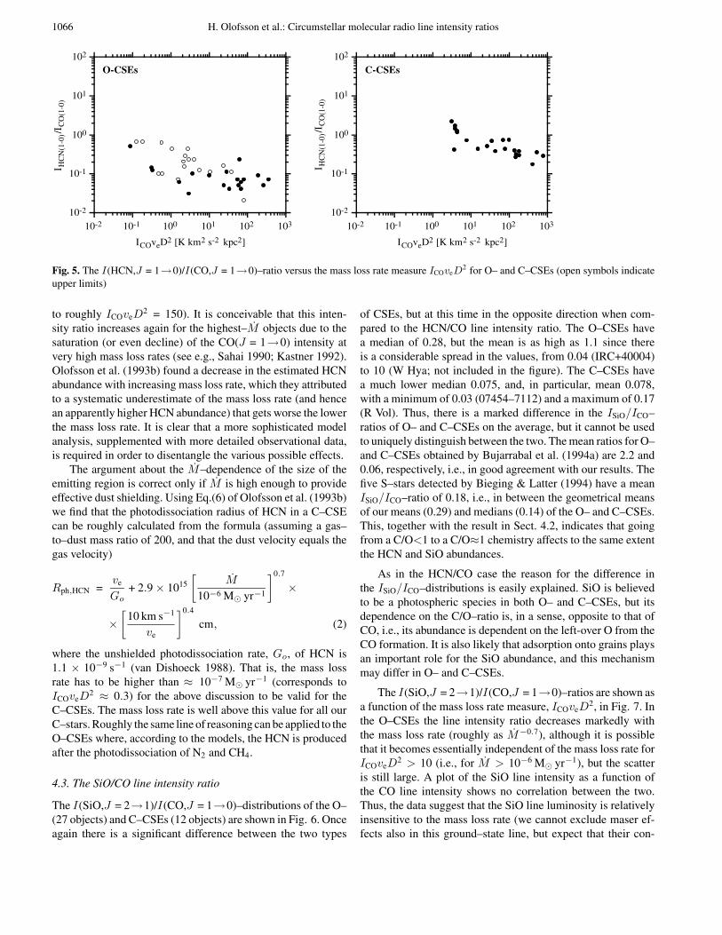
Fig. 5. The I(HCN,J = 1→0)/I(CO,J = 1→0)–ratio versus the mass loss rate measure ICOveD2 for O– and C–CSEs (open symbols indicate

upper limits)

to roughly ICOveD2 = 150). It is conceivable that this inten-

sity ratio increases again for the highest–M objects due to thesaturation (or even decline) of the CO(J = 1→0) intensity atvery high mass loss rates (see e.g., Sahai 1990; Kastner 1992).Olofsson et al. (1993b) found a decrease in the estimated HCNabundance with increasing mass loss rate, which they attributedto a systematic underestimate of the mass loss rate (and hencean apparently higher HCN abundance) that gets worse the lowerthe mass loss rate. It is clear that a more sophisticated modelanalysis, supplemented with more detailed observational data,is required in order to disentangle the various possible effects.

The argument about the M–dependence of the size of theemitting region is correct only if M is high enough to provideeffective dust shielding. Using Eq.(6) of Olofsson et al. (1993b)we find that the photodissociation radius of HCN in a C–CSEcan be roughly calculated from the formula (assuming a gas–to–dust mass ratio of 200, and that the dust velocity equals thegas velocity)

Rph,HCN =ve

Go+ 2.9× 1015

[M

10−6 M� yr−1

]0.7

×

×[

10 km s−1

ve

]0.4

cm, (2)

where the unshielded photodissociation rate, Go, of HCN is1.1 × 10−9 s−1 (van Dishoeck 1988). That is, the mass lossrate has to be higher than ≈ 10−7 M� yr−1 (corresponds toICOveD

2 ≈ 0.3) for the above discussion to be valid for theC–CSEs. The mass loss rate is well above this value for all ourC–stars. Roughly the same line of reasoning can be applied to theO–CSEs where, according to the models, the HCN is producedafter the photodissociation of N2 and CH4.

4.3. The SiO/CO line intensity ratio

The I(SiO,J = 2→1)/I(CO,J = 1→0)–distributions of the O–(27 objects) and C–CSEs (12 objects) are shown in Fig. 6. Onceagain there is a significant difference between the two types

of CSEs, but at this time in the opposite direction when com-pared to the HCN/CO line intensity ratio. The O–CSEs havea median of 0.28, but the mean is as high as 1.1 since thereis a considerable spread in the values, from 0.04 (IRC+40004)to 10 (W Hya; not included in the figure). The C–CSEs havea much lower median 0.075, and, in particular, mean 0.078,with a minimum of 0.03 (07454–7112) and a maximum of 0.17(R Vol). Thus, there is a marked difference in the ISiO/ICO–ratios of O– and C–CSEs on the average, but it cannot be usedto uniquely distinguish between the two. The mean ratios for O–and C–CSEs obtained by Bujarrabal et al. (1994a) are 2.2 and0.06, respectively, i.e., in good agreement with our results. Thefive S–stars detected by Bieging & Latter (1994) have a meanISiO/ICO–ratio of 0.18, i.e., in between the geometrical meansof our means (0.29) and medians (0.14) of the O– and C–CSEs.This, together with the result in Sect. 4.2, indicates that goingfrom a C/O<1 to a C/O≈1 chemistry affects to the same extentthe HCN and SiO abundances.

As in the HCN/CO case the reason for the difference inthe ISiO/ICO–distributions is easily explained. SiO is believedto be a photospheric species in both O– and C–CSEs, but itsdependence on the C/O–ratio is, in a sense, opposite to that ofCO, i.e., its abundance is dependent on the left-over O from theCO formation. It is also likely that adsorption onto grains playsan important role for the SiO abundance, and this mechanismmay differ in O– and C–CSEs.

The I(SiO,J = 2→1)/I(CO,J = 1→0)–ratios are shown asa function of the mass loss rate measure, ICOveD

2, in Fig. 7. Inthe O–CSEs the line intensity ratio decreases markedly withthe mass loss rate (roughly as M−0.7), although it is possiblethat it becomes essentially independent of the mass loss rate forICOveD

2 > 10 (i.e., for M > 10−6 M� yr−1), but the scatteris still large. A plot of the SiO line intensity as a function ofthe CO line intensity shows no correlation between the two.Thus, the data suggest that the SiO line luminosity is relativelyinsensitive to the mass loss rate (we cannot exclude maser ef-fects also in this ground–state line, but expect that their con-

H. Olofsson et al.: Circumstellar molecular radio line intensity ratios 1067

0

2

4

6

8

10

12

0 1 2 3 4 5

O-CSEs

No.

of

sour

ces

ISiO(2-1) /ICO(1-0)

0

2

4

6

8

10

12

0 0.1 0.2 0.3 0.4 0.5

C-CSEs

No.

of

sour

ces

ISiO(2-1) /ICO(1-0)

0

2

4

6

8

10

12

0 0.1 0.2 0.3 0.4 0.5

O-CSEsN

o. o

f so

urce

s

ISiO(2-1) /ICO(1-0)

Fig. 6. The I(SiO,J = 2→1)/I(CO,J =1→0)–distributions for O– (R Hya andW Hya with their line intensity ratios of6.9 and 10, respectively, are not includedin the figure) and C–CSEs. The distribu-tion of O–CSEs with a line intensity ratio<0.5 is shown below that of the C–CSEs

tribution to the line intensity is negligable, see e.g., Nyman &Olofsson 1985). A possible explanation to this is that the radiusof the SiO envelope is determined by grain adhesion, whichincreases with density, rather than photodissociation, which de-creases with density (cf. Sahai & Bieging 1993). This can bechecked by comparing the linear sizes [half–maximum inten-sity angular sizes from Lucas et al. (1992), assuming exponen-tial brightness distributions, scaled to the distances used in thispaper] of the SiO line–emitting regions of six of the stars in oursample (WX Psc, IK Tau, R Leo, W Hya, RX Boo, and R Cas)with the mass loss rate measure. The result is a very good cor-relation between the two, but the depencence on the mass lossrate measure is much weaker than that of for instance the HCNshell radius [the exponent is≈0.3, while for HCN the results ofNercessian et al. (1989) and Eq. (1) point to an exponent≈0.5, aresult in accordance with recent interferometer observations ofLindqvist et al. (priv. com.)]. However, as pointed out by Sahai& Bieging (1993) the angular sizes measured by Lucas et al.(1992) are surprisingly similar for all stars, suggesting that thebrightness distributions rather follow a scale–free power-law. Ifso, the correlation found is merely an effect of the different dis-tances to the sources. Possibly, the SiO excitation dependenceon the mass loss rate is of such a character that combined withother effects the SiO intensity becomes essentially independentof the mass loss rate.

It is difficult to establish whether or not there is any trend forthe C–CSEs since only the higher–M objects are detected, andthe upper limits for the low–M are not significant in comparisonwith these. We note here the peculiar line profile of the SiO(J =

2→1) line towards R Lep, which may indicate the presence ofmaser emission in this line (see Fig. 1). Similar, weak, and timevariable features have been seen towards O–CSEs (Nyman &Olofsson 1985).

4.4. The HCN/SiO line intensity ratio

The line intensity ratios discussed in the two previous sectionssuggest that the IHCN/ISiO–ratio should be a very good dis-criminator between O– and C–CSEs, since the HCN and SiOintensities show opposite trends with the C/O–ratio. Indeed,our data show a significant difference between the I(HCN,J =1→0)/I(SiO,J = 2→1)–distributions of the O– (19 objects)and C–CSEs (12 objects), Fig. 8. The former has a median valueof 0.28 and a maximum value of 0.46, while the latter has a me-dian value of 6.2 and a minimum value of 2.3 (note also thatnone of the lower limits is lower than this), i.e, the lowest C–CSE ratio is well above (by a factor of 5) the highest O–CSEratio, and the medians differ by a factor of 20. The difference isso large, compared to the uncertainties in the line intensity ratiosof the high–ratio O–CSEs and the low–ratio C–CSEs (estimatedto be less than 30%), that one can safely use this line intensityratio to distinguish between “normal” O– and C–CSEs. Thisresult is in perfect agreement with that obtained by Bujarrabalet al. (1994a,b). Their mean ratios for O– and C–CSEs are 0.28and 12.5. respectively, while we find 0.24 and 5.6, respectively.The difference for the C–CSEs is due to a few objects in theBujarrabal et al. sample that have very high IHCN/ISiO–ratios.The four S–stars detected in the HCN(J = 1→0) and SiO(J =

1068 H. Olofsson et al.: Circumstellar molecular radio line intensity ratios

10-2

10-1

100

101

102

10-2 10-1 100 101 102 103

O-CSEsI S

iO(2

-1)/

I CO

(1-0

)

ICOveD2 [K km2 s-2 kpc2]

10-2

10-1

100

101

102

10-2 10-1 100 101 102 103

C-CSEs

I SiO

(2-1

)/I

CO

(1-0

)

ICOveD2 [K km2 s-2 kpc2]

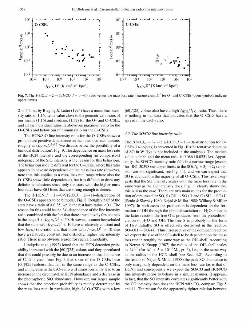
Fig. 7. The I(SiO,J = 2→1)/I(CO,J = 1→0)–ratio versus the mass loss rate measure ICOveD2 for O– and C–CSEs (open symbols indicate

upper limits)

2→1) lines by Bieging & Latter (1994) have a mean line inten-sity ratio of 1.16, i.e., a value close to the geometrical means ofour means (1.16) and medians (1.32) for the O– and C–CSEs,and all the individual ratios lie above our maximum ratio for theO–CSEs and below our minimum ratio for the C–CSEs.

The HCN/SiO line intensity ratio for the O–CSEs shows apronounced positive dependence on the mass loss rate measure,roughly as (ICOveD

2)0.3 (we discuss below the possibility of abimodal distribution), Fig. 9. The dependence on mass loss rateof the HCN intensity and the corresponding (in comparison)indepence of the SiO intensity is the reason for this behaviour.The behaviour is quite different for the C–CSEs, where this ratioappears to have no dependence on the mass loss rate (however,note that this applies to a mass loss rate range where also theO–CSEs show little dependence), but it is difficult to draw anydefinite conclusions since only the stars with the higher massloss rates have SiO lines that are strong enough to detect.

The I(HCN,J = 1→0)/I(SiO,J = 2→1)–distribution ofthe O–CSEs appears to be bimodal, Fig. 8. Roughly half of thestars have a ratio of≈0.35, while the rest have ratios <0.1. Thereason for this could be the M–dependence of the line intensityratio, combined with the fact that there are relatively few sourcesin the range 5 < ICOveD

2 < 50. However, it cannot be excludedthat the stars with ICOveD

2 < 10 have a relatively constant andlow IHCN/ISiO–ratio, and that those with ICOveD

2 > 10 alsohave a relatively constant, but distinctly, higher line intensityratio. There is no obvious reason for such a bimodality.

Lindqvist et al. (1992) found that the HCN detection prob-ability increased with the [60]/[25]-colour, and they speculatedthat this could possibly be due to an increase in the abundanceof C. It is clear from Fig. 3 that some of the O–CSEs have[60]/[25]-colours that fall in the same range as the C–CSEs,and an increase in the C/O–ratio will almost certainly lead to anincrease in the circumstellar HCN abundance and a decrease inthe photospheric SiO abundance. However, our larger sampleshows that the detection probability is mainly determined bythe mass loss rate. In particular, high–M O–CSEs with a low

[60]/[25]-colour also have a high IHCN/ISiO–ratio. Thus, thereis nothing in our data that indicates that the O–CSEs have aspread in the C/O–ratio.

4.5. The SO/CO line intensity ratio

The I(SO,JK = 32→21)/I(CO,J = 1→0)–distribution for O–CSEs (14 objects) is presented in Fig. 10 (the tentative detectionof SO in W Hya is not included in the analysis). The medianvalue is 0.09, and the mean ratio is 0.086±0.025 (1σ). Appar-ently, the SO/CO intensity ratio falls in a narrow range [exceptfor IRC–30398 our upper limits to the SO(JK = 32→21) emis-sion are not significant, see Fig. 11], and we can expect thatSO is abundant in the majority of all O–CSEs. This result sug-gests that the SO intensity scales with the mass loss rate in thesame way as the CO intensity does. Fig. 11 clearly shows thatthis is also the case. There are two main routes for the produc-tion of circumstellar SO, S+OH→ SO+H and O+SH→ SO+H(Scalo & Slavsky 1980; Nejad & Millar 1988; Willacy & Millar1997). In both cases the production is dependent on the for-mation of OH through the photodissociation of H2O, since inthe latter reaction the free O is produced from the photodisso-ciation of H2O and OH. The free S is probably in the formof H2S initially. SO is effectively destroyed in the reactionSO+OH→ SO2+H. Thus, irrespective of the dominant reactionwe expect the size of the SO–shell to be dependent on the massloss rate in roughly the same way as the OH–shell. Accordingto Netzer & Knapp (1987) the radius of the OH–shell scalesas M 0.7 (for M > 5 × 10−7 M� yr−1), i.e., in the same wayas the radius of the HCN–shell (see Sect. 4.2). According tothe results of Nejad & Millar (1988) the peak SO abundance isonly marginally dependent on the mass loss rate (as is that ofHCN), and consequently we expect the SO/CO and HCN/COline intensity ratios to behave in a similar manner. It appears,in fact, that the SO intensity correlates significantly better withthe CO intensity than does the HCN with CO, compare Figs 5and 11. The reason for the apparently tighter relation between

H. Olofsson et al.: Circumstellar molecular radio line intensity ratios 1069

0

2

4

6

8

0 0.2 0.4 0.6 0.8 1

O-CSEsN

o. o

f so

urce

s

IHCN(1-0) /ISiO(2-1)

0

2

4

6

8

0 2 4 6 8 10

C-CSEs

No.

of

sour

ces

IHCN(1-0) /ISiO(2-1)

Fig. 8. The I(HCN,J = 1→0)/I(SiO,J = 2→1)–distributions for O– and C–CSEs

10-2

10-1

100

101

102

10-2 10-1 100 101 102 103

O-CSEs

I HC

N(1

-0)/

I SiO

(2-1

)

ICOveD2 [K km2 s-2 kpc2]

10-2

10-1

100

101

102

10-2 10-1 100 101 102 103

C-CSEsI H

CN

(1-0

)/I S

iO(2

-1)

ICOveD2 [K km2 s-2 kpc2]

Fig. 9. The I(HCN,J = 1→0)/I(SiO,J = 2→1)–ratio versus the mass loss rate measure ICOveD2 for O– and C–CSEs (open symbols indicate

upper limits for O–CSEs and lower limits for C–CSEs)

the SO and CO intensities is not clear, but it can be due to bothchemistry and excitation. The former very likely plays a rolesince the SO abundance is dependent on the H2O abundance,while the HCN abundance is dependent on the abundance of thefree C (due to photodissociation of CH4, which in itself has tobe produced in the inner CSE according to the models), whichpresumably can vary substantially. Also, the outer radius of theHCN–shell is determined by photodissociation, while the outerradius of the SO–shell depends on the chemical destruction (seeabove).

We have not attempted to detect SO towards C–CSEs. Bu-jarrabal et al. (1994a) failed to do so despite a relatively sensitivesearch towards a few objects.

We have not detected the higher-lying (in energy), but inher-ently weaker, SO(JK = 22→11) line (the 32 and 22 levels haveenergies of 9.2 and 19.3 K, respectively). SO has a 3Σ groundstate, and the rotational energy levels can be divided into threegroups (J = N − 1, J = N , and J = N + 1, where J and Nare the total and rotational angular momentum quantum num-

bers in the pure Hund’s coupling case b, respectively). Radiativetransitions between the groups are very weak compared to tran-sitions within the groups (except for the lowerJ-values), and wetherefore expect the excitation between the groups to be largelydetermined by collisions. The upper limits to the SO(22 → 11)line are low and indicate a kinetic temperature below 20 K inthe SO line–emitting region.

4.6. Line intensity ratios involving CS and SiS

The detections of CS and SiS in O–CSEs are so few that wewill only briefly discuss the most interesting line intensity ra-tios involving these species. We have detected only two O–CSEsin CS (three more O–CSEs of AGB–stars have been detectedin CS: WX Psc, RX Boo, and IRC–10529, Bujarrabal et al.1994a), and only three O–CSEs in SiS (one more O–CSE hasbeen detected in SiS: IRC–10529, Bujarrabal et al. 1994a). Itis obvious that only tentative conclusions can be drawn fromthese data. We present the results as I(CS,J = 2→1)/I(CO,J =1→0)–, I(SiS,J = 5→4)/I(CO,J = 1→0)–, and I(SiS,J =

1070 H. Olofsson et al.: Circumstellar molecular radio line intensity ratios

0

2

4

6

8

10

0 0.05 0.1 0.15 0.2

O-CSEsN

o. o

f so

urce

s

ISO(3,2-2,1)/ICO(1-0)

Fig. 10. The I(SO,JK = 32→21)/I(CO,J = 1→0)–distribution forO–CSEs

10-2

10-1

100

101

102

10-2 10-1 100 101 102 103

O-CSEs

I SO

(3,2

-2,1

)/I C

O(1

-0)

ICOveD2 [K km2 s-2 kpc2]

Fig. 11. The I(SO,JK = 32→21)/I(CO,J = 1→0)–ratio versus themass loss rate measure ICOveD

2 for O–CSEs (open symbols indicateupper limits)

5→4)/I(SiO,J = 2→1)–distributions for the O– and C–CSEsin Figs 12, 13, and 14. The upper limits for the O–CSEs are notsignificant.

The mean I(CS,J = 2→1)/I(CO,J = 1→0)–ratio of theO–CSEs, 0.029, is much lower than that of the C–CSEs, 0.24.However, it is clear already from this limited data set that this lineintensity ratio does not provide a clear discrimination betweenO– and C–CSEs, since there is a pronounced tail of low ratios forthe C–CSEs. The difference in the ICS/ICO–distributions is ex-pected also from theory. In an O–CSE the CS molecules are pro-duced in the envelope via the reactions starting with C++H2S orS++CH leading to the formation of HCS+, which dissociativelyrecombines with an electron or proton transfers with NH3, orvia the reactions C+SO→CS+O and C+SH→CS+H (Nejad &Millar 1988; Willacy & Millar 1997). The predicted abundances(few× 10−7) are in all cases much lower than the expected CSabundance in a C–CSE. In the latter case the observed CS is be-

lieved to be of photospheric origin, and Olofsson et al. (1993a)derived a maximum abundance of ≈ 3 × 10−5. However, thephotospheric CS abundance is rather sensitive to temperature(and to some extent the C/O–ratio) and abundances as low as≈10−8 are possible. This probably explains the tail toward lowICS/ICO–ratios for the C–CSEs.

The mean I(SiS,J = 5→4)/I(CO,J = 1→0)–ratio of theO–CSEs, 0.02, is lower than that of the C–CSEs, 0.041 (notethat this value applies to relatively high–M objects), but eventhis limited data set shows that this line intensity ratio can notbe used as a discriminator. In an O–CSE the SiS is probablya photospheric species [and possibly additionally produced inthe envelope through the reaction S++SiH→ SiS+H+ if graindepletion of Si is negligable, Scalo & Slavsky (1980)], and thecalculated SiS/SiO abundance ratio is ≈0.1 (Tsuji 1973). In aC–CSE the SiS is also believed to be of photospheric origin,and its predicted abundance (≤ 3× 10−5) is relatively insensi-tive to temperature and C/O-ratio (Olofsson et al. 1993b). Thecalculated SiS/SiO abundance ratios is >∼1 in this case. Thus,considering that the SiO/CO line intensity ratio is 5–10 timeshigher in O–CSEs than in C–CSEs, the small difference in theISiS/ICO–distributions is not unexpected.

The mean I(SiS,J = 5→4)/I(SiO,J = 2→1)–ratio of theC–CSEs is about 10 times higher than that of the O–CSEs,i.e., the average line intensity ratio difference agrees with theexpected abundance ratio difference. Despite this, this line in-tensity ratio is not a perfect discriminator since, for unknownreason, some C–CSEs are very weak in the SiS(J = 5→4) line.The C–CSEs are divided into a low– and a high–ratio group,but this could be an effect of too poor statistics.

Line intensity ratios of further interest to compare areCS/HCN, CS/SiS, and CS/SO. CS and HCN have the sameorigins in O– and C–CSEs, but they differ between the twochemistries, i.e., they are circumstellar in O–CSEs and pho-tospheric in C–CSEs. The mean I(CS,J = 2→1)/I(HCN,J =1→0)–ratio is 0.17 in O–CSEs, while for the C–CSEs the ratioscentre around ≈0.6, but with a substantial tail towards valueslower than 0.1. The mean I(CS,J = 2→1)/I(SiS,J = 5→4)–ratios are 1.7 and 10 in O– and C–CSEs, respectively. None ofthese line intensity ratios are likely to be good discriminators be-tween O– and C–CSEs. The mean I(CS,J = 2→1)/I(SO,JK =32→21)–ratio in O–CSEs is 0.3.

4.7. Anomalous line intensity ratios and peculiar sources

The results based on line intensity ratios presented in the previ-ous sections apply only to “normal” CSEs. By “normal” in thiscontext we mean a CSE formed by a relatively constant mass lossrate (both in magnitude and chemical composition) over a periodlonger than the time required to substantially change the densitystructure or the composition of the gas within the line emittingregions, <∼103 years, i.e., on intermediate time scales. A rapidchange in the chemical composition of the ejected gas or in themass loss rate would eventually lead to anomalous line intensityratios. In the former case, we expect the CSE to show a chemistrydifferent from that expected from the chemical composition of

H. Olofsson et al.: Circumstellar molecular radio line intensity ratios 1071

0

2

4

6

8

0 0.1 0.2 0.3 0.4 0.5

detection

upper limit

O-CSEs

ICS(2-1) /ICO(1-0)

No.

of

sour

ces

0

2

4

6

8

0 0.1 0.2 0.3 0.4 0.5

detection

upper limit

C-CSEs

ICS(2-1) /ICO(1-0)

No.

of

sour

ces

Fig. 12. The I(CS,J = 2→1)/I(CO,J = 1→0)–distributions for O– and C–CSEs

0

2

4

6

8

0 0.05 0.1 0.15 0.2

detection

upper limit

O-CSEs

No.

of

sour

ces

ISiS(5-4) /ICO(1-0)

0

2

4

6

8

0 0.05 0.1 0.15 0.2

detection

upper limit

C-CSEs

No.

of

sour

ces

ISiS(5-4) /ICO(1-0)

Fig. 13. The I(SiS,J = 5→4)/I(CO,J = 1→0)–distributions for O– and C–CSEs

0

2

4

6

8

0 0.4 0.8 1.2 1.6 2

detection

upper limit

O-CSEs

No.

of

sour

ces

ISiS(5-4) /ISiO(2-1)

0

2

4

6

8

0 0.4 0.8 1.2 1.6 2

detection

upper limit

C-CSEs

No.

of

sour

ces

ISiS(5-4) /ISiO(2-1)

Fig. 14. The I(SiS,J = 5→4)/I(SiO,J = 2→1)–distributions for O– and C–CSEs

1072 H. Olofsson et al.: Circumstellar molecular radio line intensity ratios

the central star. We find no evidence for such a situation in anyof the objects observed, e.g., a high (low) IHCN/ISiO–ratio in aCSE around an M–star (C–star). In the latter case, the emissionfrom molecular species excited at different radii may behave dif-ferently, e.g., a recent decrease in the mass loss rate decreasesthe emission from molecules excited close to the star while theCO emission is hardly affected. Interesting examples of this areprovided by the carbon star R Scl, which, due to a probably re-cently detached CSE, shows a low I(HCN,J = 1→0)/I(CO,J =1→0)–ratio and a high I(CN,N = 1→0)/I(HCN,J = 1→0)–ratio, and the carbon stars U Ant, S Sct, and TT Cyg with clearlydetached shells, which show very low upper limits to a num-ber of I(X,j → i)/I(CO,J = 1→0)–ratios (Bujarrabal & Cer-nicharo 1994; Olofsson et al. 1996). Once again, we find no lineintensity ratios that indicate significant mass loss rate variationson intermediate time scales for our objects.

However, there is one source in our sample with an appar-ently non–normal CSE [the C–star U Cam appears to have a de-tached shell (Lindqvist et al. 1996)], which despite this exhibitsno obviously anomalous line intensity ratios. This shows thatline intensity ratios do not unambiguously identify CSEs withnon–normal characteristics. Furthermore, the M–star W Hyashows a high I(HCN,J = 1→0)/I(CO,J = 1→0)–ratio, and,in particular, a very high I(SiO,J = 2→1)/I(CO,J = 1→0)–ratio compared to the other M–stars [the latter ratio is high alsofor R Dor and R Hya]. We have no obvious explanation of this.

5. HCN(J = 1→0) masers in C–CSEs

The existence of strong HCN masers associated with carbonstars was discovered accidentally when searching for HCO+(J =1→0) emission towards C–CSEs (Guilloteau et al. 1987).The masing J = 1→0 transition lies in the vibrationally ex-cited state (0,20,0) about 2050 K above the ground state. Lu-cas et al. (1988) showed that this maser is not uncommon,but it appears to be restricted to a limited mass loss rate range(≈10−6 − 10−5 M� yr−1). Subsequently, Lucas & Cernicharo(1989) detected another strong HCN maser. In this case itwas the J = 2→1 transition in the vibrationally excited state(0,11c ,0). In IRC+10216, the archetype of C–CSEs, they alsoobserved all possible J = 1→0, 2→ 1, and 3→ 2 transitionsin the fundamental and two lowest–lying vibrational states ofHCN, and inferred that a pump mechanism similar to that of thestrong SiO masers associated with M–stars is quite possible.

The presence of ground–state J = 1→0 maser emissionwas first noticed by Izumiura et al. (1987) [see also Izumiura(1990) and Olofsson et al. (1993b)]. The maser emission natureis inferred from the presence of time–variable narrow features.It appears not to be a question of strong masers, but it makesthe estimate of the HCN abundance uncertain, and it adds fur-ther evidence that the excitation of circumstellar HCN is quitecomplicated. The vibrationally excited strong masers almostcertainly lie very close to the star (Carlstrom et al. 1990; Lucas& Guilloteau 1992). For the ground–state masers the situation isunclear. We have therefore performed a time monitoring studyof the HCN(J = 1→0) emission from two bright carbon stars,

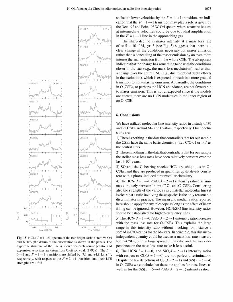
W Ori (semiregular variable, P≈210 days) and X TrA (irreg-ular variable). The spectra are presented in Fig. 15. The totalintegrated fluxes of the two sources vary irregularly with timeat levels that are not significant when the calibration uncertaintyis taken into account. For both sources the line consists of twocomponents: a broad emission which covers roughly the samevelocity range as the CO(1→ 0) emission [data from Olofssonet al. (1993a)], and narrow features that predominantly appearat the blue– and redshifted edges of the emission. The redshiftedfeature lies somewhat closer to the systemic velocity than the,more rarely occurring, blueshifted feature, and it is in generalstronger, a conclusion also reached by Izumiura et al. (1995) forW Ori and Y CVn (a J–type carbon star).

The CN observations of Bachiller et al. (1997) show anoma-lous I(CN,N = 2→1)/I(HCN,J = 1→0)–ratios for W Ori,UU Aur, and Y CVn, further emphasizing the possible impor-tance of maser action in the HCN(J = 1→0) line. However, thesituation appears even more complicated since a comparison ofCN(N = 1→0) and CN(N = 2→1) intensities suggests maseraction in the CN(N = 2→1) line in W Ori and UU Aur.

The interpretation of the HCN(J = 1→0) data is made dif-ficult by the hyperfine structure of the J=1 level, which resultsin three lines that are shifted in velocity with respect to eachother by an amount that is usually lower than the expansionvelocity of the CSE. Hence, the line profile consists of threeblended lines, see Fig. 15, and the radiative transfer becomescomplicated (Truong–Bach & Nguyen–Q–Rieu 1989).

We find comparatively very little HCN(J = 1→0) emis-sion outside the velocity range of the CO emission for bothstars (on average <∼10% of the total intensity), showing thatthe approaching (receding) material emits very little in the F =0→1 (F = 1→1) transition. This indicates that the emissionis dominated by the F = 2→1 line. Furthermore, the strongredshifted feature cannot be due to the F = 0→1 component(assuming that no gas with velocities outside the CO range ex-ists). Likewise, the blueshifted feature that occasionally appearscannot be due to the F = 1→1 component. On the other hand,the red– and blueshifted features can be due to gas at roughlythe systemic velocity emitting in the F = 1→1 and F = 0→1component, respectively. The red- and blueshifted features canequally well be due to receding and approaching gas emittingin the F = 2→1 line, i.e., a structure similar to that of an OH1612 MHz maser, although the symmetry around the systemicvelocity is not perfect here. The F = 1→1 emission goes un-affected through the envelope. The redshifted part of the F =2→1 emission can be absorbed or amplified in the F = 1→1transition, and if the latter is inverted this may cause a strongmaser feature that appear somewhere at intermediate redshiftedvelocities. The blueshifted F = 2→1 emission is unaffected,and if there is radial amplification the blue maser feature shouldappear at the blueshifted edge of the CO emission. The samething happens to the F = 0→1 emission except that it becomesaffected also by the F = 2→1 transition. This discussion sug-gests that the most reasonable explanation to the data, althoughby no means unique, is radial amplification in the F = 2→1line, and the redshifted feature may be further amplified and

H. Olofsson et al.: Circumstellar molecular radio line intensity ratios 1073

Fig. 15. HCN(J = 1→0) spectra of the two bright carbon stars W Oriand X TrA (the datum of the observation is shown in the panel). Thehyperfine structure of the line is shown for each source [centre andexpansion velocities are taken from Olofsson et al. (1993a)]. The F =0→1 and F = 1→1 transitions are shifted by -7.1 and +4.8 km s−1,respectively, with respect to the F = 2→1 transition, and their LTEstrengths are 1:3:5

shifted to lower velocities by the F = 1→1 transition. An indi-cation that the F = 1→1 transition may play a role is given bythe Dec.–92 and Febr.–93 W Ori spectra where a narrow featureat intermediate velocities could be due to radial amplificationin the F = 1→1 line in the approaching gas.

The sharp decline in maser intensity at a mass loss rateof ≈ 5 × 10−7 M� yr−1 (see Fig. 5) suggests that there is aclear change in the conditions necessary for maser emissionrather than a concealing of the maser emission by an even moreintense thermal emission from the whole CSE. The abruptnessindicates that the change has something to do with the conditionscloser to the star (e.g., the mass loss mechanism), rather thana change over the entire CSE (e.g., due to optical depth effectsin the excitation), which is expected to result in a more gradualtransition to non–masing emission. Apparently, the conditionsin O–CSEs, or perhaps the HCN abundance, are not favourableto maser emission. This is not unexpected since if the modelsare correct there are no HCN molecules in the inner region ofan O–CSE.

6. Conclusions

We have utilized molecular line intensity ratios in a study of 39and 22 CSEs around M– and C–stars, respectively. Our conclu-sions are:1) There is nothing in the data that contradicts that for our samplethe CSEs have the same basic chemistry (i.e., C/O<1 or >1) asthe central stars.2) There is nothing in the data that contradicts that for our samplethe stellar mass loss rates have been relatively constant over thelast <∼103 years.3) SO and the C–bearing species HCN are ubiquitous in O–CSEs, and they are produced in quantities qualitatively consis-tent with a photo–induced circumstellar chemistry.4) The HCN(J = 1→0)/SiO(J = 2→1) intensity ratio discrimi-nates uniquely between “normal” O– and C–CSEs. Consideringalso the strength of the various circumstellar molecular lines itis clear that a ratio involving these species is the only reasonablediscriminator in practice. The mean and median ratios reportedhere should apply for any telescope as long as the effect of beamfilling can be ignored. However, HCN/SiO line intensity ratiosshould be established for higher–frequency lines.5) The HCN(J = 1→0)/SiO(J = 2→1) intensity ratio increaseswith the mass loss rate for O–CSEs. This explains the largerange in this intensity ratio without invoking for instance aspread in C/O–ratios for the M–stars. In principle, this distance–independent quantity could be used as a mass loss rate measurefor O–CSEs, but the large spread in the ratio and the weak de-pendence on the mass loss rate make it less useful.6) The HCN(J = 1→0) and SiO(J = 2→1) intensity ratioswith respect to CO(J = 1→0) are not perfect discriminators.Despite the few detections of CS(J = 2→1) and SiS(J = 5→4)in O–CSEs we conclude that the same applies for these lines, aswell as for the SiS(J = 5→4)/SiO(J = 2→1) intensity ratio.

1074 H. Olofsson et al.: Circumstellar molecular radio line intensity ratios

7) The SO(JK = 32→21) and CO(J = 1→0) intensities aretightly correlated, suggesting that SO lines may be used as goodmass loss rate estimators.8) The HCN(J = 1→0) line exhibits maser features in low-MC–CSEs. We suggest that the strongest maser features are dueto radial amplification in theF = 2→1 transition, with possiblyadditional radial amplification in the F = 1→1 transition.

Acknowledgements. We are grateful to Franz Kerschbaum for supply-ing us with distances to the M–stars. The Swedish-ESO SubmillimetreTelescope, SEST, is operated jointly by ESO and the Swedish NationalFacility for Radio Astronomy, Onsala Space Observatory at ChalmersUniversity of Technology. Financial support from the Swedish NaturalScience Research Council (NFR) is acknowledged.

References

Bachiller R. Fuente A., Bujarrabal V., et al. 1997 A&A 319, 235Bedijn P.J. 1987, A&A 186, 136Benson P.J., Little–Marenin I.R., Woods T.C., et al. 1990, ApJS 74,

911Bieging J.H., Latter W.B. 1994, ApJ 422, 765Bujarrabal V., Cernicharo J. 1994, A&A 288, 551Bujarrabal V., Fuente A., Omont A. 1994a, A&A 285, 247Bujarrabal V., Fuente A., Omont A. 1994b, ApJ 421, L47Carlstrom J.E., Welch W.J., Goldsmith P.F., Lis D.C. 1990, AJ 100,

213Charnley S.B., Latter W.B. 1997, MNRAS 287, 538Charnley S.B., Tielens A.G.G.M., Kress M.E. 1995, MNRAS 274, L53Cherchneff I., Barker J.R. 1992, ApJ 394, 703Cherchneff I., Glassgold A.E. 1993, ApJ 419, L41Engels D., Heske A. 1989, A&AS 81, 323Glassgold A.E., Huggins P.J. 1983, MNRAS 203, 517Glassgold A.E., Omont A., Guelin M. 1992, ApJ 396, 115Groenewegen M.A.T. 1994, A&A 290, 531Groenewegen M.A.T., Baas F., de Jong T., Loup C. 1996, A&A 306,

241Guilloteau S., Omont A., Lucas R. 1987, A&A 176, L24Huggins P.J., Glassgold A.E. 1982, ApJ 252, 201Izumiura H. 1990, PhD Thesis, Tokyo UniversityIzumiura H., Ukita N., Kawabe R., et al. 1987, ApJ 323, L81Izumiura H., Ukita N., Tsuji T. 1995, ApJ 440, 728Justtanont K., Skinner C.J., Tielens A.G.G.M. 1994, ApJ 435, 852Kahane C., Jura M. 1994, A&A 290, 183Kastner J.H. 1992, ApJ 401, 337Kerschbaum F., Hron J. 1996, A&A 308, 489Kerschbaum F., Olofsson H., Hron J. 1996, A&A 311, 273Kholopov P.N., et al. 1985, General Catalogue of Variable Stars, 4:th

ed., Moscow Publishing House, MoscowKwan J., Webster Z. 1993, ApJ 419, 674Lafont S., Lucas R., Omont A. 1982, A&A 106, 201Lambert D.L., Gustafsson B., Eriksson K., Hinkle K.H. 1986, ApJS

62, 373Larsen F., Olofsson H., Eriksson K., Gustafsson B. 1997, in prep.Lindqvist M., Lucas R., Olofsson H., Omont A., Eriksson K., Gustafs-

son B. 1996, A&A 305, L57Lindqvist M., Nyman L-A., Olofsson H., Winnberg A. 1988, A&A

205, L15Lindqvist M., Olofsson H., Winnberg A., Nyman L-A. 1992, A&A

263, 183Loup C., Forveille T., Omont A. Paul J.F. 1993, A&AS 99, 291

Lucas R., Bujarrabal V., Guilloteau S., et al. 1992, A&A 262, 491Lucas R., Cernicharo J. 1989, A&A 218, L20Lucas R., Guilloteau S. 1992, A&A 259, L23Lucas R., Guilloteau S., Omont A. 1988, A&A 194, 230Millar T.J., Herbst E. 1994, A&A 288, 561Millar T.J., Olofsson H. 1993, MNRAS 262, L55Nejad L.A.M., Millar T.J. 1987, A&A 183, 279Nejad L.A.M., Millar T.J. 1988, MNRAS 230, 79Nercessian E., Guilloteau S., Omont A., Benayoun J.J. 1989, A&A

210, 225Netzer N., Knapp G.R. 1987, ApJ 323, 734Nyman L.-A., Booth R.S., Carlstrom U., et al. 1992, A&AS 93, 121Nyman L.-A., Olofsson H. 1985, A&A 150, 169Nyman L.-A., Olofsson H. 1997, in prep.Nyman L.-A., Olofsson H., Johansson L.E.B., Booth R.S., Carlstrom

U., Wolstencroft R., et al. 1993, A&A 269, 377Olnon F.M., Raymond E., eds of IRAS LRS Atlas, 1986, A&ASS 65,

607Olofsson H. 1997a, The Neutral Envelopes around AGB and Post–AGB

Objects: Circumstellar Molecules. In: van Dishoeck E.F. (ed.) Proc.IAU Symp. 178, Molecular Astrophysics: Probes & Processes.Kluwer, Dordrecht, p. 457

Olofsson H. 1997b, ApSS, 245, 169Olofsson H. 1997c, The Neutral Envelopes around AGB and Post–AGB

Objects: Their Structure and Evolution. In: Wing R. (ed.) Proc. IAUSymp. 177, The Carbon Star Phenomenon. Kluwer, Dordrecht, inpress

Olofsson H., Bergman P., Eriksson K., Gustafsson B. 1996, A&A 322,587

Olofsson H., Eriksson K., Gustafsson B., Carlstrom U. 1993a, ApJS87, 267

Olofsson H., Eriksson K., Gustafsson B., Carlstrom U. 1993b, ApJS87, 305

Olofsson H., Lindqvist M., Nyman L–A., Winnberg A., Nguyen–Q–Rieu 1991, A&A 245, 611

Omont A., Lucas R., Morris M., Guilloteau S. 1993, A&A 267, 490Sahai R. 1990, ApJ 362, 652Sahai R., Bieging J.H. 1993, AJ 105, 595Sahai R., Wannier P.G. 1992, ApJ 394, 320Scalo J.M, Slavsky D.B. 1980, ApJ 293, L73Sopka R.J., Olofsson H., Johansson L.E.B., Nguyen–Q–Rieu, Zucker-

man B. 1989, A&A 210, 78Truong–Bach, Nguyen–Q–Rieu 1989, A&A 214, 267Tsuji T. 1964, Ann. Tokyo Astron. Obs., 2nd ser. 9, 1Tsuji T. 1973, A&A 23, 411van der Veen W.E.C.J., Habing H.J, 1988, A&A 194, 125van der Veen W.E.C.J., Rugers M. 1989, A&A 226, 183van Dishoeck E.F. 1988, Photodissociation and Photoionization Pro-

cesses. In T.J. Millar and D.A. Williams (eds) Rate Coefficients inAstrochemistry. Kluwer, Dordrecht, p. 49

Whitelock P., Menzies J., Feast M., et al. 1994, MNRAS 267, 711Willacy K., Millar T.J. 1997, A&A 324, 237

This article was processed by the author using Springer-Verlag LaTEXA&A style file L-AA version 3.