Circulation anomalies in boreal winter: Origin of ...
85
Circulation anomalies in boreal winter: Origin of variability and trends during the ERA-40 period Diploma Thesis written by Gereon Gollan <[email protected]> IFM-Geomar Kiel Kiel, December 13, 2011
Transcript of Circulation anomalies in boreal winter: Origin of ...

Circulation anomalies in borealwinter: Origin of variability andtrends during the ERA-40 period
Diploma Thesis written by
Gereon Gollan<[email protected]>
IFM-Geomar Kiel
Kiel, December 13, 2011


Contents
Abstract iii
Zusammenfassung v
Acronyms vii
1 Introduction and motivation 1
2 Data and model 32.1 The ERA-40 reanalysis . . . . . . . . . . . . . . . . . . . . . . 32.2 The model . . . . . . . . . . . . . . . . . . . . . . . . . . . . . 5
2.2.1 Experiments . . . . . . . . . . . . . . . . . . . . . . . 92.3 NAO and NAM . . . . . . . . . . . . . . . . . . . . . . . . . . 122.4 PNA . . . . . . . . . . . . . . . . . . . . . . . . . . . . . . . . 16
3 Methods 193.1 Regression and correlation . . . . . . . . . . . . . . . . . . . . 193.2 Weighting and projection . . . . . . . . . . . . . . . . . . . . 203.3 EOF analysis . . . . . . . . . . . . . . . . . . . . . . . . . . . 213.4 Pattern correlation . . . . . . . . . . . . . . . . . . . . . . . . 233.5 Monte Carlo methods . . . . . . . . . . . . . . . . . . . . . . 24
4 Results 274.1 Seasonal forecasting . . . . . . . . . . . . . . . . . . . . . . . 29
4.1.1 NAO/NAM . . . . . . . . . . . . . . . . . . . . . . . . 324.1.2 PNA . . . . . . . . . . . . . . . . . . . . . . . . . . . . 42
4.2 Trends during the ERA-40 period . . . . . . . . . . . . . . . . 484.2.1 NAO/NAM . . . . . . . . . . . . . . . . . . . . . . . . 524.2.2 PNA . . . . . . . . . . . . . . . . . . . . . . . . . . . . 55
5 Conclusions and discussion 59
List of Figures 63
List of Tables 65
i

ii CONTENTS
Bibliography 67
Acknowledgements 73
Erklarung 75

Abstract
In this diploma thesis the interannual variability and trends of the wintermean tropospheric circulation in the northern hemisphere (NH) extratropicsin winters from 1960/61 to 2001/02 are investigated. Output is analysedfrom a recent version of the atmospheric ECMWF model that has beenused to perform various hindcast experiments, including experiments withselected regions of the atmosphere relaxed toward reanalysis data (ERA-40), i.e., the tropics and the stratosphere. The results are compared withthe reanalysis data to examine the forecasting skill of the single experimentsin the NH extratropics.
It is found that the stratosphere is influential on the interannual vari-ability of the North Atlantic Oscillation (NAO) related part of the win-ter tropospheric circulation variability in the North Atlantic sector (NAS),but less important for other modes of variability in the NAS or over theNorth Pacific sector (NPS). The influence of the stratosphere on the NAOis thought to be caused by the downward propagation of circulation anoma-lies, for example, caused by sudden stratospheric warmings. Relaxing thetropical atmosphere is influential for the general circulation variability in theNAS, although the influence on the NAO is somewhat smaller than relaxingthe global stratosphere. Both regions of the atmosphere therefore are im-portant for a seasonal forecast in the NAS in winter. In the case of tropicalrelaxation, adding prescribed observed sea surface temperatures and sea ice(SSTSI) from reanalysis data improves the representation of the NAO in themodel and is even more influential in reproducing the observed 42 year trendto a more positive NAO index. The stratosphere has a significant impact onthe observed positive NAO trend only between 1964/65 and 1994/95, and inthis period is comparable with the other forcings, the tropics and observedSSTSI. However, our model experiments are not able to account for morethan 25% of the interannual variance of the NAO and not for more than40% of the observed trend of the NAO in the ensemble means.
In the NPS the tropical atmosphere clearly has a strong impact on theinterannual variability, and hence the seasonal predictability, which is mea-sured here by means of the Pacific North America (PNA) pattern index.Single realisations of model experiments with tropical relaxation represent,on average, between 40% and 50% of the variance of the observed PNA pat-
iii

iv Abstract
tern. The ensemble mean with SSTSI from reanalysis data and no relaxationcaptures about 25% of the interannual variance of the observed PNA, butleads to a wrong trend in the PNA between 1960/61 and 2001/02 comparedwith the observations. The observed trend of the PNA is well captured interms of the trend pattern if the tropics are relaxed to reanalysis data, ex-cept that the magnitude of the trend is reduced in the ensemble mean. Itis remarkable that the observed PNA trend between 1960/61 and 2001/02is also found to be within the range of trends of a control experiment, thatsees the climatological mean cycles of SSTSI only. The strong impact of thetropical atmosphere on the extratropical atmosphere in the NPS is associ-ated to the strong link between El Nino related variability in the tropicalPacific and the PNA that was confirmed by a number of previous studies.

Zusammenfassung
In dieser Diplomarbeit werden die zwischenjahrliche Variabilitat und Trendsder mittlerenWinterzirkulation in der Troposphare der extratropischen Nord-hemisphare (NH) in Wintern von 1960/61 bis 2001/02 untersucht. Modell-ergebnisse von Hindcast Experimenten werden analysiert, die mit einer ak-tuelle Version des atmospharischen ECMWF Modells durchgefuhrt wurden,unter anderem Relaxationsexperimente, in denen ausgesuchte Regionen derAtmosphare, die Tropen und die Stratosphare, an Reanalysedaten (ERA-40) angeglichen wurden. Die Ergebnisse werden dann mit Reanalysedatenverglichen, um die Vorhersagegute der einzelnen Experimente in den Extra-tropen der NH zu bewerten.
Es wird herausgefunden, dass die Stratosphare Einfluss auf die zwischen-jahrliche Variabilitat der der Nord Atlantischen Oszillation (NAO) assozi-ierten Winterzirkulation im Nord Atlantischen Sektor (NAS) hat, jedochweniger wichtig fur andere Moden der Variabilitat im NAS oder im Nord-Pazifischen Sektor (NPS) ist. Der Einfluss der Stratosphare auf die NAOwird auf die Abwartspropagation von Zirkulationsanomalien zuruckgefuhrt,die zum Beispiel durch plotzliche Erwarmungen der Stratosphare (SSW)verursacht werden. Die tropische Atmosphare hat Einfluss auf die allgemeineVariabilitat der Zirkulation im NAS, ist jedoch fur die NAO Variabilitatweniger wichtig als die Statosphare. Beide Regionen der Atmosphare sinddaher im Winter wichtig fur eine saisonale Vorhersage im NAS. Im Falle dertropischen Relaxation verbessert das Vorschreiben von Meeresoberflachen-temperaturen und Meereisdaten (SSTSI) aus Reanalysedaten deutlich dieReprasentation der NAO im Modell und hat noch großeren Einfluss aufdie Reproduktion des beobachteten 42-Jahres Trends zwischen 1960/61 und2001/02 hin zu einem positiveren NAO Index. Die Stratosphare hingegenhat nur zwischen 1964/65 und 1994/95 einen signifikanten Einfluss auf denpositiven Trend der NAO, der dann mit dem Einfluss der anderen Forcings,den Tropen und SSTSI, vergleichbar ist. Unsere Modellexperimente konnenallerdings im Ensemblemittel nicht mehr als 25% der zwischenjahrlichenVariabilitat der NAO und nicht mehr als 40% des beobachteten Trendswiedergeben.
Im NPS hat die tropische Atmosphare einen deutlichen und starken Ein-fluss auf die zwischenjahrliche Variabilitat, und damit die saisonale Vorher-
v

vi Zusammenfassung
sagbarkeit, hier gemessen am Index des Pazifik-Nordamerika (PNA) Musters.Einzelne Modelllaufe mit tropischer Relaxation geben im Durchschnitt zwi-schen 40% und 50% der Varianz des beobachteten PNA Musters wieder.Mit vorgeschriebenen SSTSI aus Reanalysedaten und ohne Relaxation gibtdas Ensemblemittel 25% der zwischenjahrlichen Varianz der beobachtetenPNA wieder, liefert jedoch einen, verglichen mit den Beobachtungen, um-gekehrten Trend zwischen 1960/61 und 2001/02. Der beobachtete PNATrend hinsichtlich des Trendmusters wird mit tropischer Relaxation gut er-fasst, nur die Amplitude des beobachteten Trends wird nicht erreicht. Esist bemerkenswert, dass der beobachtete PNA Trend zwischen 1960/61 und2001/02 auch innerhalb der Trends liegt, die von einem Kontrollexperimenterreicht werden, das nur mit mittleren klimatologischen SSTSI angetriebenwird. Der starke Einfluss der tropischen Atmosphare auf die extratropischeAtmosphare im NPS wird mit der starken Verknupfung von El Nino Vari-abilitat im tropischen Pazifik und der PNA in Verbindung gebracht, die invielen vorigen Studien bestatigt wurde.

Acronyms
AGCM atmospheric general circulation modelAO Arctic Oscillation
CLIM-NO Climatological SST, no RelaxationCLIM-STRAT Climatological SST, Stratospheric RelaxationCLIM-TROP10 Climatological SST, Tropical Relaxation, 10N-10SCLIM-TROP20 Climatological SST, Tropical Relaxation, 20N-20SCOWL “Cold Ocean Warm Land”
DJF December, January, February
ECMWF European Center for Medium-Range Weather Fore-casts
ENSO El Nino Southern OscillationEOF Empirical Orthogonal FunctionERA ECMWF Re-Analysis
GCM general circulation modelGOGA Global Ocean Global Atmosphere
NAM Northern Annular ModeNAO North Atlantic OscillationNAS North Atlantic SectorNCAR National Center for Atmospheric ResearchNCEP National Center for Environmental PredictionNH Northern HemisphereNOV November persistence “experiment”NPI North Pacific IndexNPS North Pacific Sector
OBS-NO Observed SST, no RelaxationOBS-TROP20 Observed SST, Tropical Relaxation, 20N-20S
vii

viii Acronyms
PC Principal ComponentPDF probability distribution functionPDO Pacific Decadal OscillationPNA Pacific North America
SAT surface air temperatureSLP sea level pressureSST sea surface temperatureSSTSI sea surface temperature and sea iceSTD standard deviationSVD Singular Value Decomposition
TOGA Tropical Ocean Global Atmosphere
Z10 10 hPa geopotentialZ50 50 hPa geopotentialZ500 500 hPa geopotential

Chapter 1
Introduction and motivation
In meteorology, forecasting the weather to a maximum of accuracy is themain goal which everyone expects from a meteorologist. In the last years andwith global warming being omnipresent in talks and media, climate’s statehas come into the awareness of society, too. For meteorologists and oceanog-raphers understanding and forecasting global climate is of course one of theclassic topics. Forecasting the state of the atmosphere and the ocean turnsout to be very difficult, because the atmosphere is chaotic to a large extent.However, a lot of climate variability can be explained by large scale patterns,which may allow better predictability mostly due to the longer timescales ofocean dynamics. Some may also have a more or less oscillational characterand so could give the possibility to make monthly to seasonal predictions.The El Nino Southern Oscillation (ENSO) phenomenon for example wasfound to have an oscillation character with a period of 2-7 years in the trop-ical Pacific, bringing either cold or warm surface water to the west coast ofSouth America (Stoner et al., 2009).
Around the Pacific basin, ENSO can cause droughts or floods respec-tively and impact sea surface temperatures (SST) and mixed layer depthswith influence on local fishery industries (Trenberth and Caron, 2000; Man-tua et al., 1997). ENSO impacts atmospheric teleconnections patterns aroundthe globe, for example the Pacific North America (PNA) pattern and per-haps also the North Atlantic Oscillation (NAO) both of which are extrat-ropical atmospheric circulation patterns associated with fluctuations in themid-latitude jet stream (Trenberth et al., 1998). Latif et al. (1994) note thatat least the index of ENSO is predictable one year in advance.
Numerical models are the tool to make predictions for the future state ofweather, ocean or climate on the one hand and on the other hand a possibil-ity to make experiments to analyse impacts of forcings, to prove hypothesisesof mechanisms. Extensive modeling studies confirmed the tropical influencein general, for example by prescribing tropical SSTs in an atmospheric ge-neral circulation model (AGCM), called Tropical Ocean Global Atmosphere
1

2 CHAPTER 1. INTRODUCTION AND MOTIVATION
(TOGA) experiments. Trenberth et al. (1998) provide a comprehensive re-view of these studies. The response of the NAO to tropical SST remainsquestionable, although Greatbatch and Jung (2007) suggest a link betweenENSO and the NAO at least for the period 1982-2001. It is important tonote that both the NAO and the PNA showed distinct changes during thelast decades, as the NAO showed a positive trend from the 1970s to the mid-1990’s (Hurrell et al., 2004) and the PNA indicated a climate shift around1977 to a deeper Aleutian low (Trenberth and Hurrell, 1994).
With improving observational data sets, longer observational time peri-ods and sophisticated coupled general circulation models (GCMs), the in-terannual to interdecadal climate variability is thought to become betterunderstood. The quality of global climate observations has strongly im-proved since the beginning of the satellite era. Besides that, the evolutionof computer processors makes it possible to run a larger number of modelruns which in turn become more complex and higher resolved.
Forcing the atmosphere can be done by “relaxing” atmospheric parame-ters like temperature and horizontal wind speeds to historically varying val-ues from observations or reanalysis data in certain regions. This simulates areduction of systematic errors in forecasts of climate models (Klinker, 1990).Jung et al. (2010) used this relaxation technique to examine the origins ofthe cold European winter 2005/2006.
In this thesis the relaxation approach is used to examine the origins ofvariability and trends in the extratropical circulation in boreal winters from1960/61 to 2001/02, as explained in Chapter 2. The seasonal predictabilityis investigated by comparing the interannual variability of the model resultswith that of the observations from reanalysis data. The NAO index is studiedas the indicator for the leading mode of variability in the North Atlanticsector and the PNA index is studied for the variability in the North Pacificsector. In the stratosphere, the Northern Annular Mode (NAM) index isanalysed and the definitions of all indices are given in Sections 2.3 and 2.4.In Chapter 3 the methods for the analysis are explained and in Chapter 4the results of the analysis are given, divided into the analysis of seasonalpredictability in Section 4.1 and the analysis of climate trends during theERA-40 period in Section 4.2. Conclusions and some discussion of the resultsare given in Chapter 5.

Chapter 2
Data and model
2.1 The ERA-40 reanalysis
Reanalysis datasets are a representation of collected data from station-basedobservations, ship data, ocean-buoys, radiosondes, aircraft and last but notleast satellite data that have been assimilated into a dynamical model tocreate a physically consistent realisation available on all the standard at-mospheric height levels. ERA-40 is provided by the European Center forMedium-Range Weather Forecasts (ECMWF) in Reading UK, and is analternative to the popular US reanalysis data set provided by the Natio-nal Center for Environmental Prediction (NCEP) and the National Centerfor Atmospheric Research (NCAR). For the ECMWF Re-analysis, ERA-40,the assimilation is done by combining observations from all sources withbackground information, while the background information is obtained byproducing short-range forecasts of 6-h from the most recent previous anal-ysis with an AGCM. The combination is done by minimizing the sum oferror weighted measures of the deviations of the analysis from observed andbackground values. So the less observations available, the more the analysisdata is dependent on the model physics . Sea surface temperature (SST) andsea ice data is taken from two main sources, the HADISST1 dataset untilNovember 1981 and the NOAA/NCEP 2D-Var dataset until June 2001. Af-ter June 2001 data was taken from other NCEP products and interpolationwas used to obtain daily values from each dataset (see Rayner (2001) for adiscussion of the SST and sea ice fields used in ERA-40).
ERA-40 covers the period from September 1957 to August 2002 and isan approach to get the highest quality reanalysis possible after experiencewith former reanalysis data sets such as ERA-15 or NCEP/NCAR using astate of the art model to assimilate such data and to produce the backgroundforecast.
The background forecast is produced by a model which was in use oper-ationally from June 2001 to January 2002, but with a reduced resolution of
3

4 CHAPTER 2. DATA AND MODEL
Table 2.1: Some examples for spectral horizontal resolutions and theircorresponding grid spacings. First column denotes the Spectral TriangularTruncation, second column the number of grid points in zonal direction n(lon)and number of grid points in meridional direction n(lat) of the correspondingregular Gaussian grid. Third column gives approximations of half of the smallestwavelength resolvable in km. Resolution of the model used to produce ERA-40 isT159 (bold).
Truncation n(lon) x n(lat) grid resolution [km]
T63 190 x 95 211T106 320 x 160 125T159 480 x 240 83T511 1534 x 767 26
T159 instead of the T511 used operationally. The spectral horizontal resolu-tion of T159 is higher than in NCEP/NCAR (T62) and ERA-15 (T106) andcorresponds to a grid resolution of 83km (see Table 2.1). It uses 60 levelsin the vertical, whereas the resolution is higher in the planetary boundarylayer and the stratosphere than in earlier models (see Figure 2.1), leading toa well-represented polar vortex in the stratosphere. The data assimilationwas done with a 3D-Var system, which was introduced by the ECMWF in1996, instead of the 4D-Var assimilation system which was operational whenERA-40 was produced. 6h assimilation periods were chosen to treat differ-ences between analysis and observation time more consistently than with a12h period. Uppala et al. (2005) provide more detailed information aboutthe ERA-40 data set. Since its launch, the ERA-40 reanalysis dataset servesas a basis for model initialisations and as a global climate reference state inthe period 1957 to 2002 (e.g. Stoner et al., 2009; Fueglistaler et al., 2009;Challinor et al., 2005).
In Figures 2.2 and 2.3 the winter climatologies for the winters 1961 to2002 for the standard quantities sea level pressure (SLP), 500 hPa geopoten-tial (Z500), 50 hPa geopotential (Z50) and 10 hPa geopotential (Z10) canbe found taken from ERA-40. The most remarkable features in SLP are theIcelandic low in the North Atlantic, the Aleutian low in the North Pacific aswell as the Siberian high extending over the Asian continent. At Z500 theshape of the climatology is more annular and shows the planetary Rossbywaves of zonal wavenumber 3 in the jet stream. The average location andstrength of the jet stream can be seen which is located where the contourlines have a large gradient; it is therefore stronger over the oceans and espe-cially over the western boundary currents. In the stratosphere (Figure 2.3)the climatological mean patterns are even more annular and circumpolar,while their gradients are much larger than in Z500 which causes higher zonalwind speeds there.

2.2. THE MODEL 5
Figure 2.1: Scheme of the 60 levels in the vertical used for the ERA-40reanalysis at which the basic variables are represented. Nearly half of the levels ofthe model are located above the tropopause. From Uppala et al. (2005), Figure 4.
In the following, anomalies of the observations are deviations from thecorresponding climatology shown in these figures. Anomalies for the modelruns are obtained by subtracting the model climatology calculated by aver-aging over all ensemble members and all years of the corresponding experi-ment. Those model climatologies are very similar to those of the observationsand are therefore not shown. Nevertheless, this procedure ensures that theanomalies used do not reflect the different climates due to the model setup,but rather anomalous conditions corresponding to the individual winters.
2.2 The model
The goal of this study is to examine the predictive skill in the extratropics,if the forecast error is minimized in certain regions. Therefore the relaxationtechnique is used, which has proved to be a good tool to investigate the causeof circulation anomalies in previous studies. For example, Jung et al. (2011)found that the anomalously cold European winter 2009/2010 had its origin inthe internal variability of the extratropical troposphere, whereas in winter2005/2006, the tropics had a large impact on the anomalous circulationcausing colder than normal conditions in Europe (Jung et al., 2010). Here,a similar analysis is done for the 42 winters from 1960/61 to 2001/02 toinvestigate the effect of a perfect forecast in different parts of the climatesystem for seasonal predictability, and also on climate trends in differentregions.
An AGCM was used which was in use as the operational ECMWF model(cycle 36r1) from September 8th, 2009 to November 8th, 2010. The reso-lution was reduced to spectral truncation T159 (compared to the T1279

6 CHAPTER 2. DATA AND MODEL
120
o W
60 oW
0o
60
o E
120 oE
180oW
30oN
45oN
60oN
75oN
1000
1000
1000
10051005
1005
10101010
1010
101510
15
1015
1015
1015
1015
1015
1020
1020
1020
1020
1020
1020
1020
1025
1030
Winter climatology, MSLP, 1961−2002
120
o W
60 oW
0o
60
o E
120 oE
180oW
30oN
45oN
60oN
75oN
5200
5200
5400
5400
5600
56005800
5800
5800
Winter climatology, z500, 1961−2002
Figure 2.2: ERA-40 Winter (DJF) mean SLP and 500hPa geopotential height1961-2002. Contour interval is 2.5hPa for SLP and 100m for Z500 respectively.

2.2. THE MODEL 7
120
o W
60 oW
0o
60
o E
120 oE
180oW
30oN
45oN
60oN
75oN
1940
01960019800200002020020400
Winter climatology, z50, 1961−2002 1
20o W
60 oW
0o
60
o E
120 oE
180oW
30oN
45oN
60oN
75oN
28800
2920
0
29600
30000
30400
30800
Winter climatology, z10, 1961−2002
Figure 2.3: ERA-40 Winter (DJF) mean 50hPa and 10hPa geopotential height1961-2002. Contour interval is 100m for Z50 and 200m for Z10 respectively.

8 CHAPTER 2. DATA AND MODEL
used operationally) and 60 levels in the vertical reaching up to 0.1hPa (seeFigure 2.1). For the analysis the data is truncated to T40, transformedto a Gaussian grid and then interpolated bilinearly to a regular 144 × 73longitude-latitude grid with a resolution of 2.5◦ × 2.5◦. In the relaxationexperiments, an additional term was introduced to the model:
− λ(X −Xref ) (2.1)
Here X represents the model state vector, Xref the observed state of the at-mosphere taken from ECMWF Re-Analysis (ERA)-40 to which the model isdrawn and λ = aλ0 specifies the relaxation coefficient. The ERA-40 reanal-ysis data thereby is available in the same horizontal and vertical resolutionsin which our model was run so that no interpolation had to be applied atthis stage. a specifies the region and vertical levels over which the relaxationis applied and λ0 = 0.1h−1 specifies the timescale of relaxation. In fact, theparameters relaxed are u, v, T and ln ps (see following section for details).
For each experiment, an ensemble of 12 members is carried out separatelyfor each winter. Averaging over the 12 ensemble members to produce theensemble mean is done to eliminate the atmospheric noise. Initial conditionsare taken from reanalysis data at the beginning of November for each year.The initial conditions of the ensemble members are consecutively pickedwith 6 hours lag from ERA-40 and the model is run from the beginning ofNovember through February each year.
Unless stated otherwise, all the analysis is carried out on December, Ja-nuary, February (DJF) winter means so that, as an example, winter 1970stands for the December 1969 to February 1970 mean. The boreal winterseason was chosen because the northern hemisphere exhibits its greatestvariability at this time of the year and also the NAO has most impact onEuropean climate during winter.

2.2. THE MODEL 9
120
o W
60 oW
0o
60
o E
120 oE
180oW
30oN
45oN
60oN
75oN
mslp, NAO−pattern, exvar = 0.40232, c−int = 0.5 hPa
Figure 2.4: An example for the internal variability of the model. The NAOpattern for CLIM-NO (climatological SST, no relaxation), obtained by regressionof the modeled sea level pressure anomalies of all realisations of CLIM-NO to themodel-NAO index (first PC) of an EOF-analysis (see Section 3.3) of SLPanomalies over the classic North Atlantic sector (20◦N − 80◦N , 90◦W − 40◦E,defined by Hurrell (1995)). The variance explained by this pattern within theAtlantic sector is 40.2%. Contour interval is 0.5 hPa. Compare with Figure 2.7which shows the NAO pattern obtained from reanalysis data.
2.2.1 The different experiments
Climatological SST, no Relaxation (CLIM-NO):
As a reference model climate state, a set of integrations was computedwith a climatological seasonal cycle of sea surface temperatures and sea ice(SSTSI) prescribed at the lower boundary. The climatology was obtainedfor the period 1979-2001 from ERA-40. Daily SSTSI fields were prescribed.Also insolation is in a climatological mean cycle in this experiment and in allother experiments described in the following. The members are independentfrom each other in this case since the runs only differ due to the initial con-ditions and therefore represent the internal variability of the model. Theseruns indicate the internal atmospheric variability as captured by the model,an example of which for the NAO is shown in Figure 2.4.
Observed SST, no Relaxation (OBS-NO):
Sea surface temperature and sea ice (SSTSI) impact the atmospheremostly due to latent and sensible heat fluxes. A set of experiments forcedwith daily SSTSI taken from the ERA-40 reanalysis data set was produced

10 CHAPTER 2. DATA AND MODEL
similar to the Global Ocean Global Atmosphere (GOGA) experiments de-scribed in Trenberth et al. (1998) with the difference that we simulate eachwinter separately while in GOGA continuous runs were performed over manyyears. The OBS-NO experiments assume a perfect forecast of SSTSI glob-ally.
Climatological SST, Tropical Relaxation, 20N-20S (CLIM-TROP20):Many studies found the tropical atmosphere to have an influence on the
extratropics (see Chapter 1). Therefore a set of ensemble members is run,with the tropical atmosphere relaxed toward reanalysis data, including thetropical stratosphere, called CLIM-TROP20. This means that all modellevels are relaxed within a belt from 20◦N to 20◦S at all longitudes. Therelaxation coefficient λ0 is 0.1h−1 which corresponds to a relaxation timescale of 10 hours. A hyperbolic transition is applied within a belt of 20◦ sothat λ changes from zero at 30◦ to λ0 at 10◦ N/S. Apart from the relaxationthis experiment has the same setup as CLIM-NO. The same settings wereused in Jung et al. (2010), where the authors tested the sensitivity of theresults with respect to the value of λ0 and the choice of the relaxation re-gion. In the case of the 2005/2006 winter it was found that the results didnot change substantially in the northern hemisphere with slightly differentλ0 and also slightly different relaxation boundaries.
Climatological SST, Tropical Relaxation, 10N-10S (CLIM-TROP10):To test the robustness of the results regarding the choice of the relax-
ation region in this study, an additional experiment was executed for thetropical relaxation. So here the relaxation belt extends from 10◦N to 10◦Sinstead of 20◦N to 20◦S in CLIM-TROP20. Apart from that, the settingsare the same in CLIM-TROP20 and CLIM-TROP10 and only four ensemblemembers were executed for CLIM-TROP10. However, the low number ofmembers does not allow to completely average out the atmospheric noise bycomputing the ensemble mean.
Observed SST, Tropical Relaxation, 20N-20S (OBS-TROP20):In this experiment SSTSI is taken from observations like in OBS-NO and
the tropical atmosphere is relaxed toward reanalysis data from 20◦N to 20◦Slike in CLIM-TROP20. A relaxation of the lowest layers of the tropical at-mosphere wipes out the effect of tropical SST prescribed in CLIM-TROP20.This means that essentially, the extratropical SSTSI are “switched on” inOBS-TROP20 compared to CLIM-TROP20.
Climatological SST, Stratospheric Relaxation (CLIM-STRAT):The stratosphere can impact the extratropical troposphere. This can
happen due to changes in emitted or transmitted radiation due to changesin ozone and greenhouse gas concentrations on the one hand (see for example
2.2. THE MODEL 11
0.00 0.02 0.04 0.06 0.08 0.10
1000.0
100.0
10.0
1.0
0.1
Pre
ssure
(hP
a)
lambda (1/h)
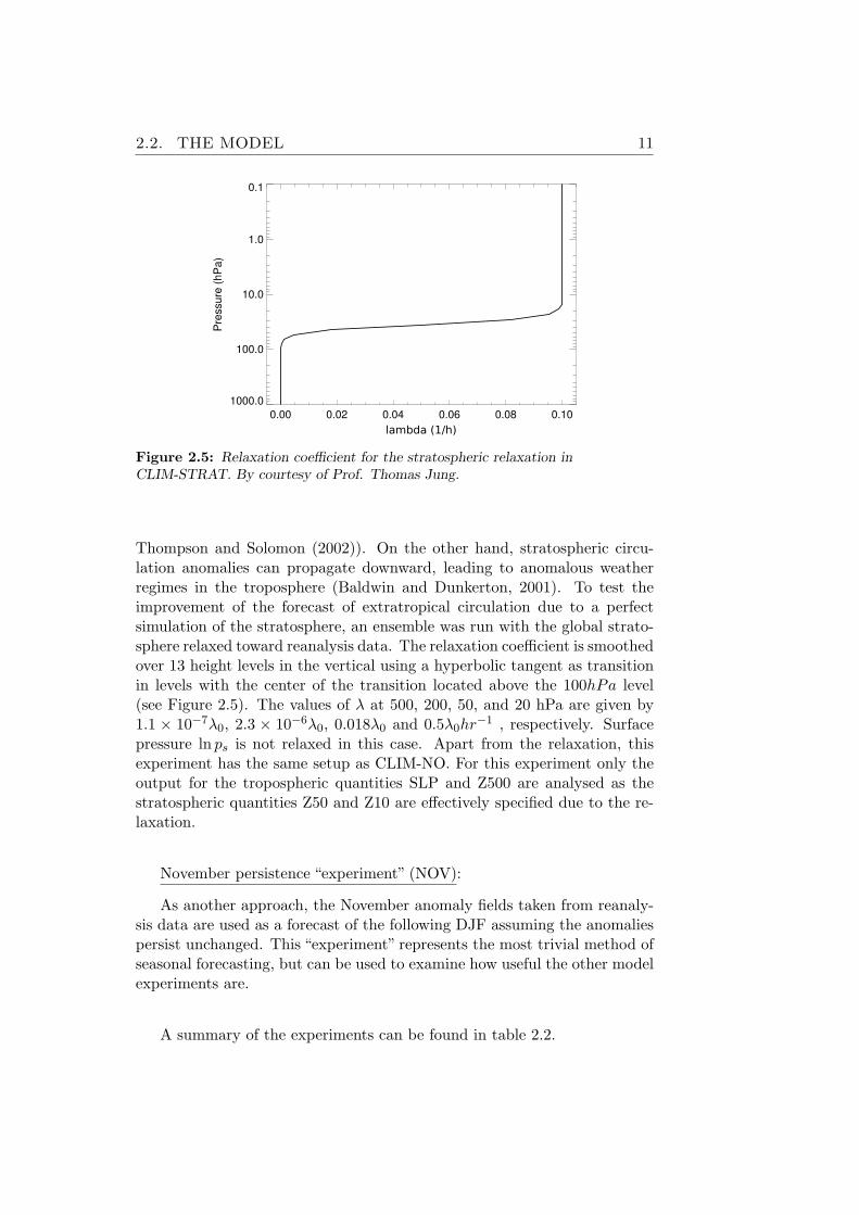
Figure 2.5: Relaxation coefficient for the stratospheric relaxation inCLIM-STRAT. By courtesy of Prof. Thomas Jung.
Thompson and Solomon (2002)). On the other hand, stratospheric circu-lation anomalies can propagate downward, leading to anomalous weatherregimes in the troposphere (Baldwin and Dunkerton, 2001). To test theimprovement of the forecast of extratropical circulation due to a perfectsimulation of the stratosphere, an ensemble was run with the global strato-sphere relaxed toward reanalysis data. The relaxation coefficient is smoothedover 13 height levels in the vertical using a hyperbolic tangent as transitionin levels with the center of the transition located above the 100hPa level(see Figure 2.5). The values of λ at 500, 200, 50, and 20 hPa are given by1.1 × 10−7λ0, 2.3 × 10⁻⁶λ0, 0.018λ0 and 0.5λ0hr
−1 , respectively. Surfacepressure ln ps is not relaxed in this case. Apart from the relaxation, thisexperiment has the same setup as CLIM-NO. For this experiment only theoutput for the tropospheric quantities SLP and Z500 are analysed as thestratospheric quantities Z50 and Z10 are effectively specified due to the re-laxation.
November persistence “experiment” (NOV):
As another approach, the November anomaly fields taken from reanaly-sis data are used as a forecast of the following DJF assuming the anomaliespersist unchanged. This “experiment” represents the most trivial method ofseasonal forecasting, but can be used to examine how useful the other modelexperiments are.
A summary of the experiments can be found in table 2.2.

12 CHAPTER 2. DATA AND MODEL
Table 2.2: Short description of the experiments
Abbreviation model run SST + sea ice relaxation
CLIM-NO X climatological noneOBS-NO X observed noneCLIM-TROP20 X climatological tropical, 20N-20SCLIM-TROP10 X climatological tropical, 10N-10SOBS-TROP20 X observed tropical, 20N-20SCLIM-STRAT X climatological stratosphereNOV × Nov anomaly persistence
2.3 NAO and NAM - North Atlantic Oscillationand Northern Annular Mode
The NAO is the leading mode of variability in the North Atlantic Sector(NAS) and is therefore used in this thesis to investigate the variability inthis sector (Greatbatch, 2000; Hurrell et al., 2003). It corresponds to fluctu-ations in the mid-latitude jet stream, the meridional displacement of stormtracks, the number of storms generated and the distribution of precipitationand temperature anomalies around the North Atlantic basin. The NAO pat-tern for SLP in boreal winter can be found in Figure 2.7. It represents theintensity of the typical Icelandic low and the Azores high pressure systems(at sea level), which are most pronounced in Boreal winter (DJF). Changesin the NAO can have a great impact on the densely populated areas of West-ern Europe, so that a lot of studies were done to investigate the variability ofthe NAO at all timescales (Hurrell, 1995; Semenov et al., 2008; Jung et al.,2011).There are a lot of different ways to measure the state of the NAO. One ofthe oldest definitions is the normalised SLP difference between station mea-surements at or near the centers of action of the NAO, which are the Azores,Lisbon or Gibraltar for the center of high pressure and Iceland for center ofthe low pressure system, as defined by Hurrell (1995). This approach has theadvantage of providing long time series, which can be derived back to theearly 1820s due to long station records (Jones et al., 1997), but some featuresof the circulation pattern associated to the NAO do depend on the choice ofthe stations as there are several possibilities especially for the choice of thesouthern station. A more sophisticated measure of the NAO is the princi-pal component of an Empirical Orthogonal Function (EOF)/Singular ValueDecomposition (SVD) analysis of gridded SLP or Z500 anomaly data withinthe NAS, defined as the region bounded by 20◦N − 80◦N , 90◦W − 40◦E(as defined by Hurrell, 1995). The large scale characteristics can then befound, for example the displacement of the centers of action over seasonsand decades (Barnston and Livezey, 1987; Hurrell et al., 2003), but also

2.3. NAO AND NAM 13
displacement between different NAO regimes (Peterson et al., 2003; Hilmerand Jung, 2000). The NAO can be defined by using geopotential heights ofdifferent pressure levels or by using sea level pressure fields.
In this thesis we will use geopotential heights of the 500hPa level and theregion bounded by 30◦N−80◦N , 90◦W −40◦E as the region to calculate theNAO. We change the southern boundary to 30oN to avoid ambiguousnessassociated to the intersection of the analysis region and the region where re-laxation was applied in the case of the tropical relaxation in CLIM-TROP20and OBS-TROP20. The index corresponding to this definition (see Figure2.6) is very strongly correlated to the standard NAO index
The NAM index expresses the extratropical variability throughout thewhole northern hemisphere, so it has originally been defined as the principalcomponent in SLP or geopotential height anomalies north of 20◦N at alllongitudes by Thompson and Wallace (1998). In the troposphere it is alsoreferred to as the Arctic Oscillation (AO) index of which the correspondingpattern has separated centers of action of high pressure at mid latitudesand low pressure extending over the pole at high latitudes respectively. TheNAM is more commonly used in the stratosphere, where the NAM index isa measure for the polar vortex and the patterns have a more annular shape.In the stratosphere, the annular mode is only present during winter, becauseduring summer easterlies dominate in the NH extratropics due to the solarradiation which warms the polar stratosphere. For this thesis we define theNAM as the first PC north of 30oN for the same reason as for the NAO(relaxation boundaries in the case of CLIM-TROP20 and OBS-TROP20)which is shown in Figure 2.6.
In Figure 2.6 some examples of different winter NAO and NAM indicesare given, while in Figure 2.7 the regression pattern for the Principal Com-ponent (PC) - based NAO index in SLP (index (a) in Figure 2.6) and inZ500 (index (d)) can be found for the NAS north of 30oN (see Chapter 3for methods). On the one hand the robustness of the index in differentmethods, datasets and height levels can be seen as the indices all have astrong correlation. Only the NAM index for the stratosphere shows someindependent variability in some years or periods, for example in the mid1960s or the late 1990s, and is therefore less well correlated to the NAOindex in SLP. On the other hand from the 1970s to the mid 1990s a trendto a more positive state can be seen, consistent with the findings by, e.g.,Hurrell (1995); Thompson et al. (2000).
The NAO reveals a more or less white power spectrum. This does not ex-clude the possibility of having some decades with pronounced low frequencyvariability as noted by Wunsch (1999). For example we can find three con-secutive low NAO winters during the late 1970s and five high NAO wintersduring the early 90s. These phases of “persistence” do not need to have anycause but can be produced by the chance of white noise.
In Figure 2.7 (top) the SLP NAO anomaly pattern shows the impact of a

14 CHAPTER 2. DATA AND MODEL
1965 1970 1975 1980 1985 1990 1995 2000−4
−2
0
2
Comparison of NH climate indices, each index normalized by its STD
(a) (b) (c) (d) (e) (f)
Figure 2.6: NAO and NAM indices for the Northern Hemisphere (NH)calculated from ERA-40 reanalysis data except (c), which is Hurrell’s indexcalculated from the NCEP/NCAR reanalysis dataset (downloaded fromhttp://www.cgd.ucar.edu/cas/jhurrell/indices.data.html#naopcdjf).(a) NAO: first PC for SLP anomalies in Hurrell’s sector: 20◦N − 80◦N ,90◦W − 40◦E;(b) NAO: normalised SLP difference between the Azores (37.5◦N, 27.5◦W ) andIceland (65◦N, 22.5◦W );(c) NAO: same as (a) but for NCEP/NCAR reanalysis data;(d) NAO: first PC for 500hPa height anomalies in the NAS: 30◦N − 80◦N ,90◦W − 40◦E, (used in this study);(e) NAM: as (d) but for the whole NH north of 30oN;(f) NAM: as (e), but for 50hPa height anomalies (lower stratosphere).
positive NAO index of +1 standard deviation, corresponding to index (a) inFigure 2.6. This index is the first PC of an EOF analysis of SLP data in thesector 20oN - 80oN and 90oW - 40oE. The negative anomaly correspondingto the Icelandic low has a minimum of 5hPa while the positive anomaly ofthe Azores high has a maximum of 4hPa. In comparison with the Icelandiclow and the Azores high in the SLP climatology in Figure 2.2 we can seethat the centers of action of the NAO pattern are displaced northward. Ad-ditionally the negative anomaly corresponding to the Icelandic low extendsmore into the south in its eastern tail over the Eurasian continent. Dueto geostrophy, the isobars can nearly be seen as the streamfunctions of theanomaly flow field, implying enhanced westerlies during high NAO phasesin north-western Europe and western Russia. In Figure 2.7 (bottom) theregression pattern corresponding to index (d) (used in this study) for the500hPa level is shown, obtained within the same sector as the SLP NAOpattern but with the southern boundary shifted from 20oN to 30oN . So,it can be seen that the patterns are very similar, only with the northerncenter of action shifted slightly westward at Z500 and extending further tothe Pacific side of the pole than at mean sea level.

2.3. NAO AND NAM 15
120
o W
60 oW
0o
60
o E
120 oE
180oW
30oN
45oN
60oN
75oN
mslp, NAO−pattern, exvar = 0.48631, c−int = 0.5 hPa
120
o W
60 oW
0o
60
o E
120 oE
180oW
30oN
45oN
60oN
75oN
z500, NAO−pattern, exvar = 0.43835, c−int = 10 m
Figure 2.7: NAO patterns for SLP (top) and Z500 (bottom). The pattern forSLP (Z500) is obtained by the regression of mean DJF SLP (Z500) anomaliesfrom ERA-40 between 1960/61 and 2001/02 onto the observed NAO time series(a) shown in Fig. 2.6 (index (d) for Z500). The variance explained by this patternwithin the Atlantic sector in winter is 48.6% (43.8%). Note that the patterns aresimilar, although referring to different heights and are based on different sectorsfor the calculation (20oN - 80oN for SLP and 30oN - 80oN for Z500, 90oW -40oE for both heights). Contour interval is 0.5 hPa (10m).

16 CHAPTER 2. DATA AND MODEL
2.4 PNA - Pacific North America pattern
The PNA index is the counterpart of the NAO in the extratropical Pacificand basically measures the strength of the Aleutian low. It is the modeof variability in the North Pacific which corresponds to the distribution ofSLP, surface air temperature (SAT) and precipitation anomalies around theNorth Pacific basin as well as to SST and sea ice (SSTSI) anomalies andmixed layer depths in the North Pacific. It is closely connected to otherNorth Pacific indices, such as the North Pacific Index (NPI) or the Paci-fic Decadal Oscillation (PDO) (SST index), c.f. Mantua et al. (1997). Asan indicator of interannual variability in the troposphere with focus on theNorth Pacific, we choose the PNA index here to examine the skill of therelaxation experiments in this sector.
The PNA index was originally defined as a four point index of 500hPaheight anomalies, including the Aleutian low and the corresponding ridgeover Canada (see Wallace and Gutzler (1981)). The PNA index has beenrevised to several versions, such as a weighted area mean of SLP over theNorth Pacific sector (160◦E− 140◦W and 30◦N − 65◦N , NPS, suggested byTrenberth and Hurrell (1994)). This index is used in this study and also theminus of the weighted area mean of 500hPa height anomalies over the samesector.
In modelling studies and also in observations it was found that the Aleu-tian low is deeper (positive PNA index) during a warm ENSO event (Tren-berth and Caron, 2000; Alexander et al., 2002). This is caused by the ex-citation of Rossby waves due to anomalies in equatorial convection whichtransport momentum to the mid-latitudes, enhancing westerlies in the lati-tude band 20◦−40◦ in both the North and South Pacific. These extratropicalatmospheric anomalies can in turn influence surface heat fluxes and thereforeSSTs in the North Pacific. The remote connection between tropical SSTsand extratropical SSTs has been called an “atmospheric bridge” (Alexanderet al., 2002).
It was found that North Pacific climate underwent a shift around thelate 1970s towards a deeper Aleutian low and therefore a higher PNA in-dex. This caused for example lower surface temperatures (and SSTs) in thecentral North Pacific, higher temperatures in the Alaskan region resultingin warmer SSTs and diminishing Salmon stocks thereafter (Trenberth andHurrell, 1994; Mantua et al., 1997). A number of remote teleconnections as-sociated to the Pacific such as the connection between ENSO and Europeanwinter climate show a regime shift from the period before the late 1970s andafterwards (Greatbatch et al., 2004).
In Figure 2.8 five different Pacific indices can be found. Indices (a),(b),(c) and (d) indicate North Pacific atmospheric variability, derived fromERA-40 reanalysis data and show high correlation between different methods

2.4. PNA 17
1965 1970 1975 1980 1985 1990 1995 2000−4
−2
0
2
North Pacific indices, each index normalized by its STD
ST
D
(a) (b) (c) (d) (e)
Figure 2.8: Normalised North Pacific climate indices, all from ERA-40:(a) negative of PNA index, the weighted area mean of 500hPa anomalies over theNorth Pacific sector: 30◦N − 65◦N , 160◦E − 140◦W defined by Trenberth andHurrell (1994);(b) negative of NPI index which is the weighted area mean of SLP anomalies overthe same sector as for (a);(c) PNA 4-point index defined by Wallace and Gutzler (1981) as: PNA =14 [z
∗(20◦N, 160◦W )− z∗(45◦N, 165◦W ) + z∗(55◦N, 115◦W )− z∗(30◦N, 85◦W )]with z∗ being the 500hPa height anomalies normalised by their standarddeviation;(d) first PC of an EOF analysis of 500hPa anomalies over the same sector as for(a);(e) Nino 3.4 SST index, data from NCAR (original time series (1871-2007): http://www.cgd.ucar.edu/cas/catalog/climind/TNI_N34/index.html#Sec5)and normalised by its standard deviation for winters from 1961-2002.
and heights in the troposphere. Index (e) is the El Nino 3.4 index suggestedby Trenberth (1997), which is defined as the 5-month running means ofSST averaged over the area (120◦W − 170◦W, 5◦S − 5◦N) and calculatedfrom NCEP/NCAR SST data (data from http://www.cgd.ucar.edu/cas/
catalog/climind/TNI_N34/index.html#Sec5). It is interesting to see thatthe correlation between the Nino 3.4 and the PNA index is low in the firsthalf of the entire period (i.e., 0.26) and high in the second half (0.60). Thechange in correlation is probably connected to the climate shift in the late1970s changing the impact of tropical SSTs on the extratropical atmosphericcirculation in the Pacific sector. This shift can also be seen in Figure 2.8.Before 1977, only two winters of a positive PNAm index were found, whereasin the following twelve years nine winters of a positive and only three of anegative PNA index were found, the positive PNA winters being much morepronounced thereby. After 1988 the PNA went to a more balanced phasewith only two winters which exceeded one standard deviation in the PNAindex.
In Figure 2.9 the regression pattern of index (a) can be found, showingthe positive phase, corresponding to +1 standard deviation, of the PNApattern in 500hPa with the trough over the North Pacific associated to theAleutian low and a ridge over Canada.

18 CHAPTER 2. DATA AND MODEL
120
o W
60 oW
0o
60
o E
120 oE
180oW
30oN
45oN
60oN
75oN
z500 PNA−pattern, contour = 10 m
Figure 2.9: PNA pattern obtained by regression of observed (ERA-40, 1960/61to 2001/02) DJF 500hPa height anomalies onto the observed PNA time series (a)shown in Fig. 2.8. The variance explained by this pattern within the NorthPacific sector in winter is 53.5%. Contour interval is 10m.

Chapter 3
Methods
3.1 Linear regression and correlation
If x and y are continuous random variables of length T , the evolution of ycan be estimated in a linear-least-square sense if x is assumed to be knownwith precision:
y = a0 + a1 · x+ ε (3.1)
with some uncertainty, expressed by the error ε. Then the linear regressioncoefficient a1 which estimates the dependence of y on the regressor x is
a1 =x′y′
x′2, (3.2)
where x′ = x−x are anomalies deviating from the arithmetic mean x. Hereand in the following all notations defined for x are also valid for y. Thecovariance of x and y is defined by:
Covxy = x′y′ =1
T − 1
T∑t=1
x′y′ (3.3)
Another measure of the relationship between x and y is the correlationρxy, which assumes uncertainties for both variables:
ρxy =x′y′
σxσy,−1 ≤ ρ ≤ 1 (3.4)
where σx is the standard deviation (STD) of x, the square-root of the vari-ance of x, V ar(x):
σx =√
V ar(x) =
√√√√ 1
T − 1
T∑t=1
(x′)2 (3.5)
ρ2xy is the fraction of explained variance of y explained by x in a linearleast-square sense and vice-versa.
19
20 CHAPTER 3. METHODS
3.2 Weighting and projection
When working with geographical maps on a sphere, one often has to con-sider the latitudinal dependence of the size of the grid boxes. Otherwisein projections or covariances, the gridboxes near to the poles are given toomuch weight as the number of gridboxes increases towards the poles onmany types of grids. The results of any analysis should be independent ofthe choice of the grid type. For a regular longitude-latitude grid, weightingis done by multiplying the value at each grid point with the cosine of itscorresponding latitude θ. To explain the method in matrix notations, anarea-weighting matrix can be defined as a diagonal matrix with the samesize as the covariance matrix of the data. In the case of a data set X storedon a regular longitude-latitude grid with m longitudes and n latitudes fromT observational time steps
X ε Rm×n×T .
There are S = m · n grid points so that the spatial dimensions of X can bemerged to one dimension:
X ε RS×T
Then the weighting matrix is (see Baldwin et al. (2009))
W ε RS×S , Wij = cos(θ)δij (3.6)
with the Kronecker delta defined as
i = j ⇒ δij = 1
i 6= j ⇒ δij = 0 .
This is in fact the weighting matrix we will use throughout the presentstudy. For example before computing the variance of X the data has to bemultiplied with the square-roots of cos(θ), expressed here as the weightingmatrix W 1/2:
Xw = W 1/2 ·X (3.7)
var(X) =1
T − 1
(X ′
w ·X ′w
t)
(3.8)
Xt denotes the transpose matrix of a matrix X. If X is the time average ofX, X ′ = X −X is the anomaly field.
Projections examine the linear dependence of one vector or field on an-other one. If X and Y are fields of the same length S, this is done bycalculating the scalar product of the weighted fields:
〈Xw | Yw〉 =S∑
i=1
Xw,iYw,i ε R (3.9)

3.3. EOF ANALYSIS 21
With other grid types, such as Gaussian grids, the weighting matrix W con-tains values other than cos(θ) and its elements can be taken from referencetables.
3.3 Empirical orthogonal functions (EOF)
The EOF analysis is a method to decompose any data set into linearly in-dependent modes. In climate dynamics EOFs can be used to derive theoriesfor mechanisms or to extract reoccuring and therefore possibly predictablephenomena. Other applications also make use of the EOFs, e.g., the jpg for-mat for images uses a limited number of EOF modes of an image to presentthe image using a smaller data set. A detailed description of the EOF prob-lem and derivation of the connections explained below can be found in vonStorch and Zwiers (2001).
Let D be a climate data set with m longitudes, n latitudes and T obser-vations.
D ε Rm×n×T .
The EOFs are based on the covariance matrix of the field, so the spatialdimensions have to be merged to obtain a two dimensional matrix for D:
D ε RS×T
with S = m · n. Additionally, as explained in Section 3.2, the field has tobe weighted with W 1/2 when considering variances and the temporal meanhas to be removed so that the elements of the covariance matrix of D are
cov(D)ij =1
T − 1
T∑t=1
D′it,wD
′jt,w. (3.10)
cov(D) is symmetric and has the dimensions cov(D) ε RS×S . The EOFs arethen the eigenvectors ~ei of the covariance matrix of D which have unit length(Euclidean norm) and together with the eigenvalues λi solve the eigenvalueproblem
(cov(D)− λiIS) ~ei = 0 (3.11)
where IS is the identity matrix with the size of cov(D). There are S eigenvec-tors which can be written as the rows of a matrix E and the correspondingeigenvalues can be written as one vector ~λ:
E ε RS×S (3.12)
~λ ε RS . (3.13)
There are S eigenvalues of which r are non-zero and it can be shown that
r = rank(cov(D)) =S · TS + T
(3.14)

22 CHAPTER 3. METHODS
which means that if one of S or T is much larger than the other, r will con-verge towards the smaller one. In our case 42 winter means define the timedimension and a much larger amount of grid points (O(10000)) is given, itfollows from (3.14) that r ≈ T = 42. The corresponding principle component(PC) time series can be obtained by projecting (see Section 3.2) the weightedanomaly fields Dw onto the EOF patterns (which are already weighted) forevery timestep which can be expressed by the matrix multiplication:
PC = E ·Dw . (3.15)
The PC time series are then given as a matrix which has S rows and Tcolumns:
PC ε RS×T
The dataset D at any timestep t can then be reconstructed by the linearcombination of the EOF modes:
Dt =
S∑i=1
PCit ~ei (3.16)
From the definition it follows that the modes are characterised by the or-thogonality of the spatial patterns, i.e.
〈~ei|~ej〉 = 0 ∀ i 6= j (3.17)
and that their time series are uncorrelated, i.e.
ρPCiPCj = 0 ∀ i 6= j (3.18)
The variance of D is the sum of the eigenvalues of the covariance matrix,while each eigenvalue λi is the variance explained by the corresponding eigen-mode:
var(D) =
S∑i=1
λi ⇒ explained variance[%] =λi
V ar(D)(3.19)
For the presentation of the EOFs the spatial patterns ~ei, which have unitlength, are multiplied by the standard deviation of each mode σi =
√λi to
obtain the patterns in the same dimensions as the data itself, whereas thetime series are normalised by their standard deviation:
~ei∗ =
√λi~ei (3.20)
PC∗i =
1√λi
PCi (3.21)
The sign of an EOF pattern is thereby arbitrary and can be changedsimultaneously with that of its PC time series to consider its climatological

3.4. PATTERN CORRELATION 23
relevance. It is important to note that the results of an EOF analysis haveto be interpreted with caution since the constraint of orthogonality in spacecan lead to spurious results especially in the higher order EOFs. These donot have to be consistent with the natural modes of variability (Dommengetand Latif, 2002). However, the EOF modes presented in this study and usedfor the analysis have a maximum order of two and have been proved to agreewith the results from different methods as described in Sections 2.3 and 2.4.They can therefore be interpreted as “real” physical modes.
3.4 Pattern correlation
To compare the spatial structure of two patterns regarding their linear de-pendence without considering the amplitude, one can calculate the patterncorrelation. The weighted area mean of each of the patterns X,Y ε RS hasto be subtracted:
X = X −
(∑Si=1 cos(θi)Xi∑Si=1 cos(θi)
)(3.22)
It is important again that the patterns are weighted before computing thecorrelation (see Section 3.2). In this case the weighting is done with W 1/2:
Xw = W 1/2X (3.23)
The correlation is then calculated as defined in Section 3.1:
ρpatt(X,Y ) =
∑Si=1
ˆXw,iˆYw,i
σXwσYw
; (3.24)
An illustration of pattern correlation can be found in Figure 3.1.

24 CHAPTER 3. METHODS
120
o W
60 oW
0o 6
0o E
120 oE
180oW
30oN
45oN
60oN
75oN
1962/1963, ERA−40, c−int=2
120
o W
60 oW
0o
60
o E
120 oE
180oW
30oN
45oN
60oN
75oN
CLIM−TROP, ρpc
=0.66 CLIM−NO, ρpc
=−0.51
120
o W
60 oW
0o
60
o E
120 oE
180oW
30oN
45oN
60oN
75oN
1962/1963, ERA−40 − norm, c−int=0.5
120
o W
60 oW
0o
60
o E
120 oE
180oW
30oN
45oN
60oN
75oN
CLIM−TROP,ρpc
=0.66 1
20o W
60 oW
0o
60
o E
120 oE
180oW
30oN
45oN
60oN
75oN
CLIM−NO, ρpc
=−0.51
120
o W
60 oW
0o
60
o E
120 oE
180oW
30oN
45oN
60oN
75oN
Figure 3.1: SLP anomalies in the NH for winter 1962/1963, first row showingthe observed anomalies and ensemble means (CLIM-TROP20 and CLIM-NO) andsecond row showing the anomalies for which the area mean of each pattern hasbeen subtracted as described in Section 3.4, equation (3.22). Furthermore, eachpattern is normalized by its weighted standard deviation to show only thosefeatures of the pattern which are relevant for ρpatt. ρpatt between the ensemblemean and reanalysis data is given in the figure. Contour interval in the first row is2hPa and 0.5 in the second row.
3.5 Monte Carlo methods
To test the significance of statistical parameters like trends and correlationsof continuous random variables, Monte Carlo methods are applied. Thismethod can be used as an alternative to the Student’s t-test and is called“Monte Carlo”, referring to the games of chance commonly played in MonteCarlo, Monaco, and was first described by Metropolis and Ulam (1949). TheMonte Carlo method is based on the assumption that the average of the re-sults comes closer to the theoretically expected value the larger the numberof trials that are used (the law of large numbers; Hsu and Robbins (1947)).In the following we use the NAO index as an example. This method involvesgenerating time series of the NAO index from the model results with whichto compare the observed time series. The Monte Carlo method is best illus-trated by examples.

3.5. MONTE CARLO METHODS 25
Case 1: Is the correlation between the ensemble mean NAO index from a par-ticular model experiment and the observed NAO index significantlydifferent from zero?
• 12 artificial time series of the NAO index are produced by ran-domly selecting (without replacement) 42 values 12 times fromthe original 12 × 42 = 504 values available from the model re-sults. The ensemble mean NAO index is then calculated fromthe selected values for each year and the correlation between thetimes series of this ensemble mean index and the observed NAO iscomputed. The process is then repeated a large (typically 10,000)number of times and a histogram of the ensemble mean values iscomputed to produce the probability distribution function (PDF)of the correlation values. All histograms have 50 bins and are nor-malized to have an integral of 1.
• The resulting PDF is centered around zero and significance levelscan be derived by calculating the correlation ranges correspondingto percentiles, e.g., the 5% or 95% percentiles. The significanceof the correlation between the actual ensemble mean NAO indexfrom the model experiment and the observed index can then beassessed by noting into which percentile it falls.
• The results agree with Student’s t-test if 42 degrees of freedomare assumed. Serial correlation (memory from one winter to thenext) would reduce the number of degrees of freedom and increasethe threshold correlations for significance. Although not thoughtto be a serious problem for the NAO and the PNA, this possibilityshould be kept in mind when interpreting the results.
Case 2: How unusual is the observed NAO trend in the context of an particularmodel experiment?
• A large number (e.g., 10000) of time series of the NAO index areproduced by picking one value for the NAO index from the 12original members for each year, keeping the order of the yearsas in the original experiment. Noting that the real world corre-sponds to a single realization, it is clear that any of the selectedrealisations could correspond to the observed NAO time serieswithin the context of the particular model experiment. The trendis then computed for each realization and a PDF of trends is pro-duced as described above for the correlation values.
• The PDFs of all cases will, to a good approximation, be centeredaround the trend of the original ensemble mean NAO index from

26 CHAPTER 3. METHODS
the experiment and it can then be seen into which percentile ofthe PDF the observed trend falls.
Case 3: Which correlations between the time series of the NAO index of singlerealisations and the observed NAO index are possible? How strong isthe added forcing in each experiment?
• Possible realisations are produced as for the trends above and thecorrelation between the NAO index of the new realisations andthe observed NAO index is calculated to produce a PDF of thesecorrelations.
• The resulting PDF is centered around a correlation value whichis lower than the correlation of the ensemble mean NAO indexwith the observed one (see Bretherton and Battisti (2000)).
• Depending on how much the resulting PDF is shifted away fromzero one can conclude how strong the added forcing is. Likewise,these PDFs give an indication of how realistic the model simu-lations are compared to the observations. The more the PDF isshifted towards positive correlations, the more realistic the corre-sponding model setup represents the variability of the real worldin our period.
In all cases, the shuffling is carried out by randomly selecting numbers froma uniform distribution of integers between 1 and 12 or 1 and 42 respectively.

Chapter 4
Results
The results of our model experiments will be presented by means of com-parison with the reanalysis data set ERA-40 (hereafter referred to as theobservations). There are separate sections for the analysis of interannualvariability as a measure of the seasonal forecasting skill of the different ex-periments (Section 4.1), and the investigation of trends during winters from1961 to 2002 (Section 4.2). First of all it is useful to say that our model(an AGCM, see Section 2.2) reveals similar modes of variability comparedto the observations if, for example, an EOF analysis is carried out as for theobservations. See Figures 2.4 and 2.7 for comparison of the NAO patternsobtained from the “control” experiment CLIM-NO and the observations.The model therefore represents well the internal variability of the real atmo-sphere and it is consistent to produce NAO/PNA indices for the experimentsby projecting the model anomaly fields onto the spatial patterns which re-sult from the analysis of the observational data (see Chapters 2 and 3 fordetails).
As a measure of the model’s skill to produce a seasonal forecast, patterncorrelations between fields from observations and ensemble member fieldsare used in Section 4.1. The correlations between the observed NAO (PNA)index and the model NAO (PNA) indices are discussed in Sections 4.1.1 and4.1.2. The correlation measure does not consider the variance of each timeseries, but it is a measure of the tendency of both indices to vary coherentlyand of the constancy of the ratio of their magnitudes. The correlation overthe whole period is a measure of the capability of the model to forecast thewinter mean value of the given index. In Figure 4.1 a schematic summaryof the results of the correlation analysis corresponding to ensemble meanscan be found for the 500hPa geopotential heights.
In Section 4.2 trends are investigated in terms of their patterns and alsotheir amplitude. Figure 4.2 gives a summary of the results of the trendanalysis in terms of the amplitude of the NAO and PNA trend which isrepresented by the different experiments.
27

28 CHAPTER 4. RESULTS
−1 −0.8 −0.6 −0.4 −0.2 0 0.2 0.4 0.6 0.8 1
CLIM−STRAT
OBS−TROP20
CLIM−TROP20
OBS−NO
NOV
CLIM−NO
correlation (ERA−40,ensemble mean)
correlation not significantly different from zeroNAO correlationPNA correlation
Figure 4.1: Schematic summary of the correlations between the observedNAO/PNA index and the NAO/PNA index of the ensemble means at 500hPa.NAO index (black circles) and PNA index (red circles). A description of theexperiments can be found in Section 2.2.1. Correlations lower than 0.31 are notsignificantly different from zero, as they lie within the 95% confidence intervalaccording the results of the Monte Carlo simulations explained in Section 3.5. InSections 4.1.1 and 4.1.2 it is found that the significance levels do not differsubstantially between the experiments and for either the NAO or PNA index.
−1 −0.5 0 0.5 1
CLIM−STRAT
OBS−TROP20
CLIM−TROP20
OBS−NO
NOV
CLIM−NO
trend ratio: ensemble mean/ERA−40
NAO trend ratioPNA trend ratio
Figure 4.2: Schematic summary of the analysis of the trends of the NAO andPNA indices at 500hPa. NAO index (black crosses) and PNA index (red crosses).The ratio of each ensemble mean trend with the observed trend is shown, so thecloser the ratio is to 1, the better the representation of the trend in thecorresponding experiment. A description of the experiments can be found inSection 2.2.1 and especially Table 2.2.

4.1. SEASONAL FORECASTING 29
4.1 Seasonal forecasting
In Figures 4.3 and 4.4 the pattern correlations ρpc of Z500 anomalies of en-semble members with the observed anomalies from the corresponding yearsare summarised as histograms. The histograms of all 42 winters and all12 ensemble members are shown to examine which spatial correlations oc-cur most frequently for the selected experiments and the sectors of interest.However, for the persistence “experiment”NOV only 42 values are available.The pattern correlation shows the skill of the model to forecast the meanwinter circulation and shows which forcing has the largest effect. The av-erage of the pattern correlations at 500hPa for all years for all ensemblemembers for the NH (≥ 30oN), the NAS (30◦N − 80◦N , 90◦W − 40◦E) andthe North Pacific Sector (NPS) (30◦N−65◦N , 160◦E−140◦W ) are shown inTable 4.1. In Table 4.2 the fraction, i.e., the probability of positive patterncorrelations for the whole set of realisations of each experiment is noted.
In the Northern Hemisphere (NH), the values for CLIM-NO and NOVresemble a normal Gaussian distribution with mean zero (Fig. 4.3, Table4.1) The results are very similar in the NAS and the NPS (only shown inthe tables). The fraction of positive ρpc is around 50% for the ensemblemembers of both experiments, which indicates that there is no forecast skillusing these methods.
For the experiments with tropical relaxation, the ensemble members gen-erally yield higher pattern correlations compared to the other cases and thehighest values occur with tropical relaxation in OBS-TROP20 in all sectors,especially in the NPS where the spatial correlation is ρpc = 0.45 in the av-erage. However, it is noticeable that for CLIM-TROP20, where SSTs are ina climatological cycle, the pattern correlations of the single realisations areof a similar magnitude as those of OBS-TROP20 (ρpc = 0.40 in the averagein the NPS) and it can be concluded that the origin of the high correlationis located in the tropics rather than in the prescribed extratropical SSTand sea ice (SSTSI). For the tropical relaxation experiments, 80 − 90% ofthe realisations yield positive pattern correlations if the NH and the NPSare considered. In the NAS only 60 − 70% of ρpc are positive, indicatingthat the tropical forcing is still not enough to represent the variability, butnevertheless has a clear impact compared to CLIM-NO and NOV.
In Figures 4.3 and 4.4 the results for CLIM-STRAT realisations are alsoshown. Stratospheric relaxation has little influence in the NPS as the pat-tern correlations are nearly equally distributed with some kurtosis so thatlarge positive and negative ρpc are likely, suggesting a bimodal response tothe stratosphere . For the NH and NAS, CLIM-STRAT slightly shifts thecorrelations to positive values and with a normal-like distribution (see Figure4.4 and Table 4.1). Slightly more than 50% of ρpc are positive (Table 4.2). Inthe NAS both CLIM-TROP20 and CLIM-STRAT have their mean shiftedto positive values while CLIM-TROP20 is in the average higher (ρpc = 0.15)

30 CHAPTER 4. RESULTS
−1 −0.8 −0.6 −0.4 −0.2 0 0.2 0.4 0.6 0.8 10
10
20
30
40
50z500, NH
CLIM−NO
case
s
−1 −0.8 −0.6 −0.4 −0.2 0 0.2 0.4 0.6 0.8 10
2
4
6
8
10
NOV
ρpc
case
s
−1 −0.8 −0.6 −0.4 −0.2 0 0.2 0.4 0.6 0.8 10
10
20
30
40
50z500, NH
CLIM−STRAT
case
s
−1 −0.8 −0.6 −0.4 −0.2 0 0.2 0.4 0.6 0.8 10
10
20
30
40
50
CLIM−TROP20
ρpc
case
s
Figure 4.3: The histograms of pattern correlations between observations andNovember anomalies for all 42 winters (NOV) and between observations and allensemble members (others), all within the extratropical northern hemisphere (NH,≥ 30oN). In the upper two panels the pattern correlations with CLIM-NO (1st)and NOV (2nd) are shown for comparison, showing a normal-like distributionwith the mean near zero. The lower two panels are the pattern correlations for thetwo relaxation experiments CLIM-STRAT (3rd) with the mean slightly shifted topositive correlations and CLIM-TROP20 (4th) with the clearest improvement.The average pattern correlations of the ensemble members for all experiments aregiven in Table 4.1.

4.1. SEASONAL FORECASTING 31
−1 −0.5 0 0.5 10
50z500, NAS
OBS−NO
case
s
−1 −0.5 0 0.5 10
50OBS−NO
z500, NPS
−1 −0.5 0 0.5 10
50CLIM−TROP20
case
s
−1 −0.5 0 0.5 10
50CLIM−TROP20
−1 −0.5 0 0.5 10
50OBS−TROP20
case
s
−1 −0.5 0 0.5 10
50OBS−TROP20
−1 −0.5 0 0.5 10
50CLIM−STRAT
r
case
s
−1 −0.5 0 0.5 10
50CLIM−STRAT
r
Figure 4.4: Pattern correlation histograms for the North Atlantic sector (NAS,30◦N − 80◦N and 90◦W − 40◦E, left column), the North Pacific sector (NPS,30◦N − 65◦N and 160◦E − 140◦W , right column) and for the experimentsOBS-NO (1st row), CLIM-TROP20 (2nd row), OBS-TROP20 (3rd row) andCLIM-STRAT (4th row). The mean pattern correlations for all experiments aregiven in Table 4.1. A strong impact of the tropical relaxation can be seen for theNPS, while in the NAS the impact of tropical and stratospheric relaxation are lessobvious, but still visible.

32 CHAPTER 4. RESULTS
Table 4.1: Average pattern correlations ρpc between single model realisations(single years for NOV) and observations at Z500. Values are given for theextratropical northern hemisphere (NH), the North Atlantic sector (NAS) and theNorth Pacific sector (NPS). The values noted here are also the means of thecorresponding distributions shown in Figures 4.3 and 4.4.
Experiment NH NAS NPS
CLIM-NO -0.01 -0.04 -0.02NOV 0.02 < 0.01 0.03OBS-NO 0.11 0.08 0.18CLIM-TROP20 0.24 0.15 0.40OBS-TROP20 0.29 0.20 0.45CLIM-STRAT 0.06 0.08 0.01
Table 4.2: The probability of positive pattern correlations between all singleensemble members from each experiment for all years in percent (100%correspond to 504). The pattern correlations are computed for 500hPa heightanomalies as for Figures 4.3 and 4.4. The number of positive correlations for themodel experiments is therefore divided by 12× 42 = 504 and by 42 for the NOVexperiment.
Experiment NH NAS NPS
CLIM-NO 49 46 48NOV 52 48 50OBS-NO 66 60 65CLIM-TROP20 83 63 84OBS-TROP20 86 67 86CLIM-STRAT 56 58 51
correlated to the observations than CLIM-STRAT (ρpc = 0.08).
Globally prescribed observed SSTSI in OBS-NO lead to slightly higherpattern correlations in the NH, and especially the NPS, where the averagespatial correlation between ensemble members and observations is ρpc =0.12 and ρpc = 0.18 respectively (see Table 4.1). In the NAS the averagepattern correlations are only slightly shifted away from zero ρpc = 0.08.The probability of positive correlations is larger than 60% in the NH, NASand NPS (Table 4.2). This means that except for the NAS, OBS-NO yieldsbetter results than the relaxation experiment CLIM-STRAT.
4.1.1 Analysis of NAO indices
In Figure 4.5 the NAO indices from the different experiments are shownfor Z500 as an example for the tropospheric circulation. The indices forthe model experiments are obtained by projection of the model anomalyfields onto the NAO pattern obtained from the EOF analysis of observationswithin the NAS as introduced in Section 2.3 (see also the figure caption).

4.1. SEASONAL FORECASTING 33
1960 1965 1970 1975 1980 1985 1990 1995 2000
−2
0
2
(b) OBS−NO
r= 0.36 [0.27]
1960 1965 1970 1975 1980 1985 1990 1995 2000
−2
0
2
(a) NOV
r = 0.23 [0.19]
1960 1965 1970 1975 1980 1985 1990 1995 2000
−2
0
2
(c) CLIM−TROP20
r= 0.33 [0.29]
1960 1965 1970 1975 1980 1985 1990 1995 2000
−2
0
2
(d) CLIM−STRAT
r= 0.54 [0.59]
Figure 4.5: NAO indices for 500hPa height anomalies. The observed NAO index(black) is the first PC of an EOF analysis of 500hPa geopotential heightanomalies in the NAS (30◦N − 80◦N , 90◦W − 40◦E). All other indices areobtained by projection of model anomalies onto the NAO pattern correspondingto the observed NAO index.Blue (red) indices are ensemble means without (with) relaxation. The greyshading indicates plus/minus 1 and 2 standard deviations of the ensemblemembers, deviating from the ensemble mean. Straight lines are the linear trendscorresponding to the index of the same colour. Correlation of the (detrended)ensemble mean indices with the (detrended) observed index is given in the figurein brackets.
34 CHAPTER 4. RESULTS
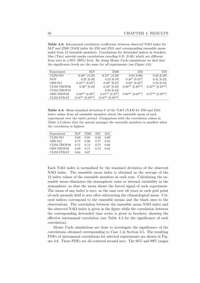
Table 4.3: Interannual correlation coefficients between observed NAO index forSLP and Z500 (NAM index for Z50 and Z10) and corresponding ensemble meanindex from 12 ensemble members. Correlations for detrended indices in brackets.One (Two) asterisk marks correlations exeeding 0.31 (0.40) which are differentfrom zero at a 95% (99%) level. By doing Monte Carlo simulations we find thatthe significance levels are the same for all experiments (see Figure 4.6).
Experiment SLP Z500 Z50 Z10
CLIM-NO -0.36* [-0.29] -0.35* [-0.29] 0.03 [0.06] 0.20 [0.20]NOV 0.25 [0.20] 0.23 [0.19] 0.34* [0.33*] 0.21 [0.22]OBS-NO 0.45** [0.35*] 0.36* [0.27] 0.32* [0.32*] 0.16 [0.16]CLIM-TROP20 0.36* [0.29] 0.33* [0.29] 0.46** [0.49**] 0.42** [0.43**]CLIM-TROP10 0.29 [0.24]OBS-TROP20 0.50** [0.38*] 0.45** [0.37*] 0.60** [0.63**] 0.57** [0.58**]CLIM-STRAT 0.54** [0.59**] 0.54** [0.59**]
Table 4.4: Mean standard deviation σ of the NAO (NAM for Z50 and Z10)index values from all ensemble members about the ensemble mean of eachexperiment over the entire period. Comparison with the correlation values inTable 4.3 shows that the spread amongst the ensemble members is smallest whenthe correlation is highest.
Experiment SLP Z500 Z50 Z10
CLIM-NO 0.80 0.85 0.82 0.69OBS-NO 0.75 0.80 0.77 0.65CLIM-TROP20 0.71 0.74 0.75 0.66OBS-TROP20 0.69 0.71 0.73 0.62CLIM-STRAT 0.64 0.67
Each NAO index is normalised by the standard deviation of the observedNAO index. The ensemble mean index is obtained as the average of the12 index values of the ensemble members in each year. Calculating the en-semble mean eliminates the atmospheric noise or internal variability in theatmosphere, so that the mean shows the forced signal of each experiment.The mean of any index is zero, as the sum over all years at each grid pointof each anomaly field is zero after subtracting the climatological mean. Col-ored indices correspond to the ensemble means and the black ones to theobservations. The correlation between the ensemble mean NAO index andthe observed NAO index is given in the figure while the correlation betweenthe corresponding detrended time series is given in brackets, showing theeffective interannual correlation (see Table 4.3 for the significance of eachcorrelation).
Monte Carlo simulations are done to investigate the significance of thecorrelations obtained corresponding to Case 1 in Section 3.5. The resultingPDFs of interannual correlations for selected experiments are shown in Fig-ure 4.6. These PDFs are all centered around zero. The 95% and 99% ranges

4.1. SEASONAL FORECASTING 35
−1 −0.8 −0.6 −0.4 −0.2 0 0.2 0.4 0.6 0.8 10
500
CLIM−NO
−1 −0.8 −0.6 −0.4 −0.2 0 0.2 0.4 0.6 0.8 10
500
OBS−NO
−1 −0.8 −0.6 −0.4 −0.2 0 0.2 0.4 0.6 0.8 10
500
CLIM−TROP20
−1 −0.8 −0.6 −0.4 −0.2 0 0.2 0.4 0.6 0.8 10
500
OBS−TROP20
−1 −0.8 −0.6 −0.4 −0.2 0 0.2 0.4 0.6 0.8 10
500
CLIM−STRAT
correlation (observed NAO, model NAO)
Figure 4.6: The histograms of correlations between the artificial ensemble meanNAO indices generated by the Monte Carlo method (10, 000 indices; Case 1 inSection 3.5) and the observed NAO index at 500hPa (blue bars). Black dashedlines indicate the median as well as the 95% and the 99% ranges of thedistribution, the boundaries being used as the significance levels of thecorrelations. All correlations of the original ensemble means shown here (greenlines) are significant. Also compare with Figure 4.11 which shows that thesignificance levels are the same also for the correlations between PNA indices.

36 CHAPTER 4. RESULTS
Table 4.5: Number of years (out of 42) when the NAO (NAM in thestratosphere) forecast of the ensemble mean has the correct sign. Values are givenfor all experiments and for our standard quantities. The percentage of winterswith a correct ensemble mean forecast of the sign of the NAO is given in brackets.Largest values are bold.
Experiment SLP Z500 Z50 Z10
CLIM-NO 15 (36%) 18 (43%) 21 (50%) 23 (55%)NOV 22 (52%) 23 (55%) 27 (64%) 26 (62%)OBS-NO 25 (60%) 21 (50%) 26 (62%) 23 (55%)CLIM-TROP20 25 (60%) 24 (57%) 30 (71%) 30 (71%)OBS-TROP20 25 (60%) 25 (60%) 29 (69%) 31 (74%)CLIM-STRAT 28 (67%) 26 (61%)
Table 4.6: The same but for the ensemble members
Experiment SLP Z500 Z50 Z10
CLIM-NO 227 (45%) 236 (47%) 256 (51%) 269 (53%)OBS-NO 275 (55%) 264 (52%) 274 (54%) 266 (53%)CLIM-TROP20 273 (54%) 274 (54%) 287 (57%) 299 (59%)OBS-TROP20 289 (57%) 273 (55%) 305 (61%) 321 (64%)CLIM-STRAT 286 (57%) 292 (58%)
as well as the medians of the distributions are calculated and given in thefigure. For example, the 99% range is obtained by calculating the 0.5% and99.5% percentiles as boundaries so that 99% of the values sit within thoseboundaries. It can be seen that the thresholds do not differ substantially forthe different experiments and we can determine the 95% (99%) significancelevel at a correlation of ρ95 = 0.31 (ρ99 = 0.40) for the following discussion(cf., Figure 4.11: same results for the PNA). Also the November persistenceexperiment NOV has been tested by shuffling the years and the same resultwas obtained. The term “significant at x%” is used to indicate that thecorrelation falls outside the x% range in our discussion, if not differentlyspecified. The results agree with a Students t-test if 42 degrees of freedomare assumed for the test.
The grey shadings in Figure 4.5 mark two standard deviations (STDs)of the ensemble members from the ensemble mean and therefore representthe spread amongst them. In Table 4.3 the interannual correlations for theensemble means for all heights and all experiments are summarised includ-ing their significance while in Table 4.4 the mean STDs for the variabilityamongst the ensemble members about the ensemble mean over all years isnoted as an indication of the spread. Table 4.5 shows the number and thepercentage of years in which the ensemble mean NAO index has the correctsign and Table 4.6 likewise for single realisations.
In Figure 4.7 the results from Monte Carlo simulations corresponding toCase 3 on page 26 in Section 3.5 are presented. 10, 000 single realisations

4.1. SEASONAL FORECASTING 37
−1 −0.8 −0.6 −0.4 −0.2 0 0.2 0.4 0.6 0.8 10
500
CLIM−NO
−1 −0.8 −0.6 −0.4 −0.2 0 0.2 0.4 0.6 0.8 10
500
OBS−NO
−1 −0.8 −0.6 −0.4 −0.2 0 0.2 0.4 0.6 0.8 10
500
CLIM−TROP20
−1 −0.8 −0.6 −0.4 −0.2 0 0.2 0.4 0.6 0.8 10
500
OBS−TROP20
−1 −0.8 −0.6 −0.4 −0.2 0 0.2 0.4 0.6 0.8 10
500
CLIM−STRAT
correlation (observed NAO, model NAO)
Figure 4.7: The histograms of correlations between the NAO indices of 10, 000possible realisations and the observed NAO index at 500hPa (blue bars) none ofwhich was detrended. In contrast to the derivation of the significance levels usedto produce Figure 4.6 the years are kept here during shuffling and correlations arecalculated for the NAO index of single realisations and the observed NAO index(see Case 3 in Section 3.5). Black dashed lines indicate the median as well as the95% and the 99% ranges of the distribution. Green line is the correlation of theensemble mean.
of the NAO index are generated whilst keeping the years of each value fixedcorresponding to possible realisations of the atmosphere of the model ineach winter. The PDF of correlations between the model NAO index andthe observed NAO index is shown. The strength of the forcings can be seenin the displacement of the center of the PDF from zero.
In the first panel (a) of Figure 4.5 the November anomaly persistence“experiment” (NOV) is compared with the observed NAO index. The cor-relation with the observed NAO index of ρ = 0.23 is not significant at the95% level even though in some years and periods the persistence of Novem-ber anomalies resembles well the winter mean NAO, for example in the early1970s or in the mid 1990s. The correlation value for the detrended time se-ries (in brackets) is smaller which indicates that the trend of November NAOvalues had the same sign as the trend of the winter mean NAO between 1961

38 CHAPTER 4. RESULTS
and 2002. In Section 4.2 the trends will be further investigated. Only slightlymore than 50% of the November persistence NAO forecast values have theright sign (see Tables 4.5 and 4.6), meaning that there is no forecasting skillin this method.
At 500hPa the ensemble mean of OBS-NO (Figure 4.5, (b)) is signifi-cantly correlated with the observed NAO index (ρ = 0.36) at the 95% levelonly if the time series are not detrended. The effective interannual corre-lation is not significant (ρ = 0.27). However, the observations are alwayswithin the spread (2 STD) of the ensemble members and so are a possiblerealisation in the experimental setup. These results are similar for the trop-ical relaxation ensemble CLIM-TROP20 ((c), ρ = 0.29 for the detrendedtime series). At SLP the correlations are higher for OBS-NO and CLIM-TROP20 and are still significant if the time series are detrended (see Table4.3). The ratio of a correct forecast of the sign of the NAO is slightly higherfor CLIM-TROP20 than for OBS-NO at both SLP and Z500 (52% to 62%,see Tables 4.5 and 4.6). In Figure 4.7, the PDFs for correlations between theNAO index of single realisations and the observed NAO index for OBS-NOand CLIM-TROP20 are both centered around a value of slightly smallerthan ρ = 0.2 which is a lower correlation than that of the ensemble mean.This is in agreement with Bretherton and Battisti (2000) who state thatthe ensemble mean of a model experiment with a forcing obtained from ob-servations will always have a larger correlation with the observations thanits single members (as can be seen for all experiments). It follows that onthe basis of the analysis so far, knowledge of global SSTSI for any givenwinter is roughly equivalent to having a perfect knowledge of the tropics fordetermining the winter mean NAO index. This means also, however, thatthe distinct influences of the tropics and SSTSI, if seen over all 42 winters,are not particularly strong.
The ensemble OBS-TROP20 (shown in Figure 4.6 and Table 4.3) showsthe combined effect of relaxing the tropics and prescribing extratropicalSSTSI. The interannual correlation of its ensemble mean with the observedNAO index is significant at 95% (ρ = 0.37) which is higher than that ofCLIM-TROP20 but also lower than that of CLIM-STRAT. Also in singlerealisations (Figure 4.7) both forcings add to each other in OBS-TROP20,resulting in an average correlation, between the NAO index obtained fromsingle realisations and the observed NAO index, of slightly less than 0.3.Prescribing a known evolution of extratropical SSTSI therefore adds skill tothe forecast of the NAO index compared to CLIM-TROP20 in which thetropics are perfectly forecasted. This is also reflected by the fact that thereare only very few negative correlation values for OBS-TROP20 in Figure4.7. However, the sign of the NAO forecast is not correct in more than 60% of the years, regarding the ensemble mean (Table 4.5).
The highest interannual correlation is found between the ensemble meanof CLIM-STRAT and the observed NAO index at 500hPa (Figure 4.5, (d),

4.1. SEASONAL FORECASTING 39
ρ = 0.59) which is significant at the 99% level. Even though the spread ofthis ensemble is smallest in the average, the observed NAO index is alwayswithin the spread of the CLIM-STRAT ensemble members in Figure 4.5. Inabout two third of the years, the ensemble mean NAO forecast of CLIM-STRAT at SLP has the same sign as the observed NAO index (Table 4.5).The average correlations between single realisations and the observations(shown in Figure 4.7) for this experiment are around ρ = 0.3, slightly higherthan those of OBS-TROP20. This indicates that the stratospheric forcingfor the NAO is slightly stronger compared to that of OBS-TROP20 (tropicalforcing + extratropical SSTSI). This is also visible in Figure 4.7, as the PDFfor CLIM-STRAT is the narrowest of all experiments and very few singlecorrelations are negative or near zero which means they are very unlikely.The stratospheric relaxation therefore still has the largest impact on thevariability of the NAO compared to the other forcings. This confirms theexpectation of Scaife et al. (2005) that interannual variations of the NAOare reproduced if the stratosphere is relaxed toward observations.
It is noticeable that in general the average spread in the NAO index ofthe realisations in one year is smaller the higher the correlation with theobserved index is. OBS-NO is an exception with higher correlation than forexample CLIM-TROP20 but with a larger spread. The large spread in thesecases may be connected to the fact that in these experiments no relaxationis applied and the atmosphere has more freedom to evaluate.
In the stratosphere, tropical relaxation in CLIM-TROP20 and OBS-TROP20 leads to significant interannual correlations between the ensemblemean NAM index and the observed NAM index which are all significant atthe 99% level (Table 4.3, ρ ≈ 0.60). The correlations for OBS-TROP20 areslightly higher, indicating that SSTSI impact the stratosphere on interan-nual time scales. Seen as ensemble means, the tropical relaxation experi-ments manage to correctly forecast the sign of the NAM in 70% to 80% ofthe 42 years (60%-70% for the single realisations, see Tables 4.5 and 4.6).It has to be kept in mind that the tropical stratosphere is relaxed in CLIM-TROP20 and OBS-TROP20 so that the stratosphere is directly affected inthe tropics. The coincidence of a strong impact of the tropical relaxationensembles on the extratropical stratosphere and the high correlation of theCLIM-STRAT ensemble mean NAO index with the observed NAO indexcan be a hint that the influence of tropical relaxation on the extratropicaltroposphere is via the extratropical stratosphere.
The CLIM-NO experiment is the “control” ensemble, which has no ex-ternal forcing except the climatological seasonal cycle of SST and solar in-solation. Therefore, no interannual correlation is expected between NAOindices from this experiment and the observations. Here a negative corre-lation between the original ensemble mean NAO index and the observedNAO index is found to be significant at the 95% level, but not significant forthe effective interannual correlation, i.e. after detrending (Table 4.3, Z500:
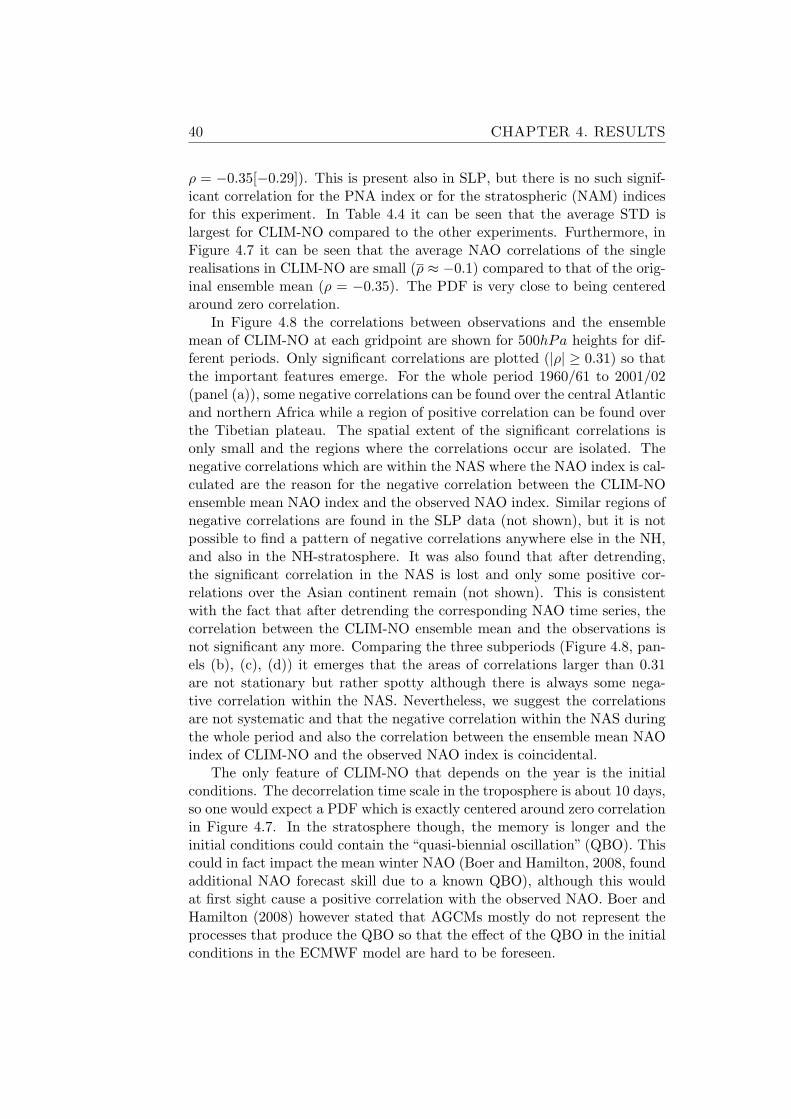
40 CHAPTER 4. RESULTS
ρ = −0.35[−0.29]). This is present also in SLP, but there is no such signif-icant correlation for the PNA index or for the stratospheric (NAM) indicesfor this experiment. In Table 4.4 it can be seen that the average STD islargest for CLIM-NO compared to the other experiments. Furthermore, inFigure 4.7 it can be seen that the average NAO correlations of the singlerealisations in CLIM-NO are small (ρ ≈ −0.1) compared to that of the orig-inal ensemble mean (ρ = −0.35). The PDF is very close to being centeredaround zero correlation.
In Figure 4.8 the correlations between observations and the ensemblemean of CLIM-NO at each gridpoint are shown for 500hPa heights for dif-ferent periods. Only significant correlations are plotted (|ρ| ≥ 0.31) so thatthe important features emerge. For the whole period 1960/61 to 2001/02(panel (a)), some negative correlations can be found over the central Atlanticand northern Africa while a region of positive correlation can be found overthe Tibetian plateau. The spatial extent of the significant correlations isonly small and the regions where the correlations occur are isolated. Thenegative correlations which are within the NAS where the NAO index is cal-culated are the reason for the negative correlation between the CLIM-NOensemble mean NAO index and the observed NAO index. Similar regions ofnegative correlations are found in the SLP data (not shown), but it is notpossible to find a pattern of negative correlations anywhere else in the NH,and also in the NH-stratosphere. It was also found that after detrending,the significant correlation in the NAS is lost and only some positive cor-relations over the Asian continent remain (not shown). This is consistentwith the fact that after detrending the corresponding NAO time series, thecorrelation between the CLIM-NO ensemble mean and the observations isnot significant any more. Comparing the three subperiods (Figure 4.8, pan-els (b), (c), (d)) it emerges that the areas of correlations larger than 0.31are not stationary but rather spotty although there is always some nega-tive correlation within the NAS. Nevertheless, we suggest the correlationsare not systematic and that the negative correlation within the NAS duringthe whole period and also the correlation between the ensemble mean NAOindex of CLIM-NO and the observed NAO index is coincidental.
The only feature of CLIM-NO that depends on the year is the initialconditions. The decorrelation time scale in the troposphere is about 10 days,so one would expect a PDF which is exactly centered around zero correlationin Figure 4.7. In the stratosphere though, the memory is longer and theinitial conditions could contain the “quasi-biennial oscillation” (QBO). Thiscould in fact impact the mean winter NAO (Boer and Hamilton, 2008, foundadditional NAO forecast skill due to a known QBO), although this wouldat first sight cause a positive correlation with the observed NAO. Boer andHamilton (2008) however stated that AGCMs mostly do not represent theprocesses that produce the QBO so that the effect of the QBO in the initialconditions in the ECMWF model are hard to be foreseen.

4.1. SEASONAL FORECASTING 41 1
20o W
60 oW
0o
60
o E
120 oE
180oW
30oN
45oN
60oN
75oN
r(CLIM−NO,ERA−40); (a) 61−02
120
o W
60 oW
0o
60
o E
120 oE
180oW
30oN
45oN
60oN
75oN
(b) 61−81
120
o W
60 oW
0o
60
o E
120 oE
180oW
30oN
45oN
60oN
75oN
(c) 71−91
120
o W
60 oW
0o
60
o E
120 oE
180oW
30oN
45oN
60oN
75oN
(d) 82−02
Figure 4.8: Point correlation r between the evolution of winter mean 500hPageopotential heights of the ensemble mean of CLIM-NO and the reanalysisERA-40 for the periods: (a) 1960/61 - 2001/02, not detrended;all following are detrended: (b) 1960/61 - 1980/81, (c) 1970/71 - 1990/91 and (d)1981/82 - 2001/02. Only correlations larger than |ρ| ≥ 0.31 have been plottedwith a contour interval of 0.05 (based on the 95% significance level for 42 yearstime series obtained from Monte Carlo simulations, see Figure 4.6; note that thesignificance levels would ). The negative correlation over the central Atlantic andnorthern Africa can be the reason for the negative correlation between the NAOindex of CLIM-NO and the observed NAO index.

42 CHAPTER 4. RESULTS
Table 4.7: Like Table 4.3, but for correlations of PNA indices. One (Two)asterisk marks correlations exeeding the 95% (99%) significance levels.
Experiment SLP Z500
CLIM-NO 0.04 [0.04] 0.07 [0.08]NOV 0.13 [0.12] 0.26 [0.25]OBS-NO 0.47** [0.48**] 0.53** [0.58**]CLIM-TROP20 0.80** [0.80**] 0.79** [0.79**]CLIM-TROP10 0.53 [0.58]OBS-TROP20 0.78** [0.79**] 0.77** [0.80**]CLIM-STRAT 0.11 [0.11] 0.04 [0.07]
Table 4.8: Mean standard deviation σ of the PNA index values from theensemble mean for all ensemble members within each experiment over the entireperiod indicating the spread of the PNA indices between the single ensemblemembers.
Experiment SLP Z500
CLIM-NO 0.86 0.77OBS-NO 0.81 0.72CLIM-TROP20 0.63 0.55OBS-TROP20 0.61 0.52CLIM-STRAT 0.83 0.76
4.1.2 Analysis of PNA indices
Figure 4.9 shows the PNA ensemble mean indices of selected experimentscompared to the observed PNA index at 500hPa, similar to Figure 4.5 forthe NAO (see figure caption and Section 2.4 for details of the definition ofthe PNA index). The grey shading again denotes two standard deviationsof the ensemble members of the ensemble mean. Additionally to the latterfigure, El Nino winters are marked with green circles on the observed PNAindex time series. Table 4.7 summarizes the interannual correlations betweenthe ensemble mean PNA indices and the observed PNA index and Table 4.8summarizes the spread (i.e., the average STD) of the ensemble membersabout the ensemble mean respectively. In Figure 4.10 the Monte CarloPDFs of correlations between the single realisations of the PNA index (Case3, Section 3.5) and the observed PNA index are shown. Tables 4.9 and 4.10give the number and the fraction of PNA forecasts with a correct sign for allensemble means and single realisations of the experiments. The significancelevels of the correlations are obtained the same way as for the NAO indicesso that a correlation of ρ95 = 0.31 (ρ99 = 0.40) corresponds to the 95%(99%) significance levels (see Figure 4.11).
The PNA indices obtained from CLIM-NO have no correlation with theobserved PNA index in the average and also have the largest spread com-pared to the other experiments. The ensemble mean PNA index of CLIM-

4.1. SEASONAL FORECASTING 43
1960 1965 1970 1975 1980 1985 1990 1995 2000
−2
0
2
(b) OBS−NO
r= 0.53 [0.58]
1960 1965 1970 1975 1980 1985 1990 1995 2000
−2
0
2
(a) NOV
r = 0.26 [0.25]
1960 1965 1970 1975 1980 1985 1990 1995 2000
−2
0
2
(c) CLIM−TROP20
r= 0.79 [0.79]
1960 1965 1970 1975 1980 1985 1990 1995 2000
−2
0
2
(d) CLIM−STRAT
r = 0.04 [0.07]
Figure 4.9: Like Figure 4.5 but for the PNA index (black) at 500hPa. The PNAindex for observations is obtained as the weighted area mean of 500hPageopotential heights from 30◦N − 65◦N and 160◦E − 140◦W . Green circles markpositive El Nino years (≥ 1STD of DJF mean Nino 3.4 SST index as in Figure2.8).

44 CHAPTER 4. RESULTS
−1 −0.8 −0.6 −0.4 −0.2 0 0.2 0.4 0.6 0.8 10
500
CLIM−NO
−1 −0.8 −0.6 −0.4 −0.2 0 0.2 0.4 0.6 0.8 10
500
OBS−NO
−1 −0.8 −0.6 −0.4 −0.2 0 0.2 0.4 0.6 0.8 10
500
CLIM−TROP20
−1 −0.8 −0.6 −0.4 −0.2 0 0.2 0.4 0.6 0.8 10
500
OBS−TROP20
−1 −0.8 −0.6 −0.4 −0.2 0 0.2 0.4 0.6 0.8 10
500
CLIM−STRAT
correlation (observed PNA, model PNA)
Figure 4.10: Like Figure 4.7, but for correlations between the PNA indices ofobservations and ensemble members at 500hPa none of which was detrended. Itcan be seen that the astonishingly high correlations between the ensemble meanPNA index of CLIM-TROP and OBS-TROP20 are supported by the fact that thePDFs of correlations are far away from zero correlation which appears to beimpossible if tropical relaxation is applied. CLIM-STRAT however yields a PDFsimilar to that of CLIM-NO meaning that the stratospheric is unimportant for thePNA.

4.1. SEASONAL FORECASTING 45
Table 4.9: Number of years (out of 42) when the PNA forecast, based on theensemble mean, has the correct sign. The percentage of winters with a correctforecast of the sign of the PNA is given in brackets. Values are given for allexperiments and for our standard quantities. Largest values are bold.
Experiment SLP Z500
CLIM-NO 22 (52%) 22 (52%)NOV 24 (57%) 29 (69%)OBS-NO 32 (76%) 31 (74%)CLIM-TROP20 38 (91%) 34 (81%)OBS-TROP20 36 (86%) 33 (79%)CLIM-STRAT 23 (55%) 21 (50%)
Table 4.10: The same but for the ensemble members
Experiment SLP Z500
CLIM-NO 254 (50%) 247 (49%)OBS-NO 316 (63%) 320 (63%)CLIM-TROP20 387 (77%) 364 (72%)OBS-TROP20 373 (74%) 360 (71%)CLIM-STRAT 257 (51%) 236 (47%)
NO has no correlation with the observed PNA index (ρ = 0.07). Consis-tently, the PDF of correlations of shuffled PNA realisations (Figure 4.10)is centered around zero and has the widest distribution amongst all experi-ments.
It can be seen that observed SSTSI in OBS-NO at the lower boundaryleads to a significant interannual correlation between the ensemble meanPNA index and the observed PNA index (ρ = 0.53, at 99% level). Thisis caused mainly by the last third of the period (ρ≥1988 = 0.76), in thefirst third there is only little correlation (ρ≤1975 = 0.19). The spread of theensemble members is smaller than that of the CLIM-NO experiment andabout two third of the PNA forecasts of OBS-NO have the right sign. Forthe variability of the PNA, prescribing SST is very influential, an influencewhich is probably via the atmospheric bridge (Alexander et al., 2002).
The tropical relaxation ensemble CLIM-TROP20 produces winter meanPNA values which are highly correlated with the observed PNA index atthe 99% level (ρ = 0.79). The correlation is high over the whole periodand in years of El Nino events the agreement between the ensemble meanof CLIM-TROP20 and the observed PNA index is astonishingly high (ex-cept for the 1965/1966 and 1986/1987 El Ninos). Also analysing SLP, thecorrelation between the observed PNA index and ensemble mean index isvery high (ρ = 0.80). The results are not particular sensitive to a slightchange of the relaxation region, as the correlations are still significant forthe CLIM-TROP10 experiment (ρ = 0.53). It has to be kept in mind thatin the CLIM-TROP10 ensemble only 4 members were executed which is not

46 CHAPTER 4. RESULTS
sufficient to completely average out the atmospheric noise. Additionally thespread amongst the ensemble members is much lower for CLIM-TROP20than for CLIM-NO, indicating the strong influence of the tropical forcing.The impact of the tropical relaxation for the PNA can be clearly seen inFigure 4.10. Both the PDFs of CLIM-TROP and of OBS-TROP20 real-isations are centered around a correlation larger than ρ = 0.6 and valuessmaller than ρ = 0.4 are outside the 99% range of both PDFs. It is alsoevident that extratropical SSTSI add some skill to the tropical relaxationexperiment, be it only slightly. This in turn implies that in OBS-NO, theforecasting skill is caused mainly by adding tropical SST. These results areconsistent with those of Newman et al. (2003) who note, based on observa-tions, that the PDO is dependent on ENSO on all time scales and that the(oceanic) PDO is directly correlated to the (atmospheric) PNA in winter.
The stratospheric relaxation ensemble CLIM-STRAT does not lead tosignificant correlations in the Pacific sector. Its ensemble mean PNA indexis correlated to the observed one with ρ = 0.04 at 500hPa (ρ = 0.11 in SLP).Also the spread between the members is not really smaller than those of theensemble without any forcing, CLIM-NO. The weak impact is also visible inFigure 4.10 where the PDF of CLIM-STRAT realisations is nearly identicalto that of CLIM-NO except that it is slightly narrower. The results areconsistent with the results of the pattern correlation analysis (see Figure 4.4and Table 4.1). The stratospheric relaxation causes a marginal improvementof the pattern correlations in the NPS compared to CLIM-NO. Only thestrong kurtosis of the pattern correlations of CLIM-STRAT within the NPSin Figure 4.4 cannot be retrieved in the analysis of the PNA indices.
It can be seen that detrending of the time series does not influence thesignificance of the correlations associated to the PNA, in contrast to the re-sults for the NAO described in the previous section. This is in the first placedue to the fact that the correlations are more pronounced (no correlation forCLIM-NO and CLIM-STRAT, high correlations for OBS-NO, CLIM-TROPand OBS-TROP20), but also because the trend of the PNA index duringthe period 1960/61 to 2001/02 is less strong than that of the NAO duringthe same period (see Section 4.2).
The tropical atmosphere and the evolution of tropical SST, both proba-bly mainly in the Pacific region, have the largest impact on the interannualvariability of the PNA. A better forecast of the tropics would thus enhancethe seasonal predictability of anomalous winter mean circulations in the ex-tratropical troposphere in the NPS.

4.1. SEASONAL FORECASTING 47
−1 −0.8 −0.6 −0.4 −0.2 0 0.2 0.4 0.6 0.8 10
500
CLIM−NO
−1 −0.8 −0.6 −0.4 −0.2 0 0.2 0.4 0.6 0.8 10
500
OBS−NO
−1 −0.8 −0.6 −0.4 −0.2 0 0.2 0.4 0.6 0.8 10
500
CLIM−TROP20
−1 −0.8 −0.6 −0.4 −0.2 0 0.2 0.4 0.6 0.8 10
500
OBS−TROP20
−1 −0.8 −0.6 −0.4 −0.2 0 0.2 0.4 0.6 0.8 10
500
CLIM−STRAT
correlation (observed PNA, model PNA)
Figure 4.11: Like Figure 4.6, but for correlations of PNA indices at 500hPa.The significance levels are approximately the same for all experiments and alsothe same as for the NAO.

48 CHAPTER 4. RESULTS
4.2 Trends during the ERA-40 period
As mentioned in Chapter 2, a climate regime shift was detected duringthe late 1970s in the Pacific sector (Trenberth et al., 2002), changing thevariability of teleconnection patterns like the PNA (Greatbatch et al., 2004).On the other hand, the NAO index went through a positive trend from theearly 1970s to the mid 1990s and there is disagreement about the originsof this trend in model simulations. It is consistent with being generatedjust by chance due to internal variability of the coupled climate system(Semenov et al., 2008). Also changing conditions in single components ofthe system could be the reason, e.g. in the tropics (Lu et al., 2004), in thestratosphere (Scaife et al., 2005), as well as in low frequency ocean dynamics.Here, possible origins of trends in the winter NAO and PNA indices areinvestigated using the relaxation experiments described in Section 2.2.1.
As a first step, the patterns of the ensemble mean trends in 500hPageopotential heights are compared to the observed one in Figure 4.12. Theobserved linear trend in 500hPa in winters from 1961 to 2002 exhibits deep-enings of the Icelandic (≈ −20m/10yr) and the Aleutian (≈ −20m/10yr)troughs, deepening geopotential over Russia (≈ −15m/10yr) and risinggeopotential heights over East Asia (≈ +5m/10yr), North America (≈+10m/10yr) and Europe (≈ +15m/10yr). The observed trend patternstrongly projects on to the NAO and the PNA patterns respectively, sothat it is reasonable to investigate the trends of the respective indices in thefollowing sections. The amplitudes of the trends are slightly stronger thanfound for the period 1949 to 1999 by Lu et al. (2004). Lu et al. (2004) notedthat the pattern of the trend is similar to the “Cold Ocean Warm Land”(COWL) pattern of Wallace et al. (1995). The trend pattern looks similarfor SLP (not shown).
The ensemble mean linear trends from our model experiments have asmaller amplitude compared to the observations. Hence, the contour intervalfor the ensemble mean trends in Figure 4.12 is reduced by 1/4 compared tothe observations to allow for a comparison of the patterns. OBS-NO, CLIM-TROP20 and OBS-TROP20 reveal similar trend patterns to that observedin our period. OBS-NO has the wrong trend sign in the NPS so that despitea very good accordance in the NAS, the trend pattern correlation over theNH north of 30oN is only ρpc = 0.36. The trend of CLIM-TROP20 ishigher correlated overall to the observed trend (ρpc = 0.41) and only failsto represent the trend over North America and Central Asia. The bestaccordance can be found for the OBS-TROP20 ensemble (ρpc = 0.63) whichyields weak deficiencies only over the Asian continent. These results aresimilar to that of Lu et al. (2004) who used a simple dynamical model toexamine the influence of trends in the tropics on extratropical troposphericcirculation trends.
There is no accordance of trends between the ensemble mean of CLIM-
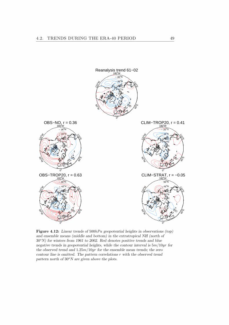
4.2. TRENDS DURING THE ERA-40 PERIOD 49
120
o W
60 oW
0o
60
o E
120 oE
180oW
36oN
48oN
60oN
72oN
84oN
Reanalysis trend 61−02
120
o W
60 oW
0o
60
o E
120 oE
180oW
36oN
48oN
60oN
72oN
84oN
OBS−NO, r = 0.36
120
o W
60 oW
0o
60
o E
120 oE
180oW
36oN
48oN
60oN
72oN
84oN
CLIM−TROP20, r = 0.41
120
o W
60 oW
0o
60
o E
120 oE
180oW
36oN
48oN
60oN
72oN
84oN
OBS−TROP20, r = 0.63
120
o W
60 oW
0o
60
o E
120 oE
180oW
36oN
48oN
60oN
72oN
84oN
CLIM−STRAT, r = −0.05
Figure 4.12: Linear trends of 500hPa geopotential heights in observations (top)and ensemble means (middle and bottom) in the extratropical NH (north of30oN) for winters from 1961 to 2002. Red denotes positive trends and bluenegative trends in geopotential heights, while the contour interval is 5m/10yr forthe observed trend and 1.25m/10yr for the ensemble mean trends; the zerocontour line is omitted. The pattern correlations r with the observed trendpattern north of 30oN are given above the plots.

50 CHAPTER 4. RESULTS
120
o W
60 oW
0o
60
o E
120 oE
180oW
36oN
48oN
60oN
72oN
84oN
Reanalysis trend 65−95
120
o W
60 oW
0o
60
o E
120 oE
180oW
36oN
48oN
60oN
72oN
84oN
OBS−NO, r = 0.57
120
o W
60 oW
0o
60
o E
120 oE
180oW
36oN
48oN
60oN
72oN
84oN
CLIM−TROP20, r = 0.7
120
o W
60 oW
0o
60
o E
120 oE
180oW
36oN
48oN
60oN
72oN
84oN
OBS−TROP20, r = 0.76
120
o W
60 oW
0o
60
o E
120 oE
180oW
36oN
48oN
60oN
72oN
84oN
CLIM−STRAT, r = 0.6
Figure 4.13: Like Figure 4.12, but for the sub-period 1964/65 to 1994/95. Reddenotes positive trends and blue negative trends in geopotential heights, while thecontour interval is 5m/10yr for observed trend and 1.25m/10yr for the ensemblemean trends; the zero contour line is omitted.

4.2. TRENDS DURING THE ERA-40 PERIOD 51
120
o W
60 oW
0o
60
o E
120 oE
180oW
30oN
45oN
60oN
75oN
z50, 61−02 trend, contour = 10 m/10y
120
o W
60 oW
0o
60
o E
120 oE
180oW
30oN
45oN
60oN
75oN
z50, 65−95 trend
120
o W
60 oW
0o
60
o E
120 oE
180oW
30oN
45oN
60oN
75oN
z10, 61−02 trend, contour = 10 m/10y
120
o W
60 oW
0o
60
o E
120 oE
180oW
30oN
45oN
60oN
75oN
z10, 65−95 trend
Figure 4.14: The observed trends in mean winter geopotential heights in thestratosphere. Contour interval is m/yr while red means positive and blue negativewhile the zero contour line is omitted. First row shows the trends at 50hPa andsecond the trends at 10hPa. First column gives the trend between 1961 and 2002while second column gives the trend between 1965 and 1995.
STRAT and the observations (ρpc = −0.05) in the NH; in the NPS thetrend pattern is even of the opposite sign compared to the observed trend.This is in contrast to the results of Scaife et al. (2005) who used a differentforcing method to investigate the stratospheric influence on the troposphericdecadal trends between 1965 and 1995 and found a strong impact on the30-year trend in the NAS in SLP. If we analyse our results during the sub-period between 1965 and 1995 (Figure 4.13), we also find a very strongimpact of the stratospheric relaxation in the NAS which strongly projectsonto the NAO. The trend pattern correlation changes from -0.05 (1960/61to 2001/02) to 0.64 (1964/65 to 1994/95) for CLIM-STRAT so that thestratospheric forcing has a similar impact on the hemispheric trend as theother forcings. Our results therefore confirm the findings of Scaife et al.(2005). It is remarkable that the observed trend at Z500 between 1964/65and 1994/95 was about 50% stronger than between 1960/61 and 2001/02(identical contour interval in Figures 4.12 and 4.13). In the NPS, OBS-NOand CLIM-STRAT still yield a trend opposite to the observed trend duringthe sub-period. The ensemble mean of CLIM-NO reveals a trend patternwhich is very weak in either of the periods compared with the other ensemblemean trends and negatively correlated to the observed one (ρpc = −0.46, notshown), but the relatively high correlation value is probably spurious.

52 CHAPTER 4. RESULTS
Table 4.11: Ratios of ensemble mean NAO/NAM trends and observed ERA-40NAO/NAM trend over the period 1960/61 to 2001/02. Values closest to 1 arebold. Observed trends are: SLP: 1.41 σ/42yr; Z500: 1.35 σ/42yr; Z50:0.30 σ/42yr; Z10: −0.11 σ/42yr;
Experiment SLP Z500 Z50 Z10
CLIM-NO -0.14 -0.13 -1.13 1.66NOV 0.32 0.32 1.11 -2.84OBS-NO 0.32 0.31 0.16 -0.87CLIM-TROP20 0.21 0.15 -1.13 3.60OBS-TROP20 0.49 0.40 -1.02 2.95CLIM-STRAT -0.01 >-0.01
The observed trend in the NH stratosphere was significantly strongerin the sub-period between 1965 and 1995 (≈ −8m/yr at Z50 over the pole,Figure 4.14) than in our whole period 1961 to 2002 (≈ −3m/yr at Z50) whenthe trend pattern is also much less annular than in the sub-period (Figure4.14). It is therefore likely that the stratospheric impact on the trends ofgeopotential heights in the NAS in the period 1965 to 1995 is real. However,it is not possible to conclude from the results in which way the impact tookplace in reality, but they confirm the strong connection between troposphereand stratosphere in the NAS in winter.
4.2.1 NAO/NAM
The NAO indices shown in Figure 4.5 are investigated regarding their trends.If σ is one standard deviation (STD) of the observed NAO index values,the NAO trend between 1961 and 2002 was 1.33σ/42yr at 500hPa and1.44σ/42yr in SLP. The ratios of the ensemble mean trends to the observedtrend are given in Table 4.11. In Figure 4.15 the results of the Monte Carloexperiments corresponding to Case 2 on page 25 in Section 3.5 are shownfor 500hPa. It can be examined here if the observed trend can be capturedby the model and the different experimental setups.
Consistent with the negative pattern correlation of ρ = −0.46 over thewhole extratropical NH, it can be seen in Table 4.11 that the“control”CLIM-NO ensemble does not have an NAO trend similar to the observed. The PDFof NAO trends for single realisations is centered around zero and has a verybroad range (Figure 4.15), but the observed NAO trend sits outside the 99%range of the PDF. This is in a way contrary to the results of Semenov et al.(2008) who stated that the positive NAO trend between 1965 and 1995 lieswithin the natural variability of the coupled climate system. They howeverused a fully coupled model with considerably longer and continuous modelruns and looked at slightly different time spans (30 years instead of 42).In the stratosphere at 10hPa the ensemble mean CLIM-NO NAM indexhas a high accordance with the observations showing that the weak negative
4.2. TRENDS DURING THE ERA-40 PERIOD 53
observed NAM trend lies within the scope of atmospheric internal variability.In the North Atlantic sector (NAS) the ensemble mean with tropical re-
laxation (CLIM-TROP20) reveals a trend pattern projecting onto a positiveNAO pattern at 500hPa (see Figure 4.12). The center of the negative trendregion over Greenland is shifted eastwards compared to the observations,still yielding an NAO trend which has the same sign as the observed one.The CLIM-TROP20 ensemble mean NAO index represents 15− 23% of theobserved NAO trend (Table 4.11) and the PDF shown in Figure 4.15 forsingle CLIM-TROP20 realisations is slightly shifted towards the observedNAO trend which however is still outside the 99% range of the PDF.
Historically varying SST and sea-ice (OBS-NO) yield a similar result tothat of tropical relaxation in the ensemble mean but with a slightly strongerNAO trend (≈ 30% of the observed). The observed NAO trend is within the99% range of the PDF here, which is of a similar width as the PDF of theCLIM-NO realisations, but clearly shifted toward the observed trend. Thetrend PDFs of realisations are wider for the experiments without relaxationthan for those with relaxation indicating that the model atmosphere is lessconstrained without relaxation. The observed NAO trend is more likelyto be captured if the evolution of tropical and extratropical SST is known(OBS-NO). However, the region of the negative trend in the NAS is slightlyshifted westward and the region of rising geopotential in the lower latitudesis shifted northward compared to the observations (Figure 4.12).
The ensemble mean NAO index of OBS-TROP20 represents about 40−50% of the linear trend compared to the observed NAO trend, which isalso evident in the trend pattern which is very similar to the observed one.The observed NAO trend is within the 99% range of the PDF of trends ofthat experiment which has a somewhat narrower range than that of OBS-NO. Comparing the PDFs of OBS-NO, CLIM-NO and OBS-TROP20 it isevident that the tropical relaxation has a smaller effect on the NAO trendthan the evolution of extratropical SSTSI as the PDFs of OBS-NO andOBS-TROP20 are very similar.
For the period 1961 to 2002, the stratospheric relaxation experimentCLIM-STRAT reveals a small effect of the stratosphere on the NAO trendboth in the ensemble mean trend pattern and in the magnitude of the trendsof ensemble mean and single realisations. The ensemble mean trend ofCLIM-STRAT is near zero and the trend PDF of realisations in Figure 4.15(left column) is centered around zero with a slightly smaller width com-pared to that of CLIM-NO. As mentioned in the previous section, this iscontrary to the results of Scaife et al. (2005), but if the period of the anal-ysis is restricted to the period between 1965 and 1995 (Figure 4.15, rightcolumn), the ensemble mean NAO index of CLIM-STRAT represents about40% of the observed NAO index and the PDF of trends is shifted toward theobserved trend. Accordingly, the PDF of CLIM-STRAT realisations takenfrom this sub-period has a much smaller width than for the whole period

54 CHAPTER 4. RESULTS
−0.5 0 0.50
500
CLIM−NO, 61−02 trends
−0.5 0 0.50
500
OBS−NO
−0.5 0 0.50
500
CLIM−TROP20
−0.5 0 0.50
500
OBS−TROP20
−0.5 0 0.50
500
CLIM−STRAT
σNAO
/ 10yr
−0.5 0 0.50
500
CLIM−NO, 65−95 trends
−0.5 0 0.50
500
OBS−NO
−0.5 0 0.50
500
CLIM−TROP20
−0.5 0 0.50
500
OBS−TROP20
−0.5 0 0.50
500
CLIM−STRAT
σNAO
/ 10yr
Figure 4.15: Left column: Histograms of 500hPa NAO trends (in units ofstandard deviation per 10 years) between 1961 and 2002 in individual modelrealisations generated as described in Section 3.5. Right column: The same forthe 1965 to 1995 sub-period. Red lines show the observed NAO trend. Blackdashed lines indicate the median as well as the 95% and the 99% ranges of thedistribution.

4.2. TRENDS DURING THE ERA-40 PERIOD 55
Table 4.12: Ratios of ensemble mean PNA trends and observed ERA-40 PNAtrend. Observed trends are: SLP: 0.48 σ/42yr; Z500: 0.75 σ/42yr; Values closestto 1 are bold.
Experiment SLP Z500
CLIM-NO 0.12 -0.05NOV 0.70 0.40OBS-NO -0.02 -0.49CLIM-TROP20 0.32 0.20OBS-TROP20 0.18 -0.13CLIM-STRAT -0.04 -0.18
and is even narrower than those PDFs of the tropical relaxation experimentsduring the sub-period. This indicates that during the 1965-1995 period thestratosphere had a strong impact on the NAO.
Between 1961 and 2002 however, prescribing the evolution of SSTSI(OBS-NO and OBS-TROP) causes trends which have the largest accordancewith the observed trends in the NAS or of the NAO trends respectively.
4.2.2 PNA
The overall trend between 1961 and 2002 of the winter PNA was 0.75 σ/42yr(0.48 σ/42yr at SLP) and is investigated here in the context of the regimeshift in the late 1970s. The corresponding ensemble mean indices can befound in Figure 4.9 and the ratios of the ensemble mean trends to the ob-served trend are shown in Table 4.12 for 500hPa and SLP. The follow-ing descriptions refers to the results of the analysis of 500hPa geopotentialheights. In Figure 4.16 the results of the Monte Carlo experiments is shownto examine the unusualness of the observed PNA trend in selected modelsetups.
For the “control” experiment CLIM-NO we find that the PDF of PNAtrends from the Monte Carlo experiments is centered around zero in Figure4.16, but also that the range of trends of the single members is quite broad.The observed PNA trend therefore lies within the 95% range of trends inthe model setup with climatological seasonal cycle of SST and solar forcing.Internal variability of the extratropical atmosphere can thus not be excludedas a reason for the observed PNA trend.
In previous studies, the tropical Pacific and the tropical atmosphere inthe Pacific sector were found to influence the PNA on different timescales(e.g. Alexander, 1992). A shift to more frequent occurrence of winters with awarm El Nino event was observed after the late 1970s, suggesting a change ofconditions in the tropical Pacific (Trenberth and Hurrell, 1994). Accordingly,our tropical relaxation experiment CLIM-TROP20 produces a trend which,in the ensemble mean, is similar to the observed one in its spatial pattern

56 CHAPTER 4. RESULTS
−0.5 0 0.50
500
CLIM−NO, 61−02 trends
−0.5 0 0.50
500
OBS−NO
−0.5 0 0.50
500
CLIM−TROP20
−0.5 0 0.50
500
OBS−TROP20
−0.5 0 0.50
500
CLIM−STRAT
σPNA
/ 10yr
−0.5 0 0.50
500
CLIM−NO, 65−95 trends
−0.5 0 0.50
500
OBS−NO
−0.5 0 0.50
500
CLIM−TROP20
−0.5 0 0.50
500
OBS−TROP20
−0.5 0 0.50
500
CLIM−STRAT
σPNA
/ 10yr
Figure 4.16: Left column: Histograms of 500hPa PNA trends (in units ofstandard deviations per 10 years) between 1961 and 2002 in individual modelrealisations generated as described in Section 3.5. Right column shows the samefor the 1965 to 1995 sub-period. Red lines show the observed PNA trend. Blackdashed lines indicate the median as well as the 95% and the 99% ranges of thedistribution.
4.2. TRENDS DURING THE ERA-40 PERIOD 57
(see Figure 4.12) and in amplitude of 20− 30% (see Figure 4.16 and Table4.12). In Figure 4.16 it can be seen that the PDF of trends for CLIM-TROP20 realisations is shifted towards the observed PNA trend comparedto the CLIM-NO experiment and the observed trend lies within the 99%range, but slightly outside the 95% range. The origin of the trend of thePNA pattern could therefore be located in the tropics. The wideness of thePDF is small compared to that of CLIM-NO and OBS-NO, indicating astrong influence of the forcing.
The OBS-NO experiment yields a negative ensemble mean PNA trendwhich can be seen by comparing the sign of the trend in the North Pa-cific sector in Figure 4.12 and also in Figure 4.16 where the PDF of trendsfor realisations of this experiment is shifted away from the observed trendcompared to the control experiment CLIM-NO. The observed PNA trendis outside the 99% range of the PDF of OBS-NO trends and the ensemblemean PNA trend has an amplitude of −49% of the observed one (see Ta-ble 4.12). The PDF of trends has large range, similar to that of CLIM-NOsuggesting that the forcing of prescribing observed SST is weak on decadaltime scales in the North Pacific sector (NPS) during the period 1961-2002(the results are similar for the period 1965 to 1995, see Figure 4.16, rightcolumn). Copsey et al. (2006) suggest that atmosphere-only models are de-ficient at correctly representing SLP trends when SSTs are prescribed, forexample in the Indian Ocean region. Indeed, the SLP trend of the OBS-NOensemble mean has, in the Indian Ocean region (30oE - 100oE, 35oN - 35oS),an opposite average trend of SLP (−0.005hPa/10yr) compared to that ob-served (+0.5hPa/10yr). The Indian Ocean has seen a warming trend in ourperiod which has been recognized as a greenhouse gas signal by Hurrell et al.(2004). In the coupled atmosphere-ocean system, conditions of reduced con-vection and increased solar insolation lead to warm SST anomalies whereasatmosphere-only models run with specified SST tend to generate convec-tion and increased precipitation over warm SST anomalies leading to theopposite behavior in the model from what is observed.
The ensemble members with specified observed global SST combinedwith tropical relaxation (OBS-TROP20) yield a PDF of linear PNA trendswith a negative and weak mean trend (Figure 4.16). It therefore lies inbetween the PDFs of OBS-NO and CLIM-TROP20 and the wideness ofthe PDF is small, similar to that of CLIM-TROP20 and the observed PNAtrend is outside the 99% range of the PDF. That suggests that prescribingobserved extratropical SSTSI degrades the PNA trend.
CLIM-STRAT, the ensemble with stratospheric relaxation as a forcingyields a PDF of PNA trends (Figure 4.16) which looks similar to the PDF ofthe control experiment CLIM-NO, with the mean near zero and a relativelywide range so that the observed PNA trend is within the 99% range inthis case and so is a possible realisation in the context of this experiment.However, this result is not independent of the period of interest in so far

58 CHAPTER 4. RESULTS
that between 1965 and 1995, the observed PNA trend is outside the 99%range of trends of CLIM-STRAT realisations (Figure 4.16, right column).The ensemble mean PNA trend has an amplitude of −18% of the observedPNA trend indicating that it has the wrong sign. As shown in Figure 4.12,the ensemble mean trend pattern for CLIM-STRAT is quite of the oppositesign compared to the observations in the NPS.
Chapter 5
Conclusions and discussion
In this study, hindcast experiments were analysed to examine the influenceof different parts of the climate system on the interannual variability andtrends in the winter mean circulation of the extratropical troposphere ofthe northern hemisphere during the ERA-40 period between 1960/61 and2001/02. 500hPa geopotential heights were mainly used for the analysis.The focus of the analysis of the interannual variability has been on theseasonal predictability skill which could be added by assuming perfect pre-dictability in the region of the added forcing. The added forcing of themodel experiments was applied using the relaxation technique (Section 2.2)to constrain the atmosphere toward reanalysis data in different regions, i.e.,the tropics or the stratosphere. Also prescribed observed SST and sea-ice(SSTSI) were used as a forcing for the winter circulation and a “control”experiment with the climatological mean cycle of SSTSI and solar forcingwas analysed.
In the northern hemisphere (NH) as a whole and the North Atlanticsector (NAS) in particular, tropical relaxation (CLIM-TROP20 and OBS-TROP20) adds most forecast skill in our experiments (Section 4.1, Figures4.3 and 4.4). The stratosphere (CLIM-STRAT) however has a larger impacton the NAO related part of the tropospheric circulation variability than doesthe tropical atmosphere (Section 4.1.1). This means that a better represen-tation of the stratosphere, but also the tropical atmosphere, is important forthe seasonal forecast of the NAO. It also confirms that the stratosphere isdynamically important for the NAO related variability in the NAS, be it bythe downward propagation of stratospheric anomalies or by radiative effectsdue to greenhouse gases or ozone. It is also possible that part of the NAOforecast skill which is added by relaxing the tropics is dynamically causedby tropical circulation anomalies propagating poleward, affecting extratrop-ical standing waves, for example in the North Pacific sector which in turnimpact the polar vortex in the stratosphere that in turn impacts the NAO(Ineson and Scaife (2008) suggested this mechanism). Prescribing global
59

60 CHAPTER 5. CONCLUSIONS AND DISCUSSION
SSTSI (OBS-NO) leads to a similar amount of NAO related variability com-pared with the tropical relaxation in CLIM-TROP20. Extratropical SSTSIseem to play a role for the interannual variability of the NAO as the ensem-ble OBS-TROP20 has a larger skill in capturing the interannual variabilitythan CLIM-TROP (see Section 4.1.1, Table 4.3 and Figure 4.7). The vari-ability of the atmospheric circulation in the North Atlantic sector remainsa complex issue and no predominant influence of the climate system can bedetermined. The stratosphere however seems to play a significant role forthe NAO variability and more understanding of stratospheric dynamics andan improved monitoring of its behaviour could be helpful for the predictionof the NAO related fraction of variability (Maycock et al. (2009) also notedthis).
The observed upward trend of the NAO index during our period of in-terest (1961-2002, see Section 4.2.1) is found to be best reproduced by theexperiments with prescribed extratropical SSTSI (in OBS-NO and OBS-TROP20) which yield at least 30% of the magnitude of the observed NAOtrend. Tropical relaxation adds some skill to the representation of the trend.When looking at the sub-period 1965-1995, stratospheric trends were foundto have a considerable contribution to the observed upward trend in theNAO index (in agreement with Scaife et al., 2005), comparable with thecontribution from SSTSI, while this signal is lost when looking at the wholeperiod 1961 to 2002. This suggests that the atmospheric conditions in eitherof the two periods are not directly comparable on decadal time scales andconclusions taken from any 30 or 40-year-period can not be assumed to beuniversally valid.
In the North Pacific sector the tropical atmosphere and the tropical SSTconditions during winter are the most important factors for the interannualvariability (of the PNA) according to our experiments. It was found thatespecially constraining the tropical atmosphere to reanalysis data (CLIM-TROP and OBS-TROP20) powerfully enhances the model performance ingeneral (Section 4.1, Figure 4.4) and also the PNA related part of the vari-ability in this sector in particular (Section 4.1.2, Figures 4.9 and 4.10). Thisis consistent with the strong connection between the PNA and the tropicalPacific which was confirmed in a number of previous studies. The connectionis caused by the poleward propagation of circulation anomalies through theupper troposphere causing an anomalous lower tropospheric circulation andalso anomalous SST conditions in the extratropical North Pacific, called an“Atmospheric Bridge” (Alexander et al., 2002; Newman et al., 2003). It hasto be noted that there is little representation of the observed PNA in theOBS-NO ensemble in the first third of our analysis period (see Figure 4.9),a fact that might be explained by a poor SSTSI observational data qualitybefore the beginning of the satellite era.
The regime shift of the PNA (and related features) to a more positivestate was found to possibly be caused by trends in the tropical atmosphere

61
(see Section 4.2.2, Figure 4.16, CLIM-TROP). This agrees with a trend toa higher occurrence of warm El Nino events, which are known to cause adeeper than usual Aleutian low (Alexander et al., 2002), in the second half ofour period of interest. But also internal atmospheric variability clearly cap-tures the overall trend between 1961 and 2002 (see Figure 4.16). Prescribingobserved SST causes an opposite PNA trend compared to the observations,suggesting that this forcing degrades the model’s ability to reproduce thePNA trend. This result could however be misleading because the atmo-spheric response to SST anomalies in atmosphere-only models (like ours)can in some regions be of the opposite sign relative to the observations(see Copsey et al., 2006). The tropical relaxation however (CLIM-TROP,OBS-TROP20) simulates a perfect coupling of ocean and atmosphere in thetropics and therefore is a good alternative to prescribing tropical SST in anAGCM.
There are a lot of possibilities for further experiments to be looked at, forexample relaxing only parts of the tropics or only the tropical troposphere;also the impact of the extratropics on the tropics can be examined (see Junget al., 2010, 2011; Vitart and Jung, 2010, for further possibilities). Moreanalysis could be done, for example taking a closer look at running trendsduring sub-periods like that between 1965 and 1995, at the variability withinthe stratosphere or the evolution of specific winters like the cold Europeanwinter 1962/63 or the high NAO/low PNA winter of 1988/89.

62 CHAPTER 5. CONCLUSIONS AND DISCUSSION

List of Figures
2.1 ERA-40 model levels . . . . . . . . . . . . . . . . . . . . . . . 5
2.2 ERA-40 Winter (DJF) SLP + Z500 climatology . . . . . . . . 6
2.3 ERA-40 Winter (DJF) Z50 + Z10 climatology . . . . . . . . . 7
2.4 Internal variability of the model by means of the NAO patternobtained by the analysis of the CLIM-NO experiment . . . . 9
2.5 Relaxation coefficient for the stratospheric relaxation . . . . . 11
2.6 NAO/NAM indices from observations . . . . . . . . . . . . . 14
2.7 NAO pattern for SLP + Z500 . . . . . . . . . . . . . . . . . . 15
2.8 PNA/NPI indices from observations . . . . . . . . . . . . . . 17
2.9 PNA pattern for Z500 . . . . . . . . . . . . . . . . . . . . . . 18
3.1 SLP anomalies for 1962/1963 as an explanation of the patterncorrelation . . . . . . . . . . . . . . . . . . . . . . . . . . . . . 24
4.1 Schematic summary of the results of the correlation analysis . 28
4.2 Schematic summary of the results of the analysis of NAO/PNAtrends . . . . . . . . . . . . . . . . . . . . . . . . . . . . . . . 28
4.3 Pattern correlation histograms, NH, CLIM-NO, NOV, CLIM-TROP and CLIM-STRAT . . . . . . . . . . . . . . . . . . . . 30
4.4 Pattern correlation histograms, NAS and the NPS for OBS-NO, CLIM-TROP20, OBS-TROP20 and CLIM-STRAT . . . 31
4.5 Ensemble mean NAO compared with observed NAO for 500hPa 33
4.6 PDF of NAO correlations between the NAO index of shuffledensemble means and the observed NAO index at 500hPa . . 35
4.7 PDF of NAO correlations between the NAO index of possiblerealisations and the observed NAO index at 500hPa . . . . . 37
4.8 Point correlation between CLIM-NO and observations at 500hPaduring 1960/61-2001/02 and three sub-periods . . . . . . . . 41
4.9 Ensemble mean PNA compared with observed PNA for 500hPa 43
4.10 PDF of PNA correlations of shuffled members at 500hPa . . 44
4.11 PDF of PNA correlations of shuffled means at 500hPa . . . . 47
4.12 Z500 trends NH, observed and ensemble means . . . . . . . . 49
63

64 LIST OF FIGURES
4.13 Z500 trends NH, 1964/65-1994/95, observed and ensemblemeans . . . . . . . . . . . . . . . . . . . . . . . . . . . . . . . 50
4.14 Observed stratospheric trends 61-02 and 65-95 . . . . . . . . 514.15 NAO trend histograms of possible model realisations . . . . . 544.16 PNA trend histograms of possible model realisations . . . . . 56

List of Tables
2.1 Model resolutions . . . . . . . . . . . . . . . . . . . . . . . . . 42.2 Description of the experiments . . . . . . . . . . . . . . . . . 12
4.1 Average pattern correlations of single model realisations atZ500 . . . . . . . . . . . . . . . . . . . . . . . . . . . . . . . . 32
4.2 Probabilities of positive pattern correlations . . . . . . . . . . 324.3 Summary of correlations between the NAO/NAM indices of
all ensemble means and the observed NAO/NAM indices forSLP, Z500, Z50 and Z10 . . . . . . . . . . . . . . . . . . . . . 34
4.4 Summary of the standard deviations amongst the NAO/NAMindices of the ensemble members . . . . . . . . . . . . . . . . 34
4.5 Number of years when the NAO/NAM forecast of the ensem-ble mean has the correct sign . . . . . . . . . . . . . . . . . . 36
4.6 Number of years when the NAO/NAM forecast of single re-alisations has the correct sign . . . . . . . . . . . . . . . . . . 36
4.7 Summary of correlations between the PNA indices of all en-semble means and the observed PNA indices for SLP and Z500 42
4.8 Summary of standard deviations (STD) amongst the PNAindices of the ensemble members . . . . . . . . . . . . . . . . 42
4.9 Number of years when the PNA forecast of the ensemble meanhas the correct sign . . . . . . . . . . . . . . . . . . . . . . . . 45
4.10 Number of years when the PNA forecast of single realisationshas the correct sign . . . . . . . . . . . . . . . . . . . . . . . . 45
4.11 Ratios of ensemble mean NAO/NAM trends and the observedNAO/NAM trends. . . . . . . . . . . . . . . . . . . . . . . . . 52
4.12 Ratios of ensemble mean PNA trend and observed ERA-40PNA trend . . . . . . . . . . . . . . . . . . . . . . . . . . . . 55
65

66 LIST OF TABLES
Bibliography
Alexander, M. (1992). Midlatitude atmosphere-ocean interaction during ElNino. Part II: The northern hemisphere atmosphere. Journal of Climate,5:959–972.
Alexander, M. A., Blade, I., Newman, M., Lanzante, J. R., Lau, N.-C., andScott, J. D. (2002). The Atmospheric Bridge: The influence of ENSOteleconnections on air-sea interaction over the global oceans. Journal ofClimate, 15(16):2205–2231.
Baldwin, M. P. and Dunkerton, T. J. (2001). Stratospheric harbingers ofanomalous weather regimes. Science (New York, N.Y.), 294(5542):581–4.
Baldwin, M. P., Stephenson, D. B., and Jolliffe, I. T. (2009). Spatialweighting and iterative projection methods for EOFs. Journal of Climate,22(2):234–243.
Barnston, A. and Livezey, R. (1987). Classification, seasonality and persis-tence of low-frequency atmospheric circulation patterns. Monthly WeatherReview, 115(6):1083–1126.
Boer, G. J. and Hamilton, K. (2008). QBO influence on extratropical pre-dictive skill. Climate Dynamics, 31(7-8):987–1000.
Bretherton, C. S. and Battisti, D. S. (2000). An interpretation of the resultsfrom atmospheric general circulation models forced by the time history ofthe observed sea surface temperature distribution. Geophysical ResearchLetters, 27(6):767.
Challinor, A. J., Wheeler, T. R., Slingo, J. M., Craufurd, P. Q., and Grimes,D. I. F. (2005). Simulation of crop yields using ERA-40: Limits to skilland nonstationarity in weather-yield relationships. Journal of AppliedMeteorology, 44(4):516–531.
Copsey, D., Sutton, R., and Knight, J. R. (2006). Recent trends in sealevel pressure in the Indian Ocean region. Geophysical Research Letters,33(19):1–5.
67

68 BIBLIOGRAPHY
Dommenget, D. and Latif, M. (2002). A cautionary note on the interpreta-tion of EOFs. Journal of Climate, 15(2):216–225.
Fueglistaler, S., Dessler, A., Dunkerton, T., Folkins, I., Fu, Q., and Mote, P.(2009). Tropical tropopause layer. Reviews of Geophysics, 47(2008):1–31.
Greatbatch, R. J. (2000). The North Atlantic Oscillation. Stochastic Envi-ronmental Research and Risk Assessment, 14(4):0213–0242.
Greatbatch, R. J. and Jung, T. (2007). Local versus tropical diabaticheating and the winter North Atlantic Oscillation. Journal of Climate,20(10):2058–2075.
Greatbatch, R. J., Lu, J., and Peterson, K. A. (2004). Nonstationary impactof ENSO on Euro-Atlantic winter climate. Geophysical Research Letters,31(2):4–7.
Hilmer, M. and Jung, T. (2000). Evidence for a recent change in the linkbetween the North Atlantic Oscillation and Arctic sea ice export. Geo-physical Research Letters, 27(7):989.
Hsu, P. L. and Robbins, H. (1947). Complete convergence and the law oflarge numbers. Proceedings of the National Academy of, 33(2):25–31.
Hurrell, J. W. (1995). Decadal trends in the North Atlantic Oscillation:Regional temperatures and precipitation. Science, 269(5224):676.
Hurrell, J. W., Hoerling, M. P., Phillips, A. S., and Xu, T. (2004). Twentiethcentury North Atlantic climate change. Part I: Assessing determinism.Climate Dynamics, 23(3-4):371–389.
Hurrell, J. W., Kushnir, Y., Ottersen, G., and Visbeck, M. (2003). Anoverview of the North Atlantic oscillation. Geophysical Monograph -American Geophysical Union, 134:1–36.
Ineson, S. and Scaife, A. A. (2008). The role of the stratosphere in theEuropean climate response to El Nino. Nature Geoscience, 2(1):32–36.
Jones, P. D., Jonsson, T., and Wheeler, D. (1997). Extension to the NorthAtlantic oscillation using early instrumental pressure observations fromGibraltar and south-west Iceland. International Journal of Climatology,17(13):1433–1450.
Jung, T., Palmer, T. N., Rodwell, M. J., and Serrar, S. (2010). Understand-ing the anomalously cold European winter of 2005/06 using relaxationexperiments. Monthly Weather Review, 138(8):3157–3174.

BIBLIOGRAPHY 69
Jung, T., Vitart, F., Ferranti, L., and Morcrette, J.-J. (2011). Origin andpredictability of the extreme negative NAO winter of 2009/10. GeophysicalResearch Letters, 38(7):1–6.
Klinker, E. (1990). Investigation of systematic errors by relaxationexperiments. Quarterly Journal of the Royal Meteorological Society,116(493):573–594.
Latif, M., Barnett, T., Cane, M., and Flugel, M. (1994). A review of ENSOprediction studies. Climate Dynamics, 9(4-5):167–179.
Lu, J., Greatbatch, R. J., and Peterson, K. A. (2004). Trend in north-ern hemisphere winter atmospheric circulation during the last half of thetwentieth century. Journal of Climate, 17(19):3745–3760.
Mantua, N. J., Hare, S. R., Zhang, Y., Wallace, J. M., Francis, R. C., andOthers (1997). A Pacific interdecadal climate oscillation with impactson salmon production. Bulletin of the American Meteorological Society,78(6):1069–1080.
Maycock, A. C., Keeley, S. P. E., Charlton-Perez, A. J., and Doblas-Reyes,F. J. (2009). Stratospheric circulation in seasonal forecasting models:Implications for seasonal prediction. Climate Dynamics, 36(1-2):309–321.
Metropolis, N. and Ulam, S. (1949). The Monte Carlo method. Journal ofthe American Statistical Association, 44(247):335–341.
Newman, M., Compo, G. P., and Alexander, M. A. (2003). ENSO-forced variability of the Pacific Decadal Oscillation. Journal of Climate,16(23):3853–3857.
Peterson, K., Lu, J., and Greatbatch, R. (2003). Evidence of nonlinear dy-namics in the eastward shift of the NAO. Geophys. Res. Lett, 30(2):1030.
Rayner, N. (2001). HadISST1 and the Reynolds et al. analysis. ERA-40Project Report Series, 3:169–176.
Scaife, A. A., Knight, J. R., Vallis, G. K., and Folland, C. K. (2005). Astratospheric influence on the winter NAO and North Atlantic surfaceclimate. Geophysical Research Letters, 32(18):1–5.
Semenov, V. A., Latif, M., Jungclaus, J. H., and Park, W. (2008). Is theobserved NAO variability during the instrumental record unusual? Geo-physical Research Letters, 35(11):1–5.
Stoner, A. M. K., Hayhoe, K., and Wuebbles, D. J. (2009). Assessing gen-eral circulation model simulations of atmospheric teleconnection patterns.Journal of Climate, 22(16):4348–4372.

70 BIBLIOGRAPHY
Thompson, D. W. J. and Solomon, S. (2002). Interpretation of recent south-ern hemisphere climate change. Science, 296(5569):895–9.
Thompson, D. W. J. and Wallace, J. M. (1998). The Arctic Oscillationsignature in the wintertime geopotential height and temperature fields.Geophysical Research Letters, 25(9):1297–1300.
Thompson, D. W. J., Wallace, J. M., and Hegerl, G. C. (2000). Annu-lar Modes in the Extratropical Circulation. Part II: Trends. Journal ofClimate, 13(5):1018–1036.
Trenberth, K. (1997). The definition of El Nino. Bulletin of the AmericanMeteorological Society, 78(12):2771–2778.
Trenberth, K., Caron, J., Stepaniak, D., and Worley, S. (2002). Evolutionof El Nino-Southern Oscillation and global atmospheric surface tempera-tures. Journal of geophysical research, 107(D8):4065.
Trenberth, K. and Hurrell, J. (1994). Decadal atmosphere-ocean variationsin the Pacific. Climate Dynamics, 9(6):303–319.
Trenberth, K. E., Branstator, G. W., Karoly, D., Kumar, A., Lau, N.-C.,and Ropelewski, C. (1998). Progress during TOGA in understandingand modeling global teleconnections associated with tropical sea surfacetemperatures. Journal of Geophysical Research, 103(C7):14291–14324.
Trenberth, K. E. and Caron, J. M. (2000). The Southern Oscillation revis-ited: Sea level pressures, surface temperatures, and precipitation. Journalof Climate, 13(24):4358–4365.
Uppala, S. M., Kallberg, P. W., Simmons, A. J., Andrae, U., Bechtold, V.D. C., Fiorino, M., Gibson, J. K., Haseler, J., Hernandez, A., Kelly, G. A.,Li, X., Onogi, K., Saarinen, S., Sokka, N., Allan, R. P., Andersson, E.,Arpe, K., Balmaseda, M. A., Beljaars, A. C. M., Berg, L. V. D., Bidlot,J., Bormann, N., Caires, S., Chevallier, F., Dethof, A., Dragosavac, M.,Fisher, M., Fuentes, M., Hagemann, S., Holm, E., Hoskins, B. J., Isak-sen, L., Janssen, P. A. E. M., Jenne, R., Mcnally, A. P., Mahfouf, J.-F.,Morcrette, J.-J., Rayner, N. A., Saunders, R. W., Simon, P., Sterl, A.,Trenberth, K. E., Untch, A., Vasiljevic, D., Viterbo, P., and Woollen, J.(2005). The ERA-40 re-analysis. Quarterly Journal of the Royal Meteo-rological Society, 131(612):2961–3012.
Vitart, F. and Jung, T. (2010). Impact of the northern hemisphere extrat-ropics on the skill in predicting the Madden Julian Oscillation. GeophysicalResearch Letters, 37(23):1–6.
von Storch, H. and Zwiers, F. W. (2001). Statistical analysis in climateresearch. Cambridge University Press, Cambridge.

BIBLIOGRAPHY 71
Wallace, J. M. and Gutzler, D. S. (1981). Teleconnections in the 500 mbgeopotential height field during the northern hemisphere winter. MonthlyWeather Review, 109:784–812.
Wallace, J. M., Zhang, Y., and Renwick, J. A. (1995). Dynamic contributionto hemispheric mean temperature trends. Science, 270(5237):780–783.
Wunsch, C. (1999). The interpretation of short climate records, with com-ments on the North Atlantic and Southern Oscillations. Bulletin of theAmerican Meteorological Society, 80(2):245–255.


Acknowledgements
I want to thank Prof. Dr. Richard Greatbatch for the outstanding supervi-sion and support of this thesis.
I am also grateful to Prof. Dr. Thomas Jung from AWI Bremerhavenfor the setup and the execution of the model experiments.
Torben Kunz gave helpful input on large parts of the analysis of themodel output.
Many thanks to my good friend Martin Claus who was always availablefor interesting discussions of the results, who helped with a lot of technicalknow-how and was a constant companion through all the years of studies.
Special thanks also to my parents who supported me during my studiesat all times and in all aspects.
Last but not least, the Theorie and Modellierung department at IFM-GEOMAR was the perfect basis to write this thesis and offered many friendlycolleagues and a pleasant working atmosphere.
73


Erklarung
Hiermit erklare ich, dass ich die vorliegende Diplomarbeit selbstandig ver-fasst und keine anderen als die angegebenen Quellen und Hilfsmittel ver-wendet habe. Ich versichere, dass diese Arbeit noch nicht an anderer Stellezur Erlangung eines akademischen Grades vorgelegen hat.
Kiel, Dezember 2011,
(Gereon Gollan)
75