CIRCUIT DESIGN - i-element.org · Solid State Electronics and Devices 1 Introduction to Electronics...
50
Transcript of CIRCUIT DESIGN - i-element.org · Solid State Electronics and Devices 1 Introduction to Electronics...


Jaeger-1820037 jae80458˙FM˙i-xxvi January 22, 2010 15:50
MICROELECTRONICCIRCUIT DESIGN
i

This page intentionally left blank

Jaeger-1820037 jae80458˙FM˙i-xxvi January 22, 2010 21:9
Fourth Edition
MICROELECTRONICCIRCUIT DESIGN
Richard C. JaegerAuburn University
Travis N. BlalockUniversity of Virginia
TM
iii

Jaeger-1820037 jae80458˙FM˙i-xxvi January 22, 2010 15:50
TM
MICROELECTRONIC CIRCUIT DESIGN, FOURTH EDITION
Published by McGraw-Hill, a business unit of The McGraw-Hill Companies, Inc., 1221 Avenue of the Americas, New York,NY 10020. Copyright c© 2011 by The McGraw-Hill Companies, Inc. All rights reserved. Previous editions c© 2008, 2004,and 1997. No part of this publication may be reproduced or distributed in any form or by any means, or stored in a databaseor retrieval system, without the prior written consent of The McGraw-Hill Companies, Inc., including, but not limited to, inany network or other electronic storage or transmission, or broadcast for distance learning.
Some ancillaries, including electronic and print components, may not be available to customers outside the United States.
This book is printed on recycled, acid-free paper containing 10% postconsumer waste.
1 2 3 4 5 6 7 8 9 0 WDQ/WDQ 1 0 9 8 7 6 5 4 3 2 1 0
ISBN 978-0-07-338045-2MHID 0-07-338045-8
Vice President & Editor-in-Chief: Marty LangeVice President, EDP / Central Publishing Services: Kimberly Meriwether-DavidGlobal Publisher: Raghothaman SrinivasanDirector of Development: Kristine TibbettsDevelopmental Editor: Darlene M. SchuellerSenior Sponsoring Editor: Peter E. MassarSenior Marketing Manager: Curt ReynoldsSenior Project Manager: Jane MohrSenior Production Supervisor: Kara KudronowiczSenior Media Project Manager: Sandra M. SchneeDesign Coordinator: Brenda A. RolwesCover Designer: Studio Montage, St. Louis, MissouriSenior Photo Research Coordinator: John C. LelandPhoto Research: LouAnn K. WilsonCompositor: MPS Limited, A Macmillan CompanyTypeface: 10/12 Times RomanPrinter: Worldcolor
All credits appearing on page or at the end of the book are considered to be an extension of the copyright page.
Library of Congress Cataloging-in-Publication DataJaeger, Richard C.
Microelectronic circuit design / Richard C. Jaeger, Travis N. Blalock. — 4th ed.p. cm.
ISBN 978-0-07-338045-21. Integrated circuits—Design and construction. 2. Semiconductors—Design and construction. 3. Electronic circuit
design. I. Blalock, Travis N. II. Title.TK7874.J333 2010621.3815—dc22 2009049847
www.mhhe.com
iv

Jaeger-1820037 jae80458˙FM˙i-xxvi January 22, 2010 15:50
TOT o J o a n , m y l o v i n g w i f e a n d p a r t n e r
—R i c h a r d C . J a e g e r
I n m e m o r y o f m y f a t h e r , P r o f e s s o r T h e r o n V a u g h nB l a l o c k , a n i n s p i r a t i o n t o m e a n d t o t h e c o u n t l e s ss t u d e n t s w h o m h e m e n t o r e d b o t h i n e l e c t r o n i cd e s i g n a n d i n l i f e .
—T r a v i s N . B l a l o c k
v

Jaeger-1820037 jae80458˙FM˙i-xxvi January 22, 2010 15:50
BRIEF CONTENTS
Preface xx
P A R T O N E
Solid State Electronics and Devices1 Introduction to Electronics 32 Solid-State Electronics 423 Solid-State Diodes and Diode Circuits 744 Field-Effect Transistors 1455 Bipolar Junction Transistors 217
P A R T T W O
Digital Electronics6 Introduction to Digital Electronics 2877 Complementary MOS (CMOS) Logic Design 3678 MOS Memory and Storage Circuits 4169 Bipolar Logic Circuits 460
P A R T T H R E E
Analog Electronics10 Analog Systems and Ideal Operational Amplifiers 52911 Nonideal Operational Amplifiers and Feedback
Amplifier Stability 600
12 Operational Amplifier Applications 69713 Small-Signal Modeling and Linear Amplification 78614 Single-Transistor Amplifiers 85715 Differential Amplifiers and Operational Amplifier
Design 96816 Analog Integrated Circuit Design Techniques 104617 Amplifier Frequency Response 112818 Transistor Feedback Amplifiers and Oscillators 1228
A P P E N D I X E S
A Standard Discrete Component Values 1300B Solid-State Device Models and SPICE Simulation
Parameters 1303C Two-Port Review 1310
Index 1313
vi

Jaeger-1820037 jae80458˙FM˙i-xxvi January 22, 2010 15:50
CONTENTS
Preface xx
P A R T O N E
SOLID STATE ELECTRONICAND DEVICES 1
CHAPTER 1
INTRODUCTION TO ELECTRONICS 3
1.1 A Brief History of Electronics:From Vacuum Tubes to Giga-ScaleIntegration 5
1.2 Classification of Electronic Signals 81.2.1 Digital Signals 91.2.2 Analog Signals 91.2.3 A/D and D/A Converters—Bridging
the Analog and DigitalDomains 10
1.3 Notational Conventions 121.4 Problem-Solving Approach 131.5 Important Concepts from Circuit Theory 15
1.5.1 Voltage and Current Division 151.5.2 Thevenin and Norton Circuit
Representations 161.6 Frequency Spectrum of Electronic
Signals 211.7 Amplifiers 22
1.7.1 Ideal Operational Amplifiers 231.7.2 Amplifier Frequency Response 25
1.8 Element Variations in Circuit Design 261.8.1 Mathematical Modeling of
Tolerances 261.8.2 Worst-Case Analysis 271.8.3 Monte Carlo Analysis 291.8.4 Temperature Coefficients 32
1.9 Numeric Precision 34Summary 34Key Terms 35References 36Additional Reading 36Problems 37
CHAPTER 2
SOLID-STATE ELECTRONICS 42
2.1 Solid-State Electronic Materials 442.2 Covalent Bond Model 452.3 Drift Currents and Mobility in
Semiconductors 482.3.1 Drift Currents 482.3.2 Mobility 492.3.3 Velocity Saturation 49
2.4 Resistivity of Intrinsic Silicon 502.5 Impurities in Semiconductors 51
2.5.1 Donor Impurities in Silicon 522.5.2 Acceptor Impurities in Silicon 52
2.6 Electron and Hole Concentrations in DopedSemiconductors 522.6.1 n-Type Material (ND >N A ) 532.6.2 p-Type Material (N A>ND ) 54
2.7 Mobility and Resistivity in DopedSemiconductors 55
2.8 Diffusion Currents 592.9 Total Current 60
2.10 Energy Band Model 612.10.1 Electron–Hole Pair Generation in an
Intrinsic Semiconductor 612.10.2 Energy Band Model for a Doped
Semiconductor 622.10.3 Compensated Semiconductors 62
2.11 Overview of Integrated CircuitFabrication 64Summary 67Key Terms 68Reference 69Additional Reading 69Important Equations 69Problems 70
CHAPTER 3
SOLID-STATE DIODES AND DIODE CIRCUITS 74
3.1 The pn Junction Diode 753.1.1 pn Junction Electrostatics 753.1.2 Internal Diode Currents 79
vii

Jaeger-1820037 jae80458˙FM˙i-xxvi January 22, 2010 15:50
viii Contents
3.2 The i-v Characteristics of the Diode 803.3 The Diode Equation: A Mathematical Model
for the Diode 823.4 Diode Characteristics Under Reverse, Zero,
and Forward Bias 853.4.1 Reverse Bias 853.4.2 Zero Bias 853.4.3 Forward Bias 86
3.5 Diode Temperature Coefficient 893.6 Diodes Under Reverse Bias 89
3.6.1 Saturation Current in RealDiodes 90
3.6.2 Reverse Breakdown 913.6.3 Diode Model for the Breakdown
Region 923.7 pn Junction Capacitance 92
3.7.1 Reverse Bias 923.7.2 Forward Bias 93
3.8 Schottky Barrier Diode 933.9 Diode SPICE Model and Layout 94
3.10 Diode Circuit Analysis 963.10.1 Load-Line Analysis 963.10.2 Analysis Using the Mathematical
Model for the Diode 983.10.3 The Ideal Diode Model 1023.10.4 Constant Voltage Drop Model 1043.10.5 Model Comparison and
Discussion 1053.11 Multiple-Diode Circuits 1063.12 Analysis of Diodes Operating in the
Breakdown Region 1093.12.1 Load-Line Analysis 1093.12.2 Analysis with the Piecewise Linear
Model 1093.12.3 Voltage Regulation 1103.12.4 Analysis Including Zener
Resistance 1113.12.5 Line and Load Regulation 112
3.13 Half-Wave Rectifier Circuits 1133.13.1 Half-Wave Rectifier with Resistor
Load 1133.13.2 Rectifier Filter Capacitor 1143.13.3 Half-Wave Rectifier with RC
Load 1153.13.4 Ripple Voltage and Conduction
Interval 1163.13.5 Diode Current 1183.13.6 Surge Current 1203.13.7 Peak-Inverse-Voltage (PIV)
Rating 1203.13.8 Diode Power Dissipation 1203.13.9 Half-Wave Rectifier with Negative
Output Voltage 121
3.14 Full-Wave Rectifier Circuits 1233.14.1 Full-Wave Rectifier with Negative
Output Voltage 1243.15 Full-Wave Bridge Rectification 1253.16 Rectifier Comparison and Design
Tradeoffs 1253.17 Dynamic Switching Behavior of the
Diode 1293.18 Photo Diodes, Solar Cells, and
Light-Emitting Diodes 1303.18.1 Photo Diodes and
Photodetectors 1303.18.2 Power Generation from Solar
Cells 1313.18.3 Light-Emitting Diodes (LEDs) 132Summary 133Key Terms 134Reference 135Additional Reading 135Problems 135
CHAPTER 4
FIELD-EFFECT TRANSISTORS 145
4.1 Characteristics of the MOS Capacitor 1464.1.1 Accumulation Region 1474.1.2 Depletion Region 1484.1.3 Inversion Region 148
4.2 The NMOS Transistor 1484.2.1 Qualitative i -v Behavior of the
NMOS Transistor 1494.2.2 Triode Region Characteristics of the
NMOS Transistor 1504.2.3 On Resistance 1534.2.4 Saturation of the i -v
Characteristics 1544.2.5 Mathematical Model in the
Saturation (Pinch-Off) Region 1554.2.6 Transconductance 1574.2.7 Channel-Length Modulation 1574.2.8 Transfer Characteristics and
Depletion-Mode MOSFETS 1584.2.9 Body Effect or Substrate
Sensitivity 1594.3 PMOS Transistors 1614.4 MOSFET Circuit Symbols 1634.5 Capacitances in MOS Transistors 165
4.5.1 NMOS Transistor Capacitances inthe Triode Region 165
4.5.2 Capacitances in the SaturationRegion 166
4.5.3 Capacitances in Cutoff 1664.6 MOSFET Modeling in SPICE 167

Jaeger-1820037 jae80458˙FM˙i-xxvi January 22, 2010 15:50
Contents ix
4.7 MOS Transistor Scaling 1694.7.1 Drain Current 1694.7.2 Gate Capacitance 1694.7.3 Circuit and Power Densities 1704.7.4 Power-Delay Product 1704.7.5 Cutoff Frequency 1714.7.6 High Field Limitations 1714.7.7 Subthreshold Conduction 172
4.8 MOS Transistor Fabrication and LayoutDesign Rules 1724.8.1 Minimum Feature Size and
Alignment Tolerance 1734.8.2 MOS Transistor Layout 173
4.9 Biasing the NMOS Field-EffectTransistor 1764.9.1 Why Do We Need Bias? 1764.9.2 Constant Gate-Source Voltage
Bias 1784.9.3 Load Line Analysis for the
Q-Point 1814.9.4 Four-Resistor Biasing 182
4.10 Biasing the PMOS Field-EffectTransistor 188
4.11 The Junction Field-Effect Transistor(JFET) 1904.11.1 The JFET with Bias Applied 1914.11.2 JFET Channel with Drain-Source
Bias 1914.11.3 n-Channel JFET i -v
Characteristics 1934.11.4 The p-Channel JFET 1954.11.5 Circuit Symbols and JFET Model
Summary 1954.11.6 JFET Capacitances 196
4.12 JFET Modeling in SPICE 1974.13 Biasing the JFET and Depletion-Mode
MOSFET 198Summary 200Key Terms 202References 203Problems 204
CHAPTER 5
BIPOLAR JUNCTION TRANSISTORS 217
5.1 Physical Structure of the BipolarTransistor 218
5.2 The Transport Model for the npnTransistor 2195.2.1 Forward Characteristics 2205.2.2 Reverse Characteristics 2225.2.3 The Complete Transport Model
Equations for Arbitrary BiasConditions 223
5.3 The pnp Transistor 2255.4 Equivalent Circuit Representations for the
Transport Models 2275.5 The i-v Characteristics of the Bipolar
Transistor 2285.5.1 Output Characteristics 2285.5.2 Transfer Characteristics 229
5.6 The Operating Regions of the BipolarTransistor 230
5.7 Transport Model Simplifications 2315.7.1 Simplified Model for the Cutoff
Region 2315.7.2 Model Simplifications for the
Forward-Active Region 2335.7.3 Diodes in Bipolar Integrated
Circuits 2395.7.4 Simplified Model for the
Reverse-Active Region 2405.7.5 Modeling Operation in the
Saturation Region 2425.8 Nonideal Behavior of the Bipolar
Transistor 2455.8.1 Junction Breakdown Voltages 2465.8.2 Minority-Carrier Transport in the
Base Region 2465.8.3 Base Transit Time 2475.8.4 Diffusion Capacitance 2495.8.5 Frequency Dependence of the
Common-Emitter CurrentGain 250
5.8.6 The Early Effect and EarlyVoltage 250
5.8.7 Modeling the Early Effect 2515.8.8 Origin of the Early Effect 251
5.9 Transconductance 2525.10 Bipolar Technology and SPICE Model 253
5.10.1 Qualitative Description 2535.10.2 SPICE Model Equations 2545.10.3 High-Performance Bipolar
Transistors 2555.11 Practical Bias Circuits for the BJT 256
5.11.1 Four-Resistor Bias Network 2585.11.2 Design Objectives for the
Four-Resistor Bias Network 2605.11.3 Iterative Analysis of the
Four-Resistor Bias Circuit 2665.12 Tolerances in Bias Circuits 266
5.12.1 Worst-Case Analysis 2675.12.2 Monte Carlo Analysis 269Summary 272Key Terms 274References 274Problems 275
Jaeger-1820037 jae80458˙FM˙i-xxvi January 22, 2010 15:50
x Contents
P A R T T W O
DIGITAL ELECTRONICS 285
CHAPTER 6
INTRODUCTION TO DIGITAL ELECTRONICS 287
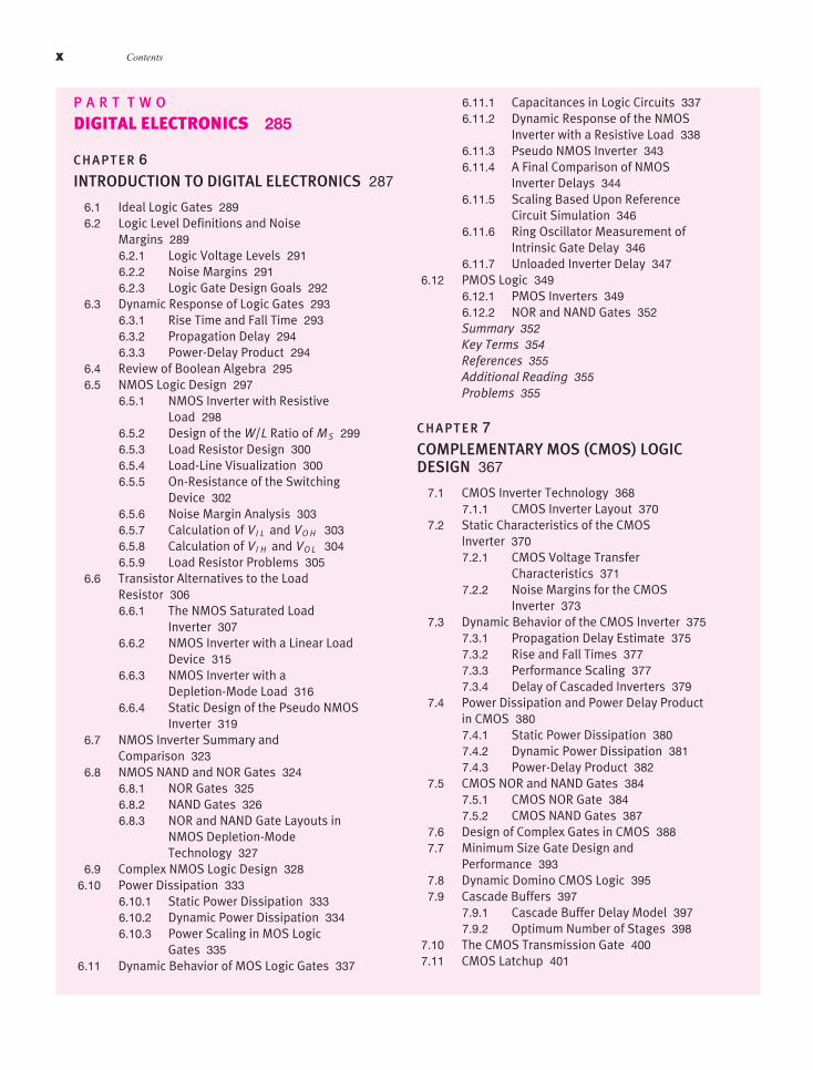
6.1 Ideal Logic Gates 2896.2 Logic Level Definitions and Noise
Margins 2896.2.1 Logic Voltage Levels 2916.2.2 Noise Margins 2916.2.3 Logic Gate Design Goals 292
6.3 Dynamic Response of Logic Gates 2936.3.1 Rise Time and Fall Time 2936.3.2 Propagation Delay 2946.3.3 Power-Delay Product 294
6.4 Review of Boolean Algebra 2956.5 NMOS Logic Design 297
6.5.1 NMOS Inverter with ResistiveLoad 298
6.5.2 Design of the W/L Ratio of MS 2996.5.3 Load Resistor Design 3006.5.4 Load-Line Visualization 3006.5.5 On-Resistance of the Switching
Device 3026.5.6 Noise Margin Analysis 3036.5.7 Calculation of VI L and VO H 3036.5.8 Calculation of VI H and VO L 3046.5.9 Load Resistor Problems 305
6.6 Transistor Alternatives to the LoadResistor 3066.6.1 The NMOS Saturated Load
Inverter 3076.6.2 NMOS Inverter with a Linear Load
Device 3156.6.3 NMOS Inverter with a
Depletion-Mode Load 3166.6.4 Static Design of the Pseudo NMOS
Inverter 3196.7 NMOS Inverter Summary and
Comparison 3236.8 NMOS NAND and NOR Gates 324
6.8.1 NOR Gates 3256.8.2 NAND Gates 3266.8.3 NOR and NAND Gate Layouts in
NMOS Depletion-ModeTechnology 327
6.9 Complex NMOS Logic Design 3286.10 Power Dissipation 333
6.10.1 Static Power Dissipation 3336.10.2 Dynamic Power Dissipation 3346.10.3 Power Scaling in MOS Logic
Gates 3356.11 Dynamic Behavior of MOS Logic Gates 337
6.11.1 Capacitances in Logic Circuits 3376.11.2 Dynamic Response of the NMOS
Inverter with a Resistive Load 3386.11.3 Pseudo NMOS Inverter 3436.11.4 A Final Comparison of NMOS
Inverter Delays 3446.11.5 Scaling Based Upon Reference
Circuit Simulation 3466.11.6 Ring Oscillator Measurement of
Intrinsic Gate Delay 3466.11.7 Unloaded Inverter Delay 347
6.12 PMOS Logic 3496.12.1 PMOS Inverters 3496.12.2 NOR and NAND Gates 352Summary 352Key Terms 354References 355Additional Reading 355Problems 355
CHAPTER 7
COMPLEMENTARY MOS (CMOS) LOGICDESIGN 367
7.1 CMOS Inverter Technology 3687.1.1 CMOS Inverter Layout 370
7.2 Static Characteristics of the CMOSInverter 3707.2.1 CMOS Voltage Transfer
Characteristics 3717.2.2 Noise Margins for the CMOS
Inverter 3737.3 Dynamic Behavior of the CMOS Inverter 375
7.3.1 Propagation Delay Estimate 3757.3.2 Rise and Fall Times 3777.3.3 Performance Scaling 3777.3.4 Delay of Cascaded Inverters 379
7.4 Power Dissipation and Power Delay Productin CMOS 3807.4.1 Static Power Dissipation 3807.4.2 Dynamic Power Dissipation 3817.4.3 Power-Delay Product 382
7.5 CMOS NOR and NAND Gates 3847.5.1 CMOS NOR Gate 3847.5.2 CMOS NAND Gates 387
7.6 Design of Complex Gates in CMOS 3887.7 Minimum Size Gate Design and
Performance 3937.8 Dynamic Domino CMOS Logic 3957.9 Cascade Buffers 397
7.9.1 Cascade Buffer Delay Model 3977.9.2 Optimum Number of Stages 398
7.10 The CMOS Transmission Gate 4007.11 CMOS Latchup 401

Jaeger-1820037 jae80458˙FM˙i-xxvi January 22, 2010 15:50
Contents xi
Summary 404Key Terms 405References 406Problems 406
CHAPTER 8
MOS MEMORY AND STORAGE CIRCUITS 416
8.1 Random Access Memory 4178.1.1 Random Access Memory (RAM)
Architecture 4178.1.2 A 256-Mb Memory Chip 418
8.2 Static Memory Cells 4198.2.1 Memory Cell Isolation and
Access—The 6-T Cell 4228.2.2 The Read Operation 4228.2.3 Writing Data into the 6-T Cell 426
8.3 Dynamic Memory Cells 4288.3.1 The One-Transistor Cell 4308.3.2 Data Storage in the 1-T Cell 4308.3.3 Reading Data from the 1-T Cell 4318.3.4 The Four-Transistor Cell 433
8.4 Sense Amplifiers 4348.4.1 A Sense Amplifier for the 6-T
Cell 4348.4.2 A Sense Amplifier for the 1-T
Cell 4368.4.3 The Boosted Wordline Circuit 4388.4.4 Clocked CMOS Sense
Amplifiers 4388.5 Address Decoders 440
8.5.1 NOR Decoder 4408.5.2 NAND Decoder 4408.5.3 Decoders in Domino CMOS
Logic 4438.5.4 Pass-Transistor Column
Decoder 4438.6 Read-Only Memory (ROM) 4448.7 Flip-Flops 447
8.7.1 RS Flip-Flop 4498.7.2 The D-Latch Using Transmission
Gates 4508.7.3 A Master-Slave D Flip-Flop 450Summary 451Key Terms 452References 452Problems 453
CHAPTER 9
BIPOLAR LOGIC CIRCUITS 460
9.1 The Current Switch (Emitter-CoupledPair) 4619.1.1 Mathematical Model for Static
Behavior of the Current Switch 462
9.1.2 Current Switch Analysis forvI > VREF 463
9.1.3 Current Switch Analysis forvI < VREF 464
9.2 The Emitter-Coupled Logic (ECL) Gate 4649.2.1 ECL Gate with vI = VH 4659.2.2 ECL Gate with vI = VL 4669.2.3 Input Current of the ECL Gate 4669.2.4 ECL Summary 466
9.3 Noise Margin Analysis for the ECL Gate 4679.3.1 VI L , VO H , VI H , and VO L 4679.3.2 Noise Margins 468
9.4 Current Source Implementation 4699.5 The ECL OR-NOR Gate 4719.6 The Emitter Follower 473
9.6.1 Emitter Follower with a LoadResistor 474
9.7 “Emitter Dotting’’ or “Wired-OR’’ Logic 4769.7.1 Parallel Connection of
Emitter-Follower Outputs 4779.7.2 The Wired-OR Logic Function 477
9.8 ECL Power-Delay Characteristics 4779.8.1 Power Dissipation 4779.8.2 Gate Delay 4799.8.3 Power-Delay Product 480
9.9 Current Mode Logic 4819.9.1 CML Logic Gates 4819.9.2 CML Logic Levels 4829.9.3 VE E Supply Voltage 4829.9.4 Higher-Level CML 4839.9.5 CML Power Reduction 4849.9.6 NMOS CML 485
9.10 The Saturating Bipolar Inverter 4879.10.1 Static Inverter Characteristics 4889.10.2 Saturation Voltage of the Bipolar
Transistor 4889.10.3 Load-Line Visualization 4919.10.4 Switching Characteristics of the
Saturated BJT 4919.11 A Transistor-Transistor Logic (TTL)
Prototype 4949.11.1 TTL Inverter for vI = VL 4949.11.2 TTL Inverter for vI = VH 4959.11.3 Power in the Prototype TTL
Gate 4969.11.4 VIH, VIL, and Noise Margins for the
TTL Prototype 4969.11.5 Prototype Inverter Summary 4989.11.6 Fanout Limitations of the TTL
Prototype 4989.12 The Standard 7400 Series TTL Inverter 500
9.12.1 Analysis for vI = VL 5009.12.2 Analysis for vI = VH 501

Jaeger-1820037 jae80458˙FM˙i-xxvi January 22, 2010 15:50
xii Contents
9.12.3 Power Consumption 5039.12.4 TTL Propagation Delay and
Power-Delay Product 5039.12.5 TTL Voltage Transfer Characteristic
and Noise Margins 5039.12.6 Fanout Limitations of Standard
TTL 5049.13 Logic Functions in TTL 504
9.13.1 Multi-Emitter Input Transistors 5059.13.2 TTL NAND Gates 5059.13.3 Input Clamping Diodes 506
9.14 Schottky-Clamped TTL 5069.15 Comparison of the Power-Delay Products of
ECL and TTL 5089.16 BiCMOS Logic 508
9.16.1 BiCMOS Buffers 5099.16.2 BiNMOS Inverters 5119.16.3 BiCMOS Logic Gates 513Summary 513Key Terms 515References 515Additional Reading 515Problems 516
P A R T T H R E E
ANALOG ELECTRONICS 527
CHAPTER 10
ANALOG SYSTEMS AND IDEAL OPERATIONALAMPLIFIERS 529
10.1 An Example of an Analog ElectronicSystem 530
10.2 Amplification 53110.2.1 Voltage Gain 53210.2.2 Current Gain 53310.2.3 Power Gain 53310.2.4 The Decibel Scale 534
10.3 Two-Port Models for Amplifiers 53710.3.1 The g-parameters 537
10.4 Mismatched Source and LoadResistances 541
10.5 Introduction to Operational Amplifiers 54410.5.1 The Differential Amplifier 54410.5.2 Differential Amplifier Voltage
Transfer Characteristic 54510.5.3 Voltage Gain 545
10.6 Distortion in Amplifiers 54810.7 Differential Amplifier Model 54910.8 Ideal Differential and Operational
Amplifiers 55110.8.1 Assumptions for Ideal Operational
Amplifier Analysis 551
10.9 Analysis of Circuits Containing IdealOperational Amplifiers 55210.9.1 The Inverting Amplifier 55310.9.2 The Transresistance Amplifier—A
Current-to-Voltage Converter 55610.9.3 The Noninverting Amplifier 55810.9.4 The Unity-Gain Buffer, or Voltage
Follower 56110.9.5 The Summing Amplifier 56310.9.6 The Difference Amplifier 565
10.10 Frequency-Dependent Feedback 56810.10.1 Bode Plots 56810.10.2 The Low-Pass Amplifier 56810.10.3 The High-Pass Amplifier 57210.10.4 Band-Pass Amplifiers 57510.10.5 An Active Low-Pass Filter 57810.10.6 An Active High-Pass Filter 58110.10.7 The Integrator 58210.10.8 The Differentiator 586Summary 586Key Terms 588References 588Additional Reading 589Problems 589
CHAPTER 11
NONIDEAL OPERATIONAL AMPLIFIERS ANDFEEDBACK AMPLIFIER STABILITY 600
11.1 Classic Feedback Systems 60111.1.1 Closed-Loop Gain Analysis 60211.1.2 Gain Error 602
11.2 Analysis of Circuits Containing NonidealOperational Amplifiers 60311.2.1 Finite Open-Loop Gain 60311.2.2 Nonzero Output Resistance 60611.2.3 Finite Input Resistance 61011.2.4 Summary of Nonideal Inverting and
Noninverting Amplifiers 61411.3 Series and Shunt Feedback Circuits 615
11.3.1 Feedback Amplifier Categories 61511.3.2 Voltage Amplifiers—Series-Shunt
Feedback 61611.3.3 Transimpedance
Amplifiers—Shunt-ShuntFeedback 616
11.3.4 Current Amplifiers—Shunt-SeriesFeedback 616
11.3.5 TransconductanceAmplifiers—Series-SeriesFeedback 616
11.4 Unified Approach to Feedback Amplifier GainCalculation 616

Jaeger-1820037 jae80458˙FM˙i-xxvi January 22, 2010 15:50
Contents xiii
11.4.1 Closed-Loop Gain Analysis 61711.4.2 Resistance Calculation Using
Blackman’S Theorem 61711.5 Series-Shunt Feedback–Voltage
Amplifiers 61711.5.1 Closed-Loop Gain Calculation 61811.5.2 Input Resistance Calculation 61811.5.3 Output Resistance
Calculation 61911.5.4 Series-Shunt Feedback Amplifier
Summary 62011.6 Shunt-Shunt Feedback—Transresistance
Amplifiers 62411.6.1 Closed-Loop Gain Calculation 62511.6.2 Input Resistance Calculation 62511.6.3 Output Resistance Calculation 62511.6.4 Shunt-Shunt Feedback Amplifier
Summary 62611.7 Series-Series Feedback—Transconductance
Amplifiers 62911.7.1 Closed-Loop Gain Calculation 63011.7.2 Input Resistance Calculation 63011.7.3 Output Resistance Calculation 63111.7.4 Series-Series Feedback Amplifier
Summary 63111.8 Shunt-Series Feedback—Current
Amplifiers 63311.8.1 Closed-Loop Gain Calculation 63411.8.2 Input Resistance Calculation 63511.8.3 Output Resistance Calculation 63511.8.4 Series-Series Feedback Amplifier
Summary 63511.9 Finding the Loop Gain Using Successive
Voltage and Current Injection 63811.9.1 Simplifications 641
11.10 Distortion Reduction Through the Use ofFeedback 641
11.11 DC Error Sources and Output RangeLimitations 64211.11.1 Input-Offset Voltage 64311.11.2 Offset-Voltage Adjustment 64411.11.3 Input-Bias and Offset
Currents 64511.11.4 Output Voltage and Current
Limits 64711.12 Common-Mode Rejection and Input
Resistance 65011.12.1 Finite Common-Mode Rejection
Ratio 65011.12.2 Why Is CMRR Important? 65111.12.3 Voltage-Follower Gain Error Due to
CMRR 65411.12.4 Common-Mode Input
Resistance 656
11.12.5 An Alternate Interpretation ofCMRR 657
11.12.6 Power Supply Rejection Ratio 65711.13 Frequency Response and Bandwidth of
Operational Amplifiers 65911.13.1 Frequency Response of the
Noninverting Amplifier 66111.13.2 Inverting Amplifier Frequency
Response 66411.13.3 Using Feedback to Control
Frequency Response 66611.13.4 Large-Signal Limitations—Slew
Rate and Full-PowerBandwidth 668
11.13.5 Macro Model for OperationalAmplifier Frequency Response 669
11.13.6 Complete Op Amp Macro Models inSPICE 670
11.13.7 Examples of CommercialGeneral-Purpose OperationalAmplifiers 670
11.14 Stability of Feedback Amplifiers 67111.14.1 The Nyquist Plot 67111.14.2 First-Order Systems 67211.14.3 Second-Order Systems and Phase
Margin 67311.14.4 Step Response and Phase
Margin 67411.14.5 Third-Order Systems and Gain
Margin 67711.14.6 Determining Stability from the
Bode Plot 678Summary 682Key Terms 684References 684Problems 685
CHAPTER 12
OPERATIONAL AMPLIFIER APPLICATIONS 697
12.1 Cascaded Amplifiers 69812.1.1 Two-Port Representations 69812.1.2 Amplifier Terminology Review 70012.1.3 Frequency Response of Cascaded
Amplifiers 70312.2 The Instrumentation Amplifier 71112.3 Active Filters 714
12.3.1 Low-Pass Filter 71412.3.2 A High-Pass Filter with Gain 71812.3.3 Band-Pass Filter 72012.3.4 The Tow-Thomas Biquad 72212.3.5 Sensitivity 72612.3.6 Magnitude and Frequency
Scaling 727

Jaeger-1820037 jae80458˙FM˙i-xxvi January 22, 2010 15:50
xiv Contents
12.4 Switched-Capacitor Circuits 72812.4.1 A Switched-Capacitor
Integrator 72812.4.2 Noninverting SC Integrator 73012.4.3 Switched-Capacitor Filters 732
12.5 Digital-to-Analog Conversion 73312.5.1 D/A Converter Fundamentals 73312.5.2 D/A Converter Errors 73412.5.3 Digital-to-Analog Converter
Circuits 73712.6 Analog-to-Digital Conversion 740
12.6.1 A/D Converter Fundamentals 74112.6.2 Analog-to-Digital Converter
Errors 74212.6.3 Basic A/D Conversion
Techniques 74312.7 Oscillators 754
12.7.1 The Barkhausen Criteria forOscillation 754
12.7.2 Oscillators EmployingFrequency-Selective RCNetworks 755
12.8 Nonlinear Circuit Applications 76012.8.1 A Precision Half-Wave Rectifier 76012.8.2 Nonsaturating Precision-Rectifier
Circuit 76112.9 Circuits Using Positive Feedback 763
12.9.1 The Comparator and SchmittTrigger 763
12.9.2 The Astable Multivibrator 76512.9.3 The Monostable Multivibrator or
One Shot 766Summary 770Key Terms 772Additional Reading 773Problems 773
CHAPTER 13
SMALL-SIGNAL MODELING AND LINEARAMPLIFICATION 786
13.1 The Transistor as an Amplifier 78713.1.1 The BJT Amplifier 78813.1.2 The MOSFET Amplifier 789
13.2 Coupling and Bypass Capacitors 79013.3 Circuit Analysis Using dc and ac Equivalent
Circuits 79213.3.1 Menu for dc and ac Analysis 792
13.4 Introduction to Small-Signal Modeling 79613.4.1 Graphical Interpretation of the
Small-Signal Behavior of theDiode 796
13.4.2 Small-Signal Modeling of theDiode 797
13.5 Small-Signal Models for Bipolar JunctionTransistors 79913.5.1 The Hybrid-Pi Model 80113.5.2 Graphical Interpretation of the
Transconductance 80213.5.3 Small-Signal Current Gain 80213.5.4 The Intrinsic Voltage Gain of the
BJT 80313.5.5 Equivalent Forms of the
Small-Signal Model 80413.5.6 Simplified Hybrid Pi Model 80513.5.7 Definition of a Small Signal for the
Bipolar Transistor 80513.5.8 Small-Signal Model for the pnp
Transistor 80713.5.9 ac Analysis Versus Transient
Analysis in SPICE 80713.6 The Common-Emitter (C-E) Amplifier 808
13.6.1 Terminal Voltage Gain 80913.6.2 Input Resistance 80913.6.3 Signal Source Voltage Gain 810
13.7 Important Limits and ModelSimplifications 81013.7.1 A Design Guide for the
Common-Emitter Amplifier 81013.7.2 Upper Bound on the
Common-Emitter Gain 81213.7.3 Small-Signal Limit for the
Common-emitter Amplifier 81213.8 Small-Signal Models for Field-Effect
Transistors 81513.8.1 Small-Signal Model for
the MOSFET 81513.8.2 Intrinsic Voltage Gain of
the MOSFET 81713.8.3 Definition of Small-Signal
Operation for the MOSFET 81713.8.4 Body Effect in the Four-Terminal
MOSFET 81813.8.5 Small-Signal Model for the PMOS
Transistor 81913.8.6 Small-Signal Model for the Junction
Field-Effect Transistor 82013.9 Summary and Comparison of the
Small-Signal Models of the BJT and FET 82113.10 The Common-Source Amplifier 824
13.10.1 Common-Source Terminal VoltageGain 825
13.10.2 Signal Source Voltage Gain for theCommon-Source Amplifier 825
13.10.3 A Design Guide for theCommon-Source Amplifier 826
13.10.4 Small-Signal Limit for theCommon-Source Amplifier 827

Jaeger-1820037 jae80458˙FM˙i-xxvi January 22, 2010 15:50
Contents xv
13.10.5 Input Resistances of theCommon-Emitter andCommon-Source Amplifiers 829
13.10.6 Common-Emitter andCommon-Source OutputResistances 832
13.10.7 Comparison of the Three AmplifierResistances 838
13.11 Common-Emitter and Common-SourceAmplifier Summary 83813.11.1 Guidelines for Neglecting the
Transistor OutputResistance 839
13.12 Amplifier Power and Signal Range 83913.12.1 Power Dissipation 83913.12.2 Signal Range 840Summary 843Key Terms 844Problems 845
CHAPTER 14
SINGLE-TRANSISTOR AMPLIFIERS 857
14.1 Amplifier Classification 85814.1.1 Signal Injection and
Extraction—The BJT 85814.1.2 Signal Injection and
Extraction—The FET 85914.1.3 Common-Emitter (C-E) and
Common-Source (C-S)Amplifiers 860
14.1.4 Common-Collector (C-C) andCommon-Drain (C-D)Topologies 861
14.1.5 Common-Base (C-B) andCommon-Gate (C-G) Amplifiers 863
14.1.6 Small-Signal Model Review 86414.2 Inverting Amplifiers—Common-Emitter and
Common-Source Circuits 86414.2.1 The Common-Emitter (C-E)
Amplifier 86414.2.2 Common-Emitter Example
Comparison 87714.2.3 The Common-Source Amplifier 87714.2.4 Small-Signal Limit for the
Common-Source Amplifier 88014.2.5 Common-Emitter and
Common-Source AmplifierCharacteristics 884
14.2.6 C-E/C-S Amplifier Summary 88514.2.7 Equivalent Transistor
Representation of the GeneralizedC-E/C-S Transistor 885
14.3 Follower Circuits—Common-Collector andCommon-Drain Amplifiers 88614.3.1 Terminal Voltage Gain 88614.3.2 Input Resistance 88714.3.3 Signal Source Voltage Gain 88814.3.4 Follower Signal Range 88814.3.5 Follower Output Resistance 88914.3.6 Current Gain 89014.3.7 C-C/C-D Amplifier Summary 890
14.4 Noninverting Amplifiers—Common-Baseand Common-Gate Circuits 89414.4.1 Terminal Voltage Gain and Input
Resistance 89514.4.2 Signal Source Voltage Gain 89614.4.3 Input Signal Range 89714.4.4 Resistance at the Collector and
Drain Terminals 89714.4.5 Current Gain 89814.4.6 Overall Input and Output
Resistances for the NoninvertingAmplifiers 899
14.4.7 C-B/C-G Amplifier Summary 90214.5 Amplifier Prototype Review and
Comparison 90314.5.1 The BJT Amplifiers 90314.5.2 The FET Amplifiers 905
14.6 Common-Source Amplifiers Using MOSInverters 90714.6.1 Voltage Gain Estimate 90814.6.2 Detailed Analysis 90914.6.3 Alternative Loads 91014.6.4 Input and Output Resistances 911
14.7 Coupling and Bypass Capacitor Design 91414.7.1 Common-Emitter and
Common-Source Amplifiers 91414.7.2 Common-Collector and
Common-Drain Amplifiers 91914.7.3 Common-Base and Common-Gate
Amplifiers 92114.7.4 Setting Lower Cutoff Frequency
fL 92414.8 Amplifier Design Examples 925
14.8.1 Monte Carlo Evaluation of theCommon-Base AmplifierDesign 934
14.9 Multistage ac-Coupled Amplifiers 93914.9.1 A Three-Stage ac-Coupled
Amplifier 93914.9.2 Voltage Gain 94114.9.3 Input Resistance 94314.9.4 Signal Source Voltage Gain 94314.9.5 Output Resistance 94314.9.6 Current and Power Gain 944

Jaeger-1820037 jae80458˙FM˙i-xxvi January 22, 2010 15:50
xvi Contents
14.9.7 Input Signal Range 94514.9.8 Estimating the Lower Cutoff
Frequency of the MultistageAmplifier 948
Summary 950Key Terms 951Additional Reading 952Problems 952
CHAPTER 15
DIFFERENTIAL AMPLIFIERS AND OPERATIONALAMPLIFIER DESIGN 968
15.1 Differential Amplifiers 96915.1.1 Bipolar and MOS Differential
Amplifiers 96915.1.2 dc Analysis of the Bipolar
Differential Amplifier 97015.1.3 Transfer Characteristic for the
Bipolar DifferentialAmplifier 972
15.1.4 ac Analysis of the BipolarDifferential Amplifier 973
15.1.5 Differential-Mode Gain and Inputand Output Resistances 974
15.1.6 Common-Mode Gain and InputResistance 976
15.1.7 Common-Mode Rejection Ratio(CMRR) 978
15.1.8 Analysis Using Differential- andCommon-Mode Half-Circuits 979
15.1.9 Biasing with Electronic CurrentSources 982
15.1.10 Modeling the Electronic CurrentSource in SPICE 983
15.1.11 dc Analysis of the MOSFETDifferential Amplifier 983
15.1.12 Differential-Mode InputSignals 985
15.1.13 Small-Signal TransferCharacteristic for the MOSDifferential Amplifier 986
15.1.14 Common-Mode Input Signals 98615.1.15 Two-Port Model for Differential
Pairs 98715.2 Evolution to Basic Operational
Amplifiers 99115.2.1 A Two-Stage Prototype for an
Operational Amplifier 99215.2.2 Improving the Op Amp Voltage
Gain 99715.2.3 Output Resistance Reduction 99815.2.4 A CMOS Operational Amplifier
Prototype 1002
15.2.5 BiCMOS Amplifiers 100415.2.6 All Transistor
Implementations 100415.3 Output Stages 1006
15.3.1 The Source Follower—A Class-AOutput Stage 1006
15.3.2 Efficiency of Class-AAmplifiers 1007
15.3.3 Class-B Push-Pull OutputStage 1008
15.3.4 Class-AB Amplifiers 101015.3.5 Class-AB Output Stages for
Operational Amplifiers 101115.3.6 Short-Circuit Protection 101115.3.7 Transformer Coupling 1013
15.4 Electronic Current Sources 101615.4.1 Single-Transistor Current
Sources 101715.4.2 Figure of Merit for Current
Sources 101715.4.3 Higher Output Resistance
Sources 101815.4.4 Current Source Design
Examples 1018Summary 1027Key Terms 1028References 1029Additional Reading 1029Problems 1029
CHAPTER 16
ANALOG INTEGRATED CIRCUIT DESIGNTECHNIQUES 1046
16.1 Circuit Element Matching 104716.2 Current Mirrors 1049
16.2.1 dc Analysis of the MOS TransistorCurrent Mirror 1049
16.2.2 Changing the MOS MirrorRatio 1051
16.2.3 dc Analysis of the BipolarTransistor Current Mirror 1052
16.2.4 Altering the BJT Current MirrorRatio 1054
16.2.5 Multiple Current Sources 105516.2.6 Buffered Current Mirror 105616.2.7 Output Resistance of the Current
Mirrors 105716.2.8 Two-Port Model for the Current
Mirror 105816.2.9 The Widlar Current Source 106016.2.10 The MOS Version of the Widlar
Source 1063
Jaeger-1820037 jae80458˙FM˙i-xxvi January 22, 2010 15:50
Contents xvii
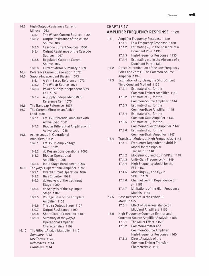
16.3 High-Output-Resistance CurrentMirrors 106316.3.1 The Wilson Current Sources 106416.3.2 Output Resistance of the Wilson
Source 106516.3.3 Cascode Current Sources 106616.3.4 Output Resistance of the Cascode
Sources 106716.3.5 Regulated Cascode Current
Source 106816.3.6 Current Mirror Summary 1069
16.4 Reference Current Generation 107216.5 Supply-Independent Biasing 1073
16.5.1 A VB E -Based Reference 107316.5.2 The Widlar Source 107316.5.3 Power-Supply-Independent Bias
Cell 107416.5.4 A Supply-Independent MOS
Reference Cell 107516.6 The Bandgap Reference 107716.7 The Current Mirror As an Active
Load 108116.7.1 CMOS Differential Amplifier with
Active Load 108116.7.2 Bipolar Differential Amplifier with
Active Load 108816.8 Active Loads in Operational
Amplifiers 109216.8.1 CMOS Op Amp Voltage
Gain 109216.8.2 dc Design Considerations 109316.8.3 Bipolar Operational
Amplifiers 109516.8.4 Input Stage Breakdown 1096
16.9 The �A741 Operational Amplifier 109716.9.1 Overall Circuit Operation 109716.9.2 Bias Circuitry 109816.9.3 dc Analysis of the 741 Input
Stage 109916.9.4 ac Analysis of the 741 Input
Stage 110216.9.5 Voltage Gain of the Complete
Amplifier 110316.9.6 The 741 Output Stage 110716.9.7 Output Resistance 110916.9.8 Short Circuit Protection 110916.9.9 Summary of the �A741
Operational AmplifierCharacteristics 1109
16.10 The Gilbert Analog Multiplier 1110Summary 1112Key Terms 1113References 1114Problems 1114
CHAPTER 17
AMPLIFIER FREQUENCY RESPONSE 1128
17.1 Amplifier Frequency Response 112917.1.1 Low-Frequency Response 113017.1.2 Estimating ωL in the Absence of a
Dominant Pole 113017.1.3 High-Frequency Response 113317.1.4 Estimating ωH in the Absence of a
Dominant Pole 113317.2 Direct Determination of the Low-Frequency
Poles and Zeros—The Common-SourceAmplifier 1134
17.3 Estimation of ωL Using the Short-CircuitTime-Constant Method 113917.3.1 Estimate of ωL for the
Common-Emitter Amplifier 114017.3.2 Estimate of ωL for the
Common-Source Amplifier 114417.3.3 Estimate of ωL for the
Common-Base Amplifier 114517.3.4 Estimate of ωL for the
Common-Gate Amplifier 114617.3.5 Estimate of ωL for the
Common-Collector Amplifier 114717.3.6 Estimate of ωL for the
Common-Drain Amplifier 114717.4 Transistor Models at High Frequencies 1148
17.4.1 Frequency-Dependent Hybrid-PiModel for the BipolarTransistor 1148
17.4.2 Modeling C π and Cμ in SPICE 114917.4.3 Unity-Gain Frequency fT 114917.4.4 High-Frequency Model for the
FET 115217.4.5 Modeling CGS and CGD in
SPICE 115317.4.6 Channel Length Dependence of
fT 115317.4.7 Limitations of the High-Frequency
Models 115517.5 Base Resistance in the Hybrid-Pi
Model 115517.5.1 Effect of Base Resistance on
Midband Amplifiers 115617.6 High-Frequency Common-Emitter and
Common-Source Amplifier Analysis 115817.6.1 The Miller Effect 115917.6.2 Common-Emitter and
Common-Source AmplifierHigh-Frequency Response 1160
17.6.3 Direct Analysis of theCommon-Emitter TransferCharacteristic 1162

Jaeger-1820037 jae80458˙FM˙i-xxvi January 22, 2010 15:50
xviii Contents
17.6.4 Poles of the Common-EmitterAmplifier 1163
17.6.5 Dominant Pole for theCommon-Source Amplifier 1166
17.6.6 Estimation of ωH Using theOpen-Circuit Time-ConstantMethod 1167
17.6.7 Common-Source Amplifier withSource DegenerationResistance 1170
17.6.8 Poles of the Common-Emitter withEmitter DegenerationResistance 1172
17.7 Common-Base and Common-GateAmplifier High-Frequency Response 1174
17.8 Common-Collector and Common-DrainAmplifier High-Frequency Response 1177
17.9 Single-Stage Amplifier High-FrequencyResponse Summary 117917.9.1 Amplifier Gain-Bandwidth
Limitations 118017.10 Frequency Response of Multistage
Amplifiers 118117.10.1 Differential Amplifier 118117.10.2 The Common-Collector/
Common-Base Cascade 118217.10.3 High-Frequency Response of the
Cascode Amplifier 118417.10.4 Cutoff Frequency for the Current
Mirror 118517.10.5 Three-Stage Amplifier
Example 118717.11 Introduction to Radio Frequency
Circuits 119317.11.1 Radio Frequency Amplifiers 119417.11.2 The Shunt-Peaked Amplifier 119417.11.3 Single-Tuned Amplifier 119717.11.4 Use of a Tapped Inductor—The
Auto Transformer 119917.11.5 Multiple Tuned
Circuits—Synchronous andStagger Tuning 1201
17.11.6 Common-Source Amplifier withInductive Degeneration 1202
17.12 Mixers and Balanced Modulators 120517.12.1 Introduction to Mixer
Operation 120517.12.2 A Single-Balanced Mixer 120617.12.3 The Differential Pair as a
Single-Balanced Mixer 120717.12.4 A Double-Balanced Mixer 120817.12.5 The Gilbert Multiplier as a
Double-BalancedMixer/Modulator 1210
Summary 1213Key Terms 1215Reference 1215Problems 1215
CHAPTER 18
TRANSISTOR FEEDBACK AMPLIFIERSAND OSCILLATORS 1228
18.1 Basic Feedback System Review 122918.1.1 Closed-Loop Gain 122918.1.2 Closed-Loop Impedances 123018.1.3 Feedback Effects 1230
18.2 Feedback Amplifier Analysis atMidband 1232
18.3 Feedback Amplifier Circuit Examples 123418.3.1 Series-Shunt Feedback—Voltage
Amplifiers 123418.3.2 Differential Input Series-Shunt
Voltage Amplifier 123918.3.3 Shunt-Shunt
Feedback—TransresistanceAmplifiers 1242
18.3.4 Series-SeriesFeedback—TransconductanceAmplifiers 1248
18.3.5 Shunt-Series Feedback—CurrentAmplifiers 1251
18.4 Review of Feedback Amplifier Stability 125418.4.1 Closed-Loop Response of the
Uncompensated Amplifier 125418.4.2 Phase Margin 125618.4.3 Higher-Order Effects 125918.4.4 Response of the Compensated
Amplifier 126018.4.5 Small-Signal Limitations 1262
18.5 Single-Pole Operational AmplifierCompensation 126218.5.1 Three-Stage Op Amp Analysis 126318.5.2 Transmission Zeros in FET Op
Amps 126518.5.3 Bipolar Amplifier
Compensation 126618.5.4 Slew Rate of the Operational
Amplifier 126618.5.5 Relationships Between Slew Rate
and Gain-Bandwidth Product 126818.6 High-Frequency Oscillators 1277
18.6.1 The Colpitts Oscillator 127818.6.2 The Hartley Oscillator 127918.6.3 Amplitude Stabilization in LC
Oscillators 128018.6.4 Negative Resistance in
Oscillators 1280

Jaeger-1820037 jae80458˙FM˙i-xxvi January 22, 2010 15:50
Contents xix
18.6.5 Negative GM Oscillator 128118.6.6 Crystal Oscillators 1283Summary 1287Key Terms 1289References 1289Problems 1289
A P P E N D I X E S
A Standard Discrete Component Values 1300B Solid-State Device Models and SPICE
Simulation Parameters 1303C Two-Port Review 1310
Index 1313

Jaeger-1820037 jae80458˙FM˙i-xxvi January 22, 2010 15:50
PREFACE
Through study of this text, the reader will develop a com-prehensive understanding of the basic techniques of mod-ern electronic circuit design, analog and digital, discreteand integrated. Even though most readers may not ulti-mately be engaged in the design of integrated circuits (ICs)themselves, a thorough understanding of the internal circuitstructure of ICs is prerequisite to avoiding many pitfalls thatprevent the effective and reliable application of integratedcircuits in system design.
Digital electronics has evolved to be an extremely im-portant area of circuit design, but it is included almost asan afterthought in many introductory electronics texts. Wepresent a more balanced coverage of analog and digital cir-cuits. The writing integrates the authors’ extensive indus-trial backgrounds in precision analog and digital design withtheir many years of experience in the classroom. A broadspectrum of topics is included, and material can easily beselected to satisfy either a two-semester or three-quartersequence in electronics.
IN THIS EDITIONThis edition continues to update the material to achieveimproved readability and accessibility to the student. Inaddition to general material updates, a number of spe-cific changes have been included in Parts I and II, Solid-State Electronics and Devices and Digital Electronics,respectively. A new closed-form solution to four-resistorMOSFET biasing is introduced as well as an improvediterative strategy for diode Q-point analysis. JFET devicesare important in analog design and have been reintro-duced at the end of Chapter 4. Simulation-based logic gatescaling is introduced in the MOS logic chapters, and anenhanced discussion of noise margin is included as a newElectronics-in-Action (EIA) feature. Current-mode logic(CML) is heavily used in high performance SiGe ICs, anda CML section is added to the Bipolar Logic chapter.
This revision contains major reorganization and revi-sion of the analog portion (Part III) of the text. The introduc-tory amplifier material (old Chapter 10) is now introduced
in a “just-in-time” basis in the three op-amp chapters. Spe-cific sections have been added with qualitative descriptionsof the operation of basic op-amp circuits and each transistoramplifier configuration as well as the transistors themselves.
Feedback analysis using two-ports has been eliminatedfrom Chapter 18 in favor of a consistent loop-gain analy-sis approach to all feedback configurations that begins inthe op-amp chapters. The important successive voltage andcurrent injection technique for finding loop-gain is now in-cluded in Chapter 11, and Blackman’s theorem is utilized tofind input and output resistances of closed-loop amplifiers.SPICE examples have been modified to utilize three- andfive-terminal built-in op-amp models.
Chapter 10, Analog Systems and Ideal OperationalAmplifiers, provides an introduction to amplifiers and cov-ers the basic ideal op-amp circuits.
Chapter 11, Characteristics and Limitations of Opera-tional Amplifiers, covers the limitations of nonideal op ampsincluding frequency response and stability and the four clas-sic feedback circuits including series-shunt, shunt-shunt,shunt-series and series-series feedback amplifiers.
Chapter 12, Operational Amplifier Applications, col-lects together all the op-amp applications including multi-stage amplifiers, filters, A/D and D/A converters, sinusoidaloscillators, and multivibrators.
Redundant material in transistor amplifier chapters 13and 14 has been merged or eliminated wherever possible.Other additions to the analog material include discussion ofrelations between MOS logic inverters and common-sourceamplifiers, distortion reduction through feedback, the rela-tionship between step response and phase margin, NMOSdifferential amplifiers with NMOS load transistors, the reg-ulated cascode current source, and the Gilbert multiplier.
Because of the renaissance and pervasive use of RFcircuits, the introductory section on RF amplifiers, now inChapter 17, has been expanded to include shunt-peakedand tuned amplifiers, and the use of inductive degenerationin common-source amplifiers. New material on mixers in-cludes passive, active, single- and double-balanced mixersand the widely used Gilbert mixer.
xx

Jaeger-1820037 jae80458˙FM˙i-xxvi January 22, 2010 15:50
Preface xxi
Chapter 18, Transistor Feedback Amplifiers andOscillators, presents examples of transistor feedback am-plifiers and transistor oscillator implementations. The tran-sistor oscillator section has been expanded to include adiscussion of negative resistance in oscillators and thenegative Gm oscillator cell.
Several other important enhancements include:
• SPICE support on the web now includesexamples in NI Multisim™ software inaddition to PSpice® .
• At least 35 percent revised or new problems.• New PowerPoint® slides are available from
McGraw-Hill.• A group of tested design problems are also
available.
The Structured Problem Solving Approach continues to beutilized throughout the examples. We continue to expand thepopular Electronics-in-Action Features with the addition ofDiode Rectifier as an AM Demodulator; High PerformanceCMOS Technologies; A Second Look at Noise Margins(graphical flip-flop approach); Offset Voltage, Bias Cur-rent and CMRR Measurement; Sample-and-Hold Circuits;Voltage Regulator with Series Pass Transistor; Noise Fac-tor, Noise Figure and Minimum Detectable Signal; Series-Parallel and Parallel-Series Network Transformations; andPassive Diode Ring Mixer.
Chapter Openers enhance the readers understanding ofhistorical developments in electronics. Design notes high-light important ideas that the circuit designer should re-member. The World Wide Web is viewed as an integralextension of the text, and a wide range of supporting mate-rials and resource links are maintained and updated on theMcGraw-Hill website (www.mhhe.com/jaeger).
Features of the book are outlined below.
The Structured Problem-Solving Approach is usedthroughout the examples.
Electronics-in-Action features in each chapter.
Chapter openers highlighting developments in thefield of electronics.
Design Notes and emphasis on practical circuitdesign.
Broad use of SPICE throughout the text andexamples.
Integrated treatment of device modeling in SPICE.
Numerous Exercises, Examples, and DesignExamples.
Large number of new problems.
Integrated web materials.
Continuously updated web resources and links.
Placing the digital portion of the book first is also bene-ficial to students outside of electrical engineering, partic-ularly computer engineering or computer science majors,who may only take the first course in a sequence of elec-tronics courses.
The material in Part II deals primarily with the internaldesign of logic gates and storage elements. A comprehen-sive discussion of NMOS and CMOS logic design is pre-sented in Chapters 6 and 7, and a discussion of memorycells and peripheral circuits appears in Chapter 8. Chap-ter 9 on bipolar logic design includes discussion of ECL,CML and TTL. However, the material on bipolar logic hasbeen reduced in deference to the import of MOS technol-ogy. This text does not include any substantial design atthe logic block level, a topic that is fully covered in digitaldesign courses.
Parts I and II of the text deal only with the large-signalcharacteristics of the transistors. This allows readers to be-come comfortable with device behavior and i-v characteris-tics before they have to grasp the concept of splitting circuitsinto different pieces (and possibly different topologies) toperform dc and ac small-signal analyses. (The concept of asmall-signal is formally introduced in Part III, Chapter 13.)
Although the treatment of digital circuits is more ex-tensive than most texts, more than 50 percent of the mate-rial in the book, Part III, still deals with traditional analogcircuits. The analog section begins in Chapter 10 with adiscussion of amplifier concepts and classic ideal op-ampcircuits. Chapter 11 presents a detailed discussion of non-ideal op amps, and Chapter 12 presents a range of op-ampapplications. Chapter 13 presents a comprehensive devel-opment of the small-signal models for the diode, BJT, andFET. The hybrid-pi model and pi-models for the BJT andFET are used throughout.
Chapter 14 provides in-depth discussion of single-stage amplifier design and multistage ac coupled amplifiers.Coupling and bypass capacitor design is also covered inChapter 14. Chapter 15 discusses dc coupled multistageamplifiers and introduces prototypical op amp circuits.Chapter 16 continues with techniques that are important inIC design and studies the classic 741 operational amplifier.
Chapter 17 develops the high-frequency models for thetransistors and presents a detailed discussion of analysis ofhigh-frequency circuit behavior. The final chapter presentsexamples of transistor feedback amplifiers. Discussion offeedback amplifier stability and oscillators conclude thetext.
Jaeger-1820037 jae80458˙FM˙i-xxvi January 22, 2010 15:50
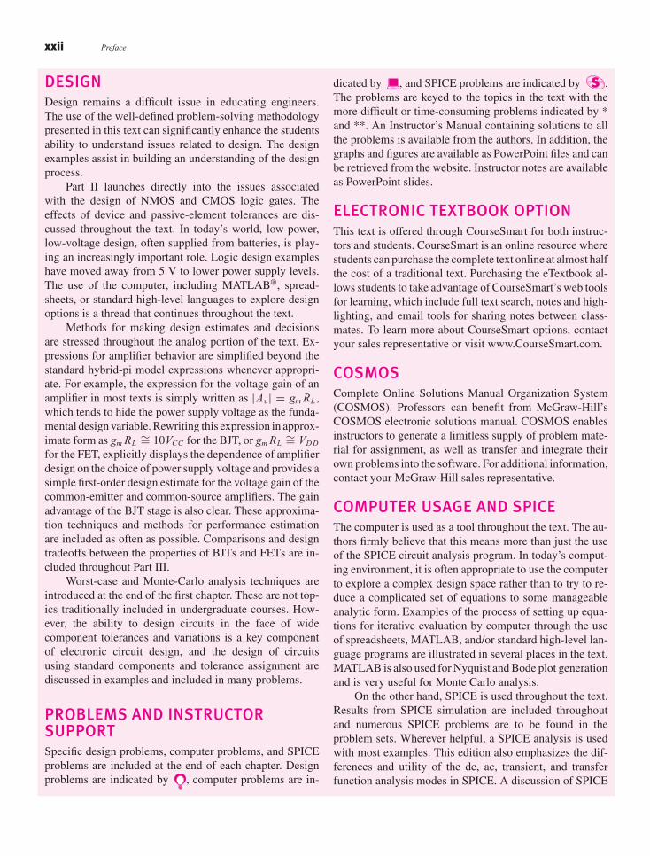
xxii Preface
DESIGNDesign remains a difficult issue in educating engineers.The use of the well-defined problem-solving methodologypresented in this text can significantly enhance the studentsability to understand issues related to design. The designexamples assist in building an understanding of the designprocess.
Part II launches directly into the issues associatedwith the design of NMOS and CMOS logic gates. Theeffects of device and passive-element tolerances are dis-cussed throughout the text. In today’s world, low-power,low-voltage design, often supplied from batteries, is play-ing an increasingly important role. Logic design exampleshave moved away from 5 V to lower power supply levels.The use of the computer, including MATLAB® , spread-sheets, or standard high-level languages to explore designoptions is a thread that continues throughout the text.
Methods for making design estimates and decisionsare stressed throughout the analog portion of the text. Ex-pressions for amplifier behavior are simplified beyond thestandard hybrid-pi model expressions whenever appropri-ate. For example, the expression for the voltage gain of anamplifier in most texts is simply written as |Av| = gm RL ,which tends to hide the power supply voltage as the funda-mental design variable. Rewriting this expression in approx-imate form as gm RL
∼= 10VCC for the BJT, or gm RL∼= VDD
for the FET, explicitly displays the dependence of amplifierdesign on the choice of power supply voltage and provides asimple first-order design estimate for the voltage gain of thecommon-emitter and common-source amplifiers. The gainadvantage of the BJT stage is also clear. These approxima-tion techniques and methods for performance estimationare included as often as possible. Comparisons and designtradeoffs between the properties of BJTs and FETs are in-cluded throughout Part III.
Worst-case and Monte-Carlo analysis techniques areintroduced at the end of the first chapter. These are not top-ics traditionally included in undergraduate courses. How-ever, the ability to design circuits in the face of widecomponent tolerances and variations is a key componentof electronic circuit design, and the design of circuitsusing standard components and tolerance assignment arediscussed in examples and included in many problems.
PROBLEMS AND INSTRUCTORSUPPORTSpecific design problems, computer problems, and SPICEproblems are included at the end of each chapter. Designproblems are indicated by , computer problems are in-
dicated by , and SPICE problems are indicated by .The problems are keyed to the topics in the text with themore difficult or time-consuming problems indicated by *and **. An Instructor’s Manual containing solutions to allthe problems is available from the authors. In addition, thegraphs and figures are available as PowerPoint files and canbe retrieved from the website. Instructor notes are availableas PowerPoint slides.
ELECTRONIC TEXTBOOK OPTIONThis text is offered through CourseSmart for both instruc-tors and students. CourseSmart is an online resource wherestudents can purchase the complete text online at almost halfthe cost of a traditional text. Purchasing the eTextbook al-lows students to take advantage of CourseSmart’s web toolsfor learning, which include full text search, notes and high-lighting, and email tools for sharing notes between class-mates. To learn more about CourseSmart options, contactyour sales representative or visit www.CourseSmart.com.
COSMOSComplete Online Solutions Manual Organization System(COSMOS). Professors can benefit from McGraw-Hill’sCOSMOS electronic solutions manual. COSMOS enablesinstructors to generate a limitless supply of problem mate-rial for assignment, as well as transfer and integrate theirown problems into the software. For additional information,contact your McGraw-Hill sales representative.
COMPUTER USAGE AND SPICEThe computer is used as a tool throughout the text. The au-thors firmly believe that this means more than just the useof the SPICE circuit analysis program. In today’s comput-ing environment, it is often appropriate to use the computerto explore a complex design space rather than to try to re-duce a complicated set of equations to some manageableanalytic form. Examples of the process of setting up equa-tions for iterative evaluation by computer through the useof spreadsheets, MATLAB, and/or standard high-level lan-guage programs are illustrated in several places in the text.MATLAB is also used for Nyquist and Bode plot generationand is very useful for Monte Carlo analysis.
On the other hand, SPICE is used throughout the text.Results from SPICE simulation are included throughoutand numerous SPICE problems are to be found in theproblem sets. Wherever helpful, a SPICE analysis is usedwith most examples. This edition also emphasizes the dif-ferences and utility of the dc, ac, transient, and transferfunction analysis modes in SPICE. A discussion of SPICE

Jaeger-1820037 jae80458˙FM˙i-xxvi January 22, 2010 15:50
Preface xxiii
device modeling is included following the introductionto each semiconductor device, and typical SPICE modelparameters are presented with the models.
ACKNOWLEDGMENTSWe want to thank the large number of people who have hadan impact on the material in this text and on its prepara-tion. Our students have helped immensely in polishing themanuscript and have managed to survive the many revi-sions of the manuscript. Our department heads, J. D. Irwinof Auburn University and L. R. Harriott of the Universityof Virginia, have always been highly supportive of facultyefforts to develop improved texts.
We want to thank all the reviewers and survey respon-dents including
Vijay K. AroraWilkes University
Kurt BehpourCalifornia Polytechnic
State University,San Luis Obispo
David A. BorkholderRochester Institute of
Technology
Dmitri DonetskiStony Brook University
Ethan FarquharThe University of Tennessee,
Knoxville
Melinda HoltzmanPortland State University
Anthony JohnsonThe University of Toledo
Marian K. KazimierczukWright State University
G. Roientan LahijiProfessor, Iran University
of Science andTechnology
Adjunct Professor,University of Michigan
Stanislaw F. LegowskiUniversity of Wyoming
Milica MarkovicCalifornia State University
Sacramento
James E. MorrisPortland State University
Maryam MoussaviCalifornia State University
Long Beach
Kenneth V. NorenUniversity of Idaho
John OrtizUniversity of Texas at
San Antonio
We are also thankful for inspiration from the classictext Applied Electronics by J. F. Pierce and T. J. Paulus.Professor Blalock learned electronics from Professor Piercemany years ago and still appreciates many of the analyticaltechniques employed in their long out-of-print text.
We would like to thank Gabriel Chindris of TechnicalUniversity of Cluj-Napoca in Romania for his assistance increating the simulations for the NI MultisimTM examples.
Finally, we want to thank the team at McGraw-Hill including Raghothaman Srinivasan, Global Publisher;Darlene Schueller, Developmental Editor; Curt Reynolds,Senior Marketing Manager; Jane Mohr, Senior Project Man-ager; Brenda Rolwes, Design Coordinator; John Leland andLouAnn Wilson, Photo Research Coordinators; Kara Ku-dronowicz, Senior Production Supervisor; Sandy Schnee,Senior Media Project Manager; and Dheeraj Chahal, FullService Project Manager, MPS Limited.
In developing this text, we have attempted to integrateour industrial backgrounds in precision analog and digitaldesign with many years of experience in the classroom. Wehope we have at least succeeded to some extent. Construc-tive suggestions and comments will be appreciated.
Richard C. Jaeger
Auburn University
Travis N. Blalock
University of Virginia

Jaeger-1820037 jae80458˙FM˙i-xxvi January 22, 2010 15:50
CHAPTER-BY-CHAPTER SUMMARY
PART I—SOLID-STATE ELECTRONICSAND DEVICESChapter 1 provides a historical perspective on the field ofelectronics beginning with vacuum tubes and advancing togiga-scale integration and its impact on the global economy.Chapter 1 also provides a classification of electronic signalsand a review of some important tools from network anal-ysis, including a review of the ideal operational amplifier.Because developing a good problem-solving methodologyis of such import to an engineer’s career, the comprehen-sive Structured Problem Solving Approach is used to helpthe students develop their problem solving skills. The struc-tured approach is discussed in detail in the first chapter andused in all the subsequent examples in the text. Componenttolerances and variations play an extremely important rolein practical circuit design, and Chapter 1 closes with intro-ductions to tolerances, temperature coefficients, worst-casedesign, and Monte Carlo analysis.
Chapter 2 deviates from the recent norm and discussessemiconductor materials including the covalent-bond andenergy-band models of semiconductors. The chapter in-cludes material on intrinsic carrier density, electron and holepopulations, n- and p-type material, and impurity doping.Mobility, resistivity, and carrier transport by both drift anddiffusion are included as topics. Velocity saturation is dis-cussed, and an introductory discussion of microelectronicfabrication has been merged with Chapter 2.
Chapter 3 introduces the structure and i-v character-istics of solid-state diodes. Discussions of Schottky diodes,variable capacitance diodes, photo-diodes, solar cells, andLEDs are also included. This chapter introduces the con-cepts of device modeling and the use of different levelsof modeling to achieve various approximations to reality.The SPICE model for the diode is discussed. The con-cepts of bias, operating point, and load-line are all intro-duced, and iterative mathematical solutions are also used tofind the operating point with MATLAB and spreadsheets.Diode applications in rectifiers are discussed in detail and a
discussion of the dynamic switching characteristics ofdiodes is also presented.
Chapter 4 discusses MOS and junction field-effecttransistors, starting with a qualitative description of theMOS capacitor. Models are developed for the FET i-v char-acteristics, and a complete discussion of the regions of op-eration of the device is presented. Body effect is included.MOS transistor performance limits including scaling, cut-off frequency, and subthreshold conduction are discussed aswell as basic �-based layout methods. Biasing circuits andload-line analysis are presented. The FET SPICE modelsand model parameters are discussed in Chapter 4.
Chapter 5 introduces the bipolar junction transistorand presents a heuristic development of the Transport (sim-plified Gummel-Poon) model of the BJT based upon su-perposition. The various regions of operation are discussedin detail. Common-emitter and common-base current gainsare defined, and base transit-time, diffusion capacitance andcutoff frequency are all discussed. Bipolar technology andphysical structure are introduced. The four-resistor bias cir-cuit is discussed in detail. The SPICE model for the BJT andthe SPICE model parameters are discussed in Chapter 5.
PART II—DIGITAL ELECTRONICSChapter 6 begins with a compact introduction to digitalelectronics. Terminology discussed includes logic levels,noise margins, rise-and-fall times, propagation delay, fanout, fan in, and power-delay product. A short review ofBoolean algebra is included. The introduction to MOS logicdesign is now merged with Chapter 6 and follows the histor-ical evolution of NMOS logic gates focusing on the designof saturated-load, and depletion-load circuit families. Theimpact of body effect on MOS logic circuit design is dis-cussed in detail. The concept of reference inverter scalingis developed and employed to affect the design of other in-verters, NAND gates, NOR gates, and complex logic func-tions throughout Chapters 6 and 7. Capacitances in MOS
xxiv
Jaeger-1820037 jae80458˙FM˙i-xxvi January 22, 2010 15:50
Chapter-by-Chapter Summary xxv
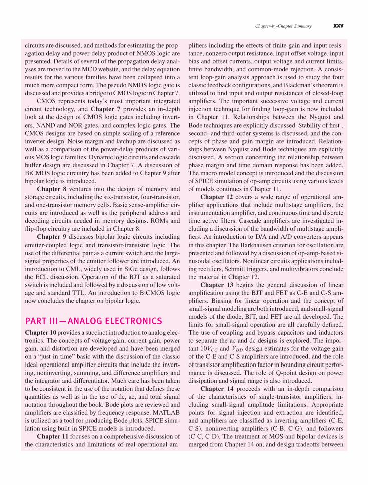
circuits are discussed, and methods for estimating the prop-agation delay and power-delay product of NMOS logic arepresented. Details of several of the propagation delay anal-yses are moved to the MCD website, and the delay equationresults for the various families have been collapsed into amuch more compact form. The pseudo NMOS logic gate isdiscussed and provides a bridge to CMOS logic in Chapter 7.
CMOS represents today’s most important integratedcircuit technology, and Chapter 7 provides an in-depthlook at the design of CMOS logic gates including invert-ers, NAND and NOR gates, and complex logic gates. TheCMOS designs are based on simple scaling of a referenceinverter design. Noise margin and latchup are discussed aswell as a comparison of the power-delay products of vari-ous MOS logic families. Dynamic logic circuits and cascadebuffer design are discussed in Chapter 7. A discussion ofBiCMOS logic circuitry has been added to Chapter 9 afterbipolar logic is introduced.
Chapter 8 ventures into the design of memory andstorage circuits, including the six-transistor, four-transistor,and one-transistor memory cells. Basic sense-amplifier cir-cuits are introduced as well as the peripheral address anddecoding circuits needed in memory designs. ROMs andflip-flop circuitry are included in Chapter 8.
Chapter 9 discusses bipolar logic circuits includingemitter-coupled logic and transistor-transistor logic. Theuse of the differential pair as a current switch and the large-signal properties of the emitter follower are introduced. Anintroduction to CML, widely used in SiGe design, followsthe ECL discussion. Operation of the BJT as a saturatedswitch is included and followed by a discussion of low volt-age and standard TTL. An introduction to BiCMOS logicnow concludes the chapter on bipolar logic.
PART III—ANALOG ELECTRONICSChapter 10 provides a succinct introduction to analog elec-tronics. The concepts of voltage gain, current gain, powergain, and distortion are developed and have been mergedon a “just-in-time” basic with the discussion of the classicideal operational amplifier circuits that include the invert-ing, noninverting, summing, and difference amplifiers andthe integrator and differentiator. Much care has been takento be consistent in the use of the notation that defines thesequantities as well as in the use of dc, ac, and total signalnotation throughout the book. Bode plots are reviewed andamplifiers are classified by frequency response. MATLABis utilized as a tool for producing Bode plots. SPICE simu-lation using built-in SPICE models is introduced.
Chapter 11 focuses on a comprehensive discussion ofthe characteristics and limitations of real operational am-
plifiers including the effects of finite gain and input resis-tance, nonzero output resistance, input offset voltage, inputbias and offset currents, output voltage and current limits,finite bandwidth, and common-mode rejection. A consis-tent loop-gain analysis approach is used to study the fourclassic feedback configurations, and Blackman’s theorem isutilized to find input and output resistances of closed-loopamplifiers. The important successive voltage and currentinjection technique for finding loop-gain is now includedin Chapter 11. Relationships between the Nyquist andBode techniques are explicitly discussed. Stability of first-,second- and third-order systems is discussed, and the con-cepts of phase and gain margin are introduced. Relation-ships between Nyquist and Bode techniques are explicitlydiscussed. A section concerning the relationship betweenphase margin and time domain response has been added.The macro model concept is introduced and the discussionof SPICE simulation of op-amp circuits using various levelsof models continues in Chapter 11.
Chapter 12 covers a wide range of operational am-plifier applications that include multistage amplifiers, theinstrumentation amplifier, and continuous time and discretetime active filters. Cascade amplifiers are investigated in-cluding a discussion of the bandwidth of multistage ampli-fiers. An introduction to D/A and A/D converters appearsin this chapter. The Barkhausen criterion for oscillation arepresented and followed by a discussion of op-amp-based si-nusoidal oscillators. Nonlinear circuits applications includ-ing rectifiers, Schmitt triggers, and multivibrators concludethe material in Chapter 12.
Chapter 13 begins the general discussion of linearamplification using the BJT and FET as C-E and C-S am-plifiers. Biasing for linear operation and the concept ofsmall-signal modeling are both introduced, and small-signalmodels of the diode, BJT, and FET are all developed. Thelimits for small-signal operation are all carefully defined.The use of coupling and bypass capacitors and inductorsto separate the ac and dc designs is explored. The impor-tant 10VCC and VDD design estimates for the voltage gainof the C-E and C-S amplifiers are introduced, and the roleof transistor amplification factor in bounding circuit perfor-mance is discussed. The role of Q-point design on powerdissipation and signal range is also introduced.
Chapter 14 proceeds with an in-depth comparisonof the characteristics of single-transistor amplifiers, in-cluding small-signal amplitude limitations. Appropriatepoints for signal injection and extraction are identified,and amplifiers are classified as inverting amplifiers (C-E,C-S), noninverting amplifiers (C-B, C-G), and followers(C-C, C-D). The treatment of MOS and bipolar devices ismerged from Chapter 14 on, and design tradeoffs between

Jaeger-1820037 jae80458˙FM˙i-xxvi January 22, 2010 15:50
xxvi Chapter-by-Chapter Summary
the use of the BJT and the FET in amplifier circuits is animportant thread that is followed through all of Part III. Adetailed discussion of the design of coupling and bypasscapacitors and the role of these capacitors in controllingthe low frequency response of amplifiers appears in thischapter.
Chapter 15 explores the design of multistage directcoupled amplifiers. An evolutionary approach to multistageop amp design is used. MOS and bipolar differential ampli-fiers are first introduced. Subsequent addition of a secondgain stage and then an output stage convert the differentialamplifiers into simple op amps. Class A, B, and AB oper-ation are defined. Electronic current sources are designedand used for biasing of the basic operational amplifiers. Dis-cussion of important FET-BJT design tradeoffs are includedwherever appropriate.
Chapter 16 introduces techniques that are of particu-lar import in integrated circuit design. A variety of currentmirror circuits are introduced and applied in bias circuitsand as active loads in operational amplifiers. A wealth ofcircuits and analog design techniques are explored throughthe detailed analysis of the classic 741 operational ampli-fier. The bandgap reference and Gilbert analog multiplierare introduced in Chapter 16.
Chapter 17 discusses the frequency response of ana-log circuits. The behavior of each of the three categories ofsingle-stage amplifiers (C-E/C-S, C-B/C-G, and C-C/C-D)is discussed in detail, and BJT behavior is contrasted withthat of the FET. The frequency response of the transistoris discussed, and the high frequency, small-signal modelsare developed for both the BJT and FET. Miller multipli-cation is used to obtain estimates of the lower and uppercutoff frequencies of complex multistage amplifiers. Gain-bandwidth products and gain-bandwidth tradeoffs in designare discussed. Cascode amplifier frequency response, andtuned amplifiers are included in this chapter.
Because of the renaissance and pervasive use of RFcircuits, the introductory section on RF amplifiers has beenexpanded to include shunt-peaked and tuned amplifiers, andthe use of inductive degeneration in common-source ampli-fiers. New material on mixers includes passive and activesingle- and double-balanced mixers and the widely usedGilbert mixer.
Chapter 18 presents detailed examples of feedbackas applied to transistor amplifier circuits. The loop-gainanalysis approach introduced in Chapter 11 is used to findthe closed-loop amplifier gain of various amplifiers, andBlackman’s theorem is utilized to find input and outputresistances of closed-loop amplifiers.
Amplifier stability is also discussed in Chapter 18, andNyquist diagrams and Bode plots (with MATLAB) are usedto explore the phase and gain margin of amplifiers. Ba-sic single-pole op amp compensation is discussed, and theunity gain-bandwidth product is related to amplifier slewrate. Design of op amp compensation to achieve a desiredphase margin is discussed. The discussion of transistor os-cillator circuits includes the Colpitts, Hartley and negativeGm configurations. Crystal oscillators are also discussed.
Three Appendices include tables of standard compo-nent values (Appendix A), summary of the device modelsand sample SPICE parameters (Appendix B) and reviewof two-port networks (Appendix C). Data sheets for repre-sentative solid-state devices and operational amplifiers areavailable via the WWW.
FlexibilityThe chapters are designed to be used in a variety of differ-ent sequences, and there is more than enough material for atwo-semester or three-quarter sequence in electronics. Onecan obviously proceed directly through the book. On theother hand, the material has been written so that the BJTchapter can be used immediately after the diode chapter if sodesired (i.e., a 1-2-3-5-4 chapter sequence). At the presenttime, the order actually used at Auburn University is:
1. Introduction2. Solid-State Electronics3. Diodes4. FETs6. Digital Logic7. CMOS Logic8. Memory5. The BJT9. Bipolar Logic
10–18. Analog in sequence
The chapters have also been written so that Part II, DigitalElectronics, can be skipped, and Part III, Analog Electron-ics, can be used directly after completion of the coverageof the solid-state devices in Part I. If so desired, many ofthe quantitative details of the material in Chapter 2 may beskipped. In this case, the sequence would be
1. Introduction2. Solid-State Electronics3. Diodes4. FETs5. The BJT
10–18. Analog in sequence

Jaeger-1820037 book January 15, 2010 21:25
P A R T O N E
SOLID STATE ELECTRONIC AND DEVICES
C H A P T E R 1
INTRODUCTION TO ELECTRONICS 3
C H A P T E R 2
SOLID-STATE ELECTRONICS 42
C H A P T E R 3
SOLID-STATE DIODES AND DIODE CIRCUITS 74
C H A P T E R 4
FIELD-EFFECT TRANSISTORS 145
C H A P T E R 5
BIPOLAR JUNCTION TRANSISTORS 217
1

This page intentionally left blank

Jaeger-1820037 book January 15, 2010 21:25
CHAPTER 1INTRODUCTION TO ELECTRONICS
Chapter Outline1.1 A Brief History of Electronics: From Vacuum Tubes
to Ultra-Large-Scale Integration 51.2 Classification of Electronic Signals 81.3 Notational Conventions 121.4 Problem-Solving Approach 131.5 Important Concepts from Circuit Theory 151.6 Frequency Spectrum of Electronic Signals 211.7 Amplifiers 221.8 Element Variations in Circuit Design 261.9 Numeric Precision 34
Summary 34Key Terms 35References 36Additional Reading 36Problems 37
Chapter Goals• Present a brief history of electronics
• Quantify the explosive development of integratedcircuit technology
• Discuss initial classification of electronic signals
• Review important notational conventions and conceptsfrom circuit theory
• Introduce methods for including tolerances in circuitanalysis
• Present the problem-solving approach used in thistext
November 2007 was the 60th anniversary of the 1947 dis-covery of the bipolar transistor by John Bardeen and WalterBrattain at Bell Laboratories, a seminal event that markedthe beginning of the semiconductor age (see Figs. 1.1and 1.2). The invention of the transistor and the subsequentdevelopment of microelectronics have done more to shapethe modern era than any other event. The transistor andmicroelectronics have reshaped how business is transacted,machines are designed, information moves, wars are fought,people interact, and countless other areas of our lives.
This textbook develops the basic operating principlesand design techniques governing the behavior of the de-vices and circuits that form the backbone of much of theinfrastructure of our modern world. This knowledge willenable students who aspire to design and create the next
Figure 1.1 John Bardeen, William Shockley, andWalter Brattain in Brattain’s laboratory in 1948.Reprinted with permission of Alacatel-Lucent USA Inc.
Figure 1.2 The first germanium bipolar transistor.Lucent Technologies Inc./ Bell Labs
generation of this technological revolution to build a solidfoundation for more advanced design courses. In addition,students who expect to work in some other technology areawill learn material that will help them understand micro-electronics, a technology that will continue to have impacton how their chosen field develops. This understanding willenable them to fully exploit microelectronics in their owntechnology area. Now let us return to our short history ofthe transistor.
3

Jaeger-1820037 book January 15, 2010 21:25
4 Chapter 1 Introduction to Electronics
After the discovery of the transistor, it was but a fewmonths until William Shockley developed a theory that de-scribed the operation of the bipolar junction transistor. Only10 years later, in 1956, Bardeen, Brattain, and Shockley re-ceived the Nobel prize in physics for the discovery of thetransistor.
In June 1948 Bell Laboratories held a major press con-ference to announce the discovery. In 1952 Bell Laborato-ries, operating under legal consent decrees, made licensesfor the transistor available for the modest fee of $25,000 plusfuture royalty payments. About this time, Gordon Teal, an-other member of the solid-state group, left Bell Laboratories
to work on the transistor at Geophysical Services, Inc.,which subsequently became Texas Instruments (TI). Therehe made the first silicon transistors, and TI marketed thefirst all-transistor radio. Another early licensee of the tran-sistor was Tokyo Tsushin Kogyo, which became the SonyCompany in 1955. Sony subsequently sold a transistor radiowith a marketing strategy based on the idea that everyonecould now have a personal radio; thus was launched theconsumer market for transistors. A very interesting accountof these and other developments can be found in [1, 2] andtheir references.
Activity in electronics began more than a century ago with the first radio transmissions in 1895by Marconi, and these experiments were followed after only a few years by the invention of the firstelectronic amplifying device, the triode vacuum tube. In this period, electronics—loosely defined asthe design and application of electron devices—has had such a significant impact on our lives thatwe often overlook just how pervasive electronics has really become. One measure of the degree ofthis impact can be found in the gross domestic product (GDP) of the world. In 2008 the world GDPwas approximately U.S. $71 trillion, and of this total more than 10 percent was directly traceable toelectronics. See Table 1.1 [3–5].
We commonly encounter electronics in the form of telephones, radios, televisions, and audioequipment, but electronics can be found even in seemingly mundane appliances such as vacuumcleaners, washing machines, and refrigerators. Wherever one looks in industry, electronics will befound. The corporate world obviously depends heavily on data processing systems to manage itsoperations. In fact, it is hard to see how the computer industry could have evolved without the use ofits own products. In addition, the design process depends ever more heavily on computer-aided design(CAD) systems, and manufacturing relies on electronic systems for process control—in petroleumrefining, automobile tire production, food processing, power generation, and so on.
T A B L E 1.1Estimated Worldwide Electronics Market
CATEGORY SHARE (%)
Data processing hardware 23Data processing software and services 18Professional electronics 10Telecommunications 9Consumer electronics 9Active components 9Passive components 7Computer integrated manufacturing 5Instrumentation 5Office electronics 3Medical electronics 2

Jaeger-1820037 book January 15, 2010 21:25
1.1 A Brief History of Electronics: From Vacuum Tubes to Giga-Scale Integration 5
1.1 A BRIEF HISTORY OF ELECTRONICS: FROM VACUUM TUBESTO GIGA-SCALE INTEGRATION
Because most of us have grown up with electronic products all around us, we often lose perspectiveof how far the industry has come in a relatively short time. At the beginning of the twentieth century,there were no commercial electron devices, and transistors were not invented until the late 1940s!Explosive growth was triggered by first the commercial availability of the bipolar transistor in the late1950s, and then the realization of the integrated circuit (IC) in 1961. Since that time, signal processingusing electron devices and electronic technology has become a pervasive force in our lives.
Table 1.2 lists a number of important milestones in the evolution of the field of electronics. TheAge of Electronics began in the early 1900s with the invention of the first electronic two-terminaldevices, called diodes. The vacuum diode, or diode vacuum tube, was invented by Fleming in1904; in 1906 Pickard created a diode by forming a point contact to a silicon crystal. (Our study ofelectron devices begins with the introduction of the solid-state diode in Chapter 3.)
The invention of the three-element vacuum tube known as the triode was an extremely importantmilestone. The addition of a third element to a diode enabled electronic amplification to take placewith good isolation between the input and output ports of the device. Silicon-based three-elementdevices now form the basis of virtually all electronic systems. Fabrication of tubes that could beused reliably in circuits followed the invention of the triode by a few years and enabled rapid circuitinnovation. Amplifiers and oscillators were developed that significantly improved radio transmissionand reception. Armstrong invented the super heterodyne receiver in 1920 and FM modulation in1933. Electronics developed rapidly during World War II, with great advances in the field of radiocommunications and the development of radar. Although first demonstrated in 1930, television didnot begin to come into widespread use until the 1950s.
An important event in electronics occurred in 1947, when John Bardeen, Walter Brattain,and William Shockley at Bell Telephone Laboratories invented the bipolar transistor.1 Althoughfield-effect devices had actually been conceived by Lilienfeld in 1925, Heil in 1935, and Shockleyin 1952 [2], the technology to produce such devices on a commercial basis did not yet exist. Bipolardevices, however, were rapidly commercialized.
Then in 1958, the nearly simultaneous invention of the integrated circuit (IC) by Kilby at TexasInstruments and Noyce and Moore at Fairchild Semiconductor produced a new technology that wouldprofoundly change our lives. The miniaturization achievable through IC technology made availablecomplex electronic functions with high performance at low cost. The attendant characteristics of highreliability, low power, and small physical size and weight were additional important advantages.
In 2000, Jack St. Clair Kilby received a share of the Nobel prize for the invention of the inte-grated circuit. In the mind of the authors, this was an exceptional event as it represented one of thefirst awards to an electronic technologist.
Most of us have had some experience with personal computers, and nowhere is the impact ofthe integrated circuit more evident than in the area of digital electronics. For example, 4-gigabit (Gb)dynamic memory chips, similar to those in Fig. 1.3(c), contain more than 4 billion transistors.Creating this much memory using individual vacuum tubes [depicted in Fig. 1.3(a)] or even discretetransistors [shown in Fig. 1.3(b)] would be an almost inconceivable feat.
Levels of IntegrationThe dramatic progress of integrated circuit miniaturization is shown graphically in Figs. 1.4 and1.5. The complexities of memory chips and microprocessors have grown exponentially with time.In the four decades since 1970, the number of transistors on a microprocessor chip has increased by
1 The term transistor is said to have originated as a contraction of “transfer resistor,’’ based on the voltage-controlled resistance of thecharacteristics of the MOS transistor.

Jaeger-1820037 book January 15, 2010 21:25
6 Chapter 1 Introduction to Electronics
T A B L E 1.2Milestones in Electronics
YEAR EVENT
1874 Ferdinand Braun invents the solid-state rectifier.1884 American Institute of Electrical Engineers (AIEE) formed.1895 Marconi makes first radio transmissions.1904 Fleming invents diode vacuum tube—Age of Electronics begins.1906 Pickard creates solid-state point-contact diode (silicon).1906 Deforest invents triode vacuum tube (audion).
1910–1911 “Reliable” tubes fabricated.1912 Institute of Radio Engineers (IRE) founded.
1907–1927 First radio circuits developed from diodes and triodes.1920 Armstrong invents super heterodyne receiver.1925 TV demonstrated.1925 Lilienfeld files patent application on the field-effect device.
1927–1936 Multigrid tubes developed.1933 Armstrong invents FM modulation.1935 Heil receives British patent on a field-effect device.1940 Radar developed during World War II—TV in limited use.1947 Bardeen, Brattain, and Shockley at Bell Laboratories invent
bipolar transistors.1950 First demonstration of color TV.1952 Shockley describes the unipolar field-effect transistor.1952 Commercial production of silicon bipolar transistors begins
at Texas Instruments.1952 Ian Ross and George Dacey demonstrate the junction field-effect
transistor.1956 Bardeen, Brattain, and Shockley receive Nobel prize for invention
of bipolar transistors.1958 Integrated circuit developed simultaneously by Kilby at Texas
Instruments and Noyce and Moore at Fairchild Semiconductor.1961 First commercial digital IC available from Fairchild Semiconductor.1963 AIEE and IRE merge to become the Institute of Electrical and
Electronic Engineers (IEEE)1967 First semiconductor RAM (64 bits) discussed at the IEEE
International Solid-State Circuits Conference (ISSCC).1968 First commercial IC operational amplifier—the �A709—introduced
by Fairchild Semiconductor.1970 One-transistor dynamic memory cell invented by Dennard at IBM.1970 Low-loss optical fiber invented.1971 4004 microprocessor introduced by Intel.1972 First 8-bit microprocessor—the 8008—introduced by Intel.1974 First commercial 1-kilobit memory chip developed.1974 8080 microprocessor introduced.1978 First 16-bit microprocessor developed.1984 Megabit memory chip introduced.1987 Erbium doped, laser-pumped optical fiber amplifiers demonstrated.1995 Experimental gigabit memory chip presented at the IEEE ISSCC.2000 Alferov, Kilby, and Kromer share the Nobel prize in physics for
optoelectronics, invention of the integrated circuit, and heterostructuredevices, respectively.

Jaeger-1820037 book January 15, 2010 21:25
1.1 A Brief History of Electronics: From Vacuum Tubes to Giga-Scale Integration 7
(a) (b)
(d)(c)
Figure 1.3 Comparison of (a) vacuum tubes, (b) individual transistors, (c) integrated circuits in dual-in-line packages (DIPs),and (d) ICs in surface mount packages.Source: (a) Courtesy ARRL Handbook for Radio Amateurs, 1992
1965
40048008
8085
68030
68040
K6
IA 64
6800
8086
80286
386SX
486DX
P3
P4
MULTICORE
1975 1985 1995 2005 2015
Year
Num
ber
of tr
ansi
stor
s
1.E+10
1.E+09
1.E+08
1.E+07
1.E+06
1.E+05
1.E+04
1.E+03
Microprocessors
ITRS projections
Figure 1.4 Microprocessor complexity versus time.
1965
Year
Min
imum
DR
AM
fea
ture
siz
e (�
m)
10
1
0.1
0.011975 1985 1995 2005 2015
ISSCC data
ITRS projections
Figure 1.5 DRAM feature size versus year.
a factor of one million as depicted in Fig. 1.4. Similarly, memory density has grown by a factor ofmore than 10 million from a 64-bit chip in 1968 to the announcement of 4-Gbit chip production inthe late 2009.
Since the commercial introduction of the integrated circuit, these increases in density havebeen achieved through a continued reduction in the minimum line width, or minimum feature size,that can be defined on the surface of the integrated circuit (see Fig. 1.5). Today most corporate semi-conductor laboratories around the world are actively working on deep submicron processes withfeature sizes below 50 μm—less than one two-hundredth the diameter of a human hair.
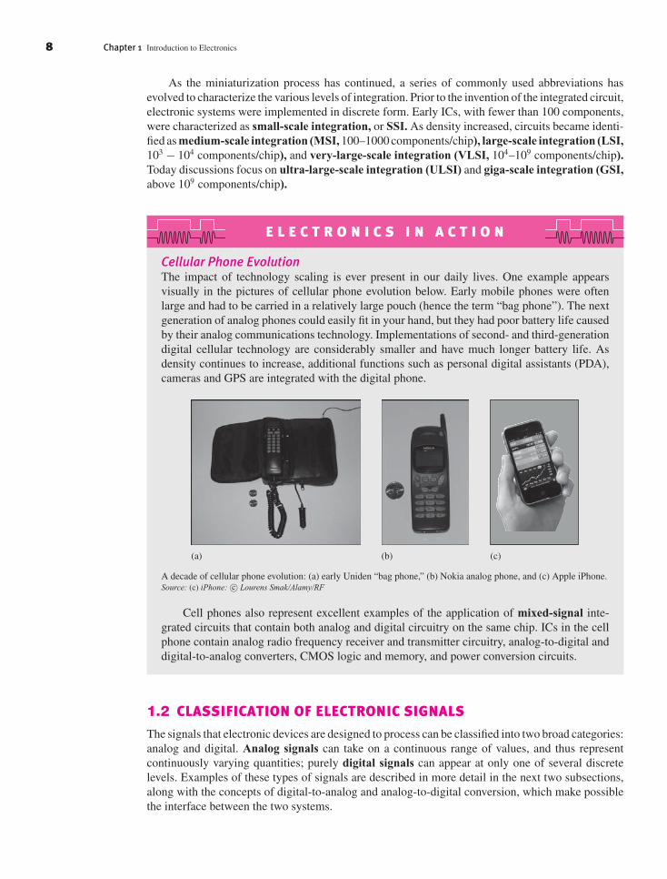
Jaeger-1820037 book January 15, 2010 21:25
8 Chapter 1 Introduction to Electronics
As the miniaturization process has continued, a series of commonly used abbreviations hasevolved to characterize the various levels of integration. Prior to the invention of the integrated circuit,electronic systems were implemented in discrete form. Early ICs, with fewer than 100 components,were characterized as small-scale integration, or SSI. As density increased, circuits became identi-fied as medium-scale integration (MSI, 100–1000 components/chip), large-scale integration (LSI,103 − 104 components/chip), and very-large-scale integration (VLSI, 104–109 components/chip).Today discussions focus on ultra-large-scale integration (ULSI) and giga-scale integration (GSI,above 109 components/chip).
E L E C T R O N I C S I N A C T I O N
Cellular Phone EvolutionThe impact of technology scaling is ever present in our daily lives. One example appearsvisually in the pictures of cellular phone evolution below. Early mobile phones were oftenlarge and had to be carried in a relatively large pouch (hence the term “bag phone”). The nextgeneration of analog phones could easily fit in your hand, but they had poor battery life causedby their analog communications technology. Implementations of second- and third-generationdigital cellular technology are considerably smaller and have much longer battery life. Asdensity continues to increase, additional functions such as personal digital assistants (PDA),cameras and GPS are integrated with the digital phone.
(a) (b) (c)
A decade of cellular phone evolution: (a) early Uniden “bag phone,” (b) Nokia analog phone, and (c) Apple iPhone.Source: (c) iPhone: c© Lourens Smak/Alamy/RF
Cell phones also represent excellent examples of the application of mixed-signal inte-grated circuits that contain both analog and digital circuitry on the same chip. ICs in the cellphone contain analog radio frequency receiver and transmitter circuitry, analog-to-digital anddigital-to-analog converters, CMOS logic and memory, and power conversion circuits.
1.2 CLASSIFICATION OF ELECTRONIC SIGNALS
The signals that electronic devices are designed to process can be classified into two broad categories:analog and digital. Analog signals can take on a continuous range of values, and thus representcontinuously varying quantities; purely digital signals can appear at only one of several discretelevels. Examples of these types of signals are described in more detail in the next two subsections,along with the concepts of digital-to-analog and analog-to-digital conversion, which make possiblethe interface between the two systems.

Jaeger-1820037 book January 15, 2010 21:25
1.2 Classification of Electronic Signals 9
Amplitude
Highlevel
Lowlevel
1
0t
Figure 1.6 A time-varying binary digital signal.
1.2.1 DIGITAL SIGNALSWhen we speak of digital electronics, we are most often referring to electronic processing of binarydigital signals, or signals that can take on only one of two discrete amplitude levels as illustrated inFig. 1.6. The status of binary systems can be represented by two symbols: a logical 1 is assigned torepresent one level, and a logical 0 is assigned to the second level.2 The two logic states generallycorrespond to two separate voltages—VH and VL—representing the high and low amplitude levels,and a number of voltage ranges are in common use. Although VH = 5 V and VL = 0 V representedthe primary standard for many years, these have given way to lower voltage levels because of powerconsumption and semiconductor device limitations. Systems employing VH = 3.3, 2.5, and 1.5 V,with VL = 0 V, are now used in many types of electronics.
However, binary voltage levels can also be negative or even bipolar. One high-performancelogic family called ECL uses VH = −0.8 V and VL = −2.0 V, and the early standard RS-422 andRS-232 communication links between a small computer and its peripherals used VH = +12 V andVL = −12 V. In addition, the time-varying binary signal in Fig. 1.6 could equally well represent theamplitude of a current or that of an optical signal being transmitted down a fiber in an optical digitalcommunication system. The more recent USB and Firewire standards returned to the use of a singlepositive supply voltage.
Part II of this text discusses the design of a number of families of digital circuits using varioussemiconductor technologies. These include CMOS,3 NMOS, and PMOS logic, which use field-effecttransistors, and the TTL and ECL families, which are based on bipolar transistors.
1.2.2 ANALOG SIGNALSAlthough quantities such as electronic charge and electron spin are truly discrete, much of thephysical world is really analog in nature. Our senses of vision, hearing, smell, taste, and touchare all analog processes. Analog signals directly represent variables such as temperature, humidity,pressure, light intensity, or sound—all of which may take on any value, typically within some finiterange. In reality, classification of digital and analog signals is largely one of perception. If we lookat a digital signal similar to the one in Fig. 1.6 with an oscilloscope, we find that it actually makes acontinuous transition between the high and low levels. The signal cannot make truly abrupt transitionsbetween two levels. Designers of high-speed digital systems soon realize that they are really dealingwith analog signals. The time-varying voltage or current plotted in Fig. 1.7 could be the electricalrepresentation of temperature, flow rate, or pressure versus time, or the continuous audio output froma microphone. Some analog transducers produce output voltages in the range of 0 to 5 or 0 to 10 V,whereas others are designed to produce an output current that ranges between 4 and 20 mA. At theother extreme, signals brought in by a radio antenna can be as small as a fraction of a microvolt.
To process the information contained in these analog signals, electronic circuits are used to se-lectively modify the amplitude, phase, and frequency content of the signals. In addition, significant
2 This assignment facilitates the use of Boolean algebra, reviewed in Chapter 6.3 For now, let us accept these initials as proper names without further definition. The details of each of these circuits are developed in
Part II.
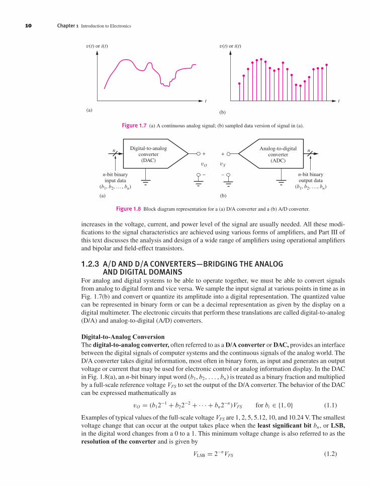
Jaeger-1820037 book January 15, 2010 21:25
10 Chapter 1 Introduction to Electronics
t
v(t) or i(t)
(a)
t
v(t) or i(t)
(b)
Figure 1.7 (a) A continuous analog signal; (b) sampled data version of signal in (a).
Digital-to-analogconverter
(DAC)+
–
vO
n-bit binaryinput data
(b1, b2, …, bn)
n
(a) (b)
Analog-to-digitalconverter(ADC)vX
n-bit binaryoutput data
(b1, b2, …, bn)
n+
–
Figure 1.8 Block diagram representation for a (a) D/A converter and a (b) A/D converter.
increases in the voltage, current, and power level of the signal are usually needed. All these modi-fications to the signal characteristics are achieved using various forms of amplifiers, and Part III ofthis text discusses the analysis and design of a wide range of amplifiers using operational amplifiersand bipolar and field-effect transistors.
1.2.3 A/D AND D/A CONVERTERS—BRIDGING THE ANALOGAND DIGITAL DOMAINS
For analog and digital systems to be able to operate together, we must be able to convert signalsfrom analog to digital form and vice versa. We sample the input signal at various points in time as inFig. 1.7(b) and convert or quantize its amplitude into a digital representation. The quantized valuecan be represented in binary form or can be a decimal representation as given by the display on adigital multimeter. The electronic circuits that perform these translations are called digital-to-analog(D/A) and analog-to-digital (A/D) converters.
Digital-to-Analog ConversionThe digital-to-analog converter, often referred to as a D/A converter or DAC, provides an interfacebetween the digital signals of computer systems and the continuous signals of the analog world. TheD/A converter takes digital information, most often in binary form, as input and generates an outputvoltage or current that may be used for electronic control or analog information display. In the DACin Fig. 1.8(a), an n-bit binary input word (b1, b2, . . . , bn) is treated as a binary fraction and multipliedby a full-scale reference voltage VFS to set the output of the D/A converter. The behavior of the DACcan be expressed mathematically as
vO = (b12−1 + b22−2 + · · · + bn2−n)VFS for bi ∈ {1, 0} (1.1)
Examples of typical values of the full-scale voltage VFS are 1, 2, 5, 5.12, 10, and 10.24 V. The smallestvoltage change that can occur at the output takes place when the least significant bit bn , or LSB,in the digital word changes from a 0 to a 1. This minimum voltage change is also referred to as theresolution of the converter and is given by
VLSB = 2−n VFS (1.2)

Jaeger-1820037 book January 15, 2010 21:25
1.2 Classification of Electronic Signals 11
111
110
101
100
011
010
001
0000 VFSVFS
2
1 LSB
43VFS
43VFS
Bin
ary
outp
ut c
ode
(b1b
2b 3
)
Input voltage
(a)
1.5
0.5
–0.5
–1.50 VFSVFS
4VFS
2
Qua
ntiz
atio
n er
ror
(LSB
)
Input voltage
1 LSB
(b)
VFS
4
Figure 1.9 (a) Input–output relationship and (b) quantization error for 3-bit ADC.
At the other extreme, b1 is referred to as the most significant bit, or MSB, and has a weight ofone-half VFS.
Exercise: A 10-bit D/A converter has VF S = 5.12 V. What is the output voltage for a binaryinput code of (1100010001)? What is VLSB? What is the size of the MSB?
Answers: 3.925 V; 5 mV; 2.56 V
Analog-to-Digital ConversionThe analog-to-digital converter (A/D converter or ADC) is used to transform analog informationin electrical form into digital data. The ADC in Fig. 1.8(b) takes an unknown continuous analoginput signal, usually a voltage vX , and converts it into an n-bit binary number that can be easilymanipulated by a computer. The n-bit number is a binary fraction representing the ratio between theunknown input voltage vX and the converter’s full-scale voltage VFS.
For example, the input–output relationship for an ideal 3-bit A/D converter is shown in Fig. 1.9(a).As the input increases from zero to full scale, the output digital code word stair-steps from 000 to111.4 The output code is constant for an input voltage range equal to 1 LSB of the ADC. Thus, asthe input voltage increases, the output code first underestimates and then overestimates the inputvoltage. This error, called quantization error, is plotted against input voltage in Fig. 1.9(b).
For a given output code, we know only that the value of the input voltage lies somewhere within a1-LSB quantization interval. For example, if the output code of the 3-bit ADC is 100, correspondingto a voltage VFS/2, then the input voltage can be anywhere between 7
16 VFS and 916 VFS, a range of
VFS/8 V or 1 LSB. From a mathematical point of view, the ADC circuitry in Fig. 1.8(b) picks thevalues of the bits in the binary word to minimize the magnitude of the quantization error vε betweenthe unknown input voltage vX and the nearest quantized voltage level:
vε = |vX − (b12−1 + b22−2 + · · · + bn2−n)VFS| (1.3)
4 The binary point is understood to be to the immediate left of the digits of the code word. As the code word stair-steps from 000 to 111,the binary fraction steps from 0.000 to 0.111.

Jaeger-1820037 book January 15, 2010 21:25
12 Chapter 1 Introduction to Electronics
Exercise: An 8-bit A/D converter has VF S = 5 V. What is the digital output code word for aninput of 1.2 V? What is the voltage range corresponding to 1 LSB of the converter?
Answers: 00111101; 19.5 mV
1.3 NOTATIONAL CONVENTIONS
In many circuits we will be dealing with both dc and time-varying values of voltages and currents.The following standard notation will be used to keep track of the various components of an electricalsignal. Total quantities will be represented by lowercase letters with capital subscripts, such as vT
and iT in Eq. (1.4). The dc components are represented by capital letters with capital subscripts as,for example, VDC and IDC in Eq. (1.4); changes or variations from the dc value are represented bysignal components vsig and isig.
vT = VDC + vsig or iT = IDC + isig (1.4)
As examples, the total base-emitter voltage vBE of a transistor and the total drain current iD of afield-effect transistor are written as
vBE = VBE + vbe and iD = ID + id (1.5)
Unless otherwise indicated, the equations describing a given network will be written assuminga consistent set of units: volts, amperes, and ohms. For example, the equation 5 V = (10,000 �)I1 +0.6 V will be written as 5 = 10,000I1 + 0.6.
The fourth upper/lowercase combination, such as Vbe or Id , is reserved for the amplitude of asinusoidal signal’s phasor representation as defined in Section 1.7.
Exercise: Suppose the voltage at a circuit node is described by
vA = (5 sin 2000π t + 4 + 3 cos 1000πt) V
What are the expressions for VA and va?
Answers: VA = 4 V; va = (5 sin 2000π t + 3 cos 1000π t) V
Resistance and Conductance RepresentationsIn the circuits throughout this text, resistors will be indicated symbolically as Rx or rx , and the valueswill be expressed in �, k�, M�, and so on. During analysis, however, it may be more convenient towork in terms of conductance with the following convention:
Gx = 1
Rxand gπ = 1
rπ
(1.6)
For example, conductance Gx always represents the reciprocal of the value of Rx , and gπ representsthe reciprocal of rπ . The values next to a resistor symbol will always be expressed in terms ofresistance (�, k�, M�).
Dependent SourcesIn electronics, dependent (or controlled) sources are used extensively. Four types of dependentsources are summarized in Fig. 1.10, in which the standard diamond shape is used for controlledsources. The voltage-controlled current source (VCCS), current-controlled current source(CCCS), and voltage-controlled voltage source (VCVS) are used routinely in this text to model

Jaeger-1820037 book January 15, 2010 21:25
1.4 Problem-Solving Approach 13
gmv1
(a) VCCS
v1
–
+
Av1
(c) VCVS
v1
–
+
�i1
(b) CCCS
i1 Ki1i1
(d) CCVS
Figure 1.10 Controlled sources. (a) Voltage-controlled current source (VCCS). (b) Current-controlled current source(CCCS). (c) Voltage-controlled voltage source (VCVS). (d) Current-controlled voltage source (CCVS).
transistors and amplifiers or to simplify more complex circuits. Only the current-controlled voltagesource (CCVS) sees limited use.
1.4 PROBLEM-SOLVING APPROACH
Solving problems is a centerpiece of an engineer’s activity. As engineers, we use our creativity tofind new solutions to problems that are presented to us. A well-defined approach can aid signi-ficantly in solving problems. The examples in this text highlight an approach that can be used inall facets of your career, as a student and as an engineer in industry. The method is outlined in thefollowing nine steps:
1. State the problem as clearly as possible.2. List the known information and given data.3. Define the unknowns that must be found to solve the problem.4. List your assumptions. You may discover additional assumptions as the analysis progresses.5. Develop an approach from a group of possible alternatives.6. Perform an analysis to find a solution to the problem. As part of the analysis, be sure to draw
the circuit and label the variables.7. Check the results. Has the problem been solved? Is the math correct? Have all the unknowns
been found? Have the assumptions been satisfied? Do the results satisfy simple consistencychecks?
8. Evaluate the solution. Is the solution realistic? Can it be built? If not, repeat steps 4–7 until asatisfactory solution is obtained.
9. Computer-aided analysis. SPICE and other computer tools are highly useful to check the resultsand to see if the solution satisfies the problem requirements. Compare the computer results toyour hand results.
To begin solving a problem, we must try to understand its details. The first four steps, whichattempt to clearly define the problem, can be the most important part of the solution process. Timespent understanding, clarifying, and defining the problem can save much time and frustration.
The first step is to write down a statement of the problem. The original problem description maybe quite vague; we must try to understand the problem as well as, or even better than, the individualwho posed the problem. As part of this focus on understanding the problem, we list the informationthat is known and unknown. Problem-solving errors can often be traced to imprecise definition ofthe unknown quantities. For example, it is very important for analysis to draw the circuit properlyand to clearly label voltages and currents on our circuit diagrams.
Often there are more unknowns than constraints, and we need engineering judgment to reacha solution. Part of our task in studying electronics is to build up the background for selectingbetween various alternatives. Along the way, we often need to make approximations and assumptionsthat simplify the problem or form the basis of the chosen approach. It is important to state theseassumptions, so that we can be sure to check their validity at the end. Throughout this text youwill encounter opportunities to make assumptions. Most often, you should make assumptions thatsimplify your computational effort yet still achieve useful results.

Jaeger-1820037 book January 15, 2010 21:25
14 Chapter 1 Introduction to Electronics
The exposition of the known information, unknowns, and assumptions helps us not only tobetter understand the problem but also to think about various alternative solutions. We must choosethe approach that appears to have the best chance of solving the problem. There may be morethan one satisfactory approach. Each person will view the problem somewhat differently, and theapproach that is clearest to one individual may not be the best for another. Pick the one that seemsbest to you. As part of defining the approach, be sure to think about what computational tools areavailable to assist in the solution, including MATLAB® , Mathcad® , spreadsheets, SPICE, and yourcalculator.
Once the problem and approach are defined as clearly as possible, then we can perform anyanalysis required and solve the problem. After the analysis is completed we need to check theresults. A number of questions should be resolved. First, have all the unknowns been found? Do theresults make sense? Are they consistent with each other? Are the results consistent with assumptionsused in developing the approach to the problem?
Then we need to evaluate the solution. Are the results viable? For example, are the voltage, cur-rent, and power levels reasonable? Can the circuit be realized with reasonable yield with real compo-nents? Will the circuit continue to function within specifications in the face of significant componentvariations? Is the cost of the circuit within specifications? If the solution is not satisfactory, weneed to modify our approach and assumptions and attempt a new solution. An iterative solution isoften required to meet the specifications in realistic design situations. SPICE and other computertools are highly useful for checking results and ensuring that the solution satisfies the problemrequirements.
The solutions to the examples in this text have been structured following the problem-solvingapproach introduced here. Although some examples may appear trivial, the power of the structuredapproach increases as the problem becomes more complex.
WHAT ARE REASONABLE NUMBERS?
Part of our results check should be to decide if the answer is “reasonable” and makes sense. Overtime we must build up an understanding of what numbers are reasonable. Most solid-state devicesthat we will encounter are designed to operate from voltages ranging from a battery voltage of 1 Von the low end to no more than 40–50 V5 at the high end. Typical power supply voltages will bein the 10- to 20-V range, and typical resistance values encountered will range from tens of � up tomany G�.
Based on our knowledge of dc circuits, we should expect that the voltages in our circuitsnot exceed the power supply voltages. For example, if a circuit is operating from +8- and −5-Vsupplies, all of our calculated dc voltages must be between −5 and +8 V. In addition, the peak-to-peakamplitude of an ac signal should not exceed 13 V, the difference of the two supply voltages. Witha 10-V supply, the maximum current that can go through a 100-� resistor is 100 mA; the currentthrough a 10-M� resistor can be no more than 1 �A. Thus we should remember the following “rules”to check our results:
1. With few exceptions, the dc voltages in our circuits cannot exceed the power supply voltages.The peak-to-peak amplitude of an ac signal should not exceed the difference of the power supplyvoltages.
2. The currents in our circuits will range from microamperes to no more than a hundred milliamperesor so.
5 The primary exception is in the area of power electronics, where one encounters much larger voltages and currents than the onesdiscussed here.

Jaeger-1820037 book January 15, 2010 21:25
1.5 Important Concepts from Circuit Theory 15
1.5 IMPORTANT CONCEPTS FROM CIRCUIT THEORY
Analysis and design of electronic circuits make continuous use of a number of important tech-niques from basic network theory. Circuits are most often analyzed using a combination ofKirchhoff’s voltage law, abbreviated KVL, and Kirchhoff’s current law, abbreviated KCL.Occasionally, the solution relies on systematic application of nodal or mesh analysis. Theveninand Norton circuit transformations are often used to help simplify circuits, and the notions ofvoltage and current division also represent basic tools of analysis. Models of active devices invari-ably involve dependent sources, as mentioned in the last section, and we need to be familiar withdependent sources in all forms. Amplifier analysis also uses two-port network theory. A review oftwo-port networks is deferred until the introductory discussion of amplifiers in Chapter 10. If thereader feels uncomfortable with any of the concepts just mentioned, this is a good time for review.To help, a brief review of these important circuit techniques follows.
1.5.1 VOLTAGE AND CURRENT DIVISIONVoltage and current division are highly useful circuit analysis techniques that can be derived directlyfrom basic circuit theory. They are both used routinely throughout this text, and it is very importantto be sure to understand the conditions for which each technique is valid! Examples of both methodsare provided next.
Voltage division is demonstrated by the circuit in Fig. 1.11(a) in which the voltages v1 and v2
can be expressed as
v1 = ii R1 and v2 = ii R2 (1.7)
Applying KVL to the single loop,
vi = v1 + v2 = ii (R1 + R2) and ii = vi
R1 + R2(1.8)
Combining Eqs. (1.7) and (1.8) yields the basic voltage division formula:
v1 = viR1
R1 + R2and v2 = vi
R2
R1 + R2(1.9)
For the resistor values in Fig. 1.11(a),
v1 = 10 V8 k�
8 k� + 2 k�= 8.00 V and v2 = 10 V
2 k�
8 k� + 2 k�= 2.00 V (1.10)
R1 8 k�
v2
v1
vi
+
–ii
R2
+ –
2 k�10 V3 k�
ii
5 mA
i2R1 R2
2 k�
i1
vi
+
–
(a) (b)
Figure 1.11 (a) A resistive voltage divider, (b) Current division in a simple network.

Jaeger-1820037 book January 15, 2010 21:25
16 Chapter 1 Introduction to Electronics
Note that the voltage divider relationships in Eq. (1.9) can be applied only when the current throughthe two resistor branches is the same. Also, note that the formulas are correct if the resistancesare replaced by complex impedances and the voltages are represented as phasors.
V1 = VSZ1
Z1 + Z2and V2 = VS
Z2
Z1 + Z2
VOLTAGE DIVIDER RESTRICTIONSDESIGNNOTE
Current division is also very useful. Let us find the currents i1 and i2 in the circuit in Fig. 1.11(b).Using KCL at the single node,
ii = i1 + i2 where i1 = vi
R1and i2 = vi
R2(1.11)
and solving for vS yields
vi = ii1
1
R1+ 1
R2
= iiR1 R2
R1 + R2= ii (R1‖R2) (1.12)
in which the notation R1‖R2 represents the parallel combination of resistors R1 and R2. CombiningEqs. (1.11) and (1.12) yields the current division formulas:
i1 = iiR2
R1 + R2and i2 = ii
R1
R1 + R2(1.13)
For the values in Fig. 1.11(b),
i1 = 5 mA3 k�
2 k� + 3 k�= 3.00 mA i2 = 5 mA
2 k�
2 k� + 3 k�= 2.00 mA
It is important to note that the same voltage must appear across both resistors in order for thecurrent division expressions in Eq. (1.13) to be valid. Here again, the formulas are correct if theresistances are replaced by complex impedances and the currents are represented as phasors.
I1 = ISZ2
Z1 + Z2and I2 = IS
Z1
Z1 + Z2
CURRENT DIVIDER RESTRICTIONSDESIGNNOTE
1.5.2 THEVENIN AND NORTON CIRCUIT REPRESENTATIONSLet us now review the method for finding Thevenin and Norton equivalent circuits, including adependent source; the circuit in Fig. 1.12(a) serves as our illustration. Because the linear network in thedashed box has only two terminals, it can be represented by either the Thevenin or Norton equivalentcircuits in Figs. 1.12(b) and 1.12(c). The work of Thevenin and Norton permits us to reduce complexcircuits to a single source and equivalent resistance. We illustrate these two important techniqueswith the next four examples.

Jaeger-1820037 book January 15, 2010 21:25
1.5 Important Concepts from Circuit Theory 17
20 k�
R1
RS 1 k�vi
� = 50
vo
+
_
�i1
i1
in
R th
R th
(b)(a)
vth
(c)
Figure 1.12 (a) Two-terminal circuit and its (b) Thevenin and (c) Norton equivalents.
EXAMPLE 1.1 THEVENIN AND NORTON EQUIVALENT CIRCUITS
Let’s practice finding the Thevenin and Norton equivalent circuits for the network in Fig. 1.12(a).
PROBLEM Find the Thevenin and Norton equivalent representations for the circuit in Fig. 1.12(a).
SOLUTION Known Information and Given Data: Circuit topology and values appear in Fig. 1.12(a).
Unknowns: Thevenin equivalent voltage vth, Thevenin equivalent resistance Rth, and Nortonequivalent current in .
Approach: Voltage source vth is defined as the open-circuit voltage at the terminals of the circuit.Rth is the equivalent at the terminals of the circuit terminals with all independent sources set tozero. Source in represents the short-circuit current available at the output terminals and is equal tovth/Rth.
Assumptions: None
Analysis: We will first find the value of vth, then Rth and finally in . Open-circuit voltage vth canbe found by applying KCL at the output terminals.
βi1 = vo − vi
R1+ vo
RS= G1(vo − vi ) + GSvo (1.14)
by applying the notational convention for conductance from Sec. 1.3 (GS = 1/RS).Current i1 is given by
i1 = G1(vi − vo) (1.15)
Substituting Eq. (1.15) into Eq. (1.14) and combining terms yields
G1(β + 1)vi = [G1(β + 1) + GS]vo (1.16)
The Thevenin equivalent output voltage is then found to be
vo = G1(β + 1)
[G1(β + 1) + GS]vi = (β + 1)RS
[(β + 1)RS + R1]vi (1.17)
where the second relationship was found by multiplying numerator and denominator by (R1 RS).For the values in this problem,
vo = (50 + 1)1 k�
[(50 + 1) 1 k� + 20 k�]vi = 0.718vi and vth = 0.718vi (1.18)
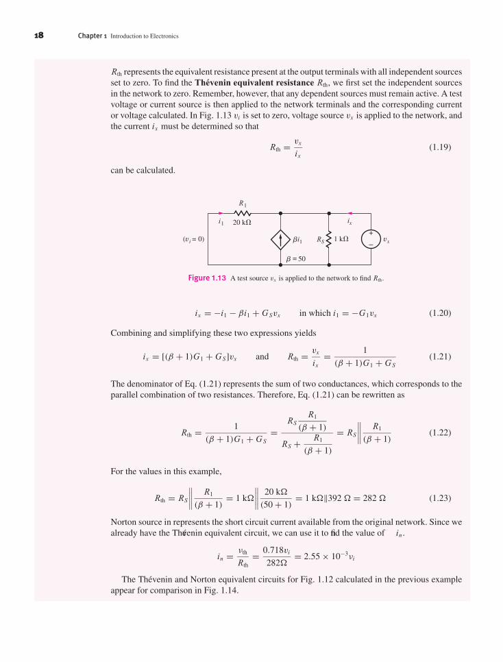
Jaeger-1820037 book January 15, 2010 21:25
18 Chapter 1 Introduction to Electronics
Rth represents the equivalent resistance present at the output terminals with all independent sourcesset to zero. To find the Thevenin equivalent resistance Rth, we first set the independent sourcesin the network to zero. Remember, however, that any dependent sources must remain active. A testvoltage or current source is then applied to the network terminals and the corresponding currentor voltage calculated. In Fig. 1.13 vi is set to zero, voltage source vx is applied to the network, andthe current ix must be determined so that
Rth = vx
ix(1.19)
can be calculated.
RS�i1 1 k�
20 k�i1 ix
R1
vx(vi = 0)
� = 50
Figure 1.13 A test source vx is applied to the network to find Rth.
ix = −i1 − βi1 + GSvx in which i1 = −G1vx (1.20)
Combining and simplifying these two expressions yields
ix = [(β + 1)G1 + GS]vx and Rth = vx
ix= 1
(β + 1)G1 + GS(1.21)
The denominator of Eq. (1.21) represents the sum of two conductances, which corresponds to theparallel combination of two resistances. Therefore, Eq. (1.21) can be rewritten as
Rth = 1
(β + 1)G1 + GS=
RSR1
(β + 1)
RS + R1
(β + 1)
= RS
∥∥∥∥ R1
(β + 1)(1.22)
For the values in this example,
Rth = RS
∥∥∥∥ R1
(β + 1)= 1 k�
∥∥∥∥ 20 k�
(50 + 1)= 1 k�‖392 � = 282 � (1.23)
Norton source in represents the short circuit current available from the original network. Since wealready have the Thévenin equivalent circuit, we can use it to find the value of in .
in = νth
Rth= 0.718vi
282�= 2.55 × 10⁻³νi
The Thevenin and Norton equivalent circuits for Fig. 1.12 calculated in the previous exampleappear for comparison in Fig. 1.14.

Jaeger-1820037 book January 15, 2010 21:25
1.5 Important Concepts from Circuit Theory 19
in
R th = 282 �
R th = 282 �
(a)
vth
vth = 0.718vs
(b)
in = (2.55 �10–3)vs
Figure 1.14 Completed (a) Thevenin and (b) Norton equivalent circuits for the two-terminal network in Fig. 1.12(a).
Check of Results: We have found the three unknowns required. A recheck of the calculationsindicates they are done correctly. The value of vth is the same order of magnitude as vi , so its valueshould not be unusually large or small. The value of Rth is less than 1 k�, which seems reasonable,since we should not expect the resistance to exceed the value of RS that appears in parallel withthe output terminals. We can double-check everything by directly calculating in from the originalcircuit. If we short the output terminals in Fig. 1.12, we find the short-circuit current (See Ex. 1.2)to be in = (β + 1) vi/R1 = 2.55 × 10⁻³vi and in agreement with the other method.
EXAMPLE 1.2 NORTON EQUIVALENT CIRCUIT
Practice finding the Norton equivalent circuit for a network containing a dependent source.
PROBLEM Find the Norton equivalent (Fig. 1.12(c)) for the circuit in Fig. 1.12(a).
SOLUTION Known Information and Given Data: Circuit topology and circuit values appear in Fig. 1.12(a).The value of Rth was calculated in the previous example.
Unknowns: Norton equivalent current in .
Approach: The Norton equivalent current is found by determining the current coming out of thenetwork when a short circuit is applied to the terminals.
Assumptions: None.
Analysis: For the circuit in Fig. 1.15, the output current will be
in = i1 + βi1 and i1 = G1vi (1.24)
The short circuit across the output forces the current through RS to be 0. Combining the twoexpressions in Eq. (1.24) yields
in = (β + 1)G1vi = (β + 1)
R1vi (1.25)
or
in = (50 + 1)
20 k�vi = vi
392 �= (2.55 mS)vi (1.26)
The resistance in the Norton equivalent circuit also equals Rth found in Eq. (1.23).

Jaeger-1820037 book January 20, 2010 14:36
20 Chapter 1 Introduction to Electronics
RS
0
1 k�
20 k�
in
i1
R1
vi
� = 50
�i1
Figure 1.15 Circuit for determining short-circuit output current.
Check of Results: We have found the Norton equivalent current. Note that vth = in Rth and thisresult can be used to check the calculations: in Rth = (2.55 mS)vs(282 �) = 0.719 vs , whichagrees within round-off error with the previous example.
E L E C T R O N I C S I N A C T I O N
Player CharacteristicsThe headphone amplifier in a personal music player represents an everyday example of a basicaudio amplifier. The traditional audio band spans the frequencies from 20 Hz to 20 kHz, a rangethat extends beyond the hearing capability of most individuals at both the upper and lower ends.
iPod: c© The McGraw-HillCompanies, Inc./Jill Braaten,
photographer
vth
Rth
32 �
2 V
Thevenin equivalentcircuit for output stage
The characteristics of the Apple iPod in the accompanying figure are representative of a highquality audio output stage in an MP3 player or a computer sound card. The output can berepresented by a Thevenin equivalent circuit with vth = 2 V and Rth = 32 ohms, and theoutput stage is designed to deliver a power of approximately 15 mW into each channel of aheadphone with a matched impedance of 32 ohms. The output power is approximately constantover the 20 Hz–20 kHz frequency range. At the lower and upper cutoff frequencies, fL andfH , the output power will be reduced by 3 dB, a factor of 2.

Jaeger-1820037 book January 15, 2010 21:25
1.6 Frequency Spectrum of Electronic Signals 21
fL fH
20 Hz 20 kHzFrequency
Out
put p
ower Pmid
Power versus frequency for an audio amplifier
The distortion characteristics of the amplifier are also important, and this is an area thatoften distinguishes one sound card or MP3 player from another. A good audio system willhave a total harmonic distortion (THD) specification of less than 0.1 percent at full power.
1.6 FREQUENCY SPECTRUM OF ELECTRONIC SIGNALS
Fourier analysis and the Fourier series represent extremely powerful tools in electrical engineering.Results from Fourier theory show that complicated signals are actually composed of a continuumof sinusoidal components, each having a distinct amplitude, frequency, and phase. The frequencyspectrum of a signal presents the amplitude and phase of the components of the signal versusfrequency.
Nonrepetitive signals have continuous spectra with signals that may occupy a broad range offrequencies. For example, the amplitude spectrum of a television signal measured during a smalltime interval is depicted in Fig. 1.16. The TV video signal is designed to occupy the frequency rangefrom 0 to 4.5 MHz.6 Other types of signals occupy different regions of the frequency spectrum.Table 1.3 identifies the frequency ranges associated with various categories of common signals.
In contrast to the continuous spectrum in Fig. 1.16, Fourier series analysis shows that anyperiodic signal, such as the square wave of Fig. 1.17, contains spectral components only at discretefrequencies7 that are related directly to the period of the signal. For example, the square wave ofFig. 1.17 having an amplitude VO and period T can be represented by the Fourier series
v(t) = VDC + 2VO
π
(sin ωot + 1
3sin 3ωot + 1
5sin 5ωot + · · ·
)(1.27)
in which ωo = 2π/T (rad/s) is the fundamental radian frequency of the square wave. We refer tofo = 1/T (Hz) as the fundamental frequency of the signal, and the frequency components at 2 fo,3 fo, 4 fo, . . . are called the second, third, fourth, and so on harmonic frequencies.
6 This signal is combined with a much higher carrier frequency prior to transmission.7 There are an infinite number of components, however.
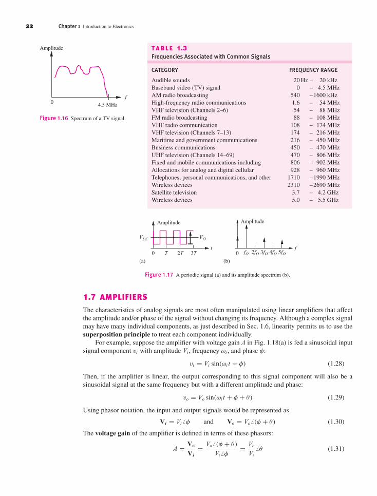
Jaeger-1820037 book January 15, 2010 21:25
22 Chapter 1 Introduction to Electronics
Amplitude
0 4.5 MHzf
Figure 1.16 Spectrum of a TV signal.
T A B L E 1.3Frequencies Associated with Common Signals
CATEGORY FREQUENCY RANGE
Audible sounds 20 Hz – 20 kHzBaseband video (TV) signal 0 – 4.5 MHzAM radio broadcasting 540 –1600 kHzHigh-frequency radio communications 1.6 – 54 MHzVHF television (Channels 2–6) 54 – 88 MHzFM radio broadcasting 88 – 108 MHzVHF radio communication 108 – 174 MHzVHF television (Channels 7–13) 174 – 216 MHzMaritime and government communications 216 – 450 MHzBusiness communications 450 – 470 MHzUHF television (Channels 14–69) 470 – 806 MHzFixed and mobile communications including 806 – 902 MHzAllocations for analog and digital cellular 928 – 960 MHzTelephones, personal communications, and other 1710 –1990 MHzWireless devices 2310 –2690 MHzSatellite television 3.7 – 4.2 GHzWireless devices 5.0 – 5.5 GHz
Amplitude
(a) (b)
0 T 2T 3T
VDC VO
t
Amplitude
0 fO 2fO 3fO 4fO 5fOf
Figure 1.17 A periodic signal (a) and its amplitude spectrum (b).
1.7 AMPLIFIERS
The characteristics of analog signals are most often manipulated using linear amplifiers that affectthe amplitude and/or phase of the signal without changing its frequency. Although a complex signalmay have many individual components, as just described in Sec. 1.6, linearity permits us to use thesuperposition principle to treat each component individually.
For example, suppose the amplifier with voltage gain A in Fig. 1.18(a) is fed a sinusoidal inputsignal component vi with amplitude Vi , frequency ωi , and phase φ:
vi = Vi sin(ωi t + φ) (1.28)
Then, if the amplifier is linear, the output corresponding to this signal component will also be asinusoidal signal at the same frequency but with a different amplitude and phase:
vo = Vo sin(ωi t + φ + θ) (1.29)
Using phasor notation, the input and output signals would be represented as
Vi = Vi � φ and Vo = Vo � (φ + θ) (1.30)
The voltage gain of the amplifier is defined in terms of these phasors:
A = Vo
Vi= Vo � (φ + θ)
Vi � φ= Vo
Vi
� θ (1.31)

Jaeger-1820037 book January 15, 2010 21:25
1.7 Amplifiers 23
vi vo = Avi
A+
–
+
–
(a)
vivo = Avi
A+
–
+
–+
–
(b)
Figure 1.18 (a) Symbol for amplifierwith single input and voltage gain A;(b) differential amplifier having twoinputs and gain A.
0
–2
–4
–6
2
4
6
Time (sec)
v o (
volts
)
0 0.0005 0.001 0.0015 0.002 0.0025
Input voltageOutput voltage
Inverting amplifier
Figure 1.19 Input and output voltage waveforms for an amplifier with gainAv = −5 and vi = 1 sin 2000π t V.
This amplifier has a voltage gain with magnitude equal to Vo/Vi and a phase shift of θ . In general,both the magnitude and phase of the voltage gain will be a function of frequency. Note that amplifiersalso often provide current gain and power gain as well as voltage gain, but these concepts will notbe explored further until Chapter 10.
The curves in Fig. 1.19 represent the input and output voltage waveforms for an invertingamplifier with Av = −5 and vi = 1 sin 2000π t V. Both the factor of five increase in signal amplitudeand the 180◦ phase shift (multiplication by −1) are apparent in the graph.
At this point, a note regarding the phase angle is needed. In Eqs. (1.28) and (1.29), ωt , φ, andθ must have the same units. With ωt normally expressed in radians, φ should also be in radians.However, in electrical engineering texts, φ is often expressed in degrees. We must be aware of thismixed system of units and remember to convert degrees to radians before making any numericcalculations.
Exercise: The input and output voltages of an amplifier are expressed as
vi = 0.001 sin(2000πt) V and vo = −5 cos(2000πt + 25◦) V
in which vi and vo are specified in volts when t is seconds. What are Vi, VO, and the voltagegain of the amplifier?
Answers: 0.001� 0◦; 5� −65◦; 5000� −65◦
1.7.1 IDEAL OPERATIONAL AMPLIFIERSThe operational amplifier, “op amp” for short, is a fundamental building block in electronic designand is discussed in most introductory circuit courses. A brief review of the ideal op amp is providedhere; an in-depth study of the properties of ideal and nonideal op amps and the circuits used to buildthe op amp itself are the subjects of Chapters 11, 12, 15, and 16. Although it is impossible to realizethe ideal operational amplifier, its use allows us to quickly understand the basic behavior to beexpected from a given circuit and serves as a model to help in circuit design.