Chronic Kidney Disease Mortality in Costa Rica ...
121
LUMA-GIS Thesis nr 39 Negin A Sanati 2015 Department of Physical Geography and Ecosystem Science Centre for Geographical Information Systems Lund University Sölvegatan 12 S-223 62 Lund Sweden Chronic Kidney Disease Mortality in Costa Rica; Geographical Distribution, Spatial Analysis and Non-traditional Risk Factors
Transcript of Chronic Kidney Disease Mortality in Costa Rica ...

LUMA-GIS Thesis nr 39
Negin A Sanati
2015 Department of Physical Geography and Ecosystem Science Centre for Geographical Information Systems Lund University Sölvegatan 12 S-223 62 Lund Sweden
Chronic Kidney Disease Mortality in Costa
Rica; Geographical Distribution, Spatial
Analysis and Non-traditional Risk Factors

i
Negin A Sanati (2015). Chronic Kidney Disease Mortality in Costa Rica; Geographical
Distribution, Spatial Analysis and Non-traditional Risk Factors
Master degree thesis, 30 credits in Master in Geographical Information Sciences
Department of Physical Geography and Ecosystems Science, Lund University
Level: Master of Science (MSc)
Course duration: September 2014 until March 2015
Disclaimer
This document describes work undertaken as part of a program of study at the University of
Lund. All views and opinions expressed herein remain the sole responsibility of the author,
and do not necessarily represent those of the institute.

ii
Chronic Kidney Disease Mortality in Costa
Rica; Geographical Distribution, Spatial
Analysis and Non-traditional Risk Factors
Negin A Sanati
Master thesis, 30 credits, in Geographical Information Sciences
Dr Ali Mansourian
Lund University GIS Centre, Department of Physical Geography and Ecosystem
Science, Lund University
Exam committee:
Dr Lars Harrie, Lund University GIS Centre, Department of Physical Geography
and Ecosystem Science, Lund University
Dr Micael Runnström, Lund University GIS Centre, Department of Physical
Geography and Ecosystem Science, Lund University

iii
Acknowledgements
My SPECIAL THANKS to my brilliant supervisor, Dr Ali Mansourian, who not only
provided me the opportunity to work on the present study, but also was extremely supportive
and kindly guided me through this dissertation journey by sharing his vast GIS knowledge.
I would like to say a BIG THANK YOU to my lovely sister and brother for their support
during my study.
Last but not least, my SINCERE THANKS to my lovely parents without their support writing
this dissertation was not possible. I dedicate this work to them!

iv
Abstract
Costa Rica has been facing with a public health issue, Chronic Kidney Disease (CKD).
Experts have recently (2013) recommended spatial analysis of the relevant data for better
understanding of the situation. The association between CKD in Central America and some
environmental factors (e.g. temperature, agricultural activities) have been reported.
The aim of this study is to evaluate geographical distribution of CKD in Costa Rica through
spatial analysis of CKD mortality data. The study also looked at associations between CKD
mortality and environmental factors. Moreover, this thesis aims to evaluate physician’s
knowledge about CKD affecting factors.
Using CKD mortality data from 1980 to 2012, mortality rates were calculated for each and
every year of the study period. In order to evaluate geographical distribution of CKD
mortality, standardised mortality ratios (SMRs) for 5-yearly intervals were calculated. SMRs
were visualised and compared for six time-periods between counties, with national rates as
reference. Local Moran's I was used for finding the hot spots. Ordinary Least Squares (OLS)
regression was used to examine associations. Geographically Weighted Regression (GWR)
was applied to show the regional variation. Multi Criteria Decision Analysis was used to
weight factors affecting CKD from physician’s perspective, create a risk map according to
the weights and compare the risk map result with reality.
Over 5800 individuals died from CKD during the study period; of them 61% were males. A
steady increase in the CKD mortality rates was observed over the study period; so that the
risk of dying from CKD in 2012 was about three times more than 1980. The visualised SMR
data on six 5-yearly maps well demonstrates the geographically progressive nature of the
problem which has spread to the neighbouring areas over time; so that the spatial analysis of
the most recent years (2008-2012) identified a significant part of the country in the North as

v
the hot spot. OLS regression showed significant associations between CKD mortality and
temperature, permanent crops and precipitation (p< 0.05). Coefficients of GWR showed
inconsistencies in the effect of temperature and precipitation in different parts of the country.
Also the study showed an inadequate knowledge of the experts from the environmental risk
factors of CKD.
The findings of this study are two folded. One relates to policy implications. Indeed, the
findings of this study provided objective evidence on the progressive nature of the CKD
problem in Costa Rica. The identified hot spots in the northern parts of the country warrants
further investigations to see what practical measures could better control CKD in those areas.
The second aspect relates to the newly emerging non-traditional risk factors for CKD
(agricultural occupation, heat stress etc.). The study showed significant associations between
CKD mortality and environmental factors. These associations provide further evidence in
support of the link between the current CKD epidemic and farming activities (permanent
crops) as well as heat stress (temperature & precipitation). The inconsistencies of the effects
of temperature & precipitation in the GWR model is indicative that there should be another
related causal factor (likely to be heat stress) in the exposure-outcome pathway. Further
medical field studies are recommended.

vi
Table of Contents
1 INTRODUCTION ............................................................................................................................... 1
1.1 Background ............................................................................................................................. 1
1.2 Chronic Kidney Disease (CKD), definition and risk factors ...................................................... 2
1.3 Problem statement ................................................................................................................. 5
1.4 Research objectives ................................................................................................................ 6
1.5 Methods .................................................................................................................................. 6
2 LITERATURE REVIEW ....................................................................................................................... 8
3 MATERIALS AND METHODS .......................................................................................................... 11
3.1 Available data ........................................................................................................................ 11
3.2 Mortality rates, standardised mortality ratios and their trends over Time ......................... 16
3.3 Spatial autocorrelation (global Moran’s I) ............................................................................ 17
3.4 Anselin local Moran’s I .......................................................................................................... 19
3.5 Ordinary least squares (OLS) regression ............................................................................... 20
3.5.1 Dependent and independent variables ........................................................................ 22
3.5.2 Standardizing data ........................................................................................................ 23
3.6 Geographically weighted regression (GWR) ......................................................................... 24
3.7 Multi criteria decision analysis (MCDA) ................................................................................ 25
3.7.1 Criteria selection ........................................................................................................... 26
3.7.2 Standardizing the factors .............................................................................................. 29
3.7.3 Determining the weight of each factor ......................................................................... 30
3.7.4 Aggregating the criteria ................................................................................................ 32
3.7.5 Evaluating the result ..................................................................................................... 33
4 RESULTS......................................................................................................................................... 34
4.1 Time trends and hot spots .................................................................................................... 34
4.2 Ordinary least squares and geographically weighted regression ......................................... 45
4.2.1 Model selection ............................................................................................................. 45
4.2.2 OLS and GWR model results ......................................................................................... 49
4.3 Multi criteria decision analysis .............................................................................................. 55
5 DISCUSSION ................................................................................................................................... 61
6 CONCLUSIONS ............................................................................................................................... 64
References ............................................................................................................................................ 68
Appendix A: SMR, Mortality Rate (MR) and crude number of deaths ................................................. 75
Appendix B: A sample of AHP Questionnaire ....................................................................................... 88
Appendix C: Proposed Priorities from “MesoAmerican Nephropathy Report” for Exploring Hypotheses for Causes of CKD of unknown origin in Central America. .............................................. 110

1
1 INTRODUCTION
1.1 Background
Costa Rica with an area of about 51,000 square kilometres is one of the smallest countries,
but one of the progressive nations in Latin America. It has consistently been among the top-
ranking Latin American countries in the Human Development Index, placing 68th in the
world as of 2013 . Costa Rica consists of seven provinces, 81 counties and 472 districts. The
map of counties of Costa Rica and neighbouring countries is shown in figure 1-1.
With a population of about 4.800,000, ethnically, Costa Rican people are mostly white
followed by blacks and mulattos as the second largest ethnic group. Costa Rica managed to
reduce poverty in recent years; so that about half of the urban and rural populations are
middle class. Socioeconomically, it is one of the most homogeneous countries in Latin
America.
Costa Rica has one of the best public health systems in the region. Despite this good public
health system which provides free medical attention for all citizens, there has been report of a
growing number of Chronic Kidney Disease in the country (public nephrology services have
been available since 1968). As far as public nephrology is concerned, services have been
available since 1968 and the first kidney transplant was performed several years ago in 1969
(Cerdas 2005).

2
Figure 1-1: Costa Rica Map, neighbouring countries and 81 counties, Data: Atlas of Costa Rica
1.2 Chronic Kidney Disease (CKD), definition and risk factors
The two kidneys lie to the sides of the upper part of the tummy with the main function of
filtering out waste products from the blood stream. Chronic kidney disease (CKD) happens
when the function of the kidney is not as before which means the kidney is damaged. In
medical terms, CKD is defined by the presence of kidney damage or decreased kidney
function for three or more months, irrespective of the cause (Levin et al. 2013).
The prevalence of CKD in different countries varies widely, reportedly ranges from
approximately 1 to 30 percent (Choi 2006; Chadban Steven 2003; Magnason Ragnar 2002;
Jafar Tazeen 2005; Amato Dante 2005; Chen Jing 2005; Viktorsdottir Olof 2005; Garg
Amit 2005; Hsu Chih-Cheng 2006). The prevalence of CKD increases with age and is
highest at ages more than 60 years (Coresh et al. 2003; Otero et al. 2010). Globally, there has

3
been an increase in CKD mortality rates from 9.6 per 100,000 populations in 1999 to 11.1 per
100,000 in 2010 (Lozano et al. 2012).
According to the national kidney foundation the two main reasons of chronic kidney disease
are diabetes and high blood pressure. The most common causes in United States in 2012 were
diabetes (44 percent), hypertension (28 percent), glomerulonephritis (6 percent), and cystic
kidney disease (2 percent) (Lozano et al. 2012).
From the 1990s (Almaguer et al. 2014), chronic kidney disease with unknown cause have
been emerging in several parts of the world including El Salvador (Peraza et al. 2012;
Orantes et al. 2011), Nicaragua (Torres et al. 2010; O'Donnell et al. 2011b), Costa Rica
(Cerdas 2005), Sri Lanka (Athuraliya et al. 2009; Athuraliya et al. 2011b; Nanayakkara et
al. 2012), Egypt (El Minshawy 2011) and India (Rajapurkar et al. 2012b). As stated above,
traditional CKD is typically associated with risk factors such as diabetes, hypertension, and
aging whereas CKD of unknown origin has different characteristics. It occurs in young,
otherwise healthy individuals (Chandrajith et al. 2011; Rajapurkar et al. 2012a; Cerdas
2005; Orantes et al. 2011; Wijkström et al. 2013).
CKD of unknown origin is threatening the public health of Mesoamerica (Wesseling et al.
2013). Due to the importance of this condition in the region, a new entity has emerged as
Mesoamerican Nephropathy (MeN) (Wesseling et al. 2013) with the clinical definition of
“Persons with abnormal kidney functions by internationally-accepted standards, living in
Mesoamerica and with no other known causes for CKD, i.e. diabetes, hypertension,
polycystic kidney disease (PKD), and other known causes” (Wesseling et al. 2014, p. 24).
Current research findings point to multifactorial causation for CKD of unknown origin (social
determinants such as poverty appear to combine with harsh working conditions and exposure
to environmental toxins) (Gorry 2014).

4
Heat stress is a factor which has been named to be able to induce renal damage(Crowe et al.
2013; O'Donnell et al. 2011a; Brooks et al. 2012; Wesseling et al. 2013) – although a recent
publication (2014) from El Salvador did not identify ambient temperature, as a proxy for
heat stress, to be a significant factor in the process of CKD of unknown origin (VanDervort et
al. 2014). However, the general consensus of the experts (Wesseling et al. 2013) is that the
strongest causal hypothesis for the CKD of unknown origin is repeated episodes of heat stress
and dehydration during heavy work in hot climates. “Co-factors to consider interacting with
heat stress or influencing the progression of CKD of unknown origin, include excess use of
nonsteroidal anti-inflammatory drugs (NSAIDs) and fructose consumption in rehydration
fluids. Contributing factors for the epidemic could include inorganic arsenic, leptospirosis,
pesticides, or hard water”(Wesseling et al. 2013, p.7). There is a recent evidence from Costa
Rica stating that “sugarcane harvesters are at risk for heat stress for the majority of the work
shift”(Wesseling et al. 2013).
There are evidence suggesting that injury to kidney from exogenous toxins could be a
possible mechanism for the CKD of unknown origin (Kumar et al. 2009) [in CKD of
unknown origin cases the areas of the kidney which are indicators of damage by toxins
(tubules and interstitial) are usually affected (Cerdas 2005; Athuraliya et al. 2011a;
Wijkström et al. 2013; Peraza et al. 2012; O'Donnell et al. 2011a)]. In this context, toxic
agrochemicals have been named as the main suspect (VanDervort et al. 2014; Orantes et al.
2011; Athuraliya et al. 2011a), but experts (Wesseling et al. 2013) have categorized
pesticides as “Unlikely but strongly believed”. My literature search identified a recently
published paper (2014) which has examined the spatial distribution of CKD of unknown
origin in El Salvador(VanDervort et al. 2014). The authors concluded that “CKD of unknown
origin in El Salvador may arise from proximity to agriculture to which agrochemicals are
applied, especially in sugarcane cultivation” (VanDervort et al. 2014, p.1). It is worth

5
mentioning that Central America is the largest consumer, per inhabitant, of insecticides in
Latin America (Gorry 2014).
In summary, the main underlying causes of CKD are diabetes and hypertension, associated
with aging and obesity. In addition to these, kidney damage due to infections, nephrotoxic
drugs and herbal medications, environmental toxins and occupational exposure to heat stress
and pesticides could lead to CKD (Almaguer et al. 2014).
1.3 Problem statement
In 2005, Cerdas reported that Costa Rica has doubled the number of patients on
haemodialysis. He also reported Chronic Kidney Disease epidemic in Guanacaste in northern
Costa Rica in which the disease looked different from other parts of the country. This
appeared in men, long-term sugar-cane workers aged 20 to 40. The author suggested
exploring their work environment to determine what in their daily activities puts them at
increased risk for chronic renal failure (Cerdas 2005).
According to the 2013 Mesoamerican Nephropathy report (Wesseling et al. 2013), spatial
analyses of CKD would be a potentially useful approach that has not yet been used in the
region. That report proposed priorities for exploring hypotheses for causes of CKD of
unknown origin in Central American countries (Wesseling et al. 2013) (the priorities have
been mentioned in Appendix C of this proposal). My literature search identified a recently
published paper (2014) which has examined the spatial distribution of CKD of unknown
origin in El Salvador (VanDervort et al. 2014). However, the literature search did not identify
spatial analyses of exposure in the context of CKD in Costa Rica. In order to address this, the
current study was performed.

6
1.4 Research objectives
This study aims to:
1. Find a time trend of CKD mortality rate from 1980 to 2012 in Costa Rica.
2. Find a time trend of CKD mortality rate from 1980 to 2012 according to gender in
Costa Rica.
3. Investigate if there is a shift in mortality rate in younger people.
4. Explore the mortality pattern of CKD in Costa Rica through spatial analysis of
CKD mortality data.
5. Explore the associations between CKD mortality and environmental factors.
6. Take into account the expert’s knowledge about CKD affecting factors in Costa
Rica.
1.5 Methods
In order to satisfy the objectives of this study, geographical and medical data were gathered
from two sources: Central American Population Centre and Atlas of Costa Rica. In order to
find the time trends of CKD mortalities and achieve the first three objectives, mortality rates
of CKD over the study period were calculated and time rends of CKD mortality rates from
1980 to 2012 were visualised on graphs and maps
In order to find the spatial pattern of CKD mortalities in Costa Rica (objective 4), 5-yearly
Standardised Mortality Ratio (SMR), index for comparing mortalities of different
geographical locations, for total population and population aged under 60 were calculated and
mapped. Global and local Moran’s I were used to find the hot spots of SMR.

7
Considering the objective 5 of this study, Ordinary Least Squares (OLS) and Geographically
Weighted Regression Model (GWR) were created to find the associations between
environmental risk factors of CKD and CKD mortalities. OLS regression as a global linear
model enabled us to find the associations between CKD mortalities and environmental factors
(e.g. precipitation, temperature, altitude and permanent crops) globally. GWR as local form
of regression model helped us to investigate the regional variations between independent
variables and CKD mortalities. Finally, these two models were compared to investigate
which of these two models explained the associations better.
With regards to the last objective, Multi Criteria Decision Analysis (MCDA) was performed
to investigate expert’s knowledge about CKD affecting factors. Analytical Hierarchy Process
as a structured technique in a group decision analysis was used to find the most and least
important factors from physicians’ prospective. The results were compared with reality to
meseasure the level of agreement between the physicians ‘opinions and reality.

8
2 LITERATURE REVIEW
From 2005 there has been some reports of high CKD mortality rate in Central America,
especially in younger men and also in some areas of Pacific coast (Cerdas 2005; Orantes et
al. 2011; Peraza et al. 2012; Torres et al. 2010).
Due to a high prevalence of CKD in Nicaragua Ramirez O. et al.(Ramirez-Rubio et al. 2013)
performed a study to recognize the opinion or practice of physicians and pharmacists in the
North Western of Nicaragua. In order to recognize their opinions, the semi-structured
interviews were conducted in 2010. Nineteen physician and pharmacist participated in the
interview. Acting on interviews’ results, health experts perceived CKD as a serious problem
in the region with the highest effect on young men working as manual labourers.
Another study was performed by Vela et al. in 2012 (Vela et al. 2014) who explored
associated risk factors in two Salvadoran farming communities. 223 people of both genders
(age > = 15) participated in this study. 50.2 % of the population under study had chronic
kidney disease. In both farming communities more than 70 % of the participants were farm
workers and more than 75% reported contact with agrochemicals. NSAID use recognized as
another risk factor in both farming communities.
Another example of chronic kidney disease study in Central America was performed by
VanDervort. et al. (VanDervort et al. 2014). They studied the spatial distribution of
unspecified Chronic Kidney Disease in El Salvador by crop area cultivated and ambient
temperature used geographically weighted regression analysis and Moran’s indices to show
data clustering. The results of the study showed that agricultural occupation can be a risk
factor for CKD.

9
“There has been an increasing interest in applying GIS into health and healthcare research
in recent years” (Sanati and Sanati 2013). Geographic Information System (GIS) has
provided helpful methodologies such as mapping and spatial analysis for researchers and
health professionals. The two main advantages of mapping and spatial analysis are exploring
the health data visually and investigating the spatial relationship between health out-comes
and potential risk factors.
The study conducted by Oviasu, O. (Oviasu 2012) can be a good example of use of GIS in
CKD spatial analysis. He studied the spatial analysis of diagnosed Chronic Kidney Disease in
Nigeria. The main spatial techniques carried out in the course of this study were using
choropleth maps for visualizing the data, using Kernel density estimator to estimate the CKD
density distribution and two models of network analysis. This study also employed statistical
tests to explore the association between independent variables. Logistic regression was used
to create a model for finding the factors which are likely to be related to the late diagnosis of
CKD. He showed that density of CKD in urban areas is higher in comparison with rural
areas. The results demonstrated that there were not a significant association between socio-
demographical characteristics of the patient and the severity of CKD. This study also
suggested other statistical techniques such as geographically weighted regression (GWR) to
find the spatial relationship between the dependent variable and the independent variables
locally.
One of the statistical methods that have been widely used in different researches for
identifying the association between different variables is a regression model. The use of
GWR as a local form of the regression has shown promise in public health research and other
disciplines.

10
Sun W. et al. (Sun et al. 2015) used geographically weighted regression to explore the
regional associations between Tuberculosis- a major risk public health problem in China- and
its risk factors. Using GWR model helped him to show that each risk factors of Tuberculosis
has different effect on different areas.
Hipp J. et al. (Hipp and Chalise 2015) used GWR in spatial analysis of diabetes prevalence in
the United States at the county-level data. He detected variations in health behaviours across
space.
Li et al. (Li et al. 2010) performed the combination of Ordinary Least Square (OLS) method
and GWR to show the spatial non-stationary between urban surface temperature and
environmental factors.
Local Moran’s I as an indicator of spatial auto correlation (spatial auto correlation measures
the degree to which spatial features are clustered or dispersed in space) have been widely
used to identify the cluster of high values or “hot spots”. Ruiz et al. (Ruiz et al. 2004) used
local Moran’s I method to find the hot spot area of human illness caused by the West Nile
Virus (WNV) around Chicago. He showed statistically significant cluster areas of WNV in
the north part of the study area.
Multicriteria Decision Analysis has been used in different disciplines including health. Rajabi
et al. (Rajabi et al. 2012) used this method to create a susceptibility map of visceral
leishmaniasis (VL) based on fuzzy modelling and group decision making. In his study he
used AHP-OWA method using fuzzy quantifier to indicate the villages most at risk. For
creating the weights, the opinion of experts was generalised into a group decision making.
The result of this study showed that linguistic fuzzy quantifiers, by implementing an AHP-
OWA model, are sufficient to find possible areas of VL occurrence with 80% precision.
According to this study people living in 15 villages where the VL was highly dominant, were

11
in high risk of contagion. The results would be beneficial to develop policies to control the
disease in northwest of Iran.
Hanafi et al. (Hanafi-Bojd et al. 2012) used evidence-based weighting approach to investigate
risk of transmission of malaria epidemic in Bashagard, Iran. In order to map malaria threat
region, temperature, relative humidity, altitude, slope and distance to rivers were combined
by weighted multi criteria evaluation. In the same way, risk map was produced by overlaying
weighted hazard, land use/land cover, population density, malaria incidence, development
factors and intervention methods. The result of this study is valuable for early warning
system for controlling the disease and discontinuing spreading out of the disease, and also
developing national policy to increase public health quality.
3 MATERIALS AND METHODS
At the first step, geographical and medical data were gathered according to the objectives of
this study. Mortality rates of CKD were calculated and time rends of CKD mortality rates
from 1980 to 2012 were studied. In addition, 5-yearly SMRs for total population and
population aged under 60 were calculated and mapped. Global and local Moran’s I were used
to find the hot spots of SMR. Ordinary Least Squares (OLS) and Geographically Weighted
Regression Model (GWR) were created to find associations between environmental risk
factors of CKD. Finally, MCDA was performed to investigate expert’s knowledge about
CKD affecting factors.
3.1 Available data
Geographic and medical data were received and gathered in two periods. At the first period,
the CKD mortality data was provided for 81 counties of Costa Rica (1980-2012) and in the

12
second period, CKD mortality data was extracted for 472 districts of Costa Rica (2009-2013)
from Central American Population Centre. Consequently, the questions with regard to the
first 5 objectives were answered using the mortality data at the county level and the questions
with regard to the last objective is answered using the mortality data of the district level. The
administrative level of Costa Rica is categorized as: 1.Country, 2. Province, 3. County, 4.
Districts.
International Classification of Disease (ICD) is the standard diagnostic tool which is used by
physicians and other health professionals to classify diseases and other health problems
(Organization 2015). During the study period, two versions of ICD were used (ICD 10 and
ICD 9) to extract mortality data from Central American Population Centre database. Table 3-
1 shows the cases of death according to two versions of ICD.
Table 3-1: ICD codes used for extracting CKD mortality data
ICD9 1980-1996
582 Chronic glomerulonephritis
583 Nephritis and nephrosis not specified as acute or chronic
585 Chronic renal failure
586 Renal failure, unspecified
587 Renal sclerosis
ICD10 1997 - 2012
N18 Chronic kidney disease
N19 Unspecified kidney failure
Geographical data was also received in two separate times. At the first step, Atlas of Costa
Rica (version: 2008) was received, then in January 2015 we could access to Atlas of Costa
Rica(version: 2014). However, the newly received Atlas didn’t contain updated features and
most of the features which were essential for this study such as temperature and land use

13
were identical to the old Atlas. One of the problems of the data was inadequate information
about the features in a metadata, especially information regarding to the features’ attributes.
In general, a major problem of this study was lack of updated geographical and
environmental data. List of all data used in this study is provided in table 3-2.
Table 3-2: List of data used in the study
Name Data Source Date CKD Mortality data Central American Population Center UCR 1980 to 2013
Population Central American Population Center UCR 1980 to 2013
Diabetes mortality Rate Central American Population Center UCR 2007
Alcohol Cirrhosis mortality rate Central American Population Center UCR 2007
number of schools per 10000 people Central American Population Center UCR 2007
cardiovascular mortality rate Central American Population Center UCR 2007
Temperature meteorological station’s record 1998-2002
Permanent crops land cover of Costa Rica 1992 (Received from Costa
Rica Atlas file )
1992
Annual crops land cover of Costa Rica 1992 (Received from Costa
Rica Atlas file )
1992
Precipitation meteorological station’s record 2008
Altitude DEM 2008
Hospitals The location of Hospitals (Received from Costa Rica
Atlas file)
2008, 2014
Villages The location of Hospitals (Received from Costa Rica
Atlas file)
2008, 2014
SDI (Social Development Index) Received from Costa Rica Atlas file in a district level 2013
The temperature map was created using interpolation method from 24 weather stations. Each
weather station shows the average temperature from 1998 to 2002. Kriging as the spatial
analytical method was used to predict unknown values from average adjacent known values.
The precipitation map was created using 65 meteorological stations records as the average
yearly rainfall in 2008, and the kriging as an interpolation method was used. Since our
analysis is in county level,“zonal statistics” was used to assign a mean of temperature,
precipitation and altitude to the related county. For each district, the area of cultivated land
(annual and permanent crop) was calculated as an index for farming activities for each
county. The number of hospitals that each village in a county can access in a 10- kilometre
buffer zone is considered as a proxy for access to hospital.

14
Figure 3-1 shows the location of hospitals, elevation map of Costa Rica, distribution of
permanent and annual crops, precipitation and temperature maps of Costa Rica.

15
Figure 3-1: Maps of environmental factors and geographical location of hospitals in Cost Rica

16
3.2 Mortality rates, standardised mortality ratios and their trends over Time
Using 33 years of Costa Rican CKD mortality data (1980 to 2012) the following indexes
were calculated and visualised on the map:
Mortality rates for each and every year of study: mortality rates were used to look at
the trend of mortality over time.
Standardised Mortality Ratios (SMRs) for five-yearly intervals and 95% Confidence
Intervals (95% CI) (Miettinen and Nurminen 1985; Graham et al. 2003; Curtin and
Klein 1995): SMR equals to number of observed deaths divided by number of
expected deaths (Equation 1) (Curtin and Klein 1995).
SMRs, as a mortality index adjusted for sex and 10-year age against national mortality
enabled us to compare mortality in different geographic areas. Equation 1 shows how SMR is
calculated.
Where:
di: the number of deaths in the ith age interval,
msi: the standard age specific death rates on a unit basis,
pi: the population size in the ith age interval
SMR maps of 5-yearly intervals were used to compare the pattern of CKD mortality in Costa
Rica over the study period.
*
i
i
si i
i
d
SMRm p
Eq 1

17
3.3 Spatial autocorrelation (global Moran’s I)
Spatial autocorrelation has been well explained by “first law of geography” which states
“everything is related to everything else, but near things are more related than distant
things”(Tobler 1970). So the characteristics of locations close to each other are more similar
than those faring away.
In geographical analysis, one of the most common ways of measuring spatial autocorrelation
is Moran’s I statistic. Equation 2 shows how Moran’s I is calculated (Rogerson 2001):
2
( )
n n
ij i j
i j
n n n
ij i
i j i
n w y y y y
I
w y y
where:
n: total number of features
yi and yj : individual observations
y: sample mean of the variable
wij: weights between the ith and the jth features
( if i and j are adjacent wij = 1, otherwise wij = 0)
Moran’s I measures spatial autocorrelation based on both feature locations and feature values.
Like classical correlation, Moran’s I ranges from -1 to +1 and the value of zero means there is
no spatial autocorrelation. When the Moran’s Index is positive, it means that the dataset is
clustered spatially (neighbouring spatial units have similar values) and when Moran’s Index
Eq 2

18
is near 0 it means that there is no clustering of high or low values in the dataset. Figure 3-2
illustrates how spatial data look when it is clustered or dispersed.
Figure 3-2: illustration of dispersed and clustered data (ESRI)
Since Global Moran’s I is an inferential statistics, so the null hypothesis is defined to interpret
the result of the analysis. The null hypothesis states that “the attribute being analyzed is
randomly distributed among the study area”. In other words, the statistical frame work is
designed to allow one to decide whether there is a significant difference between any given
pattern and a random pattern. So, z-statistic is created using the mean (E(I))and variance
(V(I)) of I (equation 3, 4 and 5) (Rogerson 2001).
The expected and variance value of Moran's I under the null hypothesis of no spatial
autocorrelation is:
where:
( )
( )
I E IZ
V I
2
1 2 0
2
0
1( )
1
( 1) ( 1) 2( 2)( )
( 1)( 1)
E In
n n S n n S n SV I
n n S
Eq 3
Eq 4

19
Like any other inferential statistics, the z-score value is then compared with the critical value
found in the normal table. In this study, global Moran’s I tool in ArcGIS was used which
returns the z-score and p-value. Table 3-3 shows how to interpret the Moran’I p-value and z-
score results:
Table 3-3: Interpreting the Moran's I result
p > 0.05 There is not a spatial clustering in the data set
p < 0.05 & z > 0 There is cluster of high values or low values in the dataset
p < 0.05 & z < 0 There is a dispersed spatial pattern in the dataset
3.4 Anselin local Moran’s I
Hot spot areas can be identified visually by showing the variable on the map. However,
objective analysis should be used to identify the hot spot areas statistically. There are few
methods for this purpose such as Getis's G index (Getis and Ord 1996), spatial scan statistics
(ISHIOKA et al. 2007) and local Moran’s I index which was developed by Anselin in 1995
(Anselin 1995).
0
2
1
2
2
0.5 ( )
( )
n n
ij
i j i
n n
ij ji
i j i
n n n
kj ik
k j i
S w
S w w
S w w
Eq 5

20
Local Moran’s I identifies the hot spot areas by comparing each feature with respective
neighbouring features (Zhang et al. 2008). In this study Local Moran’s I tool in ArcGIS is
used to find the cluster of high values in the study area since local Moran’s I provide
statistically significant spatial hot spots. By using the same notations as equation 2, for each
attribute in the feature the local Moran’s I statistics is expressed as equation 6. Positive and
statistically significant Ii indicates the county is surrounded by similar high values.
3.5 Ordinary least squares (OLS) regression
Ordinary Least Squares regression is a global linear regression which creates a single
regression equation that best describes the overall data relationships in a study area (Mitchell
2005).
Associations between CKD mortality (SMR) and environmental factors were evaluated using
Ordinary Least Squares (OLS) regression which is described in equation 7:
yi = b0 + b1 xi1 +...+ bp xip + Ɛi
where:
Eq 7
Eq 6

21
yi is the value of the ith case of the dependent scale variable
p is the number of independent variables
bj is the value of the j th coefficient, j=0,...,p
xij is the value of the ith case of the jth independent variables
Ɛi is the error in the observed value for the ith case
OLS results are followed by some diagnostic reports which indicate the accuracy of the
model. These diagnostic results are as follow:
R2 and adjusted R2: both R2 and adjusted R2are indicators of the model goodness of
fit; however, adjusted R2 is a better measurement when comparing different models
with different independent variables. This number provides the percentage of the total
variation of the outcomes which are explained by the independent variables. High R2
and adjusted R2 show a better model fit(Gujarati and Porter 2009).
Variance Inflation Factor (VIF) is a measure of redundancy (multicollinearity) among
all variables.VIF above 7.5 shows the independent variable is highly correlated with
one or two variables and should be excluded from the model(Allison 1999; ESRI).
Joint Wald statistic test is used to assess the overall model statistical significance. The
null hypothesis for this test states that “the independent variables in the model are not
effective”(ESRI).
Koenker (BP) Statistic: is a test to determine whether or not the independent variables
in the model have a consistent relationship to the dependent variable. In other words,
it determines if the independent variables have the same behaviour over the study
area. The null hypothesis for this test is that the model is stationary (have the same
behaviour over the study area)(ESRI).

22
Jarque-Bera statistic: determines whether or not the distribution of residuals
(observed values minus predicted value) is normal. If the residuals are not normally
distributed or clustered, the model is biased. The null hypothesis for this test is that
the residuals are normally distributed (Jarque and Bera 1980).
Akaike Information Criteria (AICc) is a measure of model performance. AICc is a
good measurement for comparing different competing statistical models with different
independent variables. The model with the lower AICc provides a better
model(Akaike 1985).
3.5.1 Dependent and independent variables
Heat stress and dehydration are proposed as highly likely risk factor of CKD of unknown
origin in central America(Wesseling et al. 2013), so temperature and precipitation were
selected to be considered in the modelling process. The literature review illustrated that there
is a relationship between farming activities and chronic kidney disease function in Central
America, so permanent crops and annual crops were also selected as other candidates in the
modelling process. Peraze et al. (Peraza et al. 2012) also showed an association between
decreased kidney function and altitude. So altitude as another factor was considered.
Moreover, the following covariates (table 3-4) which have been identified in the “Report
from the First International Research Workshop on MeN” (Wesseling et al. 2013)were
considered in the modelling process. According to the available data and suggested covariates
in table 3-4, alcohol cirrhosis mortality rate (as a proxy for alcohol use), number of schools
per 10000 people, access to hospital (as a proxy for socioeconomic condition) were entered
into the model. In addition, diabetes mortality rate (diabetes has been widely mentioned in
references including Taal review(Taal and Brenner 2006)), and cardiovascular mortality rate
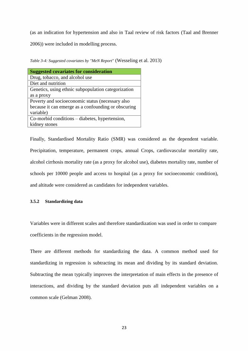
23
(as an indication for hypertension and also in Taal review of risk factors (Taal and Brenner
2006)) were included in modelling process.
Table 3-4: Suggested covariates by "MeN Report" (Wesseling et al. 2013)
Suggested covariates for consideration
Drug, tobacco, and alcohol use
Diet and nutrition
Genetics, using ethnic subpopulation categorization
as a proxy
Poverty and socioeconomic status (necessary also
because it can emerge as a confounding or obscuring
variable)
Co-morbid conditions – diabetes, hypertension,
kidney stones
Finally, Standardised Mortality Ratio (SMR) was considered as the dependent variable.
Precipitation, temperature, permanent crops, annual Crops, cardiovascular mortality rate,
alcohol cirrhosis mortality rate (as a proxy for alcohol use), diabetes mortality rate, number of
schools per 10000 people and access to hospital (as a proxy for socioeconomic condition),
and altitude were considered as candidates for independent variables.
3.5.2 Standardizing data
Variables were in different scales and therefore standardization was used in order to compare
coefficients in the regression model.
There are different methods for standardizing the data. A common method used for
standardizing in regression is subtracting its mean and dividing by its standard deviation.
Subtracting the mean typically improves the interpretation of main effects in the presence of
interactions, and dividing by the standard deviation puts all independent variables on a
common scale (Gelman 2008).

24
3.6 Geographically weighted regression (GWR)
GWR – as a method which provides detailed information about local areas – is increasingly
becoming more popular for regression analysis. GWR has a better description of the complex
interplay between the variables in local areas by providing a local form of linear regression.
The model constructs one equation for each feature by incorporating the independent
variables falling within the bandwidth of each target feature.
The model is fully described by Fothering et al. (Fotheringham et al. 2002). GWR extends the
concept of global regression model by adding regional parameters. Equation 8 descrobes the
model:
where:
(ui, vi): the location of point i in the space
β0 and βk : the coefficients
εi : the random error term at point i
β0 and βk are the parameters that should be estimated. To estimate these parameters, each
observation is weighted according to its distance to the target point i. In order to weight the
observations, Gaussian weighting kernel function is used (equation 9). The Gaussian kernel
curve is shown in figure 3-3. Closer observations get higher weights in the spatial context of
Gaussian kernel.
0 ( , ) ( , )i i i k i i ik i
k
y u v u v x Eq 8

25
where:
dij : distance between point i and j
b: bandwidth
Increasing the value of the bandwidth leads to the inclusion of more neighbouring data in the
local regression model result. A bandwidth value can be directly employed to the model
when we have some previous knowledge or experience about the likely effect of
neighbouring data. Otherwise, the Akaike Information Criterion (AIC) can estimate the
optimal bandwidth for the model. In this study, the latter was chosen.
Figure 3-3: Gaussin Kernel function (Fotheringham et al. 2002)
3.7 Multi criteria decision analysis (MCDA)
At this part of the study, it was decided to include expert’s knowledge about the risk factors
of CKD in order to know their opinions about the factors affecting CKD and identifying the
2
2exp( )
ij
ij
dw
b
Eq 9

26
importance of each factor in comparison with other factors, and finally create a risk map
according to the information received from the physicians to show which areas are more in
danger from the physicians’ perspective.
To this end, some approaches were needed to solve the problems related to decision support.
One approach, which is a principle of Multi Criteria Decision Analysis, is based on dividing
the decision problem into small, understandable parts and after analyzing each part combine
them in a logical manner (Malczewski 1999). MCDA can reveal the decision maker’s
preferences and GIS can provide techniques for analyzing MCDA problems. Accordingly,
these two distinct areas can complement each other (Malczewski 2006). Consequently, a
group of experts cordially invited to participate in this study to define and rank the possible
risk factors of CKD.
According to Eastman (Eastman) GIS based MCDA has five stages as below, which were
followed in this study as well.
1. selecting the criteria.
2. standardizing the factors (from 0-1 or 0-255).
3. determining the weight of each factor.
4. aggregating the criteria.
5. evaluating the result.
3.7.1 Criteria selection
Since it was not easy to gather all physicians together to decide on the possible risk factors of
CKD, the identification of the risk factors of CKD was performed by the two main physicians
who had a good knowledge of CKD in Costa Rica: Dr.Kristina Jakobsson, a senior consultant
and associate professor at Lund University, and Dr.Ineke Wesseling, a chairwoman of

27
Consortium for the Epidemic of Nephropathy in Central America and Mexico. So, the risk
factors of CKD were categorized into seven groups:
1. factors related to the general environment.
2. factors related to land use, especially agriculture.
3. factors related to the work environment.
4. socio economic and demographic factors (individual level).
5. socio economic and demographic factors (collective level).
6. life-style factors.
7. medical and related conditions.
However, we didn’t have access to all data related to each group. The available data only
covered the factors related to “general environment”, “socio economic and demographic
factors (individual level)” and “socio economic and demographic (collective level)” factors.
Consequently, according to the available data, the following criteria were used in this study:
Factors related to the general environment:
temperature
altitude
rainfall
housing proximity to crop land
Socio economic and demographic factors (individual level)
sex
age
Socioeconomic and demographic factors (collective level)
access to health care
social development index (SDI)
General environment include environmental factors that affect everyone living in the region.
Socio economic and demographic factors (individual level) are characteristics which can be
defined based on individual characteristics of all inhabitants in the area, however, only data
regarding to demographic factors were available in this study (the complete sub-factors can
be seen in appendix B). Socioeconomic and demographic factors (collective level) are

28
neighbourhood/area socioeconomic characteristics that are not made up of individual´s
data (like lack of access to different resources; a deprived neighbourhood).
The map for each criterion was created using the available data. In order to be able to overlay
all layers in GIS, all criteria maps were in raster with the cell size of 100 m* 100 m. Table 3-
5 shows the criteria maps created for each factor.
Table 3-5: Criteria maps used in MCDA
Criteria Criteria maps Temperature Temperature raster map
Altitude Digital Elevation Model
Rainfall Precipitation raster map
Proximity to crop land Distance map which shows the Euclidean distance from each point in the map
to the closest crop land
Sex Sex ratio map showing the No. Of man/No. Of Women in each district
Age Age ratio map showing the No. Of people aged above 60/No. Of people aged
below 60 in each district
Access to health care Distance map which shows the Euclidean distance from each point in the map
to the closest hospital
SDI Social development Index for each district
The temperature map was created using interpolation method from 24 weather stations. Each
weather station shows the average temperature from 1998 to 2002. Kriging as the spatial
analytical method was used to predict unknown values from average adjacent known values.
The precipitation map was created using 65 meteorological stations records as the average
yearly rainfall in 2008, and the kriging as an interpolation method was used. For creating
proximity to crop land and access to health care maps “Euclidean Distance” tool in ArcGIS is
used. This tool creates a raster map which shows the Euclidean distance from each point in
the map to the closest hospital. Age ratio and sex ratio and SDI were in district level.

29
3.7.2 Standardizing the factors
In order to be able to compare the values in the criteria map we need to transform them to a
comparable unit. There are different ways for standardizing the data such as linear scale
transformation, value/utility function approaches, probabilistic approaches and fuzzy
membership approaches (Malczewski 1999). In this study, a linear transformation as a most
commonly used technique in multi-criteria analysis is used for creating commensurate criteria
maps.
The value of standard maps can range from 0 to 1; the higher the score the higher the risk of
CKD incidence. According to the type of criteria, they should be maximised or minimised.
When the value is maximised high values get the higher score and when it is minimised high
values get the lower scores. For example, experts believe that there is positive correlation
between high temperature and CKD mortality rate, thus temperature should be maximised. In
other words, we should assign high scores (close to 1) to the high temperature and low scores
to the low temperature (close to 0). Transformation of maximised and minimised criteria can
be performed as equation 10 and 11 respectively (Malczewski 1999):
All the participants had the same opinion about the minimisation or maximisation of almost
all factors except for precipitation. For precipitation the opinion of the majority is considered.
min
'
max min
ij j
ij
j j
x xx
x x
max
'
max min
j ij
ij
j j
x xx
x x
Eq 10
Eq 11

30
According to the questionnaire, proximity to crops, altitude, precipitation and Social
Development Index were minimised and temperature, access to hospital, age ratio and sex
ratio were maximised.
3.7.3 Determining the weight of each factor
In order to weight each criteria map, Analytical Hierarchy Process (AHP) was used. AHP
was developed by Saaty (Malczewski 2006) and it involves pair wise comparisons. In this
method, a hierarchy structure is needed to represent the problem and pair wise comparison
should be built to show their relationships. Having selected the main criteria, sub criteria
were selected according to the level of dependency to the main criteria. The hierarchy
structure for this study is shown in figure 3-4.
Figure 3-4: MCDA Criteria and Sub Criteria
In each level, each pair of criteria should be compared and weighted from 1 to 9 according to
its influence on CKD. The scale to use when comparing each pair of criteria is shown in
Table 3-6.
CKD Susceptibility map
General Environment
Temperature
Altitude
Rainfall
Proximity to Crop land
Socioeconomic and demographic factors (individual level)
Age
Sex
Socioeconomic and demographic factors (Collective
level)
Access to Hospital
Social Development
Index

31
Table 3-6: Values for the experts for pair wise comparison of criteria
Choice Importance Value
Equally preferred 1 Moderately preferred 3
Strongly preferred 5
Very Strongly preferred 7
Extremely preferred 9
Values in between preferences 2, 4, 6, 8
A questionnaire was designed and sent to the physicians (see appendix B), the questionnaire
covered the whole seven criteria distinguished by the physicians. The questionnaire for
exploration of expert’s opinions was sent to 10 professionals. Among them, five experts
answered the questionnaire. So, the opinions of the 5 physicians were included in the result of
this study. For each factor tables was designed to perform a pair wise comparison. Figure 3-5
shows a sample table with regard to Socioeconomic and demographic (collective level)
factor.
9 8 7 6 5 4 3 2 1 2 3 4 5 6 7 8 9
1
Access
to
health
care
Social
development
index
Figure 3-5: pair wise comparison for Socioeconomic and demographic factors (collective level)
After receiving the whole results, a comparison matrix was constructed according to the
experts’ scores. Equation 12 shows the structure of comparison matrix for each criterion:
Equal Extreme Extreme

32
where : cij = 1/cji
3.7.4 Aggregating the criteria
To aggregate individual opinions the geometric mean (equation 13) was used as an efficient
model(Wu et al. 2008).
The weight for each criteria and sub criteria was calculated using the AHP tool created by
Thomas Pyzdek (Institute).
Saaty suggest calculating the Consistency Ratio (CR) to examine how the preferences of the
participant have been consistent. He suggests a maximum ratio of 0.1 is acceptable and when
the consistency ratio exceeds 0.1 re- examination is needed(Saaty 1987).
At the final stage a linear combination was used to combine all criteria and sub criteria
weights (equation 14).
where:
12 1
221
1 2
1
1
n
n
n n
c c
ccA
c c
12 1
1 1
21 2
1 1
1 2
1 1
1
1
km m
km m
n
k k
m mk k
m mn
aggregate k k
m mk k
m mn n
k k
c c
c cA
c c
i ic sc iF w w Sc
Eq12
Eq 13
Eq 14

33
Wci : weight of each Criteria
Wsci : weigh of sub critera
Sci : sub criteria values (map layers)
Having calculated the weights of each criteria and sub criteria using AHP analysis, the
corresponding weights were applied to the model using the formula in equation 14. The
combination of all criteria maps was performed by “Raster calculator” tool in ArcGIS.
3.7.5 Evaluating the result
In this study, Kappa statistics is used to evaluate if there is an agreement between physician’s
decisions and reality. The calculation is based on the difference between how much
agreement is actually observed compared to how much agreement would be expected to be
present by chance alone (Viera and Garrett 2005). The value of Kappa ranges from -1 to 1,
where 1 means 100% agreement and 0 is exactly what would be expected by chance and
negative values indicate agreement less than chance. The Kappa statistics was checked using
SPSS software.
1icw 1
iscw

34
4 RESULTS
Overall, 5821 individuals died from CKD over the study period from 1980 to 2012. Of them,
3585 (62%– 95% CI: 60% – 62%) were males and 2236 (38% – 95% CI: 37% – 39%) were
females (p < 0.05). The result showed that Canas county has the highest SMR (703.19 – 95%
CI: 701.33– 705.05), the highest mortality rate per 10000 people (22.2 – 95% CI: 17.07 –
28.9) in the period of 2008-2012 and also the highest mortality rate growth (Slope: 1.35 –
95% CI: 0.97 - 1.72) from 1980 to 2012.
The overall time trends of mortality rate, identification of hot spots and the procedures for
creating regression models are explained in details in the following subsections.
4.1 Time trends and hot spots
Figure 4-1 shows that, over the study period there was a significant increase in overall
mortality rate – from less than 3 in 1980 to more than 7 per 100000 populations in 2012. So
the relative risk shows about 3 times more risk of death due to CKD in 2012 compared to
1980 ( RR: 2.94 – 95% CI : 2.21 – 3. 89 ) .

35
Figure 4-1: CKD Mortality Rate per 100,000 people from 1980 to 2012
Figure 4-2 and 4-3 show higher slope of mortality rates over time in men compared to
women. The discrepancy are more visible when limiting the data to under 60-years of age
(females start with the mortality rate of around 1.5 and they have almost similar mortality rate
at the end of study period). This increase of mortality in younger males is in line with the
literature.
Figure 4-2: CKD Mortality Rate per 100,000 people according to gender from 1980 - 2012
y = 0.137x + 2.412R² = 0.849
0
1
2
3
4
5
6
7
8
Mortality Rate per 100000 (1980-2012)
y = 0.1941x - 381.76
y = 0.0812x - 158.29
0
1
2
3
4
5
6
7
8
9
10
1980 1985 1990 1995 2000 2005 2010
Mortality Rate per 100000 (Male vs. Female)
Male Death Rate per 100000 Female Death Rate Per 100000
Linear (Male Death Rate per 100000) Linear (Female Death Rate Per 100000)

36
Figure 4-3: Mortality Rate per 100, 000 people (under 60 years old)
Considering the mortality rate growth from 1980 to 2012, the slope of change was calculated
for each district. Figure 4-4 shows the slope of increase or decrease in mortality rate over the
study period. As figure 4-4 shows, northern counties have the highest CKD mortality rate
growth. The map also shows that there has been a decrease in CKD mortality rate over time
for noticeable parts of the central counties over the study period.
y = 0.0467x - 91.254
y = -0.0016x + 4.6688
0.00
0.50
1.00
1.50
2.00
2.50
3.00
3.50
4.00
1980 1985 1990 1995 2000 2005 2010
Mortality Rate per 100000 Under 60 years old ( Male vs. Female)
Male Death Rate per 100000 (Under 60 years old)
Female Death Rate per 100000 (Under 60 years old)
Linear (Male Death Rate per 100000 (Under 60 years old))
Linear (Female Death Rate per 100000 (Under 60 years old))

37
Figure 4-4: Mortality Rate Growth from 1980 to 2012 (Slope of change of the Mortality Rate)
Limiting the data to under 60 years old, the slope of change in mortality rate shows that there
is an increase in mortality rate in northern part of the country, compared to the central and
southern (figure 4-5).
Figure 4-5: Mortality Rate Growth from 1980 to 2012 for under 60 years old (Slope of change of the Mortality
Rate for under 60 years old)
N
N

38
SMR -a useful index for demonstrating the mortality rate adjusted by age and sex- is
calculated for each county of Costa Rica. An SMR of 100 indicates that CKD mortality rate
in the corresponding county is the same as the mortality rate of the whole country. The value
of SMR greater than 100 indicates there is a higher mortality rate in the corresponding county
than in Costa Rica, and the value less than 100 indicates there is a lower mortality rate in the
county than in Costa Rica.
Consequently, 5-yearly SMRs were calculated and mapped in figure 4-6. It can be seen that
the problem existed in a geographically limited area in northern part of the country in 1980s
and gradually spread to neighbouring areas in time; so that most of northern part are among
the highest SMR areas in the map of 2008-2012. In addition, for each 5-yearly period, the
SMR maps for people aged under 60 (figures 4-7 to 4-12) were also mapped and compared
with SMR of total population.
Visually, the maps of SMRs of total population and SMR of under 60 show almost the same
pattern in 1980s and the early 1990s (figure 4-7 to figure 4-9) except for the recent set of
maps in 2000 to 2012 (figure 4-10 to figure 4-12). In maps of 2008-2012, northern districts
have higher SMRs for the calculation of under 60 compared to the SMRs for the whole
population.

39
Figure 4-6: SMRs for 5-yearly intervals from 1983-2012

40
Figure 4-7: Standardized Mortality Ratio (1983 – 1987)
Figure 4-8: Standardized Mortality Ratio (1988 – 1992)

41
Figure 4-10: Standardized Mortality Ratio (1998 – 2002)
Figure 4-9: Standardized Mortality Ratio (1993 – 1997)

42
Figure 4-11: Standardized Mortality Ratio (2003 – 2007)
Figure 4-12: Standardized Mortality Ratio (2008 – 2012)

43
The cluster of high SMR values was demonstrated visually on figure 4-8 to figure 4-12.
However, spatially clustered counties should to be identified statistically. Consequently,
spatial auto correlation Global Moran’s I was applied to identify if there was a statistically
clustered pattern in the SMR values. In this study, the SMR of the whole population
calculated for the latest period (2008-2012) was selected for statistical analysis.
The result of the global Moran’I is shown in table 4-1. As it was explained in table 3-4, the
significant p value and positive z-score indicated that there was a cluster of high or low
values of SMR (2008 – 2012) in the dataset. Although global Moran’s I demonstrated there
was a cluster of mortalities in the dataset, cluster areas should be identified. Hotspot detection
was conducted using Anselin Local Moran’s I.
Table 4-1: Result of spatial autocorrelation (Global Moran’s I)
Moran’s Index 0.40
Z-score 6.82
p-value 0.00

44
Figure 4-13 shows the results of Anselin Local Moran’s I. According to the result, seven
counties identified as statistically significant cluster of high SMR values. These counties
included Bagaces, Canas, Carrillo, La Cruz, Liberia, Santa Cruz and Upala.
Figure 4-13: Anselin Local Moran's I map

45
4.2 Ordinary least squares and geographically weighted regression
The spatial relationship between CKD mortality cases and its risk factors can be determined
by implementing two of the common methods in geography, Geographically Weighted
Regression (GWR) and Ordinary Least Square (OLS). In global regression models such as
OLS, the results are unreliable when the relationships between dependent and independent
variables are inconsistent across the study area (i.e. regional variation or nonstationary). In
this study, both OLS and GWR models were examined to determine which method would
provide a better fit to the observation.
4.2.1 Model selection
SMR (2008 – 2012) was selected as a dependent variable. Cardiovascular mortality rate,
diabetes mortality rate , alcohol cirrhosis mortality rate , access to hospital , schools rate per
10000 people, temperature, permanent crops, annual crops, precipitation, and altitude were
selected as candidates for independent variables.
One of the assumptions in regression model is avoiding redundant variables, so we need to
determine which candidate on independent variables are highly correlated. A bivariate
correlation matrix was used to measure the strength and relationship between the variables by
measuring the correlation between two variables X and Y. A variable with high correlation
(more than 0.7) with others should be excluded from the analysis(Clark and Hosking 1986).
As can be seen in table 4-2, cardiovascular mortality rate, alcohol cirrhosis mortality rate and
school rate didn’t show a significant correlation with SMR (P > 0.05), so they should be
excluded from the independent variables. A high relationship can be seen between altitude
and temperature (r = - 0.73, p<0.05), so one of these variables should be excluded from the

46
independent variables as well. Since temperature shows a higher correlation with SMR,
altitude was excluded.
So, the final model incorporated 6 independent variables, of which four related to
environmental factors (Permanent crops, Annual crops, Precipitation, Temperature), one
related to traditional risk factor of CKD (Diabetes Mortality Rate), and one related to socio
economic factor (Access to hospital).

47
Table 4-2: a bivariate correlation matrix between all variables
Correlations
SMR AnnaulCrop PermanentC Precipitat Altitude temp AlchoholCir Diabetes SchoolRate CardioVasc AccessHosp
SMR
Pearson Correlation 1 .368** .410** -.268* -.367** .487** -.090 .415** -.094 .181 -.254*
Sig. (2-tailed) .001 .000 .016 .001 .000 .425 .000 .406 .106 .022
N 81 81 81 81 81 81 81 81 81 81 81
AnnaulCrop
Pearson Correlation .368** 1 .460** .122 -.549** .481** -.049 .284* -.065 .095 -.364**
Sig. (2-tailed) .001 .000 .277 .000 .000 .661 .010 .565 .400 .001
N 81 81 81 81 81 81 81 81 81 81 81
PermanentC
Pearson Correlation .410** .460** 1 .269* -.408** .429** .035 .244* .197 -.027 -.369**
Sig. (2-tailed) .000 .000 .015 .000 .000 .757 .028 .079 .809 .001
N 81 81 81 81 81 81 81 81 81 81 81
Precipitat
Pearson Correlation -.268* .122 .269* 1 -.190 .203 -.138 -.306** .014 -.316** -.415**
Sig. (2-tailed) .016 .277 .015 .090 .069 .220 .005 .901 .004 .000
N 81 81 81 81 81 81 81 81 81 81 81
Altitude
Pearson Correlation -.367** -.549** -.408** -.190 1 -.731** .283* -.340** .269* -.251* .492**
Sig. (2-tailed) .001 .000 .000 .090 .000 .010 .002 .015 .024 .000
N 81 81 81 81 81 81 81 81 81 81 81
temp
Pearson Correlation .487** .481** .429** .203 -.731** 1 -.255* .322** -.178 .168 -.652**
Sig. (2-tailed) .000 .000 .000 .069 .000 .021 .003 .111 .135 .000
N 81 81 81 81 81 81 81 81 81 81 81
RateMortAl
Pearson Correlation -.090 -.049 .035 -.138 .283* -.255* 1 .127 .837** -.360** .009
Sig. (2-tailed) .425 .661 .757 .220 .010 .021 .259 .000 .001 .936
N 81 81 81 81 81 81 81 81 81 81 81
RateMortDi Pearson Correlation .415** .284* .244* -.306** -.340** .322** .127 1 .060 .410** -.137
Sig. (2-tailed) .000 .010 .028 .005 .002 .003 .259 .593 .000 .223

48
N 81 81 81 81 81 81 81 81 81 81 81
SchoolRate
Pearson Correlation -.094 -.065 .197 .014 .269* -.178 .837** .060 1 -.458** -.072
Sig. (2-tailed) .406 .565 .079 .901 .015 .111 .000 .593 .000 .522
N 81 81 81 81 81 81 81 81 81 81 81
CardioVasc
Pearson Correlation .181 .095 -.027 -.316** -.251* .168 -.360** .410** -.458** 1 .119
Sig. (2-tailed) .106 .400 .809 .004 .024 .135 .001 .000 .000 .290
N 81 81 81 81 81 81 81 81 81 81 81
AccessHosp
Pearson Correlation -.254* -.364** -.369** -.415** .492** -.652** .009 -.137 -.072 .119 1
Sig. (2-tailed) .022 .001 .001 .000 .000 .000 .936 .223 .522 .290
N 81 81 81 81 81 81 81 81 81 81 81
**. Correlation is significant at the 0.01 level (2-tailed).
*. Correlation is significant at the 0.05 level (2-tailed).

49
4.2.2 OLS and GWR model results
The strength and direction of relationship between SMR and the independent variables are
shown in the table 4-3. The sign of the coefficients showed a negative correlation between
access to hospital and precipitation, implying inverse relationships between SMR and those
independent variables. In contrast, a positive correlation was found between permanent crops,
annual crops, temperature, and diabetes mortality rate.
Among the independent variables, the coefficients of access to hospital, diabetes mortality
rate and annual crops were not statistically significant meaning that they did not contribute
much to the model. However, the coefficient of precipitation, permanent crop and
temperature were significant at 0.05 level.
The summary of OLS regression with regard to the model fit and other statistical reports is
shown in table 4-4. The global model fit (OLS), gave R2 and adjusted R2 of 0.48 and 0.43
respectively. Thus, over 40% of variability in SMR could be explained by these variables
(permanent crops, annual crops, precipitation, temperature, diabetes mortality rate, and access
to hospital). All VIF values were less than 7.5, suggesting no variable was redundant. The
Joint Wald statistic values and its associated p-value (p<0.05) showed the model was
statistically significant. A significant p-value of BP statistic indicated independent variables
were inconsistent to the dependent variables, meaning that there was a regional variation
(nonstationay) between independent and dependent variable. The significance of Jarque-Bera
Statistic showed the residuals deviated from a normal theoretical distribution. Likewise, the
global Moran’I statistics was applied to examine the presence of spatial clustering in the
residuals. The result showed the residuals were clustered (Figure 4-14).

50
Table 4-3: coefficients of variables in the regression model
Table 4-4: summary of OLS regression result
Dependent Variable SMR2008_2012
Number of Observations 81
Multiple R-Squared 0.48
Adjusted R-Squared 0.43
Akaike's Information Criterion (AICc) 949.59
Probability
Joint Wald Statistic 34.93 0.000000*
Koenker (BP) Statistic 21.00 0.000005*
Jarque-Bera Statistic 111.64 0.000374*
Variable Coefficient Probability VIF
Intercept 121.46 0.000000* …..
Precipitation -45.76 0.000084* 1.53
Permanent crop 32.31 0.003619* 1.47
Temperature 37.04 0.005405* 2.1
DiabetesMortalityRate 7.08 0.504230 1.42
Annual crops 7.59 0.481845 1.44
AccesstoHospital -5.96 0.636212 2.05

51
Figure 4-14: Result of global Moran'I on standard residuals for OLS model
The result of global Moran’s I as well as Koenker BP statistics indicated the existence of
nonstationary and clustered residuals respectively. Sufficient evidence therefore existed for
resorting to GWR (Cardozo et al. 2012; Getis and Ord 1996).

52
Temperature, precipitation and permanent crops were the only statistically significant
variables which contribute more to the model, so these variables were considered as inputs in
the GWR model.
The adjusted R2 (Adjusted R2 = 0.65) obtained using GWR implied a considerable
improvement in the model fitness with respect to OLS model (Adjusted R2 = 0.43).
AICc ,an index for comparing two regression models, in GWR model is lower and it
decreased from 949.59 in OLS model to 909.7 in GWR model. The lower the AICc the better
the model.
Likewise, the analysis of the residuals of GWR model showed a random distribution of the
residuals which implied GWR was a better model comparing to OLS. The result of the
analysis of the residuals of GWR model using global Moran’I is shown in figure 4-15.
The comparison between GWR model and OLS model can be seen in table 4-5.
Table 4-5: Comparison between GWR and OLS model
GWR OLS
Adjusted R2 AICc Residuals Adjusted R2 AICc Residuals
0.65 909.7 Random 0.43 949.59 Clustered

53
Figure 4-15: Result of global Moran's I for residuals of GWR model
As it was explained in the method part of this study, GWR constructs one equation for each
feature by incorporating the independent variables falling within the bandwidth of each target
feature. Thus, each county has a separate regression model with different coefficients for
each independent variable. Figure 4-16 shows the variation of the coefficients for each
independent variable across the study area.

54
Figure 4-16: GWR coefficients for all independent variables, (a)Coefficients of GWR model for
temperature, (b) Coefficients of GWR model for precipitation,(c) Coefficients of GWR model for
precipitation
As can be seen in figure 4-16, the coefficients of GWR showed consistency in the effect of
permanent crops (the coefficients are positive all over the study area), but inconsistencies in
the effect of temperature and precipitation in different parts of the country since the
coefficients of precipitation and temperature could be positive or negative for different
locations. The effect of temperature is highly positive in the north unlike to precipitation
which is highly negative in the north. What is interesting in comparing the coefficients of all
three independent variables is that the effect of all three variables was dominant in the north.

55
4.3 Multi criteria decision analysis
The weight of each criteria and sub criteria derived from AHP analysis are shown in figure 4-
17. The consistency ratio for comparing three main criteria and general environment factors
were 0.03 and 0.01 respectively which was less than 0.1. The lowest weight was assigned to
general environment and the highest weight was assigned to socioeconomic and demographic
factors.
Figure 4-17: The weight for each criteria and sub criteria
The result of MCDA is shown in figure 4-18. The result assigned each unique value to each
cell of the output raster, the higher the value the higher the risk of CKD. According to the
weights that experts assigned to each criteria and sub criteria, central part of the country has
the lowest values/risk.
CKD Susceptibility map
General Environment
Temperature
Altitude
Rainfall
Proximity to Crop land
Socioeconomic and demographic factors
(individual level)
Age
Sex
Socioeconomic and demographic factors
(Collective level)
Social Development
Index
Access to Hospital
59.1%
19.9%
11%
10%
17%
45% 37%
65.75%
%
34.24%
52.08%
47.91%

56
Figure 4-18: Result of MCDA
In order to be able to compare the results of the MCDA to SMR, the maximum score of each
district was extracted and classified into three groups: high, medium and low risks.
Similarly, the reclassification was performed to the SMR values. Table 4-6 shows how the
classification was performed according to the values of each map. For classification of
MCDA score, a natural break technique was used to classify the result to low, medium and
high risk. The advantage of using this method is that the break point is set where there is a
relatively big difference in data values. With regard to SMR, the values more than 200 (the
counties with the mortality rate twice more than the national) were classified as high risk,
values below 100 were categorised as low risk and the values in between were classified as

57
medium risk. Figure 4-19 shows the comparison between SMR and MCDA maps classified
according to the risk level. In both maps central parts of the country was considered as the
low risk regions. More districts in the northern parts of the country were identified as high
risk in comparison with MCDA map.
Table 4-6: categorisation of SMR values and MCDA scores
MCDA SMR
Low risk 0.16-0.38 Low risk 0-100
Medium risk 0.38-0.47 Medium risk 100-200
High risk 0.47-0.62 High risk >200
Figure 4-19: Comparison between MCDA and SMR

58
Table 4-7: Cross tabulation and Kappa result
MCDA* SMR Crosstabulation
SMR
Total Low Meduim High
MCDA
Low Count 206 67 10 283
Meduim Count 85 35 22 142
High Count 27 11 9 47
Total
Count 318 113 41 472
Value Approx. Sig.
Kappa .087 .016
Table 4-7 compares the number of districts classified in low, medium or high risk in the
MCDA map with low, medium or high risk districts in the SMR map. The Kappa statistic
with associated p-value was also estimated (Kappa: 0.087, p<0.05) and showed in table 4-7.
For interpreting a Kappa value Landis and Koch (1977) gave table 4-8 (Landis and Koch
1977), so in this study the Kappa value of 0.087 showed a slight agreement between MCDA
result and reality.
Considering the high risk districts, according to table 4-7, nine districts were recognised as
high risk in both maps.
Table 4-8: Interpreting Kappa value
kappa < 0.01 0.01 - 0.20 0.21 - 0.40 0.41 - 0.60 0.61 - 0.80 0.81 - 1.00
Interpretation
Poor agreement
Slight agreement Fair
agreement
Moderate agreemen
t
Substantial agreement
Almost perfect
agreement
The decision makers assigned 17% of the weight to the general environment, which was the
lowest weight among the three main criteria. According to my findings in the regression

59
model, CKD showed a high association with the environmental factors, so I changed the
weight of the general environment to 50% and two other criteria to 25% to investigate
whether we could get a better result more closely to the reality.
The result can be seen in figure 4-20. Comparing the result of new created map with the SMR
map, we can see that central parts of the country still remained as low risk, in contrast to the
northern parts.
Figure 4-20: Comparison between MCDA and SMR (with “General Environment” as the highest
weight)

60
Table 4-9: Cross tabulation and Kappa result
MCDA(Envi) * SMR Crosstabulation
SMR
Total Low Meduim High
MCDA(Envi) Low Count 167 50 6 223
Medui
m
Count 102 40 10 152
High Count 49 23 25 97
Total Count 318 113 41 472
Value Approx. Sig.
Kappa .133 .000
Table 4-9 compares the number of districts classified in low, medium or high risk in a new
created map (i.e. weight of environment: 50%, other factors:25%) with the SMR map. The
Kappa increased to 0.13(p<0.05)which showed a better agreement with the reality in
comparison with the previous result (however it still showed a slight agreement), also the
number of districts which were distinguished as high risk in both maps approximately tripled
and reached to 25 districts.

61
5 DISCUSSION
This study – which is the first of its kind in Costa Rica – identified the hot spots of CKD and
suggests that northern parts of Costa Rica deserve further CKD investigations to see what
practical measures could better control CKD in those areas. Wesseling et al. (Wesseling et al.
2014) looked at geographical distribution of CKD mortality in Costa Rica and concluded that
Guanacaste is a heterogeneous CKD "hot spot". This is consistent with our findings of
geographical distribution. The results also confirmed the findings of previous studies that
men are affected significantly more than women by this CKD epidemic (Cerdas 2005).
The study also showed significant associations between CKD mortality rate and
environmental factors (temperature, permanent crops, and precipitation). These associations
provide further evidence in support of the link between the current CKD epidemic and
farming activities – in particular heat stress which has already been considered as a highly
likely contributing factor by experts (Wesseling et al. 2013). These new-emerging factors
have now been named in the literature as non-traditional risk factors against traditional risk
factors of CKD (Almaguer et al. 2014).
The inconsistencies of the effects of temperature and precipitation in the GWR model in
different locations is indicative that there should be another related causal factor (likely to be
heat stress) in the exposure-outcome pathway. The consistencies in the effect of permanent
crops in different parts of the country provide further evidence on the role of agricultural
occupation in CKD (Almaguer et al. 2014). VanDervot et al. (VanDervort et al. 2014)
concluded in their study that agricultural occupation is a risk factor in CKD. The association
between permanent crops and CKD mortality rate is in line with the findings of VanDervort
et al.

62
With respect to the last research objective, it was found that the expert’s knowledge about the
effect of the environmental factors to CKD in Costa Rica is probably not adequate. The
current study found that experts believe environmental factors have the lowest effect on the
CKD, due to assigning the lowest weight to it. After increasing the weight of the
environmental factors, an improvement in the Kappa value was detected. Moreover, the
model with the highest weight for the environmental factors could recognise the high risk
districts better which confirms the effect of environmental factors to CKD in Costa Rica. This
result is consistent with our findings in the regression model.
The findings of this study also provide objective evidence on the progressive nature of the
current CKD problem in Costa Rica (i.e. steady increase in mortality rates and three times
more risk of mortality in 2012 compared to 1980). Therefore, actions should be taken by
those in charge, otherwise the problem is likely to continue becoming worse.
Several limitations to this study should also be acknowledged. In this study, the data
regarding temperature, precipitation, annual crops and permanent crops go back to several
years ago; so that there was no overlap between the study period and the variables of
permanent crops and annual crops in the model. However, this is unlikely to affect the results
due to the very slow progress of CKD which is a matter of 10 years from the beginning to
end stage renal disease. Therefore, the exposure assessment of the risk factors could well look
back to several years ago. From the medical point of view, once kidneys have been damaged
due to exposure to risk factors, they may continue going downward for many years, even
long after the exposure which has caused the damage has gone. Moreover, we do not expect
significant variations over time for most of these variables (e.g. temperature).
Both in MCDA and regression model, all CKD risk factors recognised by the experts or
mentioned in the literature review were not considered in the models due to lack of data.

63
Consequently, the models need improvements since they didn’t cover the whole aspects of
CKD risk factors. However, in medical studies prediction has little role and it is more about
associations to identify risk factors. In other words, the purpose of studies of this kind is not
to predict how many people is going to die – but to find out which risk factors have been
contributing to the illness in order to take proper actions to slow down the disease process or
mortality rates. In this context, this study has been successful in providing further evidence
on the possible role of heat stress and agricultural work in CKD mortality in Costa Rica.
Moreover, biological systems are usually too complex to be fully predicted and therefore it is
not expected for medical models to provide high prediction of the situation – but it is
expected for physical models.
With regard to the AHP questionnaire, useful comments were obtained from the participants
concerning development of the questionnaire such as the questionnaire format or
including/excluding some risk factors.

64
6 CONCLUSIONS
With regard to the first three objectives, the result showed a significant increase in CKD
mortalities from 1980 to 2012. The results provide objective evidence on the progressive
nature of the current CKD problem in Costa Rica (i.e. steady increase in mortality rates and
three times more risk of mortality in 2012 compared to 1980). The results also confirmed the
findings of previous studies that young men are affected significantly by this CKD epidemic.
With regard to the objective four, mortality pattern of CKD, seven counties were identified as
“hot spot” of CKD mortalities. Further studies in these counties, in particular Canas, are
needed to find more evidence of causal factors of CKD in these areas. A field work in the hot
spot area is recommended for gathering reliable data in a village level.
Considering the associations between environmental factors and CKD, significant
associations were found between CKD mortality rate and temperature, permanent crops, and
precipitation. These associations provide further evidence in support of the link between the
current CKD epidemic with farming activities and heat stress. It should be mentioned that
these associations were between SMR of the last period (2008-2012) and environmental
factors. The definition of permanent crop in this study in unclear due to incomplete metadata.
It is recommended that associations between CKD with different cultivated plants (sugarcane,
coffee, etc.) will be investigated.
The results of this study need to be consulted with physicians who are experts in CKD and
familiar with the region. The overall opinion of the physicians participated in this study
showed they might have inadequate knowledge of environmental factors affecting CKD in
Costa Rica.

65
In particular, the findings of this study cover two specific aspects. One relates to the newly
emerging non-traditional risk factors for CKD (agricultural occupation, heat stress etc.)
against traditional risk factors (diabetes mellitus, high blood pressure etc.). The study showed
significant associations between CKD mortality and temperature, permanent crops, and
precipitation. These associations provide further evidence in support of the link between the
current CKD epidemic and farming activities (permanent crops) and heat stress (temperature
& precipitation).
The second aspect relates to policy implications. Indeed, the findings of this study provided
objective evidence on the progressive nature of the CKD problem in Costa Rica (i.e. steady
increase in mortality rates over the study period; so that there was three times more risk of
mortality in 2012 compared to 1980 as well as the geographically progressive nature of the
problem over the time shown on the SMR maps).The identified hot spots in the northern parts
of the country, in particular in Canas, warrants further investigations to see what practical
measures could better control CKD in those areas.
Figure 6-1 demonstrates the key geographical areas which require further attention for
intervention.

66
Geographic areas which require further attention for intervention
County with the highest number of Mortality from 2008 to 2012:
San Jose (115 people)
County with the highest CKD Mortality Rate (MR) per 10000 people (2008 to 2012):
Canas (22.2 – 95% CI: 17.07 – 28.9)
County with the highest growth in CKD Mortality (1980 to 2012):
Canas (Slope: 1.35 – 95% CI: 0.97 - 1.72)
County with the highest CKD Standard Mortality Ratio (SMR) from 2008 to 2012:
Canas (703.19 – 95% CI: 701.33– 705.05)
Bagaces, Canas, Carrillo, La Cruz, Liberia, Santa Cruz in Guanacaste province and
Upala in Alajuela province identified as hotspot areas.

67
Figure 6-1: Geographical areas for action and resource allocation
68
References
Akaike, H. 1985. Prediction and Entropy. In A Celebration of Statistics, eds. A. Atkinson, and S. Fienberg, 1-24 pp.: Springer New York.
Allison, P. D. 1999. Multiple regression: A primer. Pine Forge Press.
Almaguer, M., R. Herrera, and C. M. Orantes. 2014. Chronic kidney disease of unknown etiology in agricultural communities. MEDICC Rev, 16: 9-15.
Amato Dante, D. 2005. Prevalence of chronic kidney disease in an urban Mexican population. Kidney international. Supplement: 11-17.
Anselin, L. 1995. Local indicators of spatial association—LISA. Geographical analysis, 27: 93-115.
Athuraliya, N. T., T. D. Abeysekera, P. H. Amerasinghe, R. Kumarasiri, P. Bandara, U. Karunaratne, A. H. Milton, and A. L. Jones. 2011a. Uncertain etiologies of proteinuric-chronic kidney disease in rural Sri Lanka. Kidney International, 80: 1212-1221.
Athuraliya, N. T., T. D. Abeysekera, P. H. Amerasinghe, R. Kumarasiri, P. Bandara, U. Karunaratne, A. H. Milton, and A. L. Jones. 2011b. Uncertain etiologies of proteinuric-chronic kidney disease in rural Sri Lanka. Kidney Int, 80: 1212-1221. DOI: 10.1038/ki.2011.258
Athuraliya, T. N., D. T. Abeysekera, P. H. Amerasinghe, P. V. Kumarasiri, and V. Dissanayake. 2009. Prevalence of chronic kidney disease in two tertiary care hospitals: high proportion of cases with uncertain aetiology. Ceylon Med J, 54: 23-25.
Bank, T. W. 2014. The Wold Bank, Costa Rica Retrieved 08-Oct-2014, from. http://www.worldbank.org/en/country/costarica
Brooks, D. R., O. Ramirez-Rubio, and J. J. Amador. 2012. CKD in Central America: a hot issue. American Journal of Kidney Diseases, 59: 481-484.
Cardozo, O. D., J. C. García-Palomares, and J. Gutiérrez. 2012. Application of geographically weighted regression to the direct forecasting of transit ridership at station-level. Applied Geography, 34: 548-558.
Cerdas, M. 2005. Chronic kidney disease in Costa Rica. Kidney International, 68: S31-S33.
Chadban Steven, J. S. 2003. Prevalence of kidney damage in Australian adults: The AusDiab kidney study. Journal of the American Society of Nephrology, 14: 131-138.

69
Chandrajith, R., S. Nanayakkara, K. Itai, T. Aturaliya, C. Dissanayake, T. Abeysekera, K. Harada, T. Watanabe, et al. 2011. Chronic kidney diseases of uncertain etiology (CKDue) in Sri Lanka: geographic distribution and environmental implications. Environmental geochemistry and health, 33: 267-278.
Chen Jing, J. 2005. Prevalence of decreased kidney function in Chinese adults aged 35 to 74 years. Kidney International, 68: 2837-2845.
Choi, H. S. H. 2006. The prevalence and risk factors of microalbuminuria in normoglycemic, normotensive adults. Clinical nephrology, 65: 256-261.
Clark, W. A., and P. L. Hosking. 1986. Statistical methods for geographers. Wiley New York.
Coresh, J., B. C. Astor, T. Greene, G. Eknoyan, and A. S. Levey. 2003. Prevalence of chronic kidney disease and decreased kidney function in the adult US population: Third National Health and Nutrition Examination Survey. Am J Kidney Dis, 41: 1-12. DOI: 10.1053/ajkd.2003.50007
Crowe, J., C. Wesseling, B. R. Solano, M. P. Umaña, A. R. Ramírez, T. Kjellstrom, D. Morales, and M. Nilsson. 2013. Heat exposure in sugarcane harvesters in Costa Rica. American journal of industrial medicine, 56: 1157-1164.
Curtin, L. R., and R. J. Klein. 1995. Direct standardization (age-adjusted death rates). Healthy People 2000 Stat Notes: 1-10.
Eastman, J. R. Guide to GIS and Image Processing Volume 2.
El Minshawy, O. 2011. End-stage renal disease in the El-Minia Governorate, upper Egypt: an epidemiological study. Saudi J Kidney Dis Transpl, 22: 1048-1054.
ESRI. Retrieved 28/02 2015, from. http://resources.arcgis.com/en/help/main/10.1/index.html#//005p00000030000000
ESRI. Retrieved 2015, from. http://resources.arcgis.com/en/help/main/10.1/index.html#//005p0000000n000000
Fotheringham, A. S., C. Brunsdon, and M. Charlton. 2002. Geographically weighted regression : the analysis of spatially varying relationships. Chichester : Wiley , cop. 2002.
Garg Amit, X. A. 2005. Identifying individuals with a reduced GFR using ambulatory laboratory database surveillance. Journal of the American Society of Nephrology, 16: 1433-1439.

70
Gelman, A. 2008. Scaling regression inputs by dividing by two standard deviations. Statistics in medicine, 27: 2865-2873.
Getis, A., and J. K. Ord. 1996. Local spatial statistics: an overview. Spatial analysis: modelling in a GIS environment, 374.
Gorry, C. 2014. CKDu ravages the Salvadoran countryside. MEDICC Rev, 16: 5-8.
Graham, P. L., K. Mengersen, and A. P. Morton. 2003. Confidence limits for the ratio of two rates based on likelihood scores: non-iterative method. Stat Med, 22: 2071-2083. DOI: 10.1002/sim.1405
Gujarati, D. N., and D. C. Porter. 2009. Basic econometrics. Boston : McGrawHill, 2009
5. ed.
Hanafi-Bojd, A. A., H. Vatandoost, M. A. Oshaghi, Z. Charrahy, A. A. Haghdoost, G. Zamani, F. Abedi, M. M. Sedaghat, et al. 2012. Spatial analysis and mapping of malaria risk in an endemic area, south of Iran: A GIS based decision making for planning of control. Acta Tropica, 122: 132-137. DOI: http://dx.doi.org/10.1016/j.actatropica.2012.01.003
Hipp, J. A., and N. Chalise. 2015. Spatial analysis and correlates of county-level diabetes prevalence, 2009-2010. Prev Chronic Dis, 12: E08. DOI: 10.5888/pcd12.140404
Hsu Chih-Cheng, C. C. 2006. High prevalence and low awareness of CKD in Taiwan: a study on the relationship between serum creatinine and awareness from a nationally representative survey. American journal of kidney diseases : the official journal of the National Kidney Foundation, 48: 727-738.
Institute, P. Retrieved 0502 2015, from. http://www.sixsigmatraining.org/six-sigma-tools/ahp-spreadsheet.html
ISHIOKA, F., K. KURIHARA, H. SUITO, Y. HORIKAWA, and Y. ONO. 2007. Detection of hotspots for three-dimensional spatial data and its application to environmental pollution data. Journal of Environmental Science for Sustainable Society, 1: 15-24.
Jafar Tazeen, H. T. 2005. Serum creatinine as marker of kidney function in South Asians: a study of reduced GFR in adults in Pakistan. Journal of the American Society of Nephrology, 16: 1413-1419.
Jarque, C. M., and A. K. Bera. 1980. Efficient tests for normality, homoscedasticity and serial independence of regression residuals. Economics Letters, 6: 255-259. DOI: http://dx.doi.org/10.1016/0165-1765(80)90024-5

71
Kumar, V., A. K. Abbas, N. Fausto, and J. C. Aster. 2009. Robbins and Cotran Pathologic Basis of Disease, Professional Edition: Expert Consult-Online. Elsevier Health Sciences.
Landis, J. R., and G. G. Koch. 1977. The measurement of observer agreement for categorical data. Biometrics, 33: 159-174.
Levin, A., P. Stevens, R. Bilous, J. Coresh, A. De Francisco, P. De Jong, K. Griffith, B. Hemmelgarn, et al. 2013. KDIGO clinical practice guideline for the evaluation and management of chronic kidney disease. Chapter 1: Definition and classification of CKD. Kidney inter., Suppl, 3: 19-62.
Li, S., Z. Zhao, X. Miaomiao, and Y. Wang. 2010. Investigating spatial non-stationary and scale-dependent relationships between urban surface temperature and environmental factors using geographically weighted regression. Environmental Modelling & Software, 25: 1789-1800.
Lozano, R., M. Naghavi, K. Foreman, S. Lim, K. Shibuya, V. Aboyans, J. Abraham, T. Adair, et al. 2012. Global and regional mortality from 235 causes of death for 20 age groups in 1990 and 2010: a systematic analysis for the Global Burden of Disease Study 2010. Lancet, 380: 2095-2128. DOI: 10.1016/s0140-6736(12)61728-0
Magnason Ragnar, L. R. 2002. Prevalence and progression of CRF in Iceland: a population-based study. American journal of kidney diseases : the official journal of the National Kidney Foundation, 40: 955-963.
Malczewski, J. 1999. GIS and multicriteria decision analysis. New York [u.a.]: Wiley.
Malczewski, J. 2006. GIS‐based multicriteria decision analysis: a survey of the literature. International Journal of Geographical Information Science, 20: 703-726.
Miettinen, O., and M. Nurminen. 1985. Comparative analysis of two rates. Statistics in Medicine, 4: 213–226.
Mitchell, A. 2005. The ESRI Guide to GIS Analysis: Spatial Measurements and Statistics. Vol 2. Redlands. CA: ESRI Press.
Nanayakkara, S., T. Komiya, N. Ratnatunga, S. T. Senevirathna, K. H. Harada, T. Hitomi, G. Gobe, E. Muso, et al. 2012. Tubulointerstitial damage as the major pathological lesion in endemic chronic kidney disease among farmers in North Central Province of Sri Lanka. Environ Health Prev Med, 17: 213-221. DOI: 10.1007/s12199-011-0243-9
O'Donnell, J. K., M. Tobey, D. E. Weiner, L. A. Stevens, S. Johnson, P. Stringham, B. Cohen, and D. R. Brooks. 2011a. Prevalence of and risk factors for chronic kidney disease in rural Nicaragua. Nephrology Dialysis Transplantation, 26: 2798-2805.
72
O'Donnell, J. K., M. Tobey, D. E. Weiner, L. A. Stevens, S. Johnson, P. Stringham, B. Cohen, and D. R. Brooks. 2011b. Prevalence of and risk factors for chronic kidney disease in rural Nicaragua. Nephrol Dial Transplant, 26: 2798-2805. DOI: 10.1093/ndt/gfq385
Orantes, C. M., R. Herrera, M. Almaguer, E. G. Brizuela, C. E. Hernández, H. Bayarre, J. C. Amaya, D. J. Calero, et al. 2011. Chronic kidney disease and associated risk factors in the Bajo Lempa region of El Salvador: Nefrolempa study, 2009. MEDICC review, 13: 14-22.
Organization, W. H. 2015. Retrieved 1902 2015, from. http://www.who.int/classifications/icd/en/
Otero, A., A. de Francisco, P. Gayoso, and F. Garcia. 2010. Prevalence of chronic renal disease in Spain: results of the EPIRCE study. Nefrologia, 30: 78-86. DOI: 10.3265/Nefrologia.pre2009.Dic.5732
Oviasu, O. U. I. 2012. The spatial analysis of diagnosed Chronic Kidney Disease in Nigeria: A case study of Edo State. PhD Thesis University of Sheffield
Peraza, S., C. Wesseling, A. Aragon, R. Leiva, R. A. García-Trabanino, C. Torres, K. Jakobsson, C. G. Elinder, et al. 2012. Decreased kidney function among agricultural workers in El Salvador. American Journal of Kidney Diseases, 59: 531-540.
Rajabi, M., A. Mansourian, and A. Bazmani. 2012. Susceptibility mapping of visceral leishmaniasis based on fuzzy modelling and group decision-making methods. Geospat Health, 7: 37-50. DOI: 10.4081/gh.2012.103
Rajapurkar, M. M., G. T. John, A. L. Kirpalani, G. Abraham, S. K. Agarwal, A. F. Almeida, S. Gang, A. Gupta, et al. 2012a. What do we know about chronic kidney disease in India: first report of the Indian CKD registry. BMC nephrology, 13: 10.
Rajapurkar, M. M., G. T. John, A. L. Kirpalani, G. Abraham, S. K. Agarwal, A. F. Almeida, S. Gang, A. Gupta, et al. 2012b. What do we know about chronic kidney disease in India: first report of the Indian CKD registry. BMC Nephrol, 13: 10. DOI: 10.1186/1471-2369-13-10
Ramirez-Rubio, O., D. R. Brooks, J. J. Amador, J. S. Kaufman, D. E. Weiner, and M. K. Scammell. 2013. Chronic kidney disease in Nicaragua: a qualitative analysis of semi-structured interviews with physicians and pharmacists. BMC public health, 13: 350.
Rogerson, P. A. 2001. Spatial Patterns. Statistical Methods for Geography. SAGE Publications, Ltd. London, England: SAGE Publications, Ltd.
Ruiz, M. O., C. Tedesco, T. J. McTighe, C. Austin, and U. Kitron. 2004. Environmental and social determinants of human risk during a West Nile virus outbreak in the greater Chicago area, 2002. International Journal of Health Geographics, 3: 8.

73
Saaty, R. W. 1987. The analytic hierarchy process—what it is and how it is used. Mathematical Modelling, 9: 161-176.
Sanati, N. A., and M. Sanati. 2013. Growing interest in use of geographic information systems in health and healthcare research: a review of PubMed from 2003 to 2011. JRSM short reports, 4: 2042533313478810.
Sun, W., J. Gong, J. Zhou, Y. Zhao, J. Tan, A. N. Ibrahim, and Y. Zhou. 2015. A Spatial, Social and Environmental Study of Tuberculosis in China Using Statistical and GIS Technology. Int J Environ Res Public Health, 12: 1425-1448. DOI: 10.3390/ijerph120201425
Taal, M. W., and B. M. Brenner. 2006. Predicting initiation and progression of chronic kidney disease: Developing renal risk scores. Kidney Int, 70: 1694-1705. DOI: 10.1038/sj.ki.5001794
Tobler, W. R. 1970. A computer movie simulating urban growth in the Detroit region. Economic geography: 234-240.
Torres, C., A. Aragon, M. Gonzalez, I. Lopez, K. Jakobsson, C. G. Elinder, I. Lundberg, and C. Wesseling. 2010. Decreased kidney function of unknown cause in Nicaragua: a community-based survey. Am J Kidney Dis, 55: 485-496. DOI: 10.1053/j.ajkd.2009.12.012
VanDervort, D. R., D. L. López, C. M. Orantes, and D. S. Rodríguez. 2014. Spatial Distribution of Unspecified chronic kidney disease in El Salvador by Crop Area cultivated and ambient temperature. MEDICC review, 16: 32.
Vela, X. F., D. O. Henriquez, S. M. Zelaya, D. V. Granados, M. X. Hernandez, and C. M. Orantes. 2014. Chronic kidney disease and associated risk factors in two Salvadoran farming communities, 2012. MEDICC Rev, 16: 55-60.
Viera, A. J., and J. M. Garrett. 2005. Understanding interobserver agreement: the kappa statistic. Fam Med, 37: 360-363.
Viktorsdottir Olof, O. 2005. Prevalence of chronic kidney disease based on estimated glomerular filtration rate and proteinuria in Icelandic adults. Nephrology Dialysis Transplantation, 20: 1799-1807.
Wesseling, C., J. Crowe, C. Hogstedt, K. Jakobsson, R. Lucas, and D. Wegman, 2013. Mesoamerican nephropathy: report from the first international research workshop on men. Report 9968924067. [in Swedish, English summary]
Wesseling, C., B. van Wendel de Joode, J. Crowe, R. Rittner, and K. Jakobsson. 2014. 0204 Mesoamerican nephropathy in Costa Rica: Geographical distribution and time trends of

74
chronic kidney disease mortality between 1970 and 2012. Occup Environ Med, 71 Suppl 1: A27. DOI: 10.1136/oemed-2014-102362.83
Wijkström, J., R. Leiva, C.-G. Elinder, S. Leiva, Z. Trujillo, L. Trujillo, M. Söderberg, K. Hultenby, et al. 2013. Clinical and pathological characterization of Mesoamerican nephropathy: a new kidney disease in Central America. American Journal of Kidney Diseases, 62: 908-918.
Wu, W.-H., C.-t. Chiang, and C.-T. Lin. 2008. Comparing the aggregation methods in the analytic hierarchy process when uniform distribution. WSEAS Transactions on Business and Economics, 5: 74-80.
Zhang, C., L. Luo, W. Xu, and V. Ledwith. 2008. Use of local Moran's I and GIS to identify pollution hotspots of Pb in urban soils of Galway, Ireland. Science of the total environment, 398: 212-221.

75
Appendix A: SMR, Mortality Rate (MR) and crude number of
deaths
Table A-1: SMR and MR and total Number of death (2008-2012)
NCANTON SMR Lower95%CI Upper95%CI MR per 10000 Total No. of Death
ALAJUELA 93.37 93.17 93.57 3.00 85
ALFARO RUIZ 21.09 20.67 21.50 0.67 1
ATENAS 86.70 86.16 87.24 3.83 10
GRECIA 66.17 65.86 66.49 2.07 17
GUATUSO 159.74 158.55 160.92 4.27 7
LOS CHILES 159.64 158.53 160.75 3.87 8
NARANJO 126.02 125.46 126.59 4.19 19
OROTINA 73.30 72.65 73.94 2.66 5
PALMARES 35.32 35.01 35.63 1.31 5
POAS 155.35 154.53 156.16 4.47 14
SAN CARLOS 89.77 89.49 90.06 2.46 37
SAN MATEO 72.47 71.46 73.47 3.45 2
SAN RAMON 65.08 64.79 65.37 2.15 19
UPALA 179.07 178.26 179.88 5.21 19
VALVERDE VEGA 68.76 68.09 69.44 2.19 4
ALVARADO 130.29 129.15 131.43 3.65 5
CARTAGO 67.04 66.81 67.27 2.06 32
EL GUARCO 73.14 72.60 73.68 1.84 7
JIMENEZ 94.10 93.18 95.02 2.90 4
LA UNION 45.32 45.06 45.57 1.14 12
OREAMUNO 95.85 95.29 96.42 2.46 11
PARAISO 57.44 57.09 57.80 1.45 10
TURRIALBA 102.03 101.62 102.44 3.40 24
ABANGARES 163.22 162.21 164.23 5.95 10
BAGACES 458.31 456.62 460.01 14.71 28
CANAS 703.19 701.33 705.05 22.21 55
CARRILLO 338.45 337.34 339.55 11.94 36
HOJANCHA 156.29 154.76 157.82 6.06 4
LA CRUZ 425.12 423.30 426.94 12.10 21
LIBERIA 395.52 394.53 396.51 11.29 61
NANDAYURE 187.09 185.71 188.48 7.09 7
NICOYA 214.32 213.67 214.98 9.95 41
SANTA CRUZ 323.53 322.71 324.35 13.65 60
TILARAN 80.01 79.30 80.71 2.99 5
BARVA 149.32 148.61 150.03 4.35 17
BELEN 60.91 60.38 61.44 2.13 5
FLORES 155.23 154.26 156.19 5.68 10
HEREDIA 73.08 72.82 73.34 2.26 30
SAN ISIDRO 73.58 72.93 74.22 2.28 5
SAN PABLO 73.83 73.24 74.43 2.53 6
SAN RAFAEL 90.06 89.56 90.57 2.77 12
SANTA BARBARA 103.60 102.95 104.24 2.89 10
SANTO DOMINGO 91.42 90.92 91.92 3.47 13
SARAPIQUI 70.57 70.16 70.99 1.46 11
GUACIMO 151.46 150.76 152.16 3.78 18
LIMON 164.54 164.06 165.01 4.38 46

76
MATINA 98.09 97.51 98.67 2.33 11
POCOCI 89.24 88.93 89.55 2.12 32
SIQUIRRES 86.71 86.24 87.18 2.13 13
TALAMANCA 102.96 102.25 103.68 2.38 8
AGUIRRE 84.96 84.28 85.64 2.48 6
BUENOS AIRES 58.59 58.12 59.06 1.38 6
CORREDORES 96.97 96.37 97.57 3.05 10
COTO BRUS 103.94 103.29 104.58 2.83 10
ESPARZA 72.67 72.14 73.21 2.49 7
GARABITO 59.64 58.97 60.32 1.35 3
GOLFITO 155.58 154.79 156.36 5.01 15
MONTES DE ORO 76.62 75.87 77.37 3.03 4
OSA 145.77 144.87 146.68 4.72 10
PARRITA 0.00 0.00 0.00 0.00 0
PUNTARENAS 122.45 122.08 122.82 3.96 42
ACOSTA 42.70 42.22 43.19 1.55 3
ALAJUELITA 70.92 70.62 71.23 1.67 21
ASERRI 97.44 96.93 97.95 2.53 14
CURRIDABAT 81.13 80.76 81.51 2.48 18
DESAMPARADOS 66.37 66.19 66.55 1.88 55
DOTA 45.64 44.75 46.54 1.50 1
ESCAZU 53.69 53.37 54.01 1.81 11
GOICOECHEA 58.51 58.28 58.73 1.98 26
LEON CORTES 230.07 228.47 231.66 5.99 8
MONTES DE OCA 82.80 82.43 83.17 3.50 19
MORA 53.66 53.19 54.13 1.85 5
MORAVIA 42.58 42.28 42.87 1.46 8
PEREZ ZELEDON 82.70 82.41 82.99 2.37 31
PURISCAL 88.29 87.77 88.81 3.52 11
SAN JOSE 85.37 85.21 85.53 3.29 115
SANTA ANA 66.39 65.95 66.82 2.06 9
TARRAZU 42.72 42.13 43.32 1.21 2
TIBAS 135.34 134.86 135.81 5.02 31
TURRUBARES 130.74 128.93 132.56 4.31 2
VAZQUEZ DE CORONADO 107.20 106.76 107.63 2.83 23
Table A-2: SMR and MR and Total Number of death (2003 - 2007)
NCANTON SMR Lower95%C
I
Upper95%C
I
MR per
10000
Total No. of
Death
ALAJUELA 121.3
6 121.11 121.61 3.55 92
ALFARO RUIZ 80.06 79.16 80.97 2.31 3
ATENAS 59.82 59.34 60.30 2.41 6
GRECIA 139.2
8 138.78 139.78 3.98 30
GUATUSO 133.0
5 131.89 134.22 3.30 5
LOS CHILES 108.3
4 107.39 109.29 2.42 5
NARANJO 193.6 192.91 194.43 5.88 25

77
7
OROTINA 69.39 68.71 70.07 2.28 4
PALMARES 84.79 84.26 85.31 2.88 10
POAS 52.96 52.45 53.48 1.39 4
SAN CARLOS 72.69 72.41 72.97 1.83 26
SAN MATEO 39.88 39.10 40.66 1.75 1
SAN RAMON 82.88 82.51 83.24 2.50 20
UPALA 216.5
0 215.60 217.41 5.81 22
VALVERDE VEGA 136.8
4 135.83 137.85 3.95 7
ALVARADO 116.4
1 115.27 117.55 2.99 4
CARTAGO 114.8
7 114.54 115.20 3.21 47
EL GUARCO 70.53 69.96 71.09 1.63 6
JIMENEZ 75.02 74.17 75.86 2.11 3
LA UNION 64.82 64.48 65.16 1.48 14
OREAMUNO 79.21 78.66 79.76 1.86 8
PARAISO 76.38 75.92 76.83 1.77 11
TURRIALBA 133.6
8 133.20 134.17 4.07 29
ABANGARES 178.1
2 177.01 179.22 5.91 10
BAGACES 432.1
8 430.42 433.95 12.76 23
CANAS 514.1
8 512.52 515.84 14.82 37
CARRILLO 357.0
4 355.84 358.24 11.54 34
HOJANCHA 210.9
3 209.08 212.78 7.48 5
LA CRUZ 308.2
1 306.60 309.83 8.06 14
LIBERIA 312.1
3 311.18 313.07 8.12 42
NANDAYURE 85.91 84.94 86.88 2.97 3
NICOYA 121.4
4 120.94 121.95 5.17 22
SANTA CRUZ 310.6
3 309.79 311.48 11.99 52
TILARAN 150.5
2 149.54 151.50 5.13 9
BARVA 133.6
9 132.96 134.41 3.55 13
BELEN 84.81 84.13 85.49 2.70 6
FLORES 108.0
4 107.17 108.90 3.58 6
HEREDIA 88.89 88.58 89.21 2.49 30
SAN ISIDRO 165.6
8 164.59 166.76 4.65 9
SAN PABLO 98.30 97.57 99.03 3.06 7
SAN RAFAEL 77.96 77.45 78.47 2.18 9
SANTA BARBARA 120.0 119.35 120.84 3.06 10

78
9
SANTO DOMINGO 62.72 62.28 63.15 2.16 8
SARAPIQUI 34.61 34.27 34.95 0.66 4
GUACIMO 41.05 40.65 41.45 0.94 4
LIMON 110.8
7 110.45 111.29 2.70 27
MATINA 77.92 77.35 78.50 1.70 7
POCOCI 98.71 98.35 99.08 2.16 28
SIQUIRRES 53.21 52.82 53.61 1.20 7
TALAMANCA 91.80 91.07 92.54 1.96 6
AGUIRRE 65.34 64.69 65.98 1.75 4
BUENOS AIRES 43.31 42.89 43.74 0.94 4
CORREDORES 58.63 58.16 59.10 1.70 6
COTO BRUS 51.99 51.53 52.44 1.31 5
ESPARZA 180.2
5 179.34 181.16 5.62 15
GARABITO 30.14 29.54 30.73 0.63 1
GOLFITO 197.7
4 196.85 198.63 5.88 19
MONTES DE ORO 22.07 21.64 22.50 0.80 1
OSA 141.9
5 141.07 142.83 4.23 10
PARRITA 81.32 80.40 82.24 2.37 3
PUNTARENAS 104.7
5 104.40 105.11 3.10 33
ACOSTA 15.43 15.13 15.73 0.51 1
ALAJUELITA 77.41 77.03 77.79 1.66 16
ASERRI 94.74 94.21 95.28 2.24 12
CURRIDABAT 73.61 73.23 74.00 2.05 14
DESAMPARADOS 92.43 92.19 92.67 2.38 57
DOTA 49.30 48.33 50.26 1.48 1
ESCAZU 78.71 78.30 79.13 2.41 14
GOICOECHEA 77.24 76.96 77.51 2.36 30
LEON CORTES 65.42 64.51 66.32 1.56 2
MONTES DE OCA 117.1
3 116.66 117.60 4.48 24
MORA 37.97 37.54 38.40 1.20 3
MORAVIA 53.96 53.61 54.31 1.67 9
PEREZ ZELEDON 67.51 67.24 67.79 1.78 23
PURISCAL 70.79 70.30 71.28 2.59 8
SAN JOSE 80.76 80.60 80.93 2.82 94
SANTA ANA 44.09 43.70 44.47 1.25 5
TARRAZU 98.72 97.75 99.68 2.53 4
TIBAS 106.1
0 105.67 106.52 3.57 24
TURRUBARES 0.00 0.00 0.00 0.00 0
VAZQUEZ DE
CORONADO 59.81 59.44 60.18 1.43 10

79
Table A-3: SMR and MR and Total Number of death (1998 - 2002)
NCANTON SMR Lower95%C
I
Upper95%C
I
MR per
10000
Total No. of
Death
ALAJUELA 115.1
8 114.91 115.45 3.14 70
ALFARO RUIZ 67.96 67.02 68.90 1.84 2
ATENAS 95.22 94.56 95.88 3.56 8
GRECIA 86.52 86.08 86.96 2.30 15
GUATUSO 67.35 66.41 68.28 1.53 2
LOS CHILES 24.46 23.98 24.94 0.51 1
NARANJO 94.15 93.56 94.73 2.66 10
OROTINA 62.12 61.42 62.82 1.91 3
PALMARES 64.23 63.72 64.75 2.02 6
POAS 115.2
4 114.38 116.09 2.83 7
SAN CARLOS 135.1
0 134.68 135.52 3.15 40
SAN MATEO 46.48 45.57 47.39 1.87 1
SAN RAMON 62.97 62.62 63.33 1.77 12
UPALA 63.88 63.37 64.39 1.59 6
VALVERDE VEGA 67.69 66.93 68.46 1.85 3
ALVARADO 102.1
2 100.97 103.28 2.44 3
CARTAGO 95.33 95.00 95.65 2.50 33
EL GUARCO 166.1
2 165.18 167.06 3.55 12
JIMENEZ 81.10 80.18 82.02 2.14 3
LA UNION 64.19 63.81 64.57 1.37 11
OREAMUNO 127.8
3 127.07 128.58 2.82 11
PARAISO 105.9
1 105.31 106.51 2.29 12
TURRIALBA 61.58 61.23 61.93 1.75 12
ABANGARES 158.5
7 157.47 159.67 4.92 8
BAGACES 253.0
4 251.54 254.53 6.89 11
CANAS 480.7
0 479.01 482.39 12.88 31
CARRILLO 403.8
4 402.46 405.22 12.09 33
HOJANCHA 138.0
5 136.49 139.61 4.59 3
LA CRUZ 252.9
6 251.39 254.53 6.06 10
LIBERIA 404.8
8 403.71 406.05 9.85 46
NANDAYURE 309.8
9 307.97 311.81 10.02 10
NICOYA 138.7
1 138.14 139.28 5.45 23
SANTA CRUZ 309.1
5 308.25 310.05 11.02 45
TILARAN 71.29 70.59 71.99 2.24 4
BARVA 99.93 99.24 100.62 2.47 8

80
BELEN 67.79 67.13 68.46 2.02 4
FLORES 85.34 84.51 86.18 2.66 4
HEREDIA 113.7
1 113.31 114.11 2.98 31
SAN ISIDRO 47.15 46.50 47.80 1.25 2
SAN PABLO 115.9
2 115.06 116.78 3.36 7
SAN RAFAEL 82.26 81.69 82.83 2.15 8
SANTA BARBARA 129.4
5 128.60 130.29 3.08 9
SANTO DOMINGO 133.5
3 132.85 134.20 4.32 15
SARAPIQUI 24.94 24.59 25.28 0.44 2
GUACIMO 80.97 80.32 81.62 1.72 6
LIMON 152.2
7 151.74 152.81 3.45 31
MATINA 74.76 74.11 75.42 1.51 5
POCOCI 81.99 81.60 82.38 1.65 17
SIQUIRRES 135.6
2 134.93 136.31 2.86 15
TALAMANCA 118.0
1 117.07 118.96 2.32 6
AGUIRRE 60.09 59.41 60.77 1.49 3
BUENOS AIRES 61.44 60.90 61.98 1.25 5
CORREDORES 90.15 89.56 90.74 2.41 9
COTO BRUS 53.57 53.10 54.03 1.25 5
ESPARZA 42.82 42.33 43.30 1.25 3
GARABITO 49.97 48.99 50.95 0.96 1
GOLFITO 128.0
8 127.36 128.81 3.55 12
MONTES DE ORO 80.27 79.36 81.18 2.69 3
OSA 125.5
7 124.75 126.39 3.48 9
PARRITA 91.24 90.21 92.27 2.48 3
PUNTARENAS 92.36 92.01 92.72 2.54 26
ACOSTA 52.03 51.44 52.62 1.61 3
ALAJUELITA 99.64 99.11 100.16 1.99 14
ASERRI 64.12 63.65 64.60 1.42 7
CURRIDABAT 82.15 81.70 82.59 2.14 13
DESAMPARADOS 85.97 85.70 86.24 2.07 40
DOTA 54.59 53.52 55.66 1.53 1
ESCAZU 107.1
4 106.62 107.67 3.06 16
GOICOECHEA 100.5
1 100.17 100.85 2.89 34
LEON CORTES 114.7
6 113.46 116.05 2.56 3
MONTES DE OCA 115.6
9 115.19 116.18 4.16 21
MORA 31.34 30.90 31.77 0.92 2
MORAVIA 47.33 46.98 47.68 1.39 7
PEREZ ZELEDON 56.86 56.59 57.13 1.39 17
PURISCAL 30.10 29.76 30.44 1.02 3
SAN JOSE 83.43 83.25 83.60 2.74 85
SANTA ANA 65.97 65.44 66.50 1.74 6

81
TARRAZU 116.5
8 115.44 117.73 2.82 4
TIBAS 74.77 74.42 75.13 2.36 17
TURRUBARES 0.00 0.00 0.00 0.00 0
VAZQUEZ DE
CORONADO 80.03 79.53 80.52 1.80 10
TableA-4: SMR and MR and Total Number of death (1993 - 1997)
NCANTON SMR Lower95%C
I
Upper95%C
I
MR per
10000
Total No. of
Death
ALAJUELA 104.0
1 103.73 104.29 2.78 54
ALFARO RUIZ 197.1
1 195.39 198.84 5.25 5
ATENAS 43.94 43.44 44.44 1.46 3
GRECIA 61.60 61.19 62.00 1.59 9
GUATUSO 107.9
0 106.40 109.39 1.76 2
LOS CHILES 149.2
5 147.94 150.56 2.60 5
NARANJO 54.03 53.56 54.50 1.49 5
OROTINA 66.28 65.53 67.03 2.09 3
PALMARES 13.87 13.60 14.14 0.39 1
POAS 53.24 52.64 53.84 1.39 3
SAN CARLOS 85.25 84.88 85.62 1.74 20
SAN MATEO 50.29 49.30 51.27 1.95 1
SAN RAMON 70.21 69.80 70.63 1.87 11
UPALA 111.6
2 110.85 112.40 2.13 8
VALVERDE VEGA 54.89 54.13 55.65 1.35 2
ALVARADO 172.9
6 171.27 174.66 3.54 4
CARTAGO 126.1
8 125.76 126.59 2.88 35
EL GUARCO 121.8
7 120.97 122.77 2.24 7
JIMENEZ 0.00 0.00 0.00 0.00 0
LA UNION 125.6
6 125.07 126.26 2.43 17
OREAMUNO 184.7
8 183.77 185.78 3.65 13
PARAISO 75.62 75.06 76.18 1.59 7
TURRIALBA 97.97 97.47 98.47 2.29 15
ABANGARES 121.5
8 120.52 122.65 3.19 5
BAGACES 500.1
0 497.79 502.41 12.68 18
CANAS 361.4
5 359.86 363.03 8.54 20
CARRILLO 319.6 318.41 320.97 9.44 24

82
9
HOJANCHA 65.76 64.47 67.05 1.56 1
LA CRUZ 291.3
5 289.33 293.37 5.14 8
LIBERIA 275.9
4 274.87 277.00 6.22 26
NANDAYURE 0.00 0.00 0.00 0.00 0
NICOYA 125.0
9 124.45 125.72 3.56 15
SANTA CRUZ 209.7
6 208.94 210.58 6.41 25
TILARAN 88.85 87.97 89.72 2.18 4
BARVA 94.31 93.56 95.07 2.07 6
BELEN 97.32 96.47 98.18 2.81 5
FLORES 80.39 79.48 81.30 2.19 3
HEREDIA 123.8
3 123.39 124.27 3.23 30
SAN ISIDRO 119.6
5 118.48 120.83 2.92 4
SAN PABLO 155.7
6 154.52 157.01 3.14 6
SAN RAFAEL 167.0
8 166.13 168.02 3.51 12
SANTA BARBARA 169.6
9 168.64 170.74 3.82 10
SANTO DOMINGO 66.67 66.14 67.20 1.81 6
SARAPIQUI 73.93 73.21 74.66 1.13 4
GUACIMO 32.95 32.50 33.41 0.69 2
LIMON 156.3
7 155.80 156.95 3.47 28
MATINA 95.60 94.84 96.37 2.26 6
POCOCI 105.5
2 105.00 106.04 1.94 16
SIQUIRRES 41.55 41.14 41.96 0.85 4
TALAMANCA 93.54 92.63 94.46 1.81 4
AGUIRRE 83.10 82.16 84.04 1.69 3
BUENOS AIRES 77.16 76.48 77.83 1.30 5
CORREDORES 90.86 90.19 91.54 1.71 7
COTO BRUS 57.20 56.64 57.76 0.95 4
ESPARZA 67.61 66.94 68.27 1.85 4
GARABITO 148.5
0 146.44 150.56 2.95 2
GOLFITO 219.3
2 218.24 220.39 4.51 16
MONTES DE ORO 79.50 78.40 80.60 2.00 2
OSA 67.56 66.90 68.22 1.40 4
PARRITA 85.97 84.77 87.16 1.74 2
PUNTARENAS 86.94 86.56 87.32 1.99 20
ACOSTA 91.27 90.38 92.17 2.20 4
ALAJUELITA 109.1
6 108.54 109.78 2.22 12
ASERRI 74.49 73.94 75.04 1.52 7
CURRIDABAT 49.50 49.10 49.89 1.08 6
DESAMPARADOS 95.13 94.80 95.45 1.99 33
DOTA 131.8
5 130.02 133.68 3.20 2

83
ESCAZU 42.83 42.46 43.21 1.05 5
GOICOECHEA 110.2
3 109.84 110.61 2.81 31
LEON CORTES 0.00 0.00 0.00 0.00 0
MONTES DE OCA 87.41 86.92 87.91 2.46 12
MORA 74.72 73.99 75.45 2.11 4
MORAVIA 95.62 95.03 96.21 2.07 10
PEREZ ZELEDON 106.7
4 106.31 107.17 2.08 24
PURISCAL 151.5
4 150.68 152.40 4.22 12
SAN JOSE 92.45 92.24 92.65 2.72 81
SANTA ANA 97.33 96.61 98.05 2.34 7
TARRAZU 38.77 38.01 39.53 0.78 1
TIBAS 59.77 59.42 60.12 1.38 11
TURRUBARES 85.87 84.19 87.56 2.02 1
VAZQUEZ DE
CORONADO 68.50 67.99 69.00 1.57 7
Table A-5: SMR and MR and Total Number of death (1988 - 1992)
NCANTON SMR Lower95%C
I
Upper95%C
I
MR per
10000
Total No. of
Death
ALAJUELA 126.6
9 126.30 127.08 2.48 41
ALFARO RUIZ 61.47 60.27 62.68 1.19 1
ATENAS 0.00 0.00 0.00 0.00 0
GRECIA 76.20 75.64 76.77 1.45 7
GUATUSO 425.7
2 421.99 429.46 5.40 5
LOS CHILES 45.51 44.62 46.41 0.60 1
NARANJO 138.5
9 137.63 139.55 2.75 8
OROTINA 0.00 0.00 0.00 0.00 0
PALMARES 66.18 65.43 66.93 1.35 3
POAS 0.00 0.00 0.00 0.00 0
SAN CARLOS 79.45 79.00 79.90 1.22 12
SAN MATEO 0.00 0.00 0.00 0.00 0
SAN RAMON 82.51 81.94 83.08 1.60 8
UPALA 41.38 40.80 41.95 0.59 2
VALVERDE VEGA 42.53 41.70 43.37 0.76 1
ALVARADO 0.00 0.00 0.00 0.00 0
CARTAGO 96.60 96.16 97.05 1.67 18
EL GUARCO 180.9
2 179.58 182.27 2.57 7
JIMENEZ 0.00 0.00 0.00 0.00 0
LA UNION 103.6
0 102.92 104.28 1.55 9
OREAMUNO 63.27 62.55 63.98 0.97 3
PARAISO 87.01 86.25 87.77 1.38 5
TURRIALBA 105.4
6 104.84 106.08 1.83 11
ABANGARES 36.97 36.25 37.70 0.69 1

84
BAGACES 403.8
9 401.25 406.53 7.35 9
CANAS 301.1
5 299.37 302.93 5.16 11
CARRILLO 428.7
4 426.86 430.62 8.84 20
HOJANCHA 0.00 0.00 0.00 0.00 0
LA CRUZ 430.3
0 427.32 433.28 5.82 8
LIBERIA 285.8
7 284.51 287.23 4.76 17
NANDAYURE 111.3
2 109.77 112.86 2.05 2
NICOYA 109.1
1 108.40 109.82 2.23 9
SANTA CRUZ 154.1
3 153.25 155.00 3.35 12
TILARAN 128.7
2 127.46 129.98 2.29 4
BARVA 121.4
0 120.33 122.46 2.02 5
BELEN 124.2
0 122.98 125.42 2.59 4
FLORES 210.5
2 208.68 212.37 4.24 5
HEREDIA 126.5
1 125.94 127.08 2.46 19
SAN ISIDRO 144.6
5 143.01 146.29 2.65 3
SAN PABLO 77.61 76.53 78.68 1.23 2
SAN RAFAEL 62.57 61.86 63.28 1.01 3
SANTA BARBARA 79.93 79.02 80.83 1.34 3
SANTO DOMINGO 66.59 65.94 67.25 1.34 4
SARAPIQUI 30.29 29.70 30.89 0.37 1
GUACIMO 56.11 55.33 56.89 0.87 2
LIMON 139.0
8 138.40 139.76 2.34 16
MATINA 55.62 54.85 56.39 0.96 2
POCOCI 67.31 66.77 67.84 0.94 6
SIQUIRRES 98.39 97.60 99.18 1.51 6
TALAMANCA 274.9
4 272.91 276.98 4.07 7
AGUIRRE 125.5
2 124.10 126.95 1.93 3
BUENOS AIRES 66.97 66.21 67.73 0.86 3
CORREDORES 107.7
5 106.89 108.61 1.55 6
COTO BRUS 175.6
7 174.52 176.81 2.28 9
ESPARZA 0.00 0.00 0.00 0.00 0
GARABITO 0.00 0.00 0.00 0.00 0
GOLFITO 150.5
8 149.53 151.62 2.33 8
MONTES DE ORO 303.9
3 301.26 306.59 5.72 5
OSA 202.1
2 200.80 203.44 3.10 9

85
PARRITA 184.4
8 182.40 186.57 2.83 3
PUNTARENAS 83.25 82.80 83.70 1.43 13
ACOSTA 99.06 97.94 100.18 1.77 3
ALAJUELITA 90.27 89.54 90.99 1.41 6
ASERRI 127.1
7 126.29 128.05 1.96 8
CURRIDABAT 76.42 75.81 77.03 1.29 6
DESAMPARADOS 109.2
4 108.82 109.67 1.77 25
DOTA 0.00 0.00 0.00 0.00 0
ESCAZU 26.05 25.69 26.41 0.48 2
GOICOECHEA 126.9
1 126.40 127.42 2.42 24
LEON CORTES 68.12 66.79 69.46 1.04 1
MONTES DE OCA 93.88 93.27 94.50 1.97 9
MORA 91.82 90.79 92.86 1.88 3
MORAVIA 41.13 40.67 41.60 0.70 3
PEREZ ZELEDON 99.34 98.83 99.84 1.48 15
PURISCAL 56.05 55.42 56.69 1.13 3
SAN JOSE 100.0
0 99.75 100.25 2.18 61
SANTA ANA 109.6
5 108.69 110.61 1.97 5
TARRAZU 58.69 57.54 59.84 0.90 1
TIBAS 58.55 58.14 58.95 1.04 8
TURRUBARES 122.9
0 120.49 125.30 2.08 1
VAZQUEZ DE
CORONADO
100.3
6 99.56 101.17 1.73 6
Table A-6: SMR and MR and Total Number of death (1983 - 1987)
NCANTON SMR Lower95%CI Upper95%CI MortalityRate DthTot
ALAJUELA 105.38 104.96 105.80 1.70 24
ALFARO RUIZ 165.25 162.96 167.54 2.61 2
ATENAS 94.25 93.18 95.31 1.82 3
GRECIA 90.33 89.61 91.05 1.42 6
GUATUSO 129.97 127.42 132.52 1.33 1
LOS CHILES 139.79 137.85 141.73 1.54 2
NARANJO 70.94 70.14 71.74 1.16 3
OROTINA 95.88 94.55 97.21 1.74 2
PALMARES 90.73 89.70 91.76 1.53 3
POAS 41.35 40.54 42.16 0.65 1
SAN CARLOS 141.92 141.20 142.64 1.79 15
SAN MATEO 0.00 0.00 0.00 0.00 0
SAN RAMON 57.28 56.72 57.84 0.91 4
UPALA 118.59 117.42 119.75 1.38 4
VALVERDE VEGA 229.72 227.47 231.98 3.39 4
ALVARADO 0.00 0.00 0.00 0.00 0
CARTAGO 43.96 43.60 44.31 0.62 6
EL GUARCO 73.36 72.34 74.37 0.86 2
JIMENEZ 52.58 51.55 53.61 0.78 1

86
LA UNION 87.43 86.66 88.19 1.08 5
OREAMUNO 267.33 265.58 269.08 3.37 9
PARAISO 49.45 48.76 50.13 0.65 2
TURRIALBA 75.72 75.12 76.33 1.09 6
ABANGARES 96.54 95.21 97.88 1.47 2
BAGACES 482.38 479.03 485.72 7.27 8
CANAS 187.44 185.79 189.08 2.63 5
CARRILLO 497.49 495.13 499.86 8.36 17
HOJANCHA 0.00 0.00 0.00 0.00 0
LA CRUZ 228.39 225.81 230.98 2.51 3
LIBERIA 308.53 306.85 310.21 4.19 13
NANDAYURE 67.12 65.80 68.43 1.00 1
NICOYA 106.83 106.04 107.62 1.78 7
SANTA CRUZ 133.10 132.18 134.03 2.37 8
TILARAN 85.71 84.52 86.90 1.25 2
BARVA 34.48 33.81 35.16 0.47 1
BELEN 43.47 42.61 44.32 0.75 1
FLORES 120.12 118.46 121.79 1.99 2
HEREDIA 50.62 50.18 51.07 0.81 5
SAN ISIDRO 137.98 136.07 139.89 2.10 2
SAN PABLO 115.57 113.97 117.17 1.50 2
SAN RAFAEL 146.81 145.52 148.09 1.96 5
SANTA BARBARA 0.00 0.00 0.00 0.00 0
SANTO DOMINGO 114.27 113.27 115.27 1.88 5
SARAPIQUI 93.00 91.71 94.29 0.94 2
GUACIMO 0.00 0.00 0.00 0.00 0
LIMON 137.11 136.30 137.92 1.89 11
MATINA 84.35 83.18 85.52 1.21 2
POCOCI 34.67 34.19 35.15 0.40 2
SIQUIRRES 96.72 95.77 97.67 1.23 4
TALAMANCA 127.01 125.25 128.77 1.58 2
AGUIRRE 108.38 106.88 109.89 1.39 2
BUENOS AIRES 30.96 30.36 31.57 0.33 1
CORREDORES 131.59 130.43 132.74 1.58 5
COTO BRUS 26.79 26.27 27.32 0.29 1
ESPARZA 37.45 36.72 38.18 0.61 1
GARABITO 0.00 0.00 0.00 0.00 0
GOLFITO 146.29 145.12 147.46 1.88 6
MONTES DE ORO 0.00 0.00 0.00 0.00 0
OSA 55.73 54.95 56.50 0.71 2
PARRITA 75.43 73.95 76.91 0.96 1
PUNTARENAS 104.48 103.89 105.07 1.47 12
ACOSTA 83.83 82.67 84.99 1.25 2
ALAJUELITA 88.69 87.82 89.56 1.14 4
ASERRI 68.68 67.90 69.45 0.87 3
CURRIDABAT 99.48 98.61 100.35 1.37 5
DESAMPARADOS 124.11 123.56 124.65 1.66 20
DOTA 127.20 124.70 129.69 1.86 1
ESCAZU 126.07 125.13 127.00 1.91 7
GOICOECHEA 94.14 93.63 94.65 1.47 13
LEON CORTES 0.00 0.00 0.00 0.00 0
MONTES DE OCA 121.66 120.86 122.45 2.11 9

87
MORA 128.27 126.81 129.72 2.16 3
MORAVIA 97.33 96.48 98.18 1.35 5
PEREZ ZELEDON 72.24 71.74 72.74 0.88 8
PURISCAL 96.80 95.85 97.75 1.59 4
SAN JOSE 133.28 132.95 133.61 2.39 63
SANTA ANA 30.90 30.29 31.50 0.46 1
TARRAZU 80.87 79.28 82.45 1.03 1
TIBAS 74.56 74.01 75.12 1.08 7
TURRUBARES 0.00 0.00 0.00 0.00 0
VAZQUEZ DE
CORONADO 102.32 101.32 103.33 1.45 4

88
Appendix B: A sample of AHP Questionnaire
You are cordially invited to participate in a pilot study, for development of a questionnaire
which explores expert opinions on potential risk factors for CKD in Central America.
Such risk factors may be tangible or intangible, carefully measured or roughly estimated, well
or poorly understood—anything at all that might apply. By identification of the most
important tentative risk factors for CKD in Central America (note; CKD, not MeN or
CKDnT) future scientific studies as well as interventions can be better targeted.
We use an Analytic Hierarch Process (AHP) to identify and weight the risk factors. AHP is a
Multi-Criteria Decision making Method that helps the decision-makers facing a complex
problem with multiple conflicting and subjective criteria. The items in this questionnaire are
deliberately not very specific, but relate to broad areas of concern.Your requested task is to:
A: fill in the questionnaire (part 1- 9)
B: give your comments (part 10) as to clarity of instructions, important items that are left out
etc.
We hope that you can find time to answer the questionnaire before Jan 30, so that we can
produce a final questionnaire to be sent to all CENCAM members already in March. Results
will be presented at the 2nd International Workshop on MeN in Costa Rica, Nov 2015.
Further, the results of the pilot study will be used to produce a susceptibility map of CKD
mortality in Costa Rica, using geographical information systems (GIS) and available spatially
referenced data on potential risk factors, or indicators thereof.
Yours sincerely,
Ineke Wesseling
Chair, CENCAM board
Kristina Jakobsson
Div of Occupational and Environmental Medicine,
Lund University, Sweden
Ali Mansourian (responsible for analysis and reporting)

89
Dept of Physical Geography and Ecosystems Science (GIS Centre)
Lund University, Sweden
In the AHP method each pair of criteria should be compared and weighted from 1 to 9
according to your view its influence on CKD. If, for example, you are comparing factor J
with factor K and want to state that factor J is much more important than factor K then a
value of 7 (very strongly preferred) should be checked at the J side, or if you think two
factors are at the same level of importance you should check 1 (equally preferred) . The scale
to use when comparing each pair of criteria is shown in Table 1.
Table 0-1: Values for the experts for pair wise comparison of criteria
Choice Importance Value
Equally preferred 1
Moderately preferred 3
Strongly preferred 5
Very Strongly preferred 7
Extremely preferred 9
Values in between preferences 2, 4, 6, 8
In the present questionnaire factors associated with the incidence of Chronic Kidney Disease
(CKD) in Central America are tentatively be grouped as:
1. Factors in the general environment
2. Factors related to land use, especially agriculture
3. Factors related to the work environment
4. Socio economic and demographic factors (individual level)
5. Socio economic and demographic factors (collective level)
6. Life-style factors
7. Medical and related conditions
This questionnaire is designed to perform a pair wise comparison of the available factors
affecting the CKD, within each group, as follow:
1. Factors related to the general environment are:
Temperature
Altitude
Rainfall
Humidity
Drinking water quality
Air quality (particulate matter, PM)
Housing proximity to crop land

90
With regard to the factor “Air quality”, unlike the other factors, the association between this
factor and CKD has not been investigated yet. So if you think that this factor is not relevant,
please leave the comparisons which are between “Air quality” and other factors blank.
2. Factors related to land use are:
Type of agricultural organization
Pesticide use
3. Factors related to the work environment are:
Physical work load
Work environment temperature
Exposure to pesticides
Exposure to particles
Piece work
Informal employment (no formal contract, job insecurity, low income…)
4. Socioeconomic and demographic factors (individual level) are:
Sex
Age
Family income
Educational level
Migrant status
5. Socioeconomic and demographic factors (collective level) are:
Access to health care
Social development Index
6. Life-style factors are:
Tobacco smoking
Alcohol use
Use of illegal drugs
Obesity
Sugar intake
Water intake
7. Medical and other conditions are:
Metabolic syndrome and related diseases (diabetes, hypertension)
Genetic predisposition
Exposure to infectious diseases transmitted by rodents (leptospira, hantavirus and
others)
Regular use of pain-killers

91
Recurrent urinary tract infections
Use of nephrotoxic drugs and herbs
Your task: Please compare the relative importance of each pair of factors affecting the
Chronic Kidney Disease using the scale below:
Part 1: Comparison of factors related to general environment
9 8 7 6 5 4 3 2 1 2 3 4 5 6 7 8 9
1 Temperature Altitude
2 Temperature Humidity
3 Temperature Rainfall
4 Temperature
Drinking
water
quality
5 Humidity Altitude
6 Humidity Rainfall
7 Humidity
Drinking
water
quality
8 Rainfall Altitude
9 Rainfall
Drinking
water
quality
10
Drinking
water
quality Altitude
11
Air quality
(particulate
matter, PM) Temperature
Equal Extreme Extreme
Strong Strong

92
9 8 7 6 5 4 3 2 1 2 3 4 5 6 7 8 9
12
Air quality
(particulate
matter, PM) Altitude
13
Air quality
(particulate
matter, PM) Humidity
14
Air quality
(particulate
matter, PM) Rainfall
15
Air quality
(particulate
matter, PM)
Drinking
water
quality
16
Housing
proximity to
cropland Temperature
17
Housing
proximity to
cropland Altitude
18
Housing
proximity to
cropland Humidity
19
Housing
proximity to
cropland Rainfall
20
Housing
proximity to
cropland
Drinking
water
quality
21
Housing
proximity to
cropland Air quality
Part 2: Comparison of factors related to land use
9 8 7 6 5 4 3 2 1 2 3 4 5 6 7 8 9
1
Pesticide
use
Type of
agricultural
organization
Equal Extrem
e Extreme
Strong Strong
Equal Extreme Extreme
Strong Strong

93
Part 3: Comparison of factors related to the Work Environment
9 8 7 6 5 4 3 2 1 2 3 4 5 6 7 8 9
1 Physical work
load
Work
environment
temperature
2
Physical work
load Exposure to
pesticides
3
Physical work
load Exposure to
particles
4
Physical work
load Piece work
5
Physical work
load Informal
employment
6
Work
environment
temperature
Exposure to
pesticides
7
Work
environment
temperature
Exposure to
particles
8
Work
environment
temperature Piece work
9
Work
environment
temperature
Informal
employment
10
Exposure to
pesticides Exposure to
particles
11
Exposure to
pesticides Piece work
12
Exposure to
pesticides Informal
employment
13
Exposure to
particles Piece work
Equal Extreme Extreme
Strong Strong

94
9 8 7 6 5 4 3 2 1 2 3 4 5 6 7 8 9
14
Exposure to
particles Informal
employment
15 Piece work
Informal
employment
Part 4: Comparison of Socioeconomic and demographic factors (Individual level)
9 8 7 6 5 4 3 2 1 2 3 4 5 6 7 8 9
1 Age Sex
2 Age
Family
income
3 Age
Educational
level
4 Age
Migrant
status
5 Sex
Family
income
6 Sex
Educational
level
7 Sex
Migrant
status
8
Family
income Educational
level
Equal Extreme Extreme
Strong Strong
Equal Extrem
e Extreme
Strong Strong

95
9 8 7 6 5 4 3 2 1 2 3 4 5 6 7 8 9
9
Family
income Migrant
status
10
Educational
level Migrant
status
Part 5: Comparison of Socioeconomic and demographic factors (collective level)
9 8 7 6 5 4 3 2 1 2 3 4 5 6 7 8 9
1
Access to
health care
Social
development
index
Part 6: Comparison of life style factors
9 8 7 6 5 4 3 2 1 2 3 4 5 6 7 8 9
1 Tobacco
smoking
Alcohol use
2
Tobacco
smoking Use of illegal
drugs
3
Tobacco
smoking obesity
4
Tobacco
smoking Sugar intake
Equal Extreme Extreme
Strong Strong
Equal Extreme Extreme
Strong Strong
Equal Extreme Extreme
Strong Strong

96
9 8 7 6 5 4 3 2 1 2 3 4 5 6 7 8 9
5
Tobacco
smoking Water intake
6 Alcohol use
Use of illegal
drugs
7 Alcohol use obesity
8 Alcohol use Sugar intake
9 Alcohol use Water intake
10
Use of illegal
drugs obesity
11
Use of illegal
drugs Sugar intake
12
Use of illegal
drugs Water intake
13 obesity Sugar intake
Equal Extreme Extreme
Strong Strong

97
9 8 7 6 5 4 3 2 1 2 3 4 5 6 7 8 9
14 obesity Water intake
15 Sugar intake Water intake
Equal Extreme Extreme
Strong Strong

98
Part 7: Comparison of factors related to Medical and other conditions
9 8 7 6 5 4 3 2 1 2 3 4 5 6 7 8 9
1
Metabolic syndrome and
related diseases
(diabetes, hypertension)
Genetic predisposition
2
Metabolic syndrome and
related diseases
(diabetes, hypertension)
Exposure to infectious
diseases transmitted by
rodents (leptospira,
hantavirus and others)
3
Metabolic syndrome and
related diseases
(diabetes, hypertension) Regular use of pain-killers
4
Metabolic syndrome and
related diseases
(diabetes, hypertension)
Recurrent urinary tract
infections
5
Metabolic syndrome and
related diseases
(diabetes, hypertension)
Use of nephrotoxic drugs and
herbs
6 Genetic predisposition
Exposure to infectious
diseases transmitted by
rodents (leptospira,
hantavirus and others)
7 Genetic predisposition Regular use of pain-killers
Equal Extreme Extreme
Strong Strong

99
9 8 7 6 5 4 3 2 1 2 3 4 5 6 7 8 9
8 Genetic predisposition
Recurrent urinary tract
infections
9 Genetic predisposition
Use of nephrotoxic drugs and
herbs
10
Exposure to infectious
diseases transmitted by
rodents (leptospira,
hantavirus and others)
Regular use of pain-killers
11
Exposure to infectious
diseases transmitted by
rodents (leptospira,
hantavirus and others)
Recurrent urinary tract
infections
12
Exposure to infectious
diseases transmitted by
rodents (leptospira,
hantavirus and others)
Use of nephrotoxic drugs and
herbs
13
Regular use of pain-
killers Recurrent urinary tract
infections
14
Regular use of pain-
killers Use of nephrotoxic drugs and
herbs
15
Use of nephrotoxic drugs
and herbs Recurrent urinary tract
infections

100
Part 8: Which statement do you agree with regards to each factor?
General Environment
Temperature
People who are living in the high-temperature areas are more susceptible to CKD
People who are living in the low-temperature areas are more susceptible to CKD
Altitude (assumes there is no option for neither)?
People who are living in the high altitude are more susceptible to CKD
People who are living in the low altitude are more susceptible to CKD
Rainfall
People who are living in the areas with high precipitation are more susceptible to CKD
People who are living in the areas with low precipitation are more susceptible to CKD
Humidity
People who are living in high humidity are more susceptible to CKD
People who are living in low humidity are more susceptible to CKD
Drinking water quality
People who have insufficient water quality are more susceptible to CKD
People who have good water quality are more susceptible to CKD
Air quality (particulate matter, PM) (generic, not informed answer)
People who are living in the air quality with the high level of PM are more susceptible to CKD
People who are living in the air quality with the low level of PM are more susceptible to CKD
Housing proximity to crop land
People who are living close to cropland are more susceptible to CKD

101
People who are living far from the cropland are more susceptible to CKD
land use
Type of agricultural organization
People who are living in small-scale agricultural organization more susceptible to CKD
People who are living in Plantations/monoculture agricultural organization are more susceptible to CKD
Pesticide use
People who are living in areas with high exposure to pesticides are more susceptible to CKD
People who are living in areas with low exposure to pesticides are more susceptible to CKD
work environment (some of these should offer option of NEITHER)
Physical work load
People with high physical work load are more susceptible to CKD
People with low physical work load are more susceptible to CKD
Work environment temperature
People who are exposed to high temperature during the work are more susceptible to CKD
People who are exposed to low temperature during the work are more susceptible to CKD
Exposure to pesticides
People who are exposed to high amount of pesticides at their work environment
People who are exposed to low amount of pesticides at their work environment
Exposure to particles
People who are exposed to high amount of particles at their work environment are more susceptible to CKD
People who are exposed to low amount of particles at their work environment are more susceptible to CKD

102
Piece work
People who have a piece work job are more susceptible to CKD
People who don’t have a piece work job are more susceptible to CKD
Informal employment (no formal contract, no job insecurity, low income…)
People with informal employment job are more susceptible to CKD
People with formal employment are more susceptible to CKD
Socioeconomic and demographic factors (Individual)
Sex
Men are more susceptible to CKD
Women are more susceptible to CKD
Age
Young people are more susceptible to CKD
Elderly people are more susceptible to CKD
Family income
People with low family income
People with high family income
Educational level
People with low education level are more susceptible to CKD
People with high education level are more susceptible to CKD
Migrant status
Immigrants are more susceptible to CKD
Native people are more susceptible to CKD

103
Socioeconomic and demographic factors (Collective)
Social development Index
People living in low Social development index areas are more susceptible to CKD
People living in high Social development index areas are more susceptible to CKD
Access to health care
People who have a bad access to health care are more susceptible to CKD
People who have a good access to health care are more susceptible to CKD
Life-style (some answers Strong +; some really no difference)
Tobacco smoking
People who smoke tobacco are more susceptible to CKD
People who don’t smoke tobacco are more susceptible to CKD
Alcohol use
People with a high alcohol consumption are more susceptible to CKD
People with low alcohol consumption are more susceptible to CKD
Use of illegal drugs
People who use illegal drugs are more susceptible to CKD
People who don’t use illegal drugs are more susceptible to CKD
Obesity
People with obesity are more susceptible to CKD
People with no obesity are more susceptible to CKD
Sugar intake
People with high sugar intake are more susceptible to CKD

104
People with low sugar intake are more susceptible to CKD
Water intake
People with high water intake are more susceptible to CKD
People with low water intake are more susceptible to CKD
Medical and other conditions
Metabolic syndrome and related diseases (diabetes, hypertension)
People with metabolic syndrome and related diseases (diabetes, hypertension) are more susceptible to CKD
People with no metabolic syndrome and related diseases (diabetes, hypertension) are more susceptible to CKD
Genetic predisposition
People with genetic predisposition are more susceptible to CKD
People with no genetic predisposition are more susceptible to CKD
Exposure to infectious diseases transmitted by rodents (leptospira, hantavirus and others)
People who have been exposed to infectious diseases transmitted by rodents (leptospira, hantavirus and others) are
more susceptible to CKD
People who have not been exposed to infectious diseases transmitted by rodents (leptospira, hantavirus and others) are
more susceptible to CKD
Regular use of pain-killers
People who use pain killers regularly are more susceptible to CKD
People who don’t use pain killers regularly are more susceptible to CKD
Recurrent urinary tract infections
People who have recurrent urinary tract infections are more susceptible to CKD
People who don’t have recurrent urinary tract infections are more susceptible to CKD

105
Use of nephrotoxic drugs and herbs
People who use nephrotoxic drugs and herbs are more susceptible to CKD
People who don’t use nephrotoxic drugs and herbs are more susceptible to CKD
Part 9: comparison of all 7 factors
9 8 7 6 5 4 3 2 1 2 3 4 5 6 7 8 9
1 General
environment
Land use
2 General
environment
Work
environment
3 General
environment
Socioeconomic
and
demographic
(Individual)
4 General
environment Life-style
5 General
environment
Medical and
other
conditions
6 Land use
Work
environment
7 Land use
Socioeconomic
and
demographic
(Individual)
8 Land use Life-style
9 Land use
Medical and
other
conditions
10
Work
environment Socioeconomic
and
demographic

106
9 8 7 6 5 4 3 2 1 2 3 4 5 6 7 8 9
(Individual)
11
Work
environment Life-style
12
Work
environment
Medical and
other
conditions
13
Socioeconomic
and
demographic
(Individual)
Life-style
14
Socioeconomic
and
demographic
(Individual)
Medical and
other
conditions
15 Life-style
Medical and
other
conditions
16
Socioeconomic
and
demographic
(Collective)
Life-style
17
Socioeconomic
and
demographic
(Collective)
Medical and
other
conditions
18
Socioeconomic
and
demographic
(Collective)
Work
environment
19
Socioeconomic
and
demographic
(Collective)
Socioeconomic
and
demographic
(Individual)
20
Socioeconomic
and
demographic
(Collective)
General
environment

107
9 8 7 6 5 4 3 2 1 2 3 4 5 6 7 8 9
21
Socioeconomic
and
demographic
(Collective)
Land use

108
Part 10: Please, give your comments as to selection of groups and items – missing items, ambiguous
wording, ……
The aim of the study was Suggestions for improvement:
□ 1 Very difficult to understand
□ 2
□ 3 Choice 3
□ 4
□ 5 Very easy to understand
The instructions for the questionnaire were Suggestions for improvement:
□ 1 Very difficult to understand
□ 2 Choice 2 Offer option of no answer
□ 3
□ 4
□ 5 Very easy to understand
It took approximately ……… minutes to answer the pilot questionnaire
30 minutes but due to on-line and needing to check each box using the double click and
accept in Word. Not the best way. Interactive version would have been much easier
Comments on groups and items in the pilot questionnaire:
Some groups are fairly specific and others very general so choosing to rank along a continuum seemed
impossible at times – Do you want to offer option to leave blank?

109
Missing groups and items:
Other comments:

110
Appendix C: Proposed Priorities from “MesoAmerican
Nephropathy Report” for Exploring Hypotheses for Causes of
CKD of unknown origin in Central America.
Highly Likely, High Priority to Investigate Further
Heat stress and dehydration (including electrolyte imbalances)
Non-steroidal anti-inflammatory drugs (NSAIDS)
Possible, High Priority to Investigate Further
Arsenic
Fructose intake
Nephrotoxic medications, including homeopathic medications
Leptospirosis and other endemic infections
Possible, High Priority but Logistically Difficult at this Time
Genetic susceptibility and epigenetics
Low birth weight and other prenatal, perinatal, and childhood exposures that increase
susceptibility
Unlikely but strongly believed, Medium Priority to Investigate Further
Pesticides
Urinary tract diseases and sexually transmitted diseases (STDs)
Little Information, Medium Priority to Investigate Further
Calcium in drinking water, or water ‘hardness’
Medication contamination and use of homeopathic medicines and non-approved drugs

111
Unlikely, Low Priority for Further Investigation
Lead
Mercury
Cadmium
Uranium
Aristolochic acid

112
Series from Lund University
Department of Physical Geography and Ecosystem Science
Master Thesis in Geographical Information Science (LUMA-GIS)
1. Anthony Lawther: The application of GIS-based binary logistic regression for
slope failure susceptibility mapping in the Western Grampian Mountains,
Scotland. (2008).
2. Rickard Hansen: Daily mobility in Grenoble Metropolitan Region, France.
Applied GIS methods in time geographical research. (2008).
3. Emil Bayramov: Environmental monitoring of bio-restoration activities using
GIS and Remote Sensing. (2009).
4. Rafael Villarreal Pacheco: Applications of Geographic Information Systems
as an analytical and visualization tool for mass real estate valuation: a case
study of Fontibon District, Bogota, Columbia. (2009).
5. Siri Oestreich Waage: a case study of route solving for oversized transport:
The use of GIS functionalities in transport of transformers, as part of
maintaining a reliable power infrastructure (2010).
6. Edgar Pimiento: Shallow landslide susceptibility – Modelling and validation
(2010).
7. Martina Schäfer: Near real-time mapping of floodwater mosquito breeding
sites using aerial photographs (2010)
8. August Pieter van Waarden-Nagel: Land use evaluation to assess the outcome
of the programme of rehabilitation measures for the river Rhine in the
Netherlands (2010)
9. Samira Muhammad: Development and implementation of air quality data mart
for Ontario, Canada: A case study of air quality in Ontario using OLAP tool.
(2010)
10. Fredros Oketch Okumu: Using remotely sensed data to explore spatial and
temporal relationships between photosynthetic productivity of vegetation and
malaria transmission intensities in selected parts of Africa (2011)
11. Svajunas Plunge: Advanced decision support methods for solving diffuse
water pollution problems (2011)
12. Jonathan Higgins: Monitoring urban growth in greater Lagos: A case study
using GIS to monitor the urban growth of Lagos 1990 - 2008 and produce
future growth prospects for the city (2011).
13. Mårten Karlberg: Mobile Map Client API: Design and Implementation for
Android (2011).
14. Jeanette McBride: Mapping Chicago area urban tree canopy using color
infrared imagery (2011)
15. Andrew Farina: Exploring the relationship between land surface temperature
and vegetation abundance for urban heat island mitigation in Seville, Spain
(2011)

113
16. David Kanyari: Nairobi City Journey Planner An online and a Mobile
Application (2011)
17. Laura V. Drews: Multi-criteria GIS analysis for siting of small wind power
plants - A case study from Berlin (2012)
18. Qaisar Nadeem: Best living neighborhood in the city - A GIS based multi
criteria evaluation of ArRiyadh City (2012)
19. Ahmed Mohamed El Saeid Mustafa: Development of a photo voltaic building
rooftop integration analysis tool for GIS for Dokki District, Cairo, Egypt
(2012)
20. Daniel Patrick Taylor: Eastern Oyster Aquaculture: Estuarine Remediation via
Site Suitability and Spatially Explicit Carrying Capacity Modeling in
Virginia’s Chesapeake Bay (2013)
21. Angeleta Oveta Wilson: A Participatory GIS approach to unearthing
Manchester’s Cultural Heritage ‘gold mine’ (2013)
22. Ola Svensson: Visibility and Tholos Tombs in the Messenian Landscape: A
Comparative Case Study of the Pylian Hinterlands and the Soulima Valley
(2013)
23. Monika Ogden: Land use impact on water quality in two river systems in
South Africa (2013)
24. Stefan Rova: A GIS based approach assessing phosphorus load impact on Lake
Flaten in Salem, Sweden (2013)
25. Yann Buhot: Analysis of the history of landscape changes over a period of 200
years. How can we predict past landscape pattern scenario and the impact on
habitat diversity? (2013)
26. Christina Fotiou: Evaluating habitat suitability and spectral heterogeneity
models to predict weed species presence (2014)
27. Inese Linuza: Accuracy Assessment in Glacier Change Analysis (2014)
28. Agnieszka Griffin: Domestic energy consumption and social living standards: a
GIS analysis within the Greater London Authority area (2014)
29. Brynja Guðmundsdóttir Detection of potential arable land with remote sensing
and GIS - A Case Study for Kjósarhreppur (2014)
30. Oleksandr Nekrasov Processing of MODIS Vegetation Indices for analysis of
agricultural droughts in the southern Ukraine between the years 2000-2012
(2014)
31. Sarah Tressel Recommendations for a polar Earth science portal
in the context of Arctic Spatial Data Infrastructure (2014)
32. Caroline Gevaert Combining Hyperspectral UAV and Multispectral Formosat-
2 Imagery for Precision Agriculture Applications (2014).
33. Salem Jamal-Uddeen Using GeoTools to implement the multi-criteria
evaluation analysis - weighted linear combination model (2014)
34. Samanah Seyedi-Shandiz Schematic representation of geographical railway
network at the Swedish Transport Administration (2014)
35. Kazi Masel Ullah Urban Land-use planning using Geographical Information
System and analytical hierarchy process: case study Dhaka City (2014)

114
36. Alexia Chang-Wailing Spitteler. Development of a web application based on
MCDA and GIS for the decision support of river and floodplain rehabilitation
projects (2014)
37. Alessandro De Martino Geographic accessibility analysis and evaluation of
potential changes to the public transportation system in the City of Milan
(2014)
38. Alireza Mollasalehi GIS Based Modelling for Fuel Reduction Using
Controlled Burn in Australia. Case Study: Logan City, QLD (2015)
39. Negin A. Sanati Chronic Kidney Disease Mortality in Costa Rica;
Geographical Distribution, Spatial Analysis and Non-traditional Risk Factors
(2015)