Christopher F Baum - University of Birmingham · Using Stata for data management and reproducible...

Using Stata for data managementand reproducible research

Christopher F Baum

Boston College and DIW Berlin

Birmingham Business School, March 2013

Christopher F Baum (BC / DIW) Using Stata BBS 2013 1 / 96

Overview of the Stata environment Stata’s update facility

Stata’s update facility

One of Stata’s great strengths is that it can be updated over theInternet. Stata is actually a web browser, so it may contact Stata’s webserver and enquire whether there are more recent versions of eitherStata’s executable (the kernel) or the ado-files. This enables Stata’sdevelopers to distribute bug fixes, enhancements to existingcommands, and even entirely new commands during the lifetime of agiven major release (including ‘dot-releases’ such as Stata 12.1).

Updates during the life of the version you own are free. You need onlyhave a licensed copy of Stata and access to the Internet (which maybe by proxy server) to check for and, if desired, download the updates.


Overview of the Stata environment Extensibility

Extensibility of official Stata

An advantage of the command-line driven environment involvesextensibility: the continual expansion of Stata’s capabilities. Acommand, to Stata, is a verb instructing the program to perform someaction.

Commands may be “built in” commands—those elements sofrequently used that they have been coded into the “Stata kernel.” Arelatively small fraction of the total number of official Stata commandsare built in, but they are used very heavily.



The vast majority of Stata commands are written in Stata’s ownprogramming language–the “ado-file” language. If a command is notbuilt in to the Stata kernel, Stata searches for it along the adopath.Like the PATH in Unix, Linux or DOS, the adopath indicates theseveral directories in which an ado-file might be located. This impliesthat the “official” Stata commands are not limited to those coded intothe kernel. Try it out: give the adopath command in Stata.

If Stata’s developers tomorrow wrote a new command named “foobar”,they would make two files available on their web site: foobar.ado(the ado-file code) and foobar.sthlp (the associated help file). Bothare ordinary, readable ASCII text files. These files should be producedin a text editor, not a word processing program.



The importance of this program design goes far beyond the limits ofofficial Stata. Since the adopath includes both Stata directories andother directories on your hard disk (or on a server’s filesystem), youmay acquire new Stata commands from a number of web sites. TheStata Journal (SJ), a quarterly refereed journal, is the primary methodfor distributing user contributions. Between 1991 and 2001, the StataTechnical Bulletin played this role, and a complete set of issues of theSTB are available on line at the Stata website.

The SJ is a subscription publication (articles more than three years oldfreely downloadable), but the ado- and sthlp-files may be freelydownloaded from Stata’s web site. The Stata help commandaccesses help on all installed commands; the Stata command finditwill locate commands that have been documented in the STB and theSJ, and with one click you may install them in your version of Stata.Help for these commands will then be available in your own copy.



User extensibility: the SSC archive

But this is only the beginning. Stata users worldwide participate in theStatalist listserv, and when a user has written and documented a newgeneral-purpose command to extend Stata functionality, theyannounce it on the Statalist listserv (to which you may freelysubscribe: see Stata’s web site).

Since September 1997, all items posted to Statalist (over 1,300)have been placed in the Boston College Statistical SoftwareComponents (SSC) Archive in RePEc (Research Papers inEconomics), available from IDEAS (http://ideas.repec.org) andEconPapers (http://econpapers.repec.org).



Any component in the SSC archive may be readily inspected with aweb browser, using IDEAS’ or EconPapers’ search functions, and ifdesired you may install it with one command from the archive fromwithin Stata. For instance, if you know there is a module in the archivenamed mvsumm, you could use ssc describe mvsumm to learnmore about it, and ssc install mvsumm to install it if you wish.Anything in the archive can be accessed via Stata’s ssc command:thus ssc describe mvsumm will locate this module, and make itpossible to install it with one click.

Windows users should not attempt to download the materials from aweb browser; it won’t work.

Try it out: when you are connected to the Internet, typessc describe mvsummssc install mvsummhelp mvsumm



The command ssc new lists, in the Stata Viewer, all SSC packagesthat have been added or modified in the last month. You may click ontheir names for full details. The command ssc hot reports on themost popular packages on the SSC Archive.

The Stata command adoupdate checks to see whether all packagesyou have downloaded and installed from the SSC archive, the StataJournal, or other user-maintained net from... sites are up to date.adoupdate alone will provide a list of packages that have beenupdated. You may then use adoupdate, update to refresh yourcopies of those packages, or specify which packages are to beupdated.



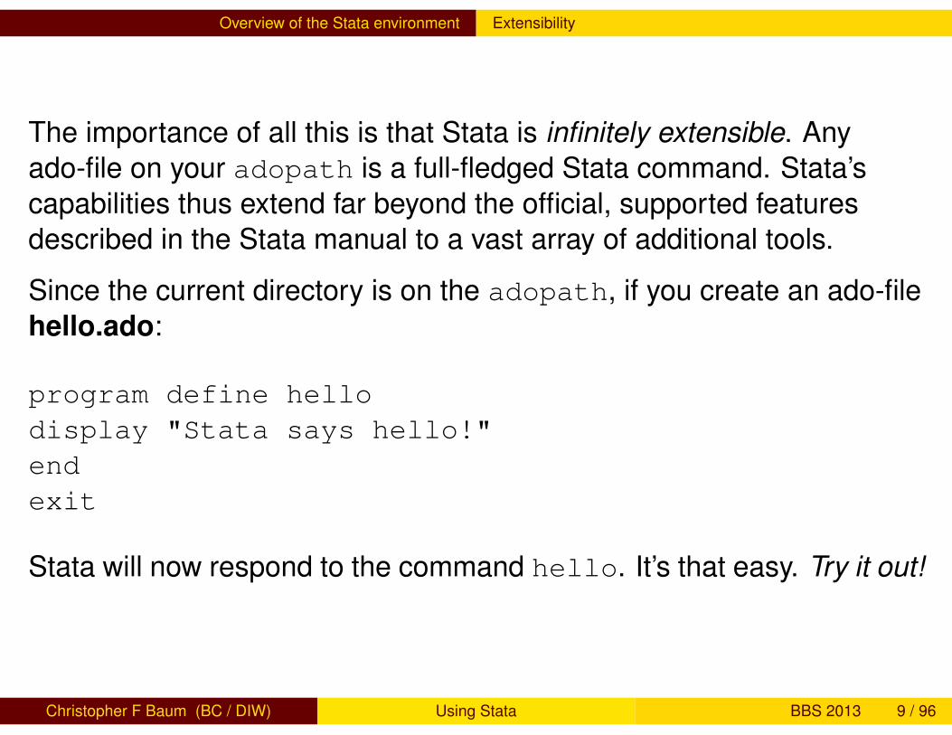
The importance of all this is that Stata is infinitely extensible. Anyado-file on your adopath is a full-fledged Stata command. Stata’scapabilities thus extend far beyond the official, supported featuresdescribed in the Stata manual to a vast array of additional tools.

Since the current directory is on the adopath, if you create an ado-filehello.ado:

program define hellodisplay "Stata says hello!"endexit

Stata will now respond to the command hello. It’s that easy. Try it out!


Working with the command line Stata command syntax

Stata command syntax

Let us consider the form of Stata commands. One of Stata’s greatstrengths, compared with many statistical packages, is that itscommand syntax follows strict rules: in grammatical terms, there areno irregular verbs. This implies that when you have learned the way afew key commands work, you will be able to use many more withoutextensive study of the manual or even on-line help.

The fundamental syntax of all Stata commands follows a template. Notall elements of the template are used by all commands, and someelements are only valid for certain commands. But where an elementappears, it will appear in the same place, following the same grammar.

Like Unix or Linux, Stata is case sensitive. Commands must be givenin lower case. For best results, keep all variable names in lower caseto avoid confusion.


Working with the command line Command template

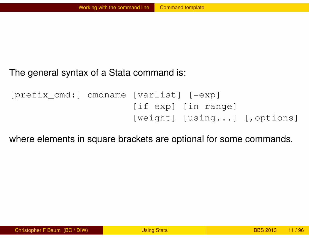
The general syntax of a Stata command is:

[prefix_cmd:] cmdname [varlist] [=exp][if exp] [in range][weight] [using...] [,options]

where elements in square brackets are optional for some commands.


Working with the command line Programmability of tasks

Programmability of tasks

Stata may be used in an interactive mode, and those learning thepackage may wish to make use of the menu system. But when youexecute a command from a pull-down menu, it records the commandthat you could have typed in the Review window, and thus you maylearn that with experience you could type that command (or modify itand resubmit it) more quickly than by use of the menus.

Stata makes reproducibility very easy through a log facility, the abilityto generate a command log (containing only the commands you haveentered), and the do-file editor which allows you to easily enter,execute and save sequences of commands, or program fragments.



Going one step further, if you use the do-file editor to create asequence of commands, you may save that do-file and reuse ittomorrow, or use it as the starting point for a similar set of datamanagement or statistical operations. Working in this way promotesreproducibility, which makes it very easy to perform an alternateanalysis of a particular model. Even if many steps have been takensince the basic model was specified, it is easy to go back and producea variation on the analysis if all the work is represented by a series ofprograms.

One of the implications of the concern for reproducible work: avoidaltering data in a non-auditable environment such as a spreadsheet.Rather, you should transfer external data into the Stata environment asearly as possible in the process of analysis, and only make permanentchanges to the data with do-files that can give you an audit trail ofevery change made to the data.



Programmable tasks are supported by prefix commands, as we willsoon discuss, that provide implicit loops, as well as explicit loopingconstructs such as the forvalues and foreach commands.

To use these commands you must understand Stata’s concepts oflocal and global macros. Note that the term macro in Stata bears noresemblance to the concept of an Excel macro. A macro, in Stata, isan alias to an object, which may be a number or string.


Working with the command line Local macros and scalars

Local macros and scalars

In programming terms, local macros and scalars are the “variables” ofStata programs (not to be confused with the variables of the data set).The distinction: a local macro can contain a string, while a scalar cancontain a single number (at maximum precision). You should use theseconstructs whenever possible to avoid creating variables with constantvalues merely for the storage of those constants. This is particularlyimportant when working with large data sets.

When you want to work with a scalar object—such as a counter in aforeach or forvalues command—it will involve defining andaccessing a local macro. As we will see, all Stata commands thatcompute results or estimates generate one or more objects to holdthose items, which are saved as numeric scalars, local macros (stringsor numbers) or numeric matrices.


Working with the command line Local macros and scalars

The local macro

The local macro is an invaluable tool for do-file authors. A local macrois created with the local statement, which serves to name the macroand provide its content. When you next refer to the macro, you extractits value by dereferencing it, using the backtick (‘) and apostrophe (’)on its left and right:

local george 2local paul = ‘george’ + 2

In this case, I use an equals sign in the second local statement as Iwant to evaluate the right-hand side, as an arithmetic expression, andstore it in the macro paul. If I did not use the equals sign in thiscontext, the macro paul would contain the string 2 + 2.


Working with the command line forvalues and foreach

forvalues and foreach

In other cases, you want to redefine the macro, not evaluate it, and youshould not use an equals sign. You merely want to take the contents ofthe macro (a character string) and alter that string. The two keyprogramming constructs for repetition, forvalues and foreach,make use of local macros as their “counter”. For instance:

forvalues i=1/10 {summarize PRweek‘i’

}

Note that the value of the local macro i is used within the body of theloop when that counter is to be referenced. Any Stata numlist mayappear in the forvalues statement. Note also the curly braces,which must appear at the end of their lines.



In many cases, the forvalues command will allow you to substituteexplicit statements with a single loop construct. By modifying the rangeand body of the loop, you can easily rewrite your do-file to handle adifferent case.

The foreach command is even more useful. It defines an iterationover any one of a number of lists:

the contents of a varlist (list of existing variables)the contents of a newlist (list of new variables)the contents of a numlist (list of integers)the separate words of a macrothe elements of an arbitrary list



For example, we might want to summarize each of these variables’detailed statistics from this World Bank data set:

sysuse lifeexpforeach v of varlist popgrowth lexp gnppc {

summarize ‘v’, detail}

Or, run a regression on variables for each region, and graph the dataand fitted line:

levelsof region, local(regid)foreach c of local regid {local rr : label region ‘c’

regress lexp gnppc if region ==‘c’twoway (scatter lexp gnppc if region ==‘c’) ///

(lfit lexp gnppc if region ==‘c’, ///ti(Region: ‘rr’) name(fig‘c’, replace))

}



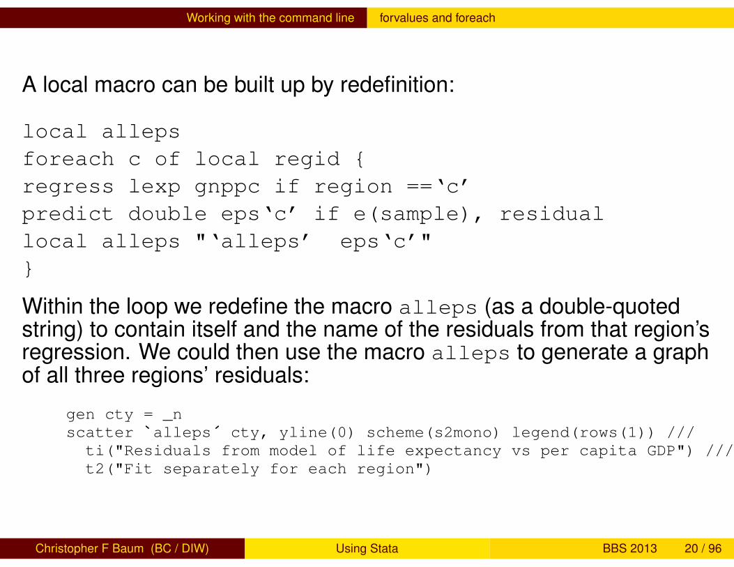
A local macro can be built up by redefinition:

local allepsforeach c of local regid {regress lexp gnppc if region ==‘c’predict double eps‘c’ if e(sample), residuallocal alleps "‘alleps’ eps‘c’"}

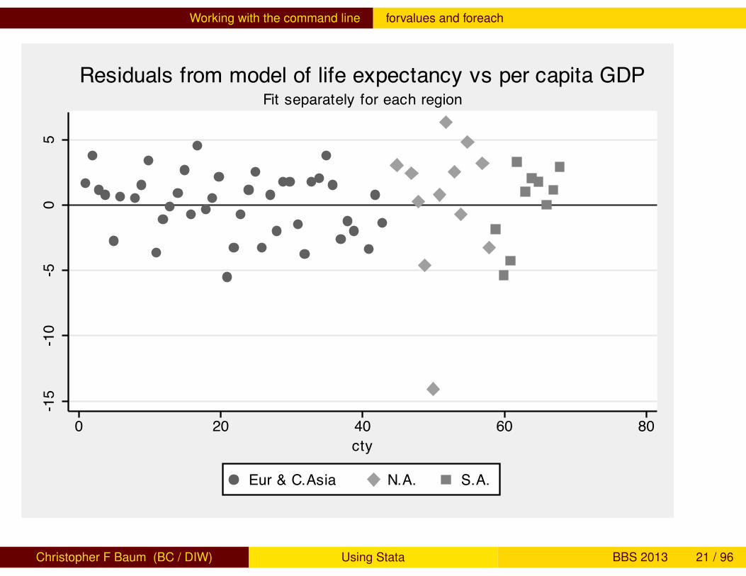
Within the loop we redefine the macro alleps (as a double-quotedstring) to contain itself and the name of the residuals from that region’sregression. We could then use the macro alleps to generate a graphof all three regions’ residuals:

gen cty = _nscatter `alleps´ cty, yline(0) scheme(s2mono) legend(rows(1)) ///ti("Residuals from model of life expectancy vs per capita GDP") ///t2("Fit separately for each region")



-15

-10

-50

5

0 20 40 60 80cty

Eur & C.Asia N.A. S.A.

Fit separately for each regionResiduals from model of life expectancy vs per capita GDP



Global macros

Stata also supports global macros, which are referenced by a differentsyntax ($country rather than ‘country’). Global macros are usefulwhen particular definitions (e.g., the default working directory for aparticular project) are to be referenced in several do-files that are to beexecuted. However, the creation of persistent objects of global scopecan be dangerous, as global macro definitions are retained for theentire Stata session. One of the advantages of local macros is thatthey disappear when the do-file or ado-file in which they are definedfinishes execution.


Working with the command line Prefix commands

Prefix commands

A number of Stata commands can be used as prefix commands,preceding a Stata command and modifying its behavior. The mostcommonly employed is the by prefix, which repeats a command over aset of categories. The statsby: prefix repeats the command, butcollects statistics from each category. The rolling: prefix runs thecommand on moving subsets of the data (usually time series).

Several other command prefixes: simulate:, which simulates astatistical model; bootstrap:, allowing the computation of bootstrapstatistics from resampled data; and jackknife:, which runs a commandover jackknife subsets of the data. The svy: prefix can be used withmany statistical commands to allow for survey sample design.


Data management: principles of organization and transformation The by prefix

The by prefix

You can often save time and effort by using the by prefix. When acommand is prefixed with a bylist, it is performed repeatedly for eachelement of the variable or variables in that list, each of which must becategorical. You may try it out:

sysuse census

by region: summ pop medage

will provide descriptive statistics for each of four US Census regions. Ifthe data are not already sorted by the bylist variables, the prefixbysort should be used. The option ,total will add the overallsummary.



This can be extended to include more than one by-variable:

generate large = (pop > 5000000) & !mi(pop)bysort region large: summ popurban death

This is a very handy tool, which often replaces explicit loops that mustbe used in other programs to achieve the same end.

The by-group logic will work properly even when some of the definedgroups have no observations. However, its limitation is that it can onlyexecute a single command for each category. If you want to estimate aregression for each group and save the residuals or predicted values,you must use an explicit loop.



The by prefix should not be confused with the by option available onsome commands, which allows for specification of a grouping variable:for instance

ttest price, by(foreign)

will run a t-test for the difference of sample means across domesticand foreign cars.

Another useful aspect of by is the way in which it modifies themeanings of the observation number symbol. Usually _n refers to thecurrent observation number, which varies from 1 to _N, the maximumdefined observation. Under a bylist, _n refers to the observation withinthe bylist, and _N to the total number of observations for that category.This is often useful in creating new variables.



For instance, if you have individual data with a family identifier, thesecommands might be useful:

sort famid ageby famid: generate famsize = _Nby famid: generate birthorder = _N - _n +1

Here the famsize variable is set to _N, the total number of records forthat family, while the birthorder variable is generated by sorting thefamily members’ ages within each family.


Data management: principles of organization and transformation Generating new variables

Generating new variables

The command generate is used to produce new variables in thedataset, whereas replace must be used to revise an existingvariable—and the command replace must always be spelled out.

A full set of functions are available for use in the generate command,including the standard mathematical functions, recode functions, stringfunctions, date and time functions, and specialized functions (helpfunctions for details). Note that generate’s sum() function is arunning or cumulative sum.



As mentioned earlier, generate operates on all observations in thecurrent data set, producing a result or a missing value for each. Youneed not write explicit loops over the observations. You can, but it isusually bad programming practice to do so. You may restrictgenerate or replace to operate on a subset of the observationswith the if exp or in range qualifiers.

The if exp qualifier is usually more useful, but the in range qualifiermay be used to list a few observations of the data to examine theirvalidity. To list observations at the end of the current data set,use if -5/` to see the last five.



You can take advantage of the fact that the exp specified in generatemay be a logical condition rather than a numeric or string value. Thisallows producing both the 0s and 1s of an indicator (dummy, orBoolean) variable in one command. For instance:

generate large = (pop > 5000000) & !mi(pop)

The condition & !mi(pop) makes use of two logical operators: &,AND, and !, NOT to add the qualifier that the result variable should bemissing if pop is missing, using the mi() function. Although numericfunctions of missing values are usually missing, creation of anindicator variable requires this additional step for safety.

The third logical operator is the Boolean OR, written as |. Note alsothat a test for equality is specified with the == operator (as in C). Thesingle = is used only for assignment.



Keep in mind the important difference between the if exp qualifierand the if (or ‘programmer’s if) command. Users of some alternativesoftware may be tempted to use a construct such as

if (race == "Black") {raceid = 2

}

which is perfectly valid syntactically. It is also useless, in that it willdefine the entire raceid variable based on the value of race of thefirst observation in the data set! This is properly written in Stata as

generate raceid = 2 if race == "Black"


Data management: principles of organization and transformation Functions for generate, replace

Functions for generate and replace

A number of lesser-known functions may be helpful in performing datatransformations. For instance, the inlist() and inrange()functions return an indicator of whether each observation meets acertain condition: matching a value from a list or lying in a particularrange.

generate byte newengland = ///inlist(state, "CT", "ME", "MA", "NH", "RI", "VT")

generate byte middleage = inrange(age, 35, 49)

The generated variables will take a value of 1 if the condition is metand 0 if it is not. To guard against definition of missing values of stateor age, add the clause if !missing(varname):

generate byte middleage = inrange(age, 35, 49) if !mi(age)



Another common data manipulation task involves extracting a part ofan integer variable. For instance, firms in the US are classified byfour-digit Standard Industrial Classification (SIC) codes. The first twodigits represent an industrial sector. To define an industry variablefrom the firm’s SIC,

generate ind2d = int(SIC/100)

To extract the third and fourth digits, you could use

generate code34 = mod(SIC, 100)

using the modulo function to produce the remainder.



The cond() function may often be used to avoid more complicatedcoding. It evaluates its first argument, and returns the secondargument if true, the third argument if false:

generate endqtr = cond( mod(month, 3) == 0, ///"Filing month", "Non-filing month")

Notice that in this example the endqtr variable need not be definedas string in the generate statement.



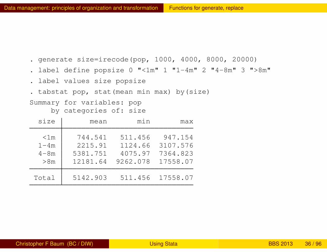
Stata contains both a recode command and a recode() function.These facilities may be used in lieu of a number of generate andreplace statements. There is also a irecode function to create anumeric code for values of a continuous variable falling in particularbrackets. For example, using a dataset containing population andmedian age for a number of US states:



. generate size=irecode(pop, 1000, 4000, 8000, 20000)

. label define popsize 0 "<1m" 1 "1-4m" 2 "4-8m" 3 ">8m"

. label values size popsize

. tabstat pop, stat(mean min max) by(size)

Summary for variables: popby categories of: size

size mean min max

<1m 744.541 511.456 947.1541-4m 2215.91 1124.66 3107.5764-8m 5381.751 4075.97 7364.823>8m 12181.64 9262.078 17558.07

Total 5142.903 511.456 17558.07



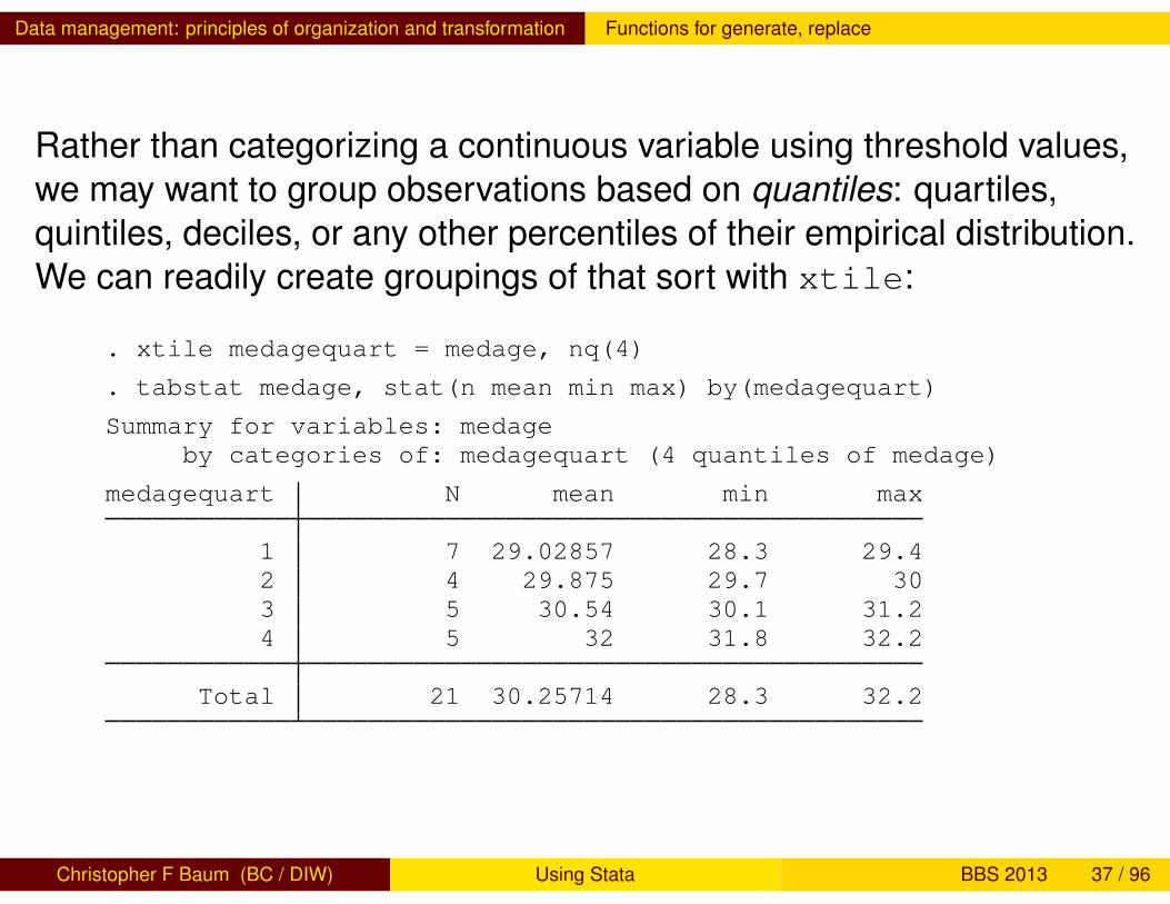
Rather than categorizing a continuous variable using threshold values,we may want to group observations based on quantiles: quartiles,quintiles, deciles, or any other percentiles of their empirical distribution.We can readily create groupings of that sort with xtile:

. xtile medagequart = medage, nq(4)

. tabstat medage, stat(n mean min max) by(medagequart)

Summary for variables: medageby categories of: medagequart (4 quantiles of medage)

medagequart N mean min max

1 7 29.02857 28.3 29.42 4 29.875 29.7 303 5 30.54 30.1 31.24 5 32 31.8 32.2

Total 21 30.25714 28.3 32.2


Data management: principles of organization and transformation String-to-numeric conversion and vice versa

String-to-numeric conversion

A problem that commonly arises with data transferred fromspreadsheets is the automatic classification of a variable as stringrather than numeric. This often happens if the first value of such avariable is NA, denoting a missing value. If Stata’s convention fornumeric missings—the dot, or full stop (.) is used, this will not occur. Ifone or more variables are misclassified as string, how can they bemodified?

First, a warning. Do not try to maintain long numeric codes (such asUS Social Security numbers, with nine digits) in numeric form, as theywill generally be rounded off. Treat them as string variables, which maycontain up to 244 bytes.



If a variable has merely been misclassified as string, the brute-forceapproach can be used:

generate patid = real( patientid )

Any values of patientid that cannot be interpreted as numeric willbe missing in patid. Note that this will also occur if numbers arestored with commas separating thousands.



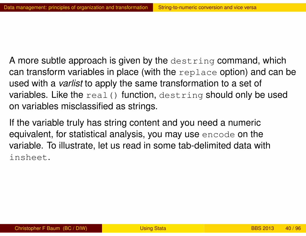
A more subtle approach is given by the destring command, whichcan transform variables in place (with the replace option) and can beused with a varlist to apply the same transformation to a set ofvariables. Like the real() function, destring should only be usedon variables misclassified as strings.

If the variable truly has string content and you need a numericequivalent, for statistical analysis, you may use encode on thevariable. To illustrate, let us read in some tab-delimited data withinsheet.



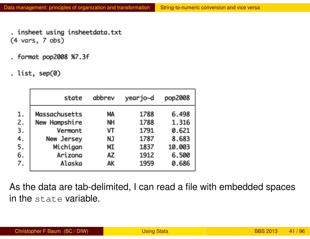
As the data are tab-delimited, I can read a file with embedded spacesin the state variable.



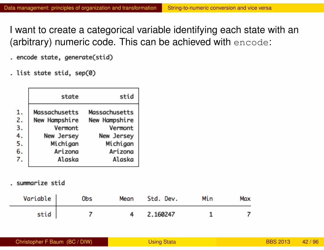
I want to create a categorical variable identifying each state with an(arbitrary) numeric code. This can be achieved with encode:



Although stid is a numeric variable (as summarize shows) it isautomatically assigned a value label consisting of the contents ofstate. The variable stid may now be used in analyses requiringnumeric variables.

You may also want to make a variable into a string (for instance, toreinstate leading zeros in an id code variable). You may use thestring() function, the tostring command or the decodecommand to perform this operation.


Data management: principles of organization and transformation The egen command

The egen command

Stata is not limited to using the set of defined generate functions.The egen (extended generate) command makes use of functionswritten in the Stata ado-file language, so that _gzap.ado would definethe extended generate function zap(). This would then be invoked as

egen newvar = zap(oldvar)

which would do whatever zap does on the contents of oldvar,creating the new variable newvar.

A number of egen functions provide row-wise operations similar tothose available in a spreadsheet: row sum, row average, row standarddeviation, and so on. Users may write their own egen functions. Inparticular, findit egenmore for a very useful collection.



Although the syntax of an egen statement is very similar to that ofgenerate, several differences should be noted. As only a subset ofegen functions allow a by varlist: prefix or by(varlist) option, thedocumentation should be consulted to determine whether a particularfunction is byable, in Stata parlance. Similarly, the explicit use of _nand _N, often useful in generate and replace commands is notcompatible with egen.



Wildcards may be used in row-wise functions. If you have state-levelU.S. Census variables pop1890, pop1900, ..., pop2000 youmay use egen nrCensus = rowmean(pop*) to compute theaverage population of each state over those decennial censuses. Therow-wise functions operate in the presence of missing values. Themean will be computed for all 50 states, although several were not partof the US in 1890.



The number of non-missing elements in the row-wise varlist may becomputed with rownonmiss(), with rowmiss() as thecomplementary value. Other official row-wise functions includerowmax(), rowmin(), rowtotal() and rowsd() (row standarddeviation). The functions rowfirst()and rowlast() give the first(last) non-missing values in the varlist. You may find this useful if thevariables refer to sequential items: for instance, wages earned peryear over several years, with missing values when unemployed.rowfirst() would return the earliest wage observation, androwlast() the most recent.



Official egen also provides a number of statistical functions whichcompute a statistic for specified observations of a variable and placethat constant value in each observation of the new variable. Sincethese functions generally allow the use of by varlist:, they may beused to compute statistics for each by-group of the data. This facilitatescomputing statistics for each household for individual-level data oreach industry for firm-level data. The count(), mean(), min(),max() and total() functions are especially useful in this context.

As an illustration using our state-level data, we egen the averagepopulation in each of the size groups defined above, and expresseach state’s population as a percentage of the average population inthat size group. Size category 0 includes the smallest states in oursample.



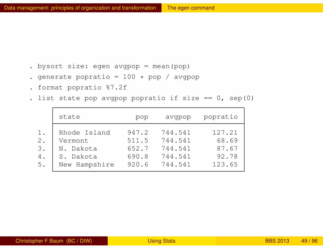
. bysort size: egen avgpop = mean(pop)

. generate popratio = 100 * pop / avgpop

. format popratio %7.2f

. list state pop avgpop popratio if size == 0, sep(0)

state pop avgpop popratio

1. Rhode Island 947.2 744.541 127.212. Vermont 511.5 744.541 68.693. N. Dakota 652.7 744.541 87.674. S. Dakota 690.8 744.541 92.785. New Hampshire 920.6 744.541 123.65



Other egen functions in this statistical category include iqr()(inter-quartile range), kurt() (kurtosis), mad() (median absolutedeviation), mdev() (mean absolute deviation), median(), mode(),pc() (percent or proportion of total), pctile(), p(n) (nth

percentile), rank(), sd() (standard deviation), skew() (skewness)and std() (z-score).

Many other egen functions are available; see help egen for details.


Data management: principles of organization and transformation Time series calendar

Time series calendar

Stata supports date (and time) variables and the creation of a timeseries calendar variable. Dates are expressed, as they are in Excel, asthe number of days from a base date. In Stata’s case, that date is1 Jan 1960 (like Unix/Linux). You may set up data on an annual,half-yearly, quarterly, monthly, weekly or daily calendar, as well as acalendar that merely uses the observation number.

You may also set the delta of the calendar variable to be other than1: for instance, if you have data at five-year intervals, you may definethe data as annual with delta=5. This ensures that the lagged valueof the 2005 observation is that of 2000.



An observation-number calendar is generally necessary forbusiness-daily data where you want to avoid gaps for weekends,holidays etc. which will cause lagged values and differences to containmissing values. However, you may want to create two calendarvariables for the same time series data: one for statistical purposesand one for graphical purposes, which will allow the series to begraphed with calendar-date labels. This procedure is illustrated in“Stata Tip 40: Taking care of business...”, Baum, CF. Stata Journal,2007, 7:1, 137-139.



A useful utility for setting the appropriate time series calendar istsmktim, available from the SSC Archive (ssc describetsmktim) and described in “Utility for time series data”, Baum, CF andWiggins, VL. Stata Technical Bulletin, 2000, 57, 2-4. It will set thecalendar, issuing the appropriate tsset command and the displayformat of the resulting calendar variable, and can be used in a paneldata context where each time series starts in the same calendarperiod.


Data management: principles of organization and transformation Time series operators

Time series operators

The D., L., and F. operators may be used under a time seriescalendar (including in the context of panel data) to specify firstdifferences, lags, and leads, respectively. These operators understandmissing data, and numlists: e.g. L(1/4).x is the first through fourthlags of x, while L2D.x is the second lag of the first difference of the xvariable.

It is important to use the time series operators to refer to lagged or ledvalues, rather than referring to the observation number (e.g., _n-1).The time series operators respect the time series calendar, and will notmistakenly compute a lag or difference from a prior period if it ismissing. This is particularly important when working with panel data toensure that references to one individual do not reach back into theprior individual’s data.


Data management: principles of organization and transformation Time series operators

Using time series operators, you may not only consistently generatedifferences, lags, and leads, but may refer to them ‘on the fly’ instatistical and estimation commands. That is, to estimate an AR(4)model, you need not create the lagged variables:

regress y L(1/4).y

or, to test Granger causality,

regress y L(-4/4).x

which would regress yt on four leads, four lags and the current value ofxt .

For a “Dickey–Fuller” style regression,

regress D.y L.y


Data management: principles of organization and transformation Factor variables

Factor variables

A valuable new feature in Stata version 11 and 12 is the factor variable.Stata has only one kind of numeric variable (although it supportsseveral different data types, which define the amount of storageneeded and possible range of values). However, if a variable iscategorical, taking on non-negative integer values, it may be used as afactor variable with the i. prefix.

The use of factor variables not only avoids explicit generation ofindicator (dummy) variables for each level of the categorical variable,but it means that the needed indicator variables are generated ‘on thefly’, as needed. Thus, to include the variable region, a categoricalvariable in census.dta which takes on values 1–4, we need onlyrefer to i.region in an estimation command.



This in itself merely mimics a preexisting feature of Stata: the xi:prefix. But factor variables are much more powerful, in that they can beused to define interactions, both with other factor variables and withcontinuous variables. Traditionally, you would define interactions bycreating new variables representing the product of two indicators, orthe product of an indicator with a continuous variable.

There is a great advantage in using factor variables rather thancreating new interaction variables. if you define interactions with thefactor variable syntax, Stata can then interpret the expression inpostestimation commands such as margins. For instance, you cansay i.race#i.sex, or i.sex#c.bmi, or c.bmi#c.bmi, where c.denotes a continuous variable, and # specifies an interaction.



With interactions between indicator and continuous variables specifiedin this syntax, we can evaluate the total effect of a change withoutfurther programming. For instance,

regress healthscore i.sex#c.bmi c.bmi#c.bmimargins, dydx(bmi) at(sex = (0 1))

which will perform the calculation of ∂healthscore/∂bmi for each levelof categorical variable sex, taking into account the squared term inbmi. We will discuss margins more fully in later talks in this series.


Combining data sets append

Combining data sets

In many empirical research projects, the raw data to be utilized arestored in a number of separate files: separate “waves” of panel data,timeseries data extracted from different databases, and the like. Stataonly permits a single data set to be accessed at one time. How, then,do you work with multiple data sets? Several commands are available,including append, merge, and joinby.

How, then, do you combine datasets in Stata? First of all, it isimportant to understand that at least one of the datasets to becombined must already have been saved in Stata format. Second, youshould realize that each of Stata’s commands for combining datasetsprovides a certain functionality, which should not confused with that ofother commands.



The append command

The append command combines two Stata-format data sets thatpossess variables in common, adding observations to the existingvariables. The same variables need not be present in both files, aslong as a subset of the variables are common to the “master” and“using” data sets. It is important to note that “PRICE" and “price” aredifferent variables, and one will not be appended to the other.



You might have a dataset on the demographic characteristics in 2007of the largest municipalities in China, cityCN. If you were given asecond dataset containing the same variables for the largestmunicipalities in Japan in 2007, cityJP, you might want to combinethose datasets with append. With the cityCN dataset in memory, youwould append using cityJP, which would add those records asadditional observations. You could then save the combined file under adifferent name. append can be used to combine multiple datasets, soif you had the additional files cityPH and cityMY, you could list thosefilenames in the using clause as well.

Prior to using append, it is a good idea to create an identifier variablein each dataset that takes on a constant value: e.g., gen country =1 in the CN dataset, gen country = 2 in the JP dataset, etc.



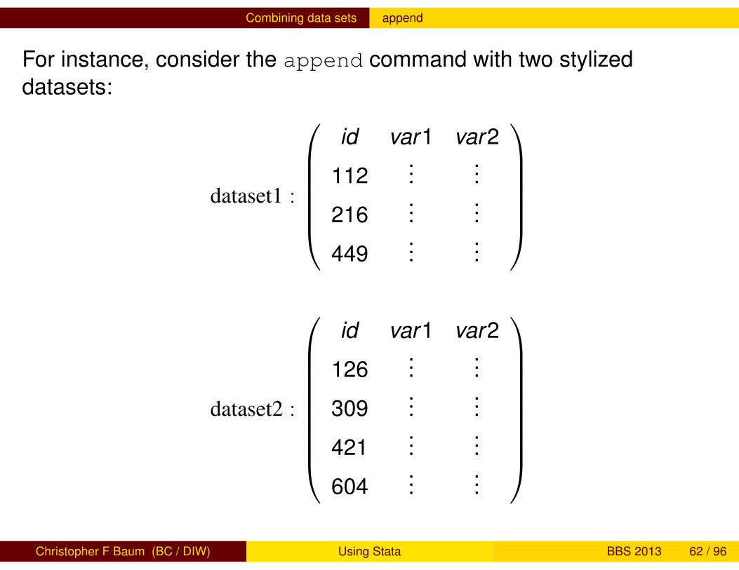
For instance, consider the append command with two stylizeddatasets:

dataset1 :

id var1 var2

112...

...

216...

...

449...

...

dataset2 :

id var1 var2

126...

...

309...

...

421...

...

604...

...



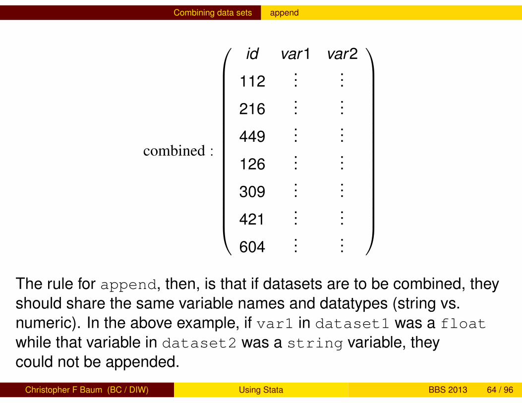
These two datasets contain the same variables, as they must forappend to sensibly combine them. If dataset2 contained idcode,Var1, Var2 the two datasets could not sensibly be appended withoutrenaming the variables (recall that in Stata, var1 and Var1 are twoseparate variables). Appending these two datasets with commonvariable names creates a single dataset containing all of theobservations:



combined :

id var1 var2

112...

...

216...

...

449...

...

126...

...

309...

...

421...

...

604...

...

The rule for append, then, is that if datasets are to be combined, theyshould share the same variable names and datatypes (string vs.numeric). In the above example, if var1 in dataset1 was a floatwhile that variable in dataset2 was a string variable, theycould not be appended.



It is permissible to append two datasets with differing variable names inthe sense that dataset2 could also contain an additional variable orvariables (for example, var3, var4). The values of those variables inthe observations coming from dataset1 would then be set to missing.

Some care must be taken when appending datasets in which the samevariable may exist with different data types (string in one, numeric inanother). For details, see “Stata tip 73: append with care!”, Baum CF,Stata Journal, 2008, 9:1, 166-168, included in your materials.


Combining data sets merge

The merge command

We now describe the merge command, which is Stata’s basic tool forworking with more than one dataset. Its syntax changed considerablyin Stata version 11.

The merge command takes a first argument indicating whether you areperforming a one-to-one, many-to-one, one-to-many or many-to-manymerge using specified key variables. It can also perform a one-to-onemerge by observation.



Like the append command, the merge works on a “master”dataset—the current contents of memory—and a single “using”dataset (prior to Stata 11, you could specify multiple using datasets).One or more key variables are specified, and in Stata 11 or 12 youneed not sort either dataset prior to merging.

The distinction between “master” and “using” is important. When thesame variable is present in each of the files, Stata’s default behavior isto hold the master data inviolate and discard the using dataset’s copyof that variable. This may be modified by the update option, whichspecifies that non-missing values in the using dataset should replacemissing values in the master, and the even stronger updatereplace, which specifies that non-missing values in the using datasetshould take precedence.



A “one-to-one” merge (written merge 1:1) specifies that each recordin the using data set is to be combined with one record in the masterdata set. This would be appropriate if you acquired additional variablesfor the same observations.

In any use of merge, a new variable, _merge, takes on integer valuesindicating whether an observation appears in the master only, theusing only, or appears in both. This may be used to determine whetherthe merge has been successful, or to remove those observationswhich remain unmatched (e.g. merging a set of households fromdifferent cities with a comprehensive list of postal codes; one wouldthen discard all the unused postal code records). The _merge variablemust be dropped before another merge is performed on this data set.



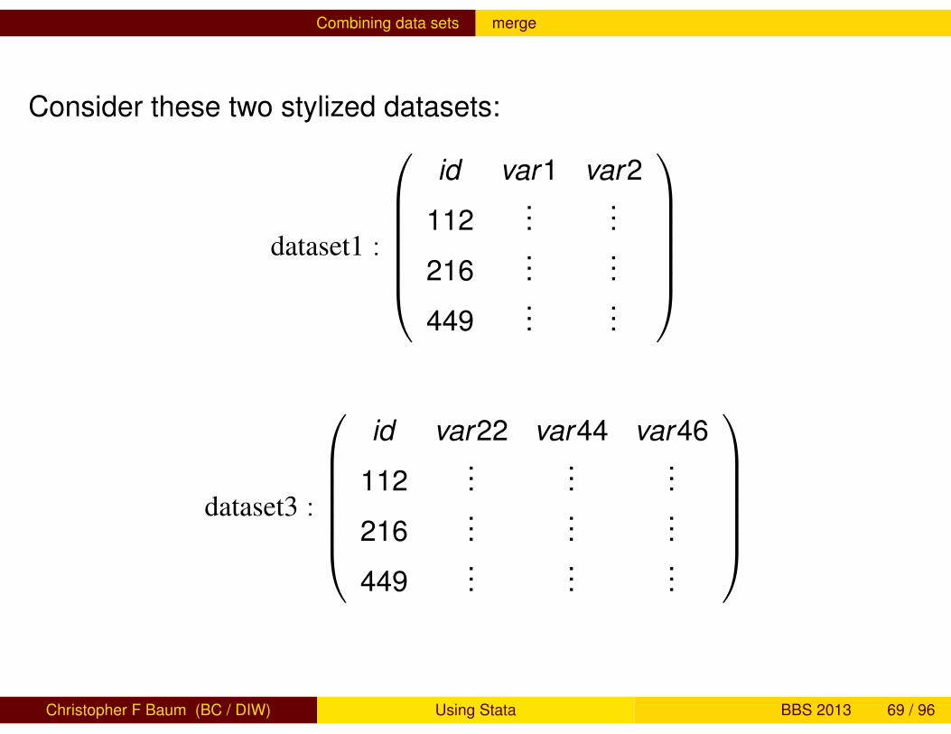
Consider these two stylized datasets:

dataset1 :

id var1 var2

112...

...

216...

...

449...

...

dataset3 :

id var22 var44 var46

112...

......

216...

......

449...

......



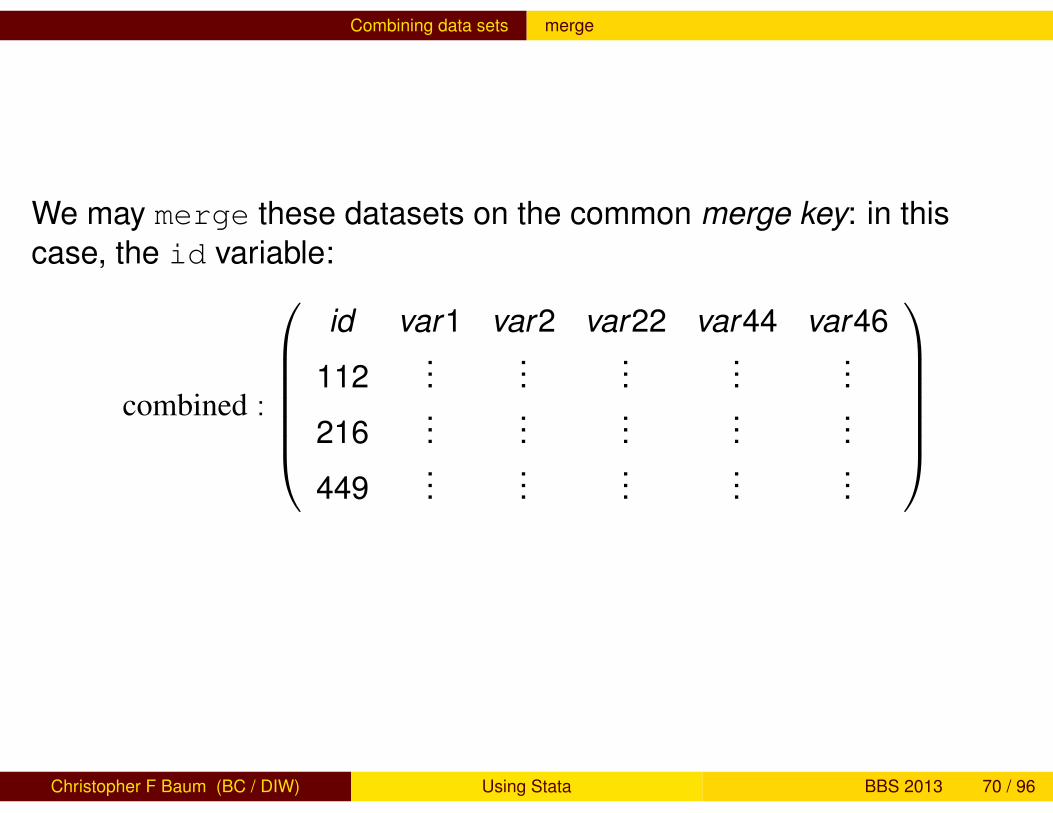
We may merge these datasets on the common merge key: in thiscase, the id variable:

combined :

id var1 var2 var22 var44 var46

112...

......

......

216...

......

......

449...

......

......



The rule for merge, then, is that if datasets are to be combined on oneor more merge keys, they each must have one or more variables with acommon name and datatype (string vs. numeric). In the exampleabove, each dataset must have a variable named id. That variable canbe numeric or string, but that characteristic of the merge key variablesmust match across the datasets to be merged. Of course, we need nothave exactly the same observations in each dataset: if dataset3contained observations with additional id values, those observationswould be merged with missing values for var1 and var2.

This is the simplest kind of merge: the one-to-one merge. Statasupports several other types of merges. But the key concept should beclear: the merge command combines datasets “horizontally”, addingvariables’ values to existing observations.


Combining data sets Match merge

The merge command can also do a “many-to-one"’ or “one-to-many”merge. For instance, you might have a dataset named hospitalsand a dataset named discharges, both of which contain a hospitalID variable hospid. If you had the hospitals dataset in memory,you could merge 1:m hospid using discharges to match eachhospital with its prior patients. If you had the discharges dataset inmemory, you could merge m:1 hospid using hospitals to addthe hospital characteristics to each discharge record. This is a veryuseful technique to combine aggregate data with disaggregate datawithout dealing with the details.

Although “many-to-one"’ or “one-to-many” merges are commonplaceand very useful, you should rarely want to do a “many-to-many” (m:m)merge, which will yield seemingly random results.


Combining data sets Match merge

The long-form dataset is very useful if you want to add aggregate-levelinformation to individual records. For instance, we may have paneldata for a number of companies for several years. We may want toattach various macro indicators (interest rate, GDP growth rate, etc.)that vary by year but not by company. We would place those macrovariables into a dataset, indexed by year, and sort it by year.

We could then use the firm-level panel dataset and sort it by year. Amerge command can then add the appropriate macro variables toeach instance of year. This use of merge is known as a one-to-manymatch merge, where the year variable is the merge key.

Note that the merge key may contain several variables: we might haveinformation specific to industry and year that should be merged ontoeach firm’s observations.


Reconfiguring data sets

Reconfiguring data sets

Data are often provided in a different orientation than that required forstatistical analysis. The most common example of this occurs withpanel, or longitudinal, data, in which each observation conceptuallyhas both cross-section (i) and time-series (t) subscripts. Often one willwant to work with a “pure” cross-section or “pure” time-series. If themicrodata themselves are the objects of analysis, this can be handledwith sorting and a loop structure. If you have data for N firms for Tperiods per firm, and want to fit the same model to each firm, onecould use the statsby command, or if more complex processing ofeach model’s results was required, a foreach block could be used. Ifanalysis of a cross-section was desired, a bysort would do the job.


Reconfiguring data sets collapse

But what if you want to use average values for each time period,averaged over firms? The resulting dataset of T observations can beeasily created by the collapse command, which permits you togenerate a new data set comprised of summary statistics of specifiedvariables. More than one summary statistic can be generated per inputvariable, so that both the number of firms per period and the averagereturn on assets could be generated. collapse can produce counts,means, medians, percentiles, extrema, and standard deviations.


Reconfiguring data sets reshape

Different models applied to longitudinal data require differentorientations of those data. For instance, seemingly unrelatedregressions (sureg) require the data to have T observations (“wide”),with separate variables for each cross–sectional unit. Fixed–effects orrandom-effects regression models xtreg, on the other hand, requirethat the data be stacked or “vec”’d in the “long” format. It is usuallymuch easier to generate transformations of the data in stacked format,where a single variable is involved.

The reshape command allows you to transfer the data from theformer (“wide”) format to the latter (“long”) format or vice versa. It is acomplicated command, because of the many variations on thisprocess one might encounter, but it is very powerful.



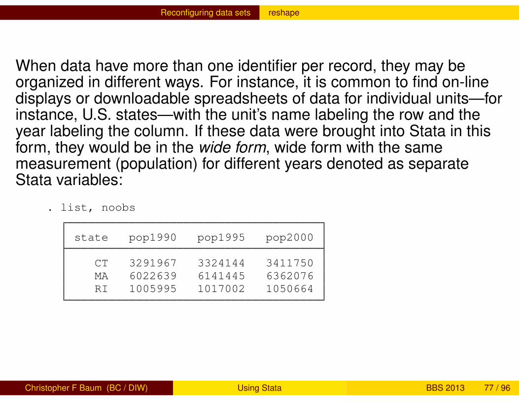
When data have more than one identifier per record, they may beorganized in different ways. For instance, it is common to find on-linedisplays or downloadable spreadsheets of data for individual units—forinstance, U.S. states—with the unit’s name labeling the row and theyear labeling the column. If these data were brought into Stata in thisform, they would be in the wide form, wide form with the samemeasurement (population) for different years denoted as separateStata variables:

. list, noobs

state pop1990 pop1995 pop2000

CT 3291967 3324144 3411750MA 6022639 6141445 6362076RI 1005995 1017002 1050664



There are a number of Stata commands—such as egen row-wisefunctions—which work effectively on data stored in the wide form. Itmay also be a useful form of data organization for producing graphs.

Alternatively, we can imagine stacking each year’s population figuresfrom this display into one variable, pop. In this format, known in Stataas the long form, each datum is identified by two variables: the statename and the year to which it pertains.



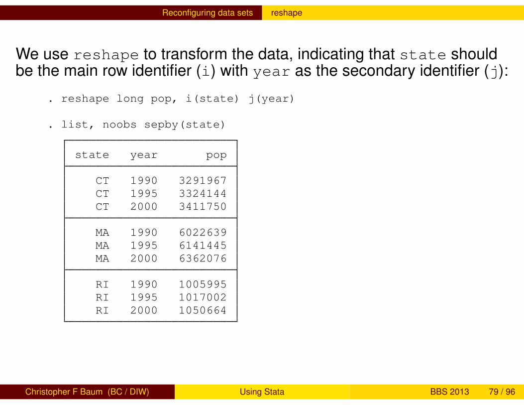
We use reshape to transform the data, indicating that state shouldbe the main row identifier (i) with year as the secondary identifier (j):

. reshape long pop, i(state) j(year)

. list, noobs sepby(state)

state year pop

CT 1990 3291967CT 1995 3324144CT 2000 3411750

MA 1990 6022639MA 1995 6141445MA 2000 6362076

RI 1990 1005995RI 1995 1017002RI 2000 1050664



This data structure is required for many of Stata’s statisticalcommands, such as the xt suite of panel data commands. The longform is also very useful for data management using by-groups and thecomputation of statistics at the individual level, often implemented withthe collapse command.

Inevitably, you will acquire data (either raw data or Stata datasets) thatare stored in either the wide or the long form and will find thattranslation to the other format is necessary to carry out your analysis.In statistical packages lacking a data-reshape feature, commonpractice entails writing the data to one or more external text files andreading it back in.



With the proper use of reshape, writing data out and reading themback in is not necessary in Stata. But reshape requires, first of all,that the data to be reshaped are labelled in such a way that they canbe handled by the mechanical rules that the command applies. Insituations beyond the simple application of reshape, it may requiresome experimentation to construct the appropriate command syntax.This is all the more reason for enshrining that code in a do-file as someday you are likely to come upon a similar application for reshape.

An illustration of advanced use of reshape on data from InternationalFinancial Statistics is provided in Baum CF, Cox NJ, “Stata tip 45:Getting those data into shape,” Stata Journal, 2007, 7, 268–271.


Producing publication-quality output and graphics Storing and retrieving estimates

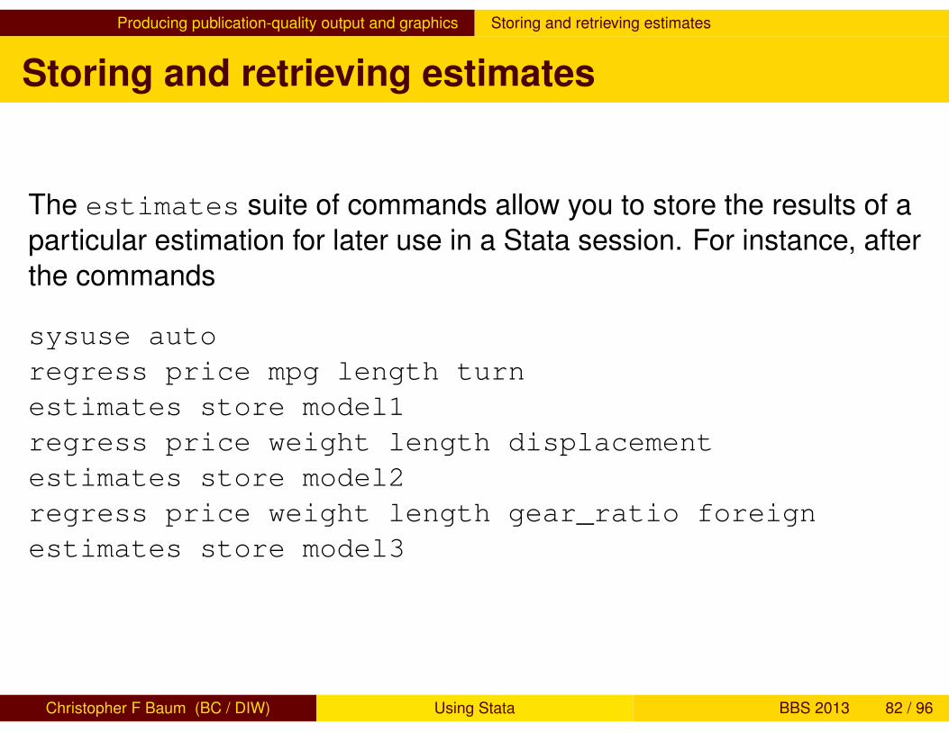
Storing and retrieving estimates

The estimates suite of commands allow you to store the results of aparticular estimation for later use in a Stata session. For instance, afterthe commands

sysuse autoregress price mpg length turnestimates store model1regress price weight length displacementestimates store model2regress price weight length gear_ratio foreignestimates store model3



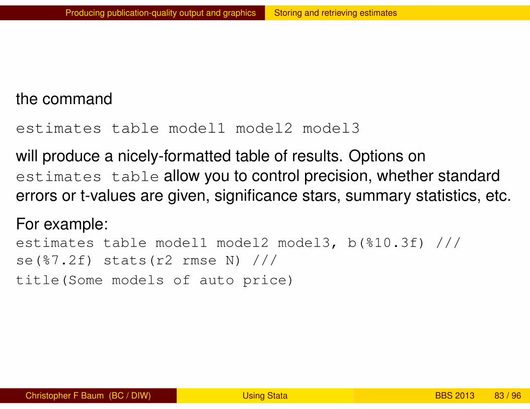
the command

estimates table model1 model2 model3

will produce a nicely-formatted table of results. Options onestimates table allow you to control precision, whether standarderrors or t-values are given, significance stars, summary statistics, etc.

For example:estimates table model1 model2 model3, b(%10.3f) ///se(%7.2f) stats(r2 rmse N) ///

title(Some models of auto price)



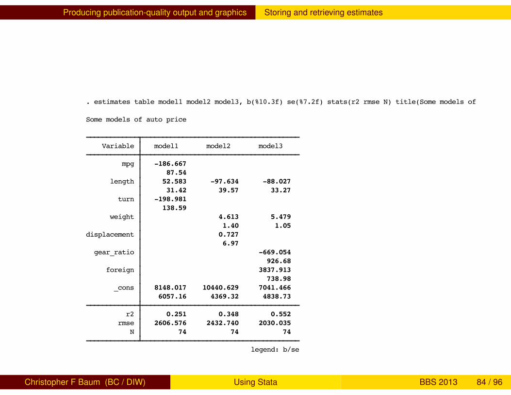
. estimates table model1 model2 model3, b(%10.3f) se(%7.2f) stats(r2 rmse N) title(Some models of auto price)

Some models of auto price

Variable model1 model2 model3

mpg -186.667 87.54 length 52.583 -97.634 -88.027 31.42 39.57 33.27 turn -198.981 138.59 weight 4.613 5.479 1.40 1.05 displacement 0.727 6.97 gear_ratio -669.054 926.68 foreign 3837.913 738.98 _cons 8148.017 10440.629 7041.466 6057.16 4369.32 4838.73

r2 0.251 0.348 0.552 rmse 2606.576 2432.740 2030.035 N 74 74 74

legend: b/se


Producing publication-quality output and graphics Publication-quality tables

Publication-quality tables

Although estimates table can produce a summary table quiteuseful for evaluating a number of specifications, we often want toproduce a publication-quality table for inclusion in a word processingdocument. Ben Jann’s estout command suite processes storedestimates and provides a great deal of flexibility in generating such atable.

Programs in the estout suite can produce tab-delimited tables for MSWord, HTML tables for the web, and—my favorite—LATEX tables forprofessional papers. In the LATEX output format, estout can generateGreek letters, sub- and superscripts, and the like. estout is availablefrom SSC, with extensive on-line help, and was described in the StataJournal, 5(3), 2005 and 7(2), 2007. It has its own website athttp://repec.org/bocode/e/estout.



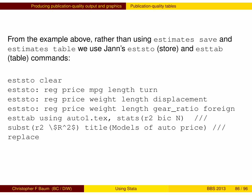
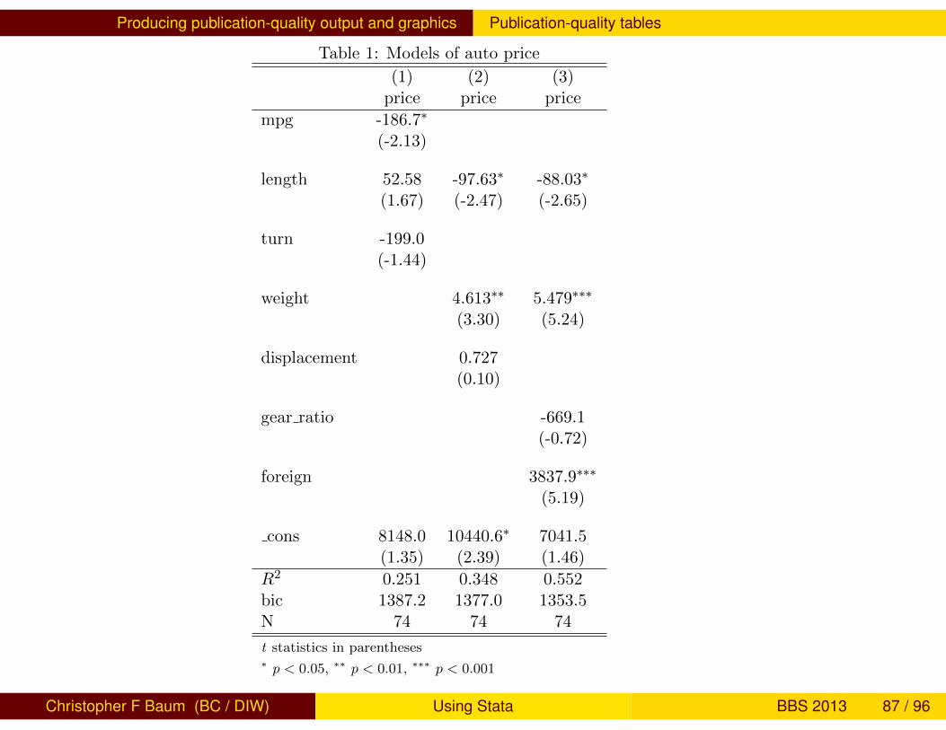
From the example above, rather than using estimates save andestimates table we use Jann’s eststo (store) and esttab(table) commands:

eststo cleareststo: reg price mpg length turneststo: reg price weight length displacementeststo: reg price weight length gear_ratio foreignesttab using auto1.tex, stats(r2 bic N) ///subst(r2 \$R^2$) title(Models of auto price) ///replace



Table 1: Models of auto price

(1) (2) (3)price price price

mpg -186.7∗

(-2.13)

length 52.58 -97.63∗ -88.03∗

(1.67) (-2.47) (-2.65)

turn -199.0(-1.44)

weight 4.613∗∗ 5.479∗∗∗

(3.30) (5.24)

displacement 0.727(0.10)

gear ratio -669.1(-0.72)

foreign 3837.9∗∗∗

(5.19)

cons 8148.0 10440.6∗ 7041.5(1.35) (2.39) (1.46)

R2 0.251 0.348 0.552bic 1387.2 1377.0 1353.5N 74 74 74

t statistics in parentheses∗ p < 0.05, ∗∗ p < 0.01, ∗∗∗ p < 0.001

1


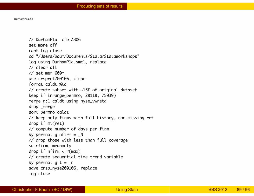
Producing sets of results


We illustrate how the computation of statistics on a per-firm basis canbe automated using daily CRSP stock returns data for 2001–2006. Inthis example, we create a subset of the full dataset, merge it with theNYSE value-weighted market return index, and restrict it to includeonly those firms with full coverage over the period.



Monday, March 7, 2011 3:25 AM Page 1

DurhamP1a.do

// DurhamP1a cfb A306set more offcapt log closecd "/Users/baum/Documents/Stata/StataWorkshops"log using DurhamP1a.smcl, replace// clear all// set mem 600muse crspret200106, clearformat caldt %td// create subset with ~15% of original datasetkeep if inrange(permno, 28118, 75039)merge n:1 caldt using nyse_vwretddrop _mergesort permno caldt// keep only firms with full history, non-missing retdrop if mi(ret)// compute number of days per firmby permno: g nfirm = _N// drop those with less than full coveragesu nfirm, meanonlydrop if nfirm < r(max)// create sequential time trend variableby permno: g t = _nsave crsp_nyse200106, replacelog close



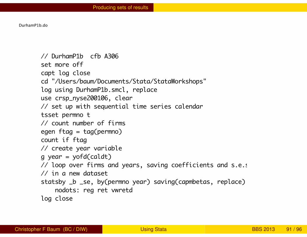
In the second step, we create a year variable from the daily calendar,and use the statsby prefix command to collect the coefficients andstandard errors from a CAPM regression of each firm’s return on themarket return, year by year, and save those results in a new Statadataset.



Monday, March 7, 2011 3:30 AM Page 1

DurhamP1b.do

// DurhamP1b cfb A306set more offcapt log closecd "/Users/baum/Documents/Stata/StataWorkshops"log using DurhamP1b.smcl, replaceuse crsp_nyse200106, clear// set up with sequential time series calendartsset permno t// count number of firmsegen ftag = tag(permno)count if ftag// create year variableg year = yofd(caldt)// loop over firms and years, saving coefficients and s.e.s// in a new datasetstatsby _b _se, by(permno year) saving(capmbetas, replace) ///

nodots: reg ret vwretdlog close



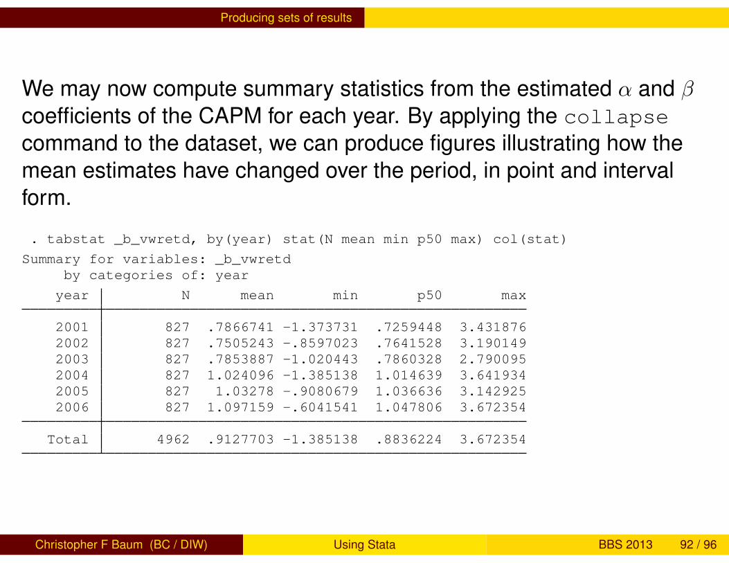
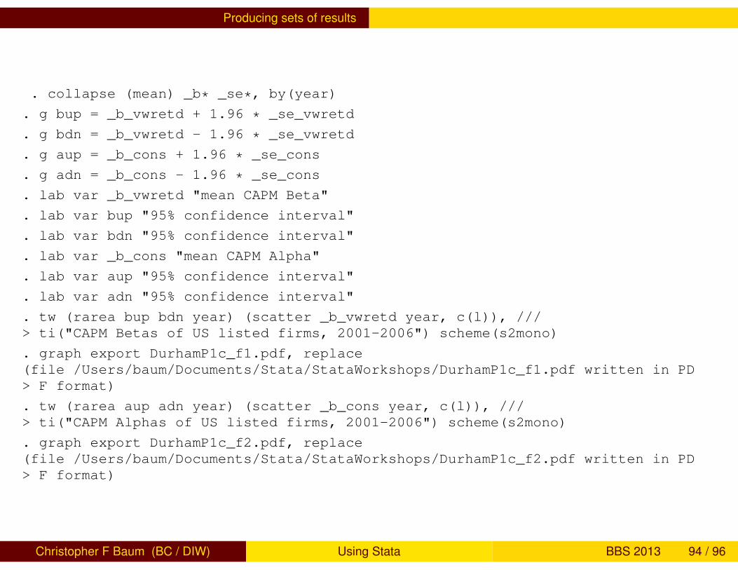
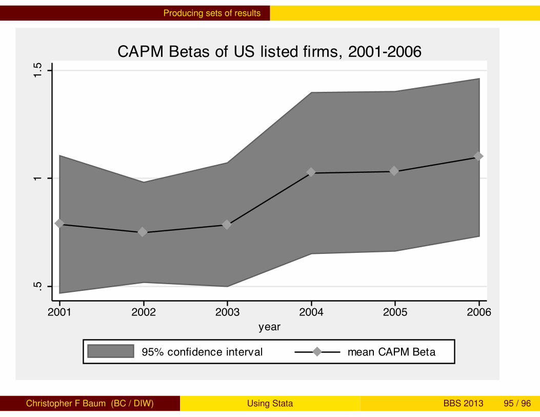
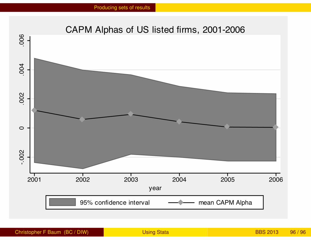
We may now compute summary statistics from the estimated α and βcoefficients of the CAPM for each year. By applying the collapsecommand to the dataset, we can produce figures illustrating how themean estimates have changed over the period, in point and intervalform.

. tabstat _b_vwretd, by(year) stat(N mean min p50 max) col(stat)

Summary for variables: _b_vwretdby categories of: year

year N mean min p50 max

2001 827 .7866741 -1.373731 .7259448 3.4318762002 827 .7505243 -.8597023 .7641528 3.1901492003 827 .7853887 -1.020443 .7860328 2.7900952004 827 1.024096 -1.385138 1.014639 3.6419342005 827 1.03278 -.9080679 1.036636 3.1429252006 827 1.097159 -.6041541 1.047806 3.672354

Total 4962 .9127703 -1.385138 .8836224 3.672354



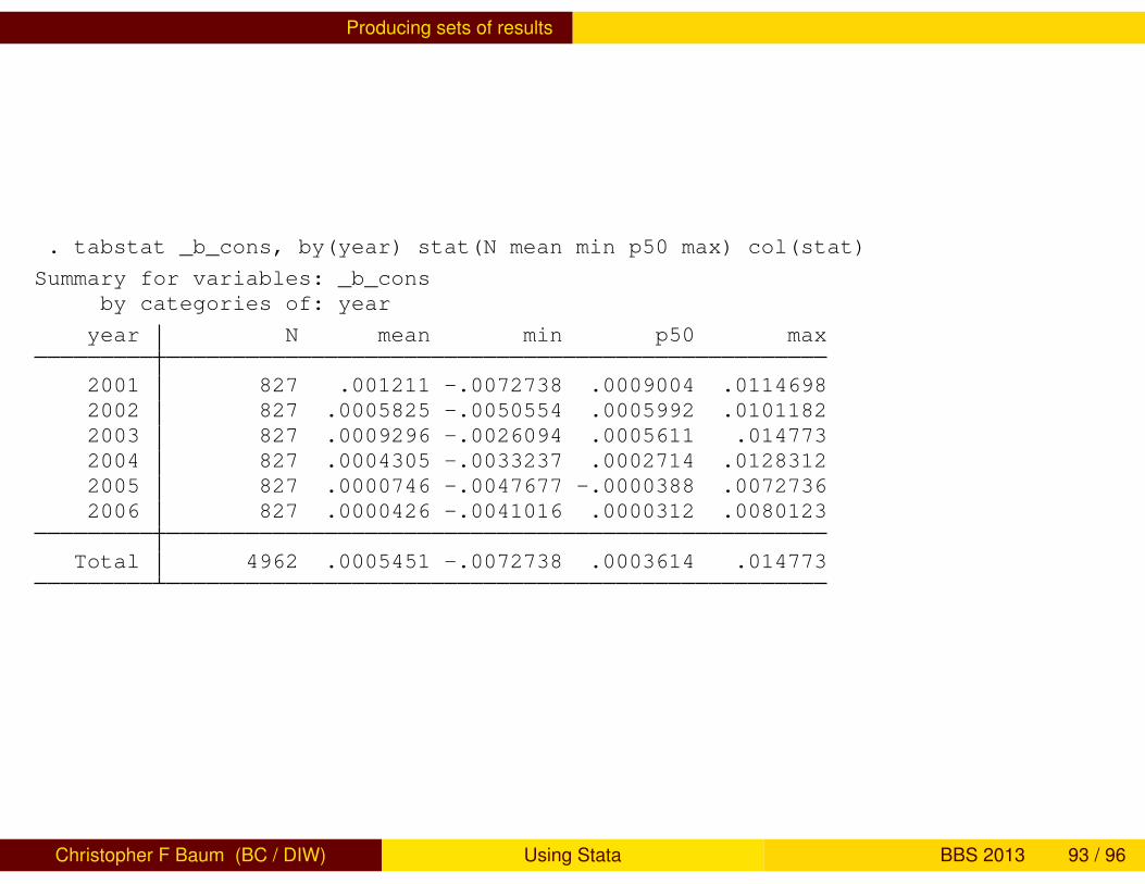
. tabstat _b_cons, by(year) stat(N mean min p50 max) col(stat)

Summary for variables: _b_consby categories of: year

year N mean min p50 max

2001 827 .001211 -.0072738 .0009004 .01146982002 827 .0005825 -.0050554 .0005992 .01011822003 827 .0009296 -.0026094 .0005611 .0147732004 827 .0004305 -.0033237 .0002714 .01283122005 827 .0000746 -.0047677 -.0000388 .00727362006 827 .0000426 -.0041016 .0000312 .0080123

Total 4962 .0005451 -.0072738 .0003614 .014773



. collapse (mean) _b* _se*, by(year)

. g bup = _b_vwretd + 1.96 * _se_vwretd

. g bdn = _b_vwretd - 1.96 * _se_vwretd

. g aup = _b_cons + 1.96 * _se_cons

. g adn = _b_cons - 1.96 * _se_cons

. lab var _b_vwretd "mean CAPM Beta"

. lab var bup "95% confidence interval"

. lab var bdn "95% confidence interval"

. lab var _b_cons "mean CAPM Alpha"

. lab var aup "95% confidence interval"

. lab var adn "95% confidence interval"

. tw (rarea bup bdn year) (scatter _b_vwretd year, c(l)), ///> ti("CAPM Betas of US listed firms, 2001-2006") scheme(s2mono)

. graph export DurhamP1c_f1.pdf, replace(file /Users/baum/Documents/Stata/StataWorkshops/DurhamP1c_f1.pdf written in PD> F format)

. tw (rarea aup adn year) (scatter _b_cons year, c(l)), ///> ti("CAPM Alphas of US listed firms, 2001-2006") scheme(s2mono)

. graph export DurhamP1c_f2.pdf, replace(file /Users/baum/Documents/Stata/StataWorkshops/DurhamP1c_f2.pdf written in PD> F format)



.51

1.5

2001 2002 2003 2004 2005 2006year

95% confidence interval mean CAPM Beta

CAPM Betas of US listed firms, 2001-2006



-.002

0.0

02.0

04.0

06

2001 2002 2003 2004 2005 2006year

95% confidence interval mean CAPM Alpha

CAPM Alphas of US listed firms, 2001-2006


Christopher F Baum - University of Birmingham · Using Stata for data management and reproducible...

Documents

Transcript of Christopher F Baum - University of Birmingham · Using Stata for data management and reproducible...