CHOMP: Gradient Optimization Techniques for Efficient Motion Planning

Nathan Ratliff1 Matt Zucker1 J. Andrew Bagnell1 Siddhartha Srinivasa2

1The Robotics Institute 2Intel ResearchCarnegie Mellon University Pittsburgh, PA

{ndr, mzucker, dbagnell}@cs.cmu.edu siddhartha.srinivasa@intel.com

Abstract— Existing high-dimensional motion planning algo-rithms are simultaneously overpowered and underpowered. Indomains sparsely populated by obstacles, the heuristics used bysampling-based planners to navigate “narrow passages” can beneedlessly complex; furthermore, additional post-processing isrequired to remove the jerky or extraneous motions from thepaths that such planners generate. In this paper, we presentCHOMP, a novel method for continuous path refinement thatuses covariant gradient techniques to improve the quality ofsampled trajectories. Our optimization technique convergesover a wider range of input paths and is able to optimize higher-order dynamics of trajectories than previous path optimizationstrategies. As a result, CHOMP can be used as a standalonemotion planner in many real-world planning queries. Theeffectiveness of our proposed method is demonstrated in ma-nipulation planning for a 6-DOF robotic arm as well as intrajectory generation for a walking quadruped robot.

I. INTRODUCTION

In recent years, sampling-based planning algorithms havemet with widespread success due to their ability to rapidlydiscover the connectivity of high-dimensional configura-tion spaces. Planners such as the Probabilistic Roadmap(PRM) and Rapidly-exploring Random Tree (RRT) algo-rithms, along with their descendents, are now used in amultitude of robotic applications [15], [16]. Both algorithmsare typically deployed as part of a two-phase process: firstfind a feasible path, and then optimize it to remove redundantor jerky motion.

Perhaps the most prevalent method of path optimizationis the so-called “shortcut” heuristic, which picks pairs ofconfigurations along the path and invokes a local planner toattempt to replace the intervening sub-path with a shorterone [14], [5]. “Partial shortcuts” as well as medial axisretraction have also proven effective [11]. Another approachused in elastic bands or elastic strips planning involvesmodeling paths as mass-spring systems: a path is assignedan internal energy related to its length or smoothness, alongwith an external energy generated by obstacles or task-based potentials. Gradient based methods are used to finda minimum-energy path [20], [4].

In this paper we present Covariant Hamiltonian Optimiza-tion and Motion Planning (CHOMP), a novel method forgenerating and optimizing trajectories for robotic systems.The approach shares much in common with elastic bandsplanning; however, unlike many previous path optimizationtechniques, we drop the requirement that the input path becollision free. As a result, CHOMP can often transform a

Fig. 1. Experimental robotic platforms: Boston Dynamic’s LittleDog (left),and Barrett Technologys’s WAM arm (right).

naıve initial guess into a trajectory suitable for execution ona robotic platform without invoking a separate motion plan-ner. A covariant gradient update rule ensures that CHOMPquickly converges to a locally optimal trajectory.

In many respects, CHOMP is related to optimal control ofrobotic systems. Instead of merely finding feasible paths, ourgoal is to directly construct trajectories which optimize overa variety of dynamic and task-based criteria. Few currentapproaches to optimal control are equipped to handle obsta-cle avoidance, though. Of those that do, many approachesrequire some description of configuration space obstacles,which can be prohibitive to create for high-dimensionalmanipulators [25]. Many optimal controllers which do handleobstacles are framed in terms of mixed integer programming,which is known to be an NP-hard problem [24], [9], [17],[27]. Approximate optimal algorithms exist, but so far, onlyconsider very simple obstacle representations [26].

In the rest of this document, we give a detailed derivationof the CHOMP algorithm, show experimental results ona 6-DOF robot arm, detail the application of CHOMP toquadruped robot locomotion, and outline future directions ofwork. The accompanying video in the conference proceed-ings also contains examples of running CHOMP on bothrobot platforms.

II. THE CHOMP ALGORITHM

In this section, we present CHOMP, a new trajectory opti-mization procedure based on covariant gradient descent. Animportant theme throughout this exposition is the proper useof geometrical relations, particularly as they apply to innerproducts. This is a particularly important idea in differentialgeometry [8]. These considerations appear in three primary

locations within our technique. First, we find that in orderto encourage smoothness we need measure the size of anupdate to our hypothesis in terms of the amount of dynamicalquantity (such as total velocity or total acceleration) it addsto the trajectory. Second, measurements of obstacle costsshould be taken in the workspace so as to correctly accountfor the geometrical relationship between the robot and thesurrounding environment. And finally, the same geometricalconsiderations used to update a trajectory should be usedwhen correcting any joint limit violations that may occur.Sections II-A, II-D, and II-F detail each of these points inturn.

A. Covariant Gradient Descent

Formally, our goal is to find a smooth, collision-free,trajectory through the configuration space Rm between twoprespecified end points qinit, qgoal ∈ Rm. In practice, wediscretize our trajectory into a set of n waypoints q1, . . . , qn

(excluding the end points) and compute dynamical quan-tities via finite differencing. We focus presently on finite-dimensional optimization, although we will return to thecontinuous trajectory setting in section II-D. Section II-E,discusses the relationship between these settings.

We model the cost of a trajectory using two terms: anobstacle term fobs, which measures the cost of being nearobstacles; and a prior term fprior, which measures dynamicalquantities of the robot such as smoothness and acceleration.We generally assume that fprior is independent of theenvironment. Our objective can, therefore, be written

U(ξ) = fprior(ξ) + fobs(ξ).

More precisely, the prior term is a sum of squared derivatives.Given suitable finite differencing matrices Kd for d =1, . . . , D, we can represent the function as a sum of terms

fprior(ξ) =12

D∑d=1

wd ‖Kd ξ + ed‖2 , (1)

where ed are constant vectors that encapsulate the contri-butions from the fixed end points. For instance, the firstterm (d = 1) represents the total squared velocity along thetrajectory. In this case, we can write K1 and e1 as

K1 =

1 0 0 . . . 0 0−1 1 0 . . . 0 00 −1 1 . . . 0 0

.... . .

...0 0 0 . . . −1 10 0 0 . . . 0 −1

⊗ Im×m

e1 =[−qT

0 , 0, . . . , 0, qTn+1

]T.

where ⊗ denotes the Kronecker (tensor) product. We notethat fprior is a simple quadratic form:

fprior(ξ) =12ξT A ξ + ξT b + c

for suitable matrix, vector, and scalar constants A, b, c. Wenote that A is symmetric positive definite for all d.

We seek to improve the trajectory by iteratively mini-mizing a local approximation of the function using onlysmooth updates, where we define smoothness as measuredby equation 1. At iteration k, within a region of our currenthypothesis ξk, we can approximate our objective using afirst-order Taylor expansion:

U(ξ) ≈ U(ξk) + gTk (ξ − ξk), (2)

where gk = ∇U(ξk). Our update can be written formally as

ξk+1 = arg minξ

{U(ξk) + gT

k (ξ − ξk) +λ

2‖ξ − ξk‖2M

},

(3)

where the notation ‖δ‖2M denotes the norm of the displace-ment δ = ξ−ξk taken with respect to the Riemannian metricM equal to δT M δ. Setting the gradient of the right handside of equation 3 to zero and solving results in the followingmore succinct rule:

ξk+1 = ξk −1λ

M−1gk

It is well known in optimization theory that solving a regu-larized problem of the form given in equation 3 is equivalentto minimizing the linear approximation in equation 2 withina ball around ξk whose radius is related to the regularizationconstant λ [3]. Since under the metric A, the norm of non-smooth trajectories is large, this ball contains only smoothupdates δ = ξ − ξk, Our update rule, therefore, servesto ensure that the trajectory remains smooth after eachtrajectory modification.

B. Understanding the Update Rule

This update rule is a special case of a more general ruleknown as Covariant gradient descent [2], [29], in which thematrix A need not be constant.1 In our case, it is useful tointerpret the action of the inverse operator A−1 as spreadingthe gradient across the entire trajectory. As an example, wetake d = 1 and note that A is a finite differencing operator forapproximating accelerations. Since AA−1 = I , we see thatthe ith column/row of A−1 has zero acceleration everywhere,except at the ith entry. A−1gk can, therefore, be viewed asa vector of projections of gk onto the set of smooth basisvectors forming A−1.

CHOMP is covariant in the sense that the change to thetrajectory that results from the update is a function only ofthe trajectory itself, and not the particular representation used(e.g. waypoint based)– at least in the limit of small step sizeand fine discretization. This normative approach makes iteasy to derive the CHOMP update rule: we can understandequation 3 as the Langrangian form of an optimizationproblem [1] that attempts to maximize the decrease in ourobjective function subject to making only a small changein the average acceleration of the resulting trajectory– notsimply making a small change in the parameters that definethe trajectory in a particular representation.

1In the most general setting, the matrix A may vary smoothly as afunction of the domain ξ.

We gain additional insight into the computational benefitsof the covariant gradient based update by considering theanalysis tools developed in the online learning/optimizationliterature and especially [28], [12]. Analyzing the behavior ofthe CHOMP update rule in the general case is very difficultto characterize. However, by considering in a region arounda local optima sufficiently small that fobs is convex we cangain insight into the performance of both standard gradientmethods (including those considered by, e.g. [20]) and theCHOMP rule.

We first note that under these conditions, the overallCHOMP objective function is strongly convex [22]– that is,it can be lower-bounded over the entire region by a quadraticwith curvature A. [12] shows how gradient-style updates canbe understood as sequentially minimizing a local quadraticapproximation to the objective function. Gradient descentminimizes an uninformed, isotropic quadratic approximationwhile more sophisticated methods, like Newton steps, com-pute tighter lower bounds using a Hessian. In the case ofCHOMP, the Hessian need not exist as our objective functionmay not even be differentiable, however we may still form aquadratic lower bound using A. This is much tighter thanan isotropic bound and leads to a correspondingly fasterminimization of our objective– in particular, in accordancewith the intuition of adjusting large parts of the trajectory dueto the impact at a single point we would generally expect it tobe O(n) times faster to converge than a standard, Euclideangradient based method that adjusts a single point due anobstacle.

Importantly, we note that we are not simulating a mass-spring system as in [20]. We instead formulate the problem ascovariant optimization in which we optimize directly withinthe space of trajectories. In [19], a similar optimizationsetting is discussed, although, more traditional Euclideangradients are derived. We demonstrate below that optimizingwith respect to our smoothness norm substantially improvesconvergence.

In our experiments, we additionally implemented a versionof this algorithm based on Hamiltonian Monte Carlo [18],[29]. This variant is a Monte Carlo sampling techniquethat utilizes gradient information and energy conservationconcepts to efficiently navigate equiprobability curves ofan augmented state-space. It can essentially be viewed asa well formulated method of adding noise to the system;importantly, the algorithm is guaranteed to converge to astationary distribution inversely proportional to the exponen-tiated objective function.

Hamiltonian Monte Carlo provides a first step toward acomplete motion planner built atop these concepts. However,as we discuss in section V, while the algorithm solvesa substantially larger breadth of planning problems thantraditional trajectory optimization algorithms, it still fallsprey to local minima for some more difficult problems whenconstrained by practical time limitations.

0

0

εd(x)

c(x)

Fig. 2. Potential function for obstacle avoidance

C. Obstacles and Distance Fields

Let B denote the set of points comprising the robot body.When the robot is in configuration q, the workspace locationof the element u ∈ B is given by the function

x(q, u) : Rm × B 7→ R3

A trajectory for the robot is then collision-free if for everyconfiguration q along the trajectory and for all u ∈ B, thedistance from x(q, u) to the nearest obstacle is greater thanε ≥ 0.

If obstacles are static and the description of B is geometri-cally simple, it becomes advantageous to simply precomputea signed distance field d(x) which stores the distance from apoint x ∈ R3 to the boundary of the nearest obstacle. Valuesof d(x) are negative inside obstacles, positive outside, andzero at the boundary.

Computing d(x) on a uniform grid is straightforward.We start with a boolean-valued voxel representation of theenvironment, and compute the Euclidean Distance Transform(EDT) for both the voxel map and its logical complement.The signed distance field is then simply given by thedifference of the two EDT values. Computing the EDT issurprisingly efficient: for a lattice of K samples, computationtakes time O(K) [10].

When applying CHOMP, we typically use a simplifiedgeometric description of our robots, approximating the robotas a “skeleton” of spheres and capsules, or line-segmentswept spheres. For a sphere of radius r with center x, thedistance from any point in the sphere to the nearest obstacleis no less than d(x) − r. An analogous lower bound holdsfor capsules.

There are a few key advantages of using the signeddistance field to check for collisions. Collision checking isvery fast, taking time proportional to the number of voxelsoccupied by the robot’s “skeleton”. Since the signed distancefield is stored over the workspace, computing its gradient viafinite differencing is a trivial operation. Finally, because wehave distance information everywhere, not just outside ofobstacles, we can generate a valid gradient even when therobot is in collision – a particularly difficult feat for otherrepresentations and distance query methods.

Now we can define the workspace potential function c(x),which penalizes points of the robot for being near obstacles.The simplest such function might simply be

c(x) = max(ε− d(x), 0

)

A smoother version, shown in figure 2, is given by

c(x) =

−d(x) + 12 ε, if d(x) < 0

12 ε (d(x)− ε)2, if 0 ≤ d(x) ≤ ε

0, otherwise

D. Defining an obstacle potential

We will switch for a moment to discussing optimizationof a continuous trajectory q(t) by defining our obstaclepotential as a functional over q. As we show in the nextsection, we could also derive the objective over a prespecifieddiscretization, but we find that the properties of the objectivefunction more clearly present themselves in the functionalsetting.

To begin, we define a workspace potential c : R3 → R

that quantifies the cost of a body element u ∈ B of the robotresiding at a particular point x in the workspace.

Intuitively, we would like to integrate these cost valuesacross the entire robot. A straightforward integration acrosstime, however, is undesirable since moving more quicklythrough regions of high cost will be penalized less. Instead,we choose to integrate the cost elements with respect to anarc-length parameterization. Such an objective will have nomotivation to alter the velocity profile along the trajectorysince such operations do not change the trajectory’s length.We will see that this intuition manifests itself in the func-tional gradient as a projection of workspace gradients of c(x)onto the two-dimensional plane orthogonal to the directionof motion of a body element u through the workspace.

We therefore write our obstacle objective as

fobs[q] =∫ 1

0

∫u

c

(x(q(t), u

)) ∥∥∥∥ d

dtx(q(t), u

)∥∥∥∥ du dt

Since fobs depends only on workspace positions and veloc-ities (and no higher order derivatives), we can derive thefunctional gradient as ∇fobs = ∂v

∂q −ddt

∂v∂q′ , where v denotes

everything inside the time integral [7], [19]. Applying thisformula to fobs, we get

∇fobs =∫

u

JT[‖x′‖

((I − x′x′T

)∇c− cκ

)]du (4)

where κ is the curvature vector [8] defined as

κ =1

‖x′‖2(I − x′x′T

)x′′

and J is the kinematic Jacobian ∂∂q x(q, u). To simplify the

notation we have suppressed the dependence of J , x, and con integration variables t and u. We additionally denote timederivatives of x(q(t), u) using the traditional prime notation,and we denote normalized vectors by x.

This objective function is similar to that discussed insection 3.12 of [19]. However, there is an important dif-ference that substantially improves performance in practice.Rather than integrating with respect to arc-length throughconfiguration space, we integrate with respect to arc-lengthin the workspace. This simple modification represents afundamental change: instead of using the Euclidean geometry

Fig. 3. Left: A simple two-dimensional trajectory traveling through anobstacle potential (with large potentials are in red and small potentials inblue). The gradient at each configuration of the discretization depicted as agreen arrow. Right: A plot of both the continuous functional gradient givenin red and the corresponding Euclidean gradient component values of thediscretization at each way point in blue.

in the configuration space, we directly utilize the geometryof the workspace.

Intuitively, we can more clearly see the distinction byexamining the functional gradients of the two formulations.Operationally, the functional gradient defined in [19] can becomputed in two steps. First, we integrate across all bodyelements the configuration space gradient contributions thatresult from transforming each body element’s workspacegradient through the corresponding Jacobian. Second, weproject that single summarizing vector orthogonally to thetrajectory’s direction of motion in the configuration space.Alternatively, our objective performs this projection directlyin the workspace before the transformation and integrationsteps. This ensures that orthogonality is measured withrespect to the geometry of the workspace.

In practice, to implement these updates on a discretetrajectory ξ we approximate time derivatives using finitedifferences wherever they appear in the objective and itsfunctional gradient. (The Jacobian J , of course, can becomputed using the straightforward Jacobian of the robot.)

E. Functions vs Functionals

Although section II-A presents our algorithm in termsof a specific discretization, writing the objective in termsof functionals over continuous trajectories often enunciatesits properties. Section II-D exemplifies this observation.As figure 3 demonstrates, the finite-dimensional Euclideangradient of a discretized version of the functional

fobs(ξ) =n∑

t=1

U∑u=1

12

(c(xu(qt+1)

)+ c

(xu(qt)

) )·∥∥xu(qt+1)− xu(qt)∥∥

converges rapidly to the functional gradient as the resolutionof the discretization increases. (In this expression, we denotethe forward kinematics mapping of configuration q to bodyelement i using xu(q).) However, the gradient of any finite-dimensional discretization of the fobs takes on a substantiallydifferent form; the projection properties that are clearlyidentified in the functional gradient (equation 4) are no longerobvious.

We note that the prior term can be written as a functionalas well:

fprior[ξ] =D∑

d=1

∫ 1

0

‖q′(t)‖2dt,

with functional gradient

∇fprior[ξ] =D∑

d=1

(−1)dq(2d)

In this case, a discretization of the functional gradient g =(∇fprior[ξ](ε), . . . , ∇fprior[ξ](ε)(1−ε))T exactly equals thegradient of the discretized prior when central differences areused to approximate the derivatives.

F. Smooth projection for joint limits and other issues

Joint limits are traditionally handled by either adding anew potential to the objective function which penalizes thetrajectory for approaching the limits, or by performing asimple projection back onto the set of feasible joint valueswhen a violation of the limits is detected. In our experiments,we follow the latter approach. However, rather than simplyresetting the violating joints back to their limit values, whichcan be thought of as a L1 projection on to the set of feasiblevalues, we implement an approximate projection techniquethat projects with respect to the norm defined by the matrixA defined in section II-A.

At each iteration, we first find the vector of updates v thatwould implement the L1 projection when added to the trajec-tory. However, before adding it, we transform that vector bythe inverse of our metric A−1. As discussed in section II-A,this transformation effectively smooths the vector across theentire trajectory so that the resulting update vector has smallacceleration. As a result, when we add a scaled version ofthat vector to our trajectory ξ, we can simultaneously removethe violations while retaining smoothness.

Our projection algorithm is listed formally below. Asindicated, we may need to iterate this procedure sincethe smoothing operation degrades a portion of the originalprojection signal. However, in our experiments, all joint limitviolations were corrected within a single iteration of thisprocedure. Figure 4 plots the final joint angle curves overtime from the final optimized trajectory on a robotic arm (seesection III). The fourth subplot typifies the behavior of thisprocedure. While L1 projection often produces trajectoriesthat threshold at the joint limit, projection with respect tothe acceleration norm produces a smooth joint angle tracewhich only briefly brushes the joint limit as a tangent.

Smooth projection:1) Compute the update vector v used for L1 projection.2) Transform the vector via our Riemannian metric v =

A−1v.3) Scale the resulting vector by α such that ξ = ξ + αv

entirely removes the largest joint limit violation.4) Iterate if violations remain.

III. EXPERIMENTS ON A ROBOTIC ARM

This section presents experimental results for our im-plementation of CHOMP on Barrett Technologies’s WAMarm shown in figure 1. We demonstrate the efficacy ofour technique on a set of tasks typically encountered in ahome manipulation setting. The arm has seven degrees offreedom, although, we planned using only the first six inthese experiments.2

A. Collision heuristic

The home setting differs from setting such as those en-countered in legged locomotion (see section IV) in that theobstacles are often thin (e.g. they may be pieces of furnituresuch as tables or doors). Section II-C discusses a heuristicbased on the signed distance field under which the obstaclesthemselves specify how the robot should best remove itselffrom collision. While this works well when the obstacle isa large body, such as the terrain as in the case of leggedlocomotion, this heuristic can fail for smaller obstacles. Aninitial straight-line trajectory through configuration spaceoften contains configurations that pass entirely through anobstacle. In that case, the naıve workspace potential workstends to simultaneously push the robot out of collision on oneside, but also, to pull the robot further through the obstacleon the other side.

We avoid this behavior by adding an indicator function tothe objective that makes all workspace terms that appear afterthe first collision along the arm (as ordered via distance to thebase) vanish. This indicator factor can be written mathemat-ically as I(minj≤i d(xj(q)), although implementationally itis implemented simply by ignoring all terms after the firstcollision while iterating from the base of the body out towardthe end effector for a given time step of the trajectory.

Intuitively, this heuristic suggests simply that theworkspace gradients encountered after then first collision ofa given configuration are invalid and should therefore beignored. Since we know the base of the robotic arm is alwayscollision free, we are assured of a region along the arm priorto the first collision that can work to pull the rest of the armout of collision. In our experiments, this heuristic works wellto pull the trajectory free of obstacles typically encounteredin the home environment.

B. Experimental results

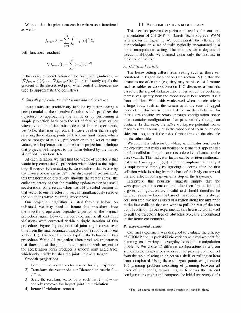
Our first experiment was designed to evaluate the efficacyof CHOMP and its probabilistic variants as a replacement forplanning on a variety of everyday household manipulationproblems. We chose 15 different configurations in a givenscene representing various tasks such as picking up an objectfrom the table, placing an object on a shelf, or pulling an itemfrom a cupboard. Using these start/goal points we generated105 planning problem consisting of planning between allpairs of end configurations. Figure 6 shows the 15 endconfigurations (right) and compares the initial trajectory (left)

2The last degree of freedom simply rotates the hand in place.

Fig. 4. Left: This figure shows the joint angle traces that result from running CHOMP on the robot arm described in section III using the smoothprojection procedure discussed in section II-F. Each subplot shows a different joint’s trace across the trajectory in blue with upper and lower joint limitsdenoted in red. The fourth subplot typifies the behavior of projection procedure. The trajectory retains its smoothness while staying within the joint limit.

Fig. 5. Left: the objective value per iteration of the first 100 iterations ofCHOMP. Right: a comparison between the progression of objective valuesproduced when starting CHOMP from a straight-line trajectory (green), andwhen starting CHOMP from the solution found by a bi-directional RRT.Without explicitly optimizing trajectory dynamics, the RRT returns a poorinitial trajectory which causes CHOMP to quickly fall into a suboptimallocal minimum.

to the final smoothed trajectory (middle) for one of theseproblems.

For this implementation, we modelled each link of therobot arm as a straight line, which we subsequently dis-cretized into 10 evenly spaced points to numerically ap-proximate the integrals over u in fobs. Our voxel spaceused a discretization of 50 × 50, and we used the Mat-lab’s bwdist for the distance field computation. Underthis resolution, the average distance field computation timewas about .8 seconds. For each problem, we ran CHOMPfor 400 (approximately 12 seconds), although the core ofthe optimization typically completed within the first 100(approximately 3 seconds). However, we made little effortto make our code efficient; we stress that our algorithmis performing essentially the same amount of work as thesmoother of a two stage planner, without the need for theinitial planning phase.

CHOMP successfully found collision-free trajectories for99 of the 105 problem.3

We additionally compared the performance of CHOMPwhen initialized to a straight-line trajectory through configu-ration space to its performance when initialized to the solu-tion of a bi-directional RRT. Surprisingly, although CHOMPalone does not always find collision free trajectories for theseproblems, when it does, straight-line initialization typicallyoutperforms RRT initialization. On average, excluding thoseproblems that CHOMP could not solve, the log-objectivevalue achieved when starting from a straight-line trajectorywas approximately .5 units smaller than than achieved when

3We found that adding a small amount (.001) to the diagonal ofA improved performance by avoiding situations where preferring smoothtrajectories caused additional collisions.

starting from the RRT solution on a scale that typicallyranged from 17 to 24. This difference amounts for ap-proximately 3% of the entire log-objective range spannedduring optimization. Figure 5 depicts an example of theobjective progressions induced by each of these initializationstrategies.

We note that in our experiments, setting A = I andperforming Euclidean gradient descent performed extremelypoorly. Euclidean gradient descent was unable to successfullypull the trajectory free from the obstacles.

IV. IMPLEMENTATION ON A QUADRUPED ROBOT

The Robotics Institute fields one of six teams participatingin the DARPA Learning Locomotion project, a competitiveprogram focusing on developing strategies for quadrupedlocomotion on rough terrain. Each team develops software toguide the LittleDog robot, designed and built by Boston Dy-namics Inc., over standardized terrains quickly and robustly.With legs fully extended, LittleDog has approximately 12 cmclearance off of the ground. As shown in figure 7 above,some of the standardized terrains require stepping over andonto obstacles in excess of 7 cm.

Our approach to robotic legged locomotion decomposesthe problem into a footstep planner which informs the therobot where to place its feet as it traverses the terrain [6], anda footstep controller which generates full-body trajectoriesto realize the planned footsteps. Over the last year, we havecome to rely on CHOMP as a critical component of ourfootstep controller.

Footsteps for the LittleDog robot consist of a stance phase,where all four feet have ground contact, and a swing phase,where the swing leg is moved to the next support location.During both phases, the robot can independently controlall six degrees of trunk position and orientation via thesupporting feet. Additionally, during the swing phase, thethree degrees of freedom for the swing leg may be controlled.For a given footstep, we run CHOMP as coordinate descent,alternating between first optimizing the trunk trajectory ξT

given the current swing leg trajectory ξS , and subsequentlyoptimizing ξS given the current ξT on each iteration. Theinitial trunk trajectory is given by a Zero Moment Point(ZMP) preview controller [13], and the initial swing legtrajectory is generated by interpolation through a collectionof knot points intended to guide the swing foot a specifieddistance above the convex hull of the terrain.

To construct the SDF representation of the terrain, webegin by scan-converting triangle mesh models of the terrain

Fig. 6. Left: the initial straight-line trajectory through configuration space. Middle: the final trajectory post optimization. Right: the 15 end pointconfigurations used to create the 105 planning problems discussed in section III-B.

into a discrete grid representation. To determine whether agrid sample lies inside the terrain, we shoot a ray throughthe terrain and use the even/odd rule. Typical terrains areon the order of 1.8 m × 0.6 m × 0.3 m. We set thegrid resolution for the SDF to 5 mm. The resulting SDFsusually require about 10-20 megabytes of RAM to store.The scan-conversion and computation of the SDF is createdas a preprocessing step before optimization, and usually takesunder 5 seconds on commodity hardware.

When running CHOMP with LittleDog, we exploit domainknowledge by adding a prior to the workspace potentialfunction c(x). The prior is defined as penalizing the distancebelow some known obstacle-free height when the swing legis in collision with the terrain. Its effect in practice is to adda small gradient term that sends colliding points of the robotupwards regardless of the gradient of the SDF.

For the trunk trajectory, in addition to the workspace ob-stacle potential, the objective function includes terms whichpenalize kinematic reachability errors (which occur when thedesired stance foot locations are not reachable given desiredtrunk pose) and which penalize instability resulting from thecomputed ZMP straying towards the edges of the supportingpolygon. Penalties from the additional objective functionterms are also multiplied through A−1 when applying thegradient, just as the workspace potential is.

Although we typically represent the orientation of thetrunk as a unit quaternion, we represent it to CHOMP as anexponential map vector corresponding to a differential rota-tion with respect to the “mean orientation” of the trajectory.The exponential map encodes an (axis, angle) rotation asa single vector in the direction of the rotation axis whosemagnitude is the rotation angle. The mean orientation iscomputed as the orientation halfway between the initialand final orientation of the trunk for the footstep. Becausethe amount of rotation over a footstep is generally quitesmall (under 30◦), the error between the inner product onexponential map vectors and the true quaternion distancemetric is negligible.

Timing for the footstep is decided by a heuristic whichis evaluated before the CHOMP algorithm is run. Typicalfootstep durations run between 0.6 s and 1.2 s. We dis-cretize the trajectories at the LittleDog host computer controlcycle frequency, which is 100 Hz. Currently, trajectories

are pre-generated before execution because in the worst-case, optimization can take slightly longer (by a factor ofabout 1.5) than execution. We have made no attempt toparallelize CHOMP in the current implementation, but weexpect performance to scale nearly linearly with the numberof CPUs.

As shown in figure 7, the initial trajectory for the footstepis not always feasible; however, the CHOMP algorithm isalmost always able to find a collision-free final trajectory,even when the initial trajectory contains many collisions.

The Robotics Institute team has been quite competitive inphase II, the most recent phase of the Learning Locomotionproject. Unlike many of the other teams who seemed tofocus on feedback control, operational control, and otherreactive behaviors, our strategy has been to strongly leverageoptimization. In particular, we credit much of our successto our use of CHOMP as a footstep controller due to itsability to smoothly avoid obstacles while reasoning aboutlong trajectory segments.

V. CONCLUSIONS

This work presents a powerful new trajectory optimizationprocedure that solves a much wider range of problems thanprevious optimizers, including many to which randomizedplanners are traditionally applied. The key concepts thatcontribute to the success of CHOMP all stem from utilizingsuperior notions of geometry. Our experiments show thatthis algorithm substantially outperforms alternatives and im-proves performance on real world robotic systems.

There are a number of important issues we have notaddressed in this paper. First, in choosing a priori a dis-cretization of a particular length, we are effectively con-straining the optimizer to consider only trajectories of apredefined duration. A more general tool should dynamicallyadd and remove samples during optimization. We believethe discretization-free functional representation discussedin section II-E will provide a theoretically sound avenuethrough which we can accommodate trajectories of differingtime lengths.

Additionally, while the Hamiltonian Monte Carlo algo-rithm provides a well founded means of adding randomiza-tion during optimization, there are still a number of problemsunder which this technique flounders in local minima under

Fig. 7. The LittleDog robot, designed and built by Boston Dynamics, Inc., along with sample terrains. Leftmost: Jersey barrier. Middle left: steps. UsingCHOMP to step over a Jersey barrier with LittleDog. Trajectory for the swing foot is shown in darkest gray, swing leg shin/knee in medium gray, andstance legs/body in light gray. Middle right: The initial trajectory places the swing leg shin and knee in collision with the Jersey barrier. Rightmost: After75 gradient steps, the trajectory is smooth and collision-free. Note that the trunk of the robot tips forward to create more clearance for the swing leg.

finite time constraints. In future work, we will exploreways in which these optimization concepts can be morefundamentally integrated into a practical complete planningframework.

Finally, this algorithm is amenable to new machine learn-ing techniques. Most randomized planners are unsuitable forwell formulated learning algorithms because it is difficultto formalize the mapping between planner parameters andplanner performance. As we have demonstrated, CHOMPcan perform well in many areas previous believed to requirecomplete planning algorithms; since our algorithm explicitlyspecifies its optimization criteria, a learner can exploit thisconnection to more easily train the cost function in a mannerreminiscent of recent imitation learning techniques [21], [23].We plan to explore this connection in detail as future work.

ACKNOWLEDGEMENTS

This research was funded by the Learning for LocomotionDARPA contract and Intel Research. We thank Chris Atkeson andJames Kuffner for insightful discussions, and we thank Ross Di-ankov and Dmitry Berenson for their help navigating the OpenRAVEsystem.

REFERENCES

[1] S. Amari and H. Nagaoka. Methods of Information Geometry. OxfordUniversity Press, 2000.

[2] J. A. Bagnell and J. Schneider. Covariant policy search. In Proceedingsof the International Joint Conference on Artificial Intelligence (IJCAI),August 2003.

[3] S. Boyd and L. Vandenberghe. Convex Optimization. CambridgeUniversity Press, 2004.

[4] O. Brock and O. Khatib. Elastic Strips: A Framework for MotionGeneration in Human Environments. The International Journal ofRobotics Research, 21(12):1031, 2002.

[5] P. Chen and Y. Hwang. SANDROS: a dynamic graph search algorithmfor motion planning. Robotics and Automation, IEEE Transactions on,14(3):390–403, 1998.

[6] J. Chestnutt. Navigation Planning for Legged Robots. PhD thesis,Robotics Institute, Carnegie Mellon University, Pittsburgh, PA, De-cember 2007.

[7] R. Courant and D. Hilbert. Methods of Mathematical Physics.Interscience, 1953. Repulished by Wiley in 1989.

[8] M. P. do Carmo. Differential geometry of curves and surfaces.Prentice-Hall, 1976.

[9] M. Earl, R. Technol, B. Syst, and M. Burlington. Iterative MILPmethods for vehicle-control problems. IEEE Transactions on Robotics,21(6):1158–1167, 2005.

[10] P. Felzenszwalb and D. Huttenlocher. Distance Transforms of SampledFunctions. Technical Report TR2004-1963, Cornell University, 2004.

[11] R. Geraerts and M. Overmars. Creating High-quality Roadmaps forMotion Planning in Virtual Environments. IEEE/RSJ InternationalConference on Intelligent Robots and Systems, pages 4355–4361,2006.

[12] E. Hazan, A. Agarwal, and S. Kale. Logarithmic regret algorithms foronline convex optimization. In In COLT, pages 499–513, 2006.

[13] S. Kajita, F. Kanehiro, K. Kaneko, K. Fujiwara, K. Harada, K. Yokoi,and H. Hirukawa. Biped walking pattern generation by using previewcontrol of zero-moment point. In IEEE International Conference onRobotics and Automation, 2003.

[14] L. Kavraki and J. Latombe. Probabilistic roadmaps for robot pathplanning. Practical Motion Planning in Robotics: Current Approachesand Future Directions, 53, 1998.

[15] L. Kavraki, P. Svestka, J. C. Latombe, and M. H. Overmars. Proba-bilistic roadmaps for path planning in high-dimensional configurationspace. IEEE Trans. on Robotics and Automation, 12(4):566–580, 1996.

[16] J. Kuffner and S. LaValle. RRT-Connect: An efficient approach tosingle-query path planning. In IEEE International Conference onRobotics and Automation, pages 995–1001, San Francisco, CA, Apr.2000.

[17] C. Ma, R. Miller, N. Syst, and C. El Segundo. MILP optimal pathplanning for real-time applications. In American Control Conference,2006, page 6, 2006.

[18] R. M. Neal. Probabilistic Inference Using Markov Chain Monte CarloMethods. Technical Report CRG-TR-93-1, University of Toronto,Dept. of Computer Science, 1993.

[19] S. Quinlan. The Real-Time Modification of Collision-Free Paths. PhDthesis, Stanford University, 1994.

[20] S. Quinlan and O. Khatib. Elastic bands: connecting path planningand control. In IEEE International Conference on Robotics andAutomation, pages 802–807, 1993.

[21] N. Ratliff, J. A. Bagnell, and M. Zinkevich. Maximum marginplanning. In Twenty Second International Conference on MachineLearning (ICML06), 2006.

[22] N. Ratliff, J. D. Bagnell, and M. Zinkevich. (online) subgradient meth-ods for structured prediction. In Eleventh International Conference onArtificial Intelligence and Statistics (AIStats), March 2007.

[23] N. Ratliff, D. Bradley, J. A. Bagnell, and J. Chestnutt. Boostingstructured prediction for imitation learning. In NIPS, Vancouver, B.C.,December 2006.

[24] T. Schouwenaars, B. De Moor, E. Feron, and J. How. Mixed integerprogramming for multi-vehicle path planning. In European ControlConference, pages 2603–2608, 2001.

[25] Z. Shiller and S. Dubowsky. On computing the global time-optimalmotions of robotic manipulators in the presence of obstacles. IEEETransactions on Robotics and Automation, 7(6):785–797, 1991.

[26] S. Sundar, Z. Shiller, A. Inc, and C. Santa Clara. Optimal obstacleavoidance based on the Hamilton-Jacobi-Bellmanequation. Roboticsand Automation, IEEE Transactions on, 13(2):305–310, 1997.

[27] M. Vitus, V. Pradeep, G. Hoffmann, S. Waslander, and C. Tomlin.Tunnel-milp: Path planning with sequential convex polytopes. In AIAAGuidance, Navigation, and Control Conference, 2008.

[28] M. Zinkevich. Online convex programming and generalized infinites-imal gradient ascent. In In Proceedings of the Twentieth InternationalConference on Machine Learning, pages 928–936, 2003.

[29] M. Zlochin and Y. Baram. Manifold stochastic dynamics for bayesianlearning. Neural Comput., 13(11):2549–2572, 2001.