Chiral Optical Fibres and Gratings

Gonçalo José da Silva Pimenta

Thesis to obtain the Master of Science Degree in

Electrical and Computer Engineering

Supervisor: Prof. António Luís Campos da Silva Topa.

Examination Committee

Chairperson: Prof. José Eduardo Charters Ribeiro da Cunha Sanguino.

Supervisor: Prof. António Luís Campos da Silva Topa.

Member of Committee: Prof. Adolfo da Visitação Tregeira Cartaxo.

May 2015

ii

iii

Acknowledgements

Acknowledgements

First of all, I would like thank Professor António Topa, for the all the help he gave me along the

development of this thesis. Also my family, specially my sister Claudia Pimenta, which gave me the

will to continue. As well, my friend, António Rodrigues for all the support and ideas. Finally my friends

for all the happiest and funniest moments of my life.

iv

v

Abstract

Abstract

The focal purpose of this thesis is to study chirality specifically in telecommunications area, through

the pure chiral fibres (optical fibres constituted by chiral material) and chiral fibre grating (twisted

optical fibre), analysing also its behaviour and applications. Nevertheless we shall also address this

theme from an economical perspective.

The study begins by giving a brief introduction of the history behind optical fibre and chiral fibres,

followed by an explanation about chirality, using the constitutive relations. While analysing the

constitutive relations of the bi-isotropic medium, we will also study the polarization and its rotation. To

better understand this chiral medium, we will verify how a plane wave behaved when it focus on the

dielectric-chiral medium interface.

Then we shall analyse a pure chiral fibre (optical fibre built with chiral material) and with it study the

semileaky and surface modes.

Afterwards, we will introduce chiral fibre grating, explaining how they are built and their properties.

Through these characteristics, we will be able to divide these fibres in three groups: chiral short period

gratings, chiral intermediate period grating and chiral long period grating, but also sub-divide each one

into two types, double-helix and single-helix.

Finally we shall end by analysing the viability of this new technology, not only as the breakthrough

innovations that bring telecommunication systems, but also from an economical point of view.

Keywords

Chirality; Pure chiral fibre; Chiral fibre gratings; Chiral long period gratings; Double-helix structures;

Single-helix structures.

vi

Resumo

Resumo

O objectivo principal desta dissertação é estudar o meio quiral e as suas eventuais aplicações na

área das telecomunicações, especificamente através das fibras quirais puras (fibras ópticas

constituídas com material quiral) e as redes de fibra quiral (fibra óptica retorcida. Igualmente, iremos

analisar sobre uma perspectiva económica esta nova tecnologia.

O estudo começa como uma breve introdução à história das fibras ópticas seguida de uma explicação

sobre quiralidade, através relações constitutivas. Á medida que vamos analisando as relações

constitutivas do meio bi-isotropico, igualmente iremos analisar a polarização e a sua rotação. Para

melhor compreendermos o meio quiral, iremos simular o comportamento de uma onda plano quando

incide na interface do meio dieléctrico-quiral.

De seguida debruçamo-nos sobre as fibras quirais puras (fibras ópticas construídas com material

quiral) e com isto estudamos os modos semileaky e superficial.

Depois introduzimos as redes de fibras quirais, nomeadamente explicando o modo de construção

assim como as suas propriedades. Seguidamente, procedemos à divisão das referidas fibras em três

grupos: pequeno período pequeno fibras quirais, meio período fibras quirais e grande período fibras

quirais, subdividindo cada um desses grupos em dois tipos duplo-hélice e singular-hélice.

Finalmente concluímos este estudo com a analise da viabilidade desta nova tecnologia, não só numa

perspectiva dos avanços tecnológicos trazidos por esta, mas igualmente numa perspectiva

económica.

Palavras-chave

Quiralidade; Fibras quirais puras; Redes de fibras quirais; Fibras quirais de longo período; Estrutura

de hélice-duplo; Estrutura de hélice-singular.

vii

Table of Contents

Table of Contents

Acknowledgements ................................................................................ iii

Abstract ................................................................................................... v

Resumo ................................................................................................. vi

Table of Contents .................................................................................. vii

List of Figures ........................................................................................ ix

List of Tables .......................................................................................... xi

List of Acronyms ................................................................................... xii

List of Symbols ...................................................................................... xiii

List of Software ................................................................................... xviii

1 Introduction .................................................................................. 1

1.1 Overview.................................................................................................. 2

1.2 Motivation and Objectives........................................................................ 4

1.3 Structure .................................................................................................. 5

1.4 Contributions ........................................................................................... 6

2 Chiral Medium .............................................................................. 7

2.1 Introduction .............................................................................................. 8

2.2 Constitutive Relations .............................................................................. 8

2.3 Wavefields Characteristics .................................................................... 10

2.4 Polarization of the wave ........................................................................ 12

2.4.1 Linear polarization ............................................................................................... 15

2.4.2 Circular polarization ............................................................................................. 15

2.4.3 Polarization Rotation ........................................................................................... 16

2.5 The laws of reflection and refraction ...................................................... 18

2.6 The Fresnel Equations .......................................................................... 19

2.7 Conclusion ............................................................................................. 22

viii

3 Pure Chiral Fibre ........................................................................ 23

3.1 Introduction ............................................................................................ 24

3.2 Anatomy of the fibre cable ..................................................................... 24

3.2.1 Propagation of light on the fibre ........................................................................... 24

3.3 Mathematical Genesis of Pure Chiral Fibre ........................................... 26

3.3.1 Modal Equation .................................................................................................... 27

3.4 Semileaky and Surface mode ................................................................ 32

3.4.1 Chiral cladding ..................................................................................................... 34

3.4.2 Chiral cladding and core ...................................................................................... 36

3.5 Conclusion ............................................................................................. 38

4 Chiral Fibres Gratings ................................................................ 39

4.1 Introduction ............................................................................................ 40

4.2 Fibre Bragg Gratings ............................................................................. 40

4.2.1 Fibre Bragg Gratings Origins ............................................................................... 40

4.2.2 Uniform FBG ........................................................................................................ 42

4.2.3 Effects of strain and temperature on Uniform Fibre Bragg Gratings ................... 44

4.2.4 Long Period Gratings ........................................................................................... 46

4.3 Production of Chiral Fibre Gratings ....................................................... 53

4.4 Groups and types of Chiral Fibre Gratings ............................................ 54

4.5 Chiral Long Period Gratings .................................................................. 55

4.5.1 Double-helix ......................................................................................................... 56

4.5.2 Single-helix .......................................................................................................... 58

4.6 Economical Perspective ........................................................................ 62

4.7 Conclusion ............................................................................................. 63

5 Conclusion ................................................................................. 65

5.1 Future Works ......................................................................................... 68

References............................................................................................ 73

ix

List of Figures

List of Figures Figure 1.1. Optical Fibre Attenuation along through the decades. ........................................................... 2

Figure 1.2. Chiral object to the left and enantiomorphism on the right. ................................................... 3

Figure 2.1. As the rotation of the ellipse changes of direction, the vector p(a) also changes. based on [15] ................................................................................................................16

Figure 2.2. Dielectric medium to left and chiral medium to right. based on[16] .....................................18

Figure 3.1. Anatomy of optical fibre. .......................................................................................................24

Figure 3.2. Propagation of light inside an optical fibre. ..........................................................................25

Figure 3.3. Diameters of multi-mode fibre and single-mode fibre. .........................................................26

Figure 3.4. Chiral optical fibre. based on [10] .........................................................................................26

Figure 3.5. a) Surface mode cut. b) Semileaky mode cut. [10] ..............................................................34

Figure 3.6. Dispersion diagram of m=0. [10] ..........................................................................................35

Figure 3.7. Radiation loss of L type mode and R type mode. [10] .........................................................35

Figure 3.8. Cut of surface mode and semileaky mode for m=0. [10] .....................................................36

Figure 3.9. Dispersion diagram of the modes with m=0. [10] .................................................................36

Figure 3.10. Radiation loss of the modes 01L and 02

L .[10] .....................................................................37

Figure 4.1. Design process of FBG.[27] .................................................................................................41

Figure 4.2. Table with a variety of function of FBGs. [26] ......................................................................42

Figure 4.3. Variation of the parameters and g

. (based on [31]) ......................................................43

Figure 4.4. Reflectivity spectrum ............................................................................................................44

Figure 4.5. Wavelength shift with strain. [33] .........................................................................................45

Figure 4.6. Wavelength shift with Temperature. [33] .............................................................................46

Figure 4.7. Long period grating.[35] .......................................................................................................47

Figure 4.8. Transmission spectrum of an LPG. [35] ...............................................................................48

Figure 4.9. Schematic of LPG construction with ultra-violet.[35]............................................................49

Figure 4.10. Wavelength as a function of LPG period for coupling between the core mode and cladding mode .[35].......................................................................................................50

Figure 4.11. Shift in 1469nm band of a long period grating. [38] ...........................................................51

Figure 4.12. Shift in transmission spectrum with strain.[39] ...................................................................52

Figure 4.13. The spectra of the mobile liquid level sensor with a 1,546.25-nm resonance ...................53

Figure 4.14.Twisted birefringent optical fibre. [50] .................................................................................54

Figure 4.15. Performance of a double-helix chiral fibre grating giving the ratio of right to left

circularly polarization vs /i

Q P .[24] .......................................................................55

Figure 4.16. Example of a double-helix chiral long period grating.[40] ..................................................56

Figure 4.17. a) Side image and schematic of face image of a double-helix fibre. b) Transmission spectra of a double-helix. [43] .......................................................................................57

Figure 4.18. a) Side image and schematic of face image of a double-helix fibre. b) Transmission spectra of a double-helix. [43] .......................................................................................57

Figure 4.19. Example of a single-helix chiral long period grating. [40] ..................................................58

Figure 4.20. Behaviour of CLPG transmission dips of single-helix covered with alcohol at different heights.[40] .....................................................................................................59

Figure 4.21. CLPG versus temperature, wavelength of transmission dip of single-helix.[40] ................59

x

Figure 4.22. CLPG versus temperature, wavelength of transmission dip of single-helix.[40] ................60

Figure 4.23. a) Side image and schematic of face image of a single-helix fibre. b) Transmission spectra of a single-helix.[43] .........................................................................................60

Figure 4.24. a) Side image and schematic of face image of a single-helix fibre. b Transmission spectra of a double-helix.[43] ........................................................................................61

Figure 4.25. a) Side image and schematic of face image of a single-helix fibre. b) Transmission spectra of a double-helix.[43] ........................................................................................61

Não foi encontrada nenhuma entrada do índice de ilustrações.

xi

List of Tables

List of Tables Table 2.1. Polarizations’ conditions. based on [15] ................................................................................15

Table 4.1. Parameters used on the strain equation. [33] .......................................................................45

Table 4.2. Purchase cost of several in-line fibre polarizers. ...................................................................62

Não foi encontrada nenhuma entrada do índice de ilustrações.

xii

List of Acronyms

List of Acronyms CP

CIPG

Circular polarization

Chiral intermediate period grating

CLPG Chiral long period grating

CSPG Chiral short period grating

FBG Fibre Bragg grating

LCP

LP

Left circular polarization

Linear polarization

LPG Long period grating

RCP Right circular polarization

TE Transversal electrical mode

TM Transversal magnetic mode

TEM Transverse electromagnetic modes

xiii

List of Symbols

List of Symbols

a Acceptance Angle

1 Angle of the transmitted wave 1

2 Angle of the transmitted wave 2

Angular Frequency

z Applied strain on the fibre grating longitudinal axis

AT Attenuation band A

BT Attenuation band B

Attenuation on the unlimited chiral medium

, ,n x y z Average refractive index

n Average refractive index

BA Backward propagation mode

B Bragg wavelength

( , , )x y z Cartesians coordinates

2Z Chiral medium impedance

2 2 2, , Cladding parameters

11p , 12

p Components of strain-optic tension

g Confinement factor

eP Contribution of E for polarization

mP Contribution of H for polarization

eM Contributions of the E for magnetization

xiv

mM Contributions of the M for magnetization

1 1 1( , , ) Core parameters

Coupling coefficient

g Coupling coefficient of the gratings

c Critical angles

12R Cross-reflection coefficient

21R Cross-reflection coefficient

12T Cross-transmission coefficient

21T Cross-transmission coefficient

cv Cut-off frequency

, ,r z Cylinder coordinates

Dielectric contrast

1Z Dielectric medium impedance

Dimensionless chirality parameter

Distance

Effective detuning

neff Effective index of refraction

ep Effective strain optic constant

D Electric displacement field

E Electric field

2oE Electric field associated with the left circular polarization

1oE Electric field associated with the right circular polarization

e Electric susceptibility

xv

(u)m

J Electrical current density

fA Forward mode

HE11 Fundamental mode

l Grating length

Grating period

z Gratings phase

g Gyrotropic parameter

oiE Incident electric field

0n Index of refraction of the core without disturbance

E

Left circular polarization electric field

H

Left circular polarization magnetic field intensity

k

Left circular polarization propagation constant

L Length of the LPG

Longitudinal wave number

B Magnetic field

H Magnetic field intensity

m Magnetic susceptibility

M Magnetization

( )T L Minimum transmission value of the attenuation band

, ,n x y z Modulation of the refractive index

w Normalize attenuation

u Normalize propagation

v Normalized frequency

xvi

g Normalized gyrotropic parameter

Normalized impedance

2g Normalized parameter gyrotropic of the cladding

1g Normalized parameter gyrotropic of the core

m Number of azimuthal variation

rE Parallel Reflected electric field

rE

Perpendicular Reflected electric field

iP Pitch

Poisson’s ratio

P Polarization

k Propagation constant

Q Range between each pitch

( )A t Real vector

( )p a Real vector p

orE Reflected electric field

2n Refraction of the cladding

1n Refraction of the core

,cl mn Refractive index of the 'm th cladding mode

c Relative permeability

c Relative permittivity

E Right circular polarization electric “plus” field

H Right circular polarization magnetic field intensity

k Right circular polarization propagation constant

xvii

Rotation of the polarization angle

n z Small amplitude of the index modulation

Temperature

x Thermal expansion coefficient

Thermo-optic

1h Transmitted wave 1

2h Transmitted wave 2

Transversal attenuation

Vacuum permeability

0 vacuum permeability

0 Vacuum permeability of free space

0 vacuum permittivity

ik Wave vector of the incident

rk Wave vector of the reflected

Wavelength

xviii

List of Software

List of Software Matlab

1

Chapter 1

Introduction

1 Introduction

We begin by giving a brief overview of the work, firstly by presenting a summary regarding the history

of chirality and the steps that have been given to reach chiral fibres and afterwards by explaining the

scope of the work. At the end of the chapter, the work structure is provided.

2

1.1 Overview

Communication has always been an essential part of our lives since the very beginning. We are

constantly using a variety of different communications such as voice, image and data communications.

Considering the phenomenon of globalisation allied with the constant growth of our species, more and

better services of communications are required, i.e. higher data and larger bandwidth and so, light-

wave technology has been developed. This type of technology such as optical fibre has proven to be,

by far a much more capable system than transmission lines through electrons and copper wires, thus

making optical fibre transmission system the backbone of the communication.

The modern impetus for telecommunications concerning carrier waves, at optical frequencies, owes its

origin to the laser, on 16th of May of 1960, by Theodore Maiman. Although, it was known that glass

can be spun into thin threads, which are flexible and also have the possibility to guide light,

unfortunately these fibres had a loss of 1000 dB/km, making it impossible to transmit information. A

profusion of material had been studied and the most appropriated was glass with a chemical

composition given by SiO2 known as fused silica. However it was not enough. Light was attenuated by

at least one third after a distance no longer than 1 meter. [1]

In 1966, K.C. Kao and G.A. Hockhan of Standard Telecommunications Laboratories in London

published a paper that predicted the possibility of producing a fibre with attenuation lower than or

equal to 20 dB/km.[2] Later on, in 1970, was invented the single-mode fibre with an attenuation of 16

dB/km with a wavelength of 633 nm, by Robert Maurer, Donald Keck and Peter Schultz.[3] Afterwards,

Kapron and other workers, improved the attenuation to 4 dB/km, by continuing to perfect the thin

layers of fused silica deposited on the inside surface of glass tube and adding Germanium oxide in a

precisely controlled concentration ( necessary for wave-guiding ). Then in 1976, the attenuation

reached 1 dB/km working with infrared light, in Japan. Finally, when fibres acquire an attenuation of

0.2 dB/km, a number very close to the limit of capacity of fused silica, it became commercial.[4]

Figure 1.1. Optical Fibre Attenuation along through the decades.

3

Chirality is quite common singularity in our world, including on a biological sphere. By observing the

nature we can verify this phenomenon on a molar scale in, for example, snails, flowers and vines, but

also on a molecular scale such as grape sugar and fruit sugar.

By definition, a chiral object is a body that lacks bilateral symmetry, which means that it cannot be

superimposed on its mirror image neither by translations, nor rotation. In other words, handedness.

Chiral media affects directly optics (optical activity), a property caused by asymmetrical molecular

structure that enables a substance to rotate the plane of incident polarized light, where the amount of

rotation in the plane of polarization is proportional to the thickness of the medium traversed as well to

light wave[5]. With the information above we can conclude that chiral objects belong on the bi-isotropic

(BI) media, in other words, when a linear polarized light rotates as it goes through the medium, it

impacts the behaviour of the electromagnetic wave by making it connect selectively either with left or

right circularly polarized component.

Figure 1.2. Chiral object to the left and enantiomorphism on the right.

Optical activity was first observed, in 1811, by Arago while watching the effects of crystals of quartz on

light polarized by reflection. He verified that linear polarized light suffered a rotation on its polarized

plane when passed through the quartz crystal. [6]. Later on, in 1812 Biot proved that the optical

activity was dependent on the thickness of the crystal plate and the light wavelength. [6]

Three years later (1815), Biot also discovered that this optical activity was not restricted to crystalline

solids but appeared as well in other environments such as oil of turpentine and aqueous solution of

tartaric acid [7].

In 1822, Fresnel discovered that on entering an optically active medium, light is split into two beams of

opposite circular polarization which travel with different phase velocities [8].

4

In 1840, Pasteurs studied the relationship between the crystals structures and optical activity

concluding reaching the conclusion that chirality was the cause of such phenomenon[9]. Later on, in

1848, he prompted that the optical activity of a tartaric solution is related to the form that the crystal of

the tartrate takes: crystal of opposite handedness dissolve to give solutions with opposite rotatory

power [8].

In 1920, Lindman demonstrated that polarize rotation also occurs in micro-waves[10]. In order to

demonstrate the experience, he used an artificial chiral medium composed of copper helices involved

in cotton balls. Thanks to this the experience the name of “optical activity” was forever changed to

“electromagnetic activity”.[10]

Winkler successfully reproduced Lindman’s results over a wider frequency, in 1965, and also verified

that a chiral arrangement of a set of irregular tetrahedral did not rotate the plane of polarization [11].

In 1975, Kong reunited in a unique study several information and references about the general bi-

anisotropic media, from which the B.I media degenerates [12].

Afterwards, in 1990 Pelet and Engheta created the concept of chirowaveguide. Through this

discovery, many studies have been possible about this structure and its eventual uses in several

areas such as telecommunication systems [13].

In 2004, Pendry proposed to obtain negative refraction with chiral objects. In this experiment she

indicates that by introducing a single chiral resonance that will lead to negative refraction of one

polarisation. With this technology we are able to improve and simplify designs and also offers

prospects of extension of negative refraction into new frequency domains.[14]

1.2 Motivation and Objectives

The main objective of this thesis is to analyse the chiral medium, specifically in telecommunications

area, through the pure chiral fibres (optical fibres constituted by chiral material) and chiral fibre grating

(twisted optical fibre). Besides others aspects, on this thesis we addressed the behaviour of those

fibres, as also theirs applications and its economic viability.

We begin by introducing the definition of the chiral medium, and in order to clarify this definition we

studied the constitutive relations of this medium using the Kong model. Afterwards, we analysed the

properties of the wave propagating, through the chiral medium and for that, due to the difficulty to

study this wave in this medium, we consider as if it were two waves (“plus” and “minus”), independent

of each other in a isotropic medium. Then we were able to verify its polarization and rotation. With all

this, we are able to study the behaviour of a plane wave focusing on the boundary between a dielectric

and a chiral medium, where one is reflected on dielectric medium and two waves, split from the

original wave, are refracted on the chiral medium, and with it we present the Fresnel equation.

After we explain the chiral medium and its polarization, we analyse how optical fibre constituted by

5

chiral material (pure chiral fibres) works. Furthermore we calculated the modal equation, which

represents the modes in the fibre with chiral cladding and achiral core and also a fibre with chiral

cladding and core. With this equation we are able to represent the mode cuts, dispersion diagrams

and finally the radiation loss.

Later on, we present the chiral fibres that are constructed nowadays. These fibres, on the contrary of

chiral fibres explained in chapter 3, are normal glass fibres that contains either a concentric and

birefringence or no-centric core, and are twisted at a high speed as they are passed through a

miniature oven. This chiral fibres or chiral fibre gratings can be divided in three groups, chiral short

period gratings, chiral intermediated period grating and chiral long period grating and in each group

can be sub-divided into two types: double-helix and single-helix. Depending on the type, there are

different advantages on polarization or sensor of temperature or liquid level.

Finally, we approached the chiral fibres from an economical point of view, specifically its acquisition

cost, so that we could determine its monetary viability in comparison with the nowadays technology.

1.3 Structure

This thesis is composed by six chapters.

Chapter 1 – On this chapter, we present a brief history of telecommunications, explaining the

evolution of optical fibres until today. Then we introduce the meaning of chirality, presenting its

history and also some experiences conduct with chiral materials. Finally we describe the

construction of the thesis and its main objectives.

Chapter 2 – On this chapter we introduce the chiral medium with the constitutive relations

using the Kong model. Next we verify the wavefields, and calculate its polarization and

rotation. Later on, we study the behaviour of a wave that has origin on a dielectric medium and

focus on a chiral medium. Finally, we calculated the reflection and transmission coefficients.

Chapter 3 – This chapter serves to introduce the pure chiral fibres (optical fibre constructed

with chiral material). We study its modes by calculating the modal equation. This equation

permits us to produce mode cuts, dispersion diagram and radiation loss.

Chapter 4 – On this chapter we explain a different type of chiral fibre, chiral fibre grating. We

first explain fibre Bragg grating and long period grating, in order to better understand this new

type of chiral fibre. Later on we present that this fibre can be divided in three groups, chiral

short period grating, chiral intermediate period grating and chiral long period grating, also each

group can be sub-divided in two types, double-helix and single-helix. Afterwards, we explain

the advantages of these fibres against actual polarizers and sensors of temperature and liquid

6

level. Finally we make an economical comparison between the chiral fibre gratings and the

nowadays devices.

Chapter 5 – On the final chapter we present our conclusions originated by the after mentioned

analysis and eventual future paths to follow.

Annex A – We present the others models that represent the constitutive relations of the chiral.

1.4 Contributions

The principal contributions of this thesis are:

A. Usage of chiral fibres to nowadays applications.

B. Comparison of pure chiral fibres and chiral fibre gratings.

C. Economical perspective.

7

Chapter 2

Chiral Medium

2 Chiral Medium

On this chapter we focus our study on chirality and its origins bi-isotropic materials. To better

comprehend this phenomenon we begin to explain the constitutive relations through the Kong model.

Afterwards we study the polarization of the chiral medium and its rotation. Finally we illustrate the laws

of reflection and refraction, with the Fresnel equations, among a dielectric and chiral medium.

8

2.1 Introduction

As we explained before, chirality has the power to produce a non-superimposable mirror image of

itself, in other words, chiral means “handedness”, which begets optical activity, having an interaction

with an electromagnetic wave rotating the plane of polarization of the wave to right or left depending

on the handedness of the chiral object. Chiral objects fall into the group of bi-isotropic material, which

have the optical ability to rotate the polarization of the light in either transmission or refraction.

However not all bi-isotropic materials are chiral.

In this chapter, we shall confine our study to reciprocal chiral medium.

2.2 Constitutive Relations

A constitutive equation or constitutive relation is explained on the laws of physic as a relationship

between two physical quantities, restricted to a material or substance, and its response of that material

to external stimulation, usually as applied fields or forces.

Its analytical formulation on a medium material is:[10]

0

D E P (2.2.1)

0(H M)B (2.2.2)

where D is electric displacement field, E electric field, B the magnetic field, H magnetic field intensity,

P the polarization and finally M the magnetization. Also 0 vacuum permittivity and 0

vacuum

permeability. Not forgetting that in general P and M have contributions from E and H fields being:

e m

P P P (2.2.3)

e m

M M M (2.2.4)

being eP and m

P the contribution of the E and H field for polarization and eM and m

M the

contributions of the E and H field for magnetization. In other words, with E and H dependent on D and

also B.

In isotropic and linear medium, eP can be written as:

0(t) (t,t') (t')dt'

t

e eP E (2.2.5)

being e the electric susceptibility. Considering that the medium is time invariant we obtain:

9

(t,t') (t t')e e (2.2.6)

Applying 't t

0

0

(t) ( ) (t )de e

P E (2.2.7)

when t’>t we have '( ) 0

et t , in other words, with 0 we get ( ) 0

e extending the integration

limit of the Eq. (2.2.7), mentioned before, to

0(t) ( ) (t )d

e eP E (2.2.8)

Likewise to magnetization,

0(t) ( )H(t )d

m mM (2.2.9)

Which in m is the magnetic susceptibility. Changing the equation (2.2.8) and (2.2.9) the frequency

domain,

0

( ) ( )e e

P (2.2.10)

M ( ) ( )H( )m m (2.2.23)

Since in isotropic medium we have 0m

P and 0e

M the equation (2.2.1) and (2.2.2) [10]

0 0(1 )E

eD E (2.2.11)

0 0(1 )H

mB H (2.2.12)

However if we are working on a bi-isotropic medium mP and e

M are not null, surging the magnetic-

electrical coupling responsible for optical activity.

The chiral medium (bi-isotropic) is represented by several models such as: [10]

Kong.

Post-Jaggard.

Condon.

Drude-Born-Fedorov.

For our study, on this chapter, we only use Kong model, limiting the other models to Annex A.

0 0 0D E i H (2.2.13)

0 0 0

B H i E (2.2.14)

where it is the dimensionless chirality parameter.

The coupling terms are: [10]

10

0 0mP i H (2.2.15)

0 0eM i E

(2.2.16)

2.3 Wavefields Characteristics

The almost unsurmountable task of the individualization of the characteristics of a wave that passes

through a bi-isotropic medium, due to its variables, forces us to restrict our analyse on the assumption

of two types waves, in an isotropic medium (“plus” and “minus”).

These wavefields combined represent the total field as:[15]

E E E

(2.3.1)

H H H

(2.3.2)

Where in each wavefield we observe the Maxwell equation of an achiral isotropic medium, as

represent below: [15]

The “positive” wave:

0E i H

(2.3.3)

0

H i E

(2.3.4)

The “negative” wave:

0E i H

(2.3.5)

0

H i E

(2.3.6)

Considering the equations (2.2.13) and (2.2.14):

Positive,

0 0 0 0D E i H E (2.3.7)

0 0 0 0B H i E H

(2.3.8)

Negative,

0 0 0 0D E i H E (2.3.9)

0 0 0 0B H i E H

(2.3.10)

Considering,

11

0 0 0( )E i H

(2.3.11)

0 0 0( )H i E

(2.3.12)

Thus,

0E i H

(2.3.13)

The impedance are: [15]

(2.3.14)

(2.3.15)

Which,

22( )( )

( )

(2.3.16)

Introducing the Eq. (2.3.13) in Eq. (2.3.3) and Eq. (2.3.4) we acquire: [15]

0 0 0

0

1( i H ) iE i H E

(2.3.17)

0

2 2

0

H i E

(2.3.18)

However the equation above must be equivalent to

0H i E

(2.3.19)

getting,

002 2

0

(2.3.20)

Although from the Eqs. (2.3.14), (2.3.15) and Eq. (2.3.20) we acquire:

22

2( ) (2.3.21)

Changing the Eq. (2.3.16) we get: [15]

2

22 2 2( ) ( )

( ) (2.3.22)

12

2 2 22 0

(2.3.23)

Obtaining:

1

(2.3.24)

Altering the Eq. (2.3.16) with the last equation we achieve:

1

(2.3.25)

With Eq. (2.3.24) and Eq. (2.3.25) we get: [15]

n n n (2.3.26)

With Eq. (2.3.23),

(2.3.27)

in sum the propagation constant of the two waves characteristics is: [15]

0 0(n )kk n k (2.3.28)

Which

k belongs to the “positive” wave and

k to the “negative” wave.

2.4 Polarization of the wave

Formulating the monochromatic plane waves of the electric and magnetic field. [15]

(r) expE E ik r

(2.4.1)

(r) expH H ik r

(2.4.2)

which:

0 0ˆ ˆ ˆ(n k ) (n )kk k k k k

(2.4.3)

Defining the distance: [15]

k̂ r (2.4.4)

We acquire from each wavefield:[15]

13

0 0(r) exp exp( )E E i k ink

(2.4.5)

0 0(r) exp exp( )E E i k ink

(2.4.6)

Making the Maxwell Eqs. (2.3.3), (2.3.4), (2.3.5) and (2.3.6) to,

0k E H (2.4.7)

0

k H E (2.4.8)

since:

00

0 0 00

( )1,

1 1

nk kn

n n

(2.4.9)

resulting in:

0

0

ˆ(k H )

ˆ(k H )

kE

kH

(2.4.10)

to, [15]

0

0

ˆ(k H )

1 ˆ(k )

E

H E

(2.4.11)

where transverse electromagnetic modes (TEM) waves do not have electric and magnetic field in the

direction of propagation. [15]

TEM wave ˆ ˆ 0k E k H

The orthogonal relations are: [15]

0

0

E H

E H

(2.4.12)

Considering the Eq. (2.3.13) and Eq. (2.3.27),

0

0

iH E

iH E

(2.4.13)

According to Eq. (2.4.10) and Eq. (2.4.11) we conclude,

14

ˆ

ˆ

k E iE

k E iE

(2.4.14)

resulting,

0

0

E E

E E

(2.4.15)

Remembering that the definition of RCP and LCP is: [15]

Right circular polarization 1ˆ ˆ ˆ2

R x iy

Left circular polarization 1ˆ ˆ ˆ2

L x iy

and that

ˆ ˆ 0

ˆ ˆ 0

R R

L L

We may conclude through the mathematical formulas above that both waves have circular

polarization.

By using the real vector notation, we are able to determine which have correspondence to the left and

right polarization. [15]

(t) A cos( t) A sin( t)c s

A (2.4.16)

making a relation with the real vector and the complex[15]

r ia a ia (2.4.17)

We obtain: [15]

(t) exp( i t)

( ) cos( t) isin( t)

cos( t) a sin( t)

r i

r i

A a

a ia

a

(2.4.18)

in which c rA a and s iA a . Inversely, with 2 /T .

(0) iA4

c s

Ta A A iA

(2.4.19)

Furthermore the complex vector *

r ia a ia corresponds to the real vector A(-t), in other words, has

the same course as A(t), but inversely. [15]

As a side note, if 0c s

A A the vectors are parallel or simply one of them is zero, in other words, the

15

A(t) is a null vector or is linearly polarize. However if 0c s

A A , the vector cA and s

A define the

plane of the rotation of the vector A(t). [15]

2.4.1 Linear polarization

If linear polarization is 0c s

A A , and considering that c rA a and s i

A a , then we obtain linear

polarization, if 0r i

a a [15]

That means that: [15]

* 2r i r i r i i r r ia a a ia a ia i a a i a a i a a (2.4.20)

*0 0r i

a a a a (2.4.21)

in which, linear polarization is represented by:

* 0LP a a (2.4.22)

2.4.2 Circular polarization

On the other hand, circular polarization is represented by: [15]

2 2 22 2 2(t) cos ( t) sin ( t) sin(2 t) Rc s c sA A A A A (2.4.23)

Being R the circumference.

With t=0 we obtain |Ac|=R, for t=T/4 we acquire |As|=R. Thus, |Ac|=|As|=R

2 2 2(t) sin(2 t) R 0c s c sCP A R A A A A (2.4.24)

0CP a a (2.4.25)

2 2

2 (a a )r i r i r i r ia a a ia a ia a a i (2.4.26)

Through 0a a , we obtain simultaneously 2 2

r ia a and 0

r ia a .

As that, the Eq. (2.4.25) corresponds to circular polarization since c rA a and s i

A a .[15]

The results of the aforementioned equations may be summarized by the following.

Polarization Condition Acronym

linear * 0a a LP

circular 0a a CP

Table 2.1. Polarizations’ conditions. based on [15]

16

The way of the rotation of the polarization can be obtained through a real vector p that corresponds to

a complex vector a: [15]

*

*(a) i

a ap

a a

(2.4.27)

If we observe in a geometrical way, the vector p(a) its perpendicular to the plan of the ellipse of the

complex vector a.

Figure 2.1. As the rotation of the ellipse changes of direction, the vector p(a) also changes. based on

[15]

Considering the Eq. (2.4.14) on Eq. (2.4.27) we verify, [15]

* * **

* * *

ˆ ˆ ˆE E E E E EE E(E ) i

E E E E E E

k k kp (2.4.28)

*

*

ˆE Eˆ(E ) i

E E

kp p E k

(2.4.29)

In other words, the “plus” and the “minus” waves correspond to the right circular polarization and the

left circular polarization, respectively.

2.4.3 Polarization Rotation

As aforementioned, chiral objects have optical activity, which implies polarization rotation, with

reciprocal effect. However this rotation is only possible due to the fact of the chiral medium being

circular birefringence. In other words, that infers that the “plus” and the “minus” wave even though

have different propagation constants, both are TEM electromagnetic with orthogonal circular

polarization.[15]

17

0 0(n )kk n k

(2.4.30)

0 0

(n )kk n k (2.4.31)

Now we will determine the polarization in z d , considering the propagation, through a z axis on a

chiral medium, in which 0z , the polarization is linear according to x. [15]

So first to verify the polarization, we will break down the linear polarization according to x on a linear

combination of two orthogonal circular polarizations.[15]

0 00

ˆ ˆ ˆ ˆ ˆ(z 0) (x iy) (x iy)2 2

E EE xE (2.4.32)

0 0

0 0ˆ ˆ ˆ ˆ(z ) (x iy)exp in k d (x iy)exp in k d

2 2

E EE d

(2.4.33)

To better understand z d :

0

0

1 1

2 2

1 1

2 2

k k d n n k d

k k d n n k d

(2.4.34)

which:

0

0

k d n k d

k d n k d

(2.4.35)

to:

0

0

exp exp exp(i )

exp exp exp( i )

in k d i

in k d i

(2.4.36)

Rewriting the Eq.(2.4.33),

0

0

0

ˆ ˆ ˆ ˆ(d) exp exp exp2

ˆ ˆexp exp exp exp exp2

ˆ ˆcos sin exp

EE x iy i x iy i i

Eix i i iy i i i

E x y i

(2.4.37)

It proves the rotation of the polarization of the angle .[15]

18

2.5 The laws of reflection and refraction

The direction of the propagation of the wave is better understood by firstly analysing the physical

mechanics of reflection and refraction.

As so, when a plane wave falls upon a boundary between a dielectric and a chiral medium, it splits

into two transmitted waves that pass through the chiral medium and one reflected wave its propagated

back into the dielectric medium.

From the boundary conditions, in other words, the continuity of tangential electric field and tangential

magnetic field at the interface, we can present:[16]

1 2i z r z z zk e k e h e h e (2.5.1)

Figure 2.2. Dielectric medium to left and chiral medium to right. based on[16]

Being ik the wave vector of the incident, r

k the wave vector of the reflected, 1h the transmitted wave

1 and final 2h the transmitted wave 2.

Considering the magnitude of the vector Eq. (2.5.1) we obtain: [16]

1 1 2 2sin sin sin sin

i i r rk k h h (2.5.2)

Since i rk k , then i r

. Using the previous equation, the angles 1 and angle 2

belong to the

two transmitted waves, which can be written as:

19

1

1

sinarcsin i i

k

h

(2.5.3)

2

2

sinarcsin i i

k

h

(2.5.4)

Where i is the angle of incidence,

1 1ik and 1 2,h h as better explained on [16].

2.6 The Fresnel Equations

Considering now another characteristic of the aforementioned waves, specifically the eventual power

carried by the reflected and the transmitted waves, as also the polarization properties of those, we

begin by necessarily calculating the complex-constant amplitude vectors associated with these waves.

To do that we will match the fields at the interface using the boundary conditions. [16]

1 2oi or z o o zE E e E E e (2.6.1)

1 2oi or z o o zH H e H H e (2.6.2)

where ,oi or

E E are the complex constant amplitudes of the incident and the reflected electric fields,

respectively. Also 1oE and 2o

E are the amplitudes of the electric field associated with the right circular

and the left circular respectively. The incident electric and magnetic fields can be written as: [16]

exp cos sini oi i i iE E ik z x (2.6.3)

exp cos sini oi i i iH H ik z x (2.6.4)

and ,[16]

cos sinoi i y i i x i z

E E e E e e

(2.6.5)

1

1 cos sinoi i y i i x i zH E e E e e

(2.6.6)

Being 1 1 1 1 11/Z Y . The reflected fields may be written as:

exp cos sinr or i i iE E ik z x (2.6.7)

exp cos sinr or i i iH H ik z x (2.6.8)

which,

cos sinor r y r i x i z

E E e E e e

(2.6.9)

20

1 cos sinor r y r i x i zH Y E e E e e

(2.6.10)

Thanks to the fact that the two transmitted waves are circular polarized, they can be written as:

1 1 1 1 2 2 2 2exp cos sin exp cos sint o oE E ih z x E ih z x (2.6.11)

1 1 1 1 2 2 2 2exp cos sin exp cos sint o oH H ih z x H ih z x (2.6.12)

In which:

1 1 1 1cos sino o x z yE E e e ie (2.6.13)

1

1 2 1 1 1cos sino o x z yH iZ E e e ie (2.6.14)

and

2 2 2 2cos sino o x z yE E e e ie (2.6.15)

1

2 2 2 2 2cos sino o x z yH iZ E e e ie (2.6.16)

The 1Z and 2

Z represent, respectively the dielectric medium impedance and the chiral medium

impedance. [16]

To find the complex constant amplitude vectors, of the reflected and transmitted waves, we shall

presume that we know the amplitude, polarization, direction of propagation and frequency of the

incident field. From that point, the boundary conditions at the interface must be applied to the x and y

components of the electric and magnetic fields. [16]

In general, due to the Eq.(2.5.2), we obtain the equations:[10]

01 1 02 2

cos cos cos cosi i r i

E E E E (2.6.17)

01 02i rE E i E E (2.6.18)

1 2 01 02i rY E E Y E E (2.6.19)

1 2 01 1 02 2cos cos cos

i r iY E E iY E E (2.6.20)

That can be written as: [10]

1 2

1 2 2 101

1 2 1 2 2 102

0 cos cos cos cos

1 0

0

cos 0 cos cos cos

ri i i

r i

i

i i i

E E

Ei i E

Y Y Y Y EE

Y iY iY Y EE

(2.6.21)

After obtaining the matrix (2.6.21) we are able to obtain four non-homogeneous equations with

1, , ,

r r oE E E

and 2o

E .

Which:

21

11 12

21 22

r i

r i

E ER R

E ER R

(2.6.22)

Where the 2 2 matrix is the reflection coefficient matrix and its entries are: [16]

2 2

1 2 1 2

11 2 2

1 2 1 2

cos 1 cos cos 2 cos cos cos

cos 1 cos cos 2 cos cos cos

i i

i i

g gR

g g

(2.6.23)

1 2

12 2 2

1 2 1 2

2 cos cos cos

cos 1 cos cos 2 cos cos cos

i

i i

igR

g g

(2.6.24)

1 2

21 2 2

1 2 1 2

2 cos cos cos

cos 1 cos cos 2 cos cos cos

i

i i

igR

g g

(2.6.25)

2 2

1 2 1 2

22 2 2

1 2 1 2

cos 1 cos cos 2 cos cos cos

cos 1 cos cos 2 cos cos cos

i i

i i

g gR

g g

(2.6.26)

Being 1 2g YY .

Considering the Eq. (2.6.23) and Eq. (2.6.24) we conclude that the cross-reflection coefficient 12R and

21R are identical. This occurs due the reciprocity principle. When the incident wave falls normally on

the interface, that is 0i , the above expressions are reduce to: [16]

11 22

1

1

gR R

g

(2.6.27)

12 21

0R R (2.6.28)

With the transmitted waves the similarly results occur, which can be written: [16]

1 11 12

2 21 22

io

io

EE T T

EE T T

(2.6.29)

Where the 2 2 matrix is the transmission coefficient matrix and entries are [16]

2

11 2 2

1 2 1 2

2icos gcos cos

cos 1 cos cos 2 cos cos cos

i i

i i

Tg g

(2.6.30)

2

12 2 2

1 2 1 2

2cos cos cos

cos 1 cos cos 2 cos cos cos

i i

i i

gT

g g

(2.6.31)

1

21 2 2

1 2 1 2

2 cos gcos cos

cos 1 cos cos 2 cos cos cos

i i

i i

iT

g g

(2.6.32)

1

22 2 2

1 2 1 2

2cos cos cos

cos 1 cos cos 2 cos cos cos

i i

i i

gT

g g

(2.6.33)

When the i , the incident wave is normal to the interface and the expression Eqs.(2.6.30)-(2.6.33)

22

reduce to:[16]

11 221

iT iT

g

(2.6.34)

12 21

1

1T iT

g

(2.6.35)

2.7 Conclusion

On this chapter chirality was the focus of our study, which definition consists on the inability of an

object and its mirror image to be superimposed. Chiral objects belong to the bi-isotropic group and as

so it has the ability to rotate the plane of linearly polarized light. To better comprehend this

phenomenon we analyse the bi-isotropic medium by the constitutive relations using the Kong model.

Secondly we focus on the behaviour of the wave on that specific medium, mainly we considered that

when a wave passes through a bi-isotropic medium, to facilitate this study, we assumed that it is

divided into two waves (“plus” and “minus”), and that both belong to an isotropic medium. Considering

these two waves, we analysed their characteristics, and also their polarization and its rotation.

Through the mathematical analyses we concluded that the polarization observed in the chiral medium

is only possible due to the fact that the medium is circular birefringence, in other words, when a wave

passes through this medium it is split by polarization into two waves taking slightly different paths.

Afterwards we explained the laws of reflection and refraction mathematically, by using a plane wave

focused on a boundary between dielectric medium and a chiral medium. Finally, in order to

understand the power carried by the reflected and the transmitted waves and also the polarization

properties of these waves, we calculated the reflection and transmission coefficients.

23

Chapter 3

Pure Chiral Fibre

3 Pure Chiral Fibre

On this chapter we analyse optical fibres beginning with a brief introduction about glass optical fibres

and its constitution, and afterwards we present the mathematical formulation of the pure chiral fibre,

i.e. the modal equation. Through this equation we will be able to explain the behaviour of a chiral

optical fibre either with a chiral cladding and an achiral core, or with a chiral cladding and core.

24

3.1 Introduction

To better understand the pure chiral fibre we must study beforehand its origin, mainly the glass optical

fibre and its anatomy.

3.2 Anatomy of the fibre cable

Normally an optical fibre consists of a strand ultrapure silica (SiO2) mixed with things such as dopants

(GeO2). Optical fibre is composed by several layers, first in the innermost layer dwells the core, next

comes another layer of silica with different types of dopants, known as cladding, then the next layer is

a buffer coating (KevlarTM

), which protects it from mechanical stresses and finally a layer composed by

plastic material that covers the layers mentioned above.[17]

Figure 3.1. Anatomy of optical fibre.

3.2.1 Propagation of light on the fibre

Through Geometrical Optics theory, we can explain light transmission along the fibre, which only

happens when the core radius is much bigger than the light wavelength. This theory explains that

optical power is partially reflected and refracted on the boundary of separation between the core and

the cladding. Due to the refraction of the core ( 1n ) being constant and bigger than the refraction of the

cladding ( 2n ), is possible to have bigger angles than the critical angles

2 1arcsin(n n )

c , making the

pulses to be confined to the core. The remaining of the angles that are above c are destroyed, since

they pass through the core and travel along the cladding.[18]

Due the existence of the critical angle, we must also consider the critical cone (acceptance cone)

25

which half-angle of it is called acceptance anglea . All the rays that are launched within the angle of

the cone will suffer a total-reflection on the core-cladding interface. The acceptance angle is also used

with Numerical Aperture (NA), which tells us the capacity of the optical fibre to catch light.[18]

2 2

0 1 1 2sin cos

a cNA n n n n (3.2.1)

the n0 is the refraction index and c the critical angle that defines the critical cone. Since 1n and 2

n

are usually small, if 1 , we can consider NA as[4]:

1

2NA n (3.2.2)

where indicates the dielectric contrast, which is in turn:[4]

1 2

1

n n

n

(3.2.3)

Figure 3.2. Propagation of light inside an optical fibre.

Unfortunately, Geometrical Optics cannot give us a description of the rays’ propagations throughout

the fibre, when the core radius has an analogous dimension to the wavelength of the signal, such as in

the single-mode fibre.[4]

Although by using the theory of electromagnetic wave propagation we can analyse the problem above.

It explains that propagation of light through a guide is described in terms of set of guided

electromagnetic waves, called modes.[4][19] By using the parameter v, or as it is known normalized

frequency, we can establish a classification of the mode.[4]

2 2

1 2 2

2 22v d n n an (3.2.4)

If the value of v is below 2.405, then the fibre can only support one mode (single-mode propagation),

known as the fundamental mode HE11. Differently, if its value is bigger, then the fibre carries more

than one mode, in other words, multi-mode propagation.[4]

Multi-mode has the following properties: [1]

A core with a diameter of about 50 m .

Minimizes the delay spread (unfortunately the delay is still significant).

Is easy to splice and to couple light into.

26

Has a bit rate of 100 Mb/s for lengths up to 40 km, (the shorter the length, the bigger the bit

rate).

Without amplification of signal, the fibre has a bit rate of 100 Mb/s for 40 km.

Single-mode, on the other hand, has the following properties: [1]

The delay spread is almost zero.

Harder to splice and exactly align two fibres together.

Difficult to couple all photonic energy from a source into it.

Is better to transmit modulated pulses at 40 Gb/s, or higher, to 200 km without

amplification.

Figure 3.3. Diameters of multi-mode fibre and single-mode fibre.

3.3 Mathematical Genesis of Pure Chiral Fibre

A pure chiral optical fibre (an optical fibre constituted by chiral material), whose analytical formulation

is the modal equation, is represented on the figure below, in which the core parameters shall be

presume to be as 1 1 1( , , ) , and of the cladding as 2 2 2

, , . Also we will assume that 1 1 2 2 ,

in order to have a propagation guide. Finally, the ultimate presumption to enable us the study of the

chiral fibre will be that the core as a diameter of 2a and the cladding has an unlimited radius.[10]

Figure 3.4. Chiral optical fibre. based on [10]

27

To simplify the study of the figure 3.4, instead of using the Cartesians coordinates, we will apply the

Cylinder coordinates system: [10]

ˆ ˆˆr z

A A r A A z (3.3.1)

where , , ,A A r z t represents the fields E, D, B and H. Considering that the propagation is through

the z axis,

0

( , , , ) ( )exp( )exp[ ( )]A r z t A r im i z t (3.3.2)

being (m) the number of azimuthal variation. From the previous equation we have: [10]

im

(3.3.3)

i

z

(3.3.4)

3.3.1 Modal Equation

Using the Maxwell equation, for the Beltrami fields E

and H

, we begin the deduction of the modal

equation:[10]

0E i H

(3.3.5)

0

H i E

(3.3.6)

Through these it is possible to acquire the total fields, of each mode. [10]

With the Eqs. (3.3.5) and (3.3.6) we are able to calculate several components of the fields E and H

[10]

0 02 2

0

1 zz

HE m E ik Z

k r r

(3.3.7)

0 02 2

0

1 zz

EH m H ik Y

k r r

(3.3.8)

0 0

2 2

0

1 zr z

k ZEE i m H

k r r

(3.3.9)

0 0

2 2

0

1 zr z

k YHH i m E

k r r

(3.3.10)

In function of the support components zE and z

H . These components must satisfy the Helmholtz

equations.

28

2 2 0z z

z z

E Ek

H H

(3.3.11)

The total components of support, from which can be written all others components may be

represented by the following form:

(r, ,z,t) F(r)exp(im )expzE i z t (3.3.12)

(r, ,z,t) (r)exp(im )expzH G i z t (3.3.13)

obtaining z

E ,

exp expzE r im i z t

(3.3.14)

Due to the Bohre decomposition we also obtain: [10]

(r) (r)F r

(3.3.15)

(r) (r)c

G r iY

(3.3.16)

Changing the Eq. (3.3.14) on the Eq. (3.3.11) we acquire the Bessel equation:

2 22 2

2 2

10

mk

r r r r

(3.3.17)

Writing the solutions of the Bessel equation as: [10]

(h r),

(r)( r),

m

m

A J

B K

(3.3.18)

In which h is the propagation constant and the transversal attenuation.

Due to the continuity of the zE and z

H in r a gives us the possibility to obtain the relation between

the amplitudes of A

and B . [10]

B Q Q A

B R R A

(3.3.19)

with:

1 (u )

2 (w )

m

m

JQ

K

(3.3.20)

1 (u )

2 (w )

m

m

JR

K

(3.3.21)

Considering u and the w as the normalize propagation constant and attenuation, respectively.

u h a (3.3.22)

29

w a (3.3.23)

The modal equation results of the application of the components continuity E and H

with r a .

Using the Ewith r a we obtain: [10]

0 1 1 0 1 12 2

'

0 2 22

'

0 2 22

1 1

1(w )B (k a)y (w )B

1(w )B (k a)y (w )B

m m

m m

m a k a y A m a k a y Au u

m a K w Kw

m a K w Kw

(3.3.24)

Defining:

(u )m

J (3.3.25)

' ( )m

J u

u

(3.3.26)

As such the Eq. (3.3.19):

1

(w ) 1 12

mB K A A

(3.3.27)

' (w ) 1 1mB K w A w A

(3.3.28)

with, [10]

'

2

m

m

K w

w K w

(3.3.29)

Considering:

y (3.3.30)

results in:

2 2 2

2 2 2

1 11( a)

2 2

1 1

1 11( a)

2 2 0

1 1

m au w w A

a a

m au w w A

a a

(3.3.31)

In which indicates propagation constant and the attenuation on the unlimited chiral medium for

the wave’s right circular polarization and left circular polarization. [10]

By other hand, using the component H we acquire:

30

0 02 2

2

0

2

0

1 1( a) ( a)

11 11 2

1 1

11 11 2 0

1 1

m k a p A m k a p Au u

m a A Aw

k a q A A

m a A Aw

k a q A A

(3.3.32)

In which p and q

are explained on chapter six of [10] and presented on (2.3.26).

The Eqs.(3.3.31) and (3.3.32) can be written on a matrix form: [10]

11 12

21 22

0M M A

M M A

(3.3.33)

with

11 2 2 2

1 11

2 2

1 1

M m a au w w

a a

(3.3.34)

12 2 2 2

1 11

2 2

1 1

M m a au w w

a a

(3.3.35)

21 2 2 2

1 11

2 2

1 1

M m a au w w

a a

(3.3.36)

22 2 2 2

1 11

2 2

1 1

M m a au w w

a a

(3.3.37)

Since the Eq. (3.3.33) only has non trivial solutions when the determinant is null, we acquire the modal

equation: [10]

11 22 12 210M M M M (3.3.39)

On an achiral medium we must change the modal equation to normal optical fibre, resulting in: [10]

,u u u

w w w

(3.3.40)

1 0

2 0

,n k

n k

(3.3.41)

31

'

'

(u),

(u),

(w)

2 (w)

m

m

m

m

J

J

u

K

wK

(3.3.42)

Considering the elements of the matrix Eq. (3.3.33) we get: [10]

2 ' '

11 1 0

(u) (w)(m )

(u) (w)m m

m m

J KvM n k

uw uJ wK

(3.3.43)

2 ' '

12 1 0

(u) (w)(m )

(u) (w)m m

m m

J KvM n k

uw uJ wK

(3.3.44)

2 ' '

21 1 0

(u) (w)1(m )

(u) (w)m m

m m

J KvM n k

uw uJ wK

(3.3.45)

2 ' '

22 1 0

(u) (w)1(m )

(u) (w)m m

m m

J KvM n k

uw uJ wK

(3.3.46)

Which all term were divided by (u)m

J

The Eq. (3.3.39) can be written as:

2 4' ' ' '

' ' ' '

1 0

(u) (w) (u) (w)(1 2 )

(u) (w) (u) (w)m m m m

m m m m

J K J K m v

uJ wK uJ wK n k uw

(3.3.47)

or as,

4' ' ' ' 22

' ' ' ' 2

(u) (w) (u) (w)(1 2 ) 1 2

(u) (w) (u) (w)m m m m

m m m m

J K J K u vm

uJ wK uJ wK v uw

(3.3.48)

Defining the dielectric contrast ,

2

2

2 2

1

1(1 2 )

n

n (3.3.49)

Considering that:

22

2 22

1 0

1 2a u

vn k a

(3.3.50)

The solutions of the Eq. (3.3.48) are, in general, hybrid mode, and as such both longitudinal

components zE and z

H are different from zero. However when 0m (non-azimuthal variation) it

increases the hypothesis of transversal modes TE (with 0z

E ) and TM (with 0z

H ). The Eq.

(3.4.43) can be decoded on the modal equations of the HE and EH. [10]

32

' (u)(u)

(u)m

m

m

J

uJ (3.3.51)

' (w)(w)

(w)m

m

m

K

wK (3.3.52)

422

21 2

u v

v uw

(3.3.53)

Obtaining from the Eq. (3.3.48):

2 2 2 2 2 2(u) (1 ) (w) m 0m m mw u (3.3.54)

From which the solution is: [10]

2 2 2 2( ) 1 ( ) ( )m m m

u w w m (3.3.55)

By observing the last equation we conclude that there are two solutions the positive and the negative.

The positive is the modal equation of the EH and negative the modal equation of HE. [10]

3.4 Semileaky and Surface mode

While on normal optical fibres only surfaces modes are able to propagate, diversely on pure chiral

fibres two modes are able to propagate: the surface mode and the semileaky mode.[20] The

semileaky wave results if one of the core’s two characteristics waves desists to be completely

internally reflected at the core-cladding boundary, while the other characteristic wave still persists the

be total internally reflected. Hence, in semileaky waves, leakage is due to energy that is continuously

radiated outward by the core’s characteristic wave that is transmitted. [21]

Semileaky mode is a constant phenomenon that will occur on a chiral material independently if the

fibre has both chiral core and cladding or if only the cladding is chiral, as we may conclude from the

studies on [20][21][10].

In order to explain this subchapter, we will follow the Condon model:[10]

Through the Condon model we are able to achieve a prognosis of the optical activity by joining time

derivatives on the coupling terms. [10]

( , )

( , )m

H r tP r t g

t

(3.4.1)

and

( , )

( , )e

E r tM r t g

t

(3.4.2)

33

Wherein g represents the gyrotropic parameter. On the frequency domain:

mP i gH (3.4.3)

e

M i gE (3.4.4)

obtaining:

0 cD E ig H (3.4.5)

0 c

B H ig E (3.4.6)

In which c is the relative permittivity and c

the relative permeability.

Through the Eqs. (3.4.5)-(3.4.6), we observe that in stationary regime the optical activity disappears.

[10]

By studying this model and Kong’s model we achieve: [10]

c (3.4.7)

c

(3.4.8)

0 0g

c

(3.4.9)

Having as a starting point the modal equation, best represented by Eq.(3.3.33), for the numerical

analysis of both surface and semileaky mode and making that numerical search on the complex plane

of the longitudinal wave number ( ) we are able to obtain the dispersion diagram of those

modes.[10]

The dispersion curves of the refraction index effn are obtained in function of normalized frequency,[10]

0 1 1 2 2v k d (3.4.10)

for a normalized gyrotropic parameter:

2

1 1 2 2

gcg d

(3.4.11)

To better verify the effects of chirality, the parameters used were 1 2( 1) with

1 1 12n and

2 2 2

1.5n . [10]

On the following subchapters we will present various simulations and conclusions, considering the

aforementioned conditions, firstly on pure chiral fibre with a chiral cladding and an achiral core, and

lastly with a chiral cladding and core.

34

3.4.1 Chiral cladding

A fibre constituted by a chiral cladding 2(g 0) and an achiral core 1

(g 0) , provokes the existence of

two characteristic waves in the cladding and one wave in the core. Due to that, the modal equation

(i.e. Eq. (3.3.39)) can be written as u u u

and 1 0n k

. Also the two characteristic waves

on the cladding, forces the existence of two types of cuts: [10]

Surface mode (w 0) .

Semileaky mode 0R w .

By studying the cut diagram of each mode in function of the normalized parameter gyrotropic 2g we

have the possibility to know the number of modes that can propagate in a certain frequency.[10]

The figures below represent the operational diagrams with the cut on the guided mode and semileaky

mode, with 0m .[10]

Figure 3.5. a) Surface mode cut. b) Semileaky mode cut. [10]

On the above figure a) we can observe the existence of an asymptote 1 2 2(v (n n ) / g ) , which does

not occur on figure b). It is possible to verify that as we reach 2(g 0) , the cut-off frequency starts to

change to the cut-off frequency mode TE and TM. Also the curves with bigger slope correspond to the

cut-off modes of the L type and the other indicates the R type. Finally for the figure 3.5.b) all the

modes correspond to the L type. [10]

The second figure we present the dispersion curve of the modes with 0m in function of v for

20.04g .[10]

The determination of the modes R and L, is defined through the relation /A A :

If / 1A A

belongs to the R mode.

If / 1A A

belongs to the L mode.

35

Figure 3.6. Dispersion diagram of m=0. [10]

By analysing the figure 3.6, we verify that only R mode type that propagates is the 01R , belonging to

the surface type from 2.6v until 12.3v , passing then from a undefined form and ending as

semileaky. As for the L mode, they start as semileaks and maintain as such, except for 01L , which at

4.7v turns into surface mode and regressing to semileaky at 11.5v .[based on 10]

On the next figures we present the radiations losses due to the RCP and the LCP. [10]

Figure 3.7. Radiation loss of L type mode and R type mode. [10]

On a first observation we verify that the R type mode has more radiation losses since RCP is the

dominant component, on the contrary the L type mode has less radiation losses due to the fact of the

dominant component (LCP) being completely guided. For example, from the analyses of the figures

36

above results that the 01R mode transits from surface to semileaky at 12.5v , as on the 01

L mode,

the losses grow until 2.5v , afterwards the losses decay to zero, which corresponds to the surface

band. [10]

3.4.2 Chiral cladding and core

In this subchapter we will consider the cladding and the core as chiral 1 2( )g g g and analyse it

based on the same assumptions above. [10]

Figure 3.8. Cut of surface mode and semileaky mode for m=0. [10]

On the cut of surface mode diagram, the uprising curves belong to the L type, which from

1 2(n n ) / (2g)v , it is no longer a surface mode. While the R type mode always exists.[10]

As we can see, diversely from the subchapter before, on this simulation it is the RCP type suffers

fewer losses than the LCP type.

On the next figure we simulated the dispersion diagram with 0.02g .[10]

Figure 3.9. Dispersion diagram of the modes with m=0. [10]

37

By observing the R type we verify that their effective index of refraction (n )eff approaches the p

, as

we can see on the 01R mode, which is the wave refraction index with RCP polarization on an unlimited

medium. The same process happens on the L type with p [10]

Furthermore we verify that 01L mode starts as semileaky and afterwards turns into surface mode.

While it reaches p, it is coupled with 02

R , where they change their characteristics. However 02R

couples again, but with 03R , recovering its RCP predominant characteristics. Nevertheless, the rest of

0(n 1)

nL born semileaky and continue as that , approaching always to p

.[10]

Finally with 1 2(n n ) / (2g) 12.5v we observe that the entire surface mode has RCP as dominant

and the semileaky mode as LCP dominant. [10]

Next we present the losses by radiation in function of normalize frequency.

Figure 3.10. Radiation loss of the modes 01L and 02

L .[10]

By analysing the figure 3.10 we verify that only exist 01L and 02

L , where 02L presents a bigger losses

with 0.09 and 01L with 0.061 . Furthermore 01

L ascends and descends once and finally stop

existing at 3.1v , on the contrary 02L starts at 5.3v , has is biggest lost at 8v and then the

losses start to get less stronger but still continuous to exist. As so 01L born semileaky and transforms

itself surface, while 02L is always semileaky. [10]

38

3.5 Conclusion

On this chapter we present the pure chiral fibres (optical fibres constituted by chiral material). In order

to understand the behaviour of this fibre, we first analyse the anatomy and the propagation of light on

a normal glass fibre (achiral). Afterwards we represented the mathematical formulation of the chiral

fibre, the modal equation that works for chiral cladding and achiral core, and chiral cladding and core.

As it resulted that on chiral fibre, there is always two characteristics waves and also there is

continuously the phenomenon of semileaky mode, we simulated mode cut for surface and semileaky,

dispersion diagram, radiation loss of L and R mode, and finally the dispersion curve and radiation loss

with a chiral cladding and achiral core and also chiral cladding and chiral core

With chiral cladding and achiral core, on the surface and semileaky mode cuts, we verified that on the

surface mode cut it exists an asymptote ( 1 2 2/v n n g ) and that above it, it stops existing the

surface mode. We also observed that the functions with bigger slope are consider L type and the

lesser ones the R modes type. Finally, on semileaky mode only L type exists. On the dispersion

diagram it only exist one R type ( 01R ), which starts on 2.6v as surface until 12.3v , where it

becomes undefined (non-existent) and finally it ends as semileaky. All the L mode type starts as

semileaky and end as such, with the exception for 01L , which starts at 2.5v , turns surface at

2.7v and regresses semileaky at 11.5v . As for the radiation losses, they are more predominant

on the R mode than on the L mode.

With both chiral cladding and core, on the surface and semileaky mode cuts, the curves with positive

slope belong to the L type, with negative slope to the R type. On dispersion mode we observed that

the effective index of refraction ( )eff

n of R type approaches the p , and the same occurred with L type

but instead approaches the p . Also with 12.5v the RCP is predominant on the surface mode and

LCP on the semileakys modes. As for the radiation losses, we verified that there is only loses with L

types. More precisely 01L has the biggest losses with 0.6 and 02

L with 0.09 .

From the analyses of the both cases of the pure chiral fibre, we may infer that independently of the

core and cladding being both chiral or just the cladding, the phenomenon of the simileaky mode will

occur, as there will exist inevitably two characteristics waves. Nevertheless, on the fibre with an achiral

core and a chiral cladding the RCP is predominant and as such it will be semileaky. Diversely when

the fibre has both chiral cladding and core, the LCP is predominant and as such it will assume the

semileaky mode. However, in this last fibre, the semileaky mode on the L mode is frequently zero, as

it occasionally couples with the R mode, commuting their characteristics. Through that occurrence the

L mode turns surface mode and the R assumes temporarily semileaky mode, because it couples

again with another R, returning to its original mode (surface mode). In sum, the losses on the chiral

fibre that has both core and cladding chirality are fewer than on the fibre with only chiral cladding.

39

Chapter 4

Chiral Fibres Gratings

4 Chiral Fibres Gratings

In this chapter we present a different type of chiral fibres: the chiral fibre gratings. Differently of the

previous chiral fibres (pure chiral fibres), this type of fibre is constituted by normal glass fibre, but the

way it is built gives it chiral properties. Before we start explaining this type of fibre we first introduce its

predecessors, the fibre Bragg gratings and the long period gratings. Afterwards we explain the

construction method of the chiral fibre gratings and its properties, followed by the definition of the

three groups of the chiral fibre gratings (chiral short period gratings, chiral intermediate period gratings

and chiral long period gratings) and how each group are divided in two types, double-helix and single-

helix. Next we give some examples of chiral long period gratings, double-helix and single-helix, which

are currently being produced. Finally we end this study with an economical view of his new type of

fibres in comparison with the current optical fibres.

40

4.1 Introduction

On the previous chapters we studied the pure chiral fibres (optical fibres constituted by chiral

material), by comprehending beforehand the chiral medium and how they perform in a cylindrical

structure. In this chapter we introduce a new type of chiral fibres, the chiral fibres gratings. These

chiral fibres are produced by twisting glass fibres as they pass through a miniature oven and

depending on the direction the machine is twisting the structure is either right-handed or left-

handed.[23].

This technology introduces new functionalities to optical fibres, and it also advantageous in a variety of

filters, polarizers, sensors and laser applications. [24]

4.2 Fibre Bragg Gratings

Before we explain better this chiral fibre gratings, mentioned before, we will explain briefly fibre Bragg

gratings (FBG), due to the fact that this technology presents similarities with the aforementioned.

4.2.1 Fibre Bragg Gratings Origins

Optical fibres have a great importance in sensors systems due to the phenomenon called

photosensitivity, which was discovered by Hill, in 1987. This consist in altering permanently the

refractive index of the fibres by exposing the fibre core to ultraviolet (UV) light.[25] This index

modulation depends on the exposure pattern.[26].

41

Figure 4.1. Design process of FBG.[27]

Being the refractive index modulation

2

, , , , , , cosn x y z n x y z n x y z z

(4.2.1)

where , ,n x y z represents the average refractive index of the core, , ,n x y z indicates the

modulation of the refractive index, and finally is the grating period.

By absorbing UV light it is possible to build phase gratings that are obtained by constantly modifying

the refractive index in a periodic pattern along the core of the fibre. Modifying the refractive index on

the core of the fibre forces it to behave as a selective mirror of wavelengths that satisfies the Bragg

condition (Fibre Bragg gratings)[28].

The advantages of using FBGs are their simple structure, low insertion loss, high wavelength

selectivity, polarization insensitivity and compatibility with general single mode communication optical

fibre.[26] The abilities of the FBG permits it to have many applications/places in telecommunications,

in the Table 4.2 we demonstrate some of these examples.

The disadvantages of applying FBG are thermal sensitivity, transverse strain sensitivity, lack of

standards and limited suppliers. [41]

42

Fibre grating sensors

Temperature, strain, pressure sensors

Distributed fibre Bragg grating sensor systems

Fibre lasers

Fibre grating semiconductor lasers Stabilizations of external cavity semiconductor lasers

Erbium-doped fibre lasers

Fibre optical communications and others

Dispersion compensation

Wavelength division multiplexed networks

Gain flattening for erbium-doped fibre amplifiers

Add/Drop multiplexers

Comb filters

Interference reflectors

Wavelength turning

Raman amplifiers Chirped pulse amplification

The reflectors elements on semiconductors.

Figure 4.2. Table with a variety of function of FBGs. [26]

4.2.2 Uniform FBG

On this type of FBG, the grating period ( ) is constant along the length and the reflection is the

strongest at the Bragg wavelength ( )B .Being the grating index z dependent throughout the fibre, we

can rewrite the equation (4.1.1) as:[30]

0 0

2, , cosn x y z n z n n n z z z

and 0 0

n n (4.2.2)

which 0 0n n n is the average refractive index, 0

n represents the index of refraction of the core

without disturbance, 0n is the average index modulation, n z indicates the small amplitude of the

index modulation, z the gratings phase and is the grating period.

The couple mode equations governing the forward and backward propagations modes in the FBGs

can be written as: [51]

ff g b

Ai A i A

z

(4.2.3)

b

b g f

Ai A i A

z

(4.2.4)

where fA (reference) represents the forward mode, b

A (signal) is the backward propagation mode,

is the effective detuning and g

the coupling coefficient.

0

1 12

B

(4.2.5)

43

d g

g

B

n

(4.2.6)

which g

represents the confinement factor. The general solution of the Eqs. (4.2.3) and (4.2.4) is:

1 2exp expf g gA A iq z A iq z (4.2.7)

1 2exp expb g gA B iq z B iq z (4.2.8)

Using the Eqs. (4.2.7), (4.2.8) in (4.2.3), (4.2.4) we get, respectively:

1 1 2 2g g g gq A B q A B (4.2.9)

2 2 1 1g g g gq B A q B A (4.2.10)

where 1A , 2

A , 1B and 2

B are different of zero. Makingg

q :[51]

2 2

g gq (4.2.11)

The Eq. (4.2.11) shows the forbidden band of the FBG.

Figure 4.3. Variation of the parameters and g

. (based on [31])

When assumes values between g

and g

, the g

q turns into a pure imaginary, in other words,

with these values the FBG does not propagates pulses (most of the incident field is reflected).

By using the Eqs. (4.2.7), (4.2.8), (4.2.9) and (4.2.10) we obtain the power reflection coefficient:

sin

cos(q L ) i sin(q L )

g g gbg

f g g g g g

i q LAr

A q

(4.2.12)

With phase of g

r given by:

44

Imarctan

Re

g

g

g

r

r

(4.2.13)

With the Eq. (4.2.12), we can make different reflections spectral responses by changing the values of

g gL , in which the bigger the value of it, the closest it is to 1, the maximum value obtain of reflectivity

in the forbidden band, as shown in figure 4.4.

Figure 4.4. Reflectivity spectrum

By observing the figure 4.3, we can presuppose that when values of g g

k L are bigger than three and

equal to zero, the reflectivity reaches almost 100% Next to the maximum, we can notice the existence

of secondary lobes, which appear due to the surge of reflection at the end of the FBG, where the index

of refraction stops changing, having the disadvantage of boosting the presence of crosstalk between

channels that are near the wavelength.[32] This problem can be fixed by using apodization..

Since Uniform FBGs have this ability to reflected almost 100% of the signal they are used as a

reflectance filters. They can have bandwidth of less than 0.1nm. There is also the possibility of

producing a wide bandwidth filter that is tens of nanometres wide. As such reflectivity at the Bragg

wavelength can be built to be as low as 1% or greater than 99.9%.[26]

4.2.3 Effects of strain and temperature on Uniform Fibre Bragg Gratings

Any action that produces changes in physical properties of the optical fibres also alters the spectral

response of the Bragg grating engraved in them due to the alteration in the resonance condition.

Some examples of these are strain and temperature. The shift in the Bragg grating centre wavelength

because of the temperature and strain changes is given by: [33]

45

2 2eff effB eff eff

n nn l n

l l

(4.2.14)

where l indicates the grating length and the temperature. [33]

In this equation the first term represents the strain effect and the second the temperature effect. Strain

obligates the l (grating length) to modify, which will also affect the period grating and strain-optic

induced refractive index.

4.2.3.1 Strain

We can also write the strain effect as: [33]

1B B e z

p (4.2.15)

and

2

12 11 122eff

e

np p p p (4.2.16)

where z is the applied strain on the fibre grating longitudinal axis, e

p represents the effective strain

optic constant, 11p and 12

p the components of strain-optic tension, effn is effective refractive index

and finally is the Poisson’s ratio.[33]

11p 12

p effn B

nm e Bpm

0.113 0.252 1.482 0.16 1550nm 1 1.2

Table 4.1. Parameters used on the strain equation. [33]

Figure 4.5. Wavelength shift with strain. [33]

46

4.2.3.1 Temperature

We can represent the temperature effect: [33]

B B x (4.2.17)

in which 1

x

is the thermal expansion coefficient for the fibre ( 60.55*10 for silica),

1 eff

eff

n

n

indicates the thermo-optic (coefficient 68.6 *10 ) for the germania dope silica core

fibre). [33]

Figure 4.6. Wavelength shift with Temperature. [33]

4.2.4 Long Period Gratings

Vergsarkan, in 1995, proposed that long period grating couples power between guided and cladding

mode, or in other words, promotes coupling between the propagating core mode and co-propagating

cladding modes. This technology is usually built by exposing the core of germanium-doped fibre to a

periodic UV pattern [34].

47

Figure 4.7. Long period grating.[35]

The long period grating (LPG) has a period typically in the range 100 m to 1mm , as presented in the

figure 4.7, differently from normal fibre Bragg gratings that have a period of one half micrometre [34].

The high attenuation of the cladding modes results in the transmission spectrum of the fibre containing

a series of attenuation band central discrete wavelengths, each attenuation band corresponds to the

coupling to a different cladding mode.

48

Figure 4.8. Transmission spectrum of an LPG. [35]

The figure 4.8 presents us the transmission spectra of LPG. The exact form of the spectrum and the

centre wavelengths of attenuation bands are vulnerable to the period of the LPG, the length of the

LPG (in order of 30mm ) and to the local environment: strain, temperature, band radius and the

refraction index of the medium surrounding the fibre [35][36]. Alterations on these parameters can

modify the period of long period grating and/or the differential refractive index of the core and cladding

modes. Therefore modifies the phase matching condition for coupling to the cladding modes and

results in a change in the central wavelengths of the attenuation bands. This range of reactions makes

LPG especially attractive for sensor application, with the prospect for multi-parameter sensing using a

single sensor element.[35][36]

4.2.4.1 LPG Production

As mentioned before, the fabrication of LPG relies upon the introduction of a periodic modulation of

49

the optical properties. By modifying permanently the refractive index of the core of the optical fibre or

by physical deformation of the fibre, we are able to achieve the periodic modulations. We are able to

modulate the core refractive index by sensing ultraviolet (UV) irradiation, ion implantation, irradiation

by femtosecond (1510

of a second) pulses in the infrared, irradiation by 2CO laser, diffusion of dopants

into the core, relaxation of mechanical stress and electrical discharges. The physical deformation it is

acquired by tapering the fibres, or deformation of the core, or cladding.[35]

Figure 4.9. Schematic of LPG construction with ultra-violet.[35]

As mentioned before the most used technique for the fabrication of LPGs is the UV-induced index

modulation, using wavelengths between 193 and 266 mm [35]. On the figure 4.9 we present a typical

LPG fabrication configuration using UV irradiation through an amplitude mask.

50

4.2.4.2 LPG Principals

Considering the aforementioned theory relatively of the long period grating, specifically its constitution,

we may now conclude that to obtain a long period grating with periodicity , the wavelength ( )m at

which the mode coupling occurs is given by:

( )

,( )m

eff cl mn n (4.2.18)

Where effn is the effective refractive index of the propagating core mode at the wavelength ,

,cl mn is

the refractive index of the 'm th cladding mode and is the period grating of LPG.[36]

The minimum transmission value and width of the attenuation band are determined by the coupling

efficiency between the core and cladding mode and by the lengths of the LPG. The minimum

transmission value of the attenuation band is related to the length of the LPG by:[37]

2( ) 1 sin ( )T L L (4.2.19)

Being L the length of the LPG and the coupling coefficient.[37]

Due to the large radius of the cladding it is possible to support a large number of cladding modes, in

fact it is proven that the efficiency of the coupling depends mainly of it having a large overlap integral

between the core and the cladding. [35]

Figure 4.10. Wavelength as a function of LPG period for coupling between the core mode and

cladding mode .[35]

51

The dependence of the coupling wavelengths for cladding mode can be observed in figure 4.10. By

analysing the figures above we conclude that coupling to lower-order modes is achieved by using

longer period, whereas shorter periods produces more easy coupling to the high-order modes.[35]

4.2.4.1 Temperature Sensor

As we explained before, the sensitivity of long period gratings to environmental parameters is

influenced by the period of the LPG. [36]

The temperature sensitivity is defined by the equation:[36]

1

( )eff cl

eff

dn dnd d d dL

dT d n dT dT d L dT

(4.2.20)

Being L the length of the grating, eff eff cln n n is the differential effective index, the central

wavelength of the attenuation band, T the temperature, effn the effective refractive index of the core

mode, claddn the effective refractive index of the cladding mode, and the period of the long period

grating, m has been dropped to simplify the calculations. The first term is the waveguide contribution

and the second is the material contribution. [36]

Figure 4.11. Shift in 1469nm band of a long period grating. [38]

4.2.4.1 Strain Sensitivity

The strain sensitivity of long period gratings to axial strain can be defined by the equation: [36]

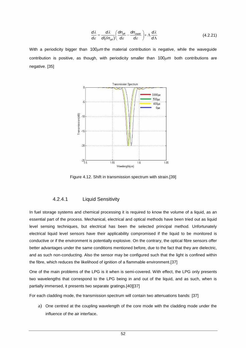
52

( )

eff cladd

eff

dn dnd d d

d d n d d d

(4.2.21)

With a periodicity bigger than 100 m the material contribution is negative, while the waveguide

contribution is positive, as though, with periodicity smaller than 100 m both contributions are

negative. [35]

Figure 4.12. Shift in transmission spectrum with strain.[39]

4.2.4.1 Liquid Sensitivity

In fuel storage systems and chemical processing it is required to know the volume of a liquid, as an

essential part of the process. Mechanical, electrical and optical methods have been tried out as liquid

level sensing techniques, but electrical has been the selected principal method. Unfortunately

electrical liquid level sensors have their applicability compromised if the liquid to be monitored is

conductive or if the environment is potentially explosive. On the contrary, the optical fibre sensors offer

better advantages under the same conditions mentioned before, due to the fact that they are dielectric,

and as such non-conducting. Also the sensor may be configured such that the light is confined within

the fibre, which reduces the likelihood of ignition of a flammable environment.[37]

One of the main problems of the LPG is it when is semi-covered. With effect, the LPG only presents

two wavelengths that correspond to the LPG being in and out of the liquid, and as such, when is

partially immersed, it presents two separate gratings.[40][37]

For each cladding mode, the transmission spectrum will contain two attenuations bands: [37]

a) One centred at the coupling wavelength of the core mode with the cladding mode under the

influence of the air interface.

53

b) The other with the coupling wavelength of the core mode to the same cladding modes under

the influence of refractive index of the liquid.

By using the equation above, we can represent the minimum transmission value of the attenuation

bands a) and b). With an LPG of the length L, immersed in the liquid l the attenuation band a) AT and

b) BT , the equations are: [37]

2sin

2A

lT

L

(4.2.22)

2sin

2B

L lT

L

(4.2.23)

The figures below demonstrate the influence on the transmission of an LPG dipped in air and water.

Figure 4.13. The spectra of the mobile liquid level sensor with a 1,546.25-nm resonance

wavelength LPG.[49]

4.3 Production of Chiral Fibre Gratings

As we explained before, chiral fibre gratings are not built the same way as the pure chiral fibre. In

order to construct this chiral fibre gratings it is used glass fibres with cores that are either concentric

and birefringence or no-centric. Afterwards they are twisted at a high rate as they are passed through

a miniature oven in a drawing tower. Depending on the direction of the motor rotation the structure is

right-handed or left-handed.[24]

This innovation permits the fabrication of a stable structure, which has double-helix symmetry, e.g.

twisted concentric birefringence fibres, or single-helix symmetry, e.g. twisted no-centric fibres. In

double-helix structures, resonance interactions only occur for co-handed circularly polarized light with

54

the same handedness as the structure. This type of fibre is more useful as polarizer. While in single-

helix structures with no-birefringence cores, resonance interactions are polarization insensitive. This

structure has, however, the potential to be used as a sensor for temperature, strain and liquid

level.[24]

Figure 4.14.Twisted birefringent optical fibre. [50]

4.4 Groups and types of Chiral Fibre Gratings

Chiral optical fibre gratings can be organized in three groups, depending on the range between each

pitch i.e. /i

P Q and it can also be sub-divided in two types, double-helix and single-helix.

Considering for now, the sub-type double-helix, it can be organized in the following three groups of

chiral fibre gratings, as mentioned above.[24]

Chiral short-period grating (CSPG): Where the pitch equals to the optical wavelength in the

order of 1 m that reflects light within the fibre core.

Chiral intermediate-period grating (CIPG): With a pitch order of 10 m , the light scatters out of

the fibre.

Chiral long-period grating (CLPG): With a space pitch’ of the order of 100 m , it couples core

modes into co-propagating cladding optical modes.

Considering the /i

Q P with 1Q , the CSPGs reflect co-handed light within the fibre core within a

stop band corresponding to a range of wavelength within the fibre. Diversely cross-handed light of the

orthogonal polarization is freely transmitted. These fibres are used as polarization selective spectral

filter with a bandwidth relative to the band centre wavelength equal to the fractional fibre

birefringence.[24]

In the case of the CIPG, where the ratio is 1 100Q , light scatters out of the fibre, however, only co-

handed light is scattered near the edges of the band. Due to this characteristic, this type of technology

may serve as polarization and wavelength selective filters.[24]

Finally the CLPG, with 100Q , couple core modes into co-propagation cladding optical mode when

the difference between the propagation constant of the core and various cladding modes is

compensated by the grating. These type of fibres serve better for sensing pressure, temperature and

55

liquid fluid level, [24] but it can also work as a polarizer.[44]

The figure below represents the behaviour of a double-helix chiral fibre grating of three groups

mentioned above, i.e. indicates the variation of ration of right-to-left circularly polarized transmission

with the values of Q.[24]

Figure 4.15. Performance of a double-helix chiral fibre grating giving the ratio of right to left circularly

polarization vs /i

Q P .[24]

From the analyses of the figure above, we can infer that small values of Q transmits LCP light, which

was acquired for a microwave transmission through a chiral rod, as in the bigger values of Q only LCP

propagates through the core and the RCP goes through the cladding (values that were obtained for

infra-red radiation in the telecommunication range). However it is notable the scattering of the light

between the values of log( ) 1Q and log( ) 1.65Q , even though in the edges only RCP is scattered.

In sum, we may infer that, with expectation of the edges, the values between this gap is insensitive to

polarization, and as though all light is scattered.[24]

Since single-helix structures are polarization insensitive, none of the groups presented above

indicated any special feature, which behaviour is similar to a fibre Bragg gratings and long period

gratings.[24]

4.5 Chiral Long Period Gratings

On this subchapter we will present the performance of CLPG and the differences between those of

single-helix and double-helix. As we demonstrated before, double-helix structures are sensitive to

polarization, as contrary to single-helix structures.[40]

56

4.5.1 Double-helix

In general to construct a double-helix structure, we must use low temperature glasses that are passed

through a short heat zone of length approximately of 300 m at a temperature above the softening

point. The heating element is an omega-shaped resistive wire. This type of fibre has a refractive index

of the core of 1.7 and a cladding of 1.5. Also the double-helix fibres have a birefringence of 0.03,

which is bigger than the corresponding values of the index of modulation that exists on photosensitive

glasses. These type of fibre have proven to be polarization selective, which mimic the symmetry of

CLCs (Cholesteric Liquid-Crystal).[41][40]

Figure 4.16. Example of a double-helix chiral long period grating.[40]

4.5.1.1 Polarization

As we know polarizers have the power to eliminate undesirable light component of a first polarization

and permits a better light component of a second polarization to pass through the fibre. In order to

apply this technology the system requires one or more polarizers. Many of these are required in

electro-optical modulators and laser subsystems. [42]

Present polarizers (in-line and lens-based polarizers) have however disadvantages. In-line polarizer is

relatively expensive and hard to build. The lens-based polarizer interrupts the optical fibre, leading to

optical loss and undesirable reflection. Also the lens-based are much bigger than the fibres so it

requires more space to incorporate in the optical system. [42]

The double-helix chiral fibre gratings provide an in-line polarizer that does not interrupt an optical fibre,

does not require much space on the system, and has the power to operate with an unpolarised light

input.[42] Even though chiral long period gratings are more suitable as sensors and chiral intermediate

fibre gratings have more advantages as polarizer, CLPG can also work as a polarizer and also has the

capability to shape the polarization spectra of the signals passing through the fibre.[44]

4.5.1.2 Potential applications

Next, considering the theory above, we shall show some examples of potentials chiral fibres:

57

Figure 4.17. a) Side image and schematic of face image of a double-helix fibre. b) Transmission

spectra of a double-helix. [43]

The figure 4.17.a) is a twisted custom fibre with rectangular core, having double-helix symmetry. To

produce this fibre is necessary to twist it to a uniform helical pitch of 78 m with a length of 55mm .

We verify that the polarization selectivity is demonstrated in the ratio of right circularly polarization

(RCP) to left circularly polarization (LCP) transmission. [43] By analysing the figure 4.17.b) we verify

that as wavelengths develops, the dip gets bigger, whereas with 1500nm wavelength, we obtain

2dB of transmission, with1650nm of wavelength and transmission of 25dB .These sharp spectral

dips indicate that the right-handed structure resonantly couples the RCP core mode to an LCP

cladding mode.

Figure 4.18. a) Side image and schematic of face image of a double-helix fibre. b) Transmission

spectra of a double-helix. [43]

The fibre from the figure 4.18.a) is constructed by twisting a conventional polarization maintaining

PANDA fibre after the fibre cladding was selectively imprinted to produce a cross section in the shape

of a figure eight of 2.5 m in diameter. This fibre must have a 20mm long air-clad structure

composed of a 8mm long portion with uniform 16 m pitch and two twist acceleration and deceleration

portion with a distance of each other of 6mm long. Also this fibre efficiently couples the co-handed

58

light polarization component into free space while freely transmitting the orthogonal polarization. This

fibre serves as the basis for flexible, broadband, high extinction ratio in-fibre, linear and circular

polarizer. [43]

4.5.2 Single-helix

Overall single-helix structures are built in silica glass fibres and have the same procedure of

construction as double-helix structures, with the exception of the heat source, for which is used power-

stabilised focused 2CO laser. The single-helix CLPG have normally an index core of 1.48 and

cladding of 1.45. Firstly, these fibres have an off-centre elliptical core as we can observe on the figure

4.19.[41][40]

These types of chiral fibres are insensitive to polarization, and as such are more suitable for strain,

temperature and liquid level sensing. [40]

Figure 4.19. Example of a single-helix chiral long period grating. [40]

4.5.2.1 Liquid level sensing

One of the many functions of CLPG is the power to sense liquid level, as a normal long period grating.

As it occurs in LPGs, the light transmission at the wavelength located at the edge of the transition dip

is affected by liquid level. Both in LPG and CLPG, the transmission spectrum is shifted when the fibre

is completely submerged in liquid. However, as we explained on subchapter 4.2.4, LPG only presents

two results (wavelengths), respectively when it is submerged in liquid and when it is out of the liquid.

On the contrary, the CLPG gives us information even when the fibre is only partially covered in liquid.

As the level of the liquid changes, the dip shifts, continuously, without change in linewidth, as we can

see on the figure 4.20. [40]

59

Figure 4.20. Behaviour of CLPG transmission dips of single-helix covered with alcohol at different

heights.[40]

4.5.2.2 Temperature sensing

As we know, single-helix CLPGs are built with high temperature silica fibre, in other words, these

fibres have the capability to endure high temperatures, making them desirable as high-temperature

sensors. On the article [40] it was used the device, Micron Optic fibre interrogator, in order to study the

long term temperature stability and temperature sensitivity, in the temperature range 400-1100ºC. The

figure 4.21 indicates the dip wavelength vs the temperature. [40]

Figure 4.21. CLPG versus temperature, wavelength of transmission dip of single-helix.[40]

The figure above show us that the dip wavelength shifted 40nm from 50º to 500ºC. Also by observing

the figure 4.22 we verify that the sensitivity is 0.11 /ºmm C with 400 ºC. Furthermore analysing the

figure 4.22 the shift is stable at a given temperature, even after repeating the cycle.

Finally the figure mentioned before reveals a fluctuation that is characterize by slight curves on a few

temperatures, not reflecting drastic fluctuations. [40]

60

Figure 4.22. CLPG versus temperature, wavelength of transmission dip of single-helix.[40]

4.5.2.3 Potential Applications

Following, we will present some single-helix CLPG that are being presently produced:

Figure 4.23. a) Side image and schematic of face image of a single-helix fibre. b) Transmission

spectra of a single-helix.[43]

The figure 4.23.a) presents a single helix structure mode of a custom fibre with an off-centre core. This

chiral fibres is constituted with a 17mm long structure twisted to a pitch of 460 m . As we can see on

figure 4.23.b), this fibre is polarization insensitive and couples light of both polarization to cladding

modes. Also from the spectrum of the figure 4.23.b), we verify the polarization insensitive by the

independence of the transmission spectrum upon input polarization.[43] Doing a thoroughly analysis

on the figure 4.23.b) we see that the transmission starts with a value of 2dB , never going to 0dB ,

and as the wavelength progresses it starts to appear dips, which drifts becomes higher as the

wavelength grows, being the biggest dip at 1560nm with 22dB .

These fibres are useful for applications that need temperate sensing up to 600oC .[43]

61

Figure 4.24. a) Side image and schematic of face image of a single-helix fibre. b Transmission spectra

of a double-helix.[43]

The fibre represented in the figure above, was built in order to be compatible with conventional single-

mode fibres. It is produced by co-twisting a standard fibre with a scaffolding fibre, which its mission is

to implement a helical structure into the main signal fibre. To produce this fibre it is necessary that a

30nm long grating be twisted to a 1565 m pitch. By analysing the figure 4.24.b) we verify a single

polarization insensitive resonant dip in the spectrum. Also in the spectrum, transmission is equal for all

input polarization and the state of polarization is not preserved. [43] On the figure 4.24.b) there is only

one deep dip, with a wavelength 1550nm and a transmission of 17dB .

Figure 4.25. a) Side image and schematic of face image of a single-helix fibre. b) Transmission

spectra of a double-helix.[43]

The fibre from the figure 4.25.a) was produced from a microstructure fibre with a hexagonal

arrangement of holes; also this fibre is wholly made of pure silica and does not rely on glass doping to

build a core with increased refractive index relative to the cladding. [43] By observing the figure 4.25.b)

we see that the transmission starts with 5dB , begins ascending until a wavelength of 1515nm and

then it descends to 35dB of transmission on a wavelength of 1545nm . Afterwards, at 1555nm ,

62

surges another dip, less deep than the previous ( 36 )dB , followed of another rise, that reaches 5dB ,

stabilizing there.

4.6 Economical Perspective

Until now, we have seen the advantages of the chiral fibre gratings in comparison with the actual

technologies used in telecommunication, however we must also approach it from an economical

perspective.

On the table 4.2 we present the cost of several in-line (in-fibre) fibre optical polarizers, sold nowadays

in the following companies: Chiral Photonics [45], company that produces chiral fibres, Thorlabs [46]

and Newport, which production is dedicated to normal polarizers [47].

Chiralphotonics Thorlab Newport

IFP980PM-FC € 348 ILP980PM-FC € 278

IFP1064PM-FC € 348 ILP1064PM-FC € 302

IFP1310PM-FC € 348 ILP1310PM-FC € 284 F-ILP-1-F-SP-FP € 367

IFP1550PM-FC € 348 ILP1550PM-FC € 284

IFP1550SM-FC € 331 ILP1550SM-FC €207,90 F-ILP-2-F-SS-FP € 263

Table 4.2. Purchase cost of several in-line fibre polarizers.

On a first analysis we verify that, in comparison with the three companies polarizers, Chiral Photonics

presents the most expensive polarizers with the exception of F-ILP-1-F-SP-FP polarizer, which

belongs to the Newport company. The Thorlab polarizers show the cheapest polarizers in comparison

with the rest of the companies. Also, all of the polarizers of Thorlabs are less expensive than Chiral

photonics, in order of 70€ (IFP1550SM-FC - ILP1550SM-FC ) to 123.1€ (IFP980PM-FC - ILP980PM-

FC). In comparison with Chiral photonics and Newport, IFP1310PM-FC it is less expensive (19€) than

F-ILP-1-F-SP-FP, however IFP1550SM-FC it is more expensive (68€) than F-ILP-2-F-SS-FP.

From all this we can conclude that, notwithstanding the innovation brought with chiral fibre gratings,

its economic cost are still too elevated in comparison to the normal polarizers, making it, in my

opinion not yet sufficiently viable to replace the actual polarizers.

Regarding the sensors, we have found one built from the Chiral Photonics –“HTS-1000 Ultra-high

Temperature Fiber Optic Temperature Sensor”, which cost is 550,74€ [48], however in our research, it

was not possible to find similar sensors and as thus ,we could not make a comparison, between a

chiral and a normal sensor. Nevertheless, it is our believe that it is notable the high monetary cost of

acquisition of this product, due to is novelty.

63

4.7 Conclusion

In this chapter we presented a new type of chiral fibres, the chiral fibres gratings. Diversely, to the

pure chiral fibres that are constituted by chiral material, this new type of fibre is a normal glass fibre

that has cores which are either concentric and birefringence or no-centric. They are also twisted at a

high rate as they are passed through a miniature oven and accordantly to the way the motor rotations

is twisting, the structure is right-handed or left-handed. This extends their functionality to filters,

polarizers, sensors and laser applications.

In order to understand this innovation, we first explain its predecessors: the fibre Bragg gratings and

the long period gratings. Fibre Bragg Grating is a periodic perturbation of the refractive index in a

waveguide. By exposing the core of a single-mode fibre to a periodic pattern of a strong UV light, we

can fabricate FBG. This technique provokes a permanent index of refraction in the core of the fibre,

and it also makes the core behave as a selective mirror of wavelengths that satisfies the Bragg

condition. Long period grating consists on a periodic modulation of the refraction index in the core of

an optical fibre. The LPG has a typical period of 100 m to 1mm . This technology permits coupling

between fibre modes having similar propagation constants, for example, between the core-mode and

the cladding-mode.

In the other hand, chiral optical fibres can be divided in three groups, depending on the length of the

periods: chiral short period grating (CSPG), chiral intermediate period grating (CIPG), and long period

grating (CLPG). The CSPG reflects the co-handed light on the core, but the cross-handed light passes

without interruption through the fibre. This type of fibre is more used as selective spectral filter

polarizer. The CIPG scatters light through the core with exception on the edges of the band between

CSPG and CLPG, where only co-handed light is scattered. This fibre is more suitable as a polarizer

and a wavelength selective filter. Finally CLPG couples the guided mode (core-mode) with cladding

mode. This fibre is preferable as sensors of pressure, temperature and liquid fluid level, but it has

potential to work also as a polarizer. However the conclusions above only consider the double-helix

structures.

Indeed, these three groups can also be divided in two types of structures, double-helix and single-

helix. In order to produce a double-helix optical fibre it is used low temperature glasses, which are

passed through a short heat zone of length approximately of 300 m at a temperature above the

softening point. Also the heating element is an omega-shaped resistive wire. This type of fibre is more

suitable as polarizer and presents potentially more advantages than the present polarizers (in-line and

lens-based). In effect, nowadays, in-line normal polarizers have large monetary cost in terms of

production and are hard to build. Also, the lens-based polarizer interrupts the optical fibre, which

provokes optical losses and undesirable reflection, and it sizes requires more space to be introduced

in the optical system. In comparison, the double-helix chiral fibre provides an in-line polarizer that does

not interrupt the fibre, does not occupy much space on the system and finally has the capability to

function with an unpolarised light input.

64

As for single-helix optical chiral fibre, it is built as the double-helix but it uses a different heat source

(power-stabilised focused 2CO laser). This optical fibre even though is insensitive to polarization, is

useful for strain, temperature and liquid level sensing. As we stated on chapter 4.2.4, long period

gratings (LPGs) have the capacity to sense liquid, but unfortunately it only provides two results,

specifically when is in or out of the liquid. Chiral long period grating fortunately provides with

information even when it is partially covered in liquid. As the level of the liquid changes, the dip shifts

continuously. As for sensing temperature, as aforementioned, CLPG are constructed with high

temperature silica fibre, making it capable to endure high temperatures.

Finally, after studying the chiral fibre grating technology, we analysed these fibres from an economic

perspective, specifically by comparison with the nowadays devices (polarizers and sensors). It was

concluded that, notwithstanding the advantages from the technological point of view from the in-line

chiral fibre, it is still too expensive in comparison with the nowadays polarizers. As to the sensors, it

was not possible through our research to make a comparison with actual devices on the market,

however it is our opinion that the chiral sensor presents still a too high monetary cost.

65

Chapter 5

Conclusion

5 Conclusion

66

The main objective of this thesis is to analyse the chiral medium, specifically in telecommunications

area, through the pure chiral fibres (optical fibres constituted by chiral material) and chiral fibre grating

(twisted optical fibre). Besides others aspects, on this thesis we addressed the behaviour of those

fibres, as also theirs applications and its economic viability.

On the first chapter we presented the history of optical fibres and chiral fibres. Afterwards we

introduced the motivation and objectives of the thesis, its structure and its contributions.

On the second chapter we explained the meaning of chiral objects, which is the incapacity of an object

and its mirror image to be superimposed, whose capacity is defined by its power to rotate the plane of

linearly polarized light (optical activity), and as such marks it as belonging to the bi-isotropic group.

In order to clarify this definition we studied the constitutive relations of this medium using the Kong

model. Unfortunately, due to the difficulty to analyse the wave that passes through the bi-isotropic

medium, in order to overcome this problem, we divided into two waves (“plus” and “minus”) and

considered that they belong in an isotropic medium. With these waves, we studied their

characteristics, in order to determine their polarization and its rotation. With the polarization

determined, we concluded that circular polarization is only possible because of the medium being

circular birefringent i.e. when a wave passes through this medium it is split by polarization into two

waves. Later on, we introduced the laws of reflection and refraction of a wave that focus on the

boundary between a dielectric medium and a chiral medium. Finally we calculated the reflection and

transmission coefficients of the waves, to comprehend the power carried by reflected and transmitted

waves and also the polarization properties.

On the third chapter, we investigated the pure chiral fibre (optical fibre constituted by chiral material).

In order to understand the modes produced by this fibre we addressed it through the modal equation

that represents the chiral cladding and achiral core and also the chiral cladding and chiral core. With

this formulation it was possible to simulate the mode cut for surface and semileaky, dispersion

diagram and finally radiation loss of L and R mode. With chiral cladding and achiral core, on the

surface and semileaky mode cuts, we verified that on the surface mode cut it exists an asymptote (

1 2 2/v n n g ) and that above it, it stops existing the surface mode. Also we saw that the L type

have bigger slopes than the R type. Finally on semileaky mode only L type exists. On the dispersion

diagram it only exist one R type ( 01R ), which starts on 2.6v as surface until 12.3v , where it

becomes undefined (non-existent) and finally it ends as semileaky. All the L mode type starts as

semileaky and end as such, with the exception for 01L , which starts at 2.5v , turns surface at

2.7v and regresses semileaky at 11.5v . Also, by analysing the radiation loss figures we

concluded that R and L mode has positive slopes and the negative slopes, respectively.

On the subject of both chiral cladding and core, on the figures of the cut modes the L and R type

belong to the positive slope and negative slope, respectively. Considering the figure of the dispersion

mode we saw that the effective index of refraction ( )eff

n R type approached the p and the L type

approached the p . Furthermore with 12.5v the RCP is dominant on surface mode and LCP on

67

semileakys mode. On radiation losses only L type presents losses, where 01L has the biggest loss with

0.6 and 02L with 0.09 .

From the analyses of the both cases of the pure chiral fibre, we may infer that independently of the

core and cladding being both chiral or just the cladding, the phenomenon of the semileaky mode will

occur, as there will exist inevitably two characteristics waves. Nevertheless, on the fibre with an achiral

core and a chiral cladding the RCP is predominant and as such it will be semileaky. Diversely when

the fibre has both chiral cladding and core, the LCP is predominant and as such it will assume the

semileaky mode. However, in this last fibre, the semileaky mode on the L mode is frequently nullified,

as it occasionally couples with the R mode, commuting their characteristics. Through that occurrence

the L mode turns surface mode and the R temporarily semileaky mode, because it couples again with

another R, returning to its original mode (surface mode). In sum, the losses on the chiral fibre that has

both core and cladding chirality are fewer than on the fibre with only chiral cladding.

On the fourth chapter, we introduced a different type of chiral fibres fabricated by the company Chiral

Photonics. To produce this fibre, it is used glass fibres with cores that are either concentric and

birefringence or no-centric, then they are twisted at a huge speed at same time as they are heated on

a small oven in a drawing tower. These fibres are either right-handed or left-handed, depending on the

way the motor rotates. With this technology we are able to control the period on the optical fibres,

extending theirs functionality to filters, polarizers, sensors and laser applications.

Since these chiral fibres present some properties similar to fibre Bragg gratings (FBGs) and long

period gratings (LPGs), we begun by explaining these two technologies. FBG is a periodic

perturbation of the refractive index in a waveguide and we are able to produce this phenomenon by

revealing the core of the fibre to a strong UV light. This permits the FBG to behave as a selective

mirror of wavelengths that satisfies the Bragg condition. The LPG has the same method of fabrication

as FBG i.e. a periodic modulation of the index of refraction in the core. The period of the LPG is

around 100 m to 1mm and has the advantage to couple the core-mode and the cladding-mode.

After explaining the ancestors of the chiral fibres (chiral fibres gratings), we presented the groups and

types that they can be divided. These are sorted in three groups: chiral short period grating (CSPG),

chiral intermediate period grating (CIPG) and finally chiral long period grating (CLPG), and in each

group we can sub-divide in two types, double-helix and single-helix. On the CSPG, cross-handed light

goes freely through the fibre but the co-handed light is reflected on the core, and as such its more

suitable as a selective spectral filter polarizers. The CIPG scatters light through the core with the

exception on the edges of the band between CSPG and CLPG, where only co-handed light is

scattered, being more useful as a polarizer and a wavelength selective fibre. The CLPG couples the

core-mode with the cladding mode, being as such more useful as sensors of pressure, temperature

and liquid level, even though it has potential to be a polarizer. However the conclusions above only

consider the double-helix structures.

Afterwards, considering the sub-types of chiral fibre (double and single-helix), we disclosed that to

build a double-helix optical fibre it is necessary to use low temperature glasses, which are passed

68

through a short heat zone of length around of 300 m at a temperature above the softening point, and

the heating element is an omega-shaped resistive wire. This type of fibre present advantages as

polarizer in consideration with in-line and lens-based polarizers. This technology offers an in-line

polarizer that does not interrupt the fibre, does not require much space on the system and finally has

the capability to function with unpolarised light input.

The single-helix has the same procedure of construction as the double-helix, though it is used a

different heat source (power-stabilised focused 2CO laser). The single-helix has the power to sense

strain, temperature and liquid level. On the contrary of LPG, CLPG single-helix can inform us when it

is partially submerge in liquid i.e. as the level of the liquid changes the dip shifts continuously. As for

the temperature sensor, since the single-helix is produced at high temperatures, it has the capacity to

endure high temperature.

Finally, we approached the chiral fibres from an economical point of view, specifically its acquisition

cost, so that we could determine its monetary viability in comparison with the nowadays technology.

From the comparison between the costs of the polarizers, we concluded that the in-line polarizer chiral

fibres are more expensive than the actual in-line polarizers, making it less desirable to substitute the

actual polarizers. As to the sensors, it was not possible through our research to make a comparison

with actual devices on the market, however it is our opinion that the chiral sensor presents still a too

high monetary cost.

Nevertheless, it is undoubtable the technological breakthrough brought by this new technologic, even

though it is not yet viable technology (from an economic perspective) to replace the actual devices.

5.1 Future Works

After we concluded the objectives of this thesis we must consider other interesting topics that can be

addressed in future work:

Analyse couple-mode theory for chiral fibre gratings.

Investigate other purposes for chiral fibres.

69

Annex A

Constitutive Relations

Annex A. Constitutive Relations

In this section we are going to present a variety of model that represents the constitutive relations of

the chiral medium

71

A.1 Post-Jaggard model

This model was fist calculated by Post [10], which requires the covariant to be under the Lorentz

transformation.

Being the constitutive relation:

0 p pD E i B

(A.1.1)

0

1p

p

H B i E

(A.1.2)

Where the p

is the chiral admittance, p the permittivity and

p the permeability relative.

The relation between the Post Model and Kong model we acquire using the Eq. (2.213), Eq. (2.214)

and Eq. (A.1.1).

2

p

(A.1.3)

p

(A.1.4)

0pY

(A.1.5)

Or the inverse:

2

0( )

p p pZ (A.1.6)

p

(A.1.7)

0p p

Z (A.1.8)

A.2 Drude-Born-Fedorov model

This model, which had been analysed by Paul Drude [10], concluded that the rotation of the

polarization plane can be made with the introduction on polarization term mP proportional to E .

Through this model Born consider the constitutive relation:

0( )

D DD E E (A.2.1)

0 D

B H (A.2.2)

By observing the last equation we verify the non-local nature of the optical activity.

72

In order to make a connection of the parameter of this model with Kong model it is necessary to use

Maxwell equations for unsourced regions.

0( )

D DD E E (A.2.3)

0

( )D D

B H H (A.2.4)

Obtaining:

002 2

0 01D

D D

D D D

D E i

(A.2.5)

0

02 2

0 01D

D D

D D D

B H i

(A.2.6)

Acquiring:

2

D

(A.2.7)

2

D

(A.2.8)

2( )D

c

(A.2.9)

Or inversely:

2

2 2 2

D

D D D

c

c

(A.2.10)

2

2 2 2

D

D D D

c

c

(A.2.11)

2 2 2

D D D

D D D

c

c

(A.2.12)

73

References

References

[1] Kartalopoulos , V.S., Introduction To DWDM Technology. The Institute of Electrical and Electronics

Engineers, Inc.,USA: New York, 2000.

[2] Mitschke, F., Fibre Optics- Physics and Technology, Germany: Rostock, 2010.

[3] Paiva, C. R., Fotónica, Fibras Ópticas, DEEC, IST, 2008. [4] Cartaxo, A., Sistemas de Telecomunicações por fibra Óptica. Transmissão por Fibra Óptica, IST 2005. [5] A. Elsherbeni, V. Demir, M. A. Sharkawy, E. Arvas, S. Mahmoud, Electromagnetic Scattering From Chiral Media, Progress in Electromagnetic Research Symposium, Italy, Pisa, March 28-31, 2004. [6]J. Lekner, Optical Properties of Isotropic Chiral Media, Department of Physics, Victoria University of Wellington, Welligton, New Zealand, 1996. [7] D.L. Jaggard, A. R. Mickelson and C.H. Papas, On electromagnetic waves in chiral media, Division of Engineering and Applied Science, California Institute of Technology, Pasadena, CA 91125, USA, 21 August, 1978. [8] J. Lekner, Optical properties of isotropic chiral media, Department of Physics, Victoria University of Wellington, New Zealand, January 1996. [9] P. D. G. Dessai, Influence of Chirality on the Electromagnetic Wave Propagation: Unbounded Media And Chirowaveguides, Instituto Superior Técnico, Portugal, Lisboa, Dezembro, 2011. [10] F.M. Janeiro, Quiralidade e Não-Linearidade em Fibras Ópticas, Instituto Superior Técnico, Portugal, Lisboa, 2004. [11] M. H. Winkler, “An experimental investigation of some molecules for optical activity”, Journal of Physical Chemistry, vol. 60, pp. 1656-1659, 1956. [12] J. A. Kong, Electromagnetic Wave Theory, New York, Wiley, 1986. [13] P. Pelet and N. Engheta, “Theory of chirowaveguides”, IEEE Trans-actions on Antennas and propagation, vol. 38, no.1, January 1990. [14] J. B. Pendry, A New Route to Negative Refraction, Department of Physics, The Blackett Laboratory, Imperial College London, London SW72AZ, UK, August 13, 2004. [15] C. R. Paiva, Meios Quirais e Actividade Optica, Departamento de Engenharia Electrotecnica e de Computadores, IST, Março 2007. [16] S. Bassiri, Electromagnetic Wave Propagation and Radiation in Chiral Media, California Institute of Technology, Pasadena, California, February 4, 1987. [17] Mitschke, F., Fibre Optics- Physics and Technology, Germany: Rostock, 2010. [18] Paiva, C. R., Fotónica, Fibras Ópticas, DEEC, IST, 2008.

74

[19] Pires, J., Fibras Ópticas, IST, 2003. [20] F. M. Janeiro, C.R. Paiva, Analysis of Surface and Semileaky Modes in Chiral Optical Fibers Using the Condon Model to Account for Dispersion in Optically Active Media. Departamento de Física, Universidade de Évora, Évora, Portugal, Setembro, 2004. [21] F. M. Janeiro, C.R. Paiva, A. L. Topa, Guidance and leakage properties of chiral optical fibers, Instituto de Telecomunicações, Instituto Superior Técnico,30 Abril, 2002. [22] L. Poladian, M.Staton, A. Docherty, A. Argyros, Pure chiral optical fibres, Institute of Photonics and Optical Science (IPOS), School of Mathematics and Statistics, The University of Sydney, NSW 2006, Australia, Institute of Photonics and Optical Science (IPOS), School of Physics, The University of Sydney, Australia, NSW 2006. [23] V. I. Kopp, V. M. Churikov, A. Z. Geneack, Chiral-fiber gratings: sense the environment, January 06, 2008. [24] A. Méndez, T. F. Morse, Specialty Optical Fibers Handbook, 2007. [25] Ou, W, W, L., Fiber Bragg Grating Strain Sensors for Railway Applications, B.Eng., University of Auckland, 2006. [26] Zhao, J. ,Thesis on An Object-oriented Simulation Program for Fibre Bragg Gratings, Rands Afrikaans University, Johannesburg, Republic of South Africa, October 2001. [27] Shing, C. C., An investigation of chirped fibre Bragg gratings Fabry-Perot interferometer for sensing applications, Cranfield University, USA, Cranfield, March 2005. [28] Vieira, A. M. A.,Compensação de dispersão em Sistemas de Fibras Ópticas, Instituto Superior Técnico, Portugal, Lisboa, Abril, 2014 [29] Low Cost Fiber Bragg Grating (FBG) Sensors for Structural Health Monitoring, June 11, 2011. [30] Shing, C. C., An investigation of chirped fibre Bragg gratings Fabry-Perot interferometer for sensing applications, Cranfield University, USA, Cranfield, March 2005. [31] Yariv, A., Yeh, P., Photonics Optical Electronics in modern communications, sixth edition, Oxford University Press, USA, New York, 2007. [32] Nogueira, R. N., Redes de Bragg em fibra óptica. Universidade de Aveiro, Departamento de Física, Portugal, Aveiro, 2005. [33] Aulakh, N. S., Investigations on Fiber Bragg Gratings for Fiber Optic Communication Systems, Department of Electronics & Communication Engineering, Thapar University, India, Patiala, 2010. [34] V. Bhatia, Properties and Sensing Applications of Long-Period Gratings, Virginia Polytechnic Institute and State University, Blacksburg, Virginia, November, 1996 [35] S.W. James, R. P. Tatam, Optical fibre long-period grating sensors: characteristics and application, Cranfield University, Cranfield, Bedford, MK43 OAL, UK, 2003. [36] V. Bhatia, Applications of long-period gratings to single and multi-parameter sensing, Optical componentes development, Science and Technology, Corning Incorporated, SP-DV-01-6, Corning, New York 14831, May 21, 1999. [37] S. W. James, S. Khaliq, R. P. Tatam, A Long Period Grating Liquid Level Sensor, Optical sensors, group, centre for photonics and optical engineering, School of engineering, Cranfield University, Cranfield, Bedford, MK43 OAL, UK, 2002.

75

[38] S. Chaubey, P. Joshi, M. Kumar, R. Arya, A. K. Nath, S. Kher, Design and development of long-period gratings sensors for temperature monitoring, Fibre Optics Lab, SSLD, Solid State Laser Division, Raja Ramanna Centre for Advanced Technology, Indore 450 213, India, 17 August 2006. [39] A. Sharma, D. Engles, A. Singh, Study of Long Period Grating as Strain Sensor, Department of Electronics Technology, G.N.D.U. Amritsar, June 2012. [40] V. I. Kopp, V. M. Churikov, G. Zhang, J. Singer, C. W. Draper, N. Chao, D. Neugroschl, A. Z. Genack, Single- and double-helix chiral fiber sensors, Chiral Photonics, Inc., Clifton, New Jersey 07012, USA, August 8, 2007. [41] V. I. Kopp, A. Z. Genack, Chiral fibres: Adding twist, 2011. [42] V. I. Kopp, United States Patent: 7.095.911, August 22, 2006. [43] V. I. Kopp, J. Park, M. Wlodawski, J. Singer, D. Neugroschl, A. Z. Genack, Chiral Fibers: Microformed Optical Waveguides for Polarization Control, Sensing, Coupling, Amplification, and Switching, Chiral Photonics, 2013 [44] V. I. Kopp, United States Patent: 6.925.230, August 02, 2005. [45] On site - http://www.thorlabs.com/catalogpages/V21/1132.pdf. [46] On site - http://www.thorlabs.com/newgrouppage9.cfm?objectgroup_id=5922. [47] On site – http://search.newport.com/i/1/x1/pageType/q1/Products/q2/Fiber%20Optics/q3/Polarization%20Components/q4/Fiber%20Optic%20In-Line%20Polarizers/x2/section/x3/chapter/x4/family/nav/1/ [48] On site - http://www.chiralphotonics.com/Web/default.html. [49] J. N. Wang, C. Y. Luo, Long-Period Fiber Grating Sensors for the Measurement of Liquid Level and Fluid-Flow Velocity, Department of Construction Engineering, National Yunlin University of Science and Technology, Douliou 64002, Taiwan, 30 December 2011. [50] V. I. Kopp, V. M. Churikov, Synchronization of optical polarization conversion and scattering in chiral fibers, Chiral Photonics, Inc., Clifton, New Jersey 07012, October 10, 2005. [51] L. M. P. C. C. Marques, Dissertação sobre Compensação de Dispersão em Sistemas de Fibra Óptica, Instituto Superior Técnico, Portugal, Lisboa, Outubro 2012.

76