Child Benefits and Macroeconomic Simulation Analyses … · Child Benefits and Macroeconomic...
28
Policy Research Institute, Ministry of Finance, Japan, Public Policy Review, Vol.9, No.4, September 2013 633 Child Benefits and Macroeconomic Simulation Analyses : An Overlapping-Generations Model with Endogenous Fertility Kazumasa Oguro Hosei University Junichiro Takahata Dokkyo University Abstract In predicting the impact of policies on macroeconomic variables, the government must consider the effect of household fertility choices on demographic trends, as macroeconomic variables can be influenced by population scale. Therefore, this paper presents a comprehensive survey of existing studies with endogenous fertility models and examines the effect of various policies on macroeconomic variables through simulation analysis based on the overlapping generations model (OLG) of Oguro et al. (2011), which determines population growth endogenously, with the growth rate affected by household fertility choices. Our results demonstrate a major effect on future population and public debt predictions studied in a scenario combining fiscal reform and introduction of child benefits. Keywords: overlapping generations model, child benefits, endogenous fertility JEL Classification: C68; D9; E62; H5; H6; J13 1. Introduction Decreasing birthrates coupled with an aging population, progressively seen in Japan and many other advanced countries, are causing demographics to change. Such changes affect not only public finance and social security, but also macroeconomics as a whole. However, fertility choice, one example of individual decision-making, is influenced by the environment enveloping that process. Here, the focus is on the effect child benefits (such as the child allowance) have on macroeconomics. By this we mean that the pay-as-you-go public pension system comes with a birth rate externality triggering incentives for a “free ride” for children of other families, ultimately lowering birth rate from the socially optimal value. The child allowance is one policy that internalizes this externality. Moreover, this internalization may possibly be implemented by both policies, increasing pensions— depending on the fertility rate—as well as child allowance, both theoretically equal. Therefore, if pay-as-you-go public pension has a mechanism reducing the fertility rate, to what degree would a child allowance expansion improve the fertility rate? Answering this question requires an exhaustive and judicious
Transcript of Child Benefits and Macroeconomic Simulation Analyses … · Child Benefits and Macroeconomic...

Policy Research Institute, Ministry of Finance, Japan, Public Policy Review, Vol.9, No.4, September 2013 633
Child Benefits and Macroeconomic Simulation Analyses : An Overlapping-Generations Model with Endogenous Fertility
Kazumasa OguroHosei University
Junichiro TakahataDokkyo University
Abstract
In predicting the impact of policies on macroeconomic variables, the government must consider the effect of household fertility choices on demographic trends, as macroeconomic variables can be influenced by population scale. Therefore, this paper presents a comprehensive survey of existing studies with endogenous fertility models and examines the effect of various policies on macroeconomic variables through simulation analysis based on the overlapping generations model (OLG) of Oguro et al. (2011), which determines population growth endogenously, with the growth rate affected by household fertility choices. Our results demonstrate a major effect on future population and public debt predictions studied in a scenario combining fiscal reform and introduction of child benefits.
Keywords: overlapping generations model, child benefits, endogenous fertilityJEL Classification: C68; D9; E62; H5; H6; J13
1. Introduction
Decreasing birthrates coupled with an aging population, progressively seen in Japan and many other advanced countries, are causing demographics to change. Such changes affect not only public finance and social security, but also macroeconomics as a whole. However, fertility choice, one example of individual decision-making, is influenced by the environment enveloping that process. Here, the focus is on the effect child benefits (such as the child allowance) have on macroeconomics.
By this we mean that the pay-as-you-go public pension system comes with a birth rate externality triggering incentives for a “free ride” for children of other families, ultimately lowering birth rate from the socially optimal value. The child allowance is one policy that internalizes this externality. Moreover, this internalization may possibly be implemented by both policies, increasing pensions— depending on the fertility rate—as well as child allowance, both theoretically equal. Therefore, if pay-as-you-go public pension has a mechanism reducing the fertility rate, to what degree would a child allowance expansion improve the fertility rate? Answering this question requires an exhaustive and judicious
634 K Oguro, J Takahata / Public Policy Review
“empirical analysis,” for which two predominant methods exist.One method is econometric analysis. Normal econometric analysis assumes a function in
which the birth rate = f (child allowance, income, etc.) to analyze increases in birth rate based on a child allowance expansion using past time-series data. This method clarifies the influence a child allowance expansion wields on the birth rate.
Although the importance of econometric analysis is accepted, the method may be lacking from an economics perspective. Policy merits are generally compared by evaluating the utility of the economic entity. To simplify the discussion, let us consider an economy in which the youthful generation (20 years and younger) is comprised of 1 person, the working generation includes 3 persons, and the retired generation is represented by 1 person. In this economy, only the working generation is a “productive population”; the retired and youthful generations are both dependent populations and each person in the working generation performs 100 units of productivity. In this scenario, as the productive population is 3 and the dependent population 2, the average individual share of the “economic pie” is 60 (100×3÷5). On the other hand, as child allowance expansion increases the youthful generation from 1 to 2 people, the dependent population rises to 3, decreasing the average share of the pie to 50 (100×3÷6). In other words, as the birth rate improves, the dependent population increases, possibly causing a temporary reduction in the economic entity utility. However, in the mid- to long-term, the youthful generation (20 years and younger) will mature and join the labor market, increasing the productive population. This should increase the average pie share per person, possibly increasing the economic entity utility for the mid- and long-term. This scenario also promises enhanced mid- to long-term public and public pension financing generated by increased tax revenue and social insurance premiums. Yet such econometric analysis is limited as the influence of child allowance on the economic entity utility differs by generation. This is where a second type of empirical analysis—namely, simulation analysis— comes into play.
This paper uses simulation analysis to clarify the influence of child benefits, pension reform, and fiscal reform on macroeconomics as well as on current and future generations. To do so, we apply the general equilibrium Overlapping Generations Model (OLG model) constructed by Oguro, Takahata and Shimasawa (2011). Before discussing the analysis, we would like to touch upon the issue of the most desirable method of funding for child benefits.
This topic is important, as selecting the financial resources to cover the cost of child benefit expansion is a problem unique to the OLG model with endogenous fertility, and does not affect the OLG model with exogenous fertility. As a result, the influence exerted on the utility of current and future generations will vary according to the financial resources selected to fund child benefits.
For the sake of comparison, let us examine existing studies involving the OLG model with exogenous fertility.
For the standard OLG model represented by Diamond (1965) and others, it is well established that consumption taxation (VAT) is the most effective method to raise financial resources for the welfare of future generations, followed by wage taxation and capital income taxation, the second and third methods of choice, respectively, given the future path of

Policy Research Institute, Ministry of Finance, Japan, Public Policy Review, Vol.9, No.4, September 2013 635
government expenditure. This can be explained as follows.The first benchmark is the theorem of zero taxation of capital income, derived from
Atkinson and Stiglitz’s (1976) theorem of optimal tax. The theorem is best understood by considering the OLG model with two generations, working and retired, living concurrently. At the first period (working period), each generation earns wage income by providing labor force, consumes a part of that income, and saves the remainder. At the second period (retired period), the retired generation consumes the principal and the interest derived from that saving. In this setting, Atkinson and Stiglitz (1976) have proved that the case in which the consumption tax of the first period is different from that of the second period is not optimal. In addition, since these respective differing consumption taxes have the taxation property for the interest on the savings consumed in the retired period, this theorem suggests that zero taxation of capital income is optimal; it holds in the OLG model with multi-concurrent generations and exogenous fertility.1 Similarly, Chamley (1986) and Judd (1985) also indicate that zero taxation of capital income in the OLG model with exogenous fertility and taking over inheritance among generations is most effective in the long term.
Moreover, on the steady state, the equation (1 – wage tax rate) × (1 + consumption tax rate) = 1 holds and consumption taxation becomes equivalent to wage taxation with no borrowing constraint and no change in government policies. Because of this, a switch in government policies from wage-based to consumption-based taxation, if implemented at a tax rate equivalent to that described previously, may have no influence on the generation immediately after the policy change, but the effect during the transition period may differ. Taxation on the retired generation’s consumption in the early stage of the transition period presents less distortion as it works like a lump-sum tax. In other words, considering intertemporal government budget constraints with the zero-sum feature of intergenerational income transfer, this policy would result in a transfer of income from the retired generation to the working and future generations.
An increase in the public debt tends to instigate the crowding-out effect, which may lead to a restrained accumulation of capital and a decrease in future economic growth. In the same manner, according to Hatta and Oguchi (1999), among others, the pay-as-you-go public pension also carries an “implicit debt” of approximately 150% of GDP and may inhibit future growth. Although public pensions transfer income from the working and future generations to the retired generation, implementation of the above-mentioned policies would have the opposite effect, transferring the income from the retired generation to the working and future generations, resulting in an increase in capital accumulation and enhanced future growth.
From this we can infer that, in the standard OLG model with exogenous fertility and given the future path of government expenditure, consumption taxation (VAT) would most often be the optimal source of funding for expenditure, followed by wage taxation and capital income taxation, in that order. However, as the assumptions in the OLG model with exogenous
1 The reader should remember that Atkinson and Stiglitz’s (1976) partial equilibrium analysis greatly influences the optimal tax rule, while considering the OLG model with exogenous fertility based on the evaluation criteria of the growth process known as the “Golden Rule.”
636 K Oguro, J Takahata / Public Policy Review
fertility are realistically modified, the conclusions drawn—such as the theorem of zero taxation of capital income—begin to differ.
For example, Cremer and Gahvari (1995) indicated that if the wage income in the second (retired) period is uncertain, it is desirable that the taxation imposed on the second-period consumption is higher than that of the first (working) period. This means that capital income taxation is desirable.
Similarly, Conesa et al. (2007) suggest that, when life expectancy and wage income are uncertain, a capital income tax is desirable. Saez (2002) adds that zero capital income taxation is not always optimal, as the desirable savings rate differs with varying levels of individual skill. Moreover, Weinzierl (2007) shows that, when wage income varies with age and there are heterogeneous demographics, a 15% tax would increase social welfare more than the zero-taxation scenario. In addition, Hubbard and Judd (1986) found that, when the capital market is incomplete and there are borrowing constraints, the implementation of capital income taxation can be justified.
As described above, modifications by Atkinson and Stiglitz (1976) suggest that there are various justifications for the implementation of capital income taxation. However, these are based on the OLG model with exogenous fertility; research on the justification of capital income taxation, assuming the OLG model with endogenous fertility, remains insufficient. Our results show that the child-rearing cost is the key parameter in the OLG model with endogenous fertility. For example, zero capital income taxation may no longer be considered optimal if the child-rearing cost is an increasing function of lifetime income. This can be explained as follows. First, zero capital income taxation is desirable in the standard OLG model with exogenous fertility; however, in comparison to nonzero capital income taxation, both lifetime income and child-rearing costs increase for future generations. If the positive effect of increased lifetime wages is overshadowed by a larger negative effect of increased child-rearing costs, the relative value of lifetime wages for child-rearing costs decreases due to the lifetime budget constraints of each generation. In such a case, although the implementation of capital income taxation is in fact justified, research based on the OLG model with endogenous fertility is not being pursued.
On the basis of the findings of Oguro et al. (2009), we construct an OLG model with multi-concurrent generations and endogenous fertility, assuming consumption, wage, capital, and other taxations as potential funding sources for increased child benefits, to analyze the effect on the welfare of each generation. We then analyze the effect on the welfare of each generation from the perspective of future social security reforms in two hypothetical cases: reducing pension benefits and using consumption tax to partially fund pension benefits.
According to our simulation results, the welfare for the future generation in the case with child benefits expansion funded by capital income tax is greater than in the case with child benefits expansion funded by consumption tax. This indicates that zero taxation of capital income in the OLG model with endogenous fertility is not the most effective in the long term.
Our research is organized as follows. In Section 2, we survey an OLG model with endogenous fertility. In Section 3, we explain the OLG model with multi-concurrent

Policy Research Institute, Ministry of Finance, Japan, Public Policy Review, Vol.9, No.4, September 2013 637
generations and endogenous fertility used in this paper. In Section 4, we describe the data, as well as the calibration and simulation scenarios used in our research. In Section 5, we evaluate the simulation results. Finally, in Section 6, we summarize our results and suggest topics for future discussion.
2. Survey on an OLG Model with Endogenous Fertility
In this section we introduce existing studies with endogenous OLG models, which determine the population growth rate endogenously. To do so, we first present classic OLG models and the issues they present, followed by OLG models with endogenous population growth, concluding with a case which introduces information asymmetry.
(1) From exogenous to endogenous population growth
The model with an endogenous population growth rate involves a mechanism in which the number of births selected by each household based on certain motivations is reflected in the population growth rate of the entire economy. As the population growth rate is determined, the population of the following period is revised, affecting per capita capital. Therefore, the population growth rate wields influence on the conditions for optimal consumption in the economy, just as it is affected by the amount of household savings.
The OLG model related to an exogenous population growth rate has been widely used for analysis since studies emerged by Samuelson (1958) and Diamond (1965). Samuelson (1958) maintains that each generation can sufficiently prepare for retirement without public pensions if money is available whose rate of return is equivalent to the population growth rate. Diamond (1965) goes on to argue the theory, stressing the “Golden Rule” of capital accumulation. In the OLG model, as individual household savings are not optimal for the economy as a whole, a capital savings level maximizing per capita consumption can be achieved through measures such as the issuance of government bonds. This capital savings level is stipulated if the economic growth rate—the sum of the population growth rate and the technical progress rate—and the interest rate become equal, a condition often referred to as the “Golden Rule.”
For instance, when the economic growth rate is lower than the interest rate, the latter can be lowered to narrow the gap by increasing current generation consumption with a bond issuance, resulting in an enhanced welfare level for all generations. In this sense, initial resource allocation was dynamically inefficient. Conversely, with an economic growth rate higher than the interest rate, the existing public debt (i.e. bonds) can be reduced to increase per capita consumption for current and future generations. This would, however, call for a tax increase on the current generation, which cannot improve the welfare of a specific generation without lowering the welfare of the others. In this sense, initial resource allocation was dynamically efficient.
Samuelson (1975) discussed levels of optimal population growth rate in this type of OLG model with an exogenous population growth rate, where per capita consumption varies with

638 K Oguro, J Takahata / Public Policy Review
the population growth rate. Although this research uses a model that does not allow for household fertility choices, it does show that specifying population growth rate maximizes per capita consumption, and goes on to clarify the characteristics of such a growth rate.
In reference to this research, Deardorff (1976) points out that using a specified function will not produce constant results. Michel and Pestieau (1993) take this a step further and, in keeping with the response by Samuelson (1976), study how the outcome changes when the function form is specified.
As this type of OLG model expanded into the latter half of the 20th century, the Malthus theory of a birth rate increasing with income no longer accommodated all conditions. A model was then developed placing fertility choices in an economical framework to elucidate such conditions. For example, Becker and Lewis (1973) identified cases in which the fertility rate decreases when the characteristics of children are taken into consideration. Willis’s (1973) model integrating household productivity intended to demonstrate a decreasing fertility rate.
As this type of OLG model evolved, researchers inevitably began studying an OLG model determining the population growth rate endogenously along with considerations explaining fertility choices based on economics.
(2) Studies on optimal population growth rate
Based on this background and assuming households are exercising fertility choices, research examined the economic growth rate and optimization using a model in which the population growth rate reflected their fertility choices. Initial and contrasting research offered two assumptions concerning costs incurred by households with children: Eckstein and Wolpin (1985) proposed that the costs were compensated for in utility gained, while Bental (1989) postulated compensation through an income transfer of a fixed amount after retirement. In the former assumption, children are recognized as consumption goods, but in the latter, as investment goods. Both cases strive to maximize utility under normal conditions, comparing market-equilibrium resource allocation and optimal resource allocation with and without money.
In Eckstein and Wolpin (1985), market-equilibrium resource allocation and optimal resource allocation agree when currency circulation does not exist, but not when it is present. The research also indicates that, with currency circulation, factoring in public pension aligns the two types of resource allocation.
On the other hand, Bental (1989) reported that market-equilibrium resource allocation and optimal resource allocation without money coincide only when the retired generation receives an income transfer from the young generation and the child-care cost is a fixed rate. If these conditions are not met, a public pension dependent on the number of children is necessary to achieve optimal resource allocation at equilibrium. Further, similar results are gained with or without money if the rate of return on accumulated savings is higher than that of childcare; however, if the rate of return on childcare is higher, the birth rate will increase, achieving an optimal resource allocation at market equilibrium through child allowance or
Policy Research Institute, Ministry of Finance, Japan, Public Policy Review, Vol.9, No.4, September 2013 639
capital income taxation.The common theme throughout is that policies such as child support are necessary to
achieve optimal resource allocation at market equilibrium as the latter realized with money differs from the generally-accepted optimal resource allocation.
Incidentally, the motivation for having children in developed nations with established social security programs approximates that described in Eckstein and Wolpin (1985), explaining ongoing research with similar models. Becker and Barro (1988), while assuming the same motivation, studied an endogenous population growth model within the dynasty model, which applies a utility function that discounts and sums the future generation’s utility, investigating the characteristics of each variable in the static state. Barro and Becker (1989) investigated the soundness and uniqueness of this analysis. However, none of these papers discuss optimality.
In a study by Nishimura and Zhang (1992), the utility is gained from the level of consumption per child, not the number of children, while exploring the optimality of resource allocation in the setting with income transfer from the young to the old. The authors analyze the optimality of market-equilibrium resource allocation with a model for maximizing utility in the static state in an economy without money. This analysis showed that market-equilibrium resource allocation does not coincide with optimal resource allocation. Based on this research, Nishimura and Zhang (1995) went on to study a public pension system in which the pension amount is fully or partially dependent on the number of children. In both cases, optimal resource allocation was not achieved in a decentralized economy.
Research on various models investigated policies for realizing optimal resource allocation in market equilibrium. For example, van Groezen et al. (2003) analyzed the dynastic model using a specific case to find the optimal ratio between public pension and child allowance. This was followed by other studies, including Abio et al. (2004), concerning the supply of female labor, and Fenge and Meier (2009), which investigates both public pension payments as dependent on the number of children and alternative child support policies.
Cigno (1983) considers not an explicitly OLG model, but rather a simple life cycle model. The study shows that, as in the setting with a pay-as-you-go pension system, optimal resource allocation cannot be achieved with a setting that dissociates the private and social marginal benefits from children.
In addition, Nerlove et al. (1986) points out that optimal resource allocation may differ depending on the social welfare function configuration. As the social welfare function is key in determining an efficient allocation, Michel and Wigniolle (2007) and Golosov et al. (2007) discuss the efficiency in a model with an endogenous population growth.
(3) Integrating asymmetric information
The above discussion has focused on a model with endogenous population growth in terms of optimal market-equivalent resource allocation. Finally, keeping in mind conditions in developed nations, we consider research looking at information asymmetry involving

640 K Oguro, J Takahata / Public Policy Review
policies stipulating a model based on children as a consumption incentive.Information asymmetry involves both adverse selection and moral hazards. Beginning
with adverse selection, we examine Cremer et al. (2008). This research assumes that childrearing ability varies from one individual to another, stipulating that such differences cannot be externally observed. It indicates that optimization problems will vary with the pension financing method, and shows how fitting policy can be determined when childrearing ability is observable vs. unobservable. Since positive externalities appear when children exist under a pay-as-you-go system, there must be child-support subsidies in both cases. However, since differences emerge in subsidies when declarations are self-made, the study clarifies that subsidies should not be uniformly given, regardless of type.
Research incorporating moral hazard, on the other hand, includes Cremer et al. (2006). This study presumes a model in which the number of births depends on the household’s level of effort. As results differ according to the levy system supporting the pension, the research separates cases in which the level of effort directed at childrearing is observable from those in which it is unobservable.
Many studies such as these consider information asymmetry. The difficulty with sequential studies into fertility choices and childrearing, or issues surrounding information about labor supply, could occur in the real world and are beneficial when considering an actual desirable organized system. However, in the argument developed by the current paper, as there has not, to date, been sufficient simulation analysis using a simplified model, information asymmetry has been lacking and an endogenous fertility model showing a consumption incentive for having children has been employed. For this reason, this paper does not delve further into an information asymmetry model.
3. The Model Structure
In this section, we describe the demographic and economic structure of our model. The model used here is a computable general-equilibrium OLG model with perfect foresight agents, multiple periods, and endogenous fertility. In our model, there is a representative individual for each generation in the household sector. Each individual at age 20 maximizes his/her intertemporal utility function with consumption and the number of children. The representative competitive firm has a standard Cobb–Douglas production technology and maximizes its profits. In our model, not only the goods market but also factor markets are perfectly competitive. The model has five main building blocks: (1) household behavior, (2) firm behavior, (3) the public pension, (4) the government, and (5) market equilibrium. Details of each block follow.
(1) Household behavior
There is a representative individual for each generation in the household sector. We assume that preference forms are the same for all agents in all generations. Moreover, each

Policy Research Institute, Ministry of Finance, Japan, Public Policy Review, Vol.9, No.4, September 2013 641
individual lives for a fixed number of periods. In each period of the model, the oldest generation dies and a new one enters. Further, the representative individuals maximize their intertemporal utility function with consumption and the number of children subject to their lifetime income. They are also assumed to be rational and with perfect foresight. Each generation enters the labor market at age 21, bears and brings up their children at ages 21 to M + 20, retires at age Q , is granted a pension at Q , and dies at age . In addition, each supplies labor inelastically, and the utility functions of the t-th generation born in year t are specified as:
jtZ
j
jt
tcnU (1)
where refers to the weight between number of children and consumption, the preference parameter of number of children, j the j-th period of life, the pure rate of time preference, and the reverse of the elasticity of intertemporal substitution of consumption. The arguments of the utility function are the number of children ( ) and the consumption per period ( ).
In addition, we assume that the number of children ( ) whom the t-th generation bears at the j-th period of life is the following:
tjjt npn MjifpandMjifpwhere jj (2)
where refers to the possibility that each generation bears the children at the j-th period of life and this parameter is assumed to be exogenous.
Moreover, the technological progress is assumed to be exogenous and labor embodied. We model age-specific labor productivity by assuming a hump-shaped age-earnings profile, that is, a quadratic form of its age j, so its age-wage profile je takes the following form:
jje j (3)
The intertemporal budget equation of each generation is described as follows:
(4)
where refers to the factor of the present discounted value derived from the gross interest rate after tax , the rate of return rt, and the capital income tax ttr in year t, and is the child-rearing cost at the g-th period of life; is the government subsidy in year t; is the consumption tax rate in year t; is the labor income tax rate in year t; is the public pension premium rate in year t; is the net lifetime income of generation t;
tw is the wage rate in year t; tp is the tax for pension benefit in year t; and stands for the
642 K Oguro, J Takahata / Public Policy Review
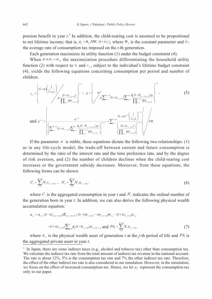
pension benefit in year t.2 In addition, the child-rearing cost is assumed to be proportional to net lifetime income; that is, ttgg ctNW , where is the constant parameter and tct the average rate of consumption tax imposed on the t-th generation.
Each generation maximizes its utility function (1) under the budget constraint (4).When , the maximization procedure differentiating the household utility
function (2) with respect to and , subject to the individual’s lifetime budget constraint (4), yields the following equations concerning consumption per period and number of children.
(5)
and
If the parameter is stable, these equations dictate the following two relationships: (1) as in any life-cycle model, the trade-off between current and future consumption is determined by the ratio of the interest rate and the time preference rate, and by the degree of risk aversion, and (2) the number of children declines when the child-rearing cost increases or the government subsidy decreases. Moreover, from these equations, the following forms can be shown:
Z
jjjttt cNC
M
jjjttt nNN (6)
where tC is the aggregated consumption in year t and tN indicates the ordinal number of the generation born in year t. In addition, we can also derive the following physical wealth accumulation equation:
jtjtjtjtjtjtjtjtjt ctcwwtwRtraa
j
g gjtjtgjt ntc , and Z
jjjttt aNPA (7)
where jta is the physical wealth asset of generation t at the j-th period of life and tPA is the aggregated private asset in year t.2 In Japan, there are some indirect taxes (e.g., alcohol and tobacco tax) other than consumption tax. We calculate the indirect tax rate from the total amount of indirect tax revenue in the national account. The rate is about 12%. 5% is the consumption tax rate and 7% the other indirect tax rate. Therefore, the effect of the other indirect tax rate is also considered in our simulation. However, in the simulation, we focus on the effect of increased consumption tax. Hence, we let tct represent the consumption tax only in our paper.

Policy Research Institute, Ministry of Finance, Japan, Public Policy Review, Vol.9, No.4, September 2013 643
(2) Firm behavior
The input/output structure is represented by the Cobb–Douglas production function with constant return to scale. The firm decides the demand for physical capital and effective labor in order to maximize its profit with the given factor prices of wage and rent, which are determined in the perfect competitive markets.
tett LAKY Q
j jtjt
te NeL (8)
ttt KIK (9)
where tY is the output, stands for capital income share, A is a scale parameter, tK is the physical capital stock, and teL is the effective labor.
We can derive two factor prices, the rate of return rt and the wage rate per unit of effective labor wt, by the first-order conditions for the firm’s maximum profit:
tettt LAKrR tett LAKw (10)
where is the depreciation of physical capital.
(3) The public pension
The pension sector grants a pension to the retiring generations while a pension premium is collected from the working generations.
tettt LwwP (11)
where tP stands for the aggregated pension premium.The aggregated pension benefits in year t is given by the product of the retirement-age
population, the replacement rate, and the average earnings of each generation during the working period .
Z
Qjjtjt
Z
Qjjtjtt NNqB (12)
where denotes the replacement rate and tB the aggregated pension benefit.We explicitly model the public pension system as a pay-as-you-go scheme. The budget
constraint of the pension sector can be shown as follows:
tt BspP (13)
where denotes the public subsidy to the pension scheme, financed by government expenditure tG .
Moreover, we assume that the public pension sector maintains a fixed replacement rate exogenously. As a result, in our model, the pension premium rate is endogenously determined in order to keep the budget constraint (13).

644 K Oguro, J Takahata / Public Policy Review
(4) The government
The government sector imposes four types of taxes: the wage tax, the consumption tax, the capital income tax, and the pension benefit tax.
ttttttttttettt BtpPARtrCHtcCtcLwtwT (14)
We keep all tax rates constant. The role of the government is to endogenously determine the rate of the public debt issue as a residual of government expenditure and revenue.
ttttt DrTGD (15)
where tG stands for government expenditure in year t, tT denotes tax revenue in year t, and tD denotes public debt in year t.
(5) Market equilibrium
Finally, in our closed-economy model, we require a financial market equilibrium, in which the aggregate value of assets equals the market value of capital stocks plus the value of outstanding government bonds:
ttt DKPA (16)
4. Data, Calibration, and Scenarios
In this section, we describe the outline of the data and the parameters of our model, and explain the scenarios of our simulation.
(1) Data and calibration
First, we present the values of the main parameters and exogenous variables of the model in Table 1. The parameter values for the households’ and firms’ behaviors are derived from Auerbach and Kotlikoff (1987) and various early OLG simulation studies in Japan.3 These parameters, such as the technological and preference parameters except the weight parameter
, are assumed to be constant.The exogenous variables, such as the macroeconomic, fiscal, and public pension variables,
are derived mainly from OECD (2007) and Whitehouse (2007).In addition, the child-bearing possibility parameter is derived from the “age-specific
fertility rate” data provided by the National Institute of Population and Social Security Research (2007), and the parameter values of the child-rearing cost and the government subsidy are derived from the special research report on the social cost of rearing children,
3 See Sadahiro and Shimasawa (2001, 2003), Uemura (2002), and Ihori et al. (2006).

Policy Research Institute, Ministry of Finance, Japan, Public Policy Review, Vol.9, No.4, September 2013 645
provided by the Director-General for Policies on a Cohesive Society, Cabinet Office, Japan (2005).
Second, by controlling the weight parameters during the years 1900–2007, we calibrate our demographic projection to fit the data’s trend in “Population by Age (generation born in 1900–2007),” provided by the Statistics Bureau, Ministry of Internal Affairs and Communications (MIAC), with the collaboration of other ministries and agencies in Japan.4 4 On the calibration with the demographic projection, we also control the weight parameter α in equa-tion (1) during the years 1900–2007. Concretely, we adapt the following operation. Let N*
t denote the population of the generation born in year t, provided by MIAC, and Nt, the population of the genera-tion born in year t in equation (6). The parameter αt in the utility of the generation born in year t in-creases (decreases), if Nt+Δ < N*
t+Δ ( Nt+Δ> N*t +Δ, e.g., Δ = 25). In addition, the parameter αt is fixed after
year 2007.
Table 1. Parameter values of the model
* This parameter is fixed after year 2007.
PARAMETER VALUE Utility function Time preference rate 0.01 Intertemporal elasticity of substitution /1 2.0
Weight parameter between number of children and consumption
0.84*
Production function Technology progress 0.002 Capital share in production 0.3 Physical capital depreciation 0.05 Tax policy parameters Wage tax tw 20.0% Capital tax tr 20.0% Consumption tax tc 5.0% Pension benefit tax tp 10.0% Pension policy parameters National subsidy to pension sp 25.0% Replacement ratio 50.0% Other parameters
0 to 5 0.78% 6 to 10 0.46% 11 to 15 0.55%
Child-rearing cost to net lifetime income
16 to 20 0.58%
1 to 5 3.0% 6 to 10 7.4% 11 to 15 7.0%
Childbearing possibility
16 to 20 2.6%
Government subsidy to child-rearing cost 0.1 Age-wage profile
0 1 2
88.3 7.08
-0.146 Age limit for childbearing M 40 Age of retirement Q 65 Average life expectancy Z 85
g
jp
g=
j=

646 K Oguro, J Takahata / Public Policy Review
Fig. 1 reports the actual and computed values of demographic projections. Note the close correspondence between the actual and calculated values.
In addition, since the model is simulated over 500 periods from 2007, the base year of our simulation, we ensure a sufficiently long period for a steady state to be achieved. In the simulation, we also keep the outstanding government debt to GDP at the same level after 2035, by controlling consumption tax. Table 2 reports the actual values of some key variables in 2007 and the computed values in the model. Further, it is observed that the actual values closely correspond to the calculated values.
Fig. 1. Demographic projection of each generation
OFFICIAL MODEL
National Income (% of GDP) Private consumption 74.1% 82.3% Government purchases of goods and services 21.0% 24.2%
Saving rate 3.1% 5.9% Government Indicators Pension premium to wage 14.9% 14.9% Gross public debt (% of GDP) 170.6% 172.2% Primary balance (% of GDP) -2.4% -4.3% Tax revenues (% of GDP) 18.4% 19.8% Other Indicators Capital output ratio 2.9 4.4 Interest rate 1.7% 2.6%
Table 2. Year 2007 of the baseline scenario
Source: OECD Economic Outlook No. 84, 2008, and “Annual Report on National Accounts,” the Japanese SNA statistics (Cabinet Office).

Policy Research Institute, Ministry of Finance, Japan, Public Policy Review, Vol.9, No.4, September 2013 647
(2) Scenarios
Next, we explain the simulation scenarios utilized in this paper. First of all, on August 10, 2012, in a plenary session of the House of Councillors, a comprehensive social security and tax reform bill (including a consumption tax increase) passed the three (Democratic Liberal, Liberal Democratic, and New Komeito) parties by a majority vote. As a result, the chance that the consumption tax will be raised to 8% in April 2014, and to 10% in October 2015, increased considerably. However, paragraph 3 of supplementary Article 18 of that law suggests that necessary measures to suspend enforcement are flexibly provided for, so future economic trends may determine whether or not the consumption tax is actually raised to 10%.
On the other hand, according to the Mid- to Long-term Economic Outlook (a conservative scenario) announced by the Cabinet office in August 2012, even if the consumption tax is raised to 10% by 2015, the fiscal balance (against GDP) is still forecast to be approximately 3% in the red. This implies that, because each 1% elevation of the consumption tax produces approximately 2.5 trillion yen in revenue, the consumption tax would need to be raised to 16% to achieve equilibrium with the Primary Balance by 2020. For this reason, the International Monetary Fund (IMF) indicates that Japan should reduce its growing sovereign debt, and gradually increase its consumption tax from 5% to 15% (June 17, 2011, Reuters).
We have considered 9 scenarios. Scenario 1 presents the basic case, calling for the consumption tax to remain at 5%, with neither expansion of child benefits nor cuts to pension benefits. Scenarios 2 to 5 assume 100% increase in child benefit after 2015. Then, the additional financial resource in Scenario 2 is covered by the increase in consumption tax, in Scenario 3 by the increase in wage tax, in Scenario 4 by the increase in capital income tax, and in Scenario 5 by the increase in government bond revenue. On the other hand, Scenarios 6 and 7 are those of the public pension reform. Scenario 6 assumes 50% reduction of the aggregated pension premium by increasing the consumption tax after 2015. Scenario 7 assumes 10% reduction of the public pension benefit and 100% increase in child benefit after 2015. Finally, Scenarios 8 and 9 are those of the accelerated fiscal reform. Scenario 8 assumes no expansion of child benefits but an increase in consumption tax to 15% (consumption tax reform) from 2015. Scenario 9 is the policy mix of Scenario 2 (permanent expansion) and Scenario 8.
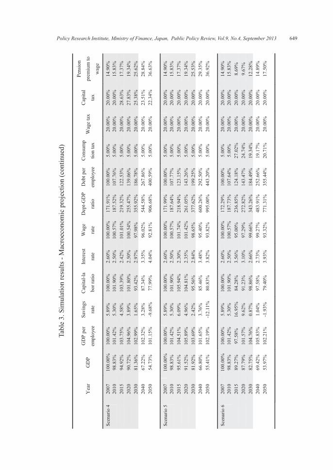
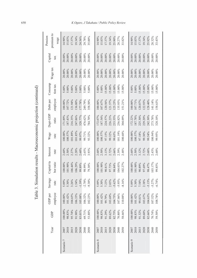
5. Simulation Results
This paper examines simulation results based on provisions in the 3rd and 4th sections. These simulation results are noted in Table 3 and Figs. 2 through 6. Table 3 shows macroeconomic trends, Fig. 2 depicts population transitions in future generations, Fig. 3 shows aging rate trends, Fig. 4 presents trends in total fertility rate (TFR), Fig. 5 lays out the public debt balance per employee, and Fig. 6 demonstrates each generation’s utility. We examine each of the above results in greater detail below.

648 K Oguro, J Takahata / Public Policy Review
Y
ear
GD
P G
DP
per
empl
oyee
Savi
ngs
rate
C
apita
l-la
bor r
atio
Inte
rest
rate
W
age
rate
D
ebt-G
D
P ra
tio
Deb
t per
empl
oyee
C
onsu
mp
tion
tax
Wag
e ta
xC
apita
l
tax
Pens
ion
prem
ium
to
wag
e
Scen
ario
1
2007
100.
00%
10
0.00
%5.
89%
100.
00%
2.60
%10
0.00
%17
1.80
%10
0.00
%5.
00%
20.0
0%20
.00%
14.9
0%
2010
98.8
3%
101.
42%
5.30
%10
1.90
%2.
50%
100.
57%
187.
35%
107.
73%
5.00
%20
.00%
20.0
0%15
.83%
20
1595
.29%
10
4.16
%5.
44%
104.
77%
2.35
%10
1.41
%21
7.95
%12
2.33
%5.
00%
20.0
0%20
.00%
17.3
7%
2020
91.4
5%
105.
81%
3.95
%10
4.57
%2.
36%
101.
35%
251.
98%
138.
48%
5.00
%20
.00%
20.0
0%19
.34%
20
3082
.29%
10
4.17
%0.
95%
97.0
3%2.
76%
99.1
0%34
6.93
%18
5.99
%5.
00%
20.0
0%20
.00%
25.4
4%
2040
68.1
5%
103.
95%
2.22
%91
.86%
3.06
%97
.48%
521.
09%
266.
57%
5.00
%20
.00%
20.0
0%28
.69%
20
5053
.83%
10
2.00
%-1
0.17
%78
.92%
3.97
%93
.14%
879.
92%
399.
80%
5.00
%20
.00%
20.0
0%37
.41%
Scen
ario
2
2007
100.
00%
10
0.00
%5.
89%
100.
00%
2.60
%10
0.00
%17
2.03
%10
0.00
%5.
00%
20.0
0%20
.00%
14.9
0%
2010
98.8
3%
101.
42%
5.30
%10
1.90
%2.
50%
100.
57%
187.
66%
107.
76%
5.00
%20
.00%
20.0
0%15
.83%
20
1594
.68%
10
3.49
%6.
66%
102.
53%
2.47
%10
0.75
%22
0.31
%12
2.68
%7.
39%
20.0
0%20
.00%
17.3
7%
2020
91.1
4%
105.
45%
4.72
%10
3.38
%2.
42%
101.
00%
255.
00%
139.
34%
7.24
%20
.00%
20.0
0%19
.34%
20
3082
.20%
10
4.06
%1.
27%
96.6
8%2.
78%
98.9
9%35
0.23
%18
5.47
%6.
96%
20.0
0%20
.00%
25.5
6%
2040
68.1
9%
103.
78%
2.64
%91
.56%
3.08
%97
.39%
527.
05%
262.
69%
6.70
%20
.00%
20.0
0%28
.82%
20
5054
.88%
10
1.30
%-8
.65%
78.4
4%4.
00%
92.9
7%87
5.87
%38
7.63
%6.
28%
20.0
0%20
.00%
36.8
5%
Sc
enar
io 3
20
0710
0.00
%
100.
00%
5.89
%10
0.00
%2.
60%
100.
00%
172.
02%
100.
00%
5.00
%20
.00%
20.0
0%14
.90%
20
1098
.83%
10
1.42
%5.
30%
101.
90%
2.50
%10
0.57
%18
7.68
%10
7.78
%5.
00%
20.0
0%20
.00%
15.8
3%
2015
95.6
2%
104.
52%
4.75
%10
5.98
%2.
29%
101.
76%
217.
60%
122.
38%
5.00
%22
.41%
20.0
0%17
.37%
20
2091
.55%
10
5.93
%3.
53%
104.
95%
2.34
%10
1.46
%25
2.18
%13
8.42
%5.
00%
22.4
6%20
.00%
19.3
4%
2030
82.1
2%
103.
95%
0.90
%96
.37%
2.80
%98
.90%
348.
75%
184.
45%
5.00
%22
.50%
20.0
0%25
.46%
20
4067
.92%
10
3.36
%2.
61%
90.3
4%3.
16%
97.0
0%52
7.48
%26
1.44
%5.
00%
22.4
5%20
.00%
28.7
8%
2050
54.7
9%
101.
02%
-8.7
3%77
.79%
4.06
%92
.74%
879.
55%
387.
28%
5.00
%22
.79%
20.0
0%36
.91%
Tabl
e 3.
Sim
ulat
ion
resu
lts -
Mac
roec
onom
ic p
roje
ctio
n
Dep
t-GD
P
ratio
Policy Research Institute, Ministry of Finance, Japan, Public Policy Review, Vol.9, No.4, September 2013 649
Y
ear
GD
P G
DP
per
empl
oyee
Savi
ngs
rate
C
apita
l-la
bor r
atio
Inte
rest
rate
W
age
rate
D
ebt-G
D
P ra
tio
Deb
t per
empl
oyee
Con
sum
p
tion
tax
Wag
e ta
xC
apita
l
tax
Pens
ion
prem
ium
to
wag
e Sc
enar
io 4
20
0710
0.00
%
100.
00%
5.89
%10
0.00
%2.
60%
100.
00%
171.
91%
100.
00%
5.00
%20
.00%
20.0
0%14
.90%
20
1098
.83%
10
1.42
%5.
30%
101.
90%
2.50
%10
0.57
%18
7.52
%10
7.76
%5.
00%
20.0
0%20
.00%
15.8
3%
2015
94.9
2%
103.
75%
4.58
%10
3.39
%2.
42%
101.
01%
219.
32%
122.
53%
5.00
%20
.00%
28.6
3%17
.37%
20
2090
.72%
10
4.96
%3.
89%
101.
80%
2.50
%10
0.54
%25
5.47
%13
9.06
%5.
00%
20.0
0%27
.83%
19.3
4%
2030
81.3
6%
102.
99%
1.65
%93
.42%
2.97
%97
.98%
355.
92%
186.
78%
5.00
%20
.00%
25.3
8%25
.62%
20
4067
.22%
10
2.32
%3.
28%
87.3
4%3.
35%
96.0
2%54
4.58
%26
7.86
%5.
00%
20.0
0%23
.51%
28.8
4%
2050
54.7
3%
101.
15%
-9.6
8%77
.99%
4.04
%92
.81%
906.
68%
400.
59%
5.00
%20
.00%
22.3
4%36
.63%
Scen
ario
5
2007
100.
00%
10
0.00
%5.
89%
100.
00%
2.60
%10
0.00
%17
1.99
%10
0.00
%5.
00%
20.0
0%20
.00%
14.9
0%
2010
98.8
3%
101.
42%
5.30
%10
1.90
%2.
50%
100.
57%
187.
64%
107.
77%
5.00
%20
.00%
20.0
0%15
.83%
20
1595
.61%
10
4.51
%6.
09%
105.
94%
2.30
%10
1.74
%21
8.94
%12
3.15
%5.
00%
20.0
0%20
.00%
17.3
7%
2020
91.5
2%
105.
89%
4.96
%10
4.81
%2.
35%
101.
42%
261.
05%
143.
26%
5.00
%20
.00%
20.0
0%19
.34%
20
3081
.92%
10
3.69
%2.
42%
95.5
6%2.
84%
98.6
5%37
7.62
%19
9.25
%5.
00%
20.0
0%20
.00%
25.5
3%
2040
66.8
0%
101.
65%
3.76
%85
.46%
3.48
%95
.40%
600.
26%
292.
50%
5.00
%20
.00%
20.0
0%29
.35%
20
5055
.41%
10
2.19
%-1
2.11
%80
.83%
3.82
%93
.82%
995.
00%
443.
20%
5.00
%20
.00%
20.0
0%36
.92%
Scen
ario
6
2007
100.
00%
10
0.00
%5.
89%
100.
00%
2.60
%10
0.00
%17
2.29
%10
0.00
%5.
00%
20.0
0%20
.00%
14.9
0%
2010
98.8
3%
101.
42%
5.30
%10
1.90
%2.
50%
100.
57%
187.
73%
107.
64%
5.00
%20
.00%
20.0
0%15
.83%
20
1589
.27%
97
.58%
16.9
5%84
.28%
3.56
%95
.00%
236.
85%
124.
18%
27.0
2%20
.00%
20.0
0%8.
69%
20
2087
.79%
10
1.57
%9.
62%
91.2
3%3.
10%
97.2
9%27
2.82
%14
3.47
%24
.74%
20.0
0%20
.00%
9.67
%
2030
82.7
5%
104.
76%
0.87
%98
.86%
2.66
%99
.66%
343.
26%
184.
49%
19.3
4%20
.00%
20.0
0%12
.28%
20
4069
.42%
10
5.83
%1.
04%
97.5
8%2.
73%
99.2
7%48
3.91
%25
2.66
%19
.17%
20.0
0%20
.00%
14.8
9%
2050
53.9
7%
102.
21%
-1.9
3%79
.40%
3.93
%93
.32%
771.
31%
355.
44%
20.7
1%20
.00%
20.0
0%17
.50%
Tabl
e 3.
Sim
ulat
ion
resu
lts -
Mac
roec
onom
ic p
roje
ctio
n (c
ontin
ued)
Dep
t-GD
P
ratio
650 K Oguro, J Takahata / Public Policy Review
Y
ear
GD
P G
DP
per
empl
oyee
Savi
ngs
rate
C
apita
l-la
bor r
atio
Inte
rest
rate
W
age
rate
D
ebt-G
D
P ra
tio
Deb
t per
empl
oyee
Con
sum
p
tion
tax
Wag
e ta
xC
apita
l
tax
Pens
ion
prem
ium
to
wag
e Sc
enar
io 7
20
0710
0.00
%
100.
00%
5.89
%10
0.00
%2.
60%
100.
00%
171.
89%
100.
00%
5.00
%20
.00%
20.0
0%14
.90%
20
1098
.83%
10
1.42
%5.
30%
101.
90%
2.50
%10
0.57
%18
7.43
%10
7.72
%5.
00%
20.0
0%20
.00%
15.8
3%
2015
95.7
4%
104.
65%
3.26
%10
6.44
%2.
27%
101.
89%
216.
35%
121.
94%
5.00
%20
.00%
20.0
0%17
.37%
20
2091
.90%
10
6.33
%1.
54%
106.
29%
2.28
%10
1.85
%24
7.86
%13
6.80
%5.
00%
20.0
0%20
.00%
19.3
4%
2030
83.0
1%
105.
08%
-1.3
9%99
.89%
2.60
%99
.97%
328.
77%
177.
78%
5.00
%20
.00%
20.0
0%24
.56%
20
4069
.71%
10
6.32
%-2
.70%
98.9
9%2.
65%
99.7
1%47
6.62
%24
9.79
%5.
00%
20.0
0%20
.00%
29.7
8%
2050
53.8
8%
102.
23%
-9.3
0%79
.30%
3.93
%93
.32%
784.
70%
358.
50%
5.00
%20
.00%
20.0
0%35
.00%
Scen
ario
8
2007
100.
00%
10
0.00
%5.
89%
100.
00%
2.60
%10
0.00
%17
2.07
%10
0.00
%5.
00%
20.0
0%20
.00%
14.9
0%
2010
98.8
3%
101.
42%
5.30
%10
1.90
%2.
50%
100.
57%
187.
54%
107.
67%
5.00
%20
.00%
20.0
0%15
.83%
20
1591
.29%
99
.79%
7.23
%90
.81%
3.13
%97
.15%
224.
57%
120.
56%
15.0
0%20
.00%
20.0
0%17
.37%
20
2089
.62%
10
3.69
%2.
03%
97.7
3%2.
72%
99.3
2%22
6.23
%12
1.57
%15
.00%
20.0
0%20
.00%
19.3
4%
2030
82.7
5%
104.
75%
-5.6
2%98
.84%
2.66
%99
.65%
233.
55%
125.
25%
15.0
0%20
.00%
20.0
0%25
.90%
20
4070
.80%
10
7.86
%-5
.95%
104.
03%
2.39
%10
1.19
%25
6.82
%13
5.93
%15
.00%
20.0
0%20
.00%
28.2
7%
2050
58.6
6%
110.
08%
-8.1
6%10
2.27
%2.
48%
100.
68%
304.
09%
151.
21%
15.0
0%20
.00%
20.0
0%33
.82%
Scen
ario
9
2007
100.
00%
10
0.00
%5.
89%
100.
00%
2.60
%10
0.00
%17
2.22
%10
0.00
%5.
00%
20.0
0%20
.00%
14.9
0%
2010
98.8
3%
101.
42%
5.30
%10
1.90
%2.
50%
100.
57%
187.
78%
107.
71%
5.00
%20
.00%
20.0
0%15
.83%
20
1591
.32%
99
.81%
7.54
%90
.89%
3.12
%97
.18%
225.
30%
120.
87%
15.0
0%20
.00%
20.0
0%17
.37%
20
2089
.60%
10
3.67
%2.
38%
97.6
9%2.
72%
99.3
0%22
9.20
%12
2.93
%15
.00%
20.0
0%20
.00%
19.3
4%
2030
82.6
6%
104.
63%
-5.1
5%98
.47%
2.68
%99
.54%
242.
30%
128.
40%
15.0
0%20
.00%
20.0
0%25
.92%
20
4070
.74%
10
7.52
%-5
.27%
103.
17%
2.43
%10
0.94
%27
3.78
%14
1.14
%15
.00%
20.0
0%20
.00%
28.3
2%
2050
59.5
0%
108.
74%
-6.7
4%99
.85%
2.60
%99
.95%
328.
10%
158.
63%
15.0
0%20
.00%
20.0
0%33
.43%
Tabl
e 3.
Sim
ulat
ion
resu
lts -
Mac
roec
onom
ic p
roje
ctio
n (c
ontin
ued)
Dep
t-GD
P
ratio

Policy Research Institute, Ministry of Finance, Japan, Public Policy Review, Vol.9, No.4, September 2013 651
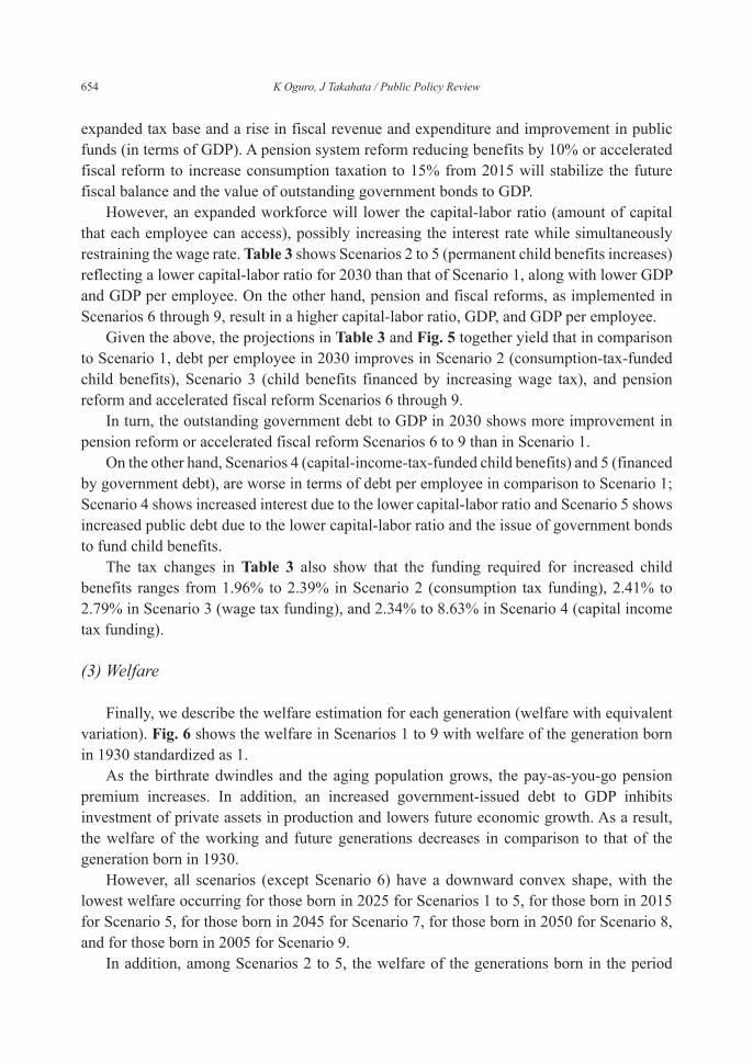
Fig. 2. Simulation results: demographic projection of future generations
Fig. 4. Simulation results: total fertility rate
Fig. 3. Simulation results: retired population ratio
652 K Oguro, J Takahata / Public Policy Review
(1) Demographic projection and macroeconomic variables
First, we describe the demographic projection. Fig. 2 shows the population projection of future generations born in the period 2000–2030. The projection in Scenario 1 closely corresponds to the official estimation provided by the National Institute of Population and Social Security Research (2006). In contrast to Scenario 1, Scenarios 2 to 5 (100% permanent child benefits increases) and 8 and 9 (accelerated fiscal reform and 100% permanent child benefits increase) depict a population increase in the generation born after 2015. On the other hand, Scenarios 6 (50% reduction of the aggregated pension premium by increasing consumption tax) and 7 (10% reduction of the public pension benefit and 100% permanent child benefits increase) show a population decrease. In Scenario 9 (accelerated fiscal reform
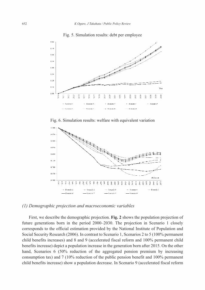
Fig. 5. Simulation results: debt per employee
Fig. 6. Simulation results: welfare with equivalent variation

Policy Research Institute, Ministry of Finance, Japan, Public Policy Review, Vol.9, No.4, September 2013 653
and 100% permanent child benefits increase), the population of the generation born in 2030 is the highest, increasing by 181,000.
The population under Scenario 5 (financed by government debt) shows an increase of 160,000; followed by the population under Scenario 3 (child benefits financed by increasing wage tax) with an increase of 158,000; the population under Scenario 2 (consumption-tax-funded child benefits) with an increase of 149,000; and, finally the population under Scenario 4 (capital-income-tax-funded child benefits) with an increase of 146,000. Scenario 8 (only accelerated fiscal reform) shows an increase of 32,000 while Scenario 6 (half of the pension premium covered by consumption tax) demonstrates a decrease of 19,000 and Scenario 7 (10% reduction of the public pension benefit and 100% permanent child benefits increase), shows a decrease of 11,000.
Fig. 4 shows the total fertility rate (TFR) from 1995 to 2030. The projections in Scenario 1 closely correspond to the official estimation provided by the National Institute of Population and Social Security Research (2006). Fig. 2 shows a TFR projection for all scenarios. For example, Scenario 9 shows the highest TFR with 1.51, followed by Scenario 5 with 1.48, and Scenario 3 with 1.47 in 2030.
Fig. 3 shows a projection of the retired population ratio from 2010 to 2050. The projection in Scenario 1 closely corresponds to the official estimation provided by the National Institute of Population and Social Security Research (2006). In comparison to Scenario 1, the 2030 retired population ratio in Scenarios 2 to 5, with permanent child benefit increases, decreases between 0.30% of a point and 0.32% of a point. Similarly, the ratio in Scenario 9 decreases by 0.43% of a point, not a highly significant difference. Further, the 2050 retired population ratio in Scenarios 2 to 5, with permanent child benefit increases, decreases between 1.4% of a point and 1.9% of a point, compared to the other scenarios. Regardless of the long-term improvements, in the short term, it seems unlikely that the retired population rate will decrease to any significant degree in response to child-rearing benefits.
Next, we simply explain the projection from a macroeconomic perspective. As our model employs a life-cycle hypothesis, the savings rate is highly influenced by the aging population. Looking at the transition of macroeconomic variables shown in Table 3, though some cases show a temporary rise, in 2030 all scenarios show a decrease in the savings rate (between -5.62% and 2.42%), compared to the 2007 rate of 5.89%. In particular, in comparison to Scenario 1, Scenarios 2 (child benefits expansion financed by consumption tax, and permanent child benefits increases), 4 (funded by capital income tax), and 5 (funded by government debt), show a rise in the savings rate in 2030. Further, although Scenarios 1 to 6 show a rise in the savings rate in 2040, all scenarios show a decrease in 2050. Finally, the factor price shows a stable transition in all scenarios, fluctuating between the interest rates of 2.27% (wage rate) and 4.04% (92.74% to 101.89%).
(2) Fiscal variables
In general, increased child benefits lead to more births, creating a greater workforce and
654 K Oguro, J Takahata / Public Policy Review
expanded tax base and a rise in fiscal revenue and expenditure and improvement in public funds (in terms of GDP). A pension system reform reducing benefits by 10% or accelerated fiscal reform to increase consumption taxation to 15% from 2015 will stabilize the future fiscal balance and the value of outstanding government bonds to GDP.
However, an expanded workforce will lower the capital-labor ratio (amount of capital that each employee can access), possibly increasing the interest rate while simultaneously restraining the wage rate. Table 3 shows Scenarios 2 to 5 (permanent child benefits increases) reflecting a lower capital-labor ratio for 2030 than that of Scenario 1, along with lower GDP and GDP per employee. On the other hand, pension and fiscal reforms, as implemented in Scenarios 6 through 9, result in a higher capital-labor ratio, GDP, and GDP per employee.
Given the above, the projections in Table 3 and Fig. 5 together yield that in comparison to Scenario 1, debt per employee in 2030 improves in Scenario 2 (consumption-tax-funded child benefits), Scenario 3 (child benefits financed by increasing wage tax), and pension reform and accelerated fiscal reform Scenarios 6 through 9.
In turn, the outstanding government debt to GDP in 2030 shows more improvement in pension reform or accelerated fiscal reform Scenarios 6 to 9 than in Scenario 1.
On the other hand, Scenarios 4 (capital-income-tax-funded child benefits) and 5 (financed by government debt), are worse in terms of debt per employee in comparison to Scenario 1; Scenario 4 shows increased interest due to the lower capital-labor ratio and Scenario 5 shows increased public debt due to the lower capital-labor ratio and the issue of government bonds to fund child benefits.
The tax changes in Table 3 also show that the funding required for increased child benefits ranges from 1.96% to 2.39% in Scenario 2 (consumption tax funding), 2.41% to 2.79% in Scenario 3 (wage tax funding), and 2.34% to 8.63% in Scenario 4 (capital income tax funding).
(3) Welfare
Finally, we describe the welfare estimation for each generation (welfare with equivalent variation). Fig. 6 shows the welfare in Scenarios 1 to 9 with welfare of the generation born in 1930 standardized as 1.
As the birthrate dwindles and the aging population grows, the pay-as-you-go pension premium increases. In addition, an increased government-issued debt to GDP inhibits investment of private assets in production and lowers future economic growth. As a result, the welfare of the working and future generations decreases in comparison to that of the generation born in 1930.
However, all scenarios (except Scenario 6) have a downward convex shape, with the lowest welfare occurring for those born in 2025 for Scenarios 1 to 5, for those born in 2015 for Scenario 5, for those born in 2045 for Scenario 7, for those born in 2050 for Scenario 8, and for those born in 2005 for Scenario 9.
In addition, among Scenarios 2 to 5, the welfare of the generations born in the period
Policy Research Institute, Ministry of Finance, Japan, Public Policy Review, Vol.9, No.4, September 2013 655
1955 to 1980 is lowest in Scenario 2 (child benefits expansion financed by consumption tax). As briefly explained in Section 2, this indicates that child benefits expansion funded by consumption tax results in an intergenerational income transfer from the retired to the younger generation.
On the other hand, the welfare for the generation born in 2050 is the highest in Scenario 5 (financed by government debt). The next highest figure is for Scenario 4 (capital-income-tax-funded child benefits), followed by Scenario 2 (consumption-tax-funded child benefits), and Scenario 3 (child benefits financed by increasing wage tax). Next is Scenario 6 (half of the pension premium covered by consumption tax), then Scenario 1 (current case), Scenario 9 (accelerated fiscal reform and 100% permanent child benefits increase), Scenario 8 (only accelerated fiscal reform), and Scenario 7 (10% reduction of the public pension benefit and 100% permanent child benefits increase) in that order.
Placing the highest importance on the welfare of future generations, Scenario 5 (financed by government debt) stands out as the most desirable option, but a closer look is necessary. Table 3 shows that Scenarios 1 through 7, without accelerated fiscal reform, public debt to GDP increases to over 300%. Therefore, from the standpoint of improving financial sustainability, it is likely that accelerated fiscal reform is unavoidable. In particular, in 2030, Scenarios 2 to 4 show public debt to GDP between 348% and 355% while in Scenario 5 it rises to approximately 377% (in 2050 as well). In the case when funding of child benefits cannot be financed by public debt, Scenario 4 (capital-income-tax-funded child benefits) becomes the better option.
6. Conclusion and Future Issues
In this paper, we presented an OLG model with multi-concurrent generations and endogenous fertility to analyze the effects of increased child benefits and reduced pension benefits on the welfare of the working and future generations. The following results were obtained through the analysis.
First, when child benefits and accelerated fiscal reform are combined, the most benefit can be gained in terms of the influence on demographics. When child benefits are not funded by accelerated fiscal reform, funding through issuing of government bonds, by wage� taxation, by consumption tax, and by capital income taxation, in that order, showed effectiveness.
In terms of the influence on future public debt, compared with figures projected in 2030 under the current situation, the options that have an effect are pension reform and accelerated fiscal reform; the option of higher consumption tax has a particularly strong effect.
Further, achieving either pension reform or accelerated fiscal reform together with either consumption tax or capital income tax shows improvement in terms of public debt per individual. This is because child benefits result in more people in future generations, and this larger population can shoulder the burden of public debt.
With regard to the influence in society from now on, in comparison with the generation

656 K Oguro, J Takahata / Public Policy Review
born in 2050, issuance of public bonds as funding for child benefits is most effective, while capital-income-tax-funded child benefits, then consumption-tax-funded child benefits, in that order, showed effect. It is important to note that compared to other scenarios, issuing public bonds raises the public debt; therefore, from the viewpoint of financial sustainability, accelerated fiscal reform will be necessary as it looks difficult to provide benefits to the generation born after 2050.
Two issues remain. First, if households focus on factors of quality or of human capital in terms of their budgets, it is possible that the results will differ. If household budgets consider, in addition to the number of children, whether the aspect of quality is able to delivery utility, the macroeconomics of child benefit may vary. For example, if child expenses are high and education expenditure is also assessed as high, a subsidy may be provided. In that case, because costs associated with children are lessened, the number of children born may increase, possibly resulting in lower quality of life for the children who then may have lower productivity. In this way, if quality or human capital are taken into consideration, implications regarding the options may differ.
Second, child support that considers factors other than cost has not been considered. Whether the environment is supportive of raising children is naturally an influencing factor on whether the household decided whether or not to have children. While this paper dealt only with models that looked at the cost of raising children, other factors including availability of day care and other services certainly influence the decision. When making policy for child benefit, besides financial factors, it is essential to include in the proposal overall infrastructure conditions of the society.
In general, simulation analysis brings out multiple effects depending on the policy. To observe how macroeconomics change in quantitative form the general equilibrium analysis used here is especially useful. However, as mentioned above, several factors for testing remain and further research on this model is required.
References
・ Abío, G., G. Mahieu, and C. Patxot (2004), “On the Optimality of PAYG Pension Systems in an Endogenous Fertility Setting,” Journal of Pension Economics and Finance 3, pp35-62.
・ Atkinson, A. B. and Stiglitz, J. E. (1972), “The Structure of Indirect Taxation and Economic Efficiency,” Jounal of Public Economics, 1, pp. 97-119.
・ Atkinson, A. B. and Stiglitz, J. E. (1976), “The Design of Tax Structure: Direct Versus Indirect Taxation,” Journal of Public Economics, 6(1-2), pp. 55-75.
・ Barro, R. and G. S. Becker (1989), “Fertility Choice in a Model of Economic Growth,” Econometrica 57, pp481-501.
・ Becker, G. S. (1960), “An economic analysis of fertility. In: Demographic and economic change in developed countries,” National Bureau of Economic Research Conference Series 11, pp. 209–231.

Policy Research Institute, Ministry of Finance, Japan, Public Policy Review, Vol.9, No.4, September 2013 657
・ Becker, G. S. and R. Barro (1988), “A Reformulation of the Economic Theory of Fertility,” Quarterly Journal of Economics 103, pp1-25.
・ Becker, G. S. and H. G. Lewis (1973), “On the Interaction between the Quantity and Quality of Children,”Journal of Political Economy 81, ppS279-S288.
・ Bental, B. (1989), “The Old Age Security Hypothesis and Optimal Population Growth,” Journal of Population Economics 1, pp285-301.
・ Chamley, C. (1986), “Optimal Taxation of Capital Income in General Equilibrium with Infinite Lives,” Econometrica, 54(3), pp. 607-22.
・ Cigno, A. (1983), “On Optimal Family Allowances,” Oxford Economic Papers 35, pp13-22.
・ Conesa, J. C., Kitao, S. and Krueger, D. (2007), “Taxing Capital? Not a Bad Idea After All!” NBER Working Paper 12880.
・ Cremer, H., and Gahvari, F. (1995), “Uncertainty, Optimal Taxation and the Direct Versus Indirect Tax Controversy,” Economic Journal, 105, pp. 1165-1179.
・ Cremer, H., F. Gahvari, and P. Pestieau (2006), “Pensions with Endogenous and Stochastic Fertility,” Journal of Public Economics 90, pp2303-2321.
・ Cremer, H., F. Gahvari, and P. Pestieau (2008), “Pensions with Heterogenous Individuals and Endogenous Fertility,” Journal of Population Economics 21, pp961-981.
・ Deardorff, A. V. (1976), “The Optimum Growth Rate for Population: Comment,” International Economic Review 17, pp510-515.
・ Diamond, P.A. (1965), “National Debt in a Neoclassical Growth Model,” American Economic Review 55(5), pp. 1126–1150.
・ Eckstein, Z. and K. Wolpin (1985), “Endogenous Fertility and Optimal Population Size,” Journal of Public Economics 87, pp233-251.
・ Fenge, R. and V. Meier (2009), “ Are family allowances and fertility-related pensions perfect substitutes?," International Tax and Public Finance 16, pp137-63.
・ Golosov, M., L. Jones, and M. Tertilt (2007), “Efficiency with Endogenous Population Growth,” Econometrica 75, pp1039-1071.
・ Hatta, T., and Oguchi, Y. (1999), The Theory of Public Pension Reform: Transform to Funding System. Nikkei Publishing, Inc. [in Japanese].
・ Hubbard, R. G., and Judd, K. L. (1986), “Liquidity Constraints, Fiscal Policy, and Consumption,” Brookings Papers on Economic Activity. 1, pp. 1-59.
・ Ihori, T., Kato, R., Kawade, M. and Bessho, S. (2006). “Public debt and economic growth in an aging Japan,” K. Kaizuka and Ann O. Krueger, eds., Tackling Japan's Fiscal Challenges: Strategies to Cope with High Public Debt and Population Aging. [in Japanese]
・ Judd, K. L. (1985), “Redistributive Taxation in a Simple Perfect Foresight Model,” Journal of Public Economics, 28(1), pp. 59-83.
・ Michel Ph. and P. Pestieau (1993), “Population Growth and Optimality,” Journal of Population Economics 6, pp353-362.
・ Michel, Ph. and B. Wigniolle (2007), “On Efficient Child Making,” Economic Theory 31,

658 K Oguro, J Takahata / Public Policy Review
pp307-326.・ National Institute of Population and Social Security Research. Population Statistics of
Japan, 2007. [in Japanese]・ ________. Population Projections for Japan: 2006-2055, 2006.・ Nerlove, M., A. Razin and E. Sadka (1986), “Some Welfare Theoretic Implications of
Endogenous Fertility,” International Economic Review 27, pp3-31.・ Nishimura, K. and Zhang, J. (1992), “Pay-as-you-go public pensions with endogenous
fertility,” Journal of Public Economics 48, pp. 239–258. ・ Nishimura, K. and J. Zhang (1995), “Sustainable Plans of Social Security with Endogenous
Fertility,” Oxford Economic Papers 47, pp182-194.・ OECD. Tax Database, Paris, 2007.・ Oguro, K., Takahata, J. and Shimasawa, M. (2009), “Child Benefit and Fiscal Burden:
OLG model with Endogenous Fertility,” IPSS Discussion Paper Series 2009-E01.・ Sadahiro, A., and M. Shimasawa (2001). “Fiscal Sustainability and the Primary Surplus: A
Simulation Analysis with OLG Model,” JCER Economic Journal 43. pp. 117–132. [in Japanese]
・ ________ and ________ (2003). “The computable overlapping generations model with an endogenous growth mechanism,” Economic Modeling 20(1), pp. 1–24.
・ Saez, E. (2002), “The Desirability of Commodity Taxation under Non-Linear Income Taxation and Heterogeneous Tastes,” Journal of Public Economics, 83(2), pp. 217-30.
・ Samuelson, P. A. (1958), “An Exact Consumption-Loan Model of Interest with or without the Social Contrivance of Money,” Journal of Political Economy 66, pp467-482.
・ Samuelson, P. A. (1975), “The Optimum Growth Rate for Population,” International Economic Review 16, pp531-538.
・ Samuelson, P. A. (1976), “The Optimum Growth Rate for Population: Agreement and Evaluations,” International Economic Review 17, pp516-525.
・ Uemura, T. (2002). “Lifecycle General Equilibrium Analysis on Social Security,” Keizaironshu 28(1). [in Japanese]
・ van Groezen, B., T. Leers, and L. Mejidam (2003), “Social security and endogenous fertility: pensions and child allowances as Siamese twins,” Journal of Public Economics 87, pp233-251.
・ Weinzierl, M. (2007), “The Surprising Power of Age-Dependent Taxes,” Unpublished. http://www.econ.yale.edu/seminars/jr-fac/jf08/Weinzierl_JMP.pdff
・ Whitehouse, Edward. Pensions Panorama: Retirement-Income Systems in 53 Countries, The World Bank, 2007.
・ Willis, R. J. (1973), “A New Approach to the Economic Theory of Fertility Behavior,” Journal of Political Economy 81, ppS14-S64.
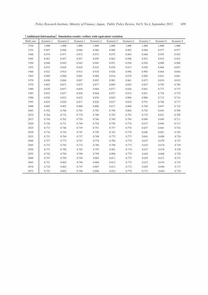
Policy Research Institute, Ministry of Finance, Japan, Public Policy Review, Vol.9, No.4, September 2013 659
Additional Information Simulation results: welfare with equivalent variation Birth year Scenario 1 Scenario 2 Scenario 3 Scenario 4 Scenario 5 Scenario 6 Scenario 7 Scenario 8 Scenario 9
1930 1.000 1.000 1.000 1.000 1.000 1.000 1.000 1.000 1.000 1935 0.987 0.986 0.986 0.986 0.988 0.983 0.984 0.977 0.977 1940 0.974 0.971 0.972 0.973 0.975 0.965 0.968 0.955 0.955 1945 0.961 0.957 0.957 0.959 0.963 0.948 0.952 0.932 0.932 1950 0.948 0.943 0.943 0.945 0.951 0.930 0.936 0.909 0.909 1955 0.935 0.928 0.929 0.932 0.938 0.913 0.920 0.886 0.887 1960 0.922 0.914 0.915 0.918 0.926 0.896 0.905 0.864 0.864 1965 0.909 0.900 0.901 0.904 0.914 0.878 0.889 0.841 0.841 1970 0.896 0.886 0.887 0.891 0.901 0.861 0.873 0.818 0.819 1975 0.883 0.871 0.872 0.877 0.889 0.843 0.857 0.795 0.796 1980 0.870 0.857 0.858 0.864 0.877 0.826 0.841 0.773 0.773 1985 0.852 0.837 0.838 0.844 0.857 0.812 0.821 0.738 0.739 1990 0.838 0.823 0.822 0.830 0.842 0.806 0.806 0.715 0.716 1995 0.824 0.820 0.817 0.826 0.837 0.810 0.791 0.706 0.717 2000 0.803 0.803 0.800 0.808 0.817 0.808 0.768 0.697 0.710 2005 0.782 0.788 0.783 0.792 0.798 0.802 0.743 0.692 0.708 2010 0.764 0.776 0.770 0.780 0.783 0.793 0.719 0.691 0.709 2015 0.744 0.762 0.756 0.766 0.769 0.784 0.696 0.689 0.711 2020 0.726 0.751 0.744 0.754 0.758 0.776 0.675 0.686 0.713 2025 0.715 0.746 0.739 0.751 0.757 0.770 0.657 0.683 0.716 2030 0.716 0.754 0.747 0.758 0.765 0.770 0.646 0.681 0.720
2035 0.721 0.764 0.757 0.768 0.775 0.773 0.641 0.680 0.724 2040 0.727 0.773 0.767 0.778 0.786 0.774 0.637 0.678 0.727 2045 0.733 0.782 0.776 0.786 0.794 0.775 0.635 0.674 0.729 2050 0.737 0.788 0.783 0.793 0.801 0.774 0.637 0.670 0.728 2055 0.742 0.794 0.789 0.799 0.806 0.774 0.643 0.668 0.728 2060 0.747 0.799 0.794 0.803 0.811 0.773 0.655 0.671 0.731 2065 0.751 0.802 0.796 0.806 0.813 0.773 0.672 0.676 0.735 2070 0.754 0.802 0.797 0.807 0.813 0.772 0.692 0.680 0.737 2075 0.755 0.802 0.796 0.806 0.812 0.770 0.713 0.684 0.739

660 K Oguro, J Takahata / Public Policy Review