Chi-Square ( 2) Test of Association Chi-Square Test of ... · PDF fileChi-Square ( 2) Test of...
12
Chi-Square ( 2 ) Test of Association Chi-Square Test of Association or Chi-Square Test of Contingency Tables: Analysis of Association Between Two Nominal or Categorical Variables With the goodness-of-fit test one is interested in determining whether a given distribution of data follows an expected pattern. For the test of association, however, one is interested in learning whether two (or more) categorical variables are related. Typically one will find two categorical variables depicted in a contingency table (a cross-tabulation of the frequencies for various combinations of the variables). Note that contingency tables are referred to as 2-by-3, 3-by-3, etc. where the numerals are determined by the number of rows (R) and columns (C) in the table. If, for example, there is a table with two rows and two columns, the table is a R x C or 2 x 2 (2-by-2) table. 1. Example with Tenure Status and Policy Support At issue in the following research question is whether the policy of allowing college faculty to take-on outside consultation for a fee is supported uniformly between tenured and untenured faculty. The data are as follows (example taken from D. E. Hinkle et al., 1979, Applied statistics for he behavioral sciences, Rand McNally): Table 1 Policy Support by Tenure Status Support Policy Do not Support Policy Tenured 88 17 Nontenured 84 11 Total = 200. 2. Hypotheses The null hypothesis states that there is no relationship between the two variables, i.e., that support for the consulting policy is independent of the tenure status of the faculty; or, that there is no difference between tenured and nontenured faculty regarding their support of the consulting policy. H 0 : distribution tenured = distribution nontenured (or the distributions are equal) or H 0 : variable A (policy support) is independent of variable B (tenure status) and the alternative hypothesis is: H 1 : some difference in the distributions or H 1 : variables A and B are associated, not independent
Transcript of Chi-Square ( 2) Test of Association Chi-Square Test of ... · PDF fileChi-Square ( 2) Test of...
Chi-Square (2) Test of Association
Chi-Square Test of Association or Chi-Square Test of Contingency Tables:
Analysis of Association Between Two Nominal or Categorical Variables
With the goodness-of-fit test one is interested in determining whether a given distribution of data follows an expected
pattern. For the test of association, however, one is interested in learning whether two (or more) categorical variables are
related. Typically one will find two categorical variables depicted in a contingency table (a cross-tabulation of the
frequencies for various combinations of the variables). Note that contingency tables are referred to as 2-by-3, 3-by-3, etc.
where the numerals are determined by the number of rows (R) and columns (C) in the table. If, for example, there is a
table with two rows and two columns, the table is a R x C or 2 x 2 (2-by-2) table.
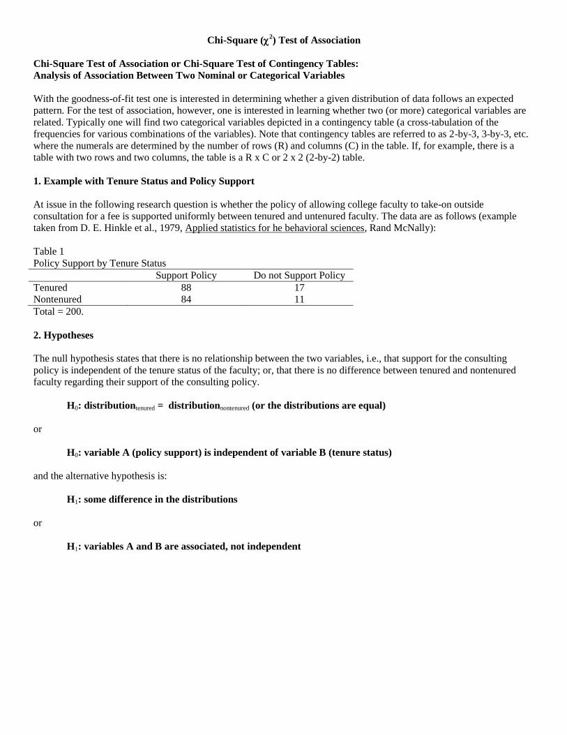
1. Example with Tenure Status and Policy Support
At issue in the following research question is whether the policy of allowing college faculty to take-on outside
consultation for a fee is supported uniformly between tenured and untenured faculty. The data are as follows (example
taken from D. E. Hinkle et al., 1979, Applied statistics for he behavioral sciences, Rand McNally):
Table 1
Policy Support by Tenure Status
Support Policy Do not Support Policy
Tenured 88 17
Nontenured 84 11
Total = 200.
2. Hypotheses
The null hypothesis states that there is no relationship between the two variables, i.e., that support for the consulting
policy is independent of the tenure status of the faculty; or, that there is no difference between tenured and nontenured
faculty regarding their support of the consulting policy.
H0: distributiontenured = distributionnontenured (or the distributions are equal)
or
H0: variable A (policy support) is independent of variable B (tenure status)
and the alternative hypothesis is:
H1: some difference in the distributions
or
H1: variables A and B are associated, not independent
2
Version: 10/14/2013
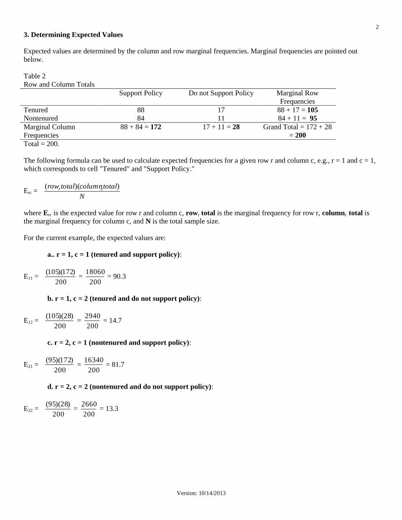
3. Determining Expected Values
Expected values are determined by the column and row marginal frequencies. Marginal frequencies are pointed out
below.
Table 2
Row and Column Totals
Support Policy Do not Support Policy Marginal Row
Frequencies
Tenured 88 17 88 + 17 = 105
Nontenured 84 11 84 + 11 = 95
Marginal Column
Frequencies
88 + 84 = 172 17 + 11 = 28 Grand Total = 172 + 28
= 200
Total = 200.
The following formula can be used to calculate expected frequencies for a given row r and column c, e.g., r = 1 and c = 1,
which corresponds to cell "Tenured" and "Support Policy."
Erc = N
totalcolumntotalrow cr ))((
where Erc is the expected value for row r and column c, rowr total is the marginal frequency for row r, columnc total is
the marginal frequency for column c, and N is the total sample size.
For the current example, the expected values are:
a.. r = 1, c = 1 (tenured and support policy):
E11 = 200
)172)(105( =
200
18060 = 90.3
b. r = 1, c = 2 (tenured and do not support policy):
E12 = 200
)28)(105( =
200
2940 = 14.7
c. r = 2, c = 1 (nontenured and support policy):
E21 = 200
)172)(95( =
200
16340 = 81.7
d. r = 2, c = 2 (nontenured and do not support policy):
E22 = 200
)28)(95( =
200
2660 = 13.3
3
Version: 10/14/2013
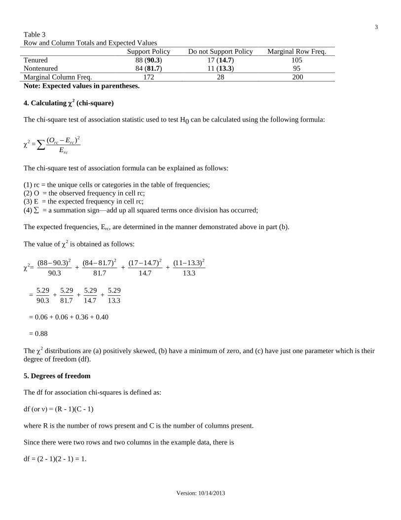
Table 3
Row and Column Totals and Expected Values
Support Policy Do not Support Policy Marginal Row Freq.
Tenured 88 (90.3) 17 (14.7) 105
Nontenured 84 (81.7) 11 (13.3) 95
Marginal Column Freq. 172 28 200
Note: Expected values in parentheses.
4. Calculating 2 (chi-square)
The chi-square test of association statistic used to test H0 can be calculated using the following formula:
2 =
rc
rcrc
E
EO 2)(
The chi-square test of association formula can be explained as follows:
(1) rc = the unique cells or categories in the table of frequencies;
(2) O = the observed frequency in cell rc;
(3) E = the expected frequency in cell rc;
(4) = a summation sign—add up all squared terms once division has occurred;
The expected frequencies, Erc, are determined in the manner demonstrated above in part (b).
The value of 2 is obtained as follows:
2=
3.90
)3.9088( 2 +
7.81
)7.8184( 2 +
7.14
)7.1417( 2 +
3.13
)3.1311( 2
= 3.90
29.5 +
7.81
29.5 +
7.14
29.5 +
3.13
29.5
= 0.06 + 0.06 + 0.36 + 0.40
= 0.88
The 2 distributions are (a) positively skewed, (b) have a minimum of zero, and (c) have just one parameter which is their
degree of freedom (df).
5. Degrees of freedom
The df for association chi-squares is defined as:
df (or ν) = (R - 1)(C - 1)
where R is the number of rows present and C is the number of columns present.
Since there were two rows and two columns in the example data, there is
df = (2 - 1)(2 - 1) = 1.
4
Version: 10/14/2013
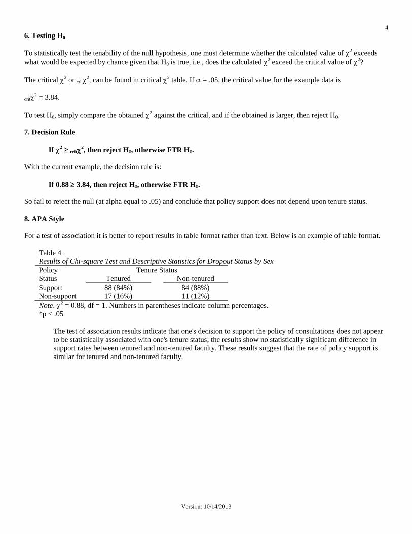
6. Testing H0
To statistically test the tenability of the null hypothesis, one must determine whether the calculated value of 2 exceeds
what would be expected by chance given that H0 is true, i.e., does the calculated 2 exceed the critical value of
2?
The critical 2 or crit
2, can be found in critical
2 table. If = .05, the critical value for the example data is
crit2 = 3.84.
To test H0, simply compare the obtained 2 against the critical, and if the obtained is larger, then reject H0.
7. Decision Rule
If 2 crit
2, then reject H0, otherwise FTR H0.
With the current example, the decision rule is:
If 0.88 3.84, then reject H0, otherwise FTR H0.
So fail to reject the null (at alpha equal to .05) and conclude that policy support does not depend upon tenure status.
8. APA Style
For a test of association it is better to report results in table format rather than text. Below is an example of table format.
Table 4
Results of Chi-square Test and Descriptive Statistics for Dropout Status by Sex
Policy Tenure Status
Status Tenured Non-tenured
Support 88 (84%) 84 (88%)
Non-support 17 (16%) 11 (12%)
Note. 2 = 0.88, df = 1. Numbers in parentheses indicate column percentages.
*p < .05
The test of association results indicate that one's decision to support the policy of consultations does not appear
to be statistically associated with one's tenure status; the results show no statistically significant difference in
support rates between tenured and non-tenured faculty. These results suggest that the rate of policy support is
similar for tenured and non-tenured faculty.

5
Version: 10/14/2013
9. Example with Abortion Support by Party Identification
Table 5 shows Gallup’s (May 23, 2011) reported split between pro-life and pro-choice among political party identification
lines.
Table 5
Abortion Support by Party Identification
Abortion Stance Republican Independent Democrat
Pro-life 13 8 5
Pro-choice 5 9 13
N = 53
Do the data show evidence of a difference in support among the three political groups?
10. Hypotheses
The null hypothesis states that there is no relationship between the two variables or no difference in support choices
among the three groups.
H0: Abortion Stance is independent of Political Party, or
H0: Abortion Stance Distribution is the same across Political Parties
H1: Abortion Stance and Political Party are associated, or
H1: Abortion Stance Distribution varies across Political Parties
11. Determining Expected Values
Expected values are determined by the column and row marginal frequencies. Marginal frequencies are pointed out
below.
Table 6
Abortion Support by Party Identification: Row and Column Totals
Abortion Stance Republican Independent Democrat Row Totals
Pro-life 13 8 5 26
Pro-choice 5 9 13 27
Column Totals 18 17 18
Expected values entered in parentheses below. Recall that expected values are determined by this formula:
Expected Value = (Row Total × Column Total) / Overall Total
Example for Independent, Pro-life cell: (17 × 26) / 53 = 442 / 53 = 8.34
Table 7
Abortion Support by Party Identification: Row and Column Totals and Expected Values
Abortion Stance Republican Independent Democrat Row Totals
Pro-life 13 (8.83) 8 (8.34) 5 (8.83) 26
Pro-choice 5 (9.17) 9 (8.66) 13 (9.17) 27
Column Totals 18 17 18 N=53
Note: Expected values in parentheses.

6
Version: 10/14/2013
12. Calculating 2 (chi-square)
The chi-square test of association statistic used to test H0 can be calculated using the following formula:
2 =
rc
rcrc
E
EO 2)(
The chi-square test of association formula can be explained as follows:
(1) rc = the unique cells or categories in the table of frequencies;
(2) O = the observed frequency in cell rc;
(3) E = the expected frequency in cell rc;
(4) = a summation sign—add up all squared terms once division has occurred;
The expected frequencies, Erc, are determined in the manner demonstrated above.
The value of 2 is obtained as follows:
Table 9
Abortion Support by Party Identification: Row and Column Totals and Expected Values
Abortion Stance Republican Independent Democrat Row Totals
Pro-life 13 (8.83) 8 (8.34) 5 (8.83) 26
Pro-choice 5 (9.17) 9 (8.66) 13 (9.17) 27
Column Totals 18 17 18 N=53
Note: Expected values in parentheses.
13. Degrees of freedom
The df for association chi-squares is defined as:
df (or ν) = (R - 1)(C - 1)
Since there were two rows and three columns in the example data, there is
df = (2 - 1)(3 - 1) = 2.
7
Version: 10/14/2013
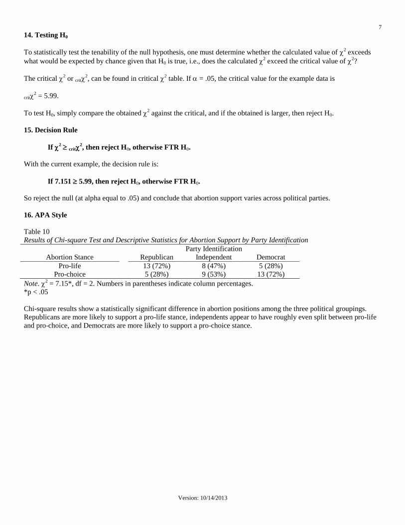
14. Testing H0
To statistically test the tenability of the null hypothesis, one must determine whether the calculated value of 2 exceeds
what would be expected by chance given that H0 is true, i.e., does the calculated 2 exceed the critical value of
2?
The critical 2 or crit
2, can be found in critical
2 table. If = .05, the critical value for the example data is
crit2 = 5.99.
To test H0, simply compare the obtained 2 against the critical, and if the obtained is larger, then reject H0.
15. Decision Rule
If 2 crit
2, then reject H0, otherwise FTR H0.
With the current example, the decision rule is:
If 7.151 5.99, then reject H0, otherwise FTR H0.
So reject the null (at alpha equal to .05) and conclude that abortion support varies across political parties.
16. APA Style
Table 10
Results of Chi-square Test and Descriptive Statistics for Abortion Support by Party Identification
Party Identification
Abortion Stance Republican Independent Democrat
Pro-life 13 (72%) 8 (47%) 5 (28%)
Pro-choice 5 (28%) 9 (53%) 13 (72%)
Note. 2 = 7.15*, df = 2. Numbers in parentheses indicate column percentages.
*p < .05
Chi-square results show a statistically significant difference in abortion positions among the three political groupings.
Republicans are more likely to support a pro-life stance, independents appear to have roughly even split between pro-life
and pro-choice, and Democrats are more likely to support a pro-choice stance.

8
Version: 10/14/2013
17. Exercises
1. A researcher wishes to determine whether an experimental treatment (RPT) enhances achievement and academic self-
efficacy. The researcher must use two intact classes for the experiment since random assignment is not possible. Good
research requires that the experimental and control groups be as equivalent as possible at the start of the experiment to
ensure adequate internal validity. To help establish that the two classes are equivalent, the researcher plans to collect IQ
and ITBS scores to determine whether a statistical difference exists between the two groups on these measures. In
addition, the researcher will try to show that the two groups also have similar racial distributions. The following data are
collected for the two classes:
Black Hispanic White
Class 1 15 7 10
Class 2 12 6 17
(a) What are the null and alternative hypotheses?
(b) What are the expected frequencies?
(c) What is the obtained and critical chi-square statistics and df if alpha is set at the .05 level?
(d) What is the decision rule?
(e) What are the results of this test?
2. Is there a relationship between high school program of study and whether the student eventually dropped out of
college? Some educators argue that students who study under college preparatory programs are much better prepared for
college than are students who studied under general education programs or vocational education programs. Listed below
are dropout figures for students enrolled in a medium sized, midwestern university. Determine whether dropping out is
related to program of study in high school.
High School Program of
Study
Dropped Out of College Graduated from College
Vocational 289 323
General 334 456
College Prep. 230 698
(a) What are the null and alternative hypotheses?
(b) What are the expected frequencies?
(c) What is the obtained and critical chi-square statistics and df if alpha is set at the .01 level?
(d) What is the decision rule?
(e) What are the results of this test?

9
Version: 10/14/2013
3. A research psychologist wants to investigate the impact of instructor feedback upon mastery of a complex learning task.
Four groups of ten subjects each are selected to participate. One group receives only positive feedback, another only
negative feedback. The third receives both positive and negative feedback, the fourth receives no feedback at all. The
following are the results:
Type of Feedback Successful Nonsuccessful
Positive 6 4
Negative 4 6
Both 8 2
None 3 7
(a) What are the null and alternative hypotheses?
(b) What are the expected frequencies?
(c) What is the obtained and critical chi-square statistics and df if alpha is set at the .01 level?
(d) What is the decision rule?
(e) What are the results of this test?
Answers are posted below.
10
Version: 10/14/2013
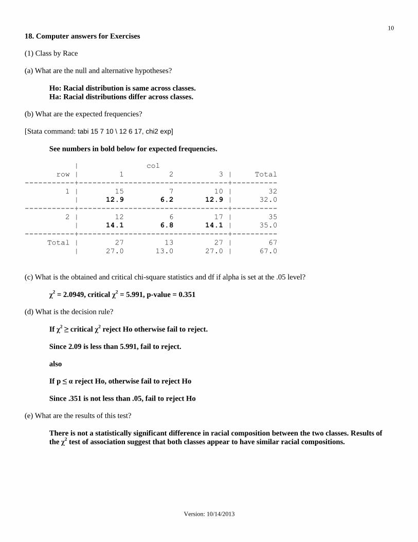
18. Computer answers for Exercises
(1) Class by Race
(a) What are the null and alternative hypotheses?
Ho: Racial distribution is same across classes.
Ha: Racial distributions differ across classes.
(b) What are the expected frequencies?
[Stata command: tabi 15 7 10 \ 12 6 17, chi2 exp]
See numbers in bold below for expected frequencies.
| col
row | 1 2 3 | Total
-----------+---------------------------------+----------
1 | 15 7 10 | 32
| 12.9 6.2 12.9 | 32.0
-----------+---------------------------------+----------
2 | 12 6 17 | 35
| 14.1 6.8 14.1 | 35.0
-----------+---------------------------------+----------
Total | 27 13 27 | 67
| 27.0 13.0 27.0 | 67.0
(c) What is the obtained and critical chi-square statistics and df if alpha is set at the .05 level?
χ2 = 2.0949, critical χ
2 = 5.991, p-value = 0.351
(d) What is the decision rule?
If χ2 ≥ critical χ
2 reject Ho otherwise fail to reject.
Since 2.09 is less than 5.991, fail to reject.
also
If p ≤ α reject Ho, otherwise fail to reject Ho
Since .351 is not less than .05, fail to reject Ho
(e) What are the results of this test?
There is not a statistically significant difference in racial composition between the two classes. Results of
the χ2 test of association suggest that both classes appear to have similar racial compositions.
11
Version: 10/14/2013
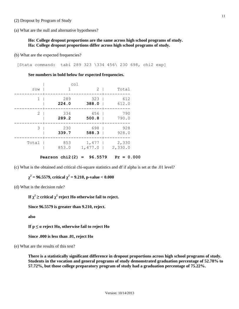
(2) Dropout by Program of Study
(a) What are the null and alternative hypotheses?
Ho: College dropout proportions are the same across high school programs of study.
Ha: College dropout proportions differ across high school programs of study.
(b) What are the expected frequencies?
[Stata command: tabi 289 323 \334 456\ 230 698, chi2 exp]
See numbers in bold below for expected frequencies.
| col
row | 1 2 | Total
-----------+----------------------+----------
1 | 289 323 | 612
| 224.0 388.0 | 612.0
-----------+----------------------+----------
2 | 334 456 | 790
| 289.2 500.8 | 790.0
-----------+----------------------+----------
3 | 230 698 | 928
| 339.7 588.3 | 928.0
-----------+----------------------+----------
Total | 853 1,477 | 2,330
| 853.0 1,477.0 | 2,330.0
Pearson chi2(2) = 96.5579 Pr = 0.000
(c) What is the obtained and critical chi-square statistics and df if alpha is set at the .01 level?
χ2 = 96.5579, critical χ
2 = 9.210, p-value < 0.000
(d) What is the decision rule?
If χ2 ≥ critical χ
2 reject Ho otherwise fail to reject.
Since 96.5579 is greater than 9.210, reject.
also
If p ≤ α reject Ho, otherwise fail to reject Ho
Since .000 is less than .01, reject Ho
(e) What are the results of this test?
There is a statistically significant difference in dropout proportions across high school programs of study.
Students in the vocation and general programs of study demonstrated graduation percentage of 52.78% to
57.72%, but those college preparatory program of study had a graduation percentage of 75.22%.

12
Version: 10/14/2013
(3) Success by Type of Feedback
(a) What are the null and alternative hypotheses?
Ho: Success of complex learning task is independent of feedback type.
Ha: Success of complex learning task differs across feedback type.
(b) What are the expected frequencies?
[Stata command: tabi 6 4 \4 6\ 8 2 \ 3 7, chi2 exp]
See numbers in bold below for expected frequencies.
| col
row | 1 2 | Total
-----------+----------------------+----------
1 | 6 4 | 10
| 5.3 4.8 | 10.0
-----------+----------------------+----------
2 | 4 6 | 10
| 5.3 4.8 | 10.0
-----------+----------------------+----------
3 | 8 2 | 10
| 5.3 4.8 | 10.0
-----------+----------------------+----------
4 | 3 7 | 10
| 5.3 4.8 | 10.0
-----------+----------------------+----------
Total | 21 19 | 40
| 21.0 19.0 | 40.0
Pearson chi2(3) = 5.9148 Pr = 0.116
(c) What is the obtained and critical chi-square statistics and df if alpha is set at the .01 level?
χ2 = 5.9148, critical χ
2 = 11.345, p-value = 0.116
(d) What is the decision rule?
If χ2 ≥ critical χ
2 reject Ho otherwise fail to reject.
Since 5.9148 is less than 11.345, fail to reject Ho.
also
If p ≤ α reject Ho, otherwise fail to reject Ho
Since .116 is greater than .01, fail to reject Ho
(e) What are the results of this test?
There is not a statistically significant difference in complex learning task success rates across feedback
conditions. Results suggest that student success at learning a complete learning task are similar no matter
which learning condition they experienced.