CHERN-WEIL THEORY

ADEL RAHMAN

Abstract. We give an introduction to the Chern-Weil construction of char-

acteristic classes of complex vector bundles. We then relate this to the more

classical notion of Chern classes as described in [2].

Contents

1. Introduction 11.1. Conventions 22. Chern-Weil Theory: Invariants from Curvature 32.1. Constructing Curvature Invariants 63. The Euler Class 74. The Chern Class 104.1. Constructing Chern Classes: Existence 104.2. Properties 114.3. Uniqueness of the Chern Classes 145. An Example: The Gauss-Bonnet Theorem 166. Describing the Curvature Invariants 17Appendix A. Sums and Products of Vector Bundles 18Appendix B. Connections and Curvatures of Complex Vector Bundles 19Appendix C. Complex Grassmann Manifolds 21Acknowledgments 22References 22

1. Introduction

One of the fundamental problems of topology is that of the classification of topo-logical spaces. Algebraic topology helps provide useful tools for this quest by meansof functors from topological spaces into algebraic spaces (e.g. groups, rings, andmodules). By ensuring that these functors are suitably invariant under topologi-cally irrelevant deformation (e.g homeomorphism, or often just the weaker notionof homotopy equivalence), these functors provide us with a means by which toclassify spaces—if the targets of two spaces don’t match, then they are surely nothomeomorphic (precisely due to this invariance property).

Characteristic classes provide us with a tool of the same nature, but for the morespecialized notion of fibre bundles. A characteristic class is a map c from a bundleξ = (E, π,B) into the cohomology of B, c : ξ → H∗(B) that satisfies a naturality

Date: September 26, 2017.

1

2 ADEL RAHMAN

condition, c(ξ) = f∗c(ξ′) for any bundle map f : ξ → ξ′. It is this naturality con-dition which ensures that characteristic classes are invariant under vector bundleisomorphism, and thus capture information about the isomorphism class of a vectorbundle. In this way they provide us with a new classification tool—if two bundlesdo not have the same sets of characteristic classes, they are surely not isomorphic.

It was shown by Chern and Weil in the late 1940’s that one can in fact constructsuch characteristic classes in the case of complex plane bundles using geometricaldata—in particular connections and their curvatures. This is of remarkable use inphysics, where complex vector bundles arise as the playground of quantum fields(operator valued sections of complex vector bundles). These bundles are often pre-scribed with a connection A, called the “gauge field”, which has a curvature Fcalled the “field strength”. The work of Chern and Weil tells us that we can useF alone to construct the characteristic classes of this bundle. Thus every quantumgauge theory comes prescribed with a way to understand its underlying topology.The properties of the characteristic classes of these bundles, in turn, constrain thephysical theory, giving rise to such phenomena as the Bohm-Aharonov effect. Con-versely, any gauge theory which does not depend on the metric of the underlyingspacetime manifold must have a Lagrangian which depends only on “topologicalterms”. These “topological terms” are precisely the characteristic classes of therelevant bundles.

In this paper we will review the construction of Chern and Weil, and then showthat we can in fact construct all characteristic classes of complex plane bundles(satisfying certain axioms) in this way. We begin in Section 2 by reviewing theconstruction of characteristic classes from curvatures. We then review the relevanttopological theory of characteristic classes to show that the previous constructiondoes indeed give us what we want. In Section 3 we consider the Euler class of anoriented real bundle and in Section 4 use this to construct the Chern classes of acomplex plane bundle. In this same section we show that any characteristic class ofa complex plane bundle satisfying a certain set of simple axioms must be a Chernclass. Armed with this uniqueness theorem, we proceed in Section 5 to relate ourinitial geometrically constructed invariants to the Chern classes.

Throughout this paper we will assume familiarity with the theory of smoothmanifolds and some elementary algebraic topology. In particular, we will assumefamiliarity with vector bundles and cohomology theory. Readers unfamiliar withthe notion of connections and their associated curvatures may refer to AppendixB. Appendix A reviews some basic vector bundle constructions, and Appendix Creviews the theory of complex Grassmann manifolds and their utility in providingclassifying spaces for complex plane bundles.

1.1. Conventions. All manifolds will be smooth, Hausdorff, and paracompact.

Bundles will be denoted by triples ζ = (E, π,M) or by the standard Eπ−→M . We

will use Γ(ζ) to denote the space of smooth sections of a bundle ζ. Unless otherwisespecified, all functions should be assumed smooth.

CHERN-WEIL THEORY 3

For any bundle ζ = (E, π,M), E0 will denote the space obtained by removingthe zero section from E.

We will use the sign convention of [2] (Milnor & Stasheff) for the definition ofthe coboundary δ, i.e.

〈δc, α〉 = (−1)n+1 〈c, ∂α〉for [c] ∈ Hn(X; Λ), [α] ∈ Hn+1(X; Λ) (X some space and Λ some ring).

With this convention, for example, Stokes’ theorem reads

〈dω, µ〉 = (−1)dim M 〈ω, ∂µ〉and thus our volume forms will differ from the standard volume forms by a sign

volour = (−1)dimMvolstd

To return to the standard conventions for coboundaries and volumes, send Ω→ −Ωin all characteristic class formulas involving the curvature that follow.

2. Chern-Weil Theory: Invariants from Curvature

Let ζ = (E, π,M) be a smooth, complex n-plane bundle. We denote the com-plexification of the cotangent bundle of M by (T ∗M)C as in Appendix B. We willhere use geometrical data (connections and curvatures) to construct useful topo-logical invariants of the bundle ζ.

Consider a connection ω on ζ with curvature Ω. Then Ω is a (gl(n,C)-valued)two-form on M . Our goal is to use the two-form character of Ω to obtain a mapfrom ζ into the de Rham cohomology of M . We want this construction to be in-dependent of the choice of connection (since the space of all connections on ζ iscontractible, and the de Rham cohmology functor is homotopy invariant), and thusproduce invariants of the bundle itself.

Our first task is to isolate the differential form character of Ω from its matrixcharacter.

Let M(n,C) denote the space of n× n complex matrices.

Definition 2.1. An invariant polynomial on M(n,C) is a function

P : M(n,C)→ Cwhich is basis invariant; i.e., which satisfies

P (TAT−1) = P (A)

for every nonsingular matrix T .

Proposition 2.2. The above property of basis independence is equivalent to cyclic-ity. In particular, for any invariant polynomial P , P (AB) = P (BA).

Proof. Let P be basis independent and letA, B be any matrices. IfB is nonsingular,then

P (AB) = P(B(AB)B−1

)= P (BA)

by basis independence. If B is singular, the result follows by the continuity of P ,since we may approximate B to arbitrary accuracy by nonsingular matrices. Thus

4 ADEL RAHMAN

P is cyclic.

Conversely, let P be cyclic and T be a nonsingular matrix. Then

P (A) = P (AI) = P (AT−1T ) = P (TAT−1)

and thus P is basis independent.

Thus any basis independent matrix is cyclic and vice-versa

Example 2.3. Both the determinant and the trace are invariant polynomials.

It is this machinery of invariant polynomials which precisely provides us with away to isolate the differential form character of Ω. This occurs as follows:

Given any curvature form Ω and any invariant polynomial P , we may define adifferential form P (Ω) in the following way. Consider an open cover of M , and ineach open set select a local basis of sections si. We may define the componentsΩij of our curvature form in this basis via

Ω(si) =∑j

Ωij ⊗ sj

where each Ωij is a 2-form. Regarding the curvature form as a matrix Ω = [Ωij ]whose entries lie in the commutative algebra of even-dimensional forms over C,we can evaluate P on Ω (precisely because of the commutativity of all elementsinvolved) to obtain a sum of forms of even degree. Since M is Hausdorff and para-compact, we may patch together the local representatives P (Ωij) into a global formusing a partition of unity. Since P is invariant, this form does not depend on ourchoices of local basis.

Note that we may just as easily replace our invariant polynomial P by a formalpower series

P = P0 + P1 + P2 + . . .

where each Pk is an invariant homogeneous polynomial of degree k.

The evaluation P (Ω) will always be well defined, since Pk(Ω) = 0 for 2k > dimM(since Pk(Ω) will be a differential form of degree 2k).

The following lemma shows that P (Ω) provides us with exactly what we sought—an element of the de Rham cohomology.

Lemma 2.4. For any invariant polynomial P , the form P (Ω) is closed.

Proof. Let P be an invariant polynomial and Ωij the components of Ω in some localbasis. We have that

dP (Ω) =∑ij

∂P

∂ΩijdΩij = tr (P ′(Ω) dΩ)

where we have introduced the matrix

[P ′(Ω)]ij =∂P

∂Ωji

CHERN-WEIL THEORY 5

Using thatΩ = dω − ω ∧ ω

we arrive at the Bianchi identity

dΩ = ω ∧ Ω− Ω ∧ ωwhich gives us the matrix of three-forms [dΩ].

We note that P ′(Ω) and Ω must commute, which may be seen by differentiatingboth sides of the following identity and evaluating at t = 0 (where [Eij ]kl = δikδjlis the matrix unit with (i, j)th component 1 and all other components zero)

P ((I + tEij)Ω) = P (Ω(I + tEij))

Taking the derivatives yields∑k

∂P

∂ΩikΩjk =

∑k

∂P

∂ΩkjΩki

Thus, in cohomology, we must have that

[P ′(Ω)] · [Ω] = [Ω] · [P ′(Ω)] =⇒ Ω ∧ P ′(Ω) = P ′(Ω) ∧ Ω

Substituting the Bianchi identity into our formula for dP (Ω) and using the gradedcyclicity of the trace (tr (α ∧ β) = (−1)|α||β|tr (β ∧ α)) gives us that

dP (Ω) = tr (P ′(Ω) ∧ ω ∧ Ω− P ′(Ω) ∧ Ω ∧ ω)

= tr (P ′(Ω) ∧ Ω ∧ ω − P ′(Ω) ∧ Ω ∧ ω) = 0

Thus P (Ω) is closed and is a (complex) de Rham cocycle, as we wished to show.

Thus every invariant polynomial P allows us to assign cohomology classes tocurvatures on ζ:

P : Ω 7→ [P (Ω)] ∈ H∗(M ;C)

We have the following lemma

Corollary 2.5. The cohomology class [P (Ω)] is independent of the connection ω.

Proof. Let ω0 and ω1 be two different connections on ζ. Considering the map

p1 : M × R→M (p, t) 7→ p

we may form the induced bundle ζ ′ := p∗1 ζ over M × R and induced connectionsω′i := p∗1 ωi on ζ ′. Note that the linear combination

ω := tω′1 + (1− t)ω′0is also a connection on ζ ′. Let Ω be the curvature of ω and Ωi the curvature ofeach ωi, and note that P (Ω) will be a de Rham cocycle on M × R.

We now consider the family of maps it : M → M × R defined by it : p 7→ (p, t),t ∈ [0, 1]. For t = 0, 1, we can identify the induced connections (it)

∗ω on (it)∗ζ ′

with the connections ωt on ζ. Thus

(it)∗[P (Ω)] = [P (Ωi)]

Since the mapping i0 is homotopic to i1, it follows that

[P (Ω1)] = [P (Ω2)]

6 ADEL RAHMAN

Thus we confirm what we initially suspected, that the mapping P : Ω 7→ [P (Ω)]determined a characteristic (cohomology) class of the bundle ζ in H∗(M ;C)(i.e. this class is characteristic of the bundle structure itself). Since any isomor-phism of bundles gives an isomorphism of base spaces (which in turn induces anisomorphism of cohomology), we see that this class can only depend on the isomor-phism class of ζ. Indeed, we have from the above that for any map g : M ′ → M ,we must have that

[P (Ω′)] = g∗[P (Ω)]

where Ω′ is the curvature of the induced connection on g∗ζ.

It is now natural to ask how this “newly discovered” invariant corresponds toother topological notions that have already been well studied (e.g. as the de Rhamcohomology of a manifold corresponds via de Rham’s theorem to its singular coho-mology and topological Betti numbers). We will see later that any such curvature“characteristic class” for a complex vector bundle can be expressed in terms of whatwill be called “Chern classes”.

We conclude this section by classifying these curvature invariants, later returningto the problem of expressing these invariants in terms the Chern classes.

2.1. Constructing Curvature Invariants. For any square (n × n) matrix A,define σk(A) to be the kth elementary symmetric function of the eigenvalues of A

σk(A) =∑

1≤i1<...in≤n

ai1 . . . aik

where the ai are the eigenvalues of A. We then have that

det(I + tA) =

∞∑k=0

tkσk(A)

Note that σk(A) = 0 for k > n so that the sum is finite.

Lemma 2.6. Any invariant polynomial on M(n,C) can be expressed as a polyno-mial function of σ1, . . . , σn.

Proof. Let A ∈ M(n,C) and B be the similarity transformation which takes A toits Jordan canonical form—i.e. BAB−1 is in Jordan canonical form and is thus, inparticular, upper triangular. Replace B with diag(ε, . . . , εn)·B for some ε arbitrarilyclose to 0 (so that the off diagonal terms of BAB−1 are correspondingly arbitrarilyclose to 0). By the continuity of P , it follows that P (A) = P (BAB−1) only dependson the diagonal entries of BAB−1, i.e. on the eigenvalues of A. Since P (A) must bysymmetric in these eigenvalues since if A = diag(a1, . . . , an) (as we may switch theordering of any two of the eigenvalues by a change of basis) it must be expressibleas a polynomial in the elementary symmetric functions (this is a classical resultfrom the theory of symmetric functions). Since σk(A) = 0 for k > n, the resultfollows.

We thus have found the building blocks, the elementary symmetric polynomialsσk, for any curvature invariant we can imagine (i.e. for any invariant polynomial

CHERN-WEIL THEORY 7

we can imagine). We will see that the “Chern classes” cr(ζ) will be related to ourcurvature invariants via

ck(ζ) =σk(Ω)

(2πi)k

We now take a detour into the classical theory of Chern classes before returningto the issue of understanding our curvature invariants fully.

3. The Euler Class

We now introduce the Euler class, both as a preliminary step towards the defi-nition of Chern classes, and as an independent demonstration of the constructionand utility of characteristic classes.

For any oriented manifold, there is a privileged element of the top cohomologygroup (with coefficients in Z): the fundamental cohomology class [u] (i.e. the dualto the fundamental homology class [µ] defined by 〈u, µ〉 = 1). In particular, this istrue for any oriented real vector space. Thus it is not unreasonable to believe that,if we can suitably extend the concept of orientation to real vector bundles, we maybe able to find cohomological invariants of these oriented bundles. This is preciselythe idea of the Euler class.

Definition 3.1. Let Eπ−→ B be a real n-plane bundle. An orientation on E is

a choice of orientation for each fiber such that each b ∈ B has a neighborhood Ubwith a local basis of sections si such that the orientation determined by si(b)agrees with that on Fb. Equivalently, we may require that b be contained in a localtrivialization (Ub, τ) such that the linear mapping v 7→ τ−1(b, v) from Rn to Fb isorientation preserving.

In terms of cohomology, this says that each fiber is assigned a preferred gener-ator uF ∈ Hn(F, F0;Z) and for each b ∈ B, there exists a neighborhood Ub and acohomology class ub ∈ Hn(π−1(Ub), π

−1(Ub)0;Z) such that for every fiber F overUb, the restriction ub|(F,F0) ∈ Hn(F, F0;Z) is equal to uF .

We have the following theorem:

Theorem 3.2 (Thom isomorphism). Let Eπ−→ B be a a real, oriented n-plane

bundle. The cohomology group Hi(E,E0;Z) is zero for i < n and Hn(E,E0;Z)contains a unique cohomology class u (the Thom class) such that the restrictions

u|(F,F0) ∈ Hn(F, F0;Z)

are equal to the fundamental classes uF for each fiber F . The correspondencey 7→ y∪u provides an isomorphism between Hk(E;Z) and Hk+n(E,E0;Z) for eachinteger k—i.e. H∗(E,E0;Z) is a free H∗(E;Z)-module on one degree-n generatoru.

For a proof, refer to chapter 10 of [2].

Since E deformation retracts onto its zero section (which is homeomorphic toB) via (t, v) 7→ tv, we have that Hk(B;Z) ' Hk(E;Z) (via π∗), and so the abovegives us further that

Hk(B;Z) ' Hn+k(E,E0;Z) x 7→ (π∗x) ∪ u

8 ADEL RAHMAN

We can now go forward with the definition of the Euler class.

Given an oriented n-plane bundle Eπ−→ B, the inclusion (E,Ø) ⊆ (E,E0) gives

rise to the restriction homomorphism

H∗(E,E0;Z)→ H∗(E;Z) y 7→ y|EApplying this homomorphism to the Thom class u ∈ Hn(E,E0;Z) gives an elementu|E of Hn(E;Z).

Definition 3.3. The Euler class of an oriented (real) n-plane bundle ξ = Eπ−→ B

is the cohomology class

e(ξ) ∈ Hn(B;Z)

given by

π∗e(ξ) = u|E

The name “Euler characteristic” comes from the fact that for any smooth, com-pact, oriented manifold M , the “Kronecker index” 〈e (TM) , µ〉 recovers the Eulercharacteristic, χ(M) of M .

The Euler class has the following properties:

Proposition 3.4 (Naturality).For all f : B → B′ covered by an orientation preserving bundle map ξ → ξ′,

e(ξ) = f∗e(ξ′)

Proposition 3.5 (Parity).If the orientation of ξ is reversed, the Euler class changes sign.

These results follow from the uniqueness of the Thom class and the parity prop-erty of the fundamental class (and hence the Thom class) respectively.

Example 3.6. Let ξ be a trival n-plane bundle M × Rn π−→ M . Consider thebundle map taking ξ to ξ′, the trivial n-plane bundle over a point

f : M × Rn → 0 × Rn

giving by mapping M to 0. This is clearly orientation preserving (it does not affectthe fibers). This covers π f , and so we must have that

e(ξ) = (π f)∗e(ξ′) = (π f)∗0 = 0

We also have the following proposition

Proposition 3.7.The Euler class of a Whitney sum or Cartesian product of bundles is given by

e(ξ ⊕ ξ′) = e(ξ) ∪ e(ξ′) e(ξ × ξ′) = e(ξ)× e(ξ′)

Remark 3.8. Note that the orientation of F ⊕ F ′ for two oriented vector spaces F ,F ′, is given by taking an oriented basis for F followed by an oriented basis for F ′.

Proof. Let ξ have fibers of dimension m and ξ′ have fibers of dimension n. Withour sign conventions, the fundamental class (and thus the Thom class) obeys

µ(ξ × ξ′) = (−1)mnµ(ξ)× µ(ξ′)

CHERN-WEIL THEORY 9

(under the isomorphism Hm+n(B × B′) ' Hm(B) × Hn(B′)). Applying the re-striction homomorphism

Hm+n(E × E′, (E × E′)0)→ Hm+n(E × E′) ' Hm+n(B ×B′)we get

e(ξ × ξ′) = e(ξ)× e(ξ′)Now suppose that B = B′. Pulling back both sides of the above equation via

the diagonal map B → B ×B to Hm+n(B;Z) gives us that

e(ξ ⊕ ξ′) = e(ξ) ∪ e(ξ′)

We now give two examples of properties of the Euler class which can extractuseful information about our bundles.

Lemma 3.9. If the fiber dimension n of ξ is odd, 2e(ξ) = 0

Proof. The Thom isomorphism maps e(ξ) to

π∗e(ξ) ∪ u = (u|E) ∪ u = u ∪ ui.e.

e(ξ) = φ−1(u ∪ u)

where φ is the Thom isomorphism. But

u ∪ u = (−1)(dimu)2u ∪ uso that u ∪ u, and hence e(ξ), is its own additive inverse whenever the dimensionof our space is odd.

Using this and the Whitney sum property, we can, for example, see that anybundle for which 2e(ξ) 6= 0 cannot be split as the Whitney sum of two oriented odddimensional vector bundles.

The following lemma encapsulates one of the most important properties of theEuler class

Lemma 3.10. Let ξ = (E, π,B) be real oriented vector bundle which possesses anowhere zero section. Then e(ξ) = 0.

Proof. Let s ∈ Γ(ξ) be a nonzero cross section. Since π s = id, the composition

Hn(B)π∗−→ Hn(E) −→ Hn(E0)

s∗−→ Hn(B)

must be the identity map of Hn(B). We note that under the first two maps, wemust have that

e(ξ) 7→ u|E 7→ (u|E)|E0

which must be zero since the composition

Hn(E,E0)→ Hn(E)→ Hn(E0)

is zero. Thus e(ξ) = s∗ [(u|E) |E0 ] = s∗(0) = 0.

Thus the existence of a nonzero Euler class provides an “obstruction” to theexistence of a nonzero section for an oriented real vector bundle ξ. This can beseen as the starting point for what is known as “obstruction theory”, which seeks tounderstand characteristic classes as obstructions to the existence of certain sectionsor structures on our bundles.

10 ADEL RAHMAN

4. The Chern Class

Armed with the notion of the Euler class, we now proceed to define the Chernclasses that we will use to classify our curvature invariants.

We will begin with a proof of a simple statement

Lemma 4.1. If ζ is a complex vector bundle, then the underlying real bundle ζRhas a canonical orientation.

Proof. Let V be a finite dimensional complex vector space with basis ej over C.Then the set e1, ie1, e2, ie2, . . . gives a real basis for the underlying real vectorspace VR. We note that this ordering (which determines the required orientation forVR) cannot depend on the initial choice of basis ei since GL(n,C) is connectedand thus all changes of basis continuous. We may apply this construction to eachfiber of ζ to obtain the required orientation of ζR.

Example 4.2. Let M be a complex manifold. Then, by the above, (TM)R iscanonically oriented. Since every orientation of the tangent bundle gives rise to aunique orientation of its base space, it follows that MR is canonically oriented aswell. But MR is topologically identical to M , and so M is canonically oriented aswell. Thus every complex manifold come equipped with a preferred orientation.

We note that the above implies that for any complex n-plane bundle ζ = (E, π,B),the Euler class

e(ζR) ∈ H2n(B;Z)

is automatically well defined. If ζ ′ is a complex m-plane bundle over the same basespace B, the Whitney sum property tells us that

e (ζ ⊕ ζ ′)R = e(ζR) ∪ e(ζ ′R)

since ζR⊕ ζ ′R is isomorphic to (ζ ⊕ ζ ′)R as oriented bundles (a preferred orientation

a1, ia1, . . . for π−1R (b) followed by a preferred orientation b1, ib1, . . . for π′−1R (b)

gives a preferred orientation a1, . . . , ian, b1, . . . for (π ⊕ π′)−1R (b)).

Recall that Hermitian metric on a complex vector space is a positive definitesesquilinear form. It may be defined as the unique inner product on the underlyingreal vector space which satisfies |iv| = |v| and is linear in the “first slot” (i.e. 〈w, · 〉is linear). As our base manifold B is paracompact, every complex vector bundleover B will admit a Hermitian metric (we may cover ζ with a local trivialization,define a metric on each element of the cover, and patch these together with a par-tition of unity).

4.1. Constructing Chern Classes: Existence. Let ζ = (E, π,M) be a com-plex n-plane bundle equipped with a Hermitian metric h. We will preliminarilyconstruct a canonical (n − 1)-plane bundle, ζ0, over the “deleted total space” E0

of all nonzero vectors in E, whose fiber over a point (p, v) in E0 is given by theorthogonal complement of v in π−1(p) under h.

CHERN-WEIL THEORY 11

We note that for any n-plane bundle Eπ−→ M there is associated a long exact

sequence in cohomology with integer coefficients (denoting π0 := π|E0):

· · · → Hi(B)∪e−→ Hi+n(B)

π∗0−→ Hi+n(E0)→ Hi+1(B)∪e−→ . . .

the Gysin sequence. A proof of the existence of this sequence can be found inchapter 8 of [2].

For i < 2n−1, both the groups Hi−2n(B) and Hi−2n+1(B) zero, and so we musthave that π∗0 : H(B)→ Hi(E0) is an isomorphism.

We may now use the above isomorphism to recursively define the Chern classes.

Definition 4.3. We define the Chern classes ci(ζ) ∈ H2i(B;Z) recursively asfollows, inducting on the complex dimension n of ζ.

For i > n, we set ci(ζ) = 0. The top Chern class cn(ζ) is equal to the Eulerclass of the underlying real bundle, i.e.

cn(ζ) = e(ζR) ∈ H2n(B;Z)

For i < n, recalling the map (π∗0)−1 : H2i(E0)→ H2i(B), we set

ci(ζ) = (π∗0)−1ci(ζ0)

For example, this setscn−1(ζ) = (π∗0)

−1e(ζ0,R)

and so on. Note that in particular this gives c0(ζ) = 1.

Definition 4.4. The formal sum

c(ζ) =

n∑i=1

ci(ζ) ∈⊕i

Hi(B;Z)

is called the total Chern class of ζ. This is a unit with well defined inverse.

4.2. Properties. The Chern classes have the following properties:

Proposition 4.5 (Naturality). If f : B → B′ is covered by a bundle map from acomplex n-plane bundle ζ to another complex n-plane bundle ζ ′, then

c(ζ) = f∗c(ζ ′)

Proof. We know that this holds for the top Chern class, since this is just the Eulerclass. To prove naturality for the lower classes, we note that the bundle map ζ → ζ ′

gives rise to a unique map f0 : E0(ζ)→ E0(ζ ′), which is in turn covered by a bundlemap ζ0 → ζ ′0. Thus we must have that ci(ζ0) = f∗0 ci(ζ

′0), again by the naturality

of the Euler class. We now appeal to the following commutative diagram

E0(ζ)f0 //

π0

E0(ζ ′)

π′0

Bf

// B′

as well as the identities ci(ζ0) = π∗0ci(ζ) and ci(ζ′0) = π′∗0 ci(ζ

′) where π∗0 is anisomorphism for i < n. Thus we must have that ci(ζ) = f∗ci(ζ

′) as required.

12 ADEL RAHMAN

Proposition 4.6 (Sum Formula). Let ζ and ξ be two complex vector bundles overa common paracompact base space B. Then

c(ζ ⊕ ξ) = c(ζ) ∪ c(ξ)

As a first step towards proving this, we prove the following lemma

Lemma 4.7. There exists one and only one polynomial

pm,n(c1, . . . , cm; c′1, . . . , c′n)

with integer coefficients in m+ n indeterminates such that

c(ζ ⊕ ξ) = pm,n(c1(ζ), . . . , cm(ζ); c1(ξ), . . . , cn(ξ)

holds for every complex m-plane bundle ζ and n-plane bundle ξ over a commonparacompact base space.

Proof. This proof is important since it gives an example of the utility of the Grass-mann manifolds and canonical bundles discussed in Appendix C The reader unfa-miliar with the use of the canonical bundles over the complex Grassmann manifoldsas classifying spaces is encouraged to reference that appendix before continuing onwith this proof.

We will construct the following two bundles, γm1 and γn2 over Gm × Gn as uni-versal models for pairs of complex vector bundles. We define γm1 := π∗1γ

m andγn2 := π∗2γ

n where π1 : Gm ×Gn → Gm is projection onto the first factor and simi-larly for π2. Thus the Whitney sum γm1 ⊕ γn2 can be identified with the Cartesianproduct.

Noting that the external cohomology cross-product operation

a, b 7→ a× b = π∗1a ∪ π∗2binduces an isomorphism between H∗(Gm;Z) ⊗ H∗(Gn;Z) and H∗(Gm × Gn;Z)(which follows from the Kunneth isomorphism).

Using (C.5), we see that H∗(Gm×Gn) is a polynomial ring over Z on generatorsπ∗1ci(γ

m) = ci(γm1 ) and π∗2cj(γ

n) = cj(γn2 ). Thus the total Chern class of γm1 ⊕ γn2

can be expressed uniquely as a polynomial

c(γm1 ⊕ γn2 ) = pm,n (c1(γm1 ), . . . , cm(γm1 ); c1(γn2 ), . . . , cn(γn2 ))

Now as ζ is a complex m-plane bundle and ξ a complex n-plane bundle,both overB, we can choose maps f : B → Gm and g : B → Gn (recall (C.3)) so that

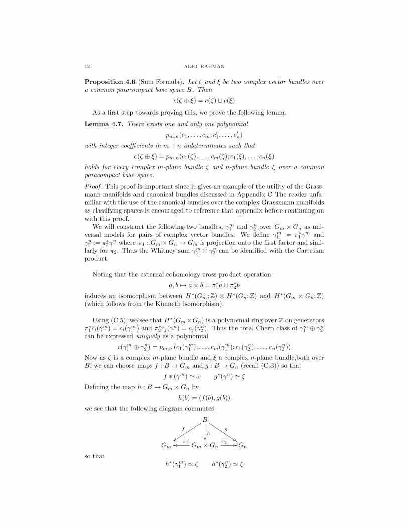
f ∗ (γm) ' ω g∗(γn) ' ξDefining the map h : B → Gm ×Gn by

h(b) = (f(b), g(b))

we see that the following diagram commutes

Bf

yyh

g

$$Gm Gm ×Gn

π1oo π2 // Gn

so thath∗(γm1 ) ' ζ h∗(γn2 ) ' ξ

CHERN-WEIL THEORY 13

and thus

c(ζ ⊕ ξ) = h∗c(γm1 ⊕ γn2 )

= pm,n(c1(ζ), . . . , cm(ζ); c1(ξ), . . . , cn(ξ)

We now compute these polynomials, proceeding by induction of m+n. We makeuse of the following lemma

Lemma 4.8. If εk is the trivial complex k-plane bundle over B, then c(ζ⊕εk) = c(ζ)for all complex vector bundles ζ over B.

Proof. It suffices to prove the lemma for the case k = 1 since the rest will follow byinduction. Letting ξ = ζ ⊕ ε1, we note that ξ has a nonzero section s : p 7→ (0, α)where α is some fixed complex number. Thus we must have that (letting ζ havefiber dimension n)

cn+1(ξ) = e(ξR) = 0 = cn+1(ξ)

We note that s : B → E0(ξ) is covered by a bundle map ζ → ξ0 so that

s∗ci(ξ0) = ci(ζ)

by naturality. Substituting π∗0ci(ξ) for ci(ξ0) and using that s∗ π∗0 = id gives usthat ci(ξ) = ci(ζ) as required.

We now complete our computation, which will in turn prove the initial proposi-tion.

Proof of Proposition 5.6. Suppose inductively that c(γm−11 ⊕γn2 ) = c(γm−11 )∪c(γn2 )(the base case m,n = 1 is clear). We then consider the bundles γm−11 ⊕ ε1 and γn2over Gm−1 ×Gn. On one hand we have that

c(γm−11 ⊕ ε1 ⊕ γn2 ) = pm,n(c1(γm−11 ⊕ ε1), . . . , cm(γm−11 ⊕ ε1); c1(γn2 ), . . . , cn(γn2 )

)whereas on the other, in light of the above lemma, we have that

c(γm−11 ⊕ ε1 ⊕ γn2 ) = pm,n(c1(γm−11 ), . . . , 0; c1(γn2 ), . . . , cn(γn2 )

)= c(γm−11 ⊕ γn2 )

Letting ci := ci(γm−11 ) and c′j := cj(γ

n2 ) and comparing with the induction hypoth-

esis, we find that

pm,n(c1, . . . , cm−1, 0; c′1, . . . , c′n) = c(γm−11 )c(γn2 ) = (1+c1+· · ·+cm−1)(1+c′1+· · ·+c′n)

(cup products understood). Introducing an indeterminate cm we have that

pm,n(c1, . . . , cm; c′1, . . . , c′n) = (1 + c1 + · · ·+ cm)(1 + c′1 + · · ·+ c′n) mod cm

A similar inductive argument shows that the two polynomials are also congruentmod c′n, i.e.

pm,n(c1, . . . , cm; c′1, . . . , c′n) = (1 + c1 + · · ·+ cm)(1 + c′1 + · · ·+ c′n) + fcmc

′n

for some polynomial z. We note that f must be zero degree (i.e. an integer) sinceotherwise γma ⊕ γn2 would have a nonzero Chern class in dimensions greater than2(m+ n).

14 ADEL RAHMAN

The above formula implies that

cm+n(ζ ⊕ ξ) = (1 + z)cm(ζ) ∪ cn(ξ)

but the top Chern class is just the Euler class of the underlying real bundle, whichalready has the sum property

cm+n(ζ ⊕ ξ) = e((ζ ⊕ ξ)R)

= e(ζR ⊕ ξR)

= e(ζR) ∪ e(ξR)

= cm(ζ) ∪ cn(ξ)

Hence z = 0 and we have proved the sum formula.

Corollary 4.9. Let ζ and ξ be two complex vector bundles over a common para-compact base space B. Then

ci(ζ ⊕ ξ) =∑j+k=i

cj(ζ) ∪ ck(ξ)

Proof. On one hand we have that

c(ζ ⊕ ξ) =

n+m∑i=1

ci(ζ ⊕ ξ)

whereas on the other we have that

c(ζ ⊕ ξ) = c(ζ) ∪ c(ξ) = [1 + c1(ζ) + · · ·+ cn(ζ)] ∪ [1 + c1(ξ) + · · ·+ cm(ξ)]

Equating orders of elements in cohomology gives

ci(ζ ⊕ ξ) =∑j+k=i

cj(ζ) ∪ ck(ξ)

as desired.

4.3. Uniqueness of the Chern Classes. We now turn to the question of theuniqueness of the Chern classes. We begin by noting that the Chern classes can becharacterized by the following axioms:

Let ζ = (E, π,B) a complex n-plane bundle.

(1) For each natural number i, there is a Chern class ci ∈ H2i(B;Z) withc0(ζ) = 1 and ci(ζ) = 0 for i > n.

(2) Naturality(3) Sum Formula(4) For the universal line bundle γ1 over G1 = CP∞, we have that

c1(γ1) = e((γ1)R)

)We now wish to show that it can uniquely be characterized by these four axioms,

i.e. that the Chern classes are uniquely characterized by the above axioms.

We must introduce a bit of machinery to do this.

Definition 4.10. Let ζ be a vector bundle over B. A splitting map for ζ is amap f : B′ → B such that f∗ζ is a Whitney sum of line bundles and f∗ : H∗(B)→H∗(B′) is injective.

CHERN-WEIL THEORY 15

We note that such maps actually do exist.

Proposition 4.11. Any n-plane bundle ζ over B has a splitting map.

A proof may be found in [1].

We have the following corollary

Corollary 4.12. If ζiki=1 are vector bundles over B, then there exists a mapf : B′ → B which is a splitting map for all the vector bundles ζi

Proof. We prove the above by induction on k. Clearly the above holds for thecase of one bundle. We assume that it holds for the case of k − 1 bundles andconsider the case of k bundles. Let each bundle ζi have fiber dimension n(i). Thereexists a map g : B′ → B such that g∗ : H∗(B) → H∗(B′) injective and withg∗ζi ' λi,1⊕ · · · ⊕ λi,n(i) for i < k where the λ’s are line bundles. There also existsa splitting map f : B′′ → B′ for the bundle g∗ζk. But then g f : B′′ → B is asplitting map for all the ζiki=1.

We now prove that the above axioms completely characterize the Chern classes.

Theorem 4.13 (Uniqueness). Let c′i be another sequence of characteristic classeswhich satisfies the above axioms 1)− 4). Then

c′i(ζ) = ci(ζ)

for any complex vector bundle ζ.

Proof. By axiom 4), we must have that c1(γ1) = c′1(γ1). Thus by naturality, wemust have that c1(λ) = c′(λ) for any line bundle λ. Now if ζ is a complex n-bundleover a paracompact base space B, we can find a splitting map f : B′ → B so thatf∗ is injective on cohomology and

f∗ζ ' λ1 ⊕ · · · ⊕ λn

for some line bundles λi. Applying the Whitney sum formula and the fact that cand c′ coincide on line bundles gives that

ci(f∗ζ) = c′i(f

∗ζ)

for all i and hence

f∗ci(ζ) = f∗c′i(ζ)

for all i. Since f∗ is injective, we must have that

ci(ζ) = c′i(ζ)

for all i. Hence the Chern class is unique.

Corollary 4.14. The first Chern class is the unique (modulo scalar multiplication)nontrivial characteristic class of a complex line bundle.

We now return to the issue of understanding our curvature invariants.

16 ADEL RAHMAN

5. An Example: The Gauss-Bonnet Theorem

With the Chern class now in hand, we return to the Chern-Weil theory to ex-plicitly construct a curvature invariant. Along the way, we will give a new prooffor a familiar theorem from the classical differential geometry of surfaces.

Consider a closed, oriented Riemannian two-manifold S. In two dimensions, theLevi-Civita curvature of M is given by

Ωij = K dA

where K is the Gaussian curvature of M .

In any neighborhood U of S we may introduce geodesic coordinates (x, y) inwhich the metric takes the form

g = dx⊗ dx+ g(x, y)2 dy ⊗ dySetting

θ1 = dx θ2 = g(x, y)dy

gives us a local orthonormal basis of forms over U , for which we can consider theequations of structure

0 = dθ1 = ω12 ∧ θ2 = g(x, y)ω12 ∧ dy∂g(x, y)

∂xdx ∧ dy = dθ2 = ω21 ∧ θ1 = −ω12 ∧ θ1 = −ω12 ∧ dx

Thus the connection form is given by

ω12 =∂g

∂xdy

so that

Ω12 =∂2g

∂x2dx ∧ dy =

1

g

∂2g

∂x2dθ1 ∧ dθ2 = −1

g

∂2g

∂x2dA

(recall our conventions for volume forms as given in section 1.1). Thus we havethat

K = −1

g

∂2g

∂x2

We may now use our thus developed machinery to prove the celebrated Gauss-Bonnet theorem.

Theorem 5.1 (Gauss-Bonnet). Let M be a closed, oriented Riemannian 2-manifold.Then ∫

M

Ω12 =

∫M

K dA = 2π〈e(TM), µ〉 = 2πχ(M)

Proof. The orientation on M gives rise to an orientation of each of the fibers of TM ,which we may view as an oriented 2-plane bundle with a Euclidean metric. Beforespecializing to TM , let’s first consider an arbitrary oriented, real 2-plane bundle ξ.ξ has a canonical complex structure J which rotates a vector “counterclockwise”through an angle of π/2—i.e. in terms of any oriented local orthonormal basis si,Js1 = s2. We may thus canonically identify ξ with a complex line bundle ζ whichinherits a connection obeying

∇s1 = ω12 ⊗ s2 = ω12 ⊗ (is1) = i ω12 ⊗ s1

CHERN-WEIL THEORY 17

so that∇(is1) = −ω12 ⊗ s1

so that the connection one form on ζ is given by

ωζ = i ω12

and thus the curvature matrix on ζ by

Ωζ = iΩ12

Using the invariant polynomial σ1 = tr , we obtain a cohomology class

[tr (iΩ12)] = [iΩ12] ∈ H2(M ;C)

This represents a characteristic class for ζ, but we know that there only exists one:the Chern class. Thus

iΩ12 = α c1(ζ) = α e(ξ)

for some α ∈ C. To evaluate α, it suffices to check a single case.

We thus return to the case of TM . Since iΩ12 = α e(TM), we must have that

i

∫M

K dA =

∫M

iΩ12 = α〈 e(TM), µ 〉 = αχ(M)

We now evaluate both sides for a sphere, for which K = 1, to get

4πi = 2α

hence α = 2πi. Hence ∫M

K dA = 2πξ(M)

and the theorem is proved.

6. Describing the Curvature Invariants

We would finally like to show how to express our curvature invariants in termsof the Chern classes. This is done by the following theorem

Theorem 6.1. Let ζ be a complex vector bundle with connection ω (and corre-sponding curvature Ω). Then the cohomology class σk(Ω) is equal to (2πi)kck(ζ).

Proof. Our proof of the Gauss-Bonnet theorem from the last section shows us thatthe theorem holds for all line bundles. To show the general case, we define theinvariant polynomial P by

P (A) = det (I +A/2πi) =∑k

σk(A)

(2πi)k

For a complex line bundle λ, we must have that

[P (Ωλ)] = [1 + σ1/2πi] = c(λ) = 1 + c1(λ)

Now consider any bundle which ζ which splits as a Whitney sum of line bundles

ζ = λ1 ⊕ · · · ⊕ λnChoosing connections ωi on λi, we get a unique sum connection ω on ζ. Choosinglocal sections si on each λi, the collection si gives a local basis of sections of ζ.The corresponding curvature matrix is diagonal

Ω = diag (Ω1, . . . ,Ωn)

18 ADEL RAHMAN

and hence

P (Ω) = P (Ω1) ∧ · · · ∧ P (Ωn)

by the multiplicative property of the determinant. But we have that

[P (Ω1) ∧ · · · ∧ P (Ωn)] = c(λ1) ∪ · · · ∪ c(λn) = c(ζ)

by the Whitney sum formula. Hence the result holds for any sum of line bundles.

However, we know that for any ζ, there exists a splitting map f that takes ζ toa sum of line bundles, and hence the result holds for f∗ζ, but since f∗ is injective,it must hold for any ζ.

Thus we see that, given any complex vector bundle and any connection on it, wecan construct its Chern classes using the invariant polynomials det(I + Ω/2πi).

We have finally shown that given just the geometrical data of a connection on acomplex n-plane bundle ζ, we may find all its characteristic classes. This gives usa bridge from the rigid geometry of a bundle back to its underlying topology.

Appendix A. Sums and Products of Vector Bundles

All proofs for the material of the appendices may be found in [2]. In this appen-dix, we recall the definitions of the Cartesian product and Whitney sum (i.e. directsum) of vector bundles.

Definition A.1. Let ξi = (Ei, πi, Bi)ni=1 be a finite collection of vector bundles.The Cartesian product of the bundles ξi defined as the bundle

ξ1 × · · · × ξn = (E1 × · · · × En, π1 × · · · × πn, B1 × · · · ×Bn)

with fibers

(π1 × · · · × πn)−1

(b1, . . . , bn) = π−11 (b1)× · · · × π−1n (bn)

given the structure of a Cartesian product of vector spaces.

Example A.2. T (M1×M2) ' TM1×TM2 where the isomorphism is taken as anisomorphism of bundles.

Definition A.3. Let ξ1 and ξ2 be two bundles over the same base space B. Denoteby d : B → B ×B the diagonal embedding. The bundle

ξ1 ⊕ ξ2 := d∗(ξ1 × ξ2)

is called the Whitney sum of ξ1 and ξ2 with each fiber π−1⊕ (b) canonically iso-

morphic to the direct sum π−11 (b)⊕ π−12 (b).

Example A.4. The exterior algebra of differential forms over a manifold M livesin the bundle

Λ (T ∗M) = ⊕nk=0

Λk (T ∗M)

CHERN-WEIL THEORY 19

Appendix B. Connections and Curvatures of Complex VectorBundles

Consider a vector bundle Eπ−→M . One of the shortcomings of the vector bun-

dle structure is that we are a priori provided with no way to compare the valuesof a section s ∈ Γ(E) at two different points (say p and q). The reason for this issimple: π−1(p) and π−1(q) are two different vector spaces, and there is no canonicalisomorphism between them.

It is clear that, were we given some way to unambiguously lift a curve γ on M(connecting p = π(v) and q) to a curve on E starting at v (connecting v ∈ π−1(p)to C(v, γ) ∈ π−1(q)), we could obtain a (curve-dependent) identification of thefibers π−1(p) and π−1(q) (in particular, we would want this implicit map C( · , · )to be linear and injective in the first “slot” and smooth in the second). Such aprescription for a curve-dependent identification of fibers is called a connection.

It is also clear that being provided with a connection should give us an unam-biguous was to take directional derivatives of sections along tangent vectors in M :we simply lift the curve along which we wish to take this derivative (i.e. whosetangent at parameter t = 0 is the tangent vector γ in question), and consider thelimit

∇γs = limt→0

s(γ(t))− C(s(γ(t)), γ−1(t)

)t

Similarly, any prescription for “covariantly” (i.e. independent of choice of co-ordinates or trivialization) taking derivatives defines a connection, since we mayidentify a vector s(p) with its “parallel transports” along γ, s(q) defined by

∇γs = 0

Thus we will sometimes abuse terminology and call a covariant derivative operatora connection and vice-versa.

Any connection on a principal fiber bundle can be described by a lie algebravalued one form ω, which descends to a one form on each of its associated bundles.Thus all connections on our vector bundles can be specified by an End(E) valuedone form ω, where E is the total space.

For our purposes, let ζ = Eπ−→ M be a smooth, complex n-plane bundle with

smooth (m dimensional) base space M . We denote by (T ∗M)C = HomR(TM,C)the complexification of the cotangent bundle (i.e. each fiber of (T ∗M)C is the com-plexification T ∗pM ⊗R C of the corresponding cotangent space). It is clear that(T ∗M)C ⊗C ζ will be a smooth, complex m+ n plane bundle over M .

Definition B.1. A connection ∇ on ζ is a C-linear mapping

∇ : Γ(ζ)→ Γ((T ∗M)C ⊗ ζ)

which satisfies the Leibniz rule:

∇(fs) = df ⊗ s+ f∇s

20 ADEL RAHMAN

for all s ∈ Γ(ζ), f ∈ C∞(M,C). The image∇s of a section s is called the covariantderivative of s.

Proposition B.2. The mapping s 7→ ∇s decreases supports (that is ∇s vanisheson any open region in which s vanishes).

Any local mapping L : Γ(ζ) → Γ(η) which decreases supports is called a localoperator since the value of L(s) at a point p only depends on the values of s inan arbitrarily small neighborhood of p. A theorem of Peetre assert that every localoperator is a differential operator, i.e. that it can be expressed locally as a finitelinear combination of partial derivatives with coefficients in Γ(η). This is where theone form ω comes in.

In any local trivialization, we may find a basis of sections si. We may alwayswrite

∇(si) =∑

ωij ⊗ sjfor some unique matrix of one forms ωij . This matrix ωij is just the representativeof the one form ω in this basis.

We have the following results about sections on ζ.

Proposition B.3. Let ∇1 and ∇2 be two connections on ζ and g any smoothcomplex valued function on M . Then g∇1 + (1− g)∇2 is another connection on ζ.In particular, the space of all connections on ζ is contractible.

Proposition B.4. Any smooth complex vector bundle with paracompact base spaceposesses a connection.

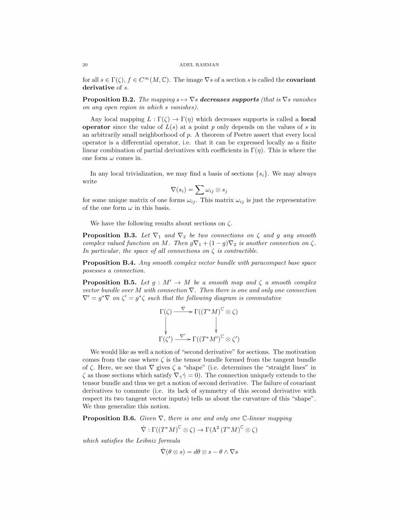
Proposition B.5. Let g : M ′ → M be a smooth map and ζ a smooth complexvector bundle over M with connection ∇. Then there is one and only one connection∇′ = g∗∇ on ζ ′ = g∗ζ such that the following diagram is commutative

Γ(ζ)∇ //

Γ((T ∗M)C ⊗ ζ)

Γ(ζ ′)

∇′ // Γ((T ∗M ′)C ⊗ ζ ′)

We would like as well a notion of “second derivative” for sections. The motivationcomes from the case where ζ is the tensor bundle formed from the tangent bundleof ζ. Here, we see that ∇ gives ζ a “shape” (i.e. determines the “straight lines” inζ as those sections which satisfy ∇γ γ = 0). The connection uniquely extends to thetensor bundle and thus we get a notion of second derivative. The failure of covariantderivatives to commute (i.e. its lack of symmetry of this second derivative withrespect its two tangent vector inputs) tells us about the curvature of this “shape”.We thus generalize this notion.

Proposition B.6. Given ∇, there is one and only one C-linear mapping

∇ : Γ((T ∗M)C ⊗ ζ)→ Γ(Λ2 (T ∗M)

C ⊗ ζ)

which satisfies the Leibniz formula

∇(θ ⊗ s) = dθ ⊗ s− θ ∧∇s

CHERN-WEIL THEORY 21

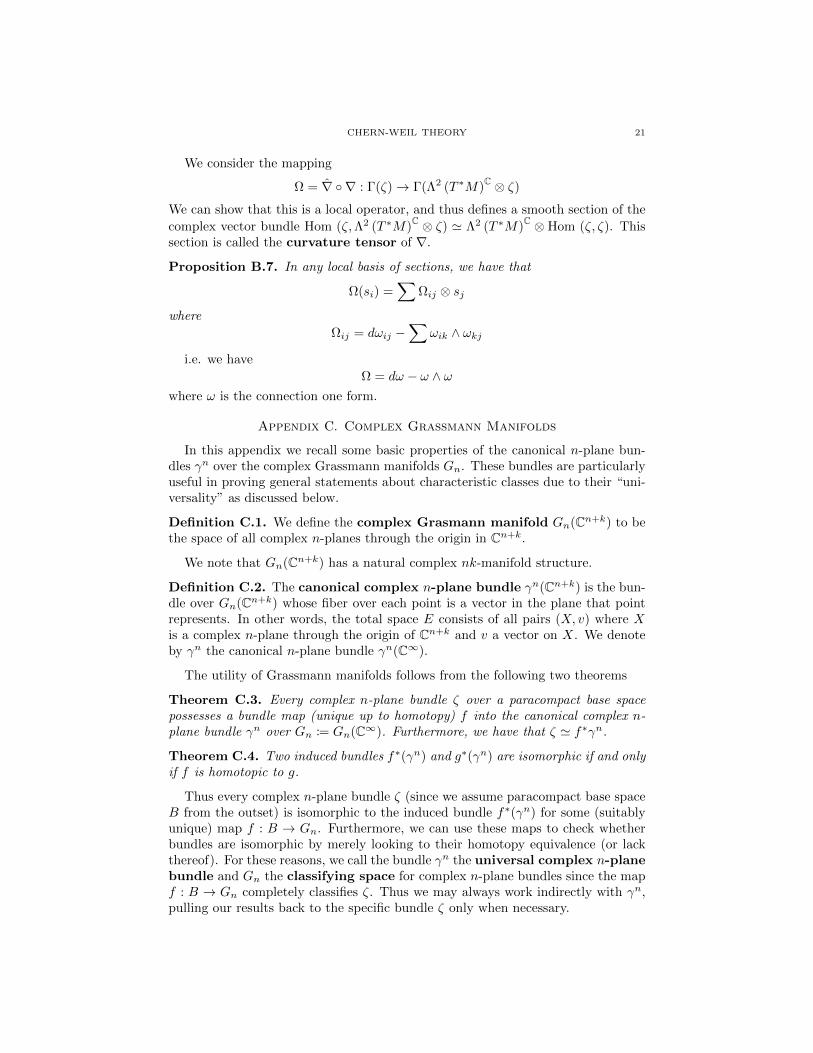
We consider the mapping

Ω = ∇ ∇ : Γ(ζ)→ Γ(Λ2 (T ∗M)C ⊗ ζ)

We can show that this is a local operator, and thus defines a smooth section of the

complex vector bundle Hom (ζ,Λ2 (T ∗M)C ⊗ ζ) ' Λ2 (T ∗M)

C ⊗ Hom (ζ, ζ). Thissection is called the curvature tensor of ∇.

Proposition B.7. In any local basis of sections, we have that

Ω(si) =∑

Ωij ⊗ sjwhere

Ωij = dωij −∑

ωik ∧ ωkj

i.e. we have

Ω = dω − ω ∧ ωwhere ω is the connection one form.

Appendix C. Complex Grassmann Manifolds

In this appendix we recall some basic properties of the canonical n-plane bun-dles γn over the complex Grassmann manifolds Gn. These bundles are particularlyuseful in proving general statements about characteristic classes due to their “uni-versality” as discussed below.

Definition C.1. We define the complex Grasmann manifold Gn(Cn+k) to bethe space of all complex n-planes through the origin in Cn+k.

We note that Gn(Cn+k) has a natural complex nk-manifold structure.

Definition C.2. The canonical complex n-plane bundle γn(Cn+k) is the bun-dle over Gn(Cn+k) whose fiber over each point is a vector in the plane that pointrepresents. In other words, the total space E consists of all pairs (X, v) where Xis a complex n-plane through the origin of Cn+k and v a vector on X. We denoteby γn the canonical n-plane bundle γn(C∞).

The utility of Grassmann manifolds follows from the following two theorems

Theorem C.3. Every complex n-plane bundle ζ over a paracompact base spacepossesses a bundle map (unique up to homotopy) f into the canonical complex n-plane bundle γn over Gn := Gn(C∞). Furthermore, we have that ζ ' f∗γn.

Theorem C.4. Two induced bundles f∗(γn) and g∗(γn) are isomorphic if and onlyif f is homotopic to g.

Thus every complex n-plane bundle ζ (since we assume paracompact base spaceB from the outset) is isomorphic to the induced bundle f∗(γn) for some (suitablyunique) map f : B → Gn. Furthermore, we can use these maps to check whetherbundles are isomorphic by merely looking to their homotopy equivalence (or lackthereof). For these reasons, we call the bundle γn the universal complex n-planebundle and Gn the classifying space for complex n-plane bundles since the mapf : B → Gn completely classifies ζ. Thus we may always work indirectly with γn,pulling our results back to the specific bundle ζ only when necessary.

22 ADEL RAHMAN

We thus will find it fruitful to acquaint ourselves with the cohomology of theGrassmann manifolds. It is a remarkable fact that the cohomology of the nthGrassmann manifold is completely determined by its Chern classes. This turns outto be related to the fact that all characteristic classes of a complex n plane bundleare polynomials in its Chern classes. Further discussion of this fact is beyond thescope of this paper.

Theorem C.5. The cohomology ring of the Grassmann manifold Gn(C∞) is thepolynomial ring over Z generated by the Chern classes of γn, i.e.

H∗ (Gn(C∞);Z) = Z[c1(γn), . . . , cn(γn)]

with no polynomial relations between the generators.

Thus a knowledge of the Chern classes of the canonical n-plane bundles shouldserve to illuminate much about the Chern classes in general.

Acknowledgments. I would like to thank my mentor, Araminta Gwynne, for herinvaluable guidance and endless patience. I would also like to thank Professor Mayfor all his time and effort spent running the Math REU program and in particularfor allowing me to participate.

References

[1] Lopez, Mauricio E. “Characteristic Classes. University of Copenhagen Department of Mathe-

matical Sciences .

[2] Milnor, John, and James Stasheff. Characteristic Classes. Princeton Univ. Press, 1974.