Chen, Hongyang; Ahmad, Fauzia; Vorobyov, Sergiy; Porikli ...

This is an electronic reprint of the original article.This reprint may differ from the original in pagination and typographic detail.

Powered by TCPDF (www.tcpdf.org)

This material is protected by copyright and other intellectual property rights, and duplication or sale of all or part of any of the repository collections is not permitted, except that material may be duplicated by you for your research use or educational purposes in electronic or print form. You must obtain permission for any other use. Electronic or print copies may not be offered, whether for sale or otherwise to anyone who is not an authorised user.

Chen, Hongyang; Ahmad, Fauzia; Vorobyov, Sergiy; Porikli, FatihTensor decompositions in wireless communications and mimo radar

Published in:IEEE Journal on Selected Topics in Signal Processing

DOI:10.1109/JSTSP.2021.3061937

Published: 01/04/2021

Document VersionPeer reviewed version

Please cite the original version:Chen, H., Ahmad, F., Vorobyov, S., & Porikli, F. (2021). Tensor decompositions in wireless communications andmimo radar. IEEE Journal on Selected Topics in Signal Processing, 15(3), 438-453. [9362250].https://doi.org/10.1109/JSTSP.2021.3061937

https://doi.org/10.1109/JSTSP.2021.3061937

https://doi.org/10.1109/JSTSP.2021.3061937

1

An Overview of Tensor Decompositions in WirelessCommunications and MIMO Radar

Hongyang Chen, Senior Member, IEEE, Fauzia Ahmad, Fellow, IEEE, Sergiy Vorobyov, Fellow, IEEE,and Fatih Porikli, Fellow, IEEE,

Abstract—The emergence of big data and the multidimensionalnature of wireless communication signals present significant op-portunities for exploiting the versatility of tensor decompositionsin associated data analysis and signal processing. The uniquenessof tensor decompositions, unlike matrix-based methods, can beguaranteed under very mild and natural conditions. Harnessingthe power of multilinear algebra through tensor analysis inwireless signal processing, channel modeling, and parametricchannel estimation provides greater flexibility in the choice ofconstraints on data properties and permits extraction of moregeneral latent data components than matrix-based methods.Tensor analysis has also found applications in Multiple-InputMultiple-Output (MIMO) radar because of its ability to exploitthe inherent higher-dimensional signal structures therein. Inthis paper, we provide a broad overview of tensor analysis inwireless communications and MIMO radar. More specifically,we cover topics including basic tensor operations, common tensordecompositions via canonical polyadic and Tucker factorizationmodels, wireless communications applications ranging from blindsymbol recovery to channel parameter estimation, and transmitbeamspace design and target parameter estimation in MIMOradar.

Index Terms—Tensor decomposition, tensor factorization,rank, parallel factor analysis (PARAFAC), Tucker model, CDMA,MIMO, symbol recovery, millimeter wave, transmit beamspace,radar.

I. INTRODUCTION

A tensor is a multidimensional array. A first-order tensoris a vector, a second-order tensor is a matrix, and tensors oforder three or higher are generalized matrices called higher-order tensors. An N th-order tensor is an element of the tensorproduct of N vector spaces [1]–[5]. Tensor algebra is gener-alized from matrix algebra, thus they have many similaritiesbut they also have different properties. Higher-order tensorsand their decompositions have recently become pervasive insignal, data analytics and machine learning techniques.

The roots of multiway data analysis can be traced backto studies of homogeneous polynomials by Hitchcock in thelate 1920s [6], [7], followed by other contributions includ-ing those by Tucker [8]–[10], Carroll and Chang [11], andHarshman [12]. The Tucker decomposition (TKD) for tensorswas introduced in psychometrics [9], [10], while the canonical

H. Chen is with the Research Center for Intelligent Network, Zhejiang Lab,Hangzhou 311121, China. (e-mail: [email protected]).F. Ahmad is with Temple University, Philadelphia, PA 19085, USA. e-mail:[email protected])S. Vorobyov is with Aalto University, Finland. e-mail: ([email protected],[email protected])F. Porikli is with Australian National University, Australia. e-mail:([email protected])

polyadic decomposition (CPD) was independently discoveredand put in an application context under the names of canonicaldecomposition (CANDECOMP) in psychometrics [11] andparallel factor model (PARAFAC) in linguistics [12]. Besidesthe developments in psychometrics, tensor decompositionshave been examined and applied in other fields, such aschemometrics, the food industry, social sciences [13], [14],and signal processing [15]–[17].

With regard to signal processing in wireless communica-tions, the received signal is multidimensional in nature andmay exhibit a multilinear algebraic structure [18]. However,owing to the broad system variety with differing yet complextransmission structures, realistic channel models, and efficientreceiver signal processing, wireless communications offer newchallenges for applying tensor decompositions. A high-speedwireless transmission is impacted by various factors in thephysical layer, such as interference from different sources,attenuation of signal power with distance, and other signalfading effects of the wireless communication channel. Atthe receiver, signal processing is generally used to combatmultipath fading effects, inter-symbol interference (ISI), andmultiuser (co-channel) interference by means of multiple re-ceive antennas. Wireless communication systems employingmultiple antennas at both ends of the link, commonly knownas Multiple-Input Multiple-Output (MIMO) systems, are beingconsidered as one of the key technologies to be deployedin current and upcoming wireless communications standards[19]. Generalized tensor decompositions are typically requiredto cover the disparate communication system types. Besides,tensor decompositions can also be used to address the sensorarray processing problem, such as the blind spatial signature[24]. The tensor approach can loose many restrictive assump-tions which are required by many conventional approaches.

In [20]–[22], the authors examined the integrationof multiple-antenna and Code-Division Multiple-Access(CDMA) technologies. As described in [25], [26], [28], tensormodeling based MIMO systems have been demonstrated topotentially provide high spectral efficiencies by capitalizingon spatial and code multiplexing. Furthermore, for a third-order received signal tensor, each signal sample is an elementof a three-dimensional (3-D) tensor and is represented by threeindices, each associated with a specific type of systematicvariation of the received signal. In such 3-D space, eachdimension of the received signal tensor can be interpreted asa particular form of signal “diversity”. In most cases, two ofthe three dimensions account for space and time. The thirddimension, however, depends on the specific wireless commu-

2

nication system considered. For instance, the third dimensioncan correspond to frequency in MIMO Orthogonal FrequencyDivision Multiplexing (MIMO-OFDM) system [29]. By meansof Space-Time-Frequency (STF) coding [30]–[33], the MIMO-OFDM communication systems are able to achieve high datarates and combat fading effects [34], [36]–[40]. In [41]–[43], [82]–[85], the authors investigated cooperative relay-assisted MIMO communications, which have emerged as apopular means for enhanced wireless system performance,improved quality of service, and cost and structure reduction.Tensor-based approaches have gained considerable attention incooperative MIMO communication systems.

MIMO radar technology has garnered substantial researchinterest over the last decade and has found applications inover-the-horizon radar, maritime radar, automotive radar, anddual-function radar-communications, to name a few [44]–[55].A MIMO radar with multiple colocated transmit and receiveantennas can estimate target parameters of interest through si-multaneous transmission of several orthogonal waveforms andcoherent processing of the radar returns. Although the antennasconstituting the transmit array or the receive array are closelyspaced, the arrays themselves may not be colocated, as is thecase in bistatic MIMO radar. The configuration with colocatedtransmit and receive arrays, on the other hand, is called amonostatic MIMO radar. Proper exploitation of waveformdiversity and degrees-of-freedom offered by the multi-antennatransmit/receive configurations for interference suppressionand resolution enhancement can lead to improvements in targetdetection and parameter estimation performance over a con-ventional radar. Similar to wireless communications, MIMOradar signal processing can benefit from tensor analysis insuccessfully achieving reliable and effective target parameterestimation [56]–[60].

The main purpose of this paper is to provide a compre-hensive overview of tensor decompositions in the applicationareas of wireless communications and MIMO radar. Towardsthis objective, in Section II, we review some basic tensoroperations and common tensor decompositions, includingTucker and CPD. The uniqueness of the decompositions isalso briefly discussed. Section III provides a detailed surveyof tensor analysis in wireless communications, ranging fromblind symbol recovery to time-varying channel modeling andparameter estimation for different systems, including mul-tiuser CDMA, cooperative/relay systems, and millimeter wave(mmWave) communication systems. In Section IV, we presentan overview of tensor-based methods in MIMO radar, focusingon target localization and transmit beamspace (TB) design.Section V provides conclusions. It is noted that the topics andrelated research that we have showcased in this paper are byno means exhaustive. Rather, they inform the reader aboutthe type of opportunities present in the considered applicationareas for employing tensor algebra and decompositions.

Notation: Scalars, column vectors, matrices, and tensors aredenoted by lowercase, boldface lowercase, boldface uppercase,and calligraphic uppercase letters, such as a, a, A and A,respectively. The vector ai (resp. aj) represents the ith row(resp. jth column) of matrix A. The operations AT , A∗,AH , A−1, and rA denote the transpose, the conjugate, the

conjugate (Hermitian) transpose, the Moore-Penrose pseudo-inverse, and the rank of A, respectively. The operator Di(·)forms a diagonal matrix from the elements of the ith rowof its matrix argument. The symbols ,⊗, and representouter product, Kronecker product, and Khatri-Rao product,respectively. The remaining notation should be clear from thecontext.

II. BASIC TENSOR OPERATIONS AND DECOMPOSITIONS

In this section, we review some useful matrix products, basictensor operations, and common tensor decompositions [61]–[64]. These establish the preliminaries for the application-specific descriptions that follow in subsequent sections.

A. Basic Definitions and Operations

Definition 1. Kronecker product of two matrices: TheKronecker product of A ∈ CI×J and B ∈ CM×N is definedas

A⊗ B =

a1,1B a1,2B · · · a1,JBa2,1B a2,2B · · · a2,JB

......

. . ....

aI,1B aI,2B · · · aI,JB

∈ CIM×JN . (1)

Considering additional matrices C ∈ CJ×P , D ∈ CQ×P ,and E ∈ CQ×M , we have the following properties:

Property 1.

vec(ACDT

)= (D⊗ A) vec (C) ∈ CIQ. (2)

where vec(·) denotes columnwise vectorization of its matrixargument.

Property 2.

(A⊗ E) (C⊗ B) = (AC)⊗ (EB) ∈ CIQ×PN . (3)

Definition 2. Khatri-Rao product of two matrices: TheKhatri-Rao product of A ∈ CM×J and B ∈ CN×J is definedas the column-wise Kronecker product,

A B =

[a1 ⊗ b1 a2 ⊗ b2 · · · aJ ⊗ bJ ] ∈ CMN×J . (4)

The Khatri-Rao product A B can also be calculated as

A B =

BD1 (A)...

BDI (A)

. (5)

Definition 3. Inner product of two tensors: The innerproduct of two tensors A ∈ CI1×...×IM and B ∈ CI1×...×IMof the same order M is defined as

〈A,B〉 =

I1∑i1=1

I2∑i2=1

...

IM∑iM=1

ai1,i2,...,iM bi1,i2,...,iM . (6)

Definition 4. Outer product of two tensors: The outerproduct of an M th order tensor A ∈ CI1×...×IM and an N thorder tensor B ∈ CJ1×...×JN is defined as the (M + N)thorder tensor AB with elements

(A B)i1,i2,...,iM ,j1,j2,...,jN = ai1,i2,...,iM bj1,j2,...,jN . (7)

3

Definition 5. Mode-n product of a tensor and a matrix:Consider a tensor A ∈ CI1×...×IN and a matrix X ∈CL×In , with In equal to the dimension of the nth modeof A. The mode-n product between the tensor A and thematrix X yields an N th order tensor B = A ×n X ∈CI1×...×In−1×L×In+1×...×IN such that

bi1,··· ,in−1,l,in+1,··· ,iN =In∑

in=1

ai1,··· ,in−1,in,in+1,··· ,iNxl,in . (8)

Definition 6. Rank-one tensor: The tensor A ∈ CI1×...×IM

is said to be a rank-one tensor if it can be expressed as theouter product of M vectors vm ∈ CIm , with m ∈ [1,M ] as

A = v1 v2 · · · vM . (9)

The entries of A can be presented as ai1,i2,...,iM =

v(i1)1 · · · v(iM )

M . Fig. 1 illustrates a rank-one tensor of order 3,represented as the outer product of vectors a, b, and c.

a

b

c

=1I

2I

3I

A1I

1J

1J

2J

3JB2I

2J

C

3J

3I

+

1a

1I

2I

3I

= +

2a 3a

1b 2b 3b

1c 2c 3c

,1ns,2ns

,n Rs

S W

OFDMOFDM

OFDM

12

M

Data stream allocation

Precodingmatrix

Antenna allocation

SMRM DM

SR

D

First hop Second hopSRH RDH

SDH

+

1a

1I

2I

3I

= +++

2a Ra

1b 2b Rb

1c 2c Rc

+ ...

2I2I2

1

2I2I2

=

Ra

1b Rb

1c Rc

1a

+= +

1c

1AT1B

+ +

Rc

RATRB

=1A 1

1C

1B + +RA R

RC

RB

Fig. 1. Schematic of a rank-one tensor of order 3.

Definition 7. The rank of a tensor: The rank rA of tensorA ∈ CI1×...×IM is defined as the minimal number of rank-onetensors that combine linearly to generate A. Fig. 2 presents a3-way tensor of rank three.

. Fig. 1 illustrates a rank-one tensor of order 3,represented as the outer product of vectors

. Fig. 1 illustrates a rank-one tensor of order 3,represented as the outer product of vectors

c

a

b

c

3JJ3J3JJII


: The rank: The rank: The rank2: The rank22: The rank2I: The rankII: The rankI2I2: The rank2I2

is defined as the minimal number of rank-oneis defined as the minimal number of rank-oneis defined as the minimal number of rank-one3is defined as the minimal number of rank-one33is defined as the minimal number of rank-one3Jis defined as the minimal number of rank-oneJ3J3is defined as the minimal number of rank-one3J3

tensors that combine linearly to generatetensors that combine linearly to generate AA3JJ3J3is defined as the minimal number of rank-oneis defined as the minimal number of rank-one3is defined as the minimal number of rank-one33is defined as the minimal number of rank-one3Jis defined as the minimal number of rank-oneJ3J3is defined as the minimal number of rank-one3J3

. Fig. 2 presents a. Fig. 2 presents a. Fig. 2 presents a. Fig. 2 presents a. Fig. 2 presents a. Fig. 2 presents a. Fig. 2 presents a. Fig. 2 presents a. Fig. 2 presents aC. Fig. 2 presents aC3. Fig. 2 presents a33. Fig. 2 presents a3I. Fig. 2 presents aII. Fig. 2 presents aI3I3. Fig. 2 presents a3I3

222J2J2

: The rank: The rankis defined as the minimal number of rank-oneis defined as the minimal number of rank-oneis defined as the minimal number of rank-oneis defined as the minimal number of rank-oneis defined as the minimal number of rank-oneis defined as the minimal number of rank-oneis defined as the minimal number of rank-oneis defined as the minimal number of rank-oneis defined as the minimal number of rank-one

Fig. 1. Schematic of a rank-one tensor of order 3.Fig. 1. Schematic of a rank-one tensor of order 3.Fig. 1. Schematic of a rank-one tensor of order 3.Fig. 1. Schematic of a rank-one tensor of order 3.

2J2J2

Fig. 1. Schematic of a rank-one tensor of order 3.Fig. 1. Schematic of a rank-one tensor of order 3.Fig. 1. Schematic of a rank-one tensor of order 3.

JJAJAJJAJis defined as the minimal number of rank-oneis defined as the minimal number of rank-oneis defined as the minimal number of rank-one

Jis defined as the minimal number of rank-one

J

. Fig. 2 presents a. Fig. 2 presents a. Fig. 2 presents a. Fig. 2 presents a. Fig. 2 presents a. Fig. 2 presents aC. Fig. 2 presents aCI. Fig. 2 presents aII. Fig. 2 presents aI

rrAAis defined as the minimal number of rank-oneis defined as the minimal number of rank-oneis defined as the minimal number of rank-oneis defined as the minimal number of rank-one

ris defined as the minimal number of rank-oneis defined as the minimal number of rank-one

=1I

2I

3I

JThe rank of a tensor

JThe rank of a tensor

Jis defined as the minimal number of rank-oneis defined as the minimal number of rank-oneis defined as the minimal number of rank-one1is defined as the minimal number of rank-one11is defined as the minimal number of rank-one1Jis defined as the minimal number of rank-oneJ1J1is defined as the minimal number of rank-one1J1

tensors that combine linearly to generatetensors that combine linearly to generatetensors that combine linearly to generateItensors that combine linearly to generateI

A1I

1J

: The rankB: The rankB1J

2J

3JFig. 1. Schematic of a rank-one tensor of order 3.Fig. 1. Schematic of a rank-one tensor of order 3.Fig. 1. Schematic of a rank-one tensor of order 3.Fig. 1. Schematic of a rank-one tensor of order 3.Fig. 1. Schematic of a rank-one tensor of order 3.JFig. 1. Schematic of a rank-one tensor of order 3.Fig. 1. Schematic of a rank-one tensor of order 3.JFig. 1. Schematic of a rank-one tensor of order 3.

of tensoris defined as the minimal number of rank-oneis defined as the minimal number of rank-oneis defined as the minimal number of rank-one

. Fig. 2 presents a. Fig. 2 presents a. Fig. 2 presents a

B2I2J

C

3J

3I

+ccc

==

1a

1I

2I

3I

= +2ccc 3ccc

2a 3a

1b 2b 3b

1c 2c 3c

,1ns,2ns

,n Rs

S W

112

OFDM

OFDMOFDM

OFDM

12

M


Precodingmatrix

Antenna allocation

First hopSRH

PrecodingPrecoding Antenna allocationallocationallocationallocationallocationAntenna

allocationallocation

SMRM DM

SR

D


SDH

+11cc

= 1bb1b1==

1a

1I

2I

3I

= +2cc

++c

2a

++++++++++++++ 2bb +bb

Rcc

++R

RR

++RRbb

2a Ra

1b 2b Rb

1c 2c Rc

+ ...

3I3


Definition 7.Definition 7. The rank of a tensorThe rank of a tensorThe rank of a tensorThe rank of a tensorCI11×3×3I×I3I3×3I3××...×IMMM is defined as the minimal number of rank-oneis defined as the minimal number of rank-oneis defined as the minimal number of rank-one

tensors that combine linearly to generatetensors that combine linearly to generatetensors that combine linearly to generatetensors that combine linearly to generatetensors that combine linearly to generatetensors that combine linearly to generatetensors that combine linearly to generatetensors that combine linearly to generate1tensors that combine linearly to generate1Itensors that combine linearly to generateI1I1tensors that combine linearly to generate1I1tensors that combine linearly to generatetensors that combine linearly to generate

Definition 7.Definition 7.1Definition 7.1Definition 7.Definition 7.IDefinition 7.Definition 7.1Definition 7.IDefinition 7.1Definition 7.

tensors that combine linearly to generate2tensors that combine linearly to generateItensors that combine linearly to generateItensors that combine linearly to generatetensors that combine linearly to generate2tensors that combine linearly to generateItensors that combine linearly to generate2tensors that combine linearly to generate

Fig. 1. Schematic of a rank-one tensor of order 3.3


Fig. 1. Schematic of a rank-one tensor of order 3.IFig. 1. Schematic of a rank-one tensor of order 3.IFig. 1. Schematic of a rank-one tensor of order 3.3I3


Fig. 1. Schematic of a rank-one tensor of order 3.IFig. 1. Schematic of a rank-one tensor of order 3.3

Fig. 1. Schematic of a rank-one tensor of order 3.Fig. 1. Schematic of a rank-one tensor of order 3.3


The rank of a tensorThe rank of a tensorThe rank of a tensorThe rank of a tensorThe rank of a tensorMMM is defined as the minimal number of rank-oneis defined as the minimal number of rank-oneis defined as the minimal number of rank-oneis defined as the minimal number of rank-oneis defined as the minimal number of rank-oneis defined as the minimal number of rank-oneis defined as the minimal number of rank-oneis defined as the minimal number of rank-one

tensors that combine linearly to generatetensors that combine linearly to generatetensors that combine linearly to generatetensors that combine linearly to generatetensors that combine linearly to generate

Fig. 1. Schematic of a rank-one tensor of order 3.Fig. 1. Schematic of a rank-one tensor of order 3.

1I1I1

I3I3I31I1I1

2I2I2

I3I3I3

2

1I1I1

2I2I2

1I1I1

2II2I2

I3

3I3I3 I3I3I3

+

=

Ra

1b Rb

1c Rc

1a

+= +

1c

+T1B 1A +

A

T1B

+ +

Rc

RATRB

= 1BB ++1BB ++ +

11A 11

A+++

1C

1B + +R

RBBB+ R

RA RR

RC

RB

=====

1A

1ccc

=== =====1A

==

Fig. 2. Schematic of a 3-way tensor of rank 3.

Definition 8. k-rank: The rank rA of A ∈ CI×J is equal tor if A contains at least a set of r linearly independent columnsbut no set of r+1 linearly independent columns. The Kruskal-rank (or k-rank) of A is the maximum number k such thatevery set of k columns of A is linearly independent. Note thatthe k-rank is always less than or equal to rA. That is,

kA ≤ rA ≤ min(I, J). (10)

B. Tensor Decompositions

1) Tucker decomposition: The Tucker decomposition de-composes a tensor into a core tensor of the same orderand some factor matrices. For an M th order tensor A ∈CI1×...×IM , the Tucker decomposition is defined as [10]

A = Q×1 X(1) ×2 X(2) · · · ×M X(M), (11)

where Q ∈ CJ1×...×JM is the core tensor and X(m) ∈CIm×Jm , with m = 1, · · · ,M , are the factor matrices. Theelements of A can be represented as

ai1,...,iM =

J1∑j1=1

· · ·JM∑

jM=1

qj1,...,jM

M∏m=1

x(m)im,jm

. (12)

For illustration, we show in Fig. 3 the Tucker decompositionof a third-order tensor X ∈ CI1×I2×I3 as X = Q ×1 A ×2

B ×3 C, where Q ∈ CJ1×J2×J3 is the core tensor and thefactor matrices are denoted by A ∈ CI1×J1 , B ∈ CI2×J2 andC ∈ CI3×J3 .

· · ·JM∑

jM=1

qjqjq 1,...,j

∑j

For illustration, we show in Fig. 3 the Tucker decompositionof a third-order tensorFor illustration, we show in Fig. 3 the Tucker decomposition

X ∈C

factor matrices are denoted by

For illustration, we show in Fig. 3 the Tucker decompositionof a third-order tensor

Cfactor matrices are denoted by

a

b

c

OFDMOFDMOFDMOFDMOFDMOFDMOFDMOFDMOFDM

=1I

2I

3I

W

A1I

1J

1J

2J

3JJJ

OFDMOFDM

122

B2I2J

C

3J

3I

+PrecodingPrecodingPrecodingPrecoding

First hop

matrixmatrixmatrix allocationallocationallocationFirst hop

matrixFirst hop

matrixmatrixmatrixmatrix

1a

1I

2I

3I

= +

OFDM

Antenna Antenna allocation

OFDM

MSecond hop

HMHM


MSecond hopSecond hop

2a 3a

1b 2b 3b

1c 2c 3c

,1ns,2ns

,n Rs

S W

OFDMOFDM

OFDM

12

M


Precodingmatrix

Antenna allocation

SMRM DM

SR

D


SDH

+

==

cc==c=c

1a

1I

2I

3I

= ++

bb1bb +

a

+

1b1b1

c+c+cRcc+++c+cc+c +RR

2a Ra

1b 2b Rb

1c 2c Rc

+ ...

,1nsns

s

,1

,2n1I1I1

2II2I2

3I3I33

S

n R,n R,s


SM


First hop

Data stream SMM

SS

allocation1I1I1

2IIIIII2I2

II M,n R,n R,

Data stream Data stream 3II3I3

Data stream Data stream

S

Data stream Data stream M

1I1I1

22II2I2

I3I3I3

=

Ra

1b Rb

1c Rc

1a

+= +

1c

1AT1B

+ +

Rc

RATRB

=1A 1

1C

1B + +RA R

RC

RB

Fig. 3. Block-diagram of a Tucker decomposition for a third-order tensor.

2) PARAFAC/CPD: The PARAFAC decomposition, alsoknown as CANDECOMP or CPD, represents a tensor as alinear combination of a minimum number of rank-one tensors[12]. For an M th order tensor A ∈ CI1×...×IM , the PARAFACdecomposition is expressed as

A =

R∑r=1

x(1)r x(2)r · · · x(M)

r , (13)

where x(m)r ∈ CIm is the rth column vector of factor

matrix X(m) ∈ CIm×R. The PARAFAC model can also berepresented in scalar form as

ai1,...,iM =R∑

r=1

M∏m=1

x(m)im,r. (14)

Consider a third-order tensor X ∈ CI1×I2×I3 , whosePARAFAC decomposition X =

∑Rr=1 ar br cr with

A ∈ CI1×R, B ∈ CI2×R and C ∈ CI3×R. We can obtainthe following matrix slices as

Xi1,:,: =R∑

r=1

ai1,rbrcTr = BDi1(A)CT ∈ CI2×I3 , (15)

X:,i2,: =R∑

r=1

bi2,rcraTr = CDi2(B)AT ∈ CI3×I1 , (16)

X:,:,i3 =

R∑r=1

bi3,rarbTr = ADi3(C)BT ∈ CI1×I2 , (17)

for i1 = 1, · · · , I1, i2 = 1, · · · , I2 and i3 = 1, · · · , I3. Thenotation : is derived from the Matlab notations. Stacking these

4

a

b

c

=1I

2I

3I

A1I

1J

1J

2J

3JB2I

2J

C

3J

3I

+

1a

1I

2I

3I

= +

2a 3a

1b 2b 3b

1c 2c 3c

,1ns,2ns

,n Rs

S W

OFDMOFDM

OFDM

12

M


Precodingmatrix

Antenna allocation

SMRM DM

SR

D


SDH

+

1a

1I

2I

3I

= +

2a Ra

1b 2b Rb

1c 2c Rc

+ ...

=

Ra

1b Rb

1c Rc

1a

+= +

1c

1AT1B

+ +

Rc

RATRB

=1A 11

1C

1B + ++RA RR

RC

RB

=

===

Fig. 4. Illustration of BTD models. Top: rank-(1, 1, 1) BTD or CPD; Middle:rank-(L,L, 1) BTD. Bottom: rank-(L,M,N) BTD.

slices columnwise, we obtain three possible unfoldings of thetensor X as

XI1I2×I3 =

BD1(A)...

BDI2(A)

CT = (A B)CT , (18)

XI2I3×I1 =

CD1(B)...

CDI3(B)

AT = (B C)AT , (19)

XI3I1×I2 =

AD1(C)...

ADI1(C)

BT = (C A)BT . (20)

3) Block term decomposition: Block term decomposition(BTD) aims to find components with specific multilinear rankterms. The BTD framework was first introduced in [65], wherethe CPD and Tucker decomposition can be considered asspecial cases in this framework. For simplicity, we focus onthird-order tensors in this subsection. The rank-1 term in CPDcan be viewed as the multilinear rank-(1, 1, 1) BTD, while theTucker decomposition can be regarded as the multilinear rank-(L,M,N) BTD with only one term; see Fig. 4 for differenttypes of BTD. For a detailed description of additional BTDvariants, the reader is referred to [66], [67].

The decomposition of 3-way tensors in rank-(L,L, 1) termsfinds many applications in psychometrics, chemometrics, neu-roscience, and signal processing, similar to its CPD counter-part. Rank-(L,L, 1) BTD is essentially unique under somemild conditions and its factors have explicit physical inter-pretations, which has been proven useful for blind sourceseparation [68], [69] in array signal processing [73], spectrumcartography [74], and hyperspectral super-resolution (HSR)[75]. Formally, the rank-(L,L, 1) BTD of a tensor X ∈RI×J×K is a decomposition of the form

X =

R∑r=1

Er cr, (21)

where Er = ArBTr ∈ RI×J is a rank-L matrix, Ar ∈ RI×L,

Br ∈ RJ×L, and cr ∈ RK . The factors Ar,Br, cr can be

determined using alternating least squares (ALS), gradient-based methods, and nonlinear least squares (NLS) [66], [67].

4) Uniqueness: The Tucker model is not essentially unique[76]. This is because the factor matrices X(m) and the coretensor Q are not uniquely identifiable. More specifically, X(m)

and Q can be replaced by X(m)

= X(m)∆m and Q = Q×Mm=1

(∆m)−1, respectively, with ∆m ∈ CJm×Jm being nonsingular,without changing the tensor A. That is,

A = Q ×Mm=1 X

(m)

= Q×Mm=1 (∆m)−1 ×M

m=1 X(m)∆m

= Q×Mm=1 X(m)∆m(∆m)−1

= Q×Mm=1 X(m) (22)

This implies that the core tensor and the factor matrices havealternatives which satisfy the decomposition model.

As opposed to the Tucker model, the PARAFAC/CPD isessentially unique, i.e., the factor matrices X(m) in (13) areunique provided the following sufficient condition is satisfied[77]

M∑m=1

kX(m) ≥ 2R+ (M − 1), (23)

where kX(m) is the k-rank of the factor matrices X(m) ∈CIm×R. The matrices X(m),m = 1, ...,M, are unique up topermutation and (complex) scaling of its columns [23], [81].This means that every set of matrices X(m)

satisfying (15)-(17)is linked to X(m) by

X(m)= X(m)Π∆m,m = 1, ...,M, (24)

where Π is a permutation matrix and ∆mMm=1 are diagonalmatrices satisfying the condition

M∏m=1

∆m = IR. (25)

with IR ∈ RR×R being an identity matrix.The PARATUCK decomposition is a very powerful decm-

position and has found inumerous applications. It combinesthe properties of the PARAFAC and Tucker decompositions,which makes it more flexible to model different communi-cation models that are not captured by PARAFAC models,while affording uniqueness under mild conditions [79], [80].Take PARATUCK2 model as an example, the element for athird-order tensor X ∈ RI1×I2×I3 is defined as

xi1,i2,i3 =M∑

m=1

R∑r=1

ai1,mbi2,rgm,rc(A)i3,m

c(B)i3,r

, (26)

where xi1,i2,i3 is the (i1, i2, i3)-th entry of X , A ∈ CI1×M ,B ∈ CI2×R, C(A) ∈ CI3×M , C(B) ∈ CI3×R. The matrices Aand B are associated with the first and second dimensions ofX . C(A) and C(B) are interaction matrices defining the linearcombination profile between the M columns of A and theR columns of B along the third dimension of X . G is thecore matrix of the PARATUCK2 model. The element gm,r ofG defines the magnitude of the interaction between the m-thcolumn of A and the r-th column of B.

5

Similar to CPD, rank-(L,L, 1) BTD also has essentialuniqueness. One can arbitrarily permute the different rank-(L,L, 1) terms. Within a rank-(L,L, 1) term, the factorsEr and cr can be arbitrarily scaled, as long as their prod-uct remains the same. The factors Ar,Br can be multi-plied by any nonsingular matrix Fr ∈ RL×L provided thatArFr(BrF−Tr )T = ArBTr . A rank-(L,L, 1) BTD is said to beessentially unique if it is subject to these trivial ambiguities.Necessary and sufficient conditions of essential uniqueness canbe found in [66], [68].

Finally, it is worth mentioning that the tensor decompositiontechniques based on the data fitting principle have beenextended/generalized in several ways. One important extensionis to robust PARAFAC, where a trilinear alternating leastabsolute error minimization substitutes trilinear alternatingleast squares minimization [70]. It provides the robustness tooutliers (non-Gaussian error), which is a common problem in,for example, multi-user communication systems with multipleinterferes as well as jammer suppression and clutter mitigationin radar. Another recent extension is sparse tensor decomposi-tion [71], [72] that ensures the sparsity of the decompositionand has potential applications in, for example, millimeter wavechannel estimation, which will be reviewed latter.

III. APPLICATIONS IN WIRELESS COMMUNICATIONS

In this section, we provide an overview of tensor analysisin wireless communication. We group tensor-based methodson the nature of the signal processing tasks undertaken andsystem types.

A. Blind Multiuser CDMA

We consider a typical uplink direct-sequence CDMA (DS-CDMA) communication system having one base station(BS) and M users. Let K antennas be mounted on theBS. The spreading code of user m is denoted by cm =[cm(1), cm(2), · · · , cm(L)]T ∈ CL×1, with L being thespreading gain and cm(l) representing its lth chip. The nthtransmitted symbol from user m is sm(n). The fading/pathloss between the BS and the user m is denoted as hm =[hm(1), hm(2), · · · , hm(K)]T ∈ CK×1. Then, the basebandoutput for symbol n and chip l from the kth antenna can beexpressed as

xk,n,l =M∑m=1

hm(k)cm(l)sm(n). (27)

We define K ×N data matrices as

Xl ,

x1,1,l x1,2,l · · · x1,N,lx2,1,l x2,2,l · · · x2,N,l

......

......

xK,1,l xK,2,l · · · xK,N,l

(28)

for l = 1, · · · , L. With some mathematical manipulation, wecan show that Xl satisfies the factorization

Xl = HDl(C)ST (29)

where

H ,

h1(1) h2(1) · · · hM (1)h1(2) h2(2) · · · hM (2)

......

......

h1(K) h2(K) · · · hM (K)

(30a)

C ,

c1(1) c2(1) · · · cM (1)c1(2) c2(2) · · · cM (2)

......

......

c1(L) c2(L) · · · cM (L)

(30b)

S ,

s1(1) s2(1) · · · sM (1)s1(2) s2(2) · · · sM (2)

......

......

s1(N) s2(N) · · · sM (N)

. (30c)

With the factorization in PARAFAC model, the spreadingcodes C ∈ CL×M , information symbols S ∈ CM×N , and thepath fading loss H ∈ CK×M can be recovered as long as thedecomposition uniqueness condition is satisfied. We note thatthe model in (29) does not consider practical constraints, suchas frequency-selective channel, time synchronization issues,MIMO case, etc.

The work [23] was the first to introduce tensor model forsignal processing in wireless communication systems. Theauthors proposed a blind PARAFAC model-based separation-equalization-detection receiver for DS-CDMA multiuser sys-tems. The blind receiver was shown to achieve the sameperformance as that of the non-blind minimum mean-squarederror (MMSE) receiver. Owing to the fact that it did notrequire statistical independence or knowledge of the codes,the receiver offered a higher flexibility for incorporation intodifferent types of systems compared to earlier approaches.

The authors in [25] unified the received signal model ofthree multiuser systems, namely, a temporally oversampledsystem, a DS-CDMA system, and an OFDM system, intoa tensor (3-D) PARAFAC model. Each considered multiusersystem employed multiple antennas at the receiver and wasassumed to be subject to frequency-selective multipath fading.A new tensor-based receiver was designed that performed, inan iterative fashion, multiuser signal separation by determiningthe PARAFAC model parameters and signal equalization viasubspace methods. Simulation results showed that the tensor-based receiver provided performance close to the MMSE solu-tion with a perfect knowledge of the propagation parameters.

The work [26] proposed a two-stage blind tensor baseddetector for the uplink communication of a wideband-CDMA(W-CDMA) system subject to large delay spread. The low-rank decomposition of the 3-D received data enabled an FiniteImpulse Response-MIMO (FIR-MIMO) CDMA problem to beconverted into multiple standard independent FIR single-inputmultiple-output problems; the latter were solved using knowntechniques, such as the Hankel kernel approach. The paper[28], on the other hand, devised a constrained tensor mod-eling approach for an uplink CDMA communication systemwhere the BS and the users employed multiple antennas. Twoconstraint matrices were considered to respectively control thespatial spreading of the data streams and the spatial reuse of

6

the spreading codes. A systematic design procedure for thecanonical allocation matrices was developed which derived afinite set of multiple-antenna schemes for a fixed number oftransmit antennas. Identifiability of the proposed tensor modelwas also determined to guarantee blind symbol recovery.

B. Space-Time Frequency (STF) MIMO Systems

In wireless communication systems, incorporation of over-sampling, spreading, multiplexing, diversity, and other oper-ations yields multi-dimensional received signals, for whichthe tensor models are a natural fit. We consider a typicalmulti-carrier MIMO wireless communication system, wherethe BS uses M transmit antennas, R data streams, and Fsubcarriers. A total of K receive antennas are employed.We assume the transmission to be decomposed into P datablocks, with each block consisting of N symbol periods.The transmitted symbols are spread and multiplexed in space(multiple antennas), time (time blocks and time spreading),and frequency (multi-carriers) domains. We denote by sn,rthe nth symbol of the rth data stream, and W ∈ CM×R is thecoding matrix that maps the signals from the data streams tothe antennas.

For a fixed symbol period p and subcarrier f , the (m, p, f)thSTF coded signal associated with the mth transmit antenna,pth block, and f th subcarrier is generated by two allocationtensors, namely, the stream allocation tensor C(S) ∈ RF×P×R

and the antenna allocation tensor C(H) ∈ RF×P×M . Theformer determines the time-frequency mapping of the Rdata streams across P blocks and F subcarriers, while thelatter disctates the time-frequency mapping of the M transmitantennas. The elements of both tensors assume a value equalto zero or unity.

The coded signal can be formed into a fourth-order tensorU ∈ CF×M×N×P , where the (f,m, n, p)th element corre-sponds to the f th subcarrier, mth transmit antenna, nth symbolperiod, and pth data block, and is given by

uf,m,n,p =

R∑r=1

wm,rsn,rc(H)f,p,mc

(S)f,p,r

=R∑

r=1

tf,m,r,psn,r, (31)

withtf,m,r,p wm,rc

(H)f,p,mc

(S)f,p,r. (32)

We define H ∈ CF×K×M as the channel tensor for theMIMO-OFDM communication system. The fading coefficientsare assumed to be constant during P blocks. For the noiselesscase, the received signal tensor X ∈ CF×K×N×P , correspond-ing to the f th subcarrier and received at the kth antenna duringthe nth symbol period of the pth data block, is given by

xf,k,n,p =M∑

m=1

hf,k,muf,m,n,p

=M∑

m=1

R∑r=1

tf,m,r,phf,k,msn,r. (33)

The received signal tensor follows a generalized constrainedPARATUCK-2 model. Using the mode-n product definitionfrom (8), we can write the f th tensorial slice of X ∈CF×K×N×P , containing all received signals associated withthe subcarrier f , as

X (f) = T (f) ×1 H(f) ×2 S, (34)

where X (f) Xf,:,:,: ∈ CK×N×P , T (f) Tf,:,:,: ∈CM×R×P , H(f) Hf,:,: ∈ CK×M and S ∈ CN×R. Fig. 5depicts the block-diagram of the STF coding structure.

a

b

c

1a

1b

1c

+

2c

2b

2a

+ 3b

3a

3c

=

The received signal tensor follows a generalized constrainedPARATUCK-2 model. Using the mode-n product definition

th tensorial slice of

The received signal tensor follows a generalized constrainedproduct definition

The received signal tensor follows a generalized constrainedPARATUCK-2 model. Using the mode-The received signal tensor follows a generalized constrainedPARATUCK-2 model. Using the mode-The received signal tensor follows a generalized constrainedPARATUCK-2 model. Using the mode-

=1I

2I

3I

The received signal tensor follows a generalized constrainedPARATUCK-2 model. Using the mode-

A1I

1J

1J

2J

3J6

The received signal tensor follows a generalized constrainedproduct definition

B2I2J

C

3J

3I

+(f) = T (

Xf,Xf,Xf,

Hdepicts the block-diagram of the STF coding structure.1a

whereCM×R×P ,

H(f

)

H1I

2I

3I

= +H(f) ×2

×N

×M

depicts the block-diagram of the STF coding structure.

N P (N CN

depicts the block-diagram of the STF coding structure.

2a 3a

1b 2b 3b

1c 2c 3c

,1ns,2ns

,n Rs

S W

OFDMOFDM

OFDM

12

M


Precodingmatrix

Antenna allocation

SMRM DM

SR

D


SDH

+

1a1I

2I

3I

= +

2a Ra

1b 2b Rb

1c 2c Rc

+ ...

Fig. 5. SFT coding structure.

By introducing extra diversity into the transmitting signal,e.g., space, time, frequency and code, the tensor modelingis able to encode the signal and exploit the coding features.Following [23], the flexible class of Khatri-Rao Space-Time(KRST) codes based on the PARAFAC tensor model was alsodeveloped in [34]. The work [35] combines space-frequencyspreding and multiplexing functionalities for MIMO multi-stream multi-carrier systems, while allowing a semi-blind jointchannel estimation and detection using the PARAFAC model.

A new tensorial approach based on a tensor space-time(TST) coding was proposed in [36] for MIMO wirelesscommunication systems. The received signals assumed theform of a fourth-order tensor which was shown to satisfy aPARATUCK-(N1, N ) model with N1 = 2 and N = 4. Theuniqueness conditions for the PARATUCK-(N1, N ) modelwere also established therein. Semi-blind receivers based onALS, Levenberg-Marquardt (LM) and the Kronecker LeastSquares (KLS) methods were designed for both the TST andSTF systems.

In [37], a transmission scheme based on two allocationmatrices for selection of antennas and data streams was mod-eled utilizing only the space and time domains. A generalizedfourth-order PARATUCK2 tensor model for MIMO commu-nications with STF spreading-multiplexing was proposed in[38]. The core of this fourth-order tensor was essentiallycomposed of two third-order interaction tensors. Data streams(multiplexing degree) and transmit antennas (space) wereallocated to time blocks (time) and subcarriers (frequency).A blind receiver based on LM algorithm was proposed for thegeneralized fourth-order PARATUCK-2 model.

The authors in [39] proposed two new classes of constrainedtensor models, called the generalized PARATUCK-(N1, N )model and the generalized Tucker-(N1, N ) model, with high-order tensors being the factors of the decompositions. A newtensor STF coding which led to a generalized PARATUCK-(2,5) model was proposed for MIMO OFDM-CDMA systems.Two semi-blind receivers, one iterative and the other in closed-

7

form, were proposed for a joint channel and symbol estima-tion. The former was based on a two-step ALS algorithm,while the latter comprised a low-complexity solution basedon Kronecker product least squares estimation.

In [40], a two-step tensor-based receiver based on the fourth-order PARATUCK2 model was proposed for a modified space-time coding scheme which incorporated a formatting filter. Inthe first step, closed-form channel estimation was performedby means of Kronecker and Khatri-Rao factorizations. In thesecond step, the transmitted symbols were linearly decoded byexploiting the estimated channel. Simulation results demon-strated the effectiveness of the tensor-based receiver in termsof normalized mean squared error and bit error rate (BER).

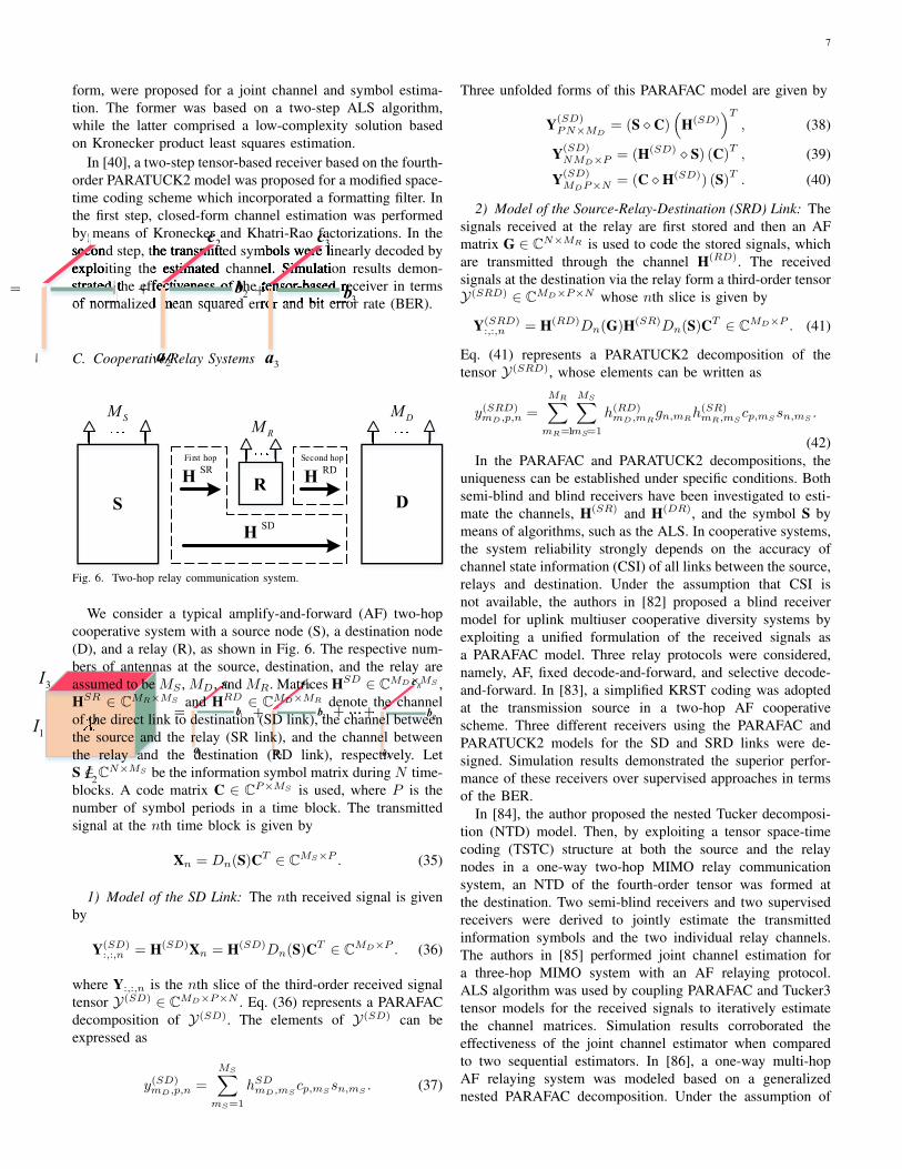
C. Cooperative/Relay Systems

a

b

c

second step, the transmitted symbols were linearly decoded byexploiting the estimated channel. Simulation results demon-strated the effectiveness of the tensor-based receiver in termsstrated the effectiveness of the tensor-based receiver in termsof normalized mean squared error and bit error rate (BER).strated the effectiveness of the tensor-based receiver in terms

1a

1b

1c

+

by means of Kronecker and Khatri-Rao factorizations. In thesecond step, the transmitted symbols were linearly decoded byexploiting the estimated channel. Simulation results demon-strated the effectiveness of the tensor-based receiver in termsof normalized mean squared error and bit error rate (BER).

C. Cooperative/Relay Systems

strated the effectiveness of the tensor-based receiver in termsstrated the effectiveness of the tensor-based receiver in termsof normalized mean squared error and bit error rate (BER).strated the effectiveness of the tensor-based receiver in termsof normalized mean squared error and bit error rate (BER).strated the effectiveness of the tensor-based receiver in terms

2c

2b

2a

+

second step, the transmitted symbols were linearly decoded byexploiting the estimated channel. Simulation results demon-strated the effectiveness of the tensor-based receiver in termsof normalized mean squared error and bit error rate (BER).

+strated the effectiveness of the tensor-based receiver in terms+strated the effectiveness of the tensor-based receiver in terms+strated the effectiveness of the tensor-based receiver in termsstrated the effectiveness of the tensor-based receiver in termsof normalized mean squared error and bit error rate (BER).strated the effectiveness of the tensor-based receiver in termsof normalized mean squared error and bit error rate (BER).strated the effectiveness of the tensor-based receiver in terms

3b

3a

3c

=

=1I

2I

3I

A1I

1J

1J

2J

3J

B2I2J

C

3J

3I

+

1a

1I

2I

3I

= +

2a 3a

1b 2b 3b

1c 2c 3c

,1ns,2ns

,n Rs

S W

OFDMOFDM

OFDM

12

M


Precodingmatrix

Antenna allocation

SMRM DM

SR

D


SDH

+

1a1I

2I

3I

= +++

2a Ra

1b 2b Rb

1c 2c Rc

+ ...

Fig. 6. Two-hop relay communication system.

We consider a typical amplify-and-forward (AF) two-hopcooperative system with a source node (S), a destination node(D), and a relay (R), as shown in Fig. 6. The respective num-bers of antennas at the source, destination, and the relay areassumed to be MS , MD, and MR. Matrices HSD ∈ CMD×MS ,HSR ∈ CMR×MS and HRD ∈ CMD×MR denote the channelof the direct link to destination (SD link), the channel betweenthe source and the relay (SR link), and the channel betweenthe relay and the destination (RD link), respectively. LetS ∈ CN×MS be the information symbol matrix during N time-blocks. A code matrix C ∈ CP×MS is used, where P is thenumber of symbol periods in a time block. The transmittedsignal at the nth time block is given by

Xn = Dn(S)CT ∈ CMS×P . (35)

1) Model of the SD Link: The nth received signal is givenby

Y(SD):,:,n = H(SD)Xn = H(SD)Dn(S)CT ∈ CMD×P . (36)

where Y:,:,n is the nth slice of the third-order received signaltensor Y(SD) ∈ CMD×P×N . Eq. (36) represents a PARAFACdecomposition of Y(SD). The elements of Y(SD) can beexpressed as

y(SD)mD,p,n =

MS∑mS=1

hSDmD,mS

cp,mSsn,mS

. (37)

Three unfolded forms of this PARAFAC model are given by

Y(SD)PN×MD

= (S C)(

H(SD))T

, (38)

Y(SD)NMD×P = (H(SD) S) (C)

T, (39)

Y(SD)MDP×N = (C H(SD)) (S)T . (40)

2) Model of the Source-Relay-Destination (SRD) Link: Thesignals received at the relay are first stored and then an AFmatrix G ∈ CN×MR is used to code the stored signals, whichare transmitted through the channel H(RD). The receivedsignals at the destination via the relay form a third-order tensorY(SRD) ∈ CMD×P×N whose nth slice is given by

Y(SRD):,:,n = H(RD)Dn(G)H(SR)Dn(S)CT ∈ CMD×P . (41)

Eq. (41) represents a PARATUCK2 decomposition of thetensor Y(SRD), whose elements can be written as

y(SRD)mD,p,n =

MR∑mR=1

MS∑mS=1

h(RD)mD,mR

gn,mRh(SR)mR,mS

cp,mSsn,mS

.

(42)In the PARAFAC and PARATUCK2 decompositions, the

uniqueness can be established under specific conditions. Bothsemi-blind and blind receivers have been investigated to esti-mate the channels, H(SR) and H(DR), and the symbol S bymeans of algorithms, such as the ALS. In cooperative systems,the system reliability strongly depends on the accuracy ofchannel state information (CSI) of all links between the source,relays and destination. Under the assumption that CSI isnot available, the authors in [82] proposed a blind receivermodel for uplink multiuser cooperative diversity systems byexploiting a unified formulation of the received signals asa PARAFAC model. Three relay protocols were considered,namely, AF, fixed decode-and-forward, and selective decode-and-forward. In [83], a simplified KRST coding was adoptedat the transmission source in a two-hop AF cooperativescheme. Three different receivers using the PARAFAC andPARATUCK2 models for the SD and SRD links were de-signed. Simulation results demonstrated the superior perfor-mance of these receivers over supervised approaches in termsof the BER.

In [84], the author proposed the nested Tucker decomposi-tion (NTD) model. Then, by exploiting a tensor space-timecoding (TSTC) structure at both the source and the relaynodes in a one-way two-hop MIMO relay communicationsystem, an NTD of the fourth-order tensor was formed atthe destination. Two semi-blind receivers and two supervisedreceivers were derived to jointly estimate the transmittedinformation symbols and the two individual relay channels.The authors in [85] performed joint channel estimation fora three-hop MIMO system with an AF relaying protocol.ALS algorithm was used by coupling PARAFAC and Tucker3tensor models for the received signals to iteratively estimatethe channel matrices. Simulation results corroborated theeffectiveness of the joint channel estimator when comparedto two sequential estimators. In [86], a one-way multi-hopAF relaying system was modeled based on a generalizednested PARAFAC decomposition. Under the assumption of

8

KRST coding implemented at each relay, a sequential closed-form semi-blind receiver was designed, wherein the informa-tion symbols and the individual channels were jointly esti-mated. For OFDM-based cooperative communication systems,a tensor-based blind signal recovery scheme was devised in[87]. The received multi-carrier signals were modeled as a 3-D tensor and a PARAFAC decomposition-based blind receiveralgorithm was employed for data detection. The work in [88]proposed two ST coding schemes, MKRST and MKronST,for multiple-antenna one-way two-hop MIMO relay system.These coding schemes generalize the standard Khatri-Raocoding by introducing extra space/time diversities. Parallelnon-iterative decoding methods are proposed for estimatingthe symbol matrix. In [89], the authors considered the multi-relaying systems, two tensor-based receivers were proposedto jointly estimate the channels and symbols in a semi-blindfashion. By exploiting the structure of the received signals, theauthors shown that the data for the relay-assisted link after STdecoding has a Kronecker structure, which can be recast as arank-one tensor based on PARAFAC analysis. The simulationresults also shown that the proposed receiver design has goodperformance-complexity trade-off.

D. Time-varying Channel Modeling

Tensor decompositions were considered for on-line appli-cations in [90], where the data were assumed to be seri-ally acquired and/or the underlying model was consideredto change frequently, resulting in a time-varying wirelesscommunication system. Given the PARAFAC decompositionof a tensor at instant t, two adaptive low-complexity algorithmswere provided to obtain the decomposition at instant t + 1by appending a new slice in the time dimension, and theirexcellent tracking capability was validated through simulation.

Doppler shifts in a time-varying mmWave scenario wereconsidered in [91]. The channel was assumed to have block-sparse and low-rank characteristics, since the change in anglewas much slower than that in path gain. By exploiting thesecharacteristics, a two-stage method was proposed. In the firststage, Block Orthogonal matching pursuit (BOMP) algorithmwas used to estimate the angles-of-arrival (AoAs)/angles-of-departure (AoDs). Based on the angle estimates, PARAFACdecomposition was used to estimate the Doppler shifts andpath gains in the second stage. Furthermore, the proposedalgorithm was shown to be close to the Cramer-Rao LowerBound (CRLB). For downlink multiuser-MIMO (MU-MIMO)communications over a time-varying channel, a transmissionframe structure was proposed in [92], wherein the angle andthe channel gain were to be estimated. By leveraging the sparsenature of mmWave channels, an adaptive angle estimationalgorithm was devised. The angle estimates were used todesign pilot beamforming for estimating the path gains. For thesame assumption of slower variations in angle than path gains,the authors in [93] proposed a two-stage tensor decompositionbased method for a single receiver. Doppler shift estimationwas achieved based on the estimated angles.

E. mmWave Communication System

Millimeter wave channels have a sparse scattering nature,leading to their low-rank structures and spread in the form ofclusters of paths over the angular domains, including the AoA,AoD, and elevation. This joint sparse and low-rank structurerenders the application of tensor models suitable in mmWavecommunication systems.

Consider a point-to-point uplink mmWave MIMO system,which comprises N antennas at the BS and M antennas at theMS. Beamforming techniques are implemented due to shortwavelength and severe path loss in mmWave communicationsystem. Analog beamforming is used in both BS and MS withone radio-frequency chain. At time instant t, the symbol s(t) istransmitted through an analog beamforming vector f(t) ∈ CN .The receiver combines the signals with receive beamformingvector w(t) ∈ CM . The combined signal at the receiver canbe expressed as

y(t) = wH(t)Hf(t)s(t) + wH(t)n(t) ∀t = 1, ..., T, (43)

where H ∈ CM×N is the channel matrix and n(t) denotesadditive Gaussian noise. For mmWave operation, the channelis usually characterized by a geometric model [91]

H =

L∑l=1

αlaBS(θl)aHMS(ψl), (44)

where L is the number of paths, αl is the complex gainassociated with the lth path, and θl and ψl are the AoA andAoD, respectively. The vectors aBS and aMS represent thearray response vectors and are given by

aBS(θl)=1√N

[1,ej

2πλ d sin(θl), ..., ej(N−1)

2πλ d sin(θl)

]T,

(45)

aMS(ψl)=1√M

[1,ej

2πλ d sin(ψl), ..., ej(N−1)

2πλ d sin(ψl)

]T.

(46)

The channel matrix can be further formulated as

H = ABSHvAHMS (47)

where ABS , [aBS(φ1), ..., aBS(φN1)] ∈ CN×N1 is theovercomplete dictionary matrix consisting of the BS steeringvectors corresponding to N1 discretized arrival angles. Like-wise, AMS ∈ CM×N2 can be obtained using MS steeringvectors corresponding to N2 discretized departure angles. Thematrix Hv ∈ CN1×N2 is sparse, with L non-zero entriescorresponding to the channel path gains, αl. By exploitingthe Kronecker product property of (4), the received signal canbe rewritten as

y(t) = wH(t)ABSHvAHMSf(t)s(t) + n′(t)

=[(AHMSf(t))T ⊗ (wH(t)ABS)

]h + n′(t)

= (fT (t)⊗ wH(t))(A∗MS ⊗ ABS)h + n′(t) (48)

9

where h , vec(Hv) and n′(t) is the equivalent noise. Collect-ing the received signals as y , [y(1), ..., y(T )]

T , we have

y =

fT (1)⊗ wH(1)...

fT (T )⊗ wH(T )

(A∗MS ⊗ ABS)h + n

, Ψh + n. (49)

The above model together with the unique characteristicsof mmWave time-varying channels can be exploited to esti-mate AoAs/AoDs. For example, the work in [94] consideredthe channel estimation problem for multi-user uplink MIMOmmWave communication systems, where both the BS and theusers were assumed to have hybrid beamforming structures.The low-rank structure of the received data was exploitedwithin a PARAFAC model and a layered pilot transmissionscheme was devised to reduce the training overhead. Theconditions to ensure the uniqueness of the decomposition wereused for the beamformer design. Similar to [94], the author in[95] considered the problem of downlink channel estimationfor mmWave MIMO-OFDM systems. The authors proposeda PARAFAC decomposition-based method for channel pa-rameter estimation, including angles, time delays, and fadingcoefficients. The analysis revealed that the uniqueness of theCPD could be guaranteed with a small training overhead. TheCRLB was also developed as a benchmark for the proposedtensor based algorithm.

The work in [96] combined dual-polarized (DP) antennaarrays with the double directional (DD) channel model fordownlink channel estimation. The combination was modeledas a low-rank four-way tensor and tensor decompositionalgorithms were used to effectively estimate the associatedchannel parameters. Furthermore, the DD channel with DParrays was shown to be identifiable under very mild conditions.In [97], a compressed tensor decomposition algorithm isadded to alleviate the training overhead. In [98], the practicalhardware impairment, i.e., carrier frequency offset (CFO) wasconsidered. The authors proposed a joint CFO and channelestimation method based on tensor modeling and compressedsensing which was proved to be more robust to a small numberof channel measurements via simulations. The work in [99]discussed the channel estimation problem under a MIMO-OFDM transmission assumption. A tensor-based minimummean square error (MMSE) channel estimator was proposedand then by incorporating a 3D sparse representation intothe tensor-based channel model, a tensor compressive sensing(tensor-CS) model is formulated by assuming that the channelis compressively sampled in space (radio-frequency chains),time (symbol periods), and frequency (pilot subcarriers),which is used as the basis for the formulation of a tensor-orthogonal matching-pursuit (T-OMP) estimator. The work[100] addressed the problem of joint downlink (DL) and uplink(UL) channel estimation for millimeter wave mmWave MIMOsystems using a tensor modeling approach. Assuming a closed-loop and multifrequency-based channel training framework,the algorithms developed therein jointly estimated both theDL and UL channels by concentrating most of the processingburden for channel estimation at the BS side.

F. BTD for Intersymbol Interference Problem

Consider the DS-CDMA model in (27). Let zmln denote thelth chip of the nth symbol of the mth user signal. If there isno ISI, then zmln = cm(l)sm(n). In this case, as in (27), thebaseband output for symbol n and chip l from the kth antenna

is xk,n,l =M∑m=1

hm(k)zmln. On the other hand, if the ISI exists

such that it has an impact over at most R symbols, then wehave

zmln =R∑r=0

Em(l, r)sm(n− r), (50)

where Em(l, r) denotes the overall impulse response of thelth chip and the most recent rth symbol. In this case, we canexpress xk,n,l in tensorial form as

X =M∑m=1

hm (EmSm), (51)

where Em ∈ RL×R and Sm ∈ RR×N is a Toeplitz matrixwith sm(n− r) as its (r, n)th element. Eq. (51) admits BTDin rank-(1, R,R) terms. Details of the corresponding essentialuniqueness condition and blind deconvolution algorithm canbe found in [69], [101].

Recently, coupled tensor decompositions have emerged asan important tool for handling missing data in signal pro-cessing and analysis of coupled data sets. The necessary andsufficient uniqueness conditions for coupled decompositionsdepend on the observed data sampling patterns. For example,the uniqueness conditions and linear algebra based algorithmsof coupled CPD and coupled BTD were both considered in[102], [103], where multi-coupled subtensors were formedwith partly observed data in the first two dimensions andfully observed data in the third dimension. The coupled tensordecompositions can be summarized as follows.

minfactors

Loss(subtensors, factors)+penalty(factors)

subject to constraints(factors)

IV. APPLICATIONS IN MIMO RADAR

The higher dimensional signal structures inherent in MIMOradar invite tensor-based signal processing solutions to the tar-get parameter estimation and transmit beamforming problems.The use of tensor models and milti-linear algebraic methodsin MIMO radar is not yet at the same level of maturity asin wireless communications, but some interesting results areexisting. Below, we give an overview of tensor-based methodsin bistatic and monostatic MIMO radar systems.

A. Tensor Techniques for Target Parameter Estimation inMIMO Radar

For a bistatic MIMO radar with an M -element transmitarray and an N -element receive array, the received signalmodel under the assumption of orthogonal transmit waveformsand a coherent processing interval (CPI) containing Q pulsescan be expressed as [56], [57]

Y = (A B)CT + Z, (52)

10

where Y ∈ CMN×Q contains the received data after matchedfiltering, Z is the spatially and temporally white additivenoise, CT ∈ CP×Q contains the reflection coefficients ofP targets corresponding to Q pulses, and A ∈ CM×P andB ∈ CN×P denote the respective steering matrices for trans-mit and receive arrays. Arranging the matched-filter outputsas a tensor Y ∈ CM×N×Q and following the definitions ofthe matrix unfoldings in Section II-B2, it can be observed thatmodel (52) represents the PARAFAC decomposition. As such,target parameter estimation can proceed within the PARAFACframework.

The target AoAs and AoDs were estimated using thePARAFAC model in [56] under narrowband far-field as-sumptions. The pth column of matrix A (matrix B) in (52)captures the delays across the different transmit (receive)antennas relative to a reference transmit (receive) antenna fora plane wavefront departing in (arriving from) the directionof the pth target. Two different models for target radar cross-section (RCS) fluctuations were considered. Swerling I modelassumes the RCS coefficients to be constant over the CPI,whereas in the Swerling II model, the RCS coefficients varyindependently from pulse to pulse. Conditions for essentialuniqueness guarantees were established which yielded usefulbounds on the number of resolvable targets.

The works in [57], [58], on the other hand, proposed tensor-based near-field localization algorithms for targets locatedcloser to the transmit and/or receive arrays of a bistatic MIMOradar. In this case, the pth column of matrix A (matrix B) wasdefined in terms of the exact path differences under sphericalwavefronts between the reference transmit (receive) antennaand other antennas in the transmit (receive) array for the pthtarget. The estimated target parameters included the AoAs,the AoDs, and the target distances from transmit and receivereference antennas. In [58], the parameters were obtainedthrough iteratively optimizing a least-squares cost functiondefined with respect to the elements of A and B. Alternatively,the authors in [57] first estimated A and B as factor matricesin an approximate low rank CPD of the tensor Y , which werethen used to estimate the target parameters by solving systemsof linear equations.

We note that the model in (52) as well as the afore-mentioned methods do not take into account the effects ofarray mutual coupling (MC) on target parameter estimation.MC however occurs in practice and can lead to perfor-mance degradation if not properly compensated. Both higher-order singular value decomposition (HOSVD) and PARAFACdecomposition-based methods have been recently proposed foraccurate target localization using MIMO radar in the presenceof mutual coupling [59], [104], [105].

A tensor-based sub-Nyquist monostatic MIMO radar wasproposed in [106] which used undersampled measurementsin spectral, spatial, Doppler, and temporal domains to jointlyestimate target AoAs, range, and Doppler. The received sig-nals were modeled as a partial third-order tensor. On-gridtarget parameters were estimated by solving a sparse recoveryproblem using tensor orthogonal matching pursuit, whereasa nuclear-norm regularized tensor completion method wasemployed for off-grid target parameters. The lower bounds on

the total numbers of antenna channels, transceiver frequencies,and pulses required for perfect recovery of both on-grid andoff-grid targets were also determined.

B. Transmit Array Interpolation in MIMO Radar

Together with waveform design, transmit beamspace (TB)design [107]–[110] is one of the fundamental problems inMIMO radar with colocated antennas. While designing TB,certain properties such as rotational invariance property (RIP)at the receive array can be ensured via TB matrix at thetransmit array for a monostatic MIMO radar [60]. It is es-pecially useful for reducing significantly the complexity ofsolving the target localization problem (e.g., AoA estimation– azimuth and elevation for two-dimensional (2-D) arrays) atthe receive array. If the RIP is ensured between more thantwo virtual subarrays (the solution for two subarrays related toeach other through RIP is the classical ESPRIT), the receivedsignals in MIMO radar can be arranged in a tensor and tensoralgebra then becomes the main tool for designing localizationalgorithms.

For example, consider a mono-static MIMO radar andassume that the transmit and receive arrays are placed on aplane and have arbitrary geometries. The receive array consistsof antenna elements randomly selected from the transmit array.Let the transmit antenna elements be located at the positionpm , [xm, ym]T ,m = 1, 2, . . . ,M . Then the M × 1 steeringvector of the transmit array can be expressed as

a(θ, φ) , [e−j2πuT (θ,φ)p1 , . . . , e−j2πu

T (θ,φ)pM ]T (53)

where u(θ, φ) , [sin θ cosφ, sin θ sinφ]T represents thepropagation vector, and θ, φ are the elevation and azimuth,respectively. Similarly, the steering vector of the receive arraycan be then expressed as

b(θ, φ) , [e−j2πuT (θ,φ)p1 , . . . , e−j2πu

T (θ,φ)pN ]T . (54)

Let sm(t) be the complex envelope of the mth transmitsignal where t represents the fast time, and then sm(t)Mm=1

be a set of M waveforms. Each waveform sm(t) has unitenergy, and all waveforms are orthogonal to each other duringone pulse, i.e.,

∫Tsm(t)s∗m′(t)dt = δ(m − m′), where T is

the radar pulse duration, δ(·) denotes the Dirac delta function,and L is the number of samples per pulse period. The signalradiated towards a spatial region of interest is therefore givenby

ζ(t, θ, φ) = aT (θ, φ)s(t) =M∑m=1

am(θ, φ)sm(t) (55)

where s(t) , [s1(t), . . . , sM (t)]T and am(θ, φ) is the mthelement of a(θ, φ).

Assuming that radar cross section (RCS) coefficients obeySwerling II model, for the case of K targets located in a spatialsector of interest, the received MIMO observation vector canbe expressed as

x(t, q) =K∑k=1

βk(q)(aT (θk, φk)s(t))b(θk, φk)+n(t, q) (56)

11

where q represent the slow time index, βk(q) is the RCScoefficient of kth target with variance σ2

β , and n(t, q) is thenoise vector modeled as complex spatial and temporal whiteGaussian process. Using the orthogonality property of thetransmit waveforms, the received data vector correspondingto the mth waveform after matched-filtering can be obtainedas

ym(q) =K∑k=1

(am(θk, φk)b(θk, φk)

)βk(q) + z(q) (57)

where ym(q) ∈ CN×1, z(q) is the noise vector after matched-filtering whose covariance matrix is given by σ2

nIN . Hence,the whole receive vector, i.e., the vector that is obtained bystacking ym(q), m = 1, . . . ,M , one under another, can bewritten as

y(q) = (A(θ, φ) B(θ, φ))β(q) + z(q) (58)

where A(θ, φ) , [a(θ1, φ1), . . . ,a(θK , φK)] is the transmitsteering matrix, B(θ, φ) , [b(θ1, φ1), . . . , b(θK , φK)] is thereceive steering matrix, and β(q) , [β1(q), . . . , βK(q)]T isthe vector of RCS coefficients during qth pulse.

Using the TB matrix at the transmitter, the received signalin qth pulse is given as

y(q) = B(θ, φ)Σ(q)AH(θ, φ)Ws(t) + z(q) (59)

where Σ(q) = diag(β(q)) and W is the TB matrix. Consid-ering Q pulses, the received 2D TB MIMO radar signal matrixY ∈ CMN×Q can be formed. Here M is the dimension ofthe transmit signal after TB transform. Then the corresponding2D TB MIMO radar tensor model can be expressed as

Y = A×R P + Z (60)

where steering tensor A is composed by stacking K targets’steering tensor Ak together, P , [β(1),β(2), . . . ,β(Q)]contains K vectors of targets’ RCS coefficients for Q pulses,and Z stands of the noise samples, which is assumed to beGaussian with zero mean, and R represents the Rth modetensor-matrix product.

Note that transmit and receive array geometries are arbitraryhere, and do not need to be uniform. Then TB also performsthe function of array interpolation as shown in [111]–[116],where the problem of the 2D transmit array interpolation andbeamspace design for mono-static MIMO radar with applica-tion to elevation and azimuth estimation has been addressed.The 2D transmit array interpolation has been formulated, forexample, as the minimax convex optimization problem withconstraints on array interpolation errors within a spatial sectorof interest while minimizing the transmit power outside thesector. The desired structure of the virtual transmit array(for example, L-shaped array) is then enforced. It allows tobenefit from translational invariance property when estimatingelevation and azimuth parameter at the receiver. The advantageof the high-dimensional structure inherent in the receivedsignal as explained above (the signal has been folded into ahigher-order tensor) allows for the use tensor-based ESPRITmethods.

C. Tensor Techniques for Parameter Estimation in MIMORadar with Arrays of Regular Geometries

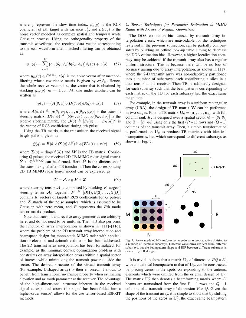
The DOA estimation bias caused by transmit array in-terpolation errors, which are unavoidable for the techniquesreviewed in the previous subsection, can be partially compen-sated by building an offline look-up table aiming to decreasethe DOA estimation bias. However, a higher localization accu-racy may be achieved if the transmit array also has a regularuniform structure. This is because there will be no loss ofaccuracy arising due to array interpolation, as shown in [117]where the 2-D transmit array was non-adaptively partitionedinto a number of subarrays, each contributing a slice in adata tensor at the receiver. Then TB is adaptively designedfor each subarray such that the beampatterns corresponding toeach matrix of the TB for each subarray had the exact samemagnitude.

For example, in the transmit array is a uniform rectangulararray (URA), the design of TB matrix W can be performedin two stages. First, a TB matrix U0 = [u1, . . . ,uk], with fullcolumn rank K, is designed over a spatial sector Θ = [θ1 θ2]and Φ = [φ1 φ2] using only the first (P −1) rows and (Q−1)columns of the transmit array. Then, a simple transformationis performed on U0 to produce TB matrices with identicalbeampatterns, but which correspond to different subarrays asshown in Fig. 7.

Fig. 7. An example of 2-D uniform rectangular array non-adaptive division toa number of identical subarrays. Different waveforms are sent from differentsubarrays, but the beampattern shape and RIP between different subarrays isensured by TB design.

It is trivial to show that a matrix U′0 of dimension PQ×K,with an identical beampattern to that of U0, can be constructedby placing zeros in the spots corresponding to the antennaelements which were omitted from the original design of U0.The matrix U′0 then denotes a beamforming matrix where Kbeams are transmitted from the first P − 1 rows and Q − 1columns of a transmit array of dimension P × Q. Given theshape of the transmit array, it is simple to show that by shiftingthe positions of the zeros in U′0, the exact same beampattern

12

can be achieved by subarrays containing the first P − 1 rowsand last Q−1 columns, the last P −1 rows and the first Q−1columns, and finally the last P − 1 and last Q − 1 columnsof the transmit array. These three matrices are denoted as U′1,U′2, and U′3, respectively. With these matrices defined, it iseasy to show that the following is true

aH(θ, φ)U′0 = ej2πdx sin θ cosφ(aH(θ, φ)U′1

)(61)

= ej2πdy sin θ sinφ(aH(θ, φ)U′2

)= ej2π(dx sin θ cosφ+dy sin θ sinφ)

(aH(θ, φ)U′3

).

The beamforming matrix W is then defined as W ,[U′0,U

′1,U

′2,U

′3] with an overall dimension of PQ × 4K.

Clearly, in the original design problem, the number of resolv-able targets K must be no larger than PQ/4.

Given the structure (61) imposed on the beamspace matrixW, let us turn our attention to (59). Rewriting the noiselessmatrix before vectorization allows to illustrate the structure ofW on DOA estimation. Specifically, we can write that

B(θ, φ)Σ(q)AH(θ, φ)W = B(θ, φ)Γ (62)

where Γ , Σ(q)AH(θ, φ)W. The matrix Γ is the source sig-nal matrix, and has dimension L×4K. Let Γ0 = Σ(τ)AHU′0is the source signal matrix corresponding to K beams elim-inated from the first (P − 1) rows and (Q − 1) columns ofthe transmit array. Using the relations (61), we define matricesΩi, i ∈ 0, 1, 2, 3 as the L×L diagonal matrices with the l-thdiagonal entry of Ωi being the complex exponential in (61)which relates aH(θ, φ)U′0 to aH(θ, φ)U′i. The matrix Ω0 isobviously the identity matrix. Then (62) can be expressed asthe following block partitioned matrix

BΓ = B

[Ω0Γ0 Ω1Γ0 Ω2Γ0 Ω3Γ0

](63)

=

[BΩ0 BΩ1 · · · BΩ3

]bdiag4(Γ0)

where we drop the dependence of B on (θ, φ) and bdiagm(·)takes a single matrix as an argument, and creates a blockdiagonal matrix whose m blocks are equal to its argument.The matrix BΩ0 is simply the receiver response matrix to Ktargets. The virtual receiver response matrices BΩ1, BΩ2, andBΩ3 are exactly the receiver response matrices to K targets,for identical receive arrays that are linearly displaced from ouractual receiver by [dx, 0], [0, dy], and [dx, dy], respectively.The source signal matrix Γ0 is a common factor for each.From (63) it is visible that the structure for W enforces analgebraic structure on Y which can be exploited by search-freealgorithms for DOA estimation, such as, for example, ESPRIT.Moreover, (63) can be viewed as an unfolding of a tensor witheach slice to be one of the 4 matrices BΩi i = 0, 1, 2, 3.

Matrix Y has dimension 4RK × Q and it obtained byunfolding the corresponding tensor Y of signal for all Qpulses. After defining the matrix selection operator Fi(·)which selects the (iM/4 + 1)–M/4(i + 1) rows from an

arbitrary matrix with M rows, where i = 0, 1, 2, 3, Y anda new matrix Y′ can be expressed as

Y =

F0(Y)F1(Y)F2(Y)F3(Y)

, Y′ =

F0(Y)F2(Y)F1(Y)F3(Y)

. (64)

Forming the cross correlation matrices RY = I−1YYH andRY′ = I−1Y′Y′H , and performing ESPRIT on both willyield a vector of L phase arguments which are directly propor-tional to ζl and γl. Defining a complex number zl = γl+jζl theangle estimates are given by φl = arctan(ζl/γl), and θl = |zl|.

The above described structure of the TB matrix W is justa special case shown in Fig. 7. However, the approach can begeneralized to allow for a flexible subarray selection, allow formore general that just URA transmit array geometries, allowfor more computationally efficient tensor decomposition tech-niques that use the additional structures in the signal tensor.These and other generalizations have been addressed in therecent work [118]. The additional structure in the signal tensorcomes from the Vandermonde structure of the factor matrices.The term that was recently coined for decomposition methodsof tensors with some additional structures that need to betaken into account and may lead to significant improvement ofcomputational efficiency is constrained factor decomposition[27]. The decomposition methods proposed in [118] belongsthen to this class of tensor decomposition techniques.

Finally, an extension of TB design method for AoA/AoDestimation in bistatic MIMO radar has been recently proposedin [119], wherein uniform power distribution across the trans-mit array elements was achieved via inequality constraints.

D. Tensor Techniques for Slow-Time MIMO Radar

A notifiable disadvantage of MIMO radar is the needof multiple orthogonal waveforms. Indeed, multi-waveformMIMO radar demands several signal generators to transmitorthogonal waveforms, which can be costly and unacceptablefor especially in such applications as automotive MIMO radar.However, using additionally M phase shifters at the transmitarray incited of a multiple orthogonal waveform generator,the implementation of MIMO radar can be still upgradedeasily from a legacy SIMO radar, where only one signalgenerator is used. The associated waveform design approachhas been called Doppler division multiple access (DDMA)technique, and the signal model for this techniques can alsobe represented in tensor form [120]. Such approach is calledslow-time MIMO radar, and its essence is to modulate eachtransmit signal with a unique Doppler shift via a pulse-to-pulsephase coding. Under this circumstance, the model in (52) canbe modified to represent the received signal of MIMO radarusing DDMA technique as

Y =[(A B) CT

]D + Z (65)

where D , (IM 1N×M ) P, P ∈ CM×Q is the phase mod-ulation matrix that achieves waveform diversity in Dopplerdomain, 1N×M is a N ×M all-one matrix, and the symbol denotes the Hadamard (element-wise) product. It can be

13

observed that matrix D also represents the parallel factor(PARAFAC) decomposition. It is worth noting that the inde-pendence of phase modulation matrix and the received signalcan be exploited in the context of slow-time MIMO radar.Based on this property, a novel tensor model was designed toimprove the target parameter estimation performance is [120].Moreover, the additional phases on transmit array lead to acyclically varying transmit beampattern from pulse to pulse,which can be regarded as a special case of TB design.

V. CONCLUSION

In this paper, we presented a comprehensive overview oftensor decompositions in wireless communications and MIMOradar. We provided a description of basic tensor operationsand tensor decompositions, thus establishing the preliminariesfor advanced application-driven discussions. Within the area ofwireless communications, we provided an in-depth descriptionof tensor-based methods for blind symbol recovery and chan-nel parameter estimation, focusing on CDMA, STF, cooper-ative/relay, MIMO, and mmWave systems. We also reviewedtensor techniques for transmit beamspace design and targetparameter estimation in MIMO radar. The presented methodsand strategies highlighted the prospects and potential of tensoralgebra and decompositions in wireless communications andMIMO radar.

REFERENCES

[1] A. Cichocki et al. (Mar. 2014). “Tensor decompositions for signalprocessing applications from two-way to multiway component analysis,”IEEE Signal Process Mag., vol. 32, no. 2, pp. 145–163, Mar. 2015, doi:10.1109/MSP.2013.2297439.

[2] G. Favier and A. A. L. F. de, “Overview of constrained PARAFACmodels,” EURASIP J. Adv. Signal Process., vol. 2014, no. 1, pp. 4–142,2014.

[3] N. D. Sidiropoulos, L. De Lathauwer, X. Fu, K. Huang, E. E. Papalex-akis and C. Faloutsos, “Tensor Decomposition for Signal Processing andMachine Learning,” IEEE Trans. Signal Process., vol. 65, no. 13, pp.3551–3582, 1 Jul. 2017, doi: 10.1109/TSP.2017.2690524.

[4] Y. Ji, Q. Wang, X. Li and J. Liu, “A Survey on Tensor Techniques andApplications in Machine Learning,” IEEE Access, vol. 7, pp. 162950–162990, 2019, doi: 10.1109/ACCESS.2019.2949814.

[5] A. L. F. de Almeida, G. Favier, J. P. C. L. da Costa, and J. C. M.Mota, “Overview of tensor decompositions with applications to com-munications,” in Signals and Images: Advances and Results in Speech,Estimation, Compression, Recognition, Filtering, and Processing, R.Coelho, V. Nascimento, R. de Queiroz, J. Romano, and C. Cavalcante,Eds. CRC-Press, Jan. 2016, no. Chapter 12, pp. 325–356.

[6] F. L. Hitchcock, “The expression of a tensor or a polyadic as a sum ofproducts,” J. Math. Phys., vol 6, pp. 164–189, 1927.

[7] F. L. Hitchcock, “Multilple invariants and generalized rank of a p-waymatrix or tensor,” J. Math. Phys., vol 7, pp. 39–79, 1927.

[8] L. R. Tucker, “Implications of factor analysis of three-way matricesfor measurement of change,” in Problems in Measuring Change, C. W.Harris, Ed., University of Wisconsin Press, 1963, pp. 122–137.

[9] L. R. Tucker, “The extension of factor analysis to three-dimensionalmatrices,” in Contributions to Mathematical Psychology, H. Gulliksenand N. Frederiksen, Eds., Holt, Rinehardt, & Winston, New York, NY,1964, pp. 110–127.

[10] L. R. Tucker, “Some mathematical notes on three-mode factor analysis,”Psychometrika, vol. 31, no. 3, pp. 279–311, 1966.

[11] J. D. Carroll and J. J. Chang, “Analysis of individual differencesin multidimensional scaling via an N-way generalization of “Eckart-Young” decomposition,” Psychometrika, vol. 35, no. 3, pp. 283–319,1970.

[12] R. A. Harshman, “Foundations of the PARAFAC procedure: Modelsand conditions for an “explanatory” multi-modal factor analysis,” UCLAWorking Papers in Phonetics, vol. 16, pp. 1–84, 1970.

[13] A. Smilde, R. Bro, and P. Geladi, Multi-Way Analysis: Applications inthe Chemical Sciences, Wiley, Hoboken, NJ, 2004.

[14] P. Kroonenberg, Applied Multiway Data Analysis, Wiley, Hoboken, NJ,2008.

[15] L. De Lathauwer, J. Castaing, and J.-F. Cardoso, “Fourth-order cumulantbased blind identification of underdetermined mixtures,” IEEE Trans.Signal Process., vol. 55, no. 6, pp. 2965–2973, 2007.

[16] L. De Lathauwer and A. de Baynast, “Blind deconvolution of DS-CDMAsignals by means of decomposition in rank-(1, L, L) terms,” IEEE Trans.Signal Process., vol. 56, no. 4, pp. 1562–1571, 2008.

[17] L. De Lathauwer and B. De Moor, “From matrix to tensor: Multilinearalgebra and signal processing,” in Mathematics in Signal Processing IV,J. McWhirter and I. Proudler, Eds., Clarendon Press, Oxford, UK, 1998,pp. 1–15.

[18] C. A. R. Fernandes, J. Du, A. P. da Silva, and A. L. F. de Almeida,“Applications of tensor models in wireless communications and mobilecomputing”, Wirel. Commun. Mob. Comput., pp. 7393080:1-393080:2,2020. doi: 10.1155/2020/7393080.

[19] A. J. Paulraj, D. A. Gore, R. U. Nabar, and H. Bolcskei, “An overviewof MIMO communications: A key to gigabit wireless,” Proc. IEEE, vol.92, no. 2, pp. 198–218, Feb. 2004.

[20] B. Hochwald, T. L. Marzetta, and C. B. Papadias, “A transmitter diversityscheme for wideband CDMA systems based on space-time spreading,”IEEE J. Sel. Areas Commun., vol. 19, no. 1, pp. 48–60, 2001.

[21] H. Huang, H. Viswanathan, and G. J. Foschini, “Multiple antennas in cel-lular CDMA systems: transmission, detection, and spectral efficiency,”IEEE Trans. Wireless Commun., vol. 1, no. 3, pp. 383–392, 2002.

[22] R. Doostnejad, T. J. Lim, and E. Sousa, “Space-time spreading codesfor a multiuser MIMO system,” in Proc. 36th Asilomar Conf. Signals,Syst. Comp., Pacific Grove, CA, Nov. 2002, pp. 1374–1378.

[23] N. D. Sidiropoulos,, G. B. Giannakis, and R. Bro, “Blind PARAFACreceivers for DS-CDMA systems,” IEEE Trans. Signal Process., vol.48, no. 3, pp. 810–823, 2000.

[24] Y. Rong, S.A. Vorobyov, A.B. Gershman, and N.D. Sidiropoulos, “Blindspatial signature estimation via time-varying user power loading andparallel factor analysis,” IEEE Trans. Signal Process., vol. 53, no. 5,pp. 1697–1710, 2005.

[25] A. L. F. de Almeida, G. Favier, and J. C. M. Mota, “PARAFAC-based unified tensor modeling for wireless communication systems withapplication to blind multiuser equalization,” Signal Process., vol. 87, no.2, pp. 337–351, 2007.

[26] N. D. Sidiropoulos and G. Z. Dimic, “Blind multiuser detection in W-CDMA systems with large delay spread,” IEEE Signal Process. Lett.,vol. 8, no. 3, pp. 87–89, 2001.

[27] A. L. F. de Almeida, G. Favier, and J. C. M. Mota, “A constrainedfactor decomposition with application to MIMO antenna systems,” IEEETrans. Signal Process., vol. 56, no. 6, pp. 2429–2442, Jun. 2008, doi:10.1109/TSP.2008.917026.

[28] A. L. F. de Almeida, G. Favier, and J. C. M. Mota, “Constrained tensormodeling approach to blind multiple-antenna CDMA schemes,” IEEETrans. Signal Process., vol. 56, no. 6, pp. 2417–2428, 2008.

[29] G. R. Stuber, J. R. Barry, S. W Mclaughlin, Y. Li, M. A. Ingram, and T.G. Pratt, “Broadband MIMO-OFDM wireless communications,” Proc.IEEE, vol. 92, no. 2, pp. 271–294, 2004.

[30] D. Agrawal, V. Tarokh, A. Naguib, and N. Seshadri, “Space-timecoded OFDM for high data-rate wireless communications over widebandchannels,” in Proc. Veh. Technol. Conf., Ottawa, Canada, 1998, pp. 2232–2236.

[31] H. Bolcskei and A. Paulraj, “Space-frequency coded broadband OFDMsystems,” in Proc. Wireless Commun. Netw. Conf., Chicago, IL, 2000,pp. 1–6.

[32] W. Su, Z. Safar, and K. J. R. Liu, “Full-rate full-diversity space-frequency codes with optimum coding advantage,” IEEE Trans. Inf.Theory, vol. 51, no. 1, pp. 229–249, 2005.

[33] W. Su, Z. Safar, and K. J. R. Liu, “Towards maximum achievablediversity in space, time and frequency: Performance analysis and codedesign,” IEEE Trans. Commun., vol. 4, no. 4, pp. 847–1857, 2005.

[34] N. D. Sidiropoulos and R. S. Budampati, “Khatri-Rao space-time codes,”IEEE Trans. Signal Process., vol. 50, no. 10, pp. 2396–2407, 2002.

[35] A. L. F. de Almeida, G. Favier, “Unified tensor model for space-frequency spreading-multiplexing (SFSM) MIMO communication sys-tems,” EURASIP J. Adv. Signal Process, vol. 2013, pp. 48, 2013.

[36] G. Favier, M. N. Costa, A. L. F. de Almeida, and J. M. T. Romano,“Tensor space-time (TST) coding for MIMO wireless communicationsystems,” Signal Process., vol. 92, no. 4, pp. 1079–1092, 2012.

14

[37] A. L. F. de Almeida, G. Favier, and J. C. M. Mota, “Space-timespreading-multiplexing for MIMO wireless communications systemsusing the PARATUCK-2 tensor model,” Signal Process., vol. 89, no.11, pp. 2103–2116, 2009.

[38] A. L. F. de Almeida, G. Favier, and L. R. Ximenes, “Space-time-frequency (STF) MIMO communication systems with blind receiverbased on a generalized PARATUCK2 model,” IEEE Trans. SignalProcess., vol. 61, no. 8, pp. 1895–1909, 2013.

[39] G. Favier and A. L. F. de Almeida, “Tensor space-time-frequency codingwith semi-blind receivers for MIMO wireless communication systems,”IEEE Trans. Signal Process., vol. 62, no. 22, pp. 5987–6002, 2014.

[40] G. T. de Araujo and A. L. F. de Almeida, “Closed-form channelestimation for MIMO space-time coded systems using a fourth-ordertensor-based receiver,” Circuits Syst. Signal Process., vol. 37, no. 3, pp.1343–1357, 2017.

[41] X. Han, A. L. F. de Almeida, and Z. Yang,“Channel estimation forMIMO multi-relay systems using a tensor approach,” EURASIP J.Advances in Signal Process., vol. 163, no. 1, 2014.

[42] Y. Rong, M. R. A. Khandaker, and Y. Xiang, “Channel estimation ofdual-hop MIMO. relay system via parallel factor analysis,” IEEE Trans.Wireless Commun., vol. 11, no. 6, pp. 2224–2233, 2012.

[43] L. R. Ximenes, G. Favier, and A. L. F. de Almeida, “Semi-blindreceivers for non-regenerative cooperative MIMO communications basedon nested PARAFAC modeling,” IEEE Trans. Signal Process., vol. 63,no. 18, pp. 4985–4998, 2015.

[44] J. Li and P. Stoica (Ed.), MIMO Radar Signal Processing, John Wiley& Sons, Hoboken, NJ, 2009.

[45] J. Bergin and J. R. Guerci, MIMO Radar: Theory and Application,Artech House, Boston, MA, 2018.

[46] K. W. Forsythe and D. W. Bliss, “MIMO radar waveform constraints forGMTI,” IEEE J. Sel. Topics Signal Process., vol. 4, no. 1, pp. 21–32,Feb. 2010

[47] P. Lombardo, D. Pastina and F. Turin, “Ground moving target detectionbased on MIMO SAR systems,” IEEE J. Sel. Topics Appl. Earth Observ.Remote Sens., vol. 8, no. 11, pp. 5081–5095, 2015.

[48] G. J. Frazer, “Experimental results for MIMO methods applied in over-the-horizon radar,” IEEE Aerosp. Electronic Syst. Mag., vol. 32, no. 12,pp. 52–69, 2017.

[49] J. Hu, M. Li, Q. He, Z. He and R. S. Blum, “Joint Estimation of MIMO-OTH Radar Measurements and Ionospheric Parameters,” IEEE Trans.Aerosp. Electronic Syst., vol. 53, no. 6, pp. 2789–2805, 2017.

[50] Y. I. Abramovich, G. J. Frazer and B. A. Johnson, “Principles of mode-selective MIMO OTHR,” IEEE Trans. Aerosp. Electronic Syst., vol. 49,no. 3, pp. 1839–1868, 2013.

[51] S. Sun, A. P. Petropulu and H. V. Poor, “MIMO radar for advanceddriver-assistance systems and autonomous driving: Advantages andchallenges,” IEEE Signal Process. Mag., vol. 37, no. 4, pp. 98–117,2020.

[52] S. Saponara, M. S. Greco and F. Gini, “Radar-on-chip/in-package inautonomous driving vehicles and intelligent transport systems: Oppor-tunities and challenges,” IEEE Signal Process. Mag., vol. 36, no. 5, pp.71–84, 2019.

[53] F. Liu, C. Masouros, A. P. Petropulu, H. Griffiths and L. Hanzo, “Jointradar and communication design: Applications, state-of-the-art, and theroad ahead,” IEEE Trans. Commun., vol. 68, no. 6, pp. 3834–3862, 2020.

[54] A. Hassanien, M. G. Amin, E. Aboutanios and B. Himed, “Dual-functionradar communication systems: A solution to the spectrum congestionproblem,” IEEE Signal Process. Mag., vol. 36, no. 5, pp. 115-126, 2019.

[55] A. Hassanien, M. G. Amin, Y. D. Zhang and F. Ahmad, ”Signalingstrategies for dual-function radar communications: an overview,” IEEEAerosp. Electronic Syst. Mag., vol. 31, no. 10, pp. 36-45, 2016.

[56] D. Nion and N. D. Sidiropoulos, “Tensor algebra and multidimensionalharmonic retrieval in signal processing for MIMO radar,” IEEE Trans.Signal Process., vol. 58, no. 11, pp. 5693–5705, 2010.

[57] I. Podkurkov and L. Hamidullina and E. Traikov and M. Haardt andA. Nadeev,“Tensor-based near-field localization in bistatic MIMO radarsystems,” in Proc. 22nd Int. ITG Workshop on Smart Antennas, Bochum,Germany, 2018, pp. 1–8.

[58] P. R. Singh and Y. Wang and P. Charge,“Bistatic MIMO radar for nearfield source localisation using PARAFAC,” Electronics Letters, vol. 52,no. 12, pp. 1060–1061, 2016.

[59] X. Wang and W. Wang and J. Liu and Q. Liu and B. Wang, “Tensor-based real-valued subspace approach for angle estimation in bistaticMIMO radar with unknown mutual coupling,” Signal Process., vol. 116,pp. 152–158, 2015.

[60] A. Khabbazibasmenj and A. Hassanien and S.A. Vorobyov andM. W. Morency, “Efficient transmit beamspace design for search-freebased DOA estimation in MIMO radar,” IEEE Trans. Signal Process.,vol. 62, no. 6, pp. 1490–1500, 2014.

[61] T.G. Kolda and B.W. Bader, “Tensor decompositions and applications,”Siam Review, vol. 51, no. 3, pp. 455–500, 2009.

[62] P. Comon, “Tensors : A brief introduction,” IEEE Signal Process. Mag.,vol. 31, no. 3, pp. 44–53, 2014.

[63] L. Grasedyck, D. Kressner, and C. Tobler, “A literature survey of lowrank tensor approximation techniques,” GAMM-Mitteilungen, vol. 36,no. 1, pp. 53–78, 2013.

[64] A. L. F. de Almeida. “Tensor modeling and signal processing forwireless communication systems,” Networking and Internet Architecture,Universite de Nice Sophia Antipolis, 2007.

[65] L. De Lathauwer, “Decompositions of a higher-order tensor in blockterms – Part II: Definitions and uniqueness,” SIAM J. Matrix Analysisand Applications, vol. 30, no. 3, pp. 1033–1066, 2008.

[66] L. De Lathauwer and D. Nion, “Decompositions of a higher-order tensorin block terms – Part III: Alternating least squares algorithms,” SIAM J.Matrix Analysis and Applications, vol. 30, no. 3, pp. 1067–1083, 2008.

[67] L. Sorber, M. Van Barel, and L. De Lathauwer, “Optimization-basedalgorithms for tensor decompositions: Canonical polyadic decomposi-tion, decomposition in rank-(l r,l r,1) terms, and a new generalization,”SIAM J. Optimization, vol. 23, no. 2, pp. 695–720, 2013.

[68] L. De Lathauwer, “Blind separation of exponential polynomials and thedecomposition of a tensor in rank-(l r,l r,1) terms,” SIAM J. MatrixAnalysis and Applications, vol. 32, no. 4, pp. 1451–1474, 2011.

[69] L. De Lathauwer, “Block component analysis, a new concept for blindsource separation,” in Int. Conf. Latent Variable Analysis and SignalSeparation, Springer, 2012, pp. 1–8.

[70] S. A Vorobyov, Y. Rong, N. D. Sidiropoulos, A. B. Gershman, “Robustiterative fitting of multilinear models,” IEEE Trans. Signal Processing,vol. 53, no. 8, pp. 2678–2689, 2005.

[71] E. E. Papalexakis, C. Faloutsos, N. D. Sidiropoulos, “Parcube: Sparseparallelizable tensor decompositions,” in Proc. Joint European Confer-ence on Machine Learning and Knowledge Discovery in Databases,Sept. 2012, pp. 521–536.

[72] A. P. Liavas, N. D. Sidiropoulos, “Parallel algorithms for constrainedtensor factorization via alternating direction method of multipliers,”IEEE Trans. Signal Processing, vol. 63, no. 20, pp. 5450–5463, 2015.

[73] M. Sørensen and L. De Lathauwer, “Coupled tensor decompositions forapplications in array signal processing,” in Proc. IEEE 5th Int. WorkshopComputational Advances in Multi-Sensor Adaptive Process., 2013, pp.228–231.

[74] G. Zhang, X. Fu, J. Wang, X.-L. Zhao, and M. Hong, “Spectrumcartography via coupled block-term tensor decomposition,” IEEE Trans.Signal Process., vol. 68, pp. 3660-3675, 2020.

[75] G. Zhang, X. Fu, K. Huang, and J. Wang, “Hyperspectral super-resolution: A coupled nonnegative block-term tensor decompositionapproach,” in Proc. IEEE 8th Int. Workshop Computational Advances inMulti-Sensor Adaptive Process., 2019, pp. 470–474.

[76] Y. Qi, P. Comon, and L. H. Lim, “Uniqueness of nonnegative tensorapproximations,” IEEE Trans. Inf. Theory, vol. 62, no. 4, pp. 2170–2183, 2016.

[77] N. D. Sidiropoulos and R. Bro. “On the uniqueness of multilineardecomposition of N-way arrays,” J. Chemometrics, vol. 14, pp. 229–239, 2000.

[78] L. Chiantini and G. Ottaviani, “On Generic Identifiability of 3-Tensorsof Small Rank,” SIAM J. Matrix Anal. Appl., vol. 33, no. 3, pp. 1018–1037, 2012.

[79] Harshman, R.A., Lundy, M.E. “Uniqueness proof for a family ofmodels sharing features of Tucker’s three-mode factor analysis andPARAFAC/candecomp.” Psychometrika, vol, 61, pp. 133–154, 1996.

[80] G. Favier, A.L.F. de Almeida, “Overview of constrained PARAFACmodels,” EURASIP J. Adv. Signal Process. 2014, 142 (2014).

[81] J. B. Kruskal, “Three-way arrays: Rank and uniqueness or trilinear de-compositions, with applications to arithmetic complexity and statistics,”Linear Algebra Appl., vol. 18, pp. 95–138, 1977.

[82] C. A. R. Fernandes, A. L. F. de Almeida, and D. B. da Costa, “Unifiedtensor modeling for blind receivers in multiuser uplink cooperativesystems,” IEEE Signal Process. Lett., vol. 19, no. 5, pp. 247–250, 2012.

[83] L. R. Ximenes, G. Favier, A. L. F. de Almeida, and Y. C. B. Silva,“PARAFAC-PARATUCK semi-blind receivers for two-hop cooperativeMIMO relay systems,” IEEE Trans. Signal Process., vol. 62, no. 14, pp.3604–3615, 2014.

15

[84] G. Favier, C. A. Fernandes, and A. L. F. de Almeida, “Nested Tuckertensor decomposition with application to MIMO relay systems usingtensor space-time coding (TSTC),” Signal Process., vol. 128, pp. 318–331, 2016.

[85] I. V. Cavalcante, A. L. F. de Almeida, and M. Haardt, “Joint channelestimation for three-hop MIMO relaying systems,” IEEE Signal Process.Lett., vol. 22, no. 12, pp. 2430–2434, 2015.

[86] W. C. Freitas, G. Favier, G., and A. L. F. de Almeida, “Sequentialclosed-form semi-blind receiver for space-time coded multi-hop relayingsystems,” IEEE Signal Process. Lett., vol. 24, no. 12, pp. 1773–1777,2017.

[87] Z. Wang, J. Wang, C. Xing, Z. Fei, and J. Kuang, “Tensor-based blindsignal recovery for multi-carrier amplify-and-forward relay networks,”Science China Information Sciences, vol. 57, no. 10, pp. 1–11, 2014.

[88] W. Freitas, G. Favier, A. L. F. de Almeida, “Generalized Khatri-Rao andKronecker space-time coding for MIMO relay systems with closed-formsemi-blind receivers,” Signal Process., vol.151, pp. 19–31, 2018.

[89] B. Sokal, A. L. F. de Almeida, M. Haardt, “Semi-blind receivers forMIMO multi-relaying systems via rank-one tensor approximations,”Signal Process., vol. 166, pp. 107–254, 2020.

[90] D. Nion and N. D. Sidiropoulos “Adaptive algorithms to track thePARAFAC decomposition of a third-order tensor,” IEEE Trans. SignalProcess, vol. 57, no. 6, pp. 2299–2310, 2009.

[91] L. Cheng, G. Yue, D. Yu, Y. Liang, and S. Li, “Millimeter wave time-varying channel estimation via exploiting block-sparse and low-rankstructures,” IEEE Access, vol. 7, pp. 123355–123366, 2019.

[92] Q. Qin, G. Lin, P. Cheng, and B. Gong, “Time-varying channel estima-tion for millimeter wave multiuser MIMO systems,” IEEE Trans. Veh.Technol., vol. 67, no. 10, pp. 9435–9448, 2018.

[93] L. Cheng, G. Yue, X. Xiong, Y. Liang and S. Li, “Tensor decomposition-aided time-varying channel estimation for millimeter wave MIMOsystems,” IEEE Wireless Commun. Lett., vol. 8, no. 4, pp. 1216–1219,2019.

[94] Z. Zhou, J. Fang, L. Yang, H. Li, Z. Chen, and S. Li, “Channelestimation for millimeter-wave multiuser MIMO systems via PARAFACdecomposition,” IEEE Trans. Wireless Commun., vol. 15, no. 11, pp.7501–7516, 2016.

[95] Z. Zhou, J. Fang, L. Yang, H. Li, Z. Chen and R. S. Blum, “Low-rank tensor decomposition-aided channel estimation for millimeter waveMIMO-OFDM systems,” IEEE J. Sel. Areas Commun., vol. 35, no. 7,pp. 1524–1538, 2017.

[96] C. Qian, X. Fu, N. D. Sidiropoulos, and Y. Yang, “Tensor basedparameter estimation of double directional massive MIMO channel withdual-polarized antennas,” in Proc. IEEE Int. Conf. Acoust., Speech,Signal Process., Calgary, Canada, 2018, pp. 3884–3888.

[97] C. Qian, X. Fu, N. D. Sidiropoulos, and Y. Yang, “Tensor-based channelestimation for dual-polarized massive MIMO systems,” IEEE Trans.Signal Process., vol. 66, no. 24, pp. 6390–6403, 2018.

[98] L. N. Ribeiro, A. L. F. de Almeida, N. J. Myers and R. W. Heath,“Tensor-based Estimation of mmWave MIMO Channels with CarrierFrequency Offset,” in Proc. ICASSP 2019, Brighton, United Kingdom,2019, pp. 4155–4159.

[99] D. C. Araujo, A. L. F. de Almeida, J. P. C. L. Da Costa and R. T. deSousa, “Tensor-Based Channel Estimation for Massive MIMO-OFDMSystems,” IEEE Access, vol. 7, pp. 42133–42147, 2019.

[100] P. R. B. Gomes, A.L. F. de Almeida, J. P. C. L. da Costa, R. T. de Sousa,“Joint DL and UL Channel Estimation for Millimeter Wave MIMOSystems Using Tensor Modeling”, Wirel. Commun. Mob. Comput., vol.2019, 2019.

[101] L. De Lathauwer and A. de Baynast, “Blind deconvolution of DS-CDMA signals by means of decomposition in rank-(1, l, l) terms,” IEEETrans. Signal Process., vol. 56, no. 4, pp. 1562–1571, 2008.

[102] M. Sørensen and L. D. De Lathauwer, “Coupled canonical polyadicdecompositions and (coupled) decompositions in multilinear rank-

[105] F. Wen and Z. Zhang and K. Wang and G. Sheng and G. Zhang, “Angleestimation and mutual coupling self-calibration for ULA-based bistaticMIMO radar,” Signal Process., vol. 144, no. Supplement C, pp. 61–67,2017.

(l r,n,l r,n,1) terms – Part I: Uniqueness,” SIAM J. Matrix Analysis andApplications, vol. 36, no. 2, pp. 496–522, 2015.

[103] M. Sørensen, I. Domanov, and L. De Lathauwer, “Coupled canonicalpolyadic decompositions and (coupled) decompositions in multilinearrank-(l r,n,l r,n,1) terms – Part II: Algorithms,” SIAM J. Matrix Analysisand Applications, vol. 36, no. 3, pp. 1015–1045, 2015.

[104] F. Wen and X. Xiong and Z. Zhang, “Angle and mutual couplingestimation in bistatic MIMO radar based on PARAFAC decomposition,”Digital Signal Process., vol. 65, pp. 1–10, 2017.

[106] S. Na, K. V. Mishra, Y. Liu, Y. C. Eldar and X. Wang, ”TenD-SuR: Tensor-Based 4D Sub-Nyquist Radar,” in IEEE Signal Pro-cessing Letters, vol. 26, no. 2, pp. 237-241, Feb. 2019, doi:10.1109/LSP.2018.2885617.

[107] A. Hassanien and S. A. Vorobyov, “Phased-MIMO radar: A tradeoffbetween phased-array and MIMO radars,” IEEE Trans. Signal Process.,vol. 58, no. 6, pp. 3137-3151, Jun. 2010.

[108] A. Hassanien and S. A. Vorobyov, “Transmit energy focusing for DOAestimation in MIMO radar with colocated antennas,” IEEE Trans. SignalProcess., vol. 59, no. 6, pp. 2669-2682, Jun. 2011.

[109] A. Khabbazibasmenj, S. A. Vorobyov, A. Hassanien, and M. W.Morency, “Transmit beamspace design for direction finding in colo-cated MIMO radar with arbitrary receive array and even number ofwaveforms,” in Proc. 46th Annual Asilomar Conf. Signals, Systems, andComputers, Pacific Grove, California, USA, pp. 1307-1311, Nov. 4-7,2012.

[110] A. Khabbazibasmenj, A. Hassanien, S.A. Vorobyov, and M. W.Morency, “Efficient transmit beamspace design for search-free basedDOA estimation in MIMO radar,” IEEE Trans. Signal Process., vol. 62,no. 6, pp. 1490-1500, Mar. 2014.

[111] A. Hassanien, S. A. Vorobyov, and J.-Y. Park, “Joint transmit arrayinterpolation and transmit beamforming for source localization in MIMOradar with arbitrary arrays,” in Proc. 38th IEEE ICASSP, Vancouver, BC,Canada, May 2013, pp. 4139-4143.

[112] A. Hassanien, S. A. Vorobyov, Y.-S. Yoon, and J.-Y. Park, “Root-MUSIC based source localization using transmit array interpolation inMIMO radar with arbitrary planar array,” in Proc. IEEE CAMSAP 2013,The Friendly Island, Saint Martin, Dec. 2013, pp. 396-399.

[113] A. Hassanien, M. W. Morency, A. Khabbazibasmenj, S.A. Vorobyov,J.-Y. Park, and S.-J. Kim, “Two-dimensional transmit beamforming forMIMO radar with sparse symmetric arrays,” in Proc. IEEE Radar Conf.,Ottawa, ON, Canada, Apr. 29-May 3, 2013, pp. 1-6.

[114] A. Hassanien, S. A. Vorobyov, and A. Khabbazibasmenj, “Transmitradiation pattern invariance in MIMO radar with application to DOAestimation,” IEEE Signal Process. Letts., vol. 22, no. 10, pp. 1609-1613,Oct. 2015.

[115] M.-Y. Cao, S. A. Vorobyov and X. Mao, “Elevation and azimuthestimation in arbitrary planar mono-static MIMO radar via tensordecomposition,” in Proc. 2016 IEEE Statistical Signal Processing Work-shop (SSP), Palma de Mallorca, Spain, pp. 243-247, Jun. 2016.

[116] M.-Y. Cao and S.A. Vorobyov and A. Hassanien, “Transmit arrayinterpolation for DOA estimation via tensor decomposition in 2D MIMOradar,” IEEE Trans. Signal Process., vol. 65, no. 19, pp. 522–5239, 2017.

[117] M.W. Morency and S.A. Vorobyov, “Partially adaptive transmit beam-forming for search free 2D DOA estimation in MIMO radar,” in Proc.23rd European Signal Process. Conf., Nice, France, Aug. 31–Sept. 4,2015, pp. 2676–2680.

[118] F. Xu, M. W. Morency, and S. A. Vorobyov, “DOA estimation fortransmit beamspace MIMO radar via tensor decomposition with Van-dermonde factor matrix,” http://arxiv.org/abs/2101.12666,Jan. 29, 2021.

[119] Z. Huang and B. Tang and H. Wang and L. Qin,“Transmit beamspacedesign for bistatic MIMO radar with improved angle estimation,” IEEEAccess, vol. 7, pp. 106204–106212, 2019.

[120] F. Xu, S. A. Vorobyov, and X. Yang, “Joint DOD and DOA estimationin slow-time MIMO radar via PARAFAC decomposition,” IEEE SignalProcessing Letters, vol. 27, pp. 1495–1499, 2020. (also extended versionhttps://arxiv.org/abs/2007.15738)

Chen, Hongyang; Ahmad, Fauzia; Vorobyov, Sergiy; Porikli ...

Documents

Transcript of Chen, Hongyang; Ahmad, Fauzia; Vorobyov, Sergiy; Porikli ...