Chemoinformatics Approach for Estimating Recovery Rates of ...

Journal of Computer Aided Chemistry , Vol.20, 92-103 (2019) ISSN 1345-8647 92

Copyright 2019 Chemical Society of Japan

Chemoinformatics Approach for Estimating Recovery Rates

of Pesticides in Fruits and Vegetables

Takeshi Serinoa, b , Yoshizumi Takigawa b, Sadao Nakamura b, Ming Huanga,

Naoaki Onoa, c, Altaf-Ul-Amina, Shigehiko Kanaya a, c*

a Division of Information Science, Graduate School of Science and Technology, Nara Institute of Science and

Technology, Ikoma Nara 630-0192, Japan b Japan Field Support Center, Chemical Analysis Marketing Group, Agilent Technologies Japan, Ltd. Hachioji Site,

9-1 Takakura-machi, Hachioji-shi, Tokyo, 192-8510, Japan c Data Science Ceter, Graduate School of Science and Technology, Nara Institute of Science and Technology,

Ikoma Nara 630-0192, Japan

(Received July 17, 2019; Accepted October 30, 2019)

Pesticides are considered a vital component of modern farming, playing major roles in maintaining high

agricultural productivity. Pesticide recovery rates in vegetables and fruits determined using GC/MS

depends on various factors including the matrix effect and chemical interactions between pesticides and

mixing compounds in crops. In this study, the recovery rate of a pesticide is defined by a ratio of peak area

of 50 ppb spiked in a crop sample to that in the solvent standard calibration curve. The estimation of

recovery rates of pesticides in crops leads to evaluation of precise contents of them in the crops. In the

present study, we performed regression models of the recovery rates based on molecular descriptors using

R-packages rcdk and caret. Each of the chemical structures of 248 pesticides was converted to 174

molecular descriptors, then, for 7 crops, we created 69 ordinary and 20 ensemble learning regression

models for estimating the recovery rates from the molecular descriptors using R-package caret. In the

present study, two machine learning regression methods called mSBC and xgbLinear performed the best

in view of prediction rates and execution times. In those two regression models predictions of recovery

rates of pesticides are carried out in local distribution of chemical properties out of the 174 molecular

descriptors. This concludes that closely related pesticides in the chemical space have also very similar

recovery rates.

Key Words: recovery rate, regression analysis, quantitative-structure property relation ships, machine learning

1. Introduction

Chemoinformatics is a discipline focusing on extracting,

processing, extrapolating meaningful data from chemical

structures which includes development of quantitative

* [email protected]

structure property relationships [1]. Pesticides are

considered a vital component of modern farming, playing

major roles in maintaining high agricultural productivity.

In high-input intensive agricultural production systems,

the widespread use of pesticides to manage pests has

emerged as a dominant feature [2]. In the case of GC-MS,

special attention should be paid to characterize the matrix

Journal of Computer Aided Chemistry, Vol.20 (2019) 93

effect (ME), that is, influence of the endogenous or

exogenous compounds on the signal intensity [3]. Co-

eluting of detected matrix components for a targeted

substance may reduce or enhance the ion intensity of the

substance and affect the reproducibility. ME directly

reflects recovery rates of pesticides to various foods

including crops, meats and sea foods in different ways,

because they include very diverged compounds in

different amounts. Pesticide recovery can also be reduced

by the decomposition in the GC flow path such as inlet [4].

Here the recovery rate of pesticides is defined by a ratio

of peak area in a crop sample to that in the solvent

standard calibration curve which corresponds to the ratio

of detected amount in a crop to that excluding the crop in

a calibration system. If the ratio is closed to 1, the effect

of impurity, caused by the crop is reduced in the

measuring system.

In order to ensure food safety for consumers and protect

human health, many organization and countries around

the world have established maximum residue limits for

pesticides in food commodities, for examples, Codex

Alimentarius Commission [5], European Commission [6],

the United States [7]. Ministry of Health, Labour and

Welfare of Japan (MHLW) reported quantities of

agricultural chemicals such as pesticides and so on for

individual crops, for example, around 500 chemicals for

rice[8]. Füleky reported that 80,000 plant species are

edible for human [9]. Quantitative models for recovery

rates on chemical structure and different matrices by

different crops must provide precise quantification of

pesticides in individual crops.

When sets of chemical structures and recovery rates for

crops are obtained, it is possible to make a regression

model of recovery rates from chemical structures and to

estimate the recovery rates for chemical compounds

excluded in the data set. Then the quantity of the

compounds for different crops can be estimated precisely.

Currently, R-package rcdk allows the user to load

molecules, to evaluate chemical fingerprints, to calculate

several molecular descriptors [10]. Another R-package

caret also makes it possible to construct regression and

classification models [11] which comprises 237

supervised learning algorithms including 100

classification, 48 regression and 89 both classification and

regression algorithms. Thus we can easily select suitable

models toward individual data sets and make

interpretation of them. In the present study, we used rcdk

and caret packages for estimating recovery rates of

pesticides in 7 different crops and compared the

performance of the regression models in view of accuracy

and consuming time. Based on the results, we examine

how to select optimum regression models for these data

sets.

2 Materials and Methods

2.1 Data Set

Figure 1 Sample preparation workflow for Japan Positive List


The data sets of 305 pesticide recovery ratio (50 ppb

standard addition and recovery ratio was calculated with

the solvent standard calibration curve of 20 ppb, 50 ppb,

100 ppb and 200 ppb) of 7 crops (spinach, brown rice,

apple, orange, soybean, cabbage and potato) were

gathered from [12]. The data were acquired by the

procedure according to the Japan Positive List (JPL) of

MHLW [13] as shown in the Figure 1. The sample

preparation process includes the extraction and clean-up

processes. As the grains, beans, nuts and seeds contain

huge amount of fatty acids, additional clean-up steps were

applied. In the present study, brown rice and soybean were

applied to the extraction procedure of “grains, beans, nuts

and seeds”, and spinach, apple, orange and potato were

applied to th at of “fruits, vegetables, herbs, tea and hops”

Table 1 Summary of descriptors obtained by SMILES for chemicals

Descriptor Class Descriptor (Description)

ALOGP Descriptor (2) ALogP (Ghose-Crippen LogKow), ALogP2 (Square of ALogP) APol Descriptor (1) Apol (Sum of the atomic polarizabilities (including implicit hydrogens) Aromatic Atoms Count Descriptor (1) naAromAtom (Number of aromatic atoms) Aromatic Bonds Count Descriptor (1) nAromBond (Number of aromatic bonds) Atom Count Descriptor (2) nAtom (Number of atoms), nB (Number of boron atoms) Autocorrelation Descriptor Charge (5) ATSc1, ATSc2, ATSc3, ATSc4, ATSc5 (ATS autocorrelation descriptor, weighted by charges) Autocorrelation Descriptor Mass (5) ATSm1, ATSm2, ATSm3, ATSm4, ATSm5 (ATS autocorrelation descriptor, weighted by scaled atomic mass) Autocorrelation Descriptor Polarizability (5) ATSp1, ATSp2, ATSp3, ATSp4, ATSp5 (ATS autocorrelation descriptor, weighted by polarizability)

BCUT Descriptor (6)

BCUTw.1l (nhigh lowest atom weighted BCUTS), BCUTw.1h (nlow highest atom), BCUTc.1l (nhigh lowest partial charge), BCUTc.1h (nlow highest partial charge) BCUTp.1l (nhigh lowest polarizability), BCUTp.1h (nlow highest polarizability)

BPolDescriptor (1)

bpol (Sum of the absolute value of the difference between atomic polarizabilities of all bonded atoms in the molecule (including implicit hydrogens))

Carbon Types Descriptor (9)

C1SP1 (Triply bound carbon bound to one other carbon), C2SP1 (Triply bound carbon bound to two other carbons), C1SP2 (Doubly hound carbon bound to one other carbon), C2SP2 (Doubly bound carbon bound to two other carbons), C3SP2 (Doubly bound carbon bound to three other carbons), C1SP3 (Singly bound carbon bound to one other carbon), C2SP3 (Singly bound carbon bound to two other carbons), C3SP3 (Singly bound carbon bound to three other carbons), C4SP3 (Singly bound carbon bound to four other carbons)

Chi Chain Descriptor (10) SCH.3-7 (Simple chain, orders 3-7), VCH.3-7 (Valence chain, orders 3-7) Chi Cluster Descriptor (8) SC.3-6 (Simple cluster, orders 3-6) , VC.3-6 (Valence cluster, orders 3-6) Chi Path Cluster Descriptor (6) SPC.4-6 (Simple path cluster, orders 4 to 6), VPC.4-6 (Valence path cluster, orders 4-6) Chi Path Descriptor (16) SP.0-7 (Simple path, orders 0-7), VP.0-7Valence path, orders 0-7 Eccentric Connectivity Index Descriptor (38)

ECCEN (A topological descriptor combining distance and adjacency information), khs.sCH3 (Count of atom-type E-State: -CH3), khs.dCH2 (=CH2), khs.ssCH2 (-CH2-), khs.tCH (#CH), khs.dsCH (=CH-), khs.aaCH (:CH: ), khs.sssCH (>CH-), khs.tsC (#C-), khs.dssC (=C<), khs.aasC (:C:- ), khs.aaaC (::C: ), khs.ssssC (>C<), khs.sNH2 (-NH2), khs.ssNH (-NH2-+), khs.aaNH (:NH: ), khs.tN (#N), khs.sssNH (>NH-+),khs.dsN (=N-), khs.aaN (:N:), khs.sssN (>N-), khs.ddsN (-N<<), khs.aasN (:N:- ), khs.sOH (-OH), khs.dO (=O), khs.ssO (-O-), khs.aaO (:O:), khs.sF (-F), khs.ssssSi (>Si<), khs.dsssP (->P=), khs.dS (=S), khs.ssS (-S-), khs.aaS (aSa), khs.dssS (>S=), khs.ddssS (>S==), khs.sCl (-Cl), khs.sBr (-Br)

Fragment Complexity Descriptor (1) fragC (Complexity of a system) H Bond Acceptor Count Descriptor (1) nHBAcc (Number of hydrogen bond acceptors) H Bond Donor Count Descriptor (1) nHBDon (Number of hydrogen bond donors) KappaShape Indices Descriptor (3) Kier1-3 (First, Second, Third kappa (κ) shape indexes) Largest Chain Descriptor (1) nAtomLC (Number of atoms in the largest chain) Longest Aliphatic Chain Descriptor (1) nAtomLAC (Number of atoms in the longest aliphatic chain) Mannhold LogP Descriptor (1) MLogP (Mannhold LogP) MDEDescriptor (19)

MDEC.11 (Molecular distance edge between all primary carbons), MDEC.12 (between all primary and secondary carbons), MDEC.13 (between all primary and tertiary carbons), MDEC.14 (between all primary and quaternary carbons), MDEC.22 (between all secondary carbons), MDEC.23 (between all secondary and tertiary carbons), MDEC.24 (between all secondary and quaternary carbons), MDEC.33 (between all tertiary carbons), MDEC.34 (between all tertiary and quaternary carbons), MDEC.44 (between all quaternary carbons), MDEO.11 (between all primary oxygens), MDEO.12 (between all primary and secondary oxygens), MDEO.22 (between all secondary oxygens), MDEN.11 (between all primary nitrogens), MDEN.12 (between all primary and secondary nitrogens), MDEN.13 (between all primary and tertiary niroqens), MDEN.22 (between all secondary nitroqens), MDEN.23 (between all secondary and tertiary nitrogens), MDEN.33 (between all tertiary nitrogens)

PetitjeanNumberDescriptor (1) PetitjeanNumber (Petitjean number) RotatableBondsCountDescriptor (1) nRotB (Number of rotatable bonds, excluding terminal bonds) RuleOfFiveDescriptor (1) LipinskiFailures (Number failures of the Lipinski's Rule Of 5) TPSADescriptor (19) TopoPSA (Topological polar surface area) VAdjMaDescriptor (1) VAdjMat (Vertex adjacency information (magnitude)) WeightDescriptor (1) MW (Molecular weight) WeightedPathDescriptor (5)

WTPT.1 (Molecular ID), WTPT.2 (Molecular ID / number of atoms), WTPT.3 (Sum of path lengths starting from heteroatoms), WTPT.4 (Sum of path lengths starting from oxygens), WTPT.5 (Sum of path lengths starting from nitrogens)

WienerNumbersDescriptor (2) WPATH (Weiner path number), WPOL (Weiner polarity number) XLogPDescriptor (1) XLogP (XLogP) ZagrebIndexDescriptor (1) Zagreb (Sum of the squares of atom degree over all heavy atoms i) Petitjean Shape Index Descriptor (1) topoShape (Petitjean topological shape index) Others (17)

nAcid (Acidic group count descriptor), nBase (Basic group count descriptor), nSmallRings (the number of small rings from size 3 to 9), nAromRings (the number of aromatic rings), nRingBlocks (total number of distinct ring blocks), nAromBlocks (total number of "aromatically connected components"), nRings3, 5, 6, 7 (individual breakdown of small rings), tpsaEfficiency (Polar surface area expressed as a ratio to molecular size), VABC (Atomic and Bond Contributions of van der Waals volume), HybRatio (the ratio of heavy atoms in the framework to the total number of heavy atoms in the molecule.), tpsaEfficiency.1 (Polar surface area expressed as a ratio to molecular size), TopoPSA.1 (Topological polar surface area), topoShape.1(A measure of the anisotropy in a molecule)


of JPL method. 50 ppb of 305 pesticides were spiked to

the sample and then analyzed by GC-MS in SIM/Scan

mode. The recovery rate of pesticides was calculated in a

ratio of peak area of 50 ppb spiked in the sample to that in

the solvent standard calibration curve.

2.2 Chemical Descriptors

We examined 248 unique pesticides by removing the

pesticides that have isomer(s), because such isomers have

different recovery ratio respectively with the same

canonical SMILES. Canonical SMILES strings were

added to the data set from the PubChem

(https://pubchem.ncbi.nlm.nih.gov). In the evaluation of

recovery rates based on chemical structures by R-package

rcdk, chemical structures were converted to several

molecular properties using connectivity information on

chemical structures and then to 178 molecular descriptors

for each of the 248 pesticides (Table 1).

2.3 Regression algorithms

Regression algorithms can be classified to (1) ordinary

learning approaches which construct one learner from

training data and (2) ensemble methods which construct a

set of learners and combine them. Caret package for

machine learning in R is introduced as publicly accessible

learning resources and tools related to machine learning

(Butler et al., 2018). In the present study, we examined

regression models of 69 ordinary and 20 ensemble

learning methods in caret (Table 2). Most of the ordinary

learning methods correspond to regression models with

kernel and simple linear models. In regression models

with kernels, gaussprLinear, rvmLinear, svmLinear,

svmLinear2 and svmLinear3 implement linear kernel;

gaussprRadial, krlsRadial, svmRadial, svmRadialSigma,

rvmRadial, svmRadialCost implement radial basis

function kernels; and gaussprPoly, krlsPoly, rvmPoly,

and svmPoly implement polynomial kernels.

Simple linear models have been developed on the

basis of multilinear regression models (lm, leapSeq,

leapForward, leapBackward, lmStepAIC), generalized

linear models (glm, bayesglm, glmStepAIC, plsRglm),

principal component regressions (icr, pcr, superpc) and

partial least square models (nnls, simples, pls).

Subsequently, diverged spare models have been

developed; nine methods lasso, blassoAveraged, blasso,

penalized, relaxo, lars, lars2, glmnet , and enet are a type

of Least Absolute Shrinkage and Selection Operation

(LASSO, [14]); two methods foba and ridge are a type of

ridge regression, [15]). In addition, methods belonging to

neural network, decision tree and y-value prediction based

on neighboring samples in X variable space [16,17],

regression models using spline function and the others

were implemented in caret package (Table 2a). In

contrast, 14 regression models using decision tree, i.e.,

random forest, methods using simple linear regression

models, and models using spline were available in caret

package. Thus, we could implement 89 methods and

compared them in terms of performance of precision and

execution time. Generalized performance for individual

regression models was assessed by leave-one-out method.

3 Results

3.1 Recovery rates and regression models for 7

crops

Understanding the data structure is an important step

before building the machine learning model. Before

developing regression models, we examined the

correlations between recovery rates of 248 pesticides and

Table 2 Regression methods used in the present study

Algorithm Methods in caret

(a) Ordinary learning methods

Kernel (17) gaussprRadial, gaussprPoly, krlsPoly, gaussprLinear, krlsRadial, rvmLinear, rvmRadial, rvmPoly, svmRadial, svmRadialCost, svmRadialSigma, svmLinear, svmLinear2, svmPoly, svmLinear3, kernelpls (PLS), widekernelpls (PLS)

Simple Linear (16) lm, leapSeq, leapForward, leapBackward, lmStepAIC, bridge, bayesglm (GLM), glmStepAIC (GLM), icr (ICA), pcr (PCA), superpc (PCA), superpc (PCA), nnls (PLS), simpls (PLS), pls (PLS), plsRglm (PLS, GLM), glm (GLM)

Sparse modeling (11) penalized, blassoAveraged, foba, ridge, relaxo, lasso, Blasso, lars, lars2, glmnet, enet

Neural Network (9) rbfDDA, dnn, neuralnet, brnn, mlpML, mlp, mlpWeightDecay, msaenet, monmlp

Decision Tree (8) rpart2, rpart1SE, ctree, ctree2, evtree, M5Rules, M5, WM

Centroid,kNN (3) knn, kknn, SBC

Spline (2) gcvEarth, earth

Others (3) ppr, spikeslab, xyf (LVQ)

(b) Ensemble learning methods

Decision Tree (14) cforest, ranger, qrf, rf, parRF, extraTrees, Rborist, RRFglobal, RRF, treebag, bstTree, gbm, xgbTree, nodeHarvest

Simple Linear (3) BstLm, glmboost (GLM), xgbLinear

Spline (3) bagEarthGCV, bagEarth, xgbDART

https://pubchem.ncbi.nlm.nih.gov/


174 chemical descriptors for 7 crops [12] using the

Pearson correlation coefficients [18]. Distributions of

Pearson correlations between recovery rates for 7 crops

and all 178 chemical descriptors (Figure 2, left) indicate

that all correlations are weak (between -0.254 and 0.523).

Thus it is difficult to construct regression models by using

any single chemical descriptor. So, we performed

multivariate regression models using the caret package for

predicting the recovery rate by the molecular descriptors.

Initially, regression models were built with the 10-fold

cross validation to evaluate the performance of prediction

[19]. Figure 2 right diagram shows distribution of

Pearson correlations between experimental and predicted

recovery rates in 89 regression models. Recovery rates for

five crops (potato, brown rice, spinach, cabbage and

soybean) are correlated with each other, but correlations

of apple and orange to those four are very low, but

obviously, we could obtain regression models with very

high correlations for all seven crops though a few methods

failed to make regression models to estimate recovery

rates from the descriptors. Figure 3 shows heat map with

the dendrogram of hierarchical cluster analysis [20] of

recovery rates among crops.

3.2 Prediction Performance of regression models

Figure 2 Distribution of Pearson correlations between recovery rates and chemical descriptors (left) where X-axis represents

Pearson correlations; while Y-axis represents the count of descriptors, and Distribution of Pearson correlations between

experimental and predicted recovery rates in 89 regression models (right) where X-axis represents Pearson correlations; while Y-

axis represents the count of regression models.


Though Pearson correlation coefficients between

observed and predicted recovery rates are indexes to

represent validation of regression model, it is not enough

to examine prediction performance. Execution time of

individual algorithms should also be considered in

practical prediction of recovery rates from chemical

structures because some machine learning methods need

several hours to complete building the prediction model.

To estimate the model prediction performance for each

regression model, we use prediction model error (PE)

represented in Eq. (1).

N

i

jij

obs

N

i

ij

pred

ij

obs

j

yy

yy

PE

1

2)()(

1

2)()(

(1)

Here, )(ij

obsy and)(ij

predy represent the actual and predicted

recovery ratio of ith pesticide in each crop, respectively,

and )( jy represents the average recovery ratio in jth

crop (j = 1, 2, …, 7). Execution time (sec.) for

constructing individual regression models was measured

by system.time( ) functions of R-program.

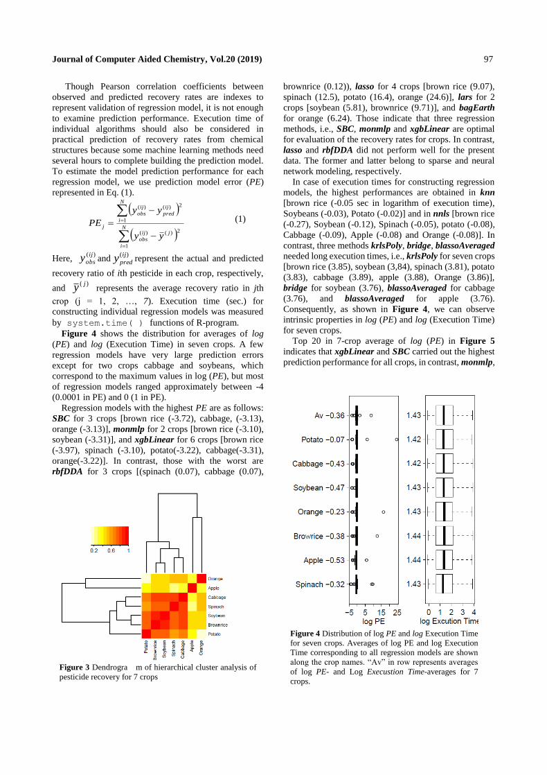
Figure 4 shows the distribution for averages of log

(PE) and log (Execution Time) in seven crops. A few

regression models have very large prediction errors

except for two crops cabbage and soybeans, which

correspond to the maximum values in log (PE), but most

of regression models ranged approximately between -4

(0.0001 in PE) and 0 (1 in PE).

Regression models with the highest PE are as follows:

SBC for 3 crops [brown rice (-3.72), cabbage, (-3.13),

orange (-3.13)], monmlp for 2 crops [brown rice (-3.10),

soybean (-3.31)], and xgbLinear for 6 crops [brown rice

(-3.97), spinach (-3.10), potato(-3.22), cabbage(-3.31),

orange(-3.22)]. In contrast, those with the worst are

rbfDDA for 3 crops [(spinach (0.07), cabbage (0.07),

brownrice (0.12)), lasso for 4 crops [brown rice (9.07),

spinach (12.5), potato (16.4), orange (24.6)], lars for 2

crops [soybean (5.81), brownrice (9.71)], and bagEarth

for orange (6.24). Those indicate that three regression

methods, i.e., SBC, monmlp and xgbLinear are optimal

for evaluation of the recovery rates for crops. In contrast,

lasso and rbfDDA did not perform well for the present

data. The former and latter belong to sparse and neural

network modeling, respectively.

In case of execution times for constructing regression

models, the highest performances are obtained in knn

[brown rice (-0.05 sec in logarithm of execution time),

Soybeans (-0.03), Potato (-0.02)] and in nnls [brown rice

(-0.27), Soybean (-0.12), Spinach (-0.05), potato (-0.08),

Cabbage (-0.09), Apple (-0.08) and Orange (-0.08)]. In

contrast, three methods krlsPoly, bridge, blassoAveraged

needed long execution times, i.e., krlsPoly for seven crops

[brown rice (3.85), soybean (3,84), spinach (3.81), potato

(3.83), cabbage (3.89), apple (3.88), Orange (3.86)],

bridge for soybean (3.76), blassoAveraged for cabbage

(3.76), and blassoAveraged for apple (3.76).

Consequently, as shown in Figure 4, we can observe

intrinsic properties in log (PE) and log (Execution Time)

for seven crops.

Top 20 in 7-crop average of log (PE) in Figure 5

indicates that xgbLinear and SBC carried out the highest

prediction performance for all crops, in contrast, monmlp,

Figure 3 Dendrogra m of hierarchical cluster analysis of

pesticide recovery for 7 crops

Figure 4 Distribution of log PE and log Execution Time

for seven crops. Averages of log PE and log Execution

Time corresponding to all regression models are shown

along the crop names. “Av” in row represents averages

of log PE- and Log Execustion Time-averages for 7

crops.


ppr, extraTrees, and xgbDART also show the highest

prediction performance for several crops. Execution times

of the top 20 ranged from 1.24 sec. to 46 min.

3.3 Generalized performance of regression methods

Generalized performance usually refers to the ability

of regression methods to be effective across a range of

input data and regression methods may always have

strengths and weaknesses. It is generally considered that

a single model is unlikely to fit every possible data and

ensemble regression methods trend to achieve higher

generalized performance than any of the ordinary models.

Ensemble regression makes it possible to obtain better

results when there is considerable diversity among the

base classifiers, regardless of the measure of diversity [21].

In the present analysis, the generalized performance in

different crops is the one of the topics for selecting

regression methods.

Average PEk for seven crops (j= 1, 2,…, M, and M

= 7) in kth regression method represented in Eq. (2) is one

of the indexes for generalized performance taking

different crops into consideration.

M

PE

PE

M

j

k

k

j

1

)(

(2)

In addition to PEk, average rank of kth method for

PEj(k), (k = 1, 2, …, 89) for seven crops becomes an index

of generalized performance for different crops. Thus we

compared between PEk and the average rank for

individual methods and obtained clear linear relationships

between them (Figure 6).

Top four regression methods, xgbLinear, SBC, ppr and

extraTrees are with the lowest PE with the best ranks. To

compare trends of regression methods, we classified 89

regression models to 11 categories in Table 1.

Figure 7 represents box plots for two performance rates,

i.e., log PE and average of log (Execution Time) for 11

categories of machine learning methods. It can be

observed that in terms of the median values of logPE, the

following three types of methods performed better: (i)

ensemble decision trees, (ii) ordinal kernel type of

regressions and (iii) ordinal centroid types of regressions

using distance function for individual samples. In addition

to those general trends, it should be worthy of notice that

methods belonging to ensemble simple linear and ordinal

centroid type also have very high performance in the

context of generalized prediction error represented by Eq.

(2).

On the execution time, ordinary neural network

regressions and ensemble-type of regressions using

decision trees and splines trend to need relatively long

execution time but this trend are opposite in ensemble-

type simple linear models. The performance rates in

prediction errors and execution times for 89 methods

(Appendix Table 1) are visualized in Figure 8. In the

present data, SBC and xgbLinear have the highest

performance in prediction errors, ppr and monmlp show

the second level performance; whereas gaussprLinear

and widely used lm are good methods in terms of

execution time.

Discussion

GC/MS is widely used for residual pesticide analysis in

foods, but the recovery rate is affected by several factors

such as sample preparation method and chemical

interactions of the flow path in GC/MS, such as the GC

inlet, column and ion source. Pesticides are very diverged

in chemical structures and are unstable chemical

compounds i.e., they undergo rapid degradation

(changing to non-toxic chemical species) in the

environment after use. Simultaneous analysis of multiple

pesticides is also challenging due to the matrix effects and

other factors in GC/MS. There are a lot of researches on

Figure 5 Averages of log PE for seven crops

corresponding to a number of regression methods


the recovery ratio of pesticides in foods for the sample

preparation methods [22-25]. Over- and underestimate of

recovery rate of pesticide cause the risk of food safety,

especially, false negative by the under estimate will

endanger the food safety of consumers. GC/MS is well

established technology over decades with the advantage

of stable ionization of EI and lower initial and operational

cost. Furthermore, the parameters for optimum method to

analyze the target pesticides have also developed for

reducing the matrix effect [22]. As reported by various

researches of pesticides in foods [26-28], the recovery rate

of pesticide is the important information, especially for

the QuEChERS (Quick, Easy, Cheap, Effective, Rugged

and Safe) method which is widely used globally for

chemical analysis of pesticides on foods for GC/MS.

There are several chemometrics studies on the pesticide

analysis using GC/MS [29,30] toward optimization of

GC/MS.

Experienced chemists can predict whether the new

compounds are GC amenable or not; and evaluate

recovery ratio of pesticides with the crops according to the

chemical structure based on unique functional groups (e.g.

carbamates, organophosphates, pyrethroids, etc..),

chemical bonding (resonance of pi-bonds, hydrogen

bonding effect, etc..), and matrix of the crops etc. This

human-dependent approach is also important but there are

risks of the m isjudgment that will cause the wrong

prediction resulting in the waste of energy and time for

analysis and sacrifice in food safety. In the present study,

Figure 6 Relationships between average of rank (X-axis) and PEk (Y-axis) for seven crops. The range of PEk is set between 0

and 1 because kth regression method with PEk larger than 1 means no prediction performance according to Eq. (1)


pesticides recovery rates for 7 crops are successfully

predicted based on molecular descriptors determined

using rcdk package and regression analysis methods of

caret package. Though correlation is weak between the

pesticide recovery and each molecular descriptor, we have

obtained several regression models with high prediction

performance and short execution times to predict recovery

rates based on molecular properties.

In the present work, we created 89 regression models

based on 10-fold cross validation and focused on

execution time as an important factor to adopt regression

models. We examined (i) prediction error, (ii) execution

time and (iii) generalized performance for selecting the

optimum machine learning methods for pesticide

recovery prediction. The execution time for constructing

the prediction model varies in method, and ensemble

learning methods required long execution time for the

nature of algorithms. In contrast, execution times for

linear regression models (lm) and general linear

regression models (glm) were less than 10 seconds. But

prediction rates for the lm and glm were not so good,

around PE = 0.1, i.e.10% of prediction error. The highest

accuracy (log(PE) <-3 across 7 crops) and reasonable

execution times (50 ~ 100 seconds) were observed in SBC

and xgbLinear. Thus, those two machine learning

methods are optimum for the present study.

The correlations between molecular descriptors and

recovery of pesticides are not so strong, ranged from -

0.254 to 0.523. The brown rice and soybean correspond to

relatively stronger correlations than the other crops. This

could be caused by the difference of the sample

preparation procedure of JPL method, i.e. removal of

lipids and difference in the residual matrix after sample

preparation. The hierarchical clustering makes it possible

to group crops according to the recovery rates of

pesticides, i.e. (i) cabbage and spinach, and (ii) soybean

and brown rice are highly related in the context of the

recovery rates of pesticides. Soybean and brown rice were

treated as the “grains, beans, nuts and seeds” and

underwent different clean-up methods from the other

crops. The profile of correlation of orange was different

from the other crops because of the difference of residuals

from orange after the sample treatment.

5 Conclusive Remarks

Pesticide recovery rates for vegetables and fruits using

GC/MS is influenced by different factors including the

matrix effect and chemical interactions between

pesticides and other mixing chemicals in crops. In the

present study, we recommend two machine learning

regression methods called SBC and xgbLiner in view of

prediction rates and execution times. In those two

regression models predictions of recovery rates of

pesticides are carried out in local distribution of chemical

properties among the 174 molecular descriptors. This

means that closely related pesticides in the chemical space

have also very similar recovery rates but explanation of

Figure 7 Box plots for log PE and average of log (Execution Time) for seven crops corresponding to 11 categories of regression

methods.


recovery rates based on similarities of molecular

properties are complicated because prediction errors of

recovery rates based on multilinear regressions such as lm,

glm, gaussprLinear is much larger than SBC and

xgbLiner. The formers make it possible to understand the

recovery rates by molecular descriptors on the basis of

linear relationships.

References and Notes

[1] Y. C., Lo, S. E. Rensi, W. Torng, B/ Altman, Drug

Recovery Today, 23 (2018) 1538-1546.

[2] D. Tilman, K.G.Cassman, P. A. Matson, R. Naylor,S.

Polasky Nature, 418 (2002) 671-677,

[3] B. K. Matuszewski, M. L. Constanzer, C. M. Chavez-

Eng, Anal. Chem., 75 (2003) 3019-3030.

[4] Katsuhiko KAWAMOTO and Nobuko MAKIHATA.,

2003).

[5] Alimentarius Commission, Codex general standard for

contaminants and toxins in food and feed (CODEX

STAN 193-1995),

http://www.fao.org/fileadmin/user_upload/livestockg

ov/documents/1_CXS_193e.pdf

[6] European Commission Health and Food Safety,

Regulation. [(accessed on 10 October 2016)];

Available online:

Figure 8 Relationships between average of log (PE) and average of log (Execution Time) for regression methods. Ordinary

learning and Ensemble learning methods corresponds to blue and red circles, respectively. Detail data is listed in Appendix

Table 1.


http://ec.europa.eu/food/plant/pesticides/max_residu

e_levels/eu_rules/index_en. htm.

[7] United States Department of Agriculture Maximum

Residue Limit Database. Foreign Agricultural Service

Department. Available online:

http:www.fas.usda.gov/maximum-residue-limits-

mrl-database.

[8] 厚労省、平成27年度食品中の残留農薬等検査

結果について (2015) https://www.mhlw.go.jp/stf/

seisakunitsuite/bunya/0000194458.html

[9] G. Fuleky, G., Cultivated plants, pprimarily as food

sources, UNESCO-EOLSS (2009) https://www.

eolss.net/Food-Agricultural-Sciences.aspx

[10] R. Guha, J. Statistical software, 18 (2007) 1-18.

[11] M. Kuhn, J. Statistical Software, 28 (2008) 1-26.

[12] N. Sadao, T. Yamagami, Y. Ono, K. Toubou, S.

Daishima, BUNSEKI KAGAKU 62, (2013) 229-241.

[13] Ministry of Health, Labour and Welfare in Japan,

Introduction of the Positive List System for

Agricultural Chemical Residues in Foods (2006).

[14] R. Tibshirani, J. Royal Statistical Soc. Ser. B, 59

(1997), 1948-1997.

[15] D. W. Marquardt, R. Snee, Am. Stat.,29 (1975) 3-20.

[16] N. S. Altman, Am. Stat. 46 (1992), 175-185.

[17] R.R. Yager, D. P. Filev, J. Intelligent Fuzzy Sys., 2

(1994), 209-219.

[18] A. G. Asuero , A. Sayago & A. G. Gonzalez, J.

Critical Rev. Anal. Chem., 46 (2006), 41-59.

[19] R. Bro, K. Kjeldahl, A. K. Smilde, H. A. L. Kiers,

Anal. Bioanal. Chem., 390 (2008), 1241-1251.

[20] K. Drab, M. Daszykowski, J. AOAC Int., 97, (2014),

29-38.

[21] L. I. Kuncheva, C. J. Whitaker, Machine Learning,

51 (2003), 181-207.

[22] P. Sandra, B. Tienpont, F. David, J. Chromatography

A, 1000 (2003), 299-309.

[23] K. Sugitate, M. Saka, T. Serino, S. Nakamura, A.

Toriba, K. Hayakawa, J. Agric. Food Chem., 60

(2012) 10226-10234.

[24] B. Lozowicka, E. Rutkowska, M. Jankowska,

Environ. Sci. Pollut. Res., 24 (2017) 7124- 7138.

[25] Raina, R.(2011) Chemical Analysis of Pesticides

Using GC/MS, GC/MS/MS, and LC/MS/MS,

Pesticides - Strategies for Pesticides Analysis, Prof.

Margarita Stoytcheva (Ed.)(2011).

[26] A. M. Filho, F. N. dos Santosa, P. A. de P. Pereira,

Talanta 81 (2010) 346-354.

[27] J. A. C. Guedes, R. O. Silva, C. G. Lima, M. A. L.

Milhome, R. F. do Nascimento, Food Chemistry, 199

(2016) 380-386.

[28] M. Tankiewicz Molecules 24 (2019) 417.

[29] L. B, Abdulra’uf, G. Huat Tan, Sample Prep., 2

(2015) 82-90.

[30] Yang Farina, Md Pauzi Abdullah, Nusrat Bibi, Wan

Mohd Afiq Wan Mohd Khalik Food Chemistry 224

(2017).


Appendix Table 1 Average of log PE (Av log PE) and Average of log Execution Time (Av log ET). Regression

methods (Method) are ordered according to Av log PE.

Method Av

logPE

Av log

ET Method

Av

logPE

Av log

ET Method

Av

logPE

Av

log

ET

xgbLinear -3.221 1.233 M5 -0.459 1.476 earth -0.199 0.782

SBC -3.124 1.416 kknn -0.457 0.473 BstLm -0.195 0.560

monmlp -2.002 1.743 svmLinear3 -0.434 1.040 knn -0.192 -

0.034

ppr -1.817 0.780 M5Rules -0.430 1.484 rpart2 -0.181 0.229

extraTrees -1.260 1.889 ridge -0.419 1.208 ctree2 -0.144 0.913

xgbDART -1.103 1.995 gaussprRadial -0.417 0.232 evtree -0.141 1.533

parRF -1.064 1.781 treebag -0.417 0.892 kernelpls -0.140 0.038

glm -0.963 0.015 svmLinear2 -0.403 0.813 plsRglm -0.133 1.702

lm -0.937 -0.050 penalized -0.386 1.405 widekernelpls -0.132 0.401

glmStepAIC -0.926 2.537 gcvEarth -0.371 0.549 lars2 -0.130 0.819

lmStepAIC -0.918 1.730 rpart1SE -0.347 0.204 ctree -0.127 0.573

qrf -0.894 1.745 neuralnet -0.343 1.784 simpls -0.124 0.015

bayesglm -0.809 0.887 svmRadialSigma -0.333 0.616 pls -0.122 0.024

brnn -0.783 2.272 cforest -0.328 1.528 blasso -0.119 3.208

ranger -0.757 1.552 enet -0.326 1.171 xyf -0.119 1.303

xgbTree -0.728 1.576 msaenet -0.315 1.777 superpc -0.078 0.447

RRFglobal -0.718 2.136 svmRadial -0.314 0.457 pcr -0.077 0.182

rf -0.717 1.778 svmRadialCost -0.314 0.312 leapForward -0.074 0.037

RRF -0.706 2.856 Rborist -0.310 1.691 leapBackward -0.072 0.155

krlsRadial -0.672 2.041 relaxo -0.304 1.009 leapSeq -0.070 0.121

rvmRadial -0.658 0.494 mlpML -0.281 1.147 icr -0.053 0.591

WM -0.649 2.877 glmnet -0.255 1.134 bridge -0.025 3.166

gaussprLinear -0.611 0.092 rvmLinear -0.253 0.443 dnn -0.011 1.822

svmPoly -0.576 0.971 spikeslab -0.252 1.225 blassoAveraged -0.007 3.183

bstTree -0.567 1.982 nodeHarvest -0.249 2.326 krlsPoly -0.005 3.312

rvmPoly -0.558 1.304 nnls -0.223 -0.098 rbfDDA 0.065 1.210

gbm -0.546 0.828 foba -0.215 1.129 bagEarth 0.542 1.785

gaussprPoly -0.534 0.698 mlpWeightDecay -0.204 1.562 lars 1.572 0.712

bagEarthGCV -0.475 1.397 glmboost -0.203 0.357 lasso 8.646 1.021

svmLinear -0.461 0.607 mlp -0.201 1.148

Chemoinformatics Approach for Estimating Recovery Rates of ...

Documents

Transcript of Chemoinformatics Approach for Estimating Recovery Rates of ...