Chasing the Tesla Standard: Predicting Battery Electric...
20
Jordan Cheng Mass-Market BEV Penetration Spring 2016 1 Chasing the Tesla Standard: Predicting Battery Electric Vehicle Sales amidst Increasing Competitive Pressures Jordan Cheng ABSTRACT Tesla has been a market leader in Battery Electric Vehicle (BEV) capabilities—boasting an EPA estimated travel range of 265 miles. Still, mass-market BEV manufacturers have been able to sell cars with a lower range of approximately 87 miles without having to make significant upgrades to their capacity. This is because Tesla vehicles—though powerful—are above the price point of the typical consumer. But in the next few years—anticipating Tesla’s release of an equally powerful mass-market vehicle—companies are preparing to release their next generation of BEVs. Recently, Chevy announced their next generation of BEVs will have a 200 mile travel capacity—which can be seen as an effort to compete with Tesla’s mass market vehicle. Based on this evidence, this paper examines the effect of travel range on sales of battery electric vehicles. Using sales data from hybridcars.com, I conducted an econometric analysis of factors that affect BEV adoption using a multivariate regression model with both fixed variable effects and fixed time effects. The main dependent variable of interest was monthly vehicle sales while the main independent variable of interest was travel range. Other independent variables such as gasoline prices and vehicle prices were included to help isolate the effect that travel range has on BEV sales. Through various iterations of the multivariate regression model, the linear coefficient of travel range regressed on sales remained positive and statistically significant (p<0.01) with a with an approximate 5.4-5.6% increase for every additional mile of range. KEYWORDS Tesla Model III, Travel Range, Econometric Analysis, Travel Range Anxiety, Vehicle Adoption
Transcript of Chasing the Tesla Standard: Predicting Battery Electric...

Jordan Cheng Mass-Market BEV Penetration Spring 2016
1
Chasing the Tesla Standard: Predicting Battery Electric Vehicle Sales amidst Increasing
Competitive Pressures
Jordan Cheng
ABSTRACT
Tesla has been a market leader in Battery Electric Vehicle (BEV) capabilities—boasting an EPA estimated travel range of 265 miles. Still, mass-market BEV manufacturers have been able to sell cars with a lower range of approximately 87 miles without having to make significant upgrades to their capacity. This is because Tesla vehicles—though powerful—are above the price point of the typical consumer. But in the next few years—anticipating Tesla’s release of an equally powerful mass-market vehicle—companies are preparing to release their next generation of BEVs. Recently, Chevy announced their next generation of BEVs will have a 200 mile travel capacity—which can be seen as an effort to compete with Tesla’s mass market vehicle. Based on this evidence, this paper examines the effect of travel range on sales of battery electric vehicles. Using sales data from hybridcars.com, I conducted an econometric analysis of factors that affect BEV adoption using a multivariate regression model with both fixed variable effects and fixed time effects. The main dependent variable of interest was monthly vehicle sales while the main independent variable of interest was travel range. Other independent variables such as gasoline prices and vehicle prices were included to help isolate the effect that travel range has on BEV sales. Through various iterations of the multivariate regression model, the linear coefficient of travel range regressed on sales remained positive and statistically significant (p<0.01) with a with an approximate 5.4-5.6% increase for every additional mile of range.
KEYWORDS
Tesla Model III, Travel Range, Econometric Analysis, Travel Range Anxiety, Vehicle Adoption

Jordan Cheng Mass-Market BEV Penetration Spring 2016
2
INTRODUCTION
Electric vehicles are often seen as a cleaner alternative to fuel-based vehicles as they tend
to have lower carbon emissions. While there are a variety of electric vehicles, Battery Electric
Vehicles (BEV) have the greatest potential for carbon independence as they are completely
battery powered. However, there are a number of drawbacks that leave BEVs infeasible for mass
market penetration such as limited travel range, long charging times, and a lack of charging
infrastructure. Tesla, a BEV manufacturer, has made efforts to curb these disadvantages through
technological innovations and implementation of their own charging stations. But, where they
really pose a competitive advantage in the BEV industry is in their travel range. Compared to the
industry average range of 87 to 124 miles, Tesla boasts a much larger range of 265 miles
(Hardman 2015, Electrification Coalition 2012). Until recently, Tesla vehicles have largely been
inaccessible to the mass-market due to their high prices. This changed with the announcement of
the intended release of the Model III, a $35,000 vehicle with a 215 mile range (teslamotors.com
2016). A more affordable class of their vehicles could have large implications for the EV market,
on the whole. Tesla’s competitive advantage in travel range paired with their new mass-market
appeal will force other automakers to make comparable improvements to compete or risk losing
market share.
Prior to Tesla’s announcement, Chevrolet announced their plans to release their next
generation BEV—the Bolt—which is expected to have a 200 mile range starting at $37,500
(hybridcars.com 2016). This is significant as Chevrolet’s previous BEV—the Spark—had an 84
mile capacity. To drastically increase their travel range from 84 to 200 miles is somewhat
arbitrary without context. However, Tesla’s mass-market Model III has been a publicly known
part of their business plan for many years now (Musk 2006). As a result, despite the Bolt’s
earlier announcement and release date, Chevrolet’s rapid technological improvements can be
seen a direct response to the upcoming Tesla Model III. As Chevrolet leads the charge in
competing with Tesla on travel range, this leaves speculation on the market as a whole. Will
other automakers make similar improvements to their BEVs?
If other automakers were to also increase the travel range of their BEVs, this could have a
significant impact on the BEV industry due to changes in consumer sentiment. According to the
Electrification Coalition, 68% of Americans travel less than 40 miles per day (Electrification

Jordan Cheng Mass-Market BEV Penetration Spring 2016
3
Coalition, 2013). At this level of driving demand, BEVs in their current state should suffice for
the majority of the public. Still, consumers cite travel range as one of the main reasons for not
purchasing a BEV (Electrification Coalition 2013). This may be due to the fear of being stranded
with little to no charge—which is typically referred to as range anxiety (Nillson 2011). Range
anxiety can be partially alleviated through measures like increased availability of charging
infrastructure, free roadside assistance, and remote access to the status of the car (Nillson 2011).
However, because data shows that the onset of range anxiety tends to occur when the charge falls
below 50%, it can be addressed by simply increasing the travel range (Caroll 2010). With rapid
improvements in travel range imminent, consumers may become more inclined to switch over to
BEVs.
While consumer preferences for travel range have been well studied, information about
its market influence is limited. Previous studies have touched on the subject of travel range
without it being the main focus. For example, one study was conducted via survey to find
factors that are most influential in a consumer’s purchasing decision (Egbue and Long 2012). As
travel range was identified as the biggest concern, its market impact is not quantified. In an
econometric study, factors such as incentives, fuel prices, income, and vehicle price were used to
study their market impact—but lacked analysis on travel range (Sierzchula et al. 2014).
Contrastingly, this study attempts to discover how improvements in travel range can affect BEV
sales in the US market.
Using a simple multi-variable fixed effects regression, this study estimates the linear
relationship between travel range and sales of BEVs. In order to accomplish this, other
exogenous variables affecting the sales of BEVs must be incorporated into this model to isolate
the true effect of travel range on sales. Within the scope of this study, gasoline prices and
vehicle prices are identified as the other main contributors to the sale of a BEV. Under general
economic intuition, vehicle pricing is identified as a factor because as prices increase, we should
expect to see quantity sold to decline. This relationship is enforced with Egbue and Long’s study
on consumer attitudes where they find that cost is the second most important factor when
considering BEV adoption (Egbue and Long 2012). Gasoline prices are included into the study
as they are also influential in the decision making process. As gas prices increase, the operational
costs of conventional vehicles also increase. When conventional vehicles are costlier to operate,
consumers have more incentive to switch to alternatively-fueled vehicles like a BEV. This

Jordan Cheng Mass-Market BEV Penetration Spring 2016
4
relationship can be observed in the hybrid electric vehicle market where gas prices were
positively correlated with sales (Gallagher and Muehlegger 2011). Additionally, fixed entity
effects are included to account for inherent differences in automakers. For example, some
models like the Nissan Leaf have more sales due to its earlier release while the Smart Car may
have lower sales due to its lower perceived vehicle safety. Lastly, time-fixed effects account for
conditions that may vary across time such as macro-economic conditions. When the U.S.
economy is not doing as well, vehicle sales may decline as well. The strength and directions of
these variables’ relationship to sales will allow me to estimate the effects industry improvements.
BACKGROUND
Electric Vehicles (EVs) come in many forms—each varying in the amount that they rely
on an electric battery. A Hybrid Electric Vehicle (HEV) captures the energy normally lost to
braking but still heavily relies on its internal combustion engine (Pappas 2014). While HEVs
rely greatly on their combustion engine, a Plug-In Hybrid Vehicle (PHEV) is less gasoline
dependent. A PHEV can plug into an outlet to charge a battery, and typically runs about 40
miles before switching to its gasoline-powered internal combustion engine (Pappas 2014).
Finally, purely electric vehicles—known as Battery Electric Vehicles (BEV)—have the longest
battery powered travel capacity of the suite of EVs, but still do not have the same travel range of
combustion engines. Due to their compatibility with current gasoline infrastructure, HEVs have
been the most commercially successful electric vehicle since the invention of the Toyota Prius in
1997 (Matulka 2014).
While HEVs are the most popular of the electric vehicles, they are still vastly out-
numbered by traditional internal combustion vehicles (ICVs). As of October 2015, hybrid
electric vehicle sales constituted a 2.25% share of all light duty vehicles --or about 320,000 units
(Zhou 2015). Hybrid Electric Vehicle sales have been on the rise since 1999. Their market share
of all new, light-duty vehicle sales rose to a peak of about 3.2% in 2013 (Zhou 2015). However,
a paper on the consumer response to gasoline pricing reports that the elasticity of driving demand
when compared to the price of gasoline is approximately -.15 (Gillingham 2011). As a result, the
decline in gasoline prices since 2013 may explain the decline in HEV sales in recent years
(Energy Information Administration 2015). PHEVs constitute smaller fraction of total vehicle
Jordan Cheng Mass-Market BEV Penetration Spring 2016
5
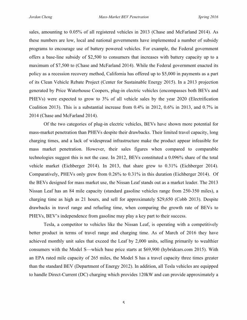
sales, amounting to 0.05% of all registered vehicles in 2013 (Chase and McFarland 2014). As
these numbers are low, local and national governments have implemented a number of subsidy
programs to encourage use of battery powered vehicles. For example, the Federal government
offers a base-line subsidy of $2,500 to consumers that increases with battery capacity up to a
maximum of $7,500 to (Chase and McFarland 2014). While the Federal government enacted its
policy as a recession recovery method, California has offered up to $5,000 in payments as a part
of its Clean Vehicle Rebate Project (Center for Sustainable Energy 2015). In a 2013 projection
generated by Price Waterhouse Coopers, plug-in electric vehicles (encompasses both BEVs and
PHEVs) were expected to grow to 3% of all vehicle sales by the year 2020 (Electrification
Coalition 2013). This is a substantial increase from 0.4% in 2012, 0.6% in 2013, and 0.7% in
2014 (Chase and McFarland 2014).
Of the two categories of plug-in electric vehicles, BEVs have shown more potential for
mass-market penetration than PHEVs despite their drawbacks. Their limited travel capacity, long
charging times, and a lack of widespread infrastructure make the product appear infeasible for
mass market penetration. However, their sales figures when compared to comparable
technologies suggest this is not the case. In 2012, BEVs constituted a 0.096% share of the total
vehicle market (Eichberger 2014). In 2013, that share grew to 0.31% (Eichberger 2014).
Comparatively, PHEVs only grew from 0.26% to 0.31% in this duration (Eichberger 2014). Of
the BEVs designed for mass market use, the Nissan Leaf stands out as a market leader. The 2013
Nissan Leaf has an 84 mile capacity (standard gasoline vehicles range from 250-350 miles), a
charging time as high as 21 hours, and sell for approximately $29,650 (Cobb 2013). Despite
drawbacks in travel range and refueling time, when comparing the growth rate of BEVs to
PHEVs, BEV’s independence from gasoline may play a key part to their success.
Tesla, a competitor to vehicles like the Nissan Leaf, is operating with a competitively
better product in terms of travel range and charging time. As of March of 2016 they have
achieved monthly unit sales that exceed the Leaf by 2,000 units, selling primarily to wealthier
consumers with the Model S—which base price starts at $69,900 (hybridcars.com 2015). With
an EPA rated mile capacity of 265 miles, the Model S has a travel capacity three times greater
than the standard BEV (Department of Energy 2012). In addition, all Tesla vehicles are equipped
to handle Direct-Current (DC) charging which provides 120kW and can provide approximately a
Jordan Cheng Mass-Market BEV Penetration Spring 2016
6
50% charge to vehicles in 30 minutes whereas other vehicles may require additional payments
(Hardman 2015).
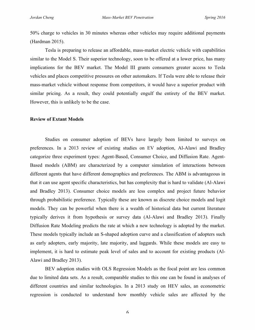
Tesla is preparing to release an affordable, mass-market electric vehicle with capabilities
similar to the Model S. Their superior technology, soon to be offered at a lower price, has many
implications for the BEV market. The Model III grants consumers greater access to Tesla
vehicles and places competitive pressures on other automakers. If Tesla were able to release their
mass-market vehicle without response from competitors, it would have a superior product with
similar pricing. As a result, they could potentially engulf the entirety of the BEV market.
However, this is unlikely to be the case.
Review of Extant Models
Studies on consumer adoption of BEVs have largely been limited to surveys on
preferences. In a 2013 review of existing studies on EV adoption, Al-Alawi and Bradley
categorize three experiment types: Agent-Based, Consumer Choice, and Diffusion Rate. Agent-
Based models (ABM) are characterized by a computer simulation of interactions between
different agents that have different demographics and preferences. The ABM is advantageous in
that it can use agent specific characteristics, but has complexity that is hard to validate (Al-Alawi
and Bradley 2013). Consumer choice models are less complex and project future behavior
through probabilistic preference. Typically these are known as discrete choice models and logit
models. They can be powerful when there is a wealth of historical data but current literature
typically derives it from hypothesis or survey data (Al-Alawi and Bradley 2013). Finally
Diffusion Rate Modeling predicts the rate at which a new technology is adopted by the market.
These models typically include an S-shaped adoption curve and a classification of adopters such
as early adopters, early majority, late majority, and laggards. While these models are easy to
implement, it is hard to estimate peak level of sales and to account for existing products (Al-
Alawi and Bradley 2013).
BEV adoption studies with OLS Regression Models as the focal point are less common
due to limited data sets. As a result, comparable studies to this one can be found in analyses of
different countries and similar technologies. In a 2013 study on HEV sales, an econometric
regression is conducted to understand how monthly vehicle sales are affected by the

Jordan Cheng Mass-Market BEV Penetration Spring 2016
7
implementation of different government incentives (Jenn et al. 2013). Using monthly vehicle
sales the dependent variable, Jenn (2013) analyzes correlations with explanatory variables such
as government incentives like cash for clunkers, advertising campaigns, and macroeconomic
factors like gasoline prices. The regression equation below represents their OLS estimation
where Si,t represents monthly vehicle sales by model, EPACTi,t is the dollar incentive for the
vehicle model in the time period, xi,t is a control variable, and ui is unobserved car
characteristics.
ln(Si,t)=α+πln(Si,t−1)+β(EPACTi,t)+γ(xi,t)+ui+εi,t
Another OLS study was conducted with data from 30 different countries but only used data in
the year 2012 (Sierzchula et al. 2014). Rather than using panel data, this study analyzes financial
incentives and socioeconomic factors that vary with location. On the left side of the OLS
regression equation below is the dependent variable is the log of the market share that BEVs hold
in country (i). On the right side are the dependent variables consisting of incentives and
socioeconomic factors in country (i).
log_MarShri=α+β1Incentivei+β2Urbandensityi+β3Educationi+β4Envi+β5Fueli
+β6ChgInfi+β7Elec+β8PerCapVehicles+β9EV_Price+β10Availability+β11Introduction+β12HQ+εi
Study Model
The model used to analyze the effect of travel range on BEV sales reflects similar
methods listed above. To estimate the effect of travel range on BEV sales, I used an Ordinary
Least Square (OLS) regression of sales on multiple explanatory variables. The study is similar to
both Jenn’s (2013) model in that it uses panel data and the log of sales as the independent
variable while sharing some explanatory variables with Sierzchula’s (2014) model. By using the
log of sales, this gives an approximation for the percentage increase in sales as opposed to
nominal increases. However, this study differs by using time-fixed effects to account for
unobservable time variant factors. Listed below is the OLS model used to isolate the effect of
travel range on sales and a description of all the variables.

Jordan Cheng Mass-Market BEV Penetration Spring 2016
8
ln(SYZ) = β[ + β\XYZ + β^YZ + β`ZYZ + αYZ + FY + TZ + εYZ
Variable Description
SYZ SalesofCarModel i intimeperiod t inunits
β[ Intercept(BaselinelevelofBEVadoption)
β\ EffectofTravelRangeonSales
XYZ TravelRangeofCarModel i intimeperiod t inmiles
β^ EffectofGasolinePricesonSales
YZ AverageUSGasolinePriceintimeperiod t in$
β` EffectofVehiclePriceonSales
ZYZ PriceofCarModel i intimeperiod t in$
αYZ Bivariatedummyvariabletoidentifywhencarisfirstthreemonthsonsale
FY FixedEntityEffectofCarModelonSales
TZ MonthlyTimeFixedEffectonSales
εYZ ErrorTerm
From this regression output, I will use the linear relationship between travel range and log of
sales to estimate the percentage increase in sales.
METHODOLOGY
Data Collection
I collected data on four different variables—BEV sales, travel range, vehicle price, and
gasoline prices—up until March of 2016. Because discovering travel range’s relationship to sales
is the primary goal of this study, the panel data revolved around available sales information.
BEV sales data only dates back a few years and as a result, annual data is not conducive for
statistical tests. However, monthly figures were publicly available and effectively increased the
sample size. In Jenn’s (2013) regression analysis on HEV sales, monthly sales were used as
Table 1. Variable Descriptions. A list of descriptions for all the variables used in OLS Model

Jordan Cheng Mass-Market BEV Penetration Spring 2016
9
opposed to annual sales. Monthly figures also provide other advantages such as being able to
account for more fluctuation in travel range, gas prices, and vehicle prices. Using this intuition,
monthly figures were used instead of annual figures.
BEV Sales
Similar to Jenn’s study on HEV adoption, I sourced monthly BEV sales data listed on
hybridcars.com (Jenn et al. 2013). Hybridcars.com is a source that has been cited by the U.S.
Department of Energy and is a reputable source for these figures.
BEV Travel Range
To collect data on travel range, I used the Department of Energy’s fueleconomy.gov to
retrieve the BEV’s EPA estimated ranges. While travel ranges may vary between websites, using
the EPA estimated range keeps the standard relatively consistent. The listed travel ranges are
based on automaker’s submitted test results which can result in some bias (EPA 2015). However,
the EPA may conduct its own tests and change the listed range if there are discrepancies (EPA
2015). This keeps the standard across automakers relatively consistent and reflects what the
consumer would encounter in a market situation.
Vehicle Price
To further isolate the effect of travel range on sales, I sourced vehicle prices from the
Department of Energy’s fueleconomy.gov. If multiple vehicle prices were available for the
model, a simple arithmetic average was calculated. Because vehicle prices change between
years, I populated my dataset according to their release date. If a release date was accessible, I
would change the vehicle price starting that month. However, if a release date was not listed, I
listed the new price exactly 12 months after the previous model year was released.
Gasoline Price

Jordan Cheng Mass-Market BEV Penetration Spring 2016
10
As gasoline prices play a role in consumer’s perceptions of electric vehicles, I sourced
information on prices from the energy information administration (EIA). Gasoline prices were
denominated in dollars per gallon. For each month/year that was listed, I referenced EIA and
listed the average monthly gasoline prices. Average gasoline price was held consistent across
vehicle models for each month.
Data Manipulation
During the data collection process, I noticed some data irregularities and accounted for
these using bi-variate dummy variables and deletion. A dummy variable I generated was for the
first three months of sale. If a car was in its first three months of sales, it would generate a “1”
while the rest would be zero. In the first few months of sales there are shipment delays that
significantly reduce the figures. At the end of 2015, both the Toyota Rav4 EV and Honda Fit EV
concluded their production and their sales declined drastically. As a result, I deleted the sales
data for both the Rav4 and the Fit EV after production ended.
The data was organized into panel form which contains both the vehicle model and the
date. In doing so, I am able to account for differences in vehicle attributes (fixed entity effects)
and time-specific conditions like macroeconomic fluctuations (time fixed effects)—both of
which are non-measurable parameters. As a result, I encoded the car model variable and the date
variable for Stata to interact properly. Using the encode function, I generated the variable model1
and date1 to use for regression.
Additionally, from a surface level interpretation of sales data, Tesla BEV sales appear
abnormally high despite higher costs. This may be due to the fact that Tesla vehicles may be
viewed as luxury vehicles as opposed to BEVs. If this is the case, consumers of the Model S are
not interested in the BEV for pure functionality. As a result, a second pool of data without
Tesla’s sales is generated and used for analysis.
Dataset Summary
My final pool of data came down to seven variables (sales, ln sales, travel range, gas
price, vehicle price, dummy variable for the first three months, vehicle model, and date) and had

Jordan Cheng Mass-Market BEV Penetration Spring 2016
11
438 observations. The model and date variables were not encoded for Stata to interact properly
initially. Model1 and date1 were generated and encoded for Stata to run fixed time effects and
time fixed effects regression. Four continuous variables (Sales, Range, Gas Price, and Price)
were also included (Table 2).
Variable Observations Mean Std. Dev. Min Max
Model 0
Date 0
Sales 438 458.3174 719.7436 0 3202
Range 438 96.80594 51.09295 62 257
Gprice 438 3.108667 .6021555 1.872 3.96
Price 438 37590.36 16651.5 22995 88800
Fthree 438 .0753425 .264245 0 1
Model1 438 6.508132 3.281679 1 12
Date1 438 33.09361 18.69037 1 64
lnsales 431 4.965569 1.676143 0 8.071531
Additionally, I plotted the two main variables of interest—Sales and Travel Range—and
discovered a general positive relationship (Figure 1). Within this scatterplot, there are two major
clusters observable. On the left end of the graph are standard BEVs, and on the right are Tesla
BEVs.
0500
100015002000250030003500
50 100 150 200 250Mon
thlyVeh
icleSales
TravelRange
Sales
Linear(Sales)
Table 2. Summary Statistics. Summary statistics for complete data set. Table includes the manipulations included in Stata.
Figure 1. Sales and Range Scatterplot. Scatterplot with line of best-fit of two main variables of interest: sales and travel range.

Jordan Cheng Mass-Market BEV Penetration Spring 2016
12
Econometric Analysis
In order to isolate the effect of travel range (𝛽\) on sales (𝑆lm) I ran a multivariate
regression with sales as the dependent variable in Stata 13 (Statacorp 2013). I set the fixed
effects (time and entity) by using the xtset function. I conducted different combinations of
regressions using the xtreg function with sales as the dependent variable. For the full regression,
I regressed the log of sales on travel range, price, gasoline price, first three months of sale, and
included the fixed time effect and fixed entity effects. This generated regressions useful for
analyzing for the effect of BEV travel range on sales. Using these procedures, I generated
models useful for analyzing for the effect of BEV travel range on sales.
ln(SYZ) = β[ + β\XYZ + β^YZ + β`ZYZ + αYZ + FY + TZ + εYZ
RESULTS
Regression Results
In Model 1, I used all the collected variables to estimate the effect of travel range on BEV
sales. Running the regression without the fixed effects, all the coefficients were statistically
significant at a 99% confidence level (p < 0.01). Not accounting for fixed effects, for every
additional mile of travel range, this would result in a 3.9% increase in sales. In addition, for
every additional dollar in gasoline price we would expect a 39.8% increase and for every
thousand dollar increase. In terms of vehicle price, its effect appears to equal zero. However, as
noted in the non-log transformation iteration of the regression in column 1, it is lowly negative.
This is consistent with the intuition that as vehicle price increase, sales would decrease.
However, when time fixed effects are included, gas price and vehicle price lose their statistical
significance (Model 1). As a result, the model was adjusted – resulting in Model 2.
Jordan Cheng Mass-Market BEV Penetration Spring 2016
13
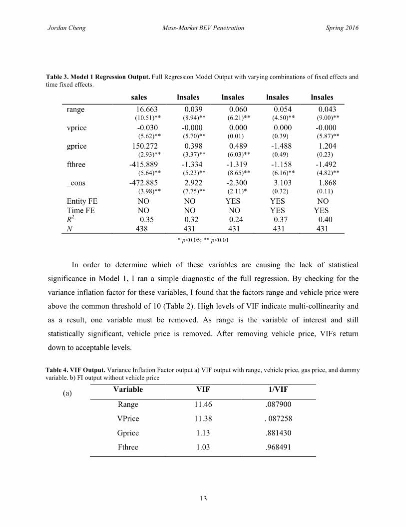
sales lnsales lnsales lnsales lnsales range 16.663 0.039 0.060 0.054 0.043 (10.51)** (8.94)** (6.21)** (4.50)** (9.00)** vprice -0.030 -0.000 0.000 0.000 -0.000 (5.62)** (5.70)** (0.01) (0.39) (5.87)** gprice 150.272 0.398 0.489 -1.488 1.204 (2.93)** (3.37)** (6.03)** (0.49) (0.23) fthree -415.889 -1.334 -1.319 -1.158 -1.492 (5.64)** (5.23)** (8.65)** (6.16)** (4.82)** _cons -472.885 2.922 -2.300 3.103 1.868 (3.98)** (7.75)** (2.11)* (0.32) (0.11) Entity FE NO NO YES YES NO Time FE NO NO NO YES YES R2 0.35 0.32 0.24 0.37 0.40 N 438 431 431 431 431
* p<0.05; ** p<0.01
In order to determine which of these variables are causing the lack of statistical
significance in Model 1, I ran a simple diagnostic of the full regression. By checking for the
variance inflation factor for these variables, I found that the factors range and vehicle price were
above the common threshold of 10 (Table 2). High levels of VIF indicate multi-collinearity and
as a result, one variable must be removed. As range is the variable of interest and still
statistically significant, vehicle price is removed. After removing vehicle price, VIFs return
down to acceptable levels.
Variable VIF 1/VIF
Range 11.46 .087900
VPrice 11.38 . 087258
Gprice 1.13 .881430
Fthree 1.03 .968491
Table 3. Model 1 Regression Output. Full Regression Model Output with varying combinations of fixed effects and time fixed effects.
Table 4. VIF Output. Variance Inflation Factor output a) VIF output with range, vehicle price, gas price, and dummy variable. b) FI output without vehicle price
(a)

Jordan Cheng Mass-Market BEV Penetration Spring 2016
14
Variable VIF 1/VIF
Range 1.00 .999784
Gprice 1.03 .971801
Fthree 1.03 .971940
In Model 2, I included travel range, gas prices, and the dummy variable that indicates the
first three months of distribution. Without fixed effects, only range and fthree remained
statistically significant at a 99% confidence level (p<0.01). With the inclusion of entity fixed
effects, gasoline prices became statistically significant as well. However, with the inclusion of
time fixed effects, gasoline prices lost its significance again. Due to the lack of statistical
significance in gasoline prices, time fixed effects appears incompatible with this gas prices. In
column 5 of Model 2, the regression is run with both fixed effects without the gas price variable.
In this iteration of the regression, every additional mile in range would result in a 5.6% increase
in BEV sales.
lnsales lnsales lnsales lnsales lnsales range 0.015 0.060 0.056 0.016 0.056 (11.38)** (6.30)** (5.15)** (11.45)** (5.18)** gprice 0.193 0.490 -1.460 1.268 (1.65) (6.28)** (0.49) (0.23) fthree -1.421 -1.319 -1.171 -1.472 -1.161 (5.39)** (8.67)** (6.33)** (4.55)** (6.32)** Entity FE NO YES YES NO YES Time FE NO NO YES YES YES _cons 2.991 -2.297 3.138 0.778 -1.482 (7.66)** (2.22)* (0.33) (0.04) (1.18) R2 0.27 0.24 0.37 0.35 0.37 N 431 431 431 431 431
* p<0.05; ** p<0.01
Using the results of the previous regression, I ran an analysis excluding Tesla BEVs
(Model 3). In the initial regression in column 1, range and the fthree dummy variable are
Table 5. Model 2 Regression Output. Regression Model Output with varying combinations of fixed effects and time fixed effects without vehicle price.
(b)

Jordan Cheng Mass-Market BEV Penetration Spring 2016
15
statistically significant at the 99% confidence level (p<0.01) while gas price is significant at the
95% confidence level (p<0.05). When accounting for entity fixed effects, the results of the
regression appear to indicate that for every additional mile of travel range should result in a 5.6%
to 6.7% increase in sales. For every dollar increase in gasoline prices, sales are expected to
increase by 55%.
lnsales lnsales lnsales lnsales range 0.025 0.067 0.056 0.031 (3.71)** (4.55)** (3.17)** (4.25)** gprice 0.269 0.546 (2.07)* (6.36)** fthree -1.328 -1.249 -1.137 -1.561 (4.57)** (7.59)** (5.63)** (4.39)** Entity FE NO YES YES NO Time FE NO NO YES YES _cons 1.950 -2.277 -0.746 3.736 (2.68)** (1.76) (0.50) (2.25)* R2 0.08 0.19 0.34 0.18 N 386 386 386 386
* p<0.05; ** p<0.01
DISCUSSION
The goal of this study was to confirm and isolate the effect of travel range improvements
on battery electric vehicle adoption. In this aim, I conducted multi-variable regression analyses
of different factors that may affect adoption of BEVs. Variables such as gasoline prices, vehicle
prices, and fixed-effects were used to isolate the effect of travel range. As fixed-effects were
included, some of these variables lost their statistical fit within the regression mode due to
potential collinearity. However, with each additional explanatory variable (gasoline prices,
vehicle prices, fixed effects) included into the regression model, the coefficient of travel range on
BEV adoption became less positive. This is indicative that the cumulative effect of variables
other than travel range has a negative effect on sales.
One of the hypotheses I made in this study was that gasoline prices would be positively
correlated to adoption of BEVs. I reasoned that if gas prices increased, consumers would likely
Table 6. Model 3 Regression Output. Regression Model Output with varying combinations of fixed effects and time fixed effects without vehicle price and excluding Tesla BEVs.

Jordan Cheng Mass-Market BEV Penetration Spring 2016
16
shy away from gasoline-dependent vehicles and embrace clean-energy alternatives, like BEVs.
This along with other studies has shown that this is typically the case (Sierzchula et al. 2014).
Without including fixed-effects, gasoline appeared to have a positive and statistically significant
correlation with monthly BEV sales. However, once time fixed effects were included in the
regression, gasoline prices lost their statistical significance (p>0.05). Including time fixed-
effects into my regression may have introduced collinearity. As time fixed-effects accounts for
variations in time, it shares a degree of correlation with monthly gasoline prices. Moreover, I
used nationwide average retail prices whereas BEV consumers may be concentrated in specific
regions, or they might encounter different effective gasoline prices from this average. As a result,
gasoline prices’ correlation with BEV adoption may have significance, but it appears to lack
compatibility with a time fixed-effects regression.
Another variable that I predicted to alter the adoption rate of BEVs was the base price of
the vehicle. Considering basic economic intuition, as the price of a vehicle increases, one should
expect sales to decline. My regression model did yield a negative coefficient for this relationship,
but this variable also lost significance and became positive when fixed variable-effects were
included into the regression. Variance inflation factor analysis indicated that vehicle price had a
high degree of collinearity with travel range. The collinearity between vehicle price and travel
range would again indicate that this vehicle price does not fit within the regression model. This
seems logical because as battery size increases, we would expect a higher inherent price of the
vehicle. However, the collinearity between these two variables indicates a difficulty in
conducting BEV adoption analysis. Both travel range and vehicle price are important factors that
consumers consider when purchasing a BEV, but it is hard to measure their effects
simultaneously. Despite this setback, consumer preference surveys can attempt to quantify their
individual effects.
Finally, I predicted increases in travel range to have a positive effect on sales.
Throughout the iterations of the multivariate regression, travel range consistently remained
statistically significant and had a positive correlation with BEV sales. Between the iterations, the
incremental effect of travel range on monthly BEV sales varied from a 1.5% to 6.5% increase in
sales per additional mile in range. However, when accounting for regression iterations that
include entity and time fixed-effects, the coefficient narrowed to a range of 5.4% to 5.6%. In
finding the correlation between vehicle adoption and travel range, I expected to see higher BEV

Jordan Cheng Mass-Market BEV Penetration Spring 2016
17
sales with higher battery capacity. As seen with Chevrolet’s move to make a rapid increase from
an 84 mile range vehicle to a 200 mile range, these competitive pressures may result in rapid
improvements across the board. However, it is interesting to note that even when vehicle pricing
was removed from the regression model, the coefficient of travel range versus BEV sales
remained positive. This seems to indicate that the preference for higher travel ranges has greater
influence on vehicle sales than negative effects of higher pricing. On a surface level
extrapolation, this may indicate that current BEV customers have other motivations behind their
purchases that extend beyond economic incentives.
Limitations
Deeper insights into the industry are hard to extrapolate given the extent of this study.
The methods for tallying of monthly auto sales were not explicitly stated from hybridcars.com
nor were they mentioned in similar sites like the Auto News Data Center. As a result, further
manipulations of the data set were not possible due to this limitation. For example, if sales were
sourced directly from the DMV with sale prices, further analysis of demand with relation to
pricing could be estimated. In addition, the actual purchase price of the vehicle may vary
depending on the add-on features, taxations, or subsidies that are applied. Therefore, assumptions
made in this study—like using the lowest-listed MSRP price—were used to accommodate this
limitation, but may skew the coefficients retrieved from the regression analysis. Moreover,
measures such as availability of charging infrastructure were not included in the study as it is
difficult to achieve accurate data due to the lack of information from private entities such as
private parking structures. Lastly, this study suffers from the lack of a long time-series. Mass-
market BEVs only date back a few years and major automakers are still absent from the market.
Future Directions
Further econometric studies may gain more explanatory power in predicting BEV
adoption as these vehicles mature in a technological sense and gain more mass-market traction.
As indicated from the results in this study, the incompatibility between travel range and vehicle
prices makes it difficult to conduct a more refined econometric analysis. Consumer preference

Jordan Cheng Mass-Market BEV Penetration Spring 2016
18
surveys that further examine these two variables may allow for more insight on their individual
effects. Even within this year, pre-orders for the $35,000 Tesla Model 3 have begun (ABC News
2016). Alongside the Chevrolet Bolt, sales from the new generation of mass-market and long-
distance BEVs will provide data for greater insight into the market and consumer demand for
these vehicles. Additionally, this type of econometric analysis can be applied to other markets
abroad or even sized down to smaller geographic regions such as the state of California. Smaller
geographic regions allow for closer analysis of factors that affect BEV sales, such as being able
to quantify the availability of charging infrastructure, which is difficult to accomplish in a
nationwide analysis.
While the nature of this research project appears to be an attempt to look at the near
future, the implications of a vastly changing vehicle network are massive. BEVs depend on
different modes of energy production than conventional vehicles. As a result, knowing the rate of
adoption of BEVs will allow for utilities to accurately predict the additional grid capacity needed
to power these vehicles. In addition, the widespread adoption of BEVs has the potential to reduce
the nation’s carbon footprint by reducing America’s reliance on gasoline. However, the actual
benefit of BEVs depends on the energy portfolio of grid systems currently in place. Knowing the
rate of BEV implementation will help determine the immediate impact of a cleaner energy
portfolio on society. In general, having a more accurate forecast of BEV adoption will allow for
policy leaders to make well-informed decisions that benefit the public good.
ACKNOWLEDGEMENTS
Throughout the course of this paper, there were many individuals who provided valuable insight.
Thank you to my mentor, Abby Cochran, who has read draft after draft and kindly dealt with my
lazy tendencies. I give thanks to my Economixxx research group comprised of Hannah Krovetz
and Akmaral Zhakypova for giving great draft revisions and understanding the plight of an
economics research paper in this setting. I also thank my professors Tina Mendez, Kurt Spreyer,
and John Battles for pushing me along with lectures and deadlines that I initially dreaded every
step of the way, but now appreciate. Last but not least, I would like to thank my friends and
family for giving me the financial means and mental fortitude to be afforded these
opportunities—I would not be here without them.
Jordan Cheng Mass-Market BEV Penetration Spring 2016
19
REFERENCES
9 May 2016. Model 3. Tesla Motors. <https://www.teslamotors.com/model3> Al-Alawi, B., and T. Bradley. 2013. Review of hybrid, plug-in hybrid, and electric vehicle
market modeling Studies. Renewable and Sustainable Energy Reviews. 21:190-203. Alahmad, A., M. Hempel, M. Alahmad, H. Sharif, and N. Aljuhaishi. 2015. Advancing Electric
Vehicle Penetration: A Case Study of Economic and Environmental Benefits of Electric Vehicles in Small Nebraska Communities. Proceedings of the 8th IEEE GCC Conference and Exhibition. Muscat, Oman.
Berman, B. 2014. Quick charging of Electric Cars. Plugincars.com
Caroll, S. 2010. The Smart Move Trial: Description and Initial Results. Cenex. Center for Sustainable Energy. 2015. California Vehicle Rebate Project. Center for Sustainable Energy. Chase, N., and A. Mcfarland. 2014. California leads the nation in the adoption of electric vehicles. Energy Information Administration. Washington, D.C., USA. Cobb, J., 2013. Nissan Leaf Review. Hybridcars.com Cobb, J., 2015. November 2015 Dashboard. Hybridcars.com Eichberger, J., 2014. Vehicle Sales Rise. Fuels Institute. Alexandria, VA, USA. Electrification Coalition. 2013. State of the Plug-in Electric Vehicle Market. Electrification
Coalition. Washington, D.C., USA
Energy Information Administration. 2015. Weekly U.S. Regular All Formulations Retail Gasoline Prices. Energy Information Administration. Washington, D.C., USA. Gallagher, K., and E. Muehlegger. 2011. Giving green to get green? The effect of incentives and ideology on hybrid vehicle adoption. Environmental Economics Management. 61: 1-15. Gillingham, K. 2011. How Do Consumers Respond to Gasoline Price Shocks? Heterogeneity in Vehicle Choice and Driving Behavior. Yale University.

Jordan Cheng Mass-Market BEV Penetration Spring 2016
20
Guillaume B., T. Hawkins, and A. Stromman. 2011. Life Cycle Environmental Assessment of Lithium Ion and Nickel Metal Hydride Batteries for Plug-In Hybrid and Battery Electric Vehicles. Environmental Science and Technology. 45:4548-4554. Hardman, S. 2015. Changing the fate of Fuel Cell Vehicles: Can lessons be learnt from Tesla Motors. International Journal of Hydrogen Energy. 40:1625-1638. Jenn, A., I. Azevedo, and P. Ferreira. 2013. The impact of federal incentives on the adoption of hybrid electric vehicles in the United States. Energy Economics. 40: 936-942. Matulka, R. 2014. The History of the Electric Car. U.S. Department of Energy. Washington, D.C., USA. Musk, E.2 August 2006. The Secret Tesla Motors Master Plan (just between you and me). Tesla Motors. <https://www.teslamotors.com/blog/secret-tesla-motors-master-plan-just- between-you-and-me> Newcomb, A., 5 May 2016. Elon Musk Gives Update on Tesla Model 3. ABC News. <http://abcnews.go.com/Technology/elon-musk-update-tesla-model/story?id=38893711> Nillson, M. 2011. Electric Vehicles: The Phenomenon of Range Anxiety. Elvire. Pappas, J. 2014. A New Prescription for Electric Cars. Energy Law Journal. 35:151-197. Sierzchula, W., S. Bakker, K. Maat, B. van Wee. 2014 The influence of financial incentives and other socio-economic factors on electric vehicle adoption. Energy Policy. 68:183-194. StataCorp. 2013. Stata 13. StataCorp LP, TX, USA. Zhou, Yan. 2012. Light Duty Electric Drive Vehicles Monthly Sales Updates. Argonne National Laboratory. Argonne, IL, USA.