Characters of the Partition Algebrashalverson/papers/halversonpartalgebras.pdf · CHARACTERS OF THE...

Characters of the Partition Algebras

Tom Halverson1

Department of Mathematics and Computer ScienceMacalester College, Saint Paul, Minnesota, 55105

E-mail: [email protected]

Frobenius [Fr] determined the irreducible characters of the symmetricgroup by showing that they form the change of basis matrix between powersymmetric functions and Schur functions. Schur [Sc1,2] later showed thatthis is a consequence of the fact that the symmetric group and the generallinear group generate full centralizers of each other on tensor space. In hisbook, The Classical Groups, Weyl [Wy] uses this duality to study represen-tations and invariants for the general linear, orthogonal, symplectic, andsymmetric groups. In 1937, Brauer [Br] analyzed Schur-Weyl duality forthe symplectic and orthogonal groups and gave a combinatorial descrip-tion of their centralizer algebras on tensor space. These centralizers arenow called Brauer algebras.

Only recently has Schur-Weyl duality been studied for the last of Weyl’sclassical groups. If V = Cr is the permutation representation of the sym-metric group Sr, then its centralizer algebra has a combinatorial basis givenby the collection of set partitions of {1, 2, . . . , 2n}. The algebra is denotedPn(r) and is called the partition algebra. Since Sr lives inside the generallinear and orthogonal group (as the subgroup of permutation matrices),the partition algebra contains the Brauer algebra and the symmetric groupSn (this is a different symmetric group which acts on ⊗nV by tensor placepermutations).

The partition algebra appeared independently in the work of P.P. Martin[Ma1-4] and V.F.R. Jones [Jo]. They both study the partition algebra asa generalization of the Temperley-Lieb algebra and the Potts model instatistical mechanics. The algebra appears implicitly in [Ma1] and [Ma2,Chapter 3] and explicitly in [Ma3]. Jones [Jo] explicitly lays out the Schur-Weyl duality between Pn(r) and the symmetric group Sr. Martin [Ma3,4]and Martin and Woodcock [MW1,2] extensively study the structure of the

1Research supported in part by National Science Foundation grant DMS-9800851 andin part by the Institute for Advanced Study under National Science Foundation grantDMS 97-29992.

1

2 T. HALVERSON

general partition algebra Pn(ξ), with parameter ξ ∈ C. They show thatPn(ξ) is semisimple whenever ξ is not an integer in [0, 2n − 1], and theyanalyze the irreducible representations in both the semisimple and non-semisimple cases.

A. Ram [Ra2] uses the duality between the orthogonal group and theBrauer algebra to derive a Frobenius formula for the Brauer algebra, and heuses symmetric functions to determine a recursive Murnaghan-Nakayamarule for Brauer algebra characters. In this paper, we determine analoguesof the Frobenius formula and the Murnaghan-Nakayama rule for the char-acters of the partition algebras. The Frobenius formulas for the symmetricgroup and the Brauer algebra are identities in the ring of symmetric func-tions. Our analog lives in the character ring of the symmetric group. OurMurnaghan-Nakayama rule contains, as a special case, the Murnaghan-Nakayama rule for the symmetric group.

The Schur-Weyl duality between the symmetric group and the generallinear group and between the orthogonal group and the Brauer algebraeach have quantum generalizations (see See [CP, Theorem 10.2.5] and thereferences there). The Iwahori-Hecke algebra of type A is a q-generalizationof the symmetric group, and it is in Schur-Weyl duality with the quantumgeneral linear group on tensor space. The Birman-Murakami-Wenzl algebrais a q-generalization of the Brauer algebra, and it is in Schur-Weyl dualitywith the quantum orthogonal group on tensor space. Moreover, Frobeniusformulas and Murnaghan-Nakayama rules for the Iwahori-Hecke algebra[Ra1] and the Birman-Murakami-Wenzl algebra [HR] have been computed.However, to our knowledge, there is no q-generalization of the partitionalgebra.

Summary of Results

(1) In section1 we develop the representation theory of the partitionalgebra Pn(r) using double centralizer theory and the representation theoryof the symmetric group Sr.

(2) In section 2, we generalize the cycle type of a permutation in the sym-metric group to work for elements in the partition algebra. The “type” of abasis element in Pn(r) is given by an integer partition µ with 0 ≤ |µ| ≤ n.We show that the value of any character on a basis element d is determinedby its value on dµ, where µ is the type of d. These special elements dµ areanalogous to conjugacy class representatives in the symmetric group.

(3) In section 3, we derive a formula,

rn−|µ|fµ(ρ) =∑λ`r|λ∗|≤n

χλSr (γρ)χλPn(r)(dµ),

CHARACTERS OF THE PARTITION ALGEBRAS 3

relating Sr characters and Pn(r) characters. The function fµ is a class func-tion on the symmetric group Sr which is explicitly computed in Theorem3.2.2. The partition algebra character χλPn(r)(dµ) can then be computed us-ing the usual inner product 〈rn−|µ|fµ, χλSr 〉 on symmetric group characters.This formula is analogous to Frobenius’ formula for Sn characters.

(4) In section 4, we compute an inner product (Proposition 4.2.1) in thecharacter ring of Sr which allows us to derive a recursive formula (Theorem4.2.2) for χλPn(r)(dµ). An interesting thing about this formula is that, likethe Murnaghan-Nakayama rule for symmetric group characters, the recur-sion works by removing border strips from the partition λ, only in this casewe remove border strips and then put them back on.

(5) For an indeterminate x, the generic partition algebra Pn(x) over C(x)is semisimple, and for ξ ∈ C the specialized algebra Pn(ξ) is semisimplewhenever ξ is not an integer in the range [0, 2n− 1]. We show that for allbut a finite number of ξ ∈ C, the characters of Pn(ξ) are the evaluation ofthe corresponding Pn(x) characters at x = ξ. We use this fact to lift theMurnaghan-Nakayama rule from Pn(r) to Pn(x) in Theorem 4.2.4.

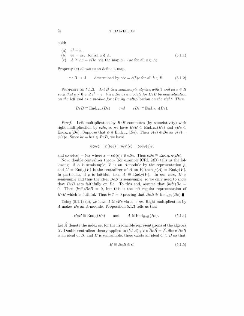
(6) Let ΞPn(x) denote the character table of the partition algebra Pn(x),that is the table of characters which has rows indexed by the irreduciblerepresentations and columns indexed by the elements described in (1). Us-ing our character formula and suitable orderings on the rows and columns,we see that

ΞPn(x) =

xΞPn−1(x)

... ∗· · · · · ·0

... ΞSn

, (0.1)

where ΞSn is the character table of Sn. Our rule allows us to efficientlycompute the values for ∗, and, in the lower-right corner of the table, itspecializes to the Murnaghan-Nakayama rule for Sn. We give charactertables for Pn(x) when n = 2, 3, 4, 5 in section 6.

(7) There is a natural embedding Pn−1(x) ⊆ Pn(x) which has specialproperties that are exploited by Martin [Ma3,4] to construct the irreduciblerepresentations of Pn(x). In section 5, we prove general results about thecharacters of algebras with these properties. In particular, Proposition5.1.9 tells us that the character table ΞPn(x) must have the form shown in(0.1). The Murnaghan-Nakayama rule is still needed, however, to directlycompute the entries from ∗.The general construction in section 5 holds for the rook monoid (see [Mu1,2],[So2]), the Solomon-Iwahori algebras ([So1], [So3], [Pu], [DHP]), and the“rook” version of the Brauer and Birman-Murakami-Wenzl algebras. Theconstruction is similar to the Jones basic construction, which is used in

4 T. HALVERSON

[HR] to compute the characters of the Temperley-Lieb, Brauer, Birman-Murakami-Wenzl, and Okada algebras.

ACKNOWLEDGMENTSThe bulk of this work was done during the Spring 1999 term at the Institute for

Advanced Study, whom I thank for their gracious hospitality. I thank Georgia Benkartand Arun Ram for listening to versions of this story and giving advice and Vahe Poladianfor implementing the character algorithms. I particularly thank Arun Ram for telling meabout the partition algebras and giving me encouragement and numerous suggestions.

1. PARTITION ALGEBRAS

In this section we give the combinatorial definition of the partition alge-bras and describe its irreducible representations using its duality with thesymmetric group on tensor space.

1.1. Integer Partitions and Symmetric FunctionsA composition λ of the positive integer n, denoted λ |= n, is a sequence of

nonnegative integers λ = (λ1, λ2, . . . , λt) such that |λ| = λ1 + · · ·+ λt = n.The composition λ is a partition, denoted λ ` n, if λ1 ≥ λ2 ≥ · · · ≥ λt.The length `(λ) is the number of nonzero parts of λ. Given two partitionsλ, µ, we say that µ ⊆ λ if µi ≤ λi for all i. If µ ⊆ λ, let λ/µ denotethe skew shape given by removing µ from λ. The size of a skew shape is|λ/µ| = |λ| − |µ|. The Young (or Ferrers) diagram of λ is the left-justifiedarray of boxes with λi boxes in the ith row. For example,

(5, 5, 3, 1) = (5, 5, 3, 1)/(3, 2, 1) =

Let mi(λ) denote the number of parts λi of λ which are equal to i. Wesometimes use the notation λ = (1m1(λ), 2m2(λ), . . .). In this notation thepartition above is given by (1, 3, 52).

For a positive integer k define the power symmetric function in the vari-ables x1, . . . , xr to be

pk(x1, . . . , xr) = xk1 + · · ·+ xkr ,

and for a partition µ define

pµ = pµ1pµ2 · · · pµ`(µ) .

For a partition λ ` r, a column strict tableau T of shape λ is a filling ofthe boxes of the Young diagram of λ with entries from {1, . . . , r} in such


a way that the entries in the columns strictly increase when read from topto bottom and the entries in the rows weakly increase when read from leftto right. For a column strict tableau T , let mi(T ) denote the number ofentries of T equal to i. The Schur function can be defined as

sλ(x1, . . . , xr) =∑T

xm1(T )1 x

m2(T )2 · · ·xmr(T )

r ,

where the sum is over all column strict tableaux of shape λ.

1.2. Set Partitions and Partition AlgebrasWe consider simple graphs on two rows of n-vertices, one above the other.

The connected components of such a graph partition the 2n vertices into kdisjoint subsets with 1 ≤ k ≤ 2n. We say that two diagrams are equivalentif they give rise to the same partition of the 2n vertices. For example, thefollowing are equivalent graphs.

∼•

•

•

•

•

•

•

•

•

•

•

•

•

•

•

•

........

........

........

........

........

........

........

........

.

.....................................................................................................

..........................................................................................................................................................................................................................

....................................................................................

..........................................................................

..........................................................................

..........................................................................

........

........

........

........

........

........

........

........

.

....................................

....................................

........

........

........

........

........

........

........

........

.

........

........

........

........

........

........

........

........

.

...................................................................................... •

•

•

•

•

•

•

•

•

•

•

•

•

•

•

•

........

........

........

........

........

........

........

........

..................................... ....................................

.....................................................................................................

......................................................................................................................................................................................

....................................................................................

..........................................................................

........

........

........

........

........

........

........

........

.

....................................

....................................

........

........

........

........

........

........

........

........

.

........

........

........

........

........

........

........

........

.

We will use the term partition diagram (or sometimes n-partition diagramto indicate the number of dots) to mean the equivalence class of the givengraph.

The number of n-partition diagrams which partition the 2n vertices intoexactly k subsets is the Stirling number S(2n, k), and the total number ofn-partition diagrams is the Bell number (see, for example, [Mac] I.2, ex.11)

B(2n) =2n∑k=1

S(2n, k). (1.2.1)

Let x be an indeterminate. We multiply two n-partition diagrams d1 andd2 as follows:

1. Place d1 above d2 and identify the vertices in the bottom row of d1

with the corresponding vertices in the top row of d2. This partition diagramnow has a top row, a bottom row, and a middle row.

2. Let γ denote the number of subsets in this new partition diagramwhich contain vertices only from the middle row.

3. Let d3 denote the n-partition diagram obtained by using only the topand bottom row (ignoring the middle row) with the imposed connections.(Note that we have removed the γ disjoint subsets that were only in themiddle row).

4. The product of d1 and d2 is then given by d1d2 = xγd3.

6 T. HALVERSON

For example,

•

•

•

•

•

•

•

•

•

•

•

•

•

•

•

•

•

•

................................................................................................

........

........

........

........

........

........

........

........

.....................................

.....................................................................................................

.............................................................................................................................................................................................................. ........

........

........

........

........

........

........

........

.

....................................

....................................

........

........

........

........

........

........

........

........

.

............................................................................................................................................

...........

............................

..........................................................................................

•

•

•

•

•

•

•

•

•

•

•

•

•

•

•

•

•

•

....................................

.................................... .....................................................................................................

.......................................................................... .......................................................................... .................................................................

....................................

....................................

....................................

...................................................................................................................

.............................................................................................................

.........................................................................................

......

= x2

•

•

•

•

•

•

•

•

•

•

•

•

•

•

•

•

•

•

......................................................................................................................................................................................................................

.....................................................................................................

.................................................................

.................................................................

....................................

............................................................................................................

..........................................................................................................

.

This product is associative and is independent of the graph that we chooseto represent the n-partition diagram.

Let C(x) be the field of rational functions with complex coefficients in anindeterminate x. The partition algebra Pn(x) is defined to be the C(x)-spanof the n-partition diagrams. Partition diagram multiplication makes Pn(x)into an associative algebra whose identity idn is given by the partitiondiagram having each vertex in the top row connected to the vertex belowit in the bottom row. The dimension of Pn(x) is the Bell number B(2n)(see (1.2.1)), and by convention P0(x) = C(x).

The Brauer algebra Bn(x) (see [Br]) is embedded in Pn(x) as the spanof the partition diagrams for which each edge is adjacent to exactly twovertices. The group algebra C(x)[Sn] of the symmetric group Sn is embed-ded in Pn(x) as the span of the partition partition diagrams for which eachedge is adjacent to exactly two vertices, one in each row.

For 1 ≤ i ≤ n− 1 and 1 ≤ j ≤ n, let

si =•

•

•

•

· · ·

· · ·

•

•

•

•

•

•

•

•

· · ·

· · ·

•

•i

........

........

........

........

........

........

........

........

.

........

........

........

........

........

........

........

........

.

........

........

........

........

........

........

........

........

.

........

........

........

........

........

........

........

........

.

........

........

........

........

........

........

........

........

.

..........................................................................

..........................................................................

,Ai =

•

•

•

•

· · ·

· · ·

•

•

•

•

•

•

•

•

· · ·

· · ·

•

•i

........

........

........

........

........

........

........

........

.

........

........

........

........

........

........

........

........

.

........

........

........

........

........

........

........

........

.

........

........

........

........

........

........

........

........

.

........

........

........

........

........

........

........

........

.

....................................

....................................

,

bi =•

•

•

•

· · ·

· · ·

•

•

•

•

•

•

•

•

· · ·

· · ·

•

•i

........

........

........

........

........

........

........

........

.

........

........

........

........

........

........

........

........

.

........

........

........

........

........

........

........

........

.

........

........

........

........

........

........

........

........

.

........

........

........

........

........

........

........

........

.

............................................

........

........

........

........

........

........

........

.

........

........

........

........

........

........

........

........

.....................................

,Ej =

•

•

•

•

· · ·

· · ·

•

•

•

•

•

•

•

•

· · ·

· · ·

•

•j

........

........

........

........

........

........

........

........

.

........

........

........

........

........

........

........

........

.

........

........

........

........

........

........

........

........

.

........

........

........

........

........

........

........

........

.

........

........

........

........

........

........

........

........

.................................................................. .

Notice that we have the relations

(a) A2i = xAi, (b) E2

j = xEj , (c) Ai = biEiEi+1bi. (1.2.2)

For 1 ≤ i ≤ n− 1 and 1 ≤ j ≤ n, we define

ai =1xAi and ej =

1xEj (1.2.3)


so that ai and ej are idempotent.The element si corresponds to the simple transposition si = (i, i+ 1) ∈

Sn, and the elements of the set {si | 1 ≤ i ≤ n−1} generate C(x)[Sn]. Theelements {si, Ai | 1 ≤ i ≤ n− 1} generate the Brauer algebra Bn(x).

The elements {si, bi, Ej | 1 ≤ i ≤ n − 1, 1 ≤ j ≤ n} generate all ofPn(x). To see this, think of a diagram d as living within the rectanglewhich has as its corners the vertices 1, n, n+ 1 and 2n. Following [Jo], wesay that a partition diagram d is planar if it is possible to draw a collectionof non-intersecting closed curves inside the rectangle of d which partitionthe vertices of d into its equivalence classes. It is then possible to writed = σpτ , where σ, τ ∈ Sn and p is a planar partition diagram (see [Jo],Lemma 2, for the obvious proof of this fact). For example, the diagram d2,above, decomposes as

••••••••••••••••...................................................................................................................

...................................................................................................................

...................................................................................

...................................................................................

........................................................

........................................................

........................................................

.......................................................................................................................................................................................

••••••••••••••••

=....................................

.................................... ...............................................................................

........................................................ ........................................................ ...........................................

....................................

....................................

...........................................

..................................................................................................................................................

....................................................................................................................................................................................

........... ••••••••••••••••.................................... ....................................

..............................

..............................

.......................

...........................................................................................................

...........................................

........................................................................

........

........

........

........

........

...

........

........

........

........

........

...

........................................................................

••••••••••••••••...........................................

...........................................

...........................................

........................................................

...................................................................................................................

...................................................................................

........................................................

........................................................

Now, it is easy to see that each planar partition diagram can be writtenas a product of bi, 0 ≤ i ≤ n− 1, and Ej , 0 ≤ j ≤ n. The planar diagramin our example can be written as

••••••••••••••••.................................... ....................................

..............................

..............................

.......................

...........................................................................................................

...........................................

........................................................................

........

........

........

........

........

...

........

........

........

........

........

...

........................................................................=

••••••••••••••••...........................................

...........................................

....................................

....................................

....................................

....................................

....................................

....................................

...........................................

...........................................

...........................................

...........................................

...........................................

••••••••••••••••...........................................

...........................................

...........................................

...........................................

...........................................

...........................................

....................................

....................................

••••••••••••••••...........................................

...........................................

...........................................

...........................................

...........................................

...........................................

...........................................

...........................................

....................................

....................................

••••••••••••••••...........................................

...........................................

...........................................

...........................................

...........................................

...........................................

...........................................

...........................................

....................................

....................................

It is well-known and easy to prove by induction that the number of planarpartition diagrams is the Catalan number 1

2n+1

(4n2n

). Moreover, the product

of two planar partition diagrams is planar, so the span of these diagramsis a subalgebra K(2n, x).

For each complex number ξ ∈ C, one defines a partition algebra Pn(ξ)over C as the linear span of n-partition diagrams where the multiplicationis as given above except with x replaced by ξ. The following theorem canbe proved using the same argument that Wenzl [Wz] uses for the Braueralgebra, only with the dimension of the irreducible Sr-module dim(Sλ) =

8 T. HALVERSON

r!/hλ replacing the El Samra-King polynomials. Here hλ is the product ofthe hooks in λ (see [Mac]).

Theorem 1.2.4. (Martin and Saleur [MS]) For each integer n ≥ 0,Pn(x) is semisimple over C(x), and Pn(ξ) is semisimple over C wheneverξ is not an integer in the range [0, 2n− 1].

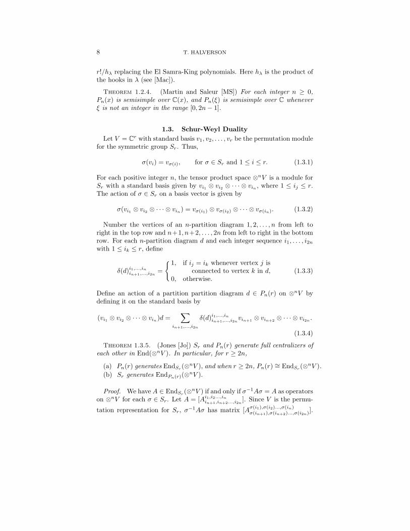
1.3. Schur-Weyl DualityLet V = Cr with standard basis v1, v2, . . . , vr be the permutation module

for the symmetric group Sr. Thus,

σ(vi) = vσ(i), for σ ∈ Sr and 1 ≤ i ≤ r. (1.3.1)

For each positive integer n, the tensor product space ⊗nV is a module forSr with a standard basis given by vi1 ⊗ vi2 ⊗ · · · ⊗ vin , where 1 ≤ ij ≤ r.The action of σ ∈ Sr on a basis vector is given by

σ(vi1 ⊗ vi2 ⊗ · · · ⊗ vin) = vσ(i1) ⊗ vσ(i2) ⊗ · · · ⊗ vσ(in). (1.3.2)

Number the vertices of an n-partition diagram 1, 2, . . . , n from left toright in the top row and n+1, n+2, . . . , 2n from left to right in the bottomrow. For each n-partition diagram d and each integer sequence i1, . . . , i2nwith 1 ≤ ik ≤ r, define

δ(d)i1,...,inin+1,...,i2n=

{ 1, if ij = ik whenever vertex j isconnected to vertex k in d,

0, otherwise.(1.3.3)

Define an action of a partition partition diagram d ∈ Pn(r) on ⊗nV bydefining it on the standard basis by

(vi1 ⊗ vi2 ⊗ · · · ⊗ vin)d =∑

in+1,...,i2n

δ(d)i1,...,inin+1,...,i2nvin+1 ⊗ vin+2 ⊗ · · · ⊗ vi2n .

(1.3.4)

Theorem 1.3.5. (Jones [Jo]) Sr and Pn(r) generate full centralizers ofeach other in End(⊗nV ). In particular, for r ≥ 2n,

(a) Pn(r) generates EndSr (⊗nV ), and when r ≥ 2n, Pn(r) ∼= EndSr (⊗nV ).(b) Sr generates EndPn(r)(⊗nV ).

Proof. We have A ∈ EndSr (⊗nV ) if and only if σ−1Aσ = A as operatorson ⊗nV for each σ ∈ Sr. Let A = [Ai1,i2...,inin+1,in+2...,i2n

]. Since V is the permu-

tation representation for Sr, σ−1Aσ has matrix [Aσ(i1),σ(i2)...,σ(in)σ(in+1),σ(in+2)...,σ(i2n)].


Hence the entries of the matrix of A are equal for all coordinates in theorbit of σ. If we collect the i1, i2, . . . , i2n according to those that have anequal value, we form a partition of {1, . . . , 2n} into subsets, and the indicesin each subset will always have equal value in an orbit of σ.

Given an equivalence relation ∼ which partitons the set {1, 2, . . . , 2n}into at most r subsets, define T∼ ∈ End(⊗nV ) by

[(T∼)i1,i2...,inin+1,in+2...,i2n] =

{1, if ij = ik whenever j ∼ k0, otherwise.

Then, the set T∼, as ∼ ranges over all partitions of {1, 2, . . . , 2n} intoat most r subsets, forms a basis of EndSr (⊗nV ). Moreover, this is ex-actly the matrix of the corresponding partition diagram (see 1.3.3). Whenr ≥ 2n, all equivalence relations∼ occur, and the representation of Pn(r) onEnd(⊗nV ) is faithful. Part (b) follows since these centralizer algebras aresemisimple and because Pn(r) is the centralizer of Sr.

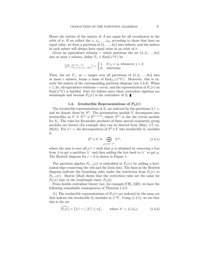
1.4. Irreducible Representations of Pn(r)The irreducible representations of Sr are indexed by the partitions λ ` r,

and we denote them by Sλ. The permutation module V decomposes intoirreducibles as V ∼= S(r) ⊕ S(r−1,1), where S(r) is the the trivial modulefor Sr. The rules for Kronecker products of these special symmetric groupmodules are known (for example they can be derived from [Mac], I.7, ex.23(d)). For λ ` r, the decomposition of Sλ⊗V into irreducible Sr modulesis

Sλ ⊗ V ∼=⊕

µ=(λ−)+

V µ, (1.4.1)

where the sum is over all µ ` r such that µ is obtained by removing a boxfrom λ to get a partition λ− and then adding the box back to λ− to get µ.The Bratteli diagram for r = 6 is shown in Figure 1.

The partition algebra Pn−1(x) is embedded in Pn(x) by adding a hori-zontal edge connecting the nth and the 2nth dots. The lines in the Brattelidiagram indicate the branching rules under the restriction from Pn(r) toPn−1(r). Martin [Ma4] shows that the restriction rules are the same forPn(x) and, in the semisimple cases, Pn(ξ).

From double centralizer theory (see, for example [CR], §3D), we have thefollowing remarkable consequences of Theorem 1.3.5:

(1) The irreducible representations of Pn(r) are indexed by the same setthat indexes the irreducible Sr-modules in ⊗nV . Using (1.4.1), we see thatthis is the set

Pn(r) ={λ ` r

∣∣ |λ∗| ≤ n} , where λ∗ = λ/(λ1). (1.4.2)

10 T. HALVERSON

P0(6) :......................................................

........................................................................................................................................

P1(6) :........................................................................

........................................................................................................................................

................................................................................................................................

......................................................

......................................................

............................................................................

................................................................................................................................................

P2(6) :.........................................................................................

..................................................................................................................................................

........................................................................................................................................

........................................................................

........................................................................

.........................................................................................

........................................................................................................................................................

.........................................................................................

........................................................................

........................................................................

............................................................................................................

....................................................................................................................................................................

.................................................................................................................................................................................................................................

....................................................................................................................................................................

.........................................................................................................

...............................................................

...............................................................

................................................................................................................................................

..............................................................................................................................................................................................................

P3(6) :

......

......

......

......

. . .

FIG. 1. The Bratteli diagram for Pn(6)

Here λ∗ is the partition obtained from λ by removing its first part λ1, i.e.,

λ =

........

........

........

........

........

........

........

........

........

........

........

........

........

........

........

........

........

.......

...................................................................................................................................

........

........

........

........

........

........

........

........

...................................................................................................................................................................................................................................................................................................................

....................................................................................................................................................................................................

........

........

........

........

....

........

........

........

........

....

λ1

λ∗

(2) Denote by Mλ the irreducible representation of Pn(r) indexed byλ ∈ Pn(r). The dimension of Mλ equals the multiplicity of Sλ in ⊗nV andthus is the number of paths from the top of the Bratteli partition diagramto λ. In row n = 3 of Figure 1, these dimensions are 5, 10, 6, 6, 1, 2, 1(reading left to right). Moreover, 52 + 102 + 62 + 62 + 12 + 22 + 1 = 203which is the Bell number B(6).

(3) The decomposition of ⊗nV as a bimodule for Sr × Pn(r) is

⊗nV ∼=⊕

λ∈Pn(r)

Sλ ⊗Mλ, (1.4.3)

and, when r ≥ 2n, {Mλ | λ ∈ Pn(r)} is a complete set of irreduciblePn(r)-modules.


Remark 1.4.4. We have two symmetric groups acting on ⊗nV . Thegroup Sr ⊆ GL(r,C) acts on the left by the tensor product of its permuta-tion representation, and the group Sn ⊆ Pn(r) acts on the right by tensorplace permutations.

Remark 1.4.5. In the classical case [Sc1,2], V = Cr is the standardrepresentation of GL(r,C) where g ∈ GL(r,C) acts by matrix multiplica-tion on the left. Restriction from GL(r,C) to Sr gives the permutationrepresentation (1.3.1) of Sr. The centralizer algebra is C[Sn] ⊆ Pn(r) withthe action given by (1.3.4). When r ≥ n,

⊗nV ∼=⊕λ`n

V λ ⊗ Sλ, (1.4.6)

where V λ is a GL(r,C)-module of highest weight λ and Sλ is an irreducibleSn-module.

1.5. Irreducible Representations of Pn(x)

When r ≥ 2n, the index set Pn(r) defined in (1.3.8) is in bijection withthe set

Pn = Pn(2n) = {λ ` 2n | |λ∗| ≤ n}. (1.5.1)

If λ ∈ Pn(r), the bijection is given by subtracting r − 2n from λ1. Sincer ≥ 2n and |λ∗| ≤ n, we see that λ1 − λ2 ≥ (r− n)− n = r− 2n, and thusthis subtraction will always give a partition of 2n.

Martin [Ma3] shows that, in the semisimple cases, the irreducible repre-sentations of Pn(x) and Pn(ξ) are indexed by the partitions µ ` k, 0 ≤ k ≤n. These partitions are also in bijection with Pn. Indeed, they are exactlythe partitions λ∗ in (1.5.1) and (1.4.2). We get from Martin’s partitions tothose in Pn by adding a top row with 2n − k boxes. The partitions in Pnare better suited for the recursive algorithm that we derive in section 4.

For λ ∈ Pn, let χλPn(ξ) denote the irreducible character of Pn(ξ) corre-sponding to Mλ. The proof of the next proposition is identical to that ofCorollary 2.4 in [Ra2].

Proposition 1.5.2. For all but a finite number of ξ ∈ C, the characterχλPn(ξ) of Pn(ξ) equals the character χλPn(x) of Pn(x) evaluated at x = ξ.

12 T. HALVERSON

2. CONJUGACY CLASS ANALOGS

In this section, we divide the partition algebra diagrams into classes onwhich characters are constant. These are analogs of the conjugacy classes,determined by cycle type, in the symmetric group.

2.1. Standard ElementsLet γ1 = 1, for t > 1 let γt = st−1st−2 · · · s1, and let E1 be the 1-partition

diagram with no edges. Thus,

γt =1 2 t•••••••· · ·

· · ·••••....................................................

....................................................

....................................................

..........................................................................................................

......................................................

......................................... and E1 =

••

(2.1.1)

If d1 and d2 are n1 and n2-partition diagrams respectively, then d1 ⊗ d2 isthe (n1 + n2)-partition diagram obtained by placing d2 to the right of d1.For µ = (µ1, · · · , µ`) |= k, define

γµ = γµ1 ⊗ · · · ⊗ γµ` ∈ Sk,

and for a composition µ with 0 ≤ |µ| ≤ n, define

dµ = γµ ⊗ E⊗(n−|µ|)1 = γµ ⊗ E1 ⊗ · · · ⊗E1︸︷︷︸

n−|µ| times

∈ Pn(x), (2.1.2)

The cycle type of a permutation σ ∈ Sn is the partition ρ(σ) ` n givenby the lengths of the disjoint cycles in σ. Each σ ∈ Sn is conjugate to γρ(σ),and { γρ | ρ ` n } is a complete set of Sn-conjugacy class representatives.

2.2. “Cycle Type” in the Partition Algebras.Let d ∈ Pn(x) be a partition diagram. The vertices of d are arranged

in n columns of size 2. Connect each vertex in d to the other vertex in itscolumn with a dotted line. The connected components of this new diagrampartition the vertices into disjoint subsets, called blocks. Vertices in thesame column are always in the same block, and there are no connectionsbetween disjoint blocks. The following diagram consists of four blocks.The first is on columns 1, 2, 3, 5, the second on columns 4, 6, 8, the third oncolumn 7, and the fourth on columns 9, 10.

1 2 3 4 5 6 7 8 9 10

•

•

•

•

•

•

•

•

•

•

•

•

•

•

•

•

•

•

•

•...

... ......

......

...

......

......

...

........

........

........

........

........

........

........

........

.

....................................

..........................................................................

..........................................................................................................................................................................

........

........

........

........

........

........

........

........

..............................................................................................................................................................

................................................................................................

................................................................................................ ....................................

....................................

........

........

........

........

........

........

........

........

.

........

........

........

........

........

........

........

........

.

......................................................................................

A vertex in d is isolated if is incident to no edges, and an an edge in d ishorizontal if it connects vertices in the same row. If a vertex is adjacent to


two vertices in the opposite row, then those two vertices are adjacent by ahorizontal edge. Thus, if d has no isolated vertices and no horizontal edges,then d ∈ Sn. Furthermore, a single block in an Sn diagram is a cycle.

We assign a nonnegative integer to each block, called the block type,using the following algorithm:

1. While the block is not E1 or a permutation diagram, do the following:

(i) If the block has an isolated vertex v, then remove the column con-taining v from the block (removing the edges incident to the other vertexin same column as v).

(ii) If the block has a horizontal edge, then

a. connect the corresponding vertices in the opposite row by an edgeb. add any new edges that are now implied by transitivityc. remove one of these two columns from the diagram.

2. If the remaining block is E1, then it has block type 0. Otherwise, theremaining block is a permutation diagram and so it is a cycle. The blocktype in this case is the length of this cycle, i.e., the number of columnsremaining in the block.

For example, we apply the algorithm to the first block in the exampleabove:

•

•

•

•

•

•

•

•

........

........

........

........

........

........

........

........

.

....................................

..........................................................................

....................................................................................................................................................

........

........

........

........

........

........

........

........

.....................................................................................................................................

......................................................................................

−→(i)

•

•

•

•

•

•

........

........

........

........

........

........

........

........

.

....................................

.......................................................................... .................................................................................................................................................................

......................................................................................

−→(ii)a

•

•

•

•

•

•

........

........

........

........

........

........

........

........

.

....................................

.......................................................................... .........................................................................................................................................................................................................................................

......................................................................................

−→(ii)b

•

•

•

•

•

•

........

........

........

........

........

........

........

........

.

....................................

....................................................................................................................................................

..........................................................................

..........................................................................

........

........

........

........

........

........

........

........

.....................................

............................................

........

........

........

........

........

........

........

.....................................

−→(ii)c

•

•

•

•

........

........

........

........

........

........

........

........

.

....................................

....................................................................................................................................................

........

........

........

........

........

........

........

........

.....................................

−→(ii)c

•

•

........

........

........

........

........

........

........

........

.

and this block has type 1.The sequence of block types of d forms a partition µ = (0m0 , 1m1 , . . .),

where mi is the number of blocks of type i. Note that

n− |µ| −m0 = (the number of columns removed in the algorithm).

In our example, the blocks have type 1, 3, 0, and 1, respectively, and so thethe block type of the diagram is (0, 12, 3). Here n = 10 and 10− 5− 1 = 4.Three columns were removed from the first block in the illustration above,and we remove 1 column when determining the type of the last block.

If d, d′ ∈ Pn(x), then we say that d′ is conjugate to d if there existsπ ∈ Sn such that d′ = πdπ−1. The following properties are easy to verify:

14 T. HALVERSON

1. If d is a partition diagram, then πdπ−1 is the partition diagram givenby rearranging the vertices of d, in both the top and bottom row, accordingto π.

2. If χ is any character of Pn(x), then χ(πdπ−1) = χ(d).3. d1 ⊗ d2 is conjugate to d2 ⊗ d1.4. π−1dπ has the same block type as d.5. If d ∈ Pn(x) has blocks of size k1 ≥ k2 ≥ . . . ≥ k`, then there exists

π ∈ Sn so that

π−1dπ = b1 ⊗ b2 ⊗ · · · ⊗ b`,

where each bi is consists of a single block of size ki in Pki(x). Simplychoose π to rearrange the vertices so that those in the largest block comefirst, those in the next largest block come next, and so on (breaking tiesarbitrarily).

6. Each cycle of length t is conjugate to γt.

Proposition 2.2.1. If d is a partition diagram with block type µ =(0m0 , 1m1 , . . .) and χ is any character of Pn(x), then

χ(d) = x−(n−|µ|−m0)χ(dµ),

where dµ = γµ ⊗ E⊗(n−|µ|)1 is a standard diagram defined in (2.1.2).

Proof. From 1-5 above, we see that we can work on the individual blocksof d independently, and thus we assume that d consists of a single block.If there is only one column in d, then we are done, since the two possiblepartition diagrams in this case are of the form (2.1.2). Thus, we assumethat d has more than 1 column.

(i) If d has an isolated vertex at position i in the top row, then the vertexbelow it is not isolated, since d is a block with more than one column. Thus

Eid = xd and dEi = d′

where d′ is the same diagram as d only the edges incident to the ith vertexin the bottom row have been removed. By permuting the ith column tothe end, d′ is conjugate to d′′ ⊗E1 where d′′ is the diagram obtained fromd by removing the ith column. Thus,

χ(d) =1xχ(Eid) =

1xχ(dEi) =

1xχ(d′′ ⊗ E1).

The symmetric argument is used when the isolated dot is in the bottomrow.


(ii) If d has a horizontal edge in the top row connecting vertices i and j,define

b = ••· · ·· · ·••••••· · ·· · ·••••••· · ·· · ·••

i j

........

........

........

........

........

...

........

........

........

........

........

...

........

........

........

........

........

...

........

........

........

........

........

...

........

........

........

........

........

...

........

........

........

........

........

...

........

........

........

........

........

...............................................................................................

.

Then

bd = d and db = d′

where d′ has an isolated vertex in the bottom row of the jth column. Nowcase (i) applies to get χ(d) = 1

xχ(d′ ⊗ E1) where d′ is obtained from d byconnecting the ith and jth vertices in the bottom row, connecting any newedges implied by transitivity, and then removing the jth column. Again,the symmetric argument is used for horizontal edges in the bottom row.

Each application of (i) or (ii) removes one column from the diagram andadds E1 at the end. Eventually we reach a permutation diagram (no iso-lated vertices and no horizontal edges), which is conjugate to a cycle γt, orwe reach E1. The argument is the same for Pn(ξ), ξ ∈ C, ξ 6= 0, only with ξreplacing x.

3. THE FROBENIUS FORMULA

For a partition λ ` r, let χλSr denote the irreducible character of thesymmetric group Sr corresponding to Sλ. If λ ` r and |λ∗| ≤ n (see(1.4.2)), then let χλPn(r) denote the irreducible character of the partitionalgebra Pn(r) corresponding to Mλ.

3.1. The Frobenius Formula for the Symmetric GroupAs in sections 1.3 and 1.4, let V = Cr be the natural representation of

GL(r,C), and let ⊗nV be its n-fold tensor product. Let Sn act on ⊗nV bythe action defined in (1.3.4). Define the bitrace of g × τ ∈ GL(r,C) × Snon ⊗nV to be

btr(g, τ) =∑

i1,...,in

g(vi1 ⊗ · · · ⊗ vin)τ∣∣vi1⊗···⊗vin

(3.1.1)

where g(vi1 ⊗· · ·⊗ vin)τ∣∣vi1⊗···⊗vin

denotes the coefficient of vi1 ⊗· · ·⊗ vinin the expansion of g(vi1⊗· · ·⊗vin)τ . Since the actions of GL(r,C) and Sncommute, the bitrace is a trace in both components, and thus it is sufficientto compute the bitrace on conjugacy class representatives.

For g ∈ GL(r,C) with eigenvalues x1, . . . , xr and γµ ∈ Sn with µ ` nas in (2.1.2), Schur [Sc1,2] proved that the bitrace is given by the power

16 T. HALVERSON

symmetric function,

btr(g, γµ) = pµ(x1, . . . , xr). (3.1.2)

The proof of (3.1.2) is a straight-forward computation (see [Ra2]). Theirreducible character of GL(r,C) corresponding to the highest weight mod-ule V λ is the Schur function sλ, so by computing the bitrace on both sidesof (1.4.6) we obtain Frobenius’ formula

pµ(x1, . . . , xr) =∑λ`n

sλ(x1, . . . , xr)χλSr (γµ). (3.1.3)

3.2. A Frobenius Formula for the Partition AlgebrasLet ρ ` r and µ |= m with 0 ≤ m ≤ n. Then let σ ∈ Sr, and let

dµ ∈ Pn(r) be defined as in (2.1.2). Since the actions of Sr and Pn(r)commute on ⊗nV , we define the bitrace of btr(σ, dµ) exactly as in (3.1.1)only with σ replacing g and dµ replacing γµ. Then, computing the traceon the right-hand side of (1.4.3) gives

btr(σ, dµ) =∑

λ∈Pn(r)

χλSr (σ)χλPn(r)(dµ) (3.2.1)

We now compute btr(σ, dµ) directly on ⊗nV .

Theorem 3.2.2. Let σ ∈ Sr and µ = (µ1, . . . , µ`) be a composition with0 ≤ |µ| ≤ n. The bitrace of σ × dµ ∈ Sr × Pn(r) on ⊗nV is given by

btr(σ, dµ) = rn−|µ|fµ(σ) = rn−|µ|fµ1(σ)fµ2(σ) · · · fµ`(σ)

where, if ρ = (ρ1, ρ2, . . .) is the cycle type of σ and k is a positive integer,then fk(σ) is computed by any of the following equivalent formulas:

(a) fk(σ) =∑`(ρ)i=1pk(1, ωρi , ω

2ρi , . . . , ω

ρi−1ρi ),

(b) fk(σ) =∑d|kd ·md(ρ), (summing over the divisors d of k),

(c) fk(σ) = χV (σk) = (the number of fixed points of σk),

such that ωj = e2πi/j is a primitive jth root of unity, md(ρ) is the num-ber of parts of ρ equal to d, and χV is the character of the permutationrepresentation V of Sr.

Proof. If σ ∈ Sr, d1 is an n1-partition diagram, and d2 is an n2-partitiondiagram, then btr(σ, d1⊗d2) = btr(σ, d1)btr(σ, d2) where σ×d1 acts on thefirst ⊗n1V and σ × d2 acts on the last ⊗n2V . It follows from (2.1.2) that

btr(σ, dµ) = btr(σ, γµ1)btr(σ, γµ2) · · · btr(σ, γµ`)btr(σ,E1)n−|µ|.


We compute the value of btr(σ,E1) on V directly. From (1.3.4), we seethat viE1 =

∑rj=1 vj , and thus

btr(σ,E1) =r∑i=1

σviE1|vi =r∑i=1

r∑j=1

σvj |vi =r∑i=1

r∑j=1

vσ(j)|vi =r∑i=1

1 = r.

Define fk(σ) = btr(σ, γk), and we have proved

fµ(σ) = rn−|µ|fµ1(σ) · · · fµ`(σ).

It remains to compute fk(σ).(a) Using Schur’s result (3.1.2) restricted to Sr ⊆ GL(r,C), we have

btr(γρ, γk) = pk(x1, . . . , xr),

where x1, . . . , xr are the eigenvalues of γρ. The eigenvalues of a j-cyclein Sr are the jth roots of unity 1, ωj , . . . , ω

j−1j , and σ ∈ Sr is a disjoint

product of cycles. Thus, the eigenvalues of σ ∈ Sr are the union of thejth roots of unity as j ranges over the lengths of the cycles in σ. Part (a)then follows from the fact that pk(x1, . . . , xa, y1, . . . , yb) = pk(x1, . . . , xa)+pk(y1, . . . , yb).

(b) If ωj = e2πi/j , then

pk(1, ωj , . . . , ωj−1j ) = 1 + ωkj + ω2k

j + · · ·+ ωk(j−1)j

=ωkjj − 1

ωkj − 1

={j, if j divides k,0, otherwise.

Thus, the only nonzero summands which appear in (a) are when ρi dividesk, and in that case the value is ρi. We can then sum the divisors d of k,and they appear with multiplicity md(ρ).

(c) The character value χV (σk) is the number of fixed points of σk, andthe fixed points of σk are the elements of the d-cycles of σ where d divides k.Part (c) then follows from from (b).

Putting (3.2.1) and Theorem 3.2.2 together gives our Frobenius formulafor the characters of Pn(r). For a composition µ with 0 ≤ |µ| ≤ n, we have

rn−|µ|fµ(σ) =∑

λ∈Pn(r)

χλPn(r)(dµ)χλSr (σ), for all σ ∈ Sr. (3.2.3)

18 T. HALVERSON

For each composition µ, the function fµ is a class function on Sr. LetR(Sr) denote the C-vector space generated by the class functions of Sr.The irreducible characters of Sr form a basis of R(Sr), and the Frobeniusformula (3.2.3) says that the character χλPn(r)(dµ) is the coefficient of χλSrwhen rn−|µ|fµ is expanded in terms of the irreducible Sr characters.

The module R(Sr) carries a scalar product 〈, 〉 which is defined by

〈g, h〉 =∑ρ`r

1zρg(γρ)h(γρ), for g, h ∈ R(Sr), (3.2.4)

where zρ =∏`(ρ)i=1 i

mi(ρ)mi(ρ)! is the size of the centralizer of γρ in Sr. Withrespect to this product the irreducible characters of Sr are orthonormal,and so we have the following corollary of our Frobenius formula.

Corollary 3.2.5. Let µ be a composition with 0 ≤ |µ| ≤ n, and letλ ` r with |λ∗| ≤ n. Then

χλPn(r)(dµ) = 〈rn−|µ|fµ, χλSr 〉 = rn−|µ|〈fµ, χλSr 〉.

4. THE MURNAGHAN-NAKAYAMA RULE

The Murnaghan-Nakayama rule is a recursive rule for computing char-acters of the symmetric group. It is derived by expanding polynomials inthe ring of symmetric functions. In our work here, we must derive the ruleby working in the character ring of the symmetric group.

4.1. The Murnaghan-Nakayama Rule for the Symmetric GroupTwo boxes in a skew shape λ/µ are adjacent if they share a common

edge, and λ/µ is connected if you can travel from any box to any othervia a path of adjacent boxes. A skew shape λ/µ is a border strip if it isconnected and it does not contain any 2× 2 blocks of boxes. The followingfigures illustrate the three border strips of size 4 in λ = (4, 4, 3, 1).

∗∗ ∗ ∗

∗ ∗∗ ∗

∗ ∗∗

∗

The height of a border strip is given by

ht(λ/µ) = #(rows occupied by λ/µ)− 1.


The heights of the border strips in the figures above are 1, 1, and 2, re-spectively. For a proof of the next theorem, see [Mac] I.7, ex. 5.

Theorem 4.1.1. (The Murnaghan-Nakayama Rule for Sn) Let λ ` n,µ |= n, and let µ be obtained from µ by removing a part of size k. Thenthe irreducible character χλSn(γµ) is given by

χλSn(γµ) =∑

λ−k⊆λ(−1)ht(λ/λ

−k)χλ−k

Sn−k(γµ),

where sum is over all partitions λ−k ⊆ λ such that λ/λ−k is a border stripof size k.

4.2. A Murnaghan-Nakayama Rule for the Partition AlgebrasIf χδSr is a character of Sr, and k is a positive integer, then fkχ

δSr

isthe class function which takes the value fk(σ)χδSr (σ) on σ ∈ Sr. Thenext proposition gives the expansion of fk(σ)χδSr (σ) in terms of the basisof irreducible characters. It is the analogue of the symmetric functionidentities [Mac], I.3 ex. 11(2), for the symmetric group and [Ra2], Theorem6.8, for the Brauer algebra.

Proposition 4.2.1. Let δ, λ ` r. Using the inner product 〈, 〉 on Srcharacters (3.2.4), we have

〈fkχδSr , χλSr 〉 =

∑d|k

∑λ−d⊆λλ−d⊆δ

(−1)ht(λ/λ−d)(−1)ht(δ/λ

−d)

where the outer sum is over all divisors d of k and the inner the sum isover all partitions λ−d ` (r − d) such that λ−d ⊆ λ, λ−d ⊆ δ and λ/λ−d

and δ/λ−d are border strips of size d. If no such λ−d exists, then the innerproduct is zero.

Proof. By (3.2.4) and Theorem 3.2.2, we have


∑ρ`r

1zρfk(ρ)χδSr (γρ)χ

λSr (γρ)

=∑d|k

∑ρ`r

dmd(ρ)zρ

χδSr (γρ)χλSr (γρ).

The nonzero terms of the inner sum occur when ρ ` r has at least onepart of size d. These partitions are in bijection with partitions of the formα + (d), where α ` (n − d) and α + (d) is the partition of r obtained byadding a part of size d to α. Moreover, for partitions of this form, we have

20 T. HALVERSON

zα+(d) = dmd(α+ (d))zα (see (3.2.4)), which implies that

dmd(α+ (d))zα+(d)

=1zα.

Thus,


∑d|k

∑α`(r−d)

1zαχδSr (γα+(d))χλSr (γα+(d)).

We now apply the Murnaghan-Nakayama rule for Sr (Theorem 4.1.1) toremove a part of size d from χδSr (γα+(d)) and χλSr (γα+(d)):


=∑d|k

∑α`(r−d)

1zα

∑δ−d⊆δ

∑λ−d⊆λ

(−1)ht(δ/δ−d)(−1)ht(λ/λ

−d)χδ−d

Sr−d(γα)χλ−d

Sr−d(γα)

=∑d|k

∑δ−d⊆δ

∑λ−d⊆λ

(−1)ht(δ/δ−d)(−1)ht(λ/λ

−d)∑

α`(r−d)

1zαχδ−d

Sr−d(γα)χλ−d

Sr−d(γα).

By orthogonality of Sr−d characters, the inner-most sum is equal to〈χδ−dSr−d

, χλ−d

Sr−d〉 = δδ−d,λ−d , where δδ−d,λ−d is a Kronecker delta. Thus, we

must have λ−d = δ−d to get a nonzero inner product, and the proposition isproved.

The following theorem is our analogue of the Murnaghan-Nakayama rule.For a partition λ, recall the definition of λ∗ in (1.4.2). Since we will beusing recursion on the n, we will sometimes add the subscript n to thedefinition of dµ from (2.1.2)

dµ,n = dµ = γµ ⊗ E⊗n−|µ|1 , where µ |= n.

Theorem 4.2.2. Let λ ` r with |λ∗| ≤ n. Let µ be a composition with0 ≤ |µ| ≤ n, and let µ be the composition obtained from µ by removing apart of size k. Then

χλPn(r)(dµ,n) =∑d|k

∑δ=(λ−d)+d

|δ∗|≤n−k

(−1)ht(λ/λ−d)(−1)ht(δ/λ

−d)χδPn−k(r)(dµ,n−k),

where the outer sum is over all divisors d of k and the inner sum is overall δ ` r with |δ∗| ≤ n − k such that δ is obtained from λ by removing aborder strip of size d to obtain the partition λ−d and then adding a borderstrip of size d to λ−d to obtain δ = (λ−d)+d.


Proof. Since µ |= (n − k), our Frobenius formula (3.2.3) gives thefollowing identity in R(Sr):

r(n−k)−|µ|fµ =∑δ`r

|δ∗|≤n−k

χδPn−k(r)(dµ,n−k)χδSr .

Using Proposition 4.2.1 and Corollary 3.2.5, we have

χλPn(r)(γµ) = 〈rn−|µ|fµ, χλSr 〉= 〈r(n−k)−|µ|fµfk, χ

λSr 〉

=∑δ`r

|δ∗|≤n−k

χδPn−k(r)(dµ,n−k)〈χδSrfk, χλSr 〉.

=∑δ`r

|δ∗|≤n−k

χδPn−k(r)(dµ,n−k)∑d|k

∑λ−d⊆λλ−d⊆δ

(−1)ht(λ/λ−d)(−1)ht(δ/λ

−d)

=∑d|k

∑δ=(λ−d)+d

|δ∗|≤n−k

(−1)ht(λ/λ−d)(−1)ht(δ/λ

−d)χδPn−k(r)(dµ,n−k).

The last equality follows from changing the order of summation and ob-serving that the inner product 〈χδSrfk, χλSr 〉 is zero unless δ can be ob-tained from λ by removing and then adding back a border strip of size d.

Corollary 4.2.3. If λ ` r with |λ∗| ≤ n and µ is a composition with0 ≤ |µ| ≤ n, then

(a) χλPn(r)(dµ) ={rn−|µ|χλP|µ|(r)(γµ), if |µ| ≥ |λ∗|,0, if |µ| < |λ∗|.

(b) if |µ| = |λ∗| = n, then χλPn(r)(dµ) = χλ∗

Sn(γµ).

(c) If r ≥ 2n and |µ| = n, then χλPn(r)(dµ) is independent of r.

Proof. (a) In P|µ|(r), we have dµ = γµ. If |µ| ≥ |λ∗|, then

χλPn(r)(dµ) = 〈rn−|µ|fµ, χλSr 〉 = rn−|µ|〈fµ, χλSr 〉 = rn−|µ|χλP|µ|(r)(γµ).

where the first and the third equality follow from Corollary 3.2.5.If |µ| < |λ∗|, then we recursively apply Theorem 4.2.2 until we have

removed all of the parts of µ. We are left with a sum of characters of theform

χδPn−|µ|(r)(E⊗(n−|µ|)1 ) = 〈rn−|µ|, χδSr 〉 =

{rn−|µ|, if δ = (r),0, otherwise,

22 T. HALVERSON

where the first equality comes from Corollary 3.2.5 and the second equalitycomes from the fact that the only character that is constant on all Srconjugacy classes is the trivial character χ(r)

Srwhich is 1 on all conjugacy

classes. The partitions δ have minimal |δ∗|, if at each step in the recursionwe remove a strip of size µi from δ∗ and add it to the first row of δ. Inthis case, we will have removed |µ| boxes from λ∗ to obtain δ∗. However,|λ∗| > |µ|, so |δ∗| > 0. In particular δ 6= (r), and so the above inner productis 0 for each summand.

For (b), note that in Theorem 4.2.2, if λ ` n, then when we remove andadd a border strip of size d|k from λ to obtain δ, we must have |δ∗| ≤ n−k.We are thus forced to remove a border strip of size k from λ−d and place itat the end of the first row in δ. The strip we add to δ has weight 1, and sowe only consider the weight of removing a border strip of size k from λ−d.This is precisely the Murnaghan-Nakayama rule for Sn (Theorem 4.1.1).

For (c) we see that if |µ| = n, then by (a) we have χλPn(r)(dµ) =χλPn(r)(γµ). If λ ` r with |λ∗| = n− `, then since r ≥ 2n, we have

λ1 − λ2 ≥ r − (n− `)︸︷︷︸λ1

− (n− `)︸︷︷︸≥λ2

= r − 2n+ 2` ≥ 2`,

so a border strip in λ that contains boxes from λ1 and λ2 has at least 2`+2boxes.

Suppose that d divides k and that we remove a border strip of size dfrom λ and add it back to obtain δ, with |δ∗| ≤ n − k. Assume that theborder strip that we remove contains boxes from both λ1 and λ2. If k ≥ `,then we must move at least k − ` boxes from λ∗ up to the first row of δ.But then d = (#boxes removed from λ∗) + (#boxes removed from λ1) ≥(k − `) + (2` + 1) = k + ` + 1 > k, a contradiction since d divides k. Onthe other hand, if ` > k, then d ≥ λ1 − λ2 ≥ 2` > k, also a contradiction.Thus, we can not remove a strip from λ that contains boxes from both λ1

and λ2, and in particular, we remove strips from λ1 and λ∗ independently.An entirely similar argument shows that we can never add back a strip of

size d that lives in both δ1 and δ∗. As r ≥ 2n varies, the set of possible λ∗ re-mains constant, only the length of the first row varies. Moreover, when r ≥2n, there is only one way to remove or add a strip of size d from or to the firstrow.

Now we use Corollary 4.2.3 to lift our character formula to Pn(x).

Theorem 4.2.4. Let λ ` r with |λ∗| ≤ n. Let µ be a composition with0 ≤ |µ| ≤ n, and let µ be the composition obtained from µ by removing apart of size k. Then


(a) if |µ| < n, then χλPn(x)(dµ) ={xn−|µ|χλP|µ|(γµ), if |µ| ≥ |λ∗|,0, if |µ| < |λ∗|.

(b) if |µ| = n, then dµ = γµ, and

χλPn(x)(γµ) =∑d|k

∑δ=(λ−d)+d

|δ∗|≤n−k

(−1)ht(λ/λ−d)(−1)ht(δ/λ

−d)χδPn−k(x)(γµ),

where the outer sum is over all divisors d of k and the inner sum is overall δ ` r with |δ∗| ≤ n − k such that δ is obtained from λ by removing aborder strip of size d to obtain the partition λ−d and then adding a borderstrip of size d to λ−d to obtain δ = (λ−d)+d.

Proof. Define fλµ(x) = 0 if |µ| < |λ∗|, and define

fλµ(x) = xn−|µ|∑d|k

∑δ=(λ−d)+d

(−1)ht(λ/λ−d)(−1)ht(δ/λ

−d)χδP|µ|−k(x)(γµ),

if |µ| < |λ∗|. Then, by Corollary 4.2.3, for r ≥ 2n we have fλµ(r) =χλPn(r)(dµ). For an infinite number of r ∈ Z, we have

fλµ(r) = χλPn(r)(dµ) = χλPn(x)(dµ)|x=r.

Since both fλµ(x) and χλPn(x)(dµ) are rational functions in x which agree atan infinite number of points, then by Proposition 1.5.2 they must be equaleverywhere.

5. BASIC CONSTRUCTION

To construct irreducible representations of Pn(x), Martin [Ma3] exploitsthe properties of P0(x) ⊆ P1(x) ⊆ P2(x) ⊆ · · · as a tower of semisimplealgebras. In this section, we derive general results about the charactersof algebras which have these basic properties. Other algebras of this formare the rook algebra ([Mu1,2], [So2]) and its Iwahori-Hecke algebra ([So1],[So3], [Pu]) and the “rook” versions of the Brauer and Birman-Murakami-Wenzl centralizer algebras. Frobenius formulas and Murnaghan-Nakayamarules for the rook monoid and its Iwhahori-Hecke algebra are determinedin [DHP].

5.1. Basic ConstructionLet A ⊆ B be an inclusion of finite-dimensional, semisimple algebras

with 1 over C. Let 0 6= e ∈ B, and assume that the following properties

24 T. HALVERSON

hold:

(a) e2 = e,(b) ea = ae, for all a ∈ A,(c) A ∼= Ae = eBe via the map a 7→ ae for all a ∈ A;

(5.1.1)

Property (c) allows us to define a map,

ε : B → A determined by ebe = ε(b)e for all b ∈ B. (5.1.2)

Proposition 5.1.3. Let B be a semisimple algebra with 1 and let e ∈ Bsuch that e 6= 0 and e2 = e. View Be as a module for BeB by multiplicationon the left and as a module for eBe by multiplication on the right. Then

BeB ∼= EndeBe(Be) and eBe ∼= EndBeB(Be).

Proof. Left multiplication by BeB commutes (by associativity) withright multiplication by eBe, so we have BeB ⊆ EndeBe(Be) and eBe ⊆EndBeB(Be). Suppose that ψ ∈ EndBeB(Be). Then ψ(e) ∈ Be so ψ(e) =ψ(e)e. Since be = be1 ∈ BeB, we have

ψ(be) = ψ(bee) = beψ(e) = beeψ(e)e,

and so ψ(be) = bex where x = eψ(e)e ∈ eBe. Thus eBe ∼= EndBeB(Be).Now, double centralizer theory (for example [CR], §3D) tells us the fol-

lowing: if A is semisimple, V is an A-module by the representation ρ,and C = EndA(V ) is the centralizer of A on V, then ρ(A) = EndC(V ).In particular, if ρ is faithful, then A ∼= EndC(V ). In our case, B issemisimple and thus the ideal BeB is semisimple, so we only need to showthat BeB acts faithfully on Be. To this end, assume that (beb′)Be =0. Then (beb′)BeB = 0, but this is the left regular representation ofBeB which is faithful. Thus beb′ = 0 proving that BeB ∼= EndeBe(Be).

Using (5.1.1) (c), we have A ∼= eBe via a 7→ ae. Right multiplication byA makes Be an A-module. Proposition 5.1.3 tells us that

BeB ∼= EndA(Be) and A ∼= EndBeB(Be). (5.1.4)

Let X denote the index set for the irreducible representations of the algebraX. Double centralizer theory applied to (5.1.4) gives BeB = A. Since BeBis an ideal of B, and B is semisimple, there exists an ideal C ⊆ B so that

B ∼= BeB ⊕ C (5.1.5)


and thus

B = A t C, (5.1.6)

where t denotes a disjoint union.

Lemma 5.1.7. If χ is a character of BeB, then χ is completely deter-mined by the values χ(ae) where a ∈ A.

Proof. (cf., [HR] Lemma 2.8). If b1eb2 ∈ BeB, then from the trace prop-erty of χ and the map ε defined in (5.1.2), we have χ(b1eb2) = χ(b1eeb2) =χ(eb2b1e) = χ(ε(b2b1)e)).

Lemma 5.1.8. If Q is a set of minimal orthogonal idempotents for A,then eQ = { eq | q ∈ Q} is a set of minimal orthogonal idempotents for B.Moreover, q is a minimal idempotent of A corresponding to λ ∈ A if andonly if eq is a minimal idempotent of B corresponding to λ ∈ A.

Proof. The proof of the first statement uses (5.1.1) (c) and the mapε defined in (5.1.2). We have (eq)2 = e2q2 = eq, and for q 6= q′ ∈ Q,eqeq′ = eeqq′ = 0. If b ∈ B, then (eq)b(eq) = q(ebe)q = qε(b)eq =qε(b)qe = αqqe = α(eq), for some scalar α, so eq is minimal.

Let zλ be a minimal central idempotent of A such that qzλ 6= 0. SinceA ∼= eBe via the isomorphism a 7→ ae, we have qzλe 6= 0. By the factthat A and BeB are full centralizers on Be, their centers coincide, andthus there is a minimal central idempotent z∗λ in BeB which acts by leftmultiplication on Be the same way that zλ acts on the right. In particular,0 6= qzλe = qezλ = z∗λqe, which shows that qe corresponds to λ ∈ B.

Proposition 5.1.9. If λ ∈ B and a ∈ A, then

χλB(ae) ={χλA(a), if λ ∈ A,0, if λ ∈ B \ A.

Proof. (cf., [HR] Proposition 2.10). Let P be a complete set of minimalorthogonal idempotents of A. Then 1 =

∑p∈P p. For a ∈ A, we have

ae =(∑p∈P

p)ae( ∑p′∈P

p′)

=∑p,p′∈P

paep′ =∑p,p′∈P

(ep)a(ep′) (5.1.10)

Using Lemma 5.1.8, extend eP to a complete set Q of minimal orthogonalidempotents of B. For b ∈ B and q ∈ Q, let b|q denote the coefficient ofq when b is expanded in terms of Q. Let Qλ denote the elements of Qcorresponding to the irreducible component of B indexed by λ (define Pλ

26 T. HALVERSON

similarly for A). Using (5.1.10), we have

χλB(ae) =∑q∈Qλ

(qaeq)|q =∑q∈Qλ

∑p,p′∈P

q(ep)a(ep′)q|q

Since q, ep ∈ Q, we have q(ep) = (ep)q ={ep, if ep = q,0, otherwise. Moreover,

ep ∈ Qλ if and only if p ∈ Pλ by Lemma 5.1.8, so

χλB(ae) =∑p∈Pλ

(ep)a(ep)|ep =∑p∈Pλ

pap|p = χλA(a)

as desired.

Let ΞB denote the character table for B, that is the table which hasrows indexed by B and columns indexed by appropriate basis elements ofB whose character values are sufficient to determine the characters of B.Proposition 5.1.8 tells us that we can order the rows and columns of ΞB sothat it takes the form

ΞB =

ΞA... ∗

· · · · · ·0

... ΞC

, (5.1.11)

where ΞC is the character table of C.

5.2. Application to the Partition AlgebrasThere is a natural inclusion

Pn−1(x) ⊆ Pn(x) (5.2.1)

given by adding a horizontal edge at the right end of the partition diagramof d ∈ Pn−1(x). Let en = 1

xEn. Then it can be readily checked by drawingdiagrams that e2

n = en and ena = aen for all a ∈ Pn−1(x). Furthermore,

Pn−1(x) → enPn(x)ena 7→ aen

(5.2.2)

is an algebra isomorphism. Thus, Pn−1(x) ⊆ Pn(x) satisfies our properties(5.1.1) of a basic construction.

For a partition diagram d, we follow Martin [Ma4] and define the prop-agating number, #(d) to be the number of distinct parts of d containingelements from both the top and bottom row of d. Then if d1, d2 are parti-tion diagrams, we have

#(d1d2) ≤ min(#(d1),#(d2)).


The ideal Pn(x)enPn(x) is spanned by all the diagrams having a propagat-ing number strictly less than n. Moreover, we have ([Ma3])

Pn(x) ∼= Pn(x)enPn(x)⊕ C[Sn]. (5.2.3)

It follows from (5.1.5) or directly from the definition (1.4.1) that theindex set Pn for the irreducible representations of Pn(r) is a disjoint union

Pn = Pn−1 t Sn. (5.2.4)

From Lemma 5.1.7 we know that if λ ∈ Pn−1, then χλ is completely deter-mined by the values χλ(aen) for a ∈ Pn−1(x). Moreover, by Proposition5.1.9, if λ ∈ Pn and a ∈ Pn−1(x), then

χλPn(x)(aen) ={χλPn−1(x)(a), if |λ∗| < n,0, if |λ∗| = n.

(5.2.5)

The character table ΞPn(x) has the form of (0.1). We see this in the exam-ples in section 6.

6. CHARACTER TABLES

The following tables give the characters of Pn(x) for n = 2, 3, 4, 5. Theentries in the tables are χλPn(x)(dµ). The rows of the tables are index theirreducible representations by the partitions λ∗ defined in (1.4.2), and thecolumns of the table are indexed by the partitions µ, which correspondto the standard element dµ defined in (2.1.2). The tables for Pn−1(x) isembedded in the table for Pn(x) according to (0.1), and so to save spacewe only give the rightmost part, where |µ| = n, of the tables for n = 4 andn = 5. The tables for Pn(r), r ≥ n, are obtained by setting x = r.

TABLE 1.

Characters of P2(x)

∅ (1) (2) (12)

∅ x2 x 2 2

(1) 0 x 1 3

(2) 0 0 1 1

(12) 0 0 −1 1

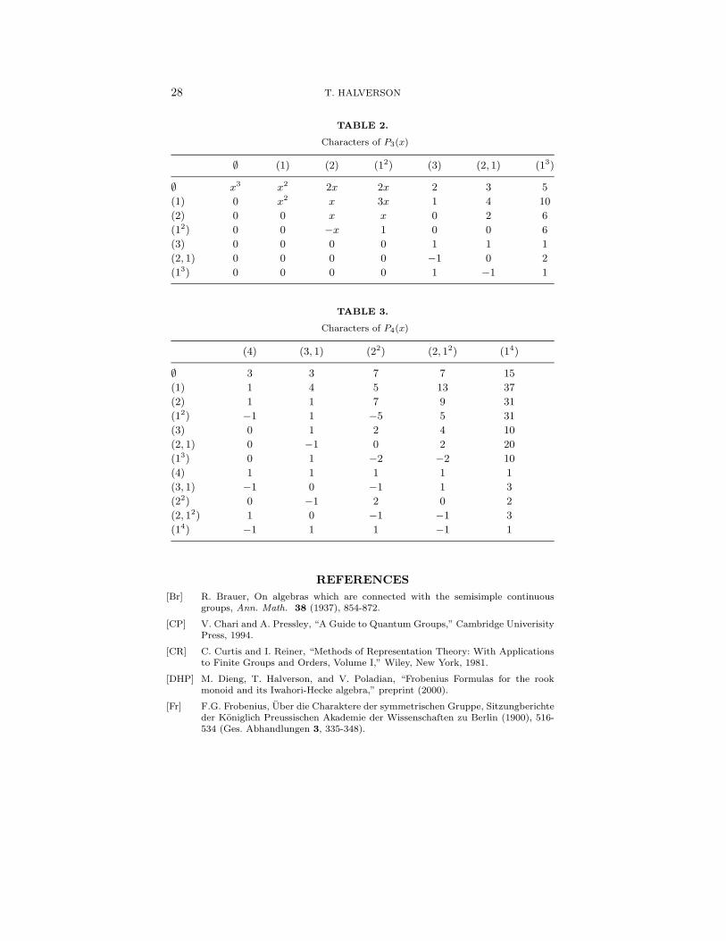
28 T. HALVERSON

TABLE 2.

Characters of P3(x)

∅ (1) (2) (12) (3) (2, 1) (13)

∅ x3 x2 2x 2x 2 3 5

(1) 0 x2 x 3x 1 4 10

(2) 0 0 x x 0 2 6

(12) 0 0 −x 1 0 0 6

(3) 0 0 0 0 1 1 1

(2, 1) 0 0 0 0 −1 0 2

(13) 0 0 0 0 1 −1 1

TABLE 3.

Characters of P4(x)

(4) (3, 1) (22) (2, 12) (14)

∅ 3 3 7 7 15

(1) 1 4 5 13 37

(2) 1 1 7 9 31

(12) −1 1 −5 5 31

(3) 0 1 2 4 10

(2, 1) 0 −1 0 2 20

(13) 0 1 −2 −2 10

(4) 1 1 1 1 1

(3, 1) −1 0 −1 1 3

(22) 0 −1 2 0 2

(2, 12) 1 0 −1 −1 3

(14) −1 1 1 −1 1

REFERENCES[Br] R. Brauer, On algebras which are connected with the semisimple continuous

groups, Ann. Math. 38 (1937), 854-872.

[CP] V. Chari and A. Pressley, “A Guide to Quantum Groups,” Cambridge UniverisityPress, 1994.

[CR] C. Curtis and I. Reiner, “Methods of Representation Theory: With Applicationsto Finite Groups and Orders, Volume I,” Wiley, New York, 1981.

[DHP] M. Dieng, T. Halverson, and V. Poladian, “Frobenius Formulas for the rookmonoid and its Iwahori-Hecke algebra,” preprint (2000).

[Fr] F.G. Frobenius, Uber die Charaktere der symmetrischen Gruppe, Sitzungberichteder Koniglich Preussischen Akademie der Wissenschaften zu Berlin (1900), 516-534 (Ges. Abhandlungen 3, 335-348).


TABLE 4.

Characters of P5(x)

(5) (4, 1) (3, 2) (3, 12) (22, 1) (2, 13) (15)

∅ 2 4 5 7 12 20 52

(1) 1 5 5 13 19 47 151

(2) 0 2 3 7 16 42 160

(12) 0 0 −1 7 0 32 160

(3) 0 1 3 3 11 21 75

(2, 1) 0 0 −2 0 2 22 150

(13) 0 −1 1 3 −9 1 75

(4) 0 1 1 3 3 7 15

(3, 1) 0 −1 0 0 1 9 45

(22) 0 0 −1 −3 2 2 30

(2, 11) 0 1 0 0 −3 −3 45

(14) 0 −1 1 3 −1 −5 15

(5) 1 1 1 1 1 1 1

(4, 1) −1 0 −1 1 0 2 4

(3, 2) 0 −1 1 −1 1 1 5

(3, 12) 1 0 0 0 −2 0 6

(22, 1) 0 1 −1 −1 1 −1 5

(2, 13) −1 0 1 1 0 −2 4

(15) 1 −1 −1 1 1 −1 1

[HR] T. Halverson and A. Ram, Characters of algebras containing a Jones basic con-struction: the Temperley-Lieb, Okada, Brauer, and Birman-Wenzl algebras, Adv.Math. 116 (1995), 263–321.

[Jo] V. F. R. Jones, The Potts model and the symmetric group in “Subfactors: Pro-ceedings of the Taniguchi Symposium on Operator Algebras (Kyuzeso, 1993),”World Sci. Publishing, River Edge, NJ, 1994, 259–267.

[Mac] I. G. Macdonald, “Symmetric functions and Hall polynomials,” Second edition,Oxford University Press, New York, 1995.

[MS] P. Martin and H. Saleur, On an algebraic approach to higher-dimensional statis-tical mechanics, Comm. Math. Phys. 158 (1993), 155–190.

[Ma1] P. Martin, Representations of graph Temperley-Lieb algebras, Publ. RIMS KyotoUniv. 26 (1990), 485–503.

[Ma2] P. Martin, “Potts models and related problems in statistical mechanics,” WorldScientific, Singapore, 1991.

[Ma3] P. Martin, Temperley-Lieb algebras for nonplanar statistical mechanics—the par-tition algebra construction, J. Knot Theory Ramifications 3 (1994), 51–82.

[Ma4] P. Martin, The structure of the partition algebras, J. Algebra 183 (1996), 319-358.

[MW1] P. Martin and D. Woodcock, The partition algebras and a new deformation ofthe Schur algebras, J. Algebra 203 (1998), 91-124.

30 T. HALVERSON

[MW2] P. Martin and D. Woodcock, On Central idempotents in the partition algebra, J.Algebra 217 (1999), 156-169.

[Mu1] W. D. Munn, Matrix representations of semigroups, Proc. Cambridge Philos. Soc.53 (1957), 5–12.

[Mu2] W. D. Munn, The characters of the symmetric inverse semigroup, Proc. Cam-bridge Philos. Soc. 53 (1957), 13–18.

[Pu] M. Putcha, Monoid Hecke algebras, Trans. Amer. Math. Soc. 349 (1997), 3517–3534.

[Ra1] A. Ram, A Frobenius formula for the characters of the Hecke Algebras, Invent.Math. 106 (1991), 461-488.

[Ra2] A. Ram, Characters of Brauer’s centralizer algebras, Pacific J. Math. 169 (1995),173–200.

[Sc1] I. Schur, Uber eine Klasse von Matrixen die sich einer gegebenen Matrix zuordnenlassen, Thesis Berlin (1901), reprinted in I. Schur, “Gesammelte AbhandlungenI,” Springer, Berlin, (1973), 1-70.

[Sc2] I. Schur, Uber die rationalen Darstellungen der allgemeinen linearen Gruppe(1927), reprinted in I. Schur, “Gesammelte Abhandlungen III,” Springer, Berlin,(1973), 68-85.

[So1] L. Solomon, The Bruhat decomposition, Tits system and Iwahori ring for themonoid of matrices over a finite field. Geom. Dedicata 36 (1990), 15–49.

[So2] L. Solomon, Representations of the rook monoid, preprint (1999).

[So3] L. Solomon, Representation of the Iwahori Hecke algebra of Mn(Fq) on tensors,manuscript in preparation.

[Wy] H. Weyl, “Classical Groups, Their Invariants and Representations,” 2nd ed.,Princeton Mathematical Series 1, Princeton University Press, Princeton, (1946).

[Wz] H. Wenzl, On the structure of Brauer’s centralizer algebras, Ann. Math. 128(1988), 173-193.

Characters of the Partition Algebrashalverson/papers/halversonpartalgebras.pdf · CHARACTERS OF THE...

Documents

Transcript of Characters of the Partition Algebrashalverson/papers/halversonpartalgebras.pdf · CHARACTERS OF THE...