CHARACTERIZING RESERVOIR PROPERTIES OF THE … · characterizing reservoir properties of the...

CHARACTERIZING RESERVOIR PROPERTIES OF THE HAYNESVILLE SHALE

USING THE SELF-CONSISTENT MODEL AND A GRID SEARCH METHOD

Meijuan Jiang

Department of Geological Sciences

The University of Texas at Austin

ABSTRACT

This work introduces a method to characterize the reservoir properties of the

Haynesville Shale by combining the self-consistent model and a grid search

method. The method is calibrated using data from one well and then tested on

data from a second. The work includes two major parts. The first part is rock-

physics modeling using data from the calibration well to connect the reservoir

properties of interest with the elastic properties. Gas shales require specific rock

physics models that can model multiple solid phases as well as their shapes. This

is because the composition and pore shapes significantly affect the elastic moduli

and velocities of the rock. We applied the self-consistent model that represents a

complex medium (such as gas shale) as a single homogeneous medium by

including grains and pores of different shapes and sizes to determine the effective

elastic moduli of the shale. Constrained by the well log data and core data from

the calibration well, a model was built that contained an appropriate composition

assemblage and distribution of pore shapes. The second part of this study is a grid

search method to obtain a probabilistic estimate of porosity, conditioned by the

rock-physics modeling. The grid points were uniformly distributed at each depth.

Due to the relatively small number of points in the grid, the grid search method

worked efficiently. The estimated and observed porosity matched very well for

the calibration well, in terms of both overall trend and absolute value; the

estimated porosity matched the variation trend with the observed porosity for the

test well. The porosity estimation from this methodology helps to determine gas

capacity for the Haynesville Shale. When seismic data from 3D volumes is

involved, 3D distributions of the reservoir properties can be characterized.

INTRODUCTION

Estimation of reservoir properties for conventional clastic systems has been an active area of

interest for several decades. Grana and Rossa (2010) proposed a joint estimation of reservoir

properties that combines statistical rock physics and Bayesian seismic inversion. They estimated

the probability distributions of effective porosity, clay content, water saturation, and litho-fluid

classes. Spikes et al. (2007) applied Monte Carlo sampling to invert seismic data for clay content,

total porosity, and water saturation from two constant angle stacks. Bachrach (2006) used

stochastic rock physics modeling and a formal Bayesian estimation methodology to jointly

estimate porosity and water saturation. Eidsvik et al. (2004) and Mukerji et al. (2001) estimated

Reservoir characterization of the Haynesville Shale

2

lithology facies, pay zones, and fluid types from statistical rock physics and seismic inversion.

Characterization of gas shales in terms of their reservoir properties from elastic properties is a

young and very active area of research. It contributes to locating sweet spots, which is helpful to

identify zones of economic production from these unconventional reservoirs. The work presented

here resembles the previously cited papers in which elastic properties are inverted for reservoir

properties through a rock physics model. In particular, we combined a rock physics model that

accounts for pore shape and composition effects with a grid search algorithm. The grid search

considers all the possible solutions, without bias within its defined range, to estimate the porosity

distribution for the Haynesville Shale (Figure 1), which is one of the most important aspects to

determine the gas capacity.

The Haynesville Shale is a Jurassic-aged rock formation in Texas and Louisiana, with depth

varying from 10000 ft to 13000 ft. Stratigraphically, it lies above the Smackover formation and

beneath the Cotton Valley Group (Figure 1b). Its general depositional environment was a

shallow offshore setting, approximately 150 Ma. The Haynesville Shale contains significant

amounts of carbonate (calcite), in addition to quartz, clay and kerogen. Core data studies indicate

that the permeability in the Haynesville Shale is extremely low, less than 0.001 mD; the typical

pore sizes in the Haynesville mudrocks are in the nanometer range (Hammes et al., 2009). Wang

and Hammes (2010) found that the porosity varies from about 3% to 14% with an average of

8.7%. The total organic carbon (TOC) for the Haynesville Shale is about 2.5% on average

(Hammes et al., 2009). Gas capacity in the Haynesville is estimated at more than 100 tcf

(Hammes et al., 2011), which makes it one of the largest shale gas reservoirs.

a) b)

Figure 1. a) The Haynesville Shale (black shaded area). b) Stratigraphic column for the Haynesville

Shale. The Haynesville Shale is below the Bossier formation and above Smackover formation.

Recent imaging experiments at the micro- and nano-scales demonstrate that the Haynesville

Shale tends to have flattened or elongated grains and pores, compared to the other shales, such as

Barnett Shale (Curtis et al., 2010). Figure 2a (from Curtis et al., 2010) is a back-scatter electron

(BSE) image that shows the microstructure of the Haynesville Shale. Overall, the pores appear

flat and elongated. In this study, we used idealized ellipsoids to represent the shapes of the

mineral grains and pores as inputs into the rock physics model. These ellipsoids are conveniently

defined by their aspect ratios, which is the ratio of the shortest to longest axis. Figure 2b is a

simplified image of Figure 2a. All the pores are approximated with ellipses so that the pore shape

can be described by the aspect ratio of these ellipses. The average aspect ratio for the pores in

this image is about 0.1.


3

a) b)

Figure 2. a) From Curtis et al. (2010). A back-scatter electron (BSE) image showing the

microstructure of the Haynesville Shale. b) A simplified image showing the pore shapes. All the

pores are approximated with ellipses so that the pore shapes can be represented by their aspect

ratios which is the ratio between the smallest and largest axes in the ellipses.

DATA

Figure 3 shows the well log data from the calibration well (Well A) and test well (Well B),

provided by BP. For both wells, density porosity was calculated assuming a limestone matrix. In

each well, P-wave velocity (Vp) and S-wave velocity (Vs) are highly correlated, and they are

both negatively correlated with the gamma ray log (GR). For Well A, the borehole environment

is very rugose due to many small and thin washouts. Although the caliper arms do not detect

these washouts, the density log shows fluctuations that are the result of the rugose wellbore

condition. The gray shaded zone in each figure indicates the Haynesville Shale formation. It was

delineated based on two criteria. One is the increase of GR due to increase of shaly components

relative to the units above and below it; the other is the decrease of density due to increased

kerogen content.

Figure 3. Data from Well A (left) and Well B (right). From left to right, gamma ray, Vp, Vs, density

porosity, and density logs are plotted. The vertical axis is artificial depth. The gray shaded zone

marks the Haynesville Shale. It was delineated based on two criteria. One is the increase of GR

due to increase of shaly components relative to the units above and below it; the other is the

decrease of density due to increased kerogen content.


4

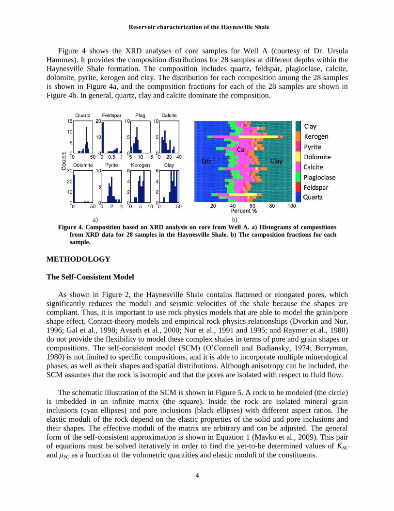
Figure 4 shows the XRD analyses of core samples for Well A (courtesy of Dr. Ursula

Hammes). It provides the composition distributions for 28 samples at different depths within the

Haynesville Shale formation. The composition includes quartz, feldspar, plagioclase, calcite,

dolomite, pyrite, kerogen and clay. The distribution for each composition among the 28 samples

is shown in Figure 4a, and the composition fractions for each of the 28 samples are shown in

Figure 4b. In general, quartz, clay and calcite dominate the composition.

a) b)

Figure 4. Composition based on XRD analysis on core from Well A. a) Histograms of compositions

from XRD data for 28 samples in the Haynesville Shale. b) The composition fractions for each

sample.

METHODOLOGY

The Self-Consistent Model

As shown in Figure 2, the Haynesville Shale contains flattened or elongated pores, which

significantly reduces the moduli and seismic velocities of the shale because the shapes are

compliant. Thus, it is important to use rock physics models that are able to model the grain/pore

shape effect. Contact-theory models and empirical rock-physics relationships (Dvorkin and Nur,

1996; Gal et al., 1998; Avseth et al., 2000; Nur et al., 1991 and 1995; and Raymer et al., 1980)

do not provide the flexibility to model these complex shales in terms of pore and grain shapes or

compositions. The self-consistent model (SCM) (O’Connell and Budiansky, 1974; Berryman,

1980) is not limited to specific compositions, and it is able to incorporate multiple mineralogical

phases, as well as their shapes and spatial distributions. Although anisotropy can be included, the

SCM assumes that the rock is isotropic and that the pores are isolated with respect to fluid flow.

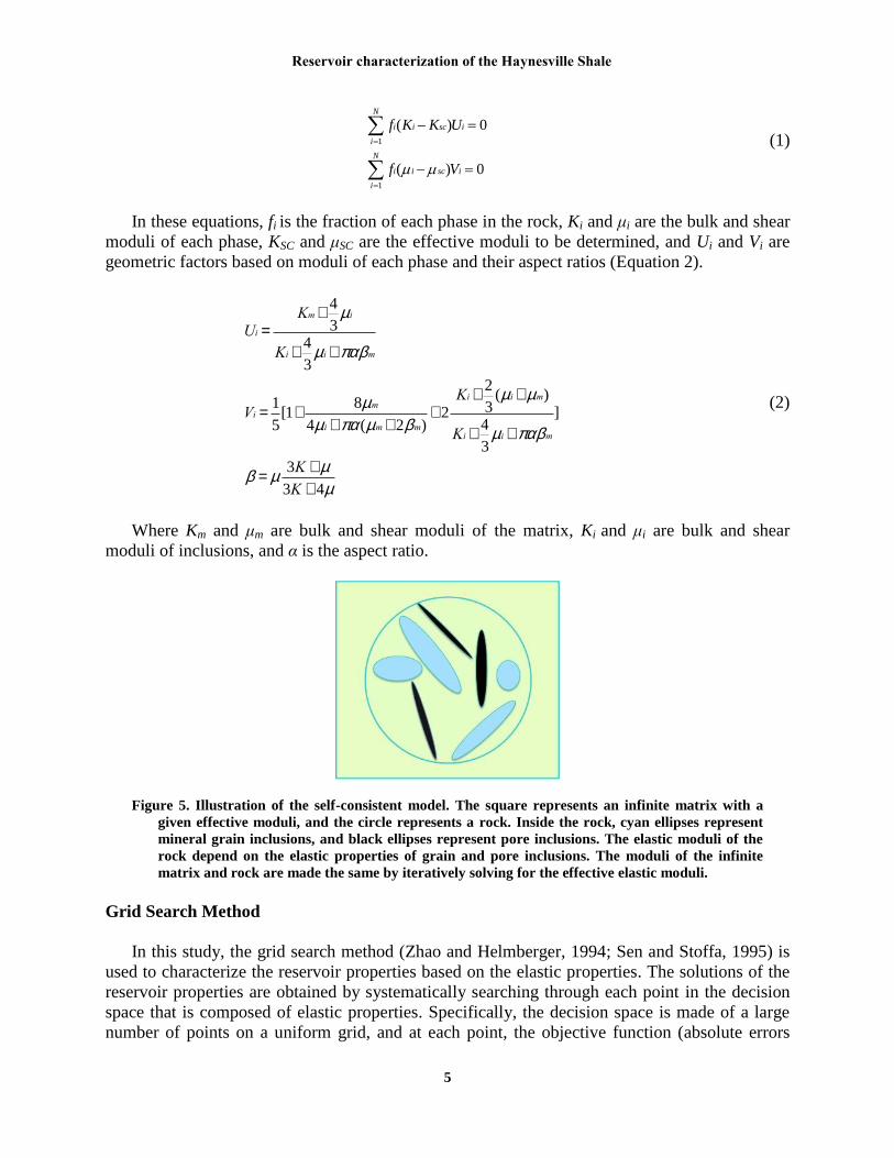
The schematic illustration of the SCM is shown in Figure 5. A rock to be modeled (the circle)

is imbedded in an infinite matrix (the square). Inside the rock are isolated mineral grain

inclusions (cyan ellipses) and pore inclusions (black ellipses) with different aspect ratios. The

elastic moduli of the rock depend on the elastic properties of the solid and pore inclusions and

their shapes. The effective moduli of the matrix are arbitrary and can be adjusted. The general

form of the self-consistent approximation is shown in Equation 1 (Mavko et al., 2009). This pair

of equations must be solved iteratively in order to find the yet-to-be determined values of KSC

and μSC as a function of the volumetric quantities and elastic moduli of the constituents.


5

1

1

( ) 0

( ) 0

N

i i sc i

i

N

i i sc i

i

f K K U

f V

(1)

In these equations, fi is the fraction of each phase in the rock, Ki and μi are the bulk and shear

moduli of each phase, KSC and μSC are the effective moduli to be determined, and Ui and Vi are

geometric factors based on moduli of each phase and their aspect ratios (Equation 2).

Ui =Km+

4

3mi

Ki +4

3mi + pabm

Vi =1

5[1+

8mm

4mi +pa(mm+ 2bm)+ 2

Ki +2

3(mi +mm)

Ki +4

3mi + pabm

]

b = m3K +m

3K + 4m

(2)

Where Km and μm are bulk and shear moduli of the matrix, Ki and μi are bulk and shear

moduli of inclusions, and α is the aspect ratio.

Figure 5. Illustration of the self-consistent model. The square represents an infinite matrix with a

given effective moduli, and the circle represents a rock. Inside the rock, cyan ellipses represent

mineral grain inclusions, and black ellipses represent pore inclusions. The elastic moduli of the

rock depend on the elastic properties of grain and pore inclusions. The moduli of the infinite

matrix and rock are made the same by iteratively solving for the effective elastic moduli.

Grid Search Method

In this study, the grid search method (Zhao and Helmberger, 1994; Sen and Stoffa, 1995) is

used to characterize the reservoir properties based on the elastic properties. The solutions of the

reservoir properties are obtained by systematically searching through each point in the decision

space that is composed of elastic properties. Specifically, the decision space is made of a large

number of points on a uniform grid, and at each point, the objective function (absolute errors


6

between the modeled and observed grid points) is evaluated. The point that provides the

minimum value of the objective function corresponds to the best solution of the reservoir

properties. In this work, we not only obtained the best solution, but also a probability distribution

of multiple solutions. The advantage of the grid search method is that the range of values for the

decision space can be specified and all the possible solutions are equally considered without any

bias. However, the disadvantage of the grid search method is that it can be time consuming and

computationally expensive, depending on the number of points in the decision space. In this

study, 1000 points were used at about 600 depth locations (~ 300 ft sampled at 0.5 ft). When

more reservoir or elastic properties are include, the computational cost increases exponentially.

In addition, the range of values for the decision space should be carefully selected in order to

include all physically reasonable possibilities.

Generally, the P- and S-impedances that form the decision space can be inverted from the

seismic data. In this study we used only well log P-impedance data because the rock physics

modeling was most accurate for P-wave data. S-impedance will be looked at in the near future.

The detailed procedure is shown in Figure 6. From the calibration well (Well A), we calibrated a

SCM with reasonable composition assemblages and pore shapes. Then 1000 porosity values that

were uniformly distributed at each depth were input into the SCM. The resulting P-impedance

values represented the decision space. After that, the observed P-impedances from both Well A

and Well B were compared with the modeled P-impedances, and the absolute errors between

them were calculated as the objective function. By evaluating the objective function, the porosity

was estimated. The modeled P-impedance that provided the smallest absolute error corresponded

to the best solution of porosity, and the ones that provided larger absolute errors corresponded to

solutions with lower probabilities.

Figure 6. Flowchart of the method used in this study. A uniform distribution of porosity was input

into the SCM model, calibrated from Well A to calculate the P-impedance in the decision space.

Then the absolute error between the modeled and observed P-impedance from Well A and B was

calculated. The distribution of porosity was estimated by evaluating the objective function and

selecting multiple solutions.


7

RESULTS

Rock Physics Modeling

The SCM was used to provide the relationship between the reservoir properties and elastic

properties. The reservoir properties include the porosity, pore aspect ratio and composition. In

this study, we focused on the relationships between P-impedance and the porosity, while

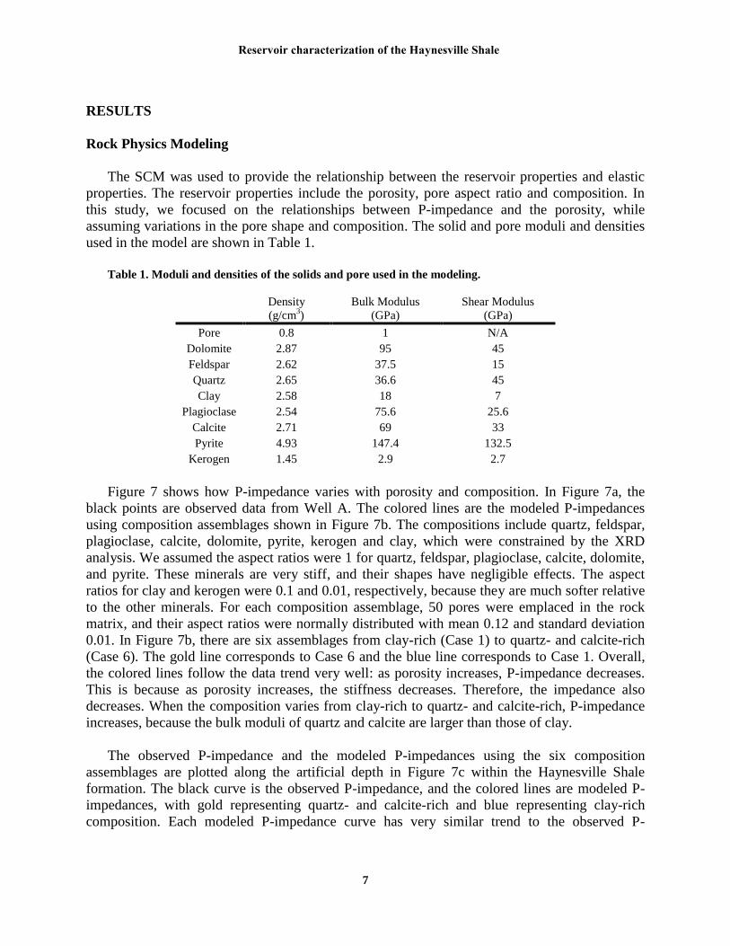
assuming variations in the pore shape and composition. The solid and pore moduli and densities

used in the model are shown in Table 1.

Table 1. Moduli and densities of the solids and pore used in the modeling.

Density

(g/cm3)

Bulk Modulus

(GPa)

Shear Modulus

(GPa)

Pore 0.8 1 N/A

Dolomite 2.87 95 45

Feldspar 2.62 37.5 15

Quartz 2.65 36.6 45

Clay 2.58 18 7

Plagioclase 2.54 75.6 25.6

Calcite 2.71 69 33

Pyrite 4.93 147.4 132.5

Kerogen 1.45 2.9 2.7

Figure 7 shows how P-impedance varies with porosity and composition. In Figure 7a, the

black points are observed data from Well A. The colored lines are the modeled P-impedances

using composition assemblages shown in Figure 7b. The compositions include quartz, feldspar,

plagioclase, calcite, dolomite, pyrite, kerogen and clay, which were constrained by the XRD

analysis. We assumed the aspect ratios were 1 for quartz, feldspar, plagioclase, calcite, dolomite,

and pyrite. These minerals are very stiff, and their shapes have negligible effects. The aspect

ratios for clay and kerogen were 0.1 and 0.01, respectively, because they are much softer relative

to the other minerals. For each composition assemblage, 50 pores were emplaced in the rock

matrix, and their aspect ratios were normally distributed with mean 0.12 and standard deviation

0.01. In Figure 7b, there are six assemblages from clay-rich (Case 1) to quartz- and calcite-rich

(Case 6). The gold line corresponds to Case 6 and the blue line corresponds to Case 1. Overall,

the colored lines follow the data trend very well: as porosity increases, P-impedance decreases.

This is because as porosity increases, the stiffness decreases. Therefore, the impedance also

decreases. When the composition varies from clay-rich to quartz- and calcite-rich, P-impedance

increases, because the bulk moduli of quartz and calcite are larger than those of clay.

The observed P-impedance and the modeled P-impedances using the six composition

assemblages are plotted along the artificial depth in Figure 7c within the Haynesville Shale

formation. The black curve is the observed P-impedance, and the colored lines are modeled P-

impedances, with gold representing quartz- and calcite-rich and blue representing clay-rich

composition. Each modeled P-impedance curve has very similar trend to the observed P-


8

impedance curve. From clay-rich to quartz- and calcite-rich, P-impedance increases. The

crossplot of observed and modeled P-impedances (Figure 7d) also shows their similarity.

a) b)

c) d)

Figure 7. a) Crossplot of P-impedance versus porosity with different composition assemblages for

Well A. Black points are from well log data in the Haynesville Shale formation. Colored lines are

SCM approximations for six different cases, and the numbers on the colored lines are case

numbers, which are consistent with the six composition assemblages shown in b). b) The six cases

with different composition assemblages that consist of quartz, feldspar, plagioclase, calcite,

dolomite, pyrite, kerogen and clay. c) P-impedances from well log data (black curve) and SCM

approximations (colored curves). The colors of the SCM approximations are the same as in a). d)

Crossplot of observed versus modeled P-impedances. Colors are the same as in a) and c). The

black line is a one-to-one line.

The effect of pore shape on P-impedance is shown in Figure 8. Five cases with different

distributions of pore aspect ratios (Figure 8a) were tested. For the five cases, aspect ratios for 50

pores were normally distributed with mean values 0.04, 0.08, 0.15, 0.3, and 0.95, and standard

deviation 0.02. The composition for each case was fixed as 38% quartz, 30% clay, 14%

limestone, 7.8% plagioclase, 5% kerogen, 3% dolomite, 2% pyrite, and 0.2% feldspar. The

aspect ratios were 1 for quartz, feldspar, plagioclase, calcite, dolomite, and pyrite, 0.1 for clay

and 0.01 for kerogen. This composition assemblage is consistent with the modeling result of

composition effect and the average percentage of each composition from the XRD analysis.

4 6 8 10 12 14 16

5550

5600

5650

5700

5750

5800

Art

iric

ial D

ep

th f

t

Ip (km/s)(g/cc)

Well A

Real

5 7 9 11 13 155

7

9

11

13

15

Observed Ip (km/s)(g/cc)

Mo

de

led

Ip

(km

/s)(

g/c

c)

Well A


9

a) b)

c) d)

Figure 8. a) The five different pore aspect ratio distributions. Each of them contains 50 pores, with

mean value 0.04, 0.08, 0.15, 0.3, and 0.95, respectively, and standard deviation of 0.02. b)

Crossplot of P-impedance versus porosity with different pore aspect ratio distributions for Well

A. Black points are from well log data in the Haynesville Shale formation. Colored lines are SCM

approximations for different pore aspect ratio distributions based on a). The colors of the pore

aspect ratio distributions are the same as in a). c) P-impedances from well log data (black curve)

and SCM approximations using the pore aspect ratio distributions based on a). The colors of the

SCM approximations are the same as in a). d) Crossplot of observed versus modeled P-

impedances. Colors are the same as in a) b) and c). The black line is a one-to-one line.

In Figure 8b, the black points are observed data from Well A. The colored lines are the

modeled P-impedances using the distributions of pore aspect ratio as Figure 8a shows. The

magenta line corresponds with the pore aspect ratios that have the largest mean value, and the

blue line corresponds to the pore aspect ratios that have the smallest mean value. The lines with

larger mean values of pore aspect ratios have higher P-impedance because larger pore aspect

ratios have greater stiffness. Within each line, P-impedance decreases as porosity increases,

which is consistent with the trend from the data. Variable pore shape, in addition to

compositional variation, provides at least a partial explanation for the scatter in the data. The

observed P-impedance and the modeled P-impedances using the five pore aspect ratio

distributions are plotted along the artificial depth in Figure 8c within the Haynesville Shale

formation. The black curve is the observed P-impedance, and the colored lines are modeled P-

impedances. Each modeled P-impedance curve has very similar trend to the observed P-

impedance curve. The results show that for Well A, the pore aspect ratio in the Haynesville Shale

is mainly between 0.08 (green) and 0.15 (red), which is generally consistent with the aspect

0 0.1 0.2 0.3 0.4 0.5 0.6 0.7 0.8 0.9 10

5

10

15

Aspect Ratio

Fre

qu

en

cy

0 0.05 0.1 0.15 0.2 0.256

7

8

9

10

11

12SCM: Well A

fDen

Ip (

km

/s)(

g/c

c)

4 6 8 10 12

5550

5600

5650

5700

5750

5800

Art

iric

ial D

ep

th f

t

Ip (km/s)(g/cc)

Well A

Real

4 6 8 10 124

6

8

10

12

Observed Ip (km/s)(g/cc)

Mo

de

led

Ip

(km

/s)(

g/c

c)

Well A


10

ratios approximation from Figure 2b. The crossplot of observed and modeled P-impedances

(Figure 8d) also shows the similarity among the trends.

Uncertainty Analysis in the Forward Problem

Analysis of the effects of composition (Figure 7) and pore shape (Figure 8) provided inputs

to the SCM. The input parameters for composition were 38% quartz, 30% clay, 14% limestone,

7.8% plagioclase, 5% kerogen, 3% dolomite, 2% pyrite, and 0.2% feldspar; the input pore aspect

ratios were normally distributed with mean value 0.12 and standard deviation 0.01. The SCM

approximation for P-impedance from these parameters is shown in Figure 9. In the crossplot of

P-impedance and porosity (Figure 9a), the P-impedance approximation (blue line) follows the

trend of the data (black points) very well. In Figure 9b, the P-impedance approximation (blue

curve) generally matches with the observed P-impedance in terms of both variation trend and

amplitude. The difference between the observed and modeled P-impedances is mostly around

zero (Figure 9c), with an average of about 5%.

a) b)

c)

Figure 9. a) Crossplot of P-impedance versus porosity for Well A. Black points are from well log

data. The blue line is the SCM approximation with pore aspect ratio ~ N(0.12, 0.012), and

composition assemblage of 38% quartz, 30% clay, 14% limestone, 7.8% plagioclase, 5%

kerogen, 3% dolomite, 2% pyrite, and 0.2% feldspar. b) P-impedances from well log data (black

curve) and the SCM approximation (blue curve) versus artificial depth. c) The difference

between the observed and modeled P-impedances.

The SCM that is calibrated from Well A provides P-impedance when a single porosity curve

is input. Consequently, the uncertainty in the modeled P-impedance will be reflected by the error

0 0.05 0.1 0.15 0.2 0.256

7

8

9

10

11

12SCM: Well A

fDen

Ip (

km

/s)(

g/c

c)

6 7 8 9 10 11 12

5550

5600

5650

5700

5750

5800

Art

iric

ial D

ep

th f

t

Ip (km/s)(g/cc)

Well A

Real


11

in the porosity and vice versa (Figure 10). To assess the uncertainty of porosity and P-impedance

for the whole Haynesville Shale formation, we assumed 500 porosity values that were normally

distributed with mean 0.13 and standard deviation 0.02 (Figure 10a). These mean and standard

deviation values were determined from the observed porosities within the Haynesville Shale

formation, and the number of porosity values (500) makes the distribution smooth and the

computational cost low. When these porosities were input into the SCM, the corresponding P-

impedances were also normally distributed (Figure 10b). To analyze the modeling uncertainty

for each depth within the Haynesville Shale, we assumed 500 porosity values input at each depth

which were normally distributed with mean value the same as the observed porosity, and

standard deviation 0.02 (Figure 10c). Correspondingly, the modeled P-impedances at each depth

were also normally distributed, where the mean values generally matched the observed P-

impedance (Figure 10d). The analysis performed here provided an estimate of the uncertainty in

the forward problem.

a) b)

c) d)

Figure 10. a) Distribution of porosity within the Haynesville Shale formation. Five hundred porosity

values were normally distributed with mean value 0.13 and standard deviation 0.02. b) The

corresponding P-impedances from SCM by using the porosity distribution from a). c) Porosity

input for Well A. The black curve is the observed porosity. At each depth, 500 porosities were set

to be normally distributed with mean value the same as the observed porosity and standard

deviation 0.02. d) Probability of modeled P-impedance from SCM. The black curve is the

observed P-impedance.

0.05 0.1 0.15 0.2 0.250

10

20

30

40

50Porosity distributions

Porosity

Co

un

t

6 7 8 9 100

10

20

30

40

50Ip distributions

Ip (km/s)(g/cc)

Co

un

t


12

Inversion Results from the Grid Search Method

To perform the grid search, 1000 porosity values at about 600 depth locations (~ 300 ft

sampled at 0.5 ft) were uniformly distributed between 0 and 0.25. This number (1000) of

porosity values at each depth is enough to keep accuracy high but computational cost low. The

upper limit (0.25) was selected as about 25% larger than the maximum observed value. Values

above 0.25 were assumed unlikely to occur. The P-impedance was then calculated from the SCM

at every point in the grid. The absolute error between this modeled P-impedance and the one

from Well A (Figure 11a) was calculated as the objective function. At each depth, the modeled

P-impedance with the smallest error corresponds to the best solution of porosity. The P-

impedances with larger errors correspond to porosity solutions with smaller possibility (Figure

11b). Although a grid search method can be time consuming in some cases, here the whole

process only takes about 20 seconds, because the number of grid is not too large. In Figure 11b,

the color is the error in the porosity estimation from the grid search, the green curve is the best

solution of porosity, and the black curve is the observed porosity. The estimated porosity fits the

observed porosity in terms of both variation trend and amplitudes, which indicates that the SCM

and grid search method worked effectively for Well A. The average difference between the

observed and estimated porosities for Well A is about 10%.

a) b)

Figure 11. Grid searching result for Well A (calibration well). a) Observed P-impedance. b) Porosity

estimation. Hot colors represent porosity with smaller error, and cold colors represent porosity

with larger error. The solid black curve is the observed porosity, and the green curve is the

estimated porosity with smallest error.

The same grid search procedure was then performed on the test well (Well B). The

corresponding porosity estimation is shown in Figure 12. The estimated porosity generally

matches the observed porosity for the artificial depth range from 5525 to 5575 ft. Outside this

depth range, although the estimated porosity has larger absolute values than the observed

porosity, the variation trend matches the observed porosity. The average difference between the

observed and estimated porosities for Well B is about 26%.

6 7 8 9 10 11 12

5550

5600

5650

5700

5750

5800

Art

iric

ial D

ep

th f

t

Ip (km/s)(g/cc)

Well A

Real


13

a) b)

Figure 12. Grid searching result for Well B (test well). a) Observed P-impedance. b) Porosity

estimation. Hot colors represent porosity with smaller error, and cold colors represent porosity

with larger error. The black curve is the observed porosity, and the green curve is the estimated

porosity with smallest error.

a) b)

c)

Figure 13. a) Crossplot of P-impedance versus porosity for Well B. Black points are from well log

data. The blue line is the SCM approximation with pore aspect ratio ~ N(0.12, 0.012), and

composition assemblage of 38% quartz, 30% clay, 14% limestone, 7.8% plagioclase, 5%

kerogen, 3% dolomite, 2% pyrite, and 0.2% feldspar. b) P-impedances from well log data (black

curve) and the SCM approximation (blue curve). c) The difference between the observed and

modeled P-impedances.

7 8 9 10 11

5450

5500

5550

5600

5650

5700

Art

iric

ial D

ep

th f

t

Ip (km/s)(g/cc)

Well B

0 0.05 0.1 0.15 0.27

7.5

8

8.5

9

9.5

10

10.5

11SCM: Well B

fDen

Ip (

km

/s)(

g/c

c)

7 8 9 10 11 12

5450

5500

5550

5600

5650

5700

Art

iric

ial D

ep

th f

t

Ip (km/s)(g/cc)

Well B

Real


14

The crossplot of P-impedance versus porosity is very scattered (the correlation coefficient

between them is -0.39) for Well B, and the SCM from Well A does not represent the data points

very well (Figure 13a). Generally, the SCM approximation of P-impedance overestimates the

observed P-impedance (Figure 13b). The difference between the observed and modeled P-

impedance (Figure 13c) is dominated by negative values, which also indicates that the SCM

calibrated from Well A overestimated P-impedance for Well B. As a result, the estimated

porosities (Figure 12b) have larger values than the observed porosity.

DISCUSSION

In this study, the pore shape and composition were first calibrated using the SCM from Well

A. Average parameters from this calibration were then used in the grid search for both Well A

and Well B. Uncertainty exists in the porosity estimation, especially for Well B, because the pore

size, pore shape, and composition may vary spatially within the Haynesville Shale formation. In

addition, the effects of these parameters on seismic velocity may vary from well to well, and

even within the same well. It was found that for Well B, the dominating effect on velocity is pore

shape for the high density and low velocity area, but porosity for the low density and low

velocity area (Spikes and Jiang, 2012). Also, there is non-uniqueness in generating elastic

properties from rock physics models: different combinations of reservoir properties may result in

the same elastic properties and vice versa. In the future, the pore shape and composition will be

considered as variables similar to porosity, and the decision space will include both P- and S-

impedances, in which case the calculation will be exponentially more expensive.

The procedure in this study includes only well log P-impedance data. When seismic data is

also included, the 3D distributions of P- and S-impedances can be obtained. Therefore, it will be

possible to obtain 3D distributions of the reservoir properties. When the seismic data is included,

additional sources of uncertainty will have to be addressed, which includes the noise in the data,

natural variability, and the inversion process. On the one hand, there is non-uniqueness in

seismic inversion, which indicates that different inverted impedances provide equally well-fitted

seismic traces. On the other hand, there is an upscaling issue when comparing P- and S-

impedances from rock physics models with the inverted P- and S-impedances from seismic

inversion. This occurs because impedances from well log data have higher resolution than the

ones from seismic data. The Backus average (Backus, 1962) will be used to solve this upscaling

issue. The Backus average is the long wavelength effective medium approximation. It converts

the measurements at the well log scale to seismic scale by using moving averages with different

window lengths, where the window lengths are based on the frequency of the seismic data.

CONCLUSIONS

This study provides a method that combines the rock physics modeling with a grid search

method to characterize the reservoir property for the Haynesville Shale using well log data. The

self-consistent model that considers composition and pore shape effects works well for the

calibration well. It provides the relationship between the porosity and P-impedance with

constraints on the composition and pore shape for the Haynesville Shale. Combining this self-

consistent model with a grid search method provides 1D distributions of porosity at the well

locations. The porosity estimation for the calibration well matches with the observed porosity in


15

terms of both variation trend and absolute value; and the porosity estimation for the test well

matches the variation trend with the observed porosity. When combined with seismic data from

3D volumes, we can obtain 3D distributions of P- and S-impedances, and therefore characterize

3D distributions of the reservoir properties. In addition, although various gas shales may be

different in terms of the properties that most significantly affect the seismic velocities, the

procedures developed for the Haynesville Shale could be applied to other gas shales to

characterize their reservoir properties.

ACKNOWLEDGEMENTS

We thank BP for providing the data. The Exploration and Development Geophysics

Education and Research (EDGER) Forum at the University of Texas at Austin and the American

Chemical Society Grant PRF# 51157-DNI8 supported this work.

REFERENCES

Avseth, P., Dvorkin, J., Mavko, G., and J. Rykkje, 2000, Rock physics diagnostic of North Sea sands: Link between

microstructure and seismic properties: Geophysical Research Letters, 27, 2761–2764.

Bachrach, R., 2006, Joint estimation of porosity and saturation using stochastic rock-physics modeling: Geophysics,

71, o53–o63.

Backus, G., 1962, Long-wave elastic anisotropy produced by horizontal layering, Journal of Geophysical Research,

67, 4427–4440

Berryman, J., 1980, Long-wavelength propagation in composite elastic media I. Spherical inclusions: Journal of the

Acoustical Society of America, 68, 1809–1819.

Curtis, M.E., Ambrose, R.J., Sondergeld, C.H., and C.S. Rai, 2010, Structural characterization of gas shales on the

micro- and nano-scales: Canadian Society for Unconventional Gas/Society of Petroleum Engineers, doi:

10.2118/137693-MS.

Dvorkin J. and A. Nu, 1996, Elasticity of high-porosity sandstones: theory for two North Sea data sets: Geophysics,

61, 1363–1370.

Eidsvik, J., Avseth, P., More, H., Mukerji, T., and G. Mavko, 2004, Stochastic reservoir characterization using

prestack seismic data: Geophysics, 69, 978–993.

Gal D., Dvorkin J., and A. Nur, 1998, A physical model for porosity reduction in sandstones: Geophysics, 63, 454–

459.

Grana, D. and E. Della Rossa, 2010, Probabilistic reservoir-properties estimation integrating statistical rock physics

with seismic inversion: Geophysics, 75, o21–o37.

Hammes, U., Eastwood. R., Rowe, H. D., and R. M. Reed, 2009, Addressing conventional parameters in

unconventional shale-gas systems: depositional environment, petrography, geochemistry, and petrophysics of

the Haynesville shale, in Carr, T., T. D’Agostino W. A. Ambrose, J. Pashin, and N. C. Rosen, eds.,

Unconventional energy resources: making the unconventional conventional: 29th Annual GCSSEPM

Foundation Bob F. Perkins Research Conference, Houston, p. 181–202.

Hammes, U., Hamlin, H. S., and E. E. Thomas, 2011, Geologic analysis of the Upper Jurassic Haynesville Shale in

east Texas and west Louisiana: American Association of Petroleum Geologists Bulletin, 95, 1643–1666.

Mavko, G., Mukerji, T., and J. Dvorkin, 2009, The rock physics handbook: Cambridge University Press.

Mukerji, T., Jorstad, A., Avseth, P., Mavko, G., and J. R. Granli, 2001, Mapping lithofacies and pore-fluid

probabilities in a North Sea reservoir: seismic inversions and statistical rock physics: Geophysics, 66, 988-1001.

Nur, A., Marion, D., and H. Yin, 1991. Wave velocities in sediments. In Shear Waves in Marine Sediments, ed. J.M.

Hovem, M.D. Richardson, and R.D. Stoll. Dordrecht: Kluwer Academic Publishers, pp. 131–140.

Nur, A., Mavko, G., Dvorkin, J., and D. Gal, 1995. Critical porosity: the key to relating physical properties to

porosity in rocks. In Proceedings of the 65th Annual International Meeting, 878. Tulsa, OK: Society of

Exploration Geophysicists.

O’Connell, R. and B. Budiansky, 1974, Seismic velocities in dry and saturated crack solids: Journal of Geophyscis

Research, 79, 5412–5426.


16

Raymer, L.L., Hunt, E.R., and J.S. Gardner, 1980. An improved sonic transit time-to-porosity transform.

Transactions of the Society of Professional Well Log Analysts, 21st Annual Logging Symposium, Paper P.

Sen, M. and P.L. Stoffa, 1995, Global optimization methods in geophysical inversion: ELSEVIER Science

Spikes, K.T., Mukerji,T., Dvorkin, J., and G. Mavko, 2007, Probabilistic seismic inversion based on rock-physics

models, Geophysics, 72, R87–R97.

Spikes, K.T., and M. Jiang, 2012, Rock physics relationships between elastic and reservoir properties in the

Haynesville Shale, American Association of Petroleum Geologists Memoir, in revision.

Wang, F. P. and U. Hammes, 2010, Effects of reservoir factors on Haynesville fluid flow and production: World Oil,

231, D3–D6.

Zhao, L.-S. and D.V. Helmberger, 1994, Source estimation from broadband regional seismograms: Bulletin of

Seismological Society of America, 84, 91–104.

CHARACTERIZING RESERVOIR PROPERTIES OF THE … · characterizing reservoir properties of the...

Documents

Transcript of CHARACTERIZING RESERVOIR PROPERTIES OF THE … · characterizing reservoir properties of the...