Characterization of Fibre Suspension Flows at Papermaking Consistencies

Amir Raghem Moayed

A thesis submitted in conformity with the requirements for the de ree of Doctor of Philosophy

Graduate Department of 8 hemical En 'neering and Applied Chemistry University of ? oronto

@ Copyright by Amir Raghem Moayed 1999

National Library 1*1 of Canada Bibliothhue nationale du Canada

Acquisitions and Acquisitions et Bibliographic Services sendces bibliographiques 395 Wellington Street 395. rue Wellington Ottawa ON K1 A ON4 OttawaON KlAON4 Canada Canada

The author has granted a non- exclusive licence allowing the National Library of Canada to reproduce, loan, distribute or sell copies of this thesis in microform, paper or electronic formats.

The author retains ownership of the copyright in this thesis. Neither the thesis nor substantial extracts from it may be printed or otherwise reproduced without the author's permission.

L'auteur a accorde une licence non exclusive permettant a la Bibliotheque nationale du Canada de reproduire, preter, distribuer ou vendre des copies de cette these sous la fome de microfiche/film, de reproduction sur papier ou sur format electronique .

L'auteur consewe la propriete du droit d'auteur qui protege cette thltse. Ni la these ni des extraits substantiels de celle-ci ne doivent &re imprimes ou autrement reproduits sans son autori sation.

Characterization of Fibre Suspension Flows at Papermaking Consistencies

Degree and year of convocation: Ph.D. (1999) Graduate Department of Chemical Engineering and Applied Chemistry

Amir Raghem Moayed

University of Toronto

Abstract

Accurate and effective quality control of the manufacture of information grade paper is

becoming the primary papermaking concern with the recent and upcoming advances in

modern printing technology. An important quality issue, but poorly understood phe-

nomenon, is the interactions between papermaking flow characteristics and the unifor-

mity of fibrous suspensions. To extend knowledge and understanding of these complex

interactions, the behavior of a flowing pulp suspension in a grid generated turbulence flow

field was experimentally studied and the scale dependency of the suspension uniformity

was modeled. A Dynamic Panoramic View technique was developed simultaneously to

measure and quantify the suspension local mass variability along the stream-wise direc-

tion as well as the transverse direction. The effects of mean flow velocity, concentration,

and local flow characteristics on the local mass variability of a representative hardwood

kraft pulp were studied. A model was developed to characterize the rate of fibre ag-

gregation in a decaying turbulent Aow field. This model was found to be in excellent

agreement with experimental data.

The experimental set-up and methodology were designed in such a fashion that the

whole system, in general, and the present experimental result, in particular, provide

useful tools for Computational Fluid Dynamics modeling purposes.

A statistical geometric model was developed to characterize internal structure of fibre

flocs and aggregate size distributions. The quality of a pulp suspension flow was char-

acterized by model parameters, and turbulence energy requirements can be drawn from

the model. The model equations were found in excellent agreement with experimental

data.

iii

Acknowledgements

I wish to express my gratitude to my supervisors, Professor D.C.S Kuhn and Professor

C.T.J. Dodson, for their assistance, guidance and time provided on a continual basis.

I am grateful to my Reading 'Committee for their advice and clarifying remarks.

Cheerful thanks are due to Professors M.T. Kortschot and D.E. Cormack for their con-

structive criticisms and Professor David Goring for sharing with me his wisdom.

I would like to extend my appreciation to Electronic and Machine Shops for their

assistance during the development of the experimental apparatus. Many thanks go to

Mr. Dan Tomchyshyn for his computer support.

I wish to thank my family for their sincere encouragement and emotional supports.

Contents

1 Introduction 1

Literature Review 7

. . . . . . . . . . . . . . . . . . . . . . . . 2.1 Pulp Flow Characteristics 8

. . . . . . . . . . . . . . . . . . . . . . 2.1.1 Fully Developed Flows 8

. . . . . . . . . . . . . . . . . . . . . . . . . 2.1.2 Developing Flows 8

. . . . . . . . . . . . 2.2 Characteristics of Decaying Turbulent Flows 10

. . . . . . . . . . . . . . . . . . . . . 2.2.1 Decay of Kinetic Energy 10

. . . . . . . . . . . . . . . . . 2.2.2 Dissipation of Kinetic Energy 11

. . . . . . . . . . . . . . . . . . . . . . . 2.3 Characterizing Flocculation 12

. . . . . . . . . . . . . . . 2.3.1 Turbulence Flocculation Statistics 12

2.3.2 Flocculation Geornetrics and Statistical Geornetrics . . . . 16

. . . . . . . . . . . . . . . . . . . . . . . . . 2.4 Measurement Techniques 18

. . . . . . . . . . . . . . . . . . . . . . . . 2.4.1 Flow Measurements 18

. . . . . . . . . . . . . . . . . . . 2.4.2 Flocculation Measurements 19

. . . . . . . . . . . . . . . . . . . . . . . 2.5 Modeling Fibre Flocculation 23

3 Experimental Design and Methodology 25

. . . . . . . . . . . . . . . . . . . . . . . . . . . . . . 3.1 Flow loop system 26

. . . . . . . . 3.2 Elements of the Dynamic Panoramic View System 29

. . . . . . . . . . . . . . . . . . . . . . . . . 3.2.1 Video Micrometer 32

. . . . . . . . . . . . . . . . . 3.3 Imaging performance and calibration 35

. . . . . . . . . . . . . . . . . . . . 3.3.1 CCD Camera performance 35

. . . . . . . . . . . . . . . . . . . . . . . . . . . . . 3.3.2 Calibration 38

. . . . . . . . . . . . . . . . . . . . . . . 3.4 Flocculation Measurements 40

. . . . . . . . . . . . . . . . . . . . . . . . . 3.4.1 Number of Images 41

. . . . . . . . . . . . . . . . . . . . . . . . . . . 3.4.2 Image Analysis 42

. . . . . . . . . . . . . . . . . . . . . . . . . . . . . . . . . . . . 3.5 Closure 44

4 Characterization of Fibre Flocculation in Turbulent Decaying Flows

. . . . . . . . . . . . . . . . . . . . . . . . . . . . . . . . . 4.1 Introduction

. . . . . . . . . . . . . . . . . . . . . . . . . . . . . . . . 4.2 Experimental

. . . . . . . . . . . . . . . . . . . . . . . . . . . . . . . 4.2.1 Material

4.2.2 Experimental procedure and techniques . . . . . . . . . . .

. . . . . . . . . . . . . . . . . . . . . . . . . . 4.3 Results and Discussion

4.3.1 Flow Field Analysis . . . . . . . . . . . . . . . . . . . . . . . .

. . . . . . . . . . . . . . 4.3.2 Longitudinal Flocculation Intensity

. . . . . . . . . . . . . . . . . . 4.3.3 Flocculation intensity profiles

. . . . . . . . . . . . . . . . . . . . . . . . . . . . 4.3.4 Homogeneity

. . . . . . . . . . . . . . . . . . . . . . . 4.3.5 Effect of flow velocity

. . . . . . . . . . . . . . . . . . . . . . . . 4.3.6 Effect of consistency

. . . . . . . . . . . . . . . . . . . 4.3.7 Characterizing flocculation 68

4.4 Closure . . . . . . . . . . . . . . . . . . . . . . . . . . . . . . . . . . . . 74

5 Characteristics of Fibre Flocs in Turbulent Flows 77

5.1 Introduction . . . . . . . . . . . . . . . . . . . . . . . . . . . . . . . . . 77

5.2 Transverse floc size distributions . . . . . . . . . . . . . . . . . . . . 79

5.2.1 Stochastic Fibre Clumps . . . . . . . . . . . . . . . . . . . . . 81

. . . . . . . . . . . . . . . . . . . . . . . . . . . . . . 5.2.2 Variability 84

5.2.3 Floc size estimates from fluid permeation . . . . . . . . . . 88

5.2.4 Comparison with the relative turbulent diffusion theory . 93

5.3 Longitudinal floc size distributions . . . . . . . . . . . . . . . . . . . 95

5.3.1 Suspension Quality Analysis . . . . . . . . . . . . . . . . . . . 99

5.3.2 Comparison with experimental data . . . . . . . . . . . . . . 100

. . . . . . . . . . . . . . . . . . . . . . . . . . . . . . . . . . . . 5.4 Closure 101

6 Conclusions 106

6.1 Flow/Mass Variability Analysis . . . . . . . . . . . . . . . . . . . . . 106

6.2 Flow/Floc Scale Analysis . . . . . . . . . . . . . . . . . . . . . . . . . 108

6.3 Implementation . . . . . . . . . . . . . . . . . . . . . . . . . . . . . . . 109

6.4 Recommendations . . . . . . . . . . . . . . . . . . . . . . . . . . . . . 110

Appendix A

References

vii

List of Figures

A schematic dzagrarn of a papermaking headbox. . . . . . . . . . . . . . A jet issuing from the slice of a headbox (courtesy of D. Mondor,

wwwB.sympatico.ca/denis. mondor). . . . . . . . . . . . . . . . . . . . . Forming section control of a forming paper near the slice of a headbox

(after Dentec Measurement Technology). . . . . . . . . . . . . . . . . . .

Suspension flow regimes in pipe flow. . . . . . . . . . . . . . . . . . . . . The principle offEocculation measurement using ampact probes (afler Nere-

lius et al. 1972). . . . . . . . . . . . . . . . . . . . . . . . . . . . . . . . Monitoring ftoc size distributions using a light transmission technique. .

Flow loop system used for measuring fEocculation in a turbulent decaying

flow. . . . . . . . . . . . . . . . . . . . . . . . . . . . . . . . . . . . . .

Geometry of the flow cell used for generating turbulent decaying flow field.

Flow distributors and corresponding flow patterns produced by them . . . A schematic diagram of the imaging sglstem facilities and set-up used for

flocculation measurements. . . . . . . . . . . . . . . . . . . . . . . . . .

Top view of nine identical cylinders with an angular viewing error (top)

and with a telecentric view (bottom). . . . . . . . . . . . . . . . . . . . . A measurement area transposed by the reference window. . . . . . . . . . Test section of the turbulence rig and measurement area used for floccu-

lation measurements. . . . . . . . . . . . . . . . . . . . . . . . . . . . . . Images of the background (bottom), Mylarfilm before (top) and after (mid-

dle) the background cancellation operation. . . . . . . . . . . . . . . . . Scans through the images of the background (bottom) and Mylar film before

(top) and after (middle) the background cancellation operation . . . . . . The relationship between mean gray value and transmitted light intensity

passed through layers of the Mylar film. . . . . . . . . . . . . . . . . . . Calibration curve for a hardwood semi-bleached fibre suspension. . . . . . Flow chart of image analysis. . . . . . . . . . . . . . . . . . . . . . . . . An egective image area from cutting image operation. . . . . . . . . . .

A schematic diagram of a headbox with the rectifier roller turbulence gen-

erator. . . . . . . . . . . . . . . . . . . . . . . . . . . . . . . . . . . . . A schematic diagram of a test headbox (top) and diferent types of turbu-

lence generators (bottom) investigated by Ilmonnzemi et. al. (1 986). . . Schematic diagram of the grid configuration and measuring area in the

turbulence r ig test section, 50 cm downstream of the rig's inlet. . . . . . Schematic diagram of the flow field near the grids. . . . . . . . . . . . . Longitudinal fEocculatzon intensity at Ub = 0.45mlsec and C, = 0.54% . Longitudinal flocculation intensity at Ub = 0.45rnlsec and C,,, = 0.5% . .

4.7 Longitudinal jlocculation intensity at Ub = 0.26mlsec and C, = 0.54% .

4.8 Longitudinal flocculation intensity at Ub = 0.26mlsec and C,,, = 0.42% .

4.9 Longitudinal flocculation intensity at Ub = 0.45mlsec and C, = 0.42% .

4.10 Longitudznal fEocculation intensity at Ub = 0.26mlsec and C, = 0.5% . .

4.11 Flocculation intensity profiles at Ub = 0.45mlsec and C,,, = 0.54% . . . . 4.12 Flocculation intensity profiles at Ub = 0.26mlsec and Cm = 0.54% . . . . 4.13 Flocculation intensity profiles at Ub = 0.45mlsec and Cm = 0.5% . . . .

4.14 Flocculation intensity profiles at Ub = 0.26mlsec and C, = 0.5% . . . . 4.15 Flocculation intensity profiles at Ub = 0.45mlsec and Cm = 0.37% . . . . 4.16 Schematic diagram of the flow pattern near the exit of two grids. . . . . . 4.17 Homogeneity i n the fEocculation intensity behind the grids and across the

width of the channel (y = f d). . . . . . . . . . . . . . . . . . . . . . . . . 4.18 Effect of bulk flow velocity on the j2occulation intensity at C, = 0.42%. .

4.19 Effect of pulp consistency on the fEocculation intensity at Ub = 0.45mlsec

4.20 Comparison between the measured turbulence intensity and power law

model of the decay of turbulence (data from d'lncau (1983)). . . . . . . 4.21 Variation of j?occulation intensity with bulk velocity at different consis-

tencies at x/d = 27. . . . . . . . . . . . . . . . . . . . . . . . . . . . . . 4.22 The correlation between fEocculation intensity and Reynolds number and

mean consistency with r2 = 0.96 at x/d = 27. . . . . . . . . . . . . . . . 4.23 Comparison between the empirical power law and fEocculation intensity

downstream of the grid at Ub = 0.45m/s. . . . . . . . . . . . . . . . . .

4.24 The Self-preservation curve of the ftocculation intensity downstream of a

. . . . . . . . . . . . . . . . . . . . grid generated tu~bulence ( x / d > 9).

a) (lefl) Variation of the error associated with approximation (5.6) and

b) (right) with that of approximation (5.7) relative to the true value (5.4).

The shape of the self-similarity distribution function (5.7) shifis from a

negative exponential function t o a log-normal type as the intrinsic jloccu- - . . . . . . . . . . . . . . . . . . . . . . . . lation parameter, k, increases.

T h e relationship between the dimensionless standard deviation a, and the

mean 3 of jloc size, o n a log-log plot. The dot points are calculated from

equations (5.9) and (5.10) and the solid line i s the best linear regression

fit t o these points, which has a slope of 0.67. . . . . . . . . . . . . . . . .

E ' e c t of sheet density o n pore size distribution. Broken line i s the log-

linear plot of the experimental data (Corte and Lloyd, 1965) for softwood

(leff) and hardwood (right) sulfate pulp. Solid line represents the model

equation (6) in (Dodson and Sampson, 1996). . . . . . . . . . . . . . . .

The relationship between the mean and the standard deviation of floc sizes,

calculated from equations (5-14) and (5-15). Parameters of these equa-

tions are estimated from the pore size distribution data (Corte and Lloyd

1965) for the softwood ( [e f t ) and hardwood (Irght) sulphate pulp. T h e solid

line is the regression equation obtained from a VBR technique (Farnood

1996). . . . . . . . . . . . . . . . . . . . . . . . . . . . . . . . . . . . . .

The relationship between the calculated mean jloc size (equation (5.14))

. . . . . . . . . . . . . . . . . . . . . . . . and measured mean pore size.

5.7 Effect of sheet density on mean floc size. . . . . . . . . . . . . . . . . . . 94

5.8 E$ect of flocculation on the floc size distributions calculated from mea-

sured pore size distributions. . . . . . . . . . . . . . . . . . . . . . . . . . 95

5.9 Effect of sheet density on floc size distributions calculated from the mea-

sured pore size. . . . . . . . . . . . . . . . . . . . . . . . . . . . . . + . . 96

5.10 A schematic diagram of the proposed longitudinal ftocculation model. Floc-

culation i s defined as the successive movements of the contact points along

the flour direction. . . . . . . . . . . . . . . . . . . . . . . . . . . . . . . . 97

5.11 E$ect of the number of fibre perflocs on floc size distribution. . . . . . . 99

5.12 Effect of the parameter k on floc size distribution. . . . . . . . . . . . . 100

5.13 Comparison between the theoretical ftoc size distribution and experimental

data for hardwood fibres at consistency 1.35%. . . . . . . . . . . . . . . 103 5.14 Comparison between the theoretical jloc size distribution and experimental

data for hardwood fibres at consistency 0.5%. . . . . . . . . . . . . . . . 104 5.15 Comparison between the theoretical j2oc size distribution and experimental

data for softwood fibres at consistency 0.5%. . . . . . . . . . . . . . . . . 104 5.16 Comparison between the theoretical floc size distribution and experimental

data for softwood fibres at consistency 1.35%. . . . . . . . . . . . . . . . 105 5.17 Comparison between the present model and Hourani's model for hardwood

fibres at consistency 0.5%. . . . . . . . . . . . . . . . . . . . . . . . . . . 105

xii

List of Tables

. . . . . . . . . . . . . . . . . . . . . . . 3.1 Parameters of the Image Grabber 35

. . . . . . . . . . . . . . . . . . . . 4.1 Pulp characteristics (four replicates) 51

. . . . . . . . . . . . . . . . . . . . . . . . . . . . 4.2 Experimental variables 53

5.1 Parameters of the pore and apparent floc size distributions- Effect of

. . . . . . . . . . . . . . . . . . . . . . . . . . . . . . . . . . flocculation 90

5.2 Parameters of the pore and apparent floc size distributions- Effect of sheet

. . . . . . . . . . . . . . . . . . . . . . . . . . . . . . . . . . . . . density 91

5.3 Estimated parameters of the theoretical longitudinal/Eulerian floc size

distribution from Hourani's experiments . . . . . . . . . . . . . . . . . . . 102

xiii

Nomenclature

fibre aspect ratio

mean concentration

coefficient of variation in concentration

turbulent concentration

mass pulp consistency

volumetric concentration

size of a pixel in a CCD sensor

depth of field

power spectrum

frequency

longitudinal autocorrelation coefficient for flow

longitudinal autocorrelation coefficient for concentration

ratio of the focal length to the diameter of the entrance iris

22 flocculation intensity, m

free-fibre length, eddy size

image gray level value

transverse autocorrelation coefficient for flow

transverse autocorrelation coefficient for concentration

couple-particle diffusivity

xiv

floc interaction parameter, suspension uniformity parameter

macro floc length scale in stream-wise direction

doppler wave length

image magnification

average number of fibre crossings along a scan line per floc

average number of fibre crossings in a plane per floc

fibre crowding factor

mean number of signal crossings with per unit time

number of fibre contacts per fibre

number of particle per unit volume

self-similar transverse floc size distribution

Reynolds number

probability that two particles inside of a floc are separated by a distance r at time t

turbulence intensity

mean flow velocity

turbulent velocity

stream-wise velocity component

macro floc length scale in cross flow direction

Greek Letters

6 fibre coarseness

E eddy dissipation rate

9 shear rate

X fibre length

&I AT Taylor micro length scales of flocculation and turbulence

u dynamic viscosity

VC frequency of collision

@(4 eddy (pore) size distribution

&J) characteristic flocculation function

@ (4 longitudinal floc size distribution

OH standard deviation of flocculation intensity

T time lag

r gamma function

xvi

Chapter 1

Introduction

Computer and information technology is rapidly growing. Papermaking technology is

advancing in conjunction with this growth to meet the increasing consumer demand for

better paper quality. The anticipated trend toward a paperless society has not occurred;

in fact, computer technology allows quick revision of paper documents, inexpensive high

production photocopying and printing, and high quality "cheap" promotional documents

or advertisement. In order to remain competitive with the others, a papermaker faces

many challenges: the paper price must be low and quality must be high. These demands

are combined with increasingly stringent environment a1 regulations. Therefore, this

research focuses on paper quality.

Parameters affecting the quality, such as strength, printing potential and optical

properties, are numerous. They may be related to the fibre characteristics and wet-end

chemistry or operating conditions and equipment design. Use of chemical agents and

retention aids appear to be the most convenient way of controlling the quality. Adding

polymeric chains, gums etc. to the fibrous structure strengthens the structure. However,

if the paper produced in this way is supposed to be recycled, then, additional and/or

more sophisticated equipment typically has to be employed, assuming all regulations

have already been satisfied during the paper forming operations. The latter also re-

quires, and definitely deserves, an extra research budget plus cost of equipment design,

installation, and operation. Therefore, the present study is motivated by the modern

"redesign" concept. It aims to provide useful methods to determine and control paper

quality by means of very accurate analytical and experimental techniques.

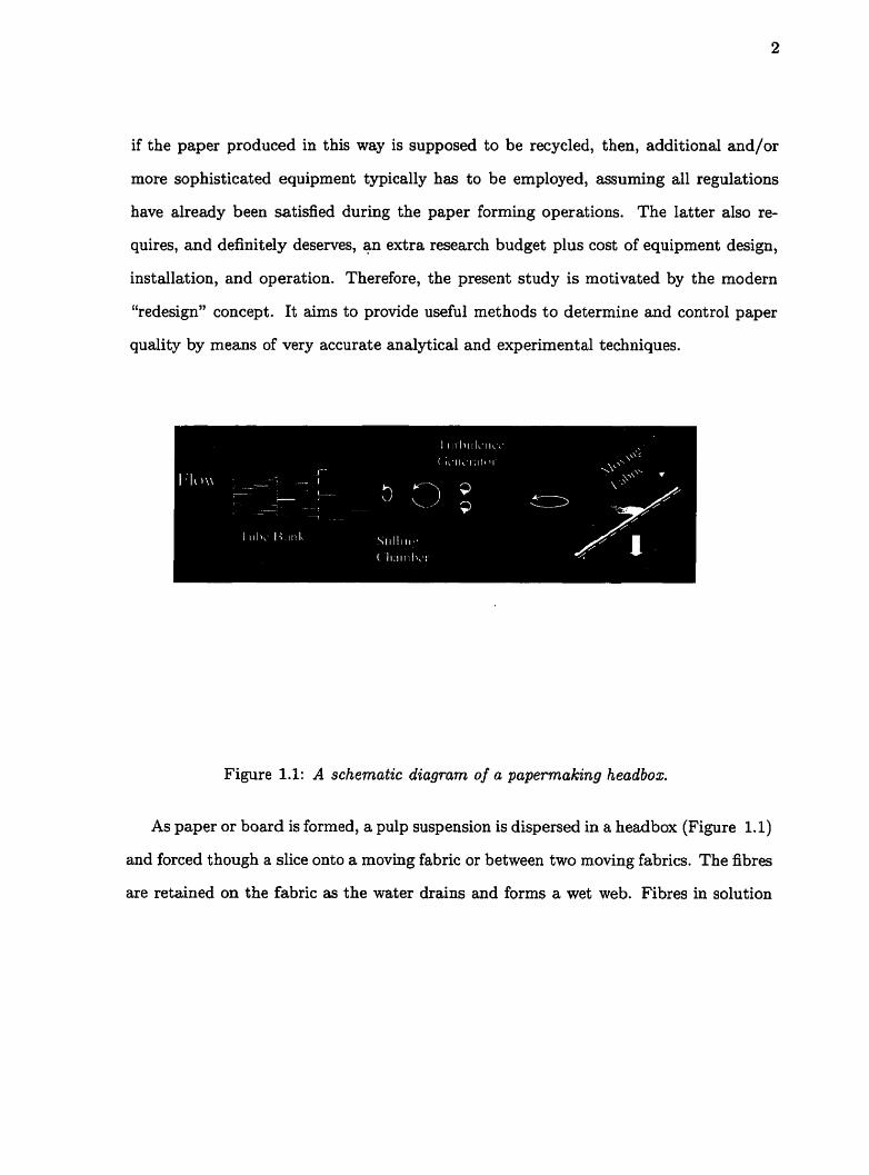
Figure 1.1: A schematic diagram of a papermaking headbox.

As paper or board is formed, a pulp suspension is dispersed in a headbox (Figure 1.1)

and forced though a slice onto a moving fabric or between two moving fabrics. The fibres

are retained on the fabric as the water drains and forms a wet web. Fibres in solution

tend to aggregate and form flocs producing nonuniformities in the sheet. Hydrodynamic

forces may enhance or retard fibre flocculation, depending on the flow characteristics.

One of the objectives of this study is to identify the effect of different papermaking flows

on the fibre flocculation. To achieve a uniform spatial distribution of fibres, turbulence

is introduced into the suspension in the headbox by a series of diffusers. However, fibres

tend to re-flocculate quickly as turbulence decays. This leads to the second objective of

this study to quantify fibre flocculation.

Figure 1.2: A jet issuing from the slice of a headbox (courtesy of D.

www8.s ymputico. ca/denis. mondor).

Mondor,

The final quality of paper produced depends in part on the state of the jet issuing

from the slice of the headbox (see Figure 1.2). Common problems like streaky jet flow

and/or variability in velocity across the slice will cause poor paper formation. The origin

of streaks is attributed to flow characteristics inside the headbox. However, direct floccu-

lation measurement in the headbox is extremely difficult. Computational fluid dynamics

(CFD) offers an alternative solution to this problem. It can be used as a guide to design

and modify pre-existing equipment. This thesis presents a fundamental guideline along

with experimental data for modeling fibre flocculation using commercially available CFD

packages.

The local mass variability or flocculation intensity and the scale for which this vari-

ability occurs (floc size distribution) generally characterize the quality of a sheet of paper.

The same principle applies to the case of a flowing pulp suspension. These quality pa-

rameters are studied both in the machine direction (MD) and cross machine direction

(CD). Figure 1.3 shows the arrangement of a scanner for CD and MD measurements and

connected manual process control device. The final objective of this work is to present

a model for characterizing MD and CD floc size distributions in suspension flows. The

motivation is to provide fundamental information for on-line monitoring and automatic

control of suspension, quality.

In summary the objectives of this study are:

Develop a system to measure mass variability in a grid generated turbulence flow

field.

Relate transverse and longitudinal mass variability of a flowing pulp suspension to

the mean flow velocity, mean concentration, and local flow field.

0 Develop models which describe the structure of fibre flocs and floc size distributions

in suspension flows.

A general literature review is presented in Chapter 2. It begins with the basic fluid

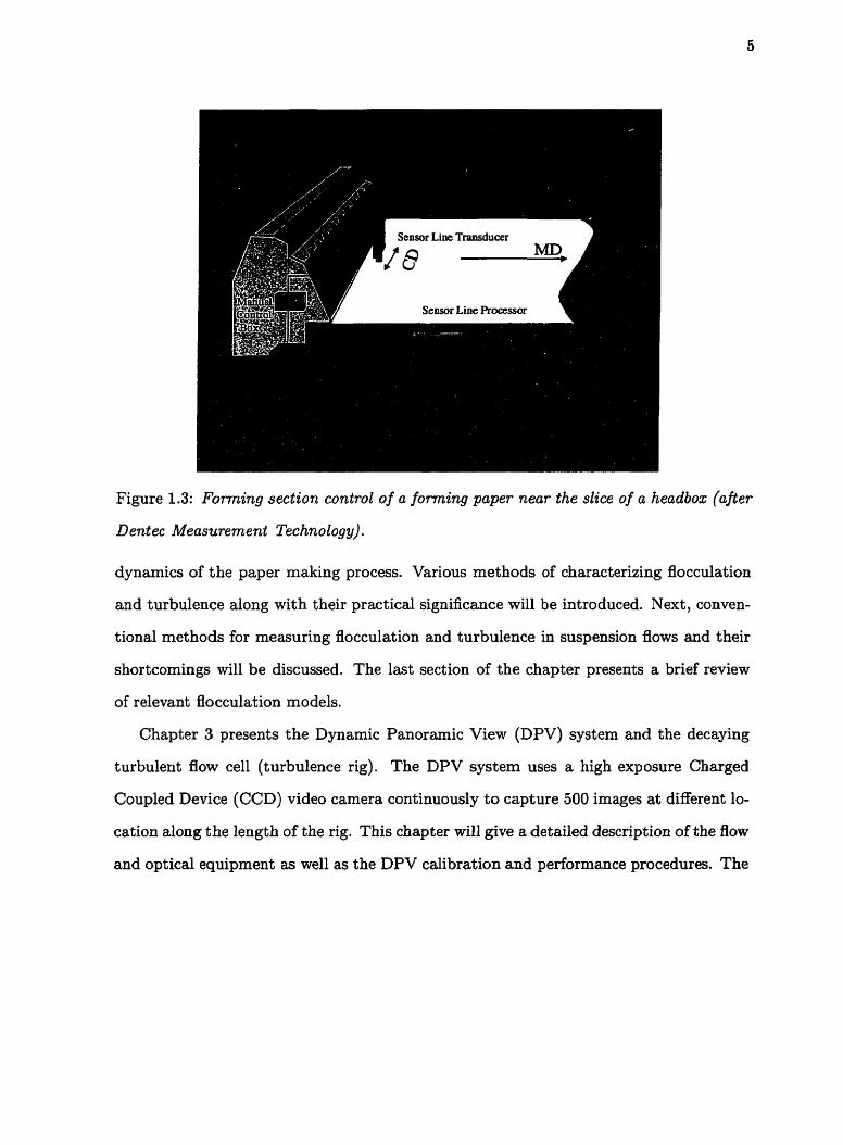
Figure 1.3: Forming section control of a forming paper near the slice of a headbox (after

Dentec Measurement Technology).

dynamics of the paper making process. Various methods of characterizing flocculation

and turbulence along with their practical significance will be introduced. Next, conven-

tional methods for measuring flocculation and turbulence in suspension flows and their

shortcomings will be discussed. The last section of the chapter presents a brief review

of relevant flocculation models.

Chapter 3 presents the Dynamic Panoramic View (DPV) system and the decaying

turbulent flow cell (turbulence rig). The DPV system uses a high exposure Charged

Coupled Device (CCD) video camera continuously t o capture 500 images at different lo-

cation along the length of the rig. This chapter will give a detailed description of the flow

and optical equipment as well as the DPV calibration and performance procedures. The

chapter will continue with the description of the statistical criteria, computer programs,

and image analysis associated with local mass variability measurement.

The application of the DPV system to the behavior of a hardwood semi-bleached fibre

suspension behind a grid generated turbulence flow field is presented in Chapter 4. A

general review of previous research and the motivation of the present study are discussed.

Fibre characteristics and measurement procedures are then presented. The presentation

of results and discussions begins with a qualitative description of the flow and follows

with the MD and CD flocculation intensity profiles, parametric studies of the effect of

bulk quantities (mean concentration and flow velocity), and finally characterization and

modeling of the flocculation intensity in the decaying turbulent field downstream of the

grids.

Cha,pter 5 presents a statistical model of floc size distribution in turbulent flow and

is divided into three sections. Following the first introductory section, a transverse floc

size distribution model will be developed, results presented and verified by experimental

data and well-established Richardson diffusion theory. The third section develops a

longitudinal floc size distribution model based on local Eulerian point measurement of

floc size distribution. The model predictions are compared with the measured floc size

distributions of hardwood and softwood species at different pulp consistencies.

Chapter 6 presents the conclusions and recommendations.

Chapter 2

Literature Review

Flocculation and dispersion of papermaking fibres have attracted attention of many

researchers since the late 1930s (see e.g. Wollwage 1939). Parameters affecting fibre

flocculation are numerous. Different researchers have investigated the fibre flocculation

phenomenon by considering either the physical chemistry of the problem (for an excel-

lent review of the literature see Chatterjee 1995) or the purely physical behavior of a

pulp suspension. Mason (1948) identified the mechanical entanglement of fibres as the

main cause of flocculation. Kerekes et al. (1985) later classified four types of cohesive

forces contributing to fibre flocculation: colloidal, mechanical entanglement, interface

frictional resistance, and surface tension. Extensive research by Swedish scientists (see

e.g. Norman et al. 1978) has been devoted to equipment design and measurement tech-

niques of pulp suspension flows. The present research is concerned with the (statistical)

physics and the fluid dynamics of suspension flows. With that regard, the previous

research will be reviewed in the sections that follow.

2.1 Pulp Flow Characteristics

2.1.1 Fully Developed Flows

Pipe flow is a typical example of a fully developed flow used in papermaking processes.

According to Norman et.al. (l978), due to the simple axi-symmetric geometry of a pipe

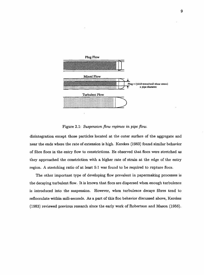
flow, most experimental research has focused on this type of flow. These authors have

explained three different types of suspension flows in pipes: Plug, mixed, and turbulent

flows (see Figure 2.1). At low Reynolds numbers, the fluid shear stress is not enough

to disrupt the fibre network, and the suspension flows as a plug. Increasing mean flow

velocity results in a hollow cylindrical layer of water in proximity of the pipe wall where

the fluid shear is maximum. The core region is however occupied by an intact plug. This

type of flow is referred to as mixed flow. At high mean flow velocity the core plug would

vanish as the fluid shear stress becomes higher than the fibre network yield stress, and

fibres in the suspension move erratically giving rise to a turbulent flow condition.

2.1.2 Developing Flows

According t o Tam Doo et al. (1984), fully developed flows may not be applicable for most

practical flows in papermaking processes. Examples include flows through rectifiers,

pressure screens, flow distributors, and headbox slices. These authors provided two

general characteristics for developing flows: shear and elongational flows. In an earlier

investigation, Kao and Mason (1975) compared two mechanisms of dispersion of non-

cohering plastic spheres in a Couette type device. They found that particle aggregates

within a rotational flow field move integrally around the same orbit with no sign of

Plug Flow

Mixed Flow

Turbulent Flow

Figure 2.1: Suspension flow regimes in pipe pow.

disintegration except those particles located a t the outer surface of the aggregate and

near the ends where the rate of extension is high. Kerekes (1983) found similar behavior

of fibre flocs in the entry flow to constrictions. He observed that flocs were stretched as

they approached the constriction with a higher rate of strain a t the edge of the entry

region. A stretching ratio of a t least 5:l was found to be required to rupture flocs.

The other important type of developing flow prevalent in papermaking processes is

the decaying turbulent flow. It is known that flocs are dispersed when enough turbulence

is introduced into the suspension. However, when turbulence decays fibres tend to

reflocculate within mili-seconds.. As a part of this floc behavior discussed above, Kerekes

(1983) reviewed previous research since the early work of Robertson and Mason (1956).

The application and use of decaying flows will be discussed in detail later in Chapter 4.

In the next section characteristics of a decaying turbulent flow downstream of a grid is

discussed.

2.2 Characteristics of Decaying Turbulent Flows

2.2.1 Decay of Kinetic Energy

The design of turbulent generators in papermaking headboxes has a great influence on

the dispersion of fibre aggregates. Most common turbulence generators include screens,

grids, and tube bundles (Ilmonniemi et al. 1986). There are three regions downstream

of the grid. The first is the developing region nearest the grid where the wake flows are

emerging, where the flow is inhomogeneous and anisotropic and there is a production

of turbulent kinetic energy. This region is followed by the second one where the flow

is nearly homogeneous and (locally) isotropic ' and where there is energy transfer from

larger eddies to smaller ones. The final decay of turbulence is the last stage of the decay

process furthest downstream from the grid, the flow is isotropic and homogeneous, and

viscous effects dominantly drain turbulent kinetic energy. Extensive experimental studies

in wind tunnels or water tunnels (Gad-El-Hak and Corrsin 1974, Roach 1986, Mohamed

and LaRue 1990) as well as theoretical treatment (see e.g. Hinze 1975) suggest that

the turbulence energy, d2 in the downstream of a grid, screen, etc., where turbulence is

more likely homogeneous and isotropic (the second region), decays as xn, where x isthe

'Turbulence is defined as isotropic if the statistical measures of flow are invariant to reflection and

rotations about all axes (Hinze 1975).

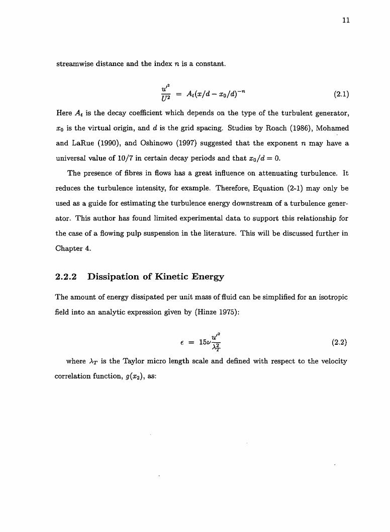
streamwise distance and the index n is a constant.

Here At is the decay coefficient which

At (x /d - xo/d)-" (2.1)

depends on the type of the turbulent generator,

$0 is the virtual origin, and d is the grid spacing. Studies by Roach (1986), Mohamed

and LaRue (1990), and Oshinowo (1997) suggested that the exponent n may have a

universal value of 10/7 in certain decay periods and that xo/d = 0.

The presence of fibres in flows has a great influence on attenuating turbulence. I t

reduces the turbulence intensity, for example. Therefore, Equation (2-1) may only be

used as a guide for estimating the turbulence energy downstream of a turbulence gener-

ator. This author has found limited experimental data to support this relationship for

the case of a flowing pulp suspension in the literature. This will be discussed further in

Chapter 4.

2.2.2 Dissipation of Kinetic Energy

The amount of energy dissipated per unit mass of fluid can be simplified for an isotropic

field into an analytic expression given by (Winze 1975):

where AT is the Taylor micro length scale and defined with respect to the velocity

correlation function, g ( x 2 ) , as:

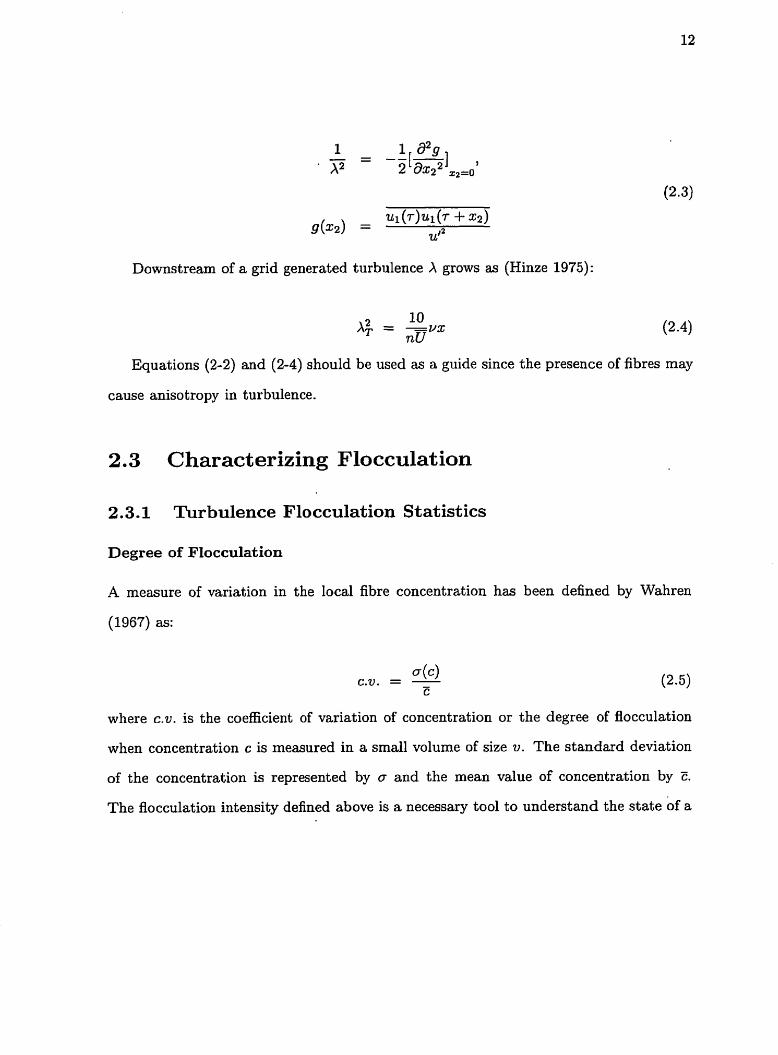
Downstream of a grid generated turbulence A grows as (Hinze 1975):

Equations (2-2) and (2-4) should be used as a guide since the presence of fibres may

cause anisotropy in turbulence.

2.3 Characterizing Flocculation

2 .%I Turbulence Flocculation Statistics

Degree of Flocculation

A measure of variation in the local fibre concentration has been defined by Wahren

(1967) as:

a (4 C.V. = - E

where C.V. is the coefficient of variation of concentration or the degree of flocculation

when concentration c is measured in a small volume of size v. The standard deviation

of the concentration is represented by a and the mean value of concentration by F.

The flocculation intensity defined above is a necessary tool to understand the state of a

pulp flow. For a well-dispersed suspension, the fluctuating concentration have a small

magnitude and hence the c.v is low. A flocculated suspension, on the other hand, should

exhibit a large fluctuation in concentration resulting in a higher value for c.v.

Scale of Flocculation

Analogous to the point correlations in turbulence, many researchers (Anderson 1966,

Norman and Wahren 1972, Persinger and Meyer 1975) have defined scale of flocculation

via different correlation functions. The two most common correlation functions are:

1. Longitudinal Correlation.

Persinger and Mayer (1975) used the auto-correlation function to determine lon-

gitudinal flocculation scale. This function defines the correlation between the

concentration fluctuations measured a t one point but a t different time intervals,

and is obtained from the following equation:

where the overbars represent the statistical average over time and cr denotes the

concentration fluctuation, which by definition: c = E + c'. Under Taylor's frozen

turbulence assumption the authors used the auto-correlation function to define

the macro scale of flocculation as:

2According to Hinze (l975), only if a homogeneous field has a constant mean velocity, oz = constant.,

then space and time has an approximate linear relationship.

or by virtue of a space correlation function (Norman and Wahren 1972) defined

as:

the flocculation macro length scale is then calculated as LC = S,OO f,(x)dx. Ac-

cording t o Norman and Wahren (1972) LC is the measure of the largest fibre flocs

occurring in a flowing pulp suspension. They attributed the micro length scale

A,, defined below, as the smallest eddies responsible for the dissipation of kinetic

energy as heat.

2. Cross Correlation

Evidently, a single dimension for fibre flocs defined above as LC may not adequately

describe the scale of flocculation in a suspension flow. In reality, fibres and flocs

flow in a 3-D flow field. Many other correlations may exist between two points

across the main flow direction, i.e. the y - direction. Persinger and Mayer (1972)

were the first who attempted to define a cross-correlation function for a suspension

flowing in a pipe. They proposed that the radial dimension of flocs can be obtained

from the following equations:

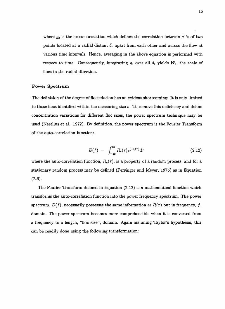
where gc is the cross-correlation which defines the correlation between c' 's of two

points located a t a radial distant 6, apart from each other and across the flow at

various time intervals. Hence, averaging in the above equation is performed with

respect to time. Consequently, integrating g, over all 6, yields W,, the scale of

flocs in the radial direction.

Power Spectrum

The definition of the degree of flocculation has an evident shortcoming: It is only limited

to those flocs identified within the measuring size v. To remove this deficiency and define

concentration variations for different floc sizes, the power spectrum technique may be

used (Nerelius et al., 1972). By definition, the power spectrum is the Fourier 'Ikansform

of the auto-correlation function:

E ( f ) = Jrn ~ , ( r ) e ( - ~ ~ ' ) d ~ (2.12) -00

where the auto-correlation function, RC(r), is a property of a random process, and for a

stationary random process may be defined (Persinger and Meyer, 1975) as in Equation

(2-6).

The Fourier Transform defined in Equation (2-12) is a mathematical function which

transforms the auto-correlation function into the power frequency spectrum. The power

spectrum, E( f ) , necessarily possesses the same information as R(T) but in frequency, f ,

domain. The power spectrum becomes more comprehensible when it is converted from

a frequency to a length, "floc size", domain. Again assuming Taylor's hypothesis, this

can be readily done using the following transformation:

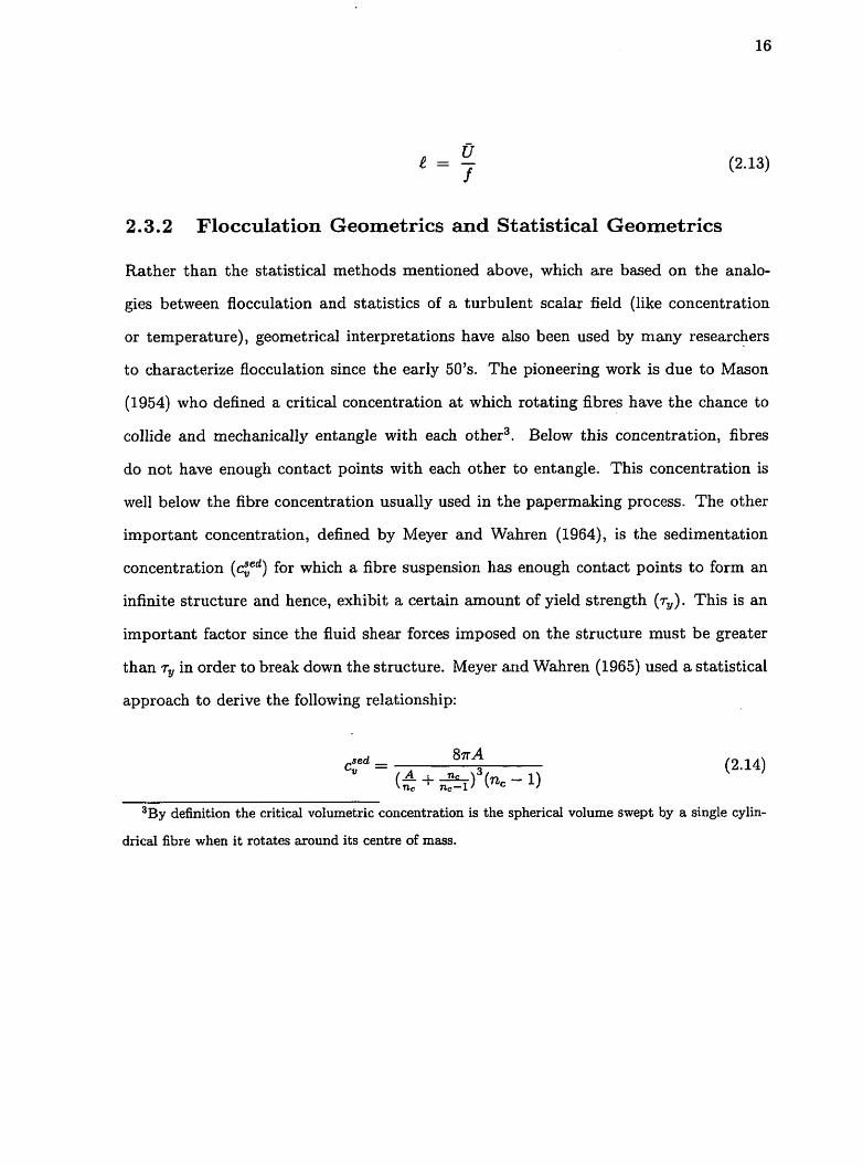
2.3.2 Flocculation Geornetrics and Statistical Geornetrics

Rather than the statistical methods mentioned above, which are based on the analo-

gies between flocculation and statistics of a turbulent scalar field (like concentration

or temperature), geometrical interpretations have also been used by many researchers

to characterize flocculation since the early 50's. The pioneering work is due to Mason

(1954) who defined a critical concentration a t which rotating fibres have the chance to

collide and mechanically entangle with each other3. Below this concentration, fibres

do not have enough contact points with each other to entangle. This concentration is

well below the fibre concentration usually used in the papermaking process. The other

important concentration, defined by Meyer and Wahren (1964)' is the sedimentation

concentration (cd,Cd) for which a fibre suspension has enough contact points to form an

infinite structure and hence, exhibit a certain amount of yield strength (7.). This is an

important factor since the fluid shear forces imposed on the structure must be greater

than in order to break down the structure. Meyer and Wahren (1965) used a statistical

approach to derive the following relationship:

3By definition the critical volumetric concentration is the spherical volume swept by a single cylin-

drical fibre when it rotates around its centre of mass.

where n, and A represent the number of fibre/fibre contacts per fibre and fibre aspect

ratio, i.e. the ratio of the fibre length to its width, respectively, Kerekes et-al. (1985)

extended Mason's argument and defined the "crowding number" as the number of fibres

inside of a spherical volume of diameter equal to a fibre length:

Kerekes and Schell (1992) used the crowding number to characterize the uniformity

of a flowing pulp suspension passing through a grid-plunger device. Working with mass

concentration, C,, instead of c, appears to be more convenient. Therefore, Dodson and

Schaffnit (1992) proposed:

where X and 6 represent the fibre length

ness) , respectively. Soszynski and Kerekes

and mass of a fibre per unit length (coarse-

(1988) characterized the state of fibre sus-

pensions with respect to n,,,d. Fibres undergo a chance collision in dilute suspension

when n,,,d < 1, force collision in semi-concentrated suspension when 1 < n,,,d < 60,

and continuous contact in concentrated suspension when n,,d > 60. The crowding

number in a typical stock of a papermaking headbox lies in the range 10 < n,,,d < 45

(Kerekes 19%).

An important statistical geometric (Deng and Dodson 1994) element of a fibre net-

work is the fibre-fibre gap lengths. This characterizes the pore structure of the network.

Corte and Lloyd (1965) proposed a negative exponential distribution for the gap length

in paper as a result of random spatial distribution of fibres. Dodson and Sarnpson (1996)

proposed the Gamma distribution for the gap lengths to be used. for the case of non-

random (flocculated or dispersed) sheets. The gap distribution in fibre suspensions will

be discussed in detail in Chapter 5.

2.4 Measurement Techniques

2.4.1 Flow Measurements

Laser Doppler Anemometry (LDA) is a non-intrusive technique for measuring local tur-

bulent velocity. In this technique two laser beams are brought together to form a fringe

pattern at their ellipsoidal intersection area. When a passive particle (an inert particle)

in the flow passes through this area it scatters the light pulses at a certain frequency f .

The scattered light pulses are detected by an electronic device and the corresponding

frequency is measured and the flow velocity is calculated from the following equation:

f t d u=- 2 sin f

where td is the laser wavelength and B is the angle between the two laser beams. Kerekes

and Garner (1982) used this technique to estimate the grid generated turbulent charac-

teristics of a flowing pulp suspension. However, their result was found to be ambiguous;

since it was not clear whether the measured velocities were of the passive particles or

fibres. To eliminate the measurement ambiguities associated with the high frequency

fluctuations, d'Incau used a low-pass filter and smoothed out the output signals. Steen

(1989) performed LDA measurement in a refractive index matched solution to eliminate

the light scattered due to the presence of fibres.

More advanced techniques like Particle Image Velocimetry (PIV) (Adrian 1991) are

currently being used to measure turbulence characteristics a t the Pulp and Paper Centre,

University of Toronto. PIV has a great advantage over LDA as it can measure the

simultaneous velocity of thousands of points over a plane of field a t once.

2 A.2 Flocculation Measurements

According t o Norman et-al. (1978), mean and fluctuating concentrations can be mea-

sured using the optical properties of the fibres. The optical configurations were generally

categorized into two techniques: Light transmission and Light reflection. According to

Bakker et.al. (l994), optical methods may be broken down into two general classes: One

produces a tunnel vision and the other a panoramic view. The former measures the point-

to-point properties of a concentration field whereas the other instantaneously monitors

thousands of point information over a well-defined measurement area. The latter has su-

periority specially when one needs to perform space/time-correlation analysis associated

with Equation (2-10).

Light Reflection

Impact probes (see Figure 2.2) have been used in the past t o obtain the degree of

flocculation and flocculation power spectrum (Nerelius et al. 1972). The probes include

two light guides. Incident light from a light guide with an effective diameter of about

1.5mm is partially reflected after hitting a bundle of moving fibres and passed through

the other Iight guide. A photo diode converts the light energy into a current which

is amplified and converted to a voltage. A RMS meter determines the variation in

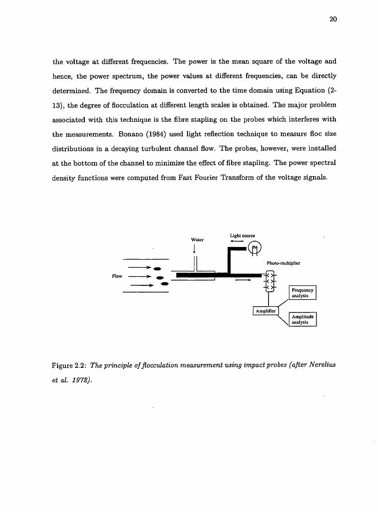
the voltage a t different frequencies. The power is the mean square of the voltage and

hence, the power spectrum, the power values at different frequencies, can be directly

determined. The frequency do~ilain is converted to the time domain using Equation (2-

13), the degree of flocculation at different length scales is obtained. The major problem

associated with this technique is the fibre stapling on the probes which interferes with

the measurements. Bonano (1984) used light reflection technique to measure floc size

distributions in a decaying turbulent channel flow. The probes, however, were installed

a t the bottom of the channel to minimize the effect of fibre stapling. The power spectral

density functions were computed from Fast Fourier Transform of the voltage signals.

-0

Flow .-------) * - 0

Light source Wnter - A

JS3L Fl analysis

Amplifier Amplitude

Figure 2.2: T h e principle of ~ o c c u l a t i o n measurement using impact probes (after Nerelzus

e t al. 1972).

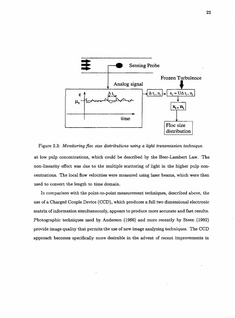
Light Transmission

In a light transmission technique, incident light of either a laser beam or a white light

is used to illuminate a small area of a flowing pulp suspension. According to the Beer-

Lambert law, the transmitted light is exponentially proportional to the pulp concentra-

tion. Hourani (1989) used this approach as illustrated in Figure 2.3 to obtain point-

to-point measurements of floc size distributions of a flowing pulp suspension. A small

illuminated portion of the suspension is sensed by a photo diode through which the

fluctuations in voltage, caused by variations in concentration over a certain period of

time, are collected. The mean voltage is then calculated and two consecutive crossings

between the mean and the voltage function is defined as a floc size. The time domain

of the function is converted to the length domain using the Taylor frozen turbulence

hypothesis and a floc size distribution is determined.

According to Norman and Wahren (1972), the total number of crossings per unit

time, No, may be used to determine the micro length scale using the folowing equation:

This is a simple method of estimating A,, since there is no need to determine experi-

mentally the auto-correlation function, as would be required by the method associated

with Equation (2-9). Takeuchi et al. (1983) used a He-Ne laser beam as the incident

light source to illuminate an area of about 0.8 mm2 area and measured the intensity

of the transmitted light using a photo-multiplier. The fluctuating light intensity caused

by local variations in concentration is then analyzed using a spectrum analyzer. The

relationship between the transmitted light and pulp concentration is established through

a calibration procedure. The authors found that this relationship was not linear, except

Sensing Probe

Frozen Turbulence Analog signal

* time

FIoc size distribution

Figure 2.3: Monitoring ftoc size distributions using a light transmission technique.

a t low pulp concentrations, which could be described by the Beer-Lambert Law. The

non-linearity effect was due t o the multiple scattering of light in the higher pulp con-

centrations. The local flow velocities were measured using laser beams, which were then

used to convert the length to time domain.

In comparison with the point-to-point measurement techniques, described above, the

use of a Charged Couple Device (CCD), which produces a full two dimensional electronic

matrix of information simultaneously, appears to produce more accurate and fast results.

Photographic techniques used by Anderson (1966) and more recently by Steen (1992)

provide image quality that permits the use of new image analyzing techniques. The CCD

approach becomes specifically more desirable in the advent of recent improvements in

computer technology (Jahne 1997). The higher order statistics as well as simultaneous

time-space correlations, which reveal more detailed information about the state of fibre

flocculation in turbulent flows, may now be obtained with an acceptable accuracy and

much faster than the conventional point-to-point vision techniques. A new "panoramic

view" technique that takes advantage of these technical advancements has been devel-

oped for flocculation measurement and is presented in the next Chapter.

2.5 Modeling Fibre Flocculation

Few researchers have attempted to model flocculation in turbulent flows. Pioneering

work is due to Mason (1950) who proposed the frequency of fibre collisions per unit

volume per unit time, vc, in a dilute suspension subject to a simple shear field. It is

given by:

In this equation Np is the number of particles per unit volume, j shear rate, v volume

of a single particle. According to Mason, this equation may also be used for turbulent

flows. Steen (1990) proposed a more complicated model for fibre flocculation in turbulent

flows. In his model the rate of aggregation is proportional to the floc concentration and

fibre concentration. Anderson (1964) proposed a floc break-up model that implies the

scale of flocculation is inversely proportional to the turbulent kinetic energy and directly

to the mean consistency.

Hourani (1988) used a statistical thermodynamic approach to model fioc size dis-

tributions. His model has two unknown parameters, which have to be obtained from

experiments. Hourani linked the proposed floc size distribution to a two-phase isotropic

turbulence flow field using the assumption that the mean floc size is equal to the mean

eddy size. This model will be rigorously analyzed in Chapter 5.

Chapter 3

Experimental Design and

Methodology

A flow loop system was constructed to study turbulent fibre flocculation for the purpose

of advancing knowledge of the behavior of pulp suspension in a decaying turbulent flow

field. This chapter introduces the experimental technique developed in this study. The

instrumentation and apparatus utilized, and the experimental methodology used for

flocculation measurement will be discussed in detail. The first section of this chapter

will describe the flow loop designed for generating a turbulent flow field. The second

section will describe the development of a Dynamic Panoramic View (DPV) system

used to measure turbulence flocculation. The DPV performance and calibration will be

discussed in the third section. The application of DVP to measuring flocculation will be

presented in the last section.

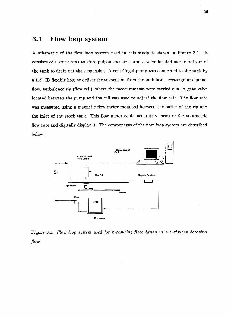
3.1 Flow loop system

A schematic of the flow loop system used in this study is shown in Figure 3.1. It

consists of a stock tank to store pulp suspensions and a valve located at the bottom of

the tank to drain out the suspension. A centrifugal pump was connected to the tank by

a 1.5" ID flexible hose to deliver the suspension from the tank into a rectangular channel

flow, turbulence rig (flow cell), where the measurements were carried out. A gate valve

located between the pump and the cell was used to adjust the flow rate. The flow rate

was measured using a magnetic flow meter mounted between the outlet of the rig and

the inlet of the stock tank. This flow meter could accurately measure the volumetric

flow rate and digitally display it. The components of the flow loop system are described

below.

PC & AcquLriliun Cnnl

CCD HiJlSpcal V i h Camem

,..*................................................... . .... . ...... ...,...

- NOW CCII ~ a g n c ~ i c ~ I I W Mclcr

v -

i f lmf im

Figure 3.1: Flow loop system used for measuring flocculation in a turbulent decaying

Bow.

1. Stock tank with a capacity of 24 Litres.

2. Centrifugal pump with a capacity of 3000 Lit/hr.

3. Flow Cell. A turbulence rig (flow cell), shown in Figure 3.2, consisted of two main

sections: A vertical entry flow channel, normal to the main flow, and a horizontal

rectangular channel. Therefore, the rig utilized a sudden sharp bend (90 degree)

section a t the entrance to disperse, then deliver a fibre suspension evenly across

the width of the horizontal channel. Different types of suspension distributors were

initially designed and tested. These are shown in Figure 3.3. A circular diffuser

(type A) connected to the inlet of the horizontal channel produced an asymmetric

flow. Rectangular grids were introduced a t the entrance of the horizontal channel

to disrupt the asymmetric flow, but did not produce a uniform flow (Type B). Type

C used cylindrical bars as a turbulence generator but fibres stapled on the bars

and blocked the flow. In the L-type the fibre suspension was first forced to pass by

the vertical channel and then i t turned into the vertical channel. The suspension

was highly mixed a t the turning point and evenly distributed over the width of

the horizontal channel. An erratic motion of the dispersed fibres was observed

near the entrance of the horizontal channel. At a distance 50 cm downstream of

the entrance just before the grids, the suspension flow was fully developed with no

relative motion of fibres. In this manner the L-type distributor was found to be

superior than the others.

4. Flow Meter. The flow rate of pulp suspension was measured by a ECOFLUX

10 1 OK/D6 compact electromagnetic flow meter made by KROHNE and specifically

Figure 3.2: Geometry of the flow cell used for generating turbulent decaying f i w field.

designed for pulp suspension flows. This flow meter works based on Faraday's law

of induction. Thus, it is designed for an electrically conductive fluid. When the

suspension with a mean velocity flows perpendicular t o the direction of a high

magnetic field of strength, B, an electric voltage is generated which depends on its

velocity. This voltage signal is converted to a digital signal and, the magnitude is

displayed on the instrument screen. The following equation is used for correlating

the voltage induced and the flow velocity.

where B, D4, and K, are the voltage, pipe diameter, and a calibration constant,

respectively.

5. Valves. A gate valve, installed between the flow cell entrance and the pump, is

Figure 3.3: Flow distributors and corresponding flow patterns produced by them .

used for adjusting the flow rate. A gate valve is installed a t the bottom of the

stock tank to drain the pulp suspension after each experiment.

3.2 Elements of the Dynamic Panoramic View Sys-

tem

A schematic diagram of the optical system and work station used for flocculation mea-

surement is shown in Figure 3.4. A Tungsten diffuse-backlight source was used for

illuminating an effective area of 23mm x 20mm of a moving pulp suspension. The light

intensity was controlled by adjusting the output current of a 110v/7.5v transformer.

An AC/DC converter, which was connected to the transformer, was used to produce a

non-flickering light. The light source, which was positioned under the flow cell, had a

focusing lens system to achieve a highly intense light area. A CCD video camera was

used to capture images of the flowing suspension a t different locations of the cell. The

Monitor A displayed these images and was used for visual quality control. A frame

grabber located inside of a Pentium PC digitized the output analog signals from the

camera. The digitized data were saved to hard disc memory of the PC then transmitted

to a Unix machine for analysis. The following items explain the components of the DPV

system in detail.

Video Micrometer ,,,

~entiun 200. Image Digitizer, Win 3.1 & Par Software

Flow Cell I Diffwer

Light Source

24 " Long Rack & Pinion Slide for Precise Positionin

Figure 3.4: A schematic diagram of the imaging system facilities and set-up used for

flocculation measurements.

CCD video camera

A black and white Charged Coupled Device (Optikon Ltd.) video camera was positioned

above the flow cell and in front of the light source to capture the images of the flowing

suspension a t a rate of 30 frames/sec. The camera had a sensor area of 8.3mm x 6.3mm

with an effective pixels resolution of 752 (Horizontal) x 480 (Vertical). The exposure

time of the camera could be set as low as lpsec. In the present work, the exposure time

was found to be in the range of 150-300 psec.

Optical system

A 55mm Telecentric lens (Computar 55, Edmund Scientific) together with a 0.75X ex-

tension lens and 16 mm extension tube were used to view an area of 33.3mm x 24.9mm.

Figure 3.5 shows the main function of the Telecentric lens on mapping objects onto

their images. I t basically minimizes uncertainties associated with the viewing angle and

image magnification. Typically, the error in the image scale is about 1% at a f 12.4 mm

object movement and 0.5X magnification. An approximation of the depth of field, DoF,

associated with the required optics is given by (see Smith 1990 , Jahne, 1997):

where, fnzLmber is defined as the ratio of the lens focal length and the aperture diameter, M

is the lens magnification, defined as image size object size and d, is a parameter that characterizes the

sharpness of the image. To achieve the best sharpness, any point in the measuring volume

is mapped onto a disk with diameter d,. Based on Equation (3-2), a t magnification

Ad = &- = 0.251, fmmber = 11, and dc = 34pn (defined for the two adjacent

pixels on the sensor) the depth of field would be DoF = f 4.5mrn. In practice, images

taken of the fibre suspension in the flow cell were found to be adequately sharp even at

a larger DoF x f5.5mm. This value for the depth of field corresponds to the thickness

of the flow cell.

Figure 3.5: Top view of nine identical cylinders with an angular viewing error ( top) and

with a telecentric view (bottom).

3.2.1 Video Micrometer

The output analog signal of the CCD video camera was sent to a video micrometer

(XR 2000-Micrometer, Edmund Scientific) through which the location and size of the

images were accurately controlled. The device was set to depict a rectangular frame of

size 23mm x 20mm on Monitor A, as shown in Figure 3.6, as the reference area. The

pre-designed zones of measurements, which were printed on a transparency, were fixed

on the cell wall at different locations, see Figure 3.7. The position of the camera was ad-

justed such that the zones of measurements, image windows, superimposed the reference

window. As will be discussed latter, this equipment saved a great deal of computational

time for determining the boundaries of images and improves the reproducibility of the

experiments.

11 Black Frame: Image Window

White Frame: Reference Window

Image Area

Figure 3.6: A measuremen.t area transposed by the reference window.

Flow

r) x-x- - -

Figure 3.7: Test section of the turbulence rig and measurement area used for fEocculation

measurements.

Image grabber

The DVP system used a TBC IV frame grabber (Digital Systems Inc.) to digitize the

analog signals from the camera. The interface device links the CCD camera to the

Pentium computer video system over a 16-bit expansion slot. Serial control data was

fed to the TBC card via the rear panel mini DIN-9 connector. The card obtained its

power from the expansion slot. A Personal Animation Recorder (PAR, DPS Inc.) card

was used to record and dynamically analyze of the captured images in real time. Due to

the limitation of the camera frame rate, the dynamic behavior of fibre suspension flows

was observable only at lower flow velocities.

Due to the massive amount of data, approximately 30Mb/sec per experiment, to

Table 3.1: Parameters of the Image Grabber. I I I I I I Image Format I Block Limit I Quality Factor I Color Mode 1 I 24bit TARGA, Field 1 300 1 17 I B/W Mono I

be digitized and converted to motion video in real time, PAR uses a MOTION JPEG

algorithm to compress and then decompress the data. The TBC and PAR devices are

controlled by two software packages that adjust and control system parameters, such

as Quality Factor, rate of compression, color adjustment (with RGB code) etc. The

adjusted parameters used in this study are listed in Table 3.1. The software programs

were executable within a Microsoft Win 3.1 environment.

Traversing mechanism

The camera and the illuminating light system were both connected to a rack and pinion

system (Edmund Scientific). The whole system could traverse the length of the flow

channel and be fixed at any distance downstream from the grids. In this manner the

effect of decaying turbulence on the flocculation was studied.

3.3 Imaging performance and calibration

3.3.1 CCD Camera performance

The vision performance of the CCD camera was investigated by imaging a well-defined

gray scale target. The target consisted of 5 strips of Mylar film in a slide form. Each

strip differed from the others only in density. The variation between densities was chosen

to be linear. Mylar was chosen due to its similar variation of density with gray level as

compared to cellulose.

Figure 3.8: Images of the background (bottom), Mylarji lm before (top) and a8er (middle)

the background cancellation operation.

0. 10 .OD

Scan Axis (Mylar Image)

Scan Axis (Corrected Mylar Image)

1 0 0 . . 100 ,#,a ma* .OD

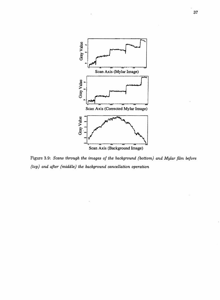
Scan Axis (Background Image)

Figure 3.9: Scans through the images of the background (bottom) and Mylar film before

(top) and after (middle) the background cancellation operation

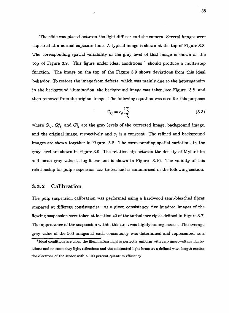
The slide was placed between the light diffuser and the camera. Several images were

captured a t a normal exposure time. A typical image is shown a t the top of Figure 3.8.

The corresponding spatial variability in the gray level of that image is shown at the

top of Figure 3.9. This figure under ideal conditions should produce a multi-step

function. The image on the top of the Figure 3.9 shows deviations from this ideal

behavior. To restore the image from defects, which was mainly due to the heterogeneity

in the background

then removed from

illumination, the background image was taken, see Figure 3.8, and

the original image. The following equation was used for this purpose:

where Gij , G!j, and G& are the gray levels of the corrected image, background image,

and the original image, respectively and c, is a constant. The refined and background

images are shown together in Figure 3.8. The corresponding spatial variations in the

gray level are shown in Figure 3.9. The relationship between the density of Mylar film

and mean gray value is log-linear and is shown in Figure 3.10. The validity of this

relationship for pulp suspension was tested and is summarized in the following section.

3.3.2 Calibration

The pulp suspension calibration was performed using a hardwood semi-bleached fibres

prepared a t different consistencies. At a given consistency, five hundred images of the

flowing suspension were taken at location 22 of the turbulence rig as defined in Figure 3.7.

The appearance of the suspension within this area was highly homogeneous. The average

gray value of the 500 images at each consistency was determined and represented as a

lIdeal conditions are when the illuminating light is perfectly uniform with zero input-voltage fluctu-

ations and no secondary light reflections and the collimated light beam at a defined wave length excites

the electrons of the sensor with a 100 percent quantum efficiency.

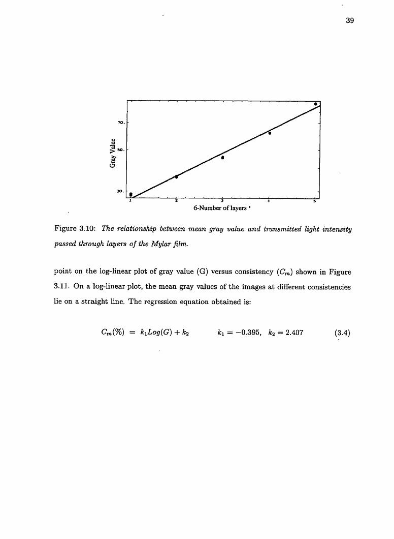
6-Number of layers '

Figure 3.10: The relationship between mean gray value and transmitted light intensity

passed through layers of the Mylar film.

point on the log-linear plot of gray value (G) versus consistency (C,) shown in Figure

3.11. On a log-linear plot, the mean gray values of the images at different consistencies

lie on a straight line. The regression equation obtained is:

0.3 0.4 0.5 0.6 0.7 0.8

Consistency, %

Figure 3.11: Calzbration curve for a hardwood semi-bleached fibre suspension.

3.4 Flocculation Measurements

The goal of this study was to measure the flocculation intensity of a flowing pulp sus-

pension in a decaying flow field. Flocculation measurements were performed over the

long rectangular central volume 300 mm (x-direction) x 15 mm (y-direction) x 11 mm of

the 125 cm x 15.2 cm x 1.1 cm turbulence rig (see Figure 3.7). To improve experimental

reproducibility of the measurement area a transparency with 13 marked measurement

zones was fixed at the top wall of the rig. The flocculation intensity at any location was

defined as:

where c and i? are the instantaneous and mean concentrations, respectively. Introducing

Equations (3-3) and (3-4) into Equation (3-5), yields for var:

- - var = ~ : ( ( L ~ ~ G o - L ~ G O ~ )

The contribution of the background noise and its interaction with the image is evident

from the last two terms on the right hand side of the Equation (3-6). For negligible noise,

Equation (3-5) and (3-6) reduce to:

The averaging operations involved with the above equations could only be carried out

if the total number of image samples Nf were known. The following section offers a

criterion to select Nf .

3.4.1 Number of Images

The number of images required for each experiment depends on the mean consistency,

flow velocity, flocculation intensity, and the expected accuracy of the measurements. The

sampling criteria used for flocculation measurements was similar to that of turbulence

measurements (Oshinowa 1996). The uncertainty in the measured mean consistency

within an accuracy +I%, based on a 99% confidence level, and subjected to a Gaussian

error, is:

where yp is the random variable of a standard Gaussian density function a t prob-

ability (1 - P ) , e[&] is the normalized rms and 0[6m] is the standard deviation of the

measured mean value em. The normalized error is given by

where Nf is the number of images and ( z ) ~ is the flocculation intensity. For a typical

value of flocculation intensity 0.008, we have

In the present work the number of images analyzed for each experiment was 500 fields

a t the same location.

3.4.2 Image Analysis

This section describes the procedures and algorithms that were developed to obtain

numerical values for the flocculation intensity from the images captured and stored in

the PC by the PAR system. A general perspective of routes developed for image analysis

is shown in Figure 3.12. As mentioned above, the TBC image digitizer and PAR system

collect color images by default. Since the CCD camera collects momochrome images,

these images were all set to be stored in monochrome RGB 24 bit format for which only

lMbyte of memory was required per image. The Mathernatica program img- manage.ma

was developed to convert the data color format to an 8-bit gray format and reduce the

size of each image. The program called C code subroutines (provided by PBMPLUS)

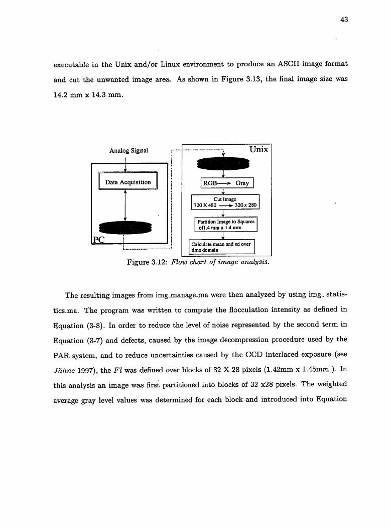
executable in the Unix and/or Linux environment to produce an ASCII image format

and cut the unwanted image area. As shown in Figure 3.13, the final image size was

14.2 mm x 14.3 mm.

Analog Signal

I Data Acquisition A

v

.-.-.-.-.-.-.-.-a-m---. Unix

Partition Image to Squares of1.4mmx 1.4mrn

Calculnte mean and sd over time domain

Figure 3.12: Flow chart of image analysis.

The resulting images from imgmanage-ma were then analyzed by using img- statis-

tics-ma. The program was written to compute the flocculation intensity as defined in

Equation (3-8). In order t o reduce the level of noise represented by the second term in

Equation (3-7) and defects, caused by the image decompression procedure used by the

PAR system, and to reduce uncertainties caused by the CCD interlaced exposure (see

Jiihne 1997), the F1 was defined over blocks of 32 X 28 pixels (1.42mm x 1.45mm ): In

this analysis an image was first partitioned into blocks of 32 x28 pixels. The weighted

average gray level values was determined for each block and introduced into Equation

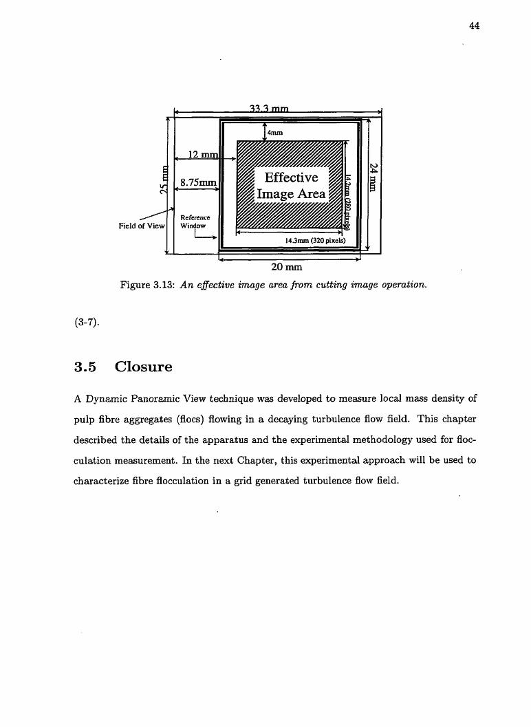
Reference Window

-11 ' 14.3mm (320 pixels)

Figure 3.13: An effective image area from cutting image operation.

3.5 Closure

A Dynamic Panoramic View technique was developed to measure local mass density of

pulp fibre aggregates (flocs) flowing in a decaying turbulence flow field. This chapter

described the details of the apparatus and the experimental methodology used for Aoc-

culation measurement. In the next Chapter, this experimental approach will be used to

characterize fibre flocculation in a grid generated turbulence flow field.

Chapter 4

Characterization of Fibre

Flocculation in Turbulent Decaying

Flows

4.1 Introduction

The final quality of the paper produced depends in part on the state of the jet issuing

from the slice of the papermaking headbox. The origin of common problems such as

streaky jet flow and/or variability in velocity across the slice that cause poor paper

formation has been studied extensively by numerous researchers. Wrist (1962) studied

the effect of perforated roller turbulence generators (see Figure 4.l)on jet stability and

observed that the closer the rollers were to the slice the more streaky the jet. He

attributed this variation to the high turbulence intensity produced near the holes of the

rollers. In his theoretical analysis, Van Den Akker (1954) suggested the distance between

Moving Fabric white water 1

Figure 4.1: A schematic diagram of a headbox with the rectz,fier roller turbulence gener-

ator.

the turbulence generator and the slice in a headbox should be as far apart as possible to

increase the homogeneity of turbulence at the slice. An increase in distance, however,

results in a lower turbulence intensity a t the slice and, hence, the reaggregation of the

fibres.

Parker (1968) postulated that optimal conditions in the converging exit channel of

the headbox, both in terms of floc dispersion and jet stability, are achieved by turbulence

generated with a small turbulence length scale of mild intensity. This is the basic concept

of low turbulence headboxes (Kerekes 1979) and in a wind tunnel may be achieved using

fine mesh screens, flow modifiers, grids, etc. (Roach 1986). Unfortunately, the wind

tunnel approach can not be directly applied to the case of pulp suspension flows, since

fibres will block the holes of the screen. Thus, Parker concluded that the determining

element for generating small-scale turbulence is the converging exit channel geometry

in the headbox. Kerekes (1983) observed that this approach to turbulence generation

has a significant shortcoming: small-scale eddies decay rapidly in pure water, and even

more rapidly in a fibre suspension. Therefore, there exists a compromise between the

jet quality and level of turbulence.

Ilmonniemi et. al. (1986) investigated the effect of various types of headbox turbu-

lence generators, as shown in Figure 4.2, on the jet stability and grammage uniformity.

From their results, a tube bunch turbulence generator, Type B in Figure 4.2, pro-

duces the most stable jet flow with a relatively lower turbulence intensity and small half

energy wavelength. Their results can only be used as a guide since their turbulence

measurements were for pure water only.

Several workers have attempted to measure pipe flow turbulence flocculation using

intrusive probes (see Sanders and Meyer 1971, Presinger and Mayer 1975, Nerelius et.

al. 1972). In this technique a sensor, e.g. a fibre optic, is inserted into the flow

and its response is characterized through calibration. It has three major shortcomings:

fibres stapling on the sensor, extensive calibration (Kerekes and Garner 1982), and

limitations in sensor size and configuration. Thus, for example, Persinger and Mayer's

(1975) measurements on radial scales of flocculation in a pipe flow were found to be

inconclusive.

Bonano (1984) studied the effect of high pulp concentration, i-e. 1 to 3 percent, and

mean velocity on flocculation in a decaying turbulent flow field using a light reflection

technique. Turbulence was generated by a gradual constriction (converging/diverging)

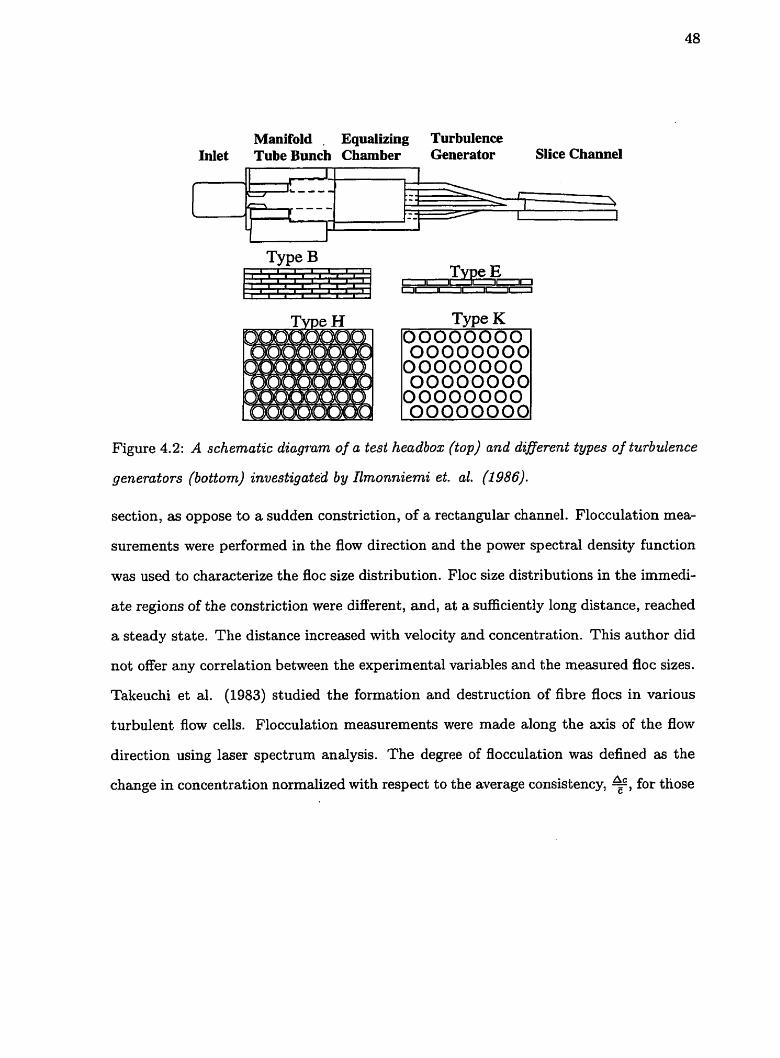
Manifold . Equalizing Turbulence Inlet Tube Bunch Chamber Generator Slice Channel

n I I

Figure 4.2: A schematic diagram of a test headbox (top) and different types of turbulence

generators (bottom) investigated by I l n o n n i e m i et. al. (1986).

section, as oppose to a sudden constriction, of a rectangular channel. Flocculation mea-

surements were performed in the flow direction and the power spectral density function

was used to characterize the floc size distribution. Floc size distributions in the immedi-

ate regions of the constriction were different, and, at a sufficiently long distance, reached

a steady state. The distance increased with velocity and concentration. This author did

not offer any correlation between the experimental variables and the measured floc sizes.

Takeuchi et al. (1983) studied the formation and destruction of fibre flocs in various

turbulent flow cells. Flocculation measurements were made along the axis of the flow

direction using laser spectrum analysis. The degree of flocculation was defined as the

change in concentration normalized with respect to the average consistency, 9, for those

flocs having the highest spectral density. They found that flocs were formed in decaying

turbulent flows and were destroyed in converging channel flows. They postulated that

the destruction of flocs was due to the shear stress imposed on the flocs by the channel

walls. In the converging flow channel, the flocs experienced an increasing shear stress

with downstream flow direction. They suggested that the shear stress became greater

than the fibre network yield stress and flocs ruptured, and hence, the level of flocculation

decreased.

Using high-speed cinematography, an extensive qualitative study was performed to

understand the formation of flocs in a turbulence decaying flow field (Kerekes 1983,

Kerekes et al. 1985). Turbulence was generated by a set of rectangular bars in a

rectangular channel. Kerekes observed that flocs, once they formed, may actually keep

their coherent structure in the transient and/or final decay of turbulence (Batchelor and

Townsend 1948).

A recent trend in the study of turbulence and flocculation in headboxes is the use

of Computational Fluid Dynamics (CFD) (see f.g. Lee and Majumdar 1979, Jones and

Ginnow 1988, Steen 1989, and Aiden 1996). In this work, there has been an attempt to

produce correlations through which the local fluctuations in concentration is character-

ized by bulk quantities. With limited success, Steen (1989) numerically modeled fibre

flocculation by assuming the flocculation intensity is conservable.

In the present study, a flow channel was designed to quantify experimentally the

effect of bulk flow velocity and concentration on the flocculation intensity in a turbu-

lent decaying flow field behind parallel grids. The definition of flocculation intensity as

the temporal mass variability is a simple yet extremely useful way of representing data

for two reasons: It is in complete analogy with turbulence intensity measurement and

provides a tool for the mechanistic modeling of turbulence flocculation through conser-

vation of flocculation intensity. The aim of this work is to characterize flocculation with

respect to flow velocity and pulp consistency, analogous to the characterization of the

turbulence intensity.

4.2 Experiment a1

4.2.1 Material

All experiments in this study used never-dried semi-bleached hardwood kraft pulp. The

physical characteristics of the pulp were measured using an FQA (Fibre Quality Ana-

lyzer) instrument and are listed in Table 4.2.1.

4.2.2 Experimental procedure and techniques

Experiments were carried out over a long rectangular area 300 mm (x-direction) x 15 mm

(y-direction) test section of a 125 cm x 15.2 cm x 1.1 cm turbulence rig (see Figure 3.2).

As shown in Figure 4.3, the measuring area was chosen to be at the centre line of the

rig and subdivided into 13 measuring zones each having an area of 14.2 rnm x 14.7 mm.

Turbulence was generated 50 cm downstrean of the rig's inlet by a set of ten replaceable

parallel 50 mm x 8 mm x 11 mm bars, mounted across the width of the rig with a

uniform spacing of d=w=8 mm. The independent variables were pulp consistency and

mean flow velocity and ranges studied are listed in Table 4.2.2. Flow velocities were

measured by a magnetic flow meter (see Chapter 3) and pulp suspensions were prepared

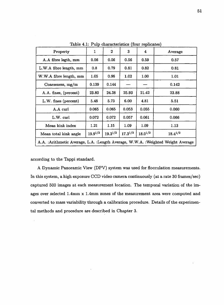
I A.A. :Arithmetic Average, L. A. :Length Average, W. W.A. :Weighted Weight Average I

according to the Tappi standard.

A Dynamic Panoramic View (DPV) system was used for flocculation measurements.

In this system, a high exposure CCD video camera continuously (at a rate 30 frames/sec)

captured 500 images a t each measurement location. The temporal variation of the im-

ages over selected 1.4mm x 1.4mm zones of the measurement area were computed and

converted to mass variability through a calibration procedure. Details of the experimen-

tal methods and procedure are described in Chapter 3.

TEST SECTION

Figure 4.3: Schematic diagram of the grid configuration and measuring area in the tur-

bulence rig test section, 50 cm downstream of the rig's inlet.

4.3 Results and Discussion

4.3.1 Flow Field Analysis

Different flow fields produced by the grids can be identified through a visual study of

a flowing pulp suspension using high-speed cinematography (Kerekes et al. 1985). In

this study a high exposure video camera with a speed of 30 frames/s was used to do a

similar analysis. The results of the present study was then combined with the results

of Kerekes et al. (1985) and the following conclusions were drawn. Figure 4.4 shows a

schematic diagram of the flow field near two grids located in the centre of the rig and

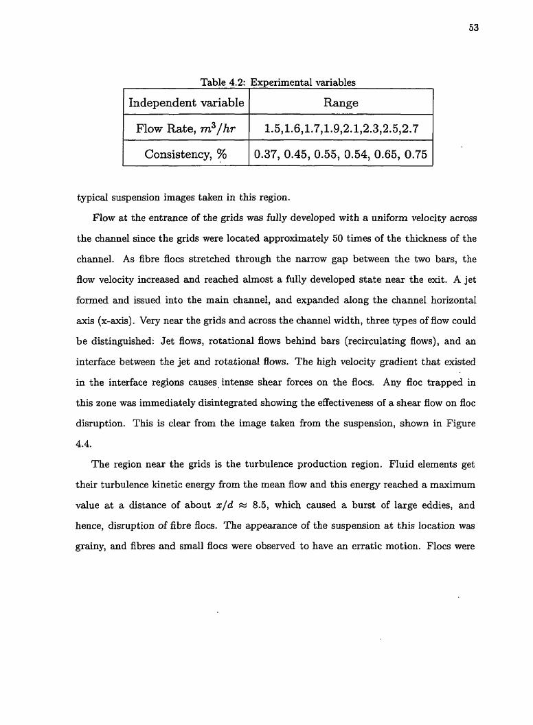
Table 4.2: Experimental variables

I Independent variable I Range

I Flow Rate, m3/hr 1 1.5,1.6,1.'7,1.9,2.1,2.3,2.5,2.7 1 I Consistency, % / 0.3'7, 0.45, 0.55, 0.54, 0.65, 0.75 1

typical suspension images taken in this region.

Flow at the entrance of the grids was fully developed with a uniform velocity across

the channel since the grids were located approximately 50 times of the thickness of the

channel. As fibre flocs stretched through the narrow gap between the two bars, the

flow velocity increased and reached almost a fully developed state near the exit. A jet

formed and issued into the main channel, and expanded along the channel horizontal

axis (x-axis). Very near the grids and across the channel width, three types of flow could

be distinguished: Jet flows, rotational flows behind bars (recirculating flows), and an

interface between the jet and rotational flows. The high velocity gradient that existed

in the interface regions causes intense shear forces on the flocs. Any floc trapped in

this zone was immediately disintegrated showing the effectiveness of a shear flow on floc

disruption. This is clear from the image taken from the suspension, shown in Figure

4.4.

The region near the grids is the turbulence production region. Fluid elements get

their turbulence kinetic energy from the mean flow and this energy reached a maximum

value a t a distance of about x/d x 8.5, which caused a burst of large eddies, and

hence, disruption of fibre flocs. The appearance of the suspension at this location was

grainy, and fibres and small flocs were observed to have an erratic motion. Flocs were

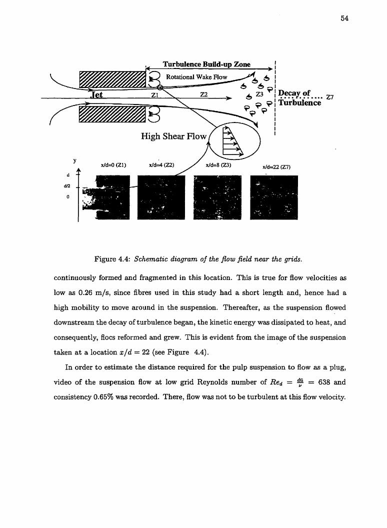
Figure 4.4: Schematic diagram of the flow field near the grids.

continuously formed and fragmented in this location. This is true for flow velocities as

low as 0.26 m/s, since fibres used in this study had a short length and, hence had a

high mobility to move around in the suspension. Thereafter, as the suspension flowed

downstream the decay of turbulence began, the kinetic energy was dissipated to heat, and

consequently, flocs reformed and grew. This is evident from the image of the suspension

taken a t a location x / d = 22 (see Figure 4.4).

In order t o estimate the distance required for the pulp suspension to flow as a plug,

video of the suspension flow a t low grid Reynolds number of Red = 5 = 638 and

consistency 0.65% was recorded. There, flow was not t o be turbulent at this Aow velocity.

It was observed that fibres accumulated behind the grids and flocs shed regularly into

the main stream. The jets issuing between the grids were straight near the grids and the

suspension was flocculated. As the jets expanded into the channel, a wavy flow pattern

propagated along the flow direction. The waves issued from different grids interact in

a very complicated way downstream of the grids. Near the grids, the suspension had

a very heterogeneous appearance but the homogeneity of the suspension increased over

the distance 0 < x ld < 10. At x/d x 10, large flocs were disrupted into smaller flocs and

smaller flocs collided with other Aocs to form larger flocs. The local shear stresses were

not strong enough to disperse fibre flocs into individual fibres and stable flocs grew until

the downstream position x / d sz 18, a t which point the suspension became a plug flow and

there was little or no relative movement of flocs and fibres. I t was then postulated that

the growth of stable flocs might correspond to the final decay of turbulence. Therefore,

as a rough estimate, the distance required for the pulp suspension to reach a highest

degree of flocculation a t a turbulent flow velocity 0.45mIs (Red = 3589) is x / d = 100.

In general, formation of Aocs in grid generated turbulence follows three stages: near

the grids, the turbulence production region, flocs are dispersed into individual fibres, this

region is followed by a transient region, where turbulence decays and transient flocs are

initially formed and then converted to stable flocs. Fibre flocs may join with others and

grow in size in this region to some extent. The final region is a region of pure growth

of stable flocs by a floc collision mechanism, which corresponds to the final decay of

turbulence. All flocculation measurements were carried in the transient flow region and

will be quantified in the sections which follow.

4.3.2 Longitudinal Flocculation Intensity

The evolution of the flocculation intensity (FZ) along the main flow direction at three

different lateral locations are shown in Figures 4.5 to 4.10.

Two regions downstream of the grid can be immediately identified. In the first

region, the flocculation intensity was high at the entrance of the jets issuing from the

gaps between the parallel bars, and in the wake of the bars. It decreased along the flow

axis and reached a minimum value at a distance of about x/d = 8.5. This region is

followed by the second region where the flocculation intensity increased along the flow

direction. The transition between these two regions, however, due to scatter in data,

is not sharply defined. The development of the streamwise turbulence and of the fibre

flocculation are strongly coupled. In the first region downstream of the grids there is

an intense production of turbulence due to the burst of the eddies, originated from the

flow field in the wakes, and due to the shearing action within the layers of the jet and

between the jet/wake '. In this region, fibre flocs are gradually dispersed as they move

downstream. This region extends from x/d=O to = 8.5 where the measured values for

the temporal mass variability or flocculation intensity (FZ) are decreasing.

'The grid generated turbulence may be inhibited by the channel wdl. Though wall turbulence has

different characteristics, one may argue that i t can be neglected in the centre plane of the rig and hence,

the grid generated turbulence may still keep its characteristics in the core of the channel. The effect of

top and bottom plates will be discussed in section 4.3.7.

0 10 20 30 40 x/d

Figure 4.5: Longitudinal ~occulatzon intensity at Ua = 0.45mlscc and C, = 0.54%

0 10 20 30 40 x/d

Figure 4.6: Longitudinal flocculation intensity at Ua = 0.45mlsec and C, = 0.5%

0 10 20 30 40

x/d Figure 4.7: Longitudinal jlocculation intensity at Ub = 0.26rn/sec and C, = 0.54%

Figure 4.8: Longitudinal jlocculation intensity at Ub = 0.26m/sec and C, = 0.42%

0 10 30 40 2%

Figure 4.9: Longitudinal flocculation intensity at Ub = 0.45mlsec and C, = 0.42%

0 10 30 40 3%

Figure 4.10: Longitudinal flocculation intensity at Ub = 0.26rnlsec and C, = 0.5%

In the present experiments the lowest flocculation intensity was achieved a t x/d w

8.5. In the second region (x/d > 8.5) turbulence began to decay and hence, the values

of Fl increased with x/d, which implies that the re-flocculation of fibres occurred at

a distance of about x/d = 8.5. After this distance, there was no significant difference

(an error of about f 5% as is typically shown in Figure 4.5 and all other figures having

a similar error bar) between Fl values observed in y-direction (at a given x/d). This

was confirmed by examining the F1 profiles at different x/d , and is presented in the

following section.

4.3.3 Flocculation intensity profiles

The flocculation intensity profiles normal to the streamwise direction, Figures 4.11 to

4.15, change from a parabolic shape between the grids, to a triple peak profile in the

wake region, and to a flat profile for downstream of the grids. The full data set is

given in Appendix A. Following the wake region there is a slow general increase in the

flocculation intensity. The suspension homogeneity was most a t x/dx8.5.

Figure 4.11: Flocculation intensity profiles at Ub = 0.45mlsec and C, = 0.54%

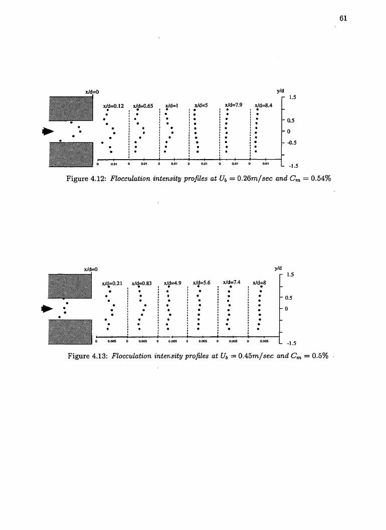
Figure 4.12: Flocculatzon zntensity profles a t Ub = 0.26mlsec and C, = 0.54%

Figure 4.13: Flocculatzon intensity profiles at Ub = 0.45mlsec and C, = 0.5%

Figure 4.14: Flocculation intensity proJiles at Ub = 0.26mlsec and C, = 0.5%

Figure 4.15: Flocculation intensity profiles at Ub = 0.45rnlsec and C, = 0.37%

Interface between two rotating flow cells. low flocculation intensity

! I / Centre of rotation,

A j / high flocculation intensity

! Core region of a jet , * -* .-..-..-..-..-..-..-.. +.- ..-..-..-..-........... * . . . . . . . . . . . -..-..-..-..-..- I high flocculation intensity 7

----/A --

! low flocculation intensity ! I

Jet and wake boundaries

Figure 4.16: Schematic diagram of the flow pattern near the exzt of two grids.

The Fl profiles within the channels between the two bars had a parabolic shape.

Flocculation was lowest near the wall regions, due to wall shear stress, and increased to

a maximum at the centre of the channel. Three lateral regions are identified a t the exit

of the bars: jet, wake, and jet/wake interface. The values of Fl in the bulk of the jet

flow was higher than that in the wake and interface between the wake and jet (y = d/2) .

Flow in the wake region is a rotational flow with a low velocity and increases toward the

jet axis, which could result in a high shear stress imposing on the surface of the flocs

trapped in this region. It can be seen that the measured values of F1 had a minimum

value in this region. Interestingly, the flocculation profiles show that Fl increases in the

upward direction reaching a maximum value a t a distance about a quarter of the bar

width ( y = 3d/4). It then decreased to a minimum value in the middle of the bar ( y = d) .

The corresponding flow pattern is illustrated in Figure 4.16. This type of behavior may

be explained by considering that the flow behind a bar includes two counter rotating

flow cells each having a height approximately equal to the half of the width of a bar. In a

rotational field, fibres rotate integrally until they shed into the main stream. This type of

rotational shear flow would enhance flocculation (see Kao and Mason 1975). However, a t

the interface between the two rotating cells, flocculation, due to extension, was found to

be lower than that in the core region. Due to the complexity of the turbulence structure

in the immediate wake of the bars, the effects of the mean concentration and velocity

on the location of the centre of the rotation, where FI is locally maximum, are complex.

However, the results indicate that a decrease in the mean flow velocity shifts forward

the centre of rotation of the flow cells (see Figure 4.16).

4.3.4 Homogeneity

The homogeneity of the pulp suspension across the channel at different downstream

locations was defined as the standard deviation of FI profiles. The result is shown

in Figure 4.17. The standard deviation near the grids has a large value and decreases

exponentially with x/d, which implies the suspension homogeneity increases in the down-

stream direction. This is coincident with the increase in the axial dispersion along the

flow direction as a result of the interactions between wakes and jets, and the burst of

eddies. The homogeneity near the grids was increased with both flow velocity and bulk

concentration. These effects are discussed in the next two sections.

4.3.5 Effect of flow velocity

The typical effect of the bulk velocity on the flocculation intensity is shown in Figure

4.18. An increase in the flow velocity resulted in a decrease in the flocculation intensity,

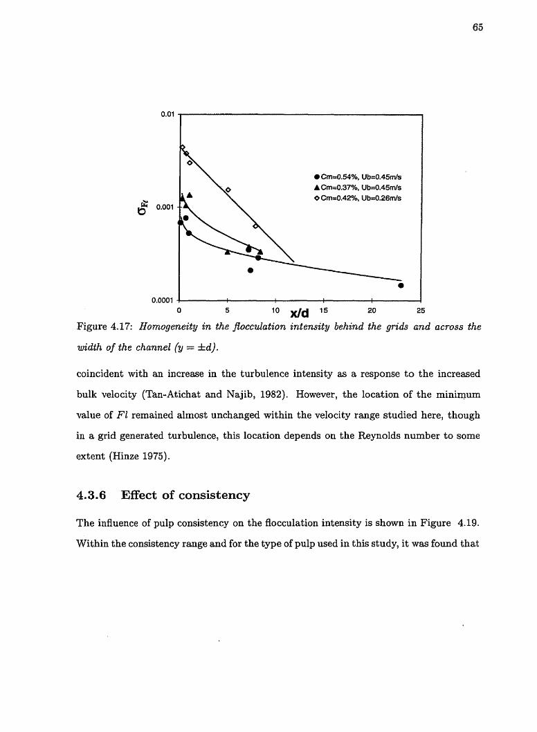
0 5 10 x/d 15 20 25

Figure 4.17: Homogeneity in the _flocculation intensity behind the grids and across the

width of the channel (y = &dl .

coincident with an increase in the turbulence intensity as a response t o the increased

bulk velocity (Tan-Atichat and Najib, 1982). However, the location of the minimum

value of Fl remained almost unchanged within the velocity range studied here, though

in a grid generated turbulence, this location depends on the Reynolds number to some

extent (Hinze 1975).

4.3.6 Effect of consistency

The influence of pulp consistency on the flocculation intensity is shown in Figure 4.19.

Within the consistency range and for the type of pulp used in this study, it was found that

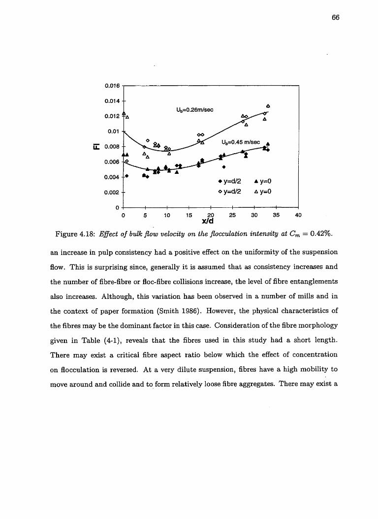
F i g I: Effect of bulk POW velocity o n the flocculation intensi ty at C, = 0.42%.

an increase in pulp consistency had a positive effect on the uniformity of the suspension

flow. This is surprising since, generally i t is assumed that as consistency increases and

the number of fibre-fibre or floc-fibre collisions increase, the level of fibre entanglements

also increases. Although, this variation has been observed in a number of mills and in

the context of paper formation (Smith 1986). However, the physical characteristics of

the fibres may be the dominant factor in this case. Consideration of the fibre morphology

given in Table (41 ) , reveals that the fibres used in this study had a short length.

There may exist a critical fibre aspect ratio below which the effect of concentration

on flocculation is reversed. At a very dilute suspension, fibres have a high mobility to

move around and collide and to form relatively loose fibre aggregates. There may exist a

critical concentration below which flocculation could increase with concentration (Ritala

and Huiku 1989). Above this concentration and within the range studied here, short

fibres have a high mobility to move around and fill out the pore structure of loose flocs

and fibre network without being entangled with the other fibres. Adding more of these

short fibres by increasing concentration smooth out the mass non-uniformity and hence

reduces fibre flocculation. It is worth mentioning that the effect of concentration on

the flocculation intensity even when mass variability data presented in a non-normalized

form, i.e. absolute values, did not change.

Figure 4.19: Eflect of pulp consistency on the jlocculation intensity at Ub = 0.45mlsec

4.3.7 Characterizing flocculation

In the decaying period of grid generated turbulence of a single phase fluid in wind or

water tunnels, where turbulence is homogenous and nearly isotropic, i t is known that

the streamwise turbulence intensity decays as Tu ( ~ c / d ) - ~ (Gad-El-Hak and Corrsin

1974, Roach 1986, Mohamed and LaRue 1990 ) . Different types of grids and flow

modifiers used in wind tunnels (Roach 1986, Oshinowo 1997) confirms the universality

of the exponent n as 5/7, in agreement with the theoretical analysis of Kolmogorof.

Effect of wall turbulence

Laser Doppler Anemometry (LDA) techniques have been used to measure the turbulence

intensity of a pulp suspension flowing through a turbulence rig (Kerekes and Garner 1982,

d'Incau 1983), a flow channel similar to that used in this work. Figure 4.20 shows the

comparison between these measurements and the decay power law. Within the accuracy

to which the experimental data was re-plotted, agreement appears to be satisfactory.

Although the formation and growth of eddies are influenced by the upper and lower

channel walls in a single phase flow (Roach 1986), the turbulence decay law remained

unchanged. Best agreement is expected for x/d > 8.5, i.e. in the decaying turbulence

region.

In the range x / d FZ 7 - 8.5 the turbulence generated by the grids are dominant

over the wall generated turbulence. As turbulence decays, the wall effects become more

important but a t the same time fibre flocs become more structured as well. The latter

process is very fast and in effect it results in a transient state of flocculation. Fibre flocs

could be dispersed due to the existence of high shear forces in the region very near the

8 0 Water

Pulp (0.45%)

Figure 4.20: Comparison between the measured turbulence intensi ty and power law model

of the decay of turbulence (data from d'lncau (1983)).

wall. But, it appears that these forces contribute little to floc disruption in the central

region within the parametric range studied since the flocculation intensity continues t o

increase. In summary, the results suggest that the measured values of the flocculation

intensity are only marginally lower due to wall shear than results that would be expected

for a purely grid generated turbulence flow field.

Clearly the present results indicate that the decay of turbulence promotes floccula-

tion. In all experimental data shown through Figures 4.5 to 4.10, after a certain distance

from the trailing edge of the grids, the flocculation intensity monotonically increased

with x/d. In other words, the flocculation is inversely proportional to the turbulence

intensity.

Let us postulate that the flocculation intensity downstream of a grid may be expressed

as a function of the grid geometry (possibly through its solidity and/or coefficient of

static pressure drop), the streamwise distance from the grid, the flow Reynolds number,

and physical characteristics of the fibres . In the present work, only one type of grid and

pulp were used. Therefore, i t is expected that the fiocculation intensity can be expressed

solely as a function of Reynolds number (Re = %), consistency, and z / d as

Bulk quantities

The consistency term, CA, must be included as a separate term in Equation (4.1), al-

though one may argue that the effect of consistency has already been associated with

the definition of Reynolds number through the dynamic viscosity of the medium. An

increase in consistency results in an increase in viscosity, and the removal of the consis-

tency term wouId require a negative exponential value for a to be consistent with the

results presented in section 4.3.6. Flocculation would then always have to be a decreas-

ing function of consistency, which is not necessarily the case2. Therefore, the Reynolds - - - --- -

21n fact if we assume v - ~ b : , where b' is a wood fibre character (hardwood or softwood) and v is

viscosity then, it follows that F1 - Ca$. Now, experiments show that a < 0 and hence, -ab' > 0.

This means that increasing consistency will always enhance flocculation, which has not always been

observed to be the case. A separate consistency term is therefore necessary.

number is simply defined for water, i.e. Re, = a uw and consistency effects are treated

separately.

Equation (4.1) implies that at constant x/d, the effect of consistency, C,, and bulk

velocity may be characterized through following equation:

To test the adequacy of Equation (4.2), flocculation measurements were carried out

a t a constant location far downstream of the grids in the experimental turbulence decay

region of the flow at x/d = 27. The Reynolds number and pulp consistency studied were

in the range 2000 c Re, < 3600 and 0.45 < C, < 0.75. The effect of bulk flow velocity

at different consistencies is shown in Figure 4.21, This figure shows that the flocculation

intensity increased as the pulp consistency decreased and decreased with an increase in

the flow velocity.

Fitting Equation (4.2) to the data yields the following relationship:

The coefficient of the correlation, r2, is 0.96. Shown in Figure 4.22, Figure 4.21 is

re-plotted using the above relationship.

Rate of Growth

According to Equation (4.1), a plot of Fl versus x/d in a log-log plot a t a given con-

sistency and bulk velocity, should yield a straight line with a slope m. The validity of

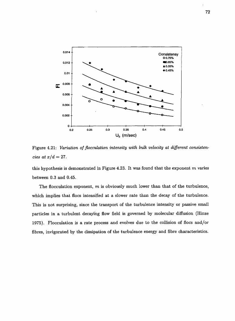
Consistensy 0 0.75%

0.65% A 0.55% + 0.45%

Figure 4.2 1: Variation of flocculation intensity with bulk velocity at di;gkrent consisten-

cies at x/d = 27.

this hypothesis is demonstrated in Figure 4.23. It was found that the exponent m varies

between 0.3 and 0.45.

The flocculation exponent, rn is obviously much lower than that of the turbulence,

which implies that flocs intensified at a slower rate than the decay of the turbulence.

This is not surprising, since the transport of the turbulence intensity or passive small

particles in a turbulent decaying flow field is governed by molecular diffusion (Hinze

1975). Flocculation is a rate process and evolves due to the collision of flocs and/or

fibres, invigorated by the dissipation of the turbulence energy and fibre characteristics.

Figure 4.22: The correlation between flocculation intensity and Reynolds number and

mean consistency with r2 = 0.96 at x/d = 27.

Self-preservation relationship

Returning to Equation (4.1), a statistically more significant value for the exponent m

may be obtained if the data, plotted through Figures 4.5 to 4.10, were re-plotted using

exponents in the relationship (4.3). This is demonstrated through Figure 4.24. Appar-

ently all 200 experimental data used in this figure, collapsed onto a single line with a

slope 3.197. Therefore, the following self-preservation relationship for the pulp used in

this study is proposed:

Figure 4.23: Comparison between the empirical power law and j3occulation interisity

downstream of the grid at Ub = 0 . 4 5 1 ~ ~ 1 ~ .

4.4 Closure

A unique experimental study for the purpose of identifying parameters affecting fibre

flocculation in a decaying turbulence field was carried out. A dynamic panoramic view

technique was used to measure the flocculation intensity of a kraft hardwood pulp behind

a grid generated turbulence flow field. Based on this study, the following findings and

conclusions are drawn:

1. Longitudinal flocculation intensity data were obtained. They revealed the existence

of two distinct regions behind the grids. Near the grids, flocculation along the axis

of jets and wakes decreased to a minimum vaIue at x /d = 8.5. Further downstream

of the grids, the flocculation intensity monotonically increased with x/d.

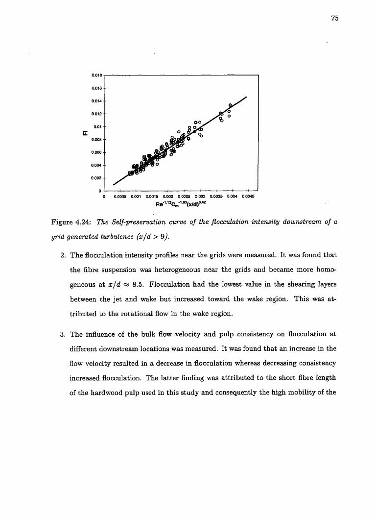
Figure 4.24: The Self-preservation curve of the fEocculation intensity downstream of a

grid generated turbulence (x/d > 9).

2. The flocculation intensity profiles near the grids were measured. It was found that

the fibre suspension was heterogeneous near the grids and became more homo-

geneous at x / d = 8.5. FloccuIation had the lowest value in the shearing layers

between the jet and wake but increased toward the wake region. This was at-

tributed to the rotational flow in the wake region.

3. The influence of the bulk flow velocity and pulp consistency on flocculation at

different downstream locations was measured. It was found that an increase in the

flow velocity resulted in a decrease in flocculation whereas decreasing consistency

increased flocculation. The latter finding was attributed to the short fibre length

of the hardwood pulp used in this study and consequently the high mobility of the

fibres; for longer fibres, an increase of flocculation with consistency is normal in

low shear fields.

4. Using the analogy between turbulence and flocculation, the flocculation intensity

of the pulp fibres used in this study was characterized through effects of bulk

quantities and non-dimensional distance, x / d .

5. Flocculation was found not to follow the inverse of the decay of turbulence. The

decay of turbulence (TU-' - ( ~ / d ) ' . ~ ) was found to be faster than the growth of

flocs (Fl - ( ~ / d ) ' - ~ ~ ) .

6. Flocculation growth exhibited a self-preservation behavior for 200 data points ob-

tained at different velocities and consistencies.

Chapter 5

Characteristics of Fibre Floes in

Turbulent Flows

5.1 Introduction

The local mass variability or flocculation intensity necessarily is a useful measure of uni-

formity of a flowing pulp suspension. The other complementary factor which determines

the scale of mass uniformity is the floc size distribution. The latter has been described

by many researchers in different ways. Persinger and Mayer (1975) defined the scale of

flocculation analogous to the turbulence statistics as being the result of averaging the

correlation between local concentrations at different times (autocorrelation function).

In some cases (see Nerelius et al. 1975, Bonano 1984) the frequency analysis technique

has been used to characterize floc sizes. In this technique, the time domain of fluctuating

concentration is converted to the frequency domain (See section Chapter 2). The scale

of flocs can then be defined with respect to the mean flow velocity at a given frequency.

Image analysis techniques may also be used to obtain floc size distributions. Kaji et.al.

(1991) converted the image to fibre flocs in a flowing suspension to a binary image from,

define boundaries for flocs and hence, determine the area of flocs.

The differences in defining fibre flocs, mentioned above, may result in different values

for the floc size. The origin of this inconsistency is due to the irregular shape of flocs

and the fuzzy boundary of flocs. An objective of this work is to introduce a unique

definition for the structure of fibre flocs. Hitherto, no model has been proposed to define

the internal structure of flocs in suspensions or in paper. Using the mass-action law,

Hourani (1988) proposed a theoretical floc size distribution. This distribution function

has two unknown parameters, both must be estimated from experimental data.

There is no non-intrusive technique to measure the floc size distributions in the plane

normal to the flow direction l . Here, an analytical approach will be taken to propose

a novel statistical geometric model t o define the internal structure of flocs, namely, a

random walk of free-fibre-lengths. This will lead to a transverse floc size distribution

(FSD) function. It is shown that this distribution function has three parameters, which

jointly represent the state of flocculation. Two of these parameters have already been

used by Dodson and Sampson (1996) to represent the distribution of pores in paper.

I t is shown that for a given fibre/fibre gap size distribution, the FSD function predicts

the corresponding floc size distribution. Using pore size distribution data for hand-

sheets, obtained by the flow permeability technique, estimates of the FSD parameters

and corresponding floc size distributions will be estimated.

lIn fibre suspension flows, the scale of flocculation should be considered in both longitudinal and

transversal directions. The former measures the scale of non-uniformity in the paper machine direction

(MD) whereas the latter is a measure of non-uniformity in a plane perpendicular to the flow direction.

I t will be shown that the results of the statistical geometric model are in excellent

agreement with the classical relative diffusion theory (Richardson 1926) as its particular

case. This is an extremely important property of this model. Since, while the direct mea-

surement of transverse-plane scale of flocculation is extremely difficult, measurements

of the relative diffusing particles seem to be more practical. Last but not least, it will

be shown that the model can also describe the longitudinal/Eulerian type of floc size

distributions. This model will be compared with Hourani's experimental data (Hourani

1988).

5.2 Transverse floc size distributions

The transverse distribution of fibres in a flowing pulp suspension is presumably closely

connected to the transport of eddies at different length scales. Both experimental ev-

idence and theoretical analysis indicate that the transverse paths of these eddies in a

one-phase isotropic and homogeneous turbulent flow field can be modeled by an ordinary

random walk process (Hinze, 1975). The Gaussian distribution function which results

from this model is also a solution to the diffusion equation with a constant coefficient of

eddy diffusivity. This implies that the lateral spread of the fluid lumps follows a diffu-

sion mechanism. According to Hinze (1975), the size of those fluid lumps contributing

to this diffusion transport mechanism has the same order of magnitude as the larger

eddies; namely, an integral length scale of turbulence for long diffusion times. But for

short diffusion times, all eddies contribute to this transport.

In fibre suspension flows, the local turbulence length scale is influenced by the pres-

ence of fibres (Kerekes 1982, Steen 1990). Using a LDA technique, Steen (1989) measured

turbulence spectra of a flowing fibre suspension a t various positions downstream of a dif-

fuser. At a relatively low Reynolds number, he reported higher turbulent energy almost

a t lower turbulence length scale due to presence of fibres in the fluid. Although the peak

of energy distributions occurred at a scale of about the diffuser height (2 mm), elevated

energy level could still be observed a t lower scales down to 0.6 mm. Steen suggested that

fibre flocs force the turbulent eddies to be present in fluid layers between the flocs. He

did not, however, comment on the generation of turbulence due to the solid boundaries

of fibres inside of flocs. If there were a relative velocity between fibres inside of the

Aocs and surrounding fluid, additional turbulence energy might be produced inside of

the flocs. If i t is assumed that the local network of fibres acts like a deforming screen

(or grid) mounted perpendicular to the main flow direction and has a relative velocity

with respect t o the surrounding fluid. Then, the relevant local length scale may be

characterized by the mesh or pore size of the fibre network. The size of such pores, of

course, varies with time and location in an erratic fashion, which, unfortunately, under-

mines the possibility of a deterministic model. Moreover, due to the flow discontinuity

a t the boundaries of fibres, writing a diffusion equation for the marked fluid particles

with a constant coefficient of eddy diffusion must fail. This will be discussed latter in

section 5..2.5. As a simplification, represent the flow of a fibre as flow over a cylinder.

The coefficient of eddy diffusion varies with distance and is maximum in the core of the

wake flow (mixing zone) and decreases in downstream direction, where the flow is less

turbulent.

In a statistical geometric approach, which will be presented in the next section, a

stochastic local fibre network (clump) of a given pore (eddy) size is first defined. This

approach resembles the equivalent process of turbulent diffusion in an isotropic and

homogeneous turbulence at a given eddy (pore) size length scale. Then, the contribution

of the variability in the turbulence length scale (pore size distribution) is taken into

account by superpositioning an infinite number of such clumps, each having a different

pore size.

5.2.1 Stochastic Fibre Clumps

Consider the structure of a local fibre clump, or 'floc', as a chain of random fibre segments

that can be generated by the path of a random walk process. In this process the walker

starts from some origin and steps a length equal to the fibre-fibre gap length to reach

a contact point which defines an adjacent intersection with a fibre. The walker may

then change direction for the next step to reach a new contact point, and continue for

N steps. The sequence of individual steps F = (C,G, 6, . . . ,%) gives a representative

structure for a path through a clump, along free fibre segments. We define the distance

r = 16 + F2 + F3 + ... + FN [ t o be the clump size. Then r has a probability density function

P(r lg), parameterized by the gap length g > 0 and is known (Weiss 1994) to have the

form

This procedure for constructing a local fibre clump is essentially the standard random

walk proposed by Rayleigh (1919). Random walks will be used to represent a range

of fibre clumps, each with constant gap length, the gap lengths being drawn from a

population with probability density function of gamma type:

with k, 6 > 0. This model is justified since clumps arise in the fibre fluidization from

turbulent diffusion; locally there is a characteristic length scale and we adopt this as

a gap length for the locality. So, essentially, a gamma distribution is ascribed to the

variability of turbulence length scale in the fluidized fibre suspension and the proposed

local random walks are representative of the cores of fibre clumps.

The case k = 1 reduces the gamma distribution to the exponential distribution, and

may be viewed as representing the true random case-when fibres are placed indepen-

dently, then any path through the network is a realization of a 1-dimensional Poisson

process (Deng and Dodson 1994). Departures from the random state are parametrized in

terms of the two positive real numbers k and 6. This approach was also used in (Dodson

and Sampson 1996) to model porosity in stochastic fibrous networks. The probability

density function for clumps of size r, averaged over all possible gap lengths is

Introducing dimensionless variables X = 6 r / O and Z

function for X is:

= bg , the probability density

Though there is apparently no analytical expression for the integral in (5.4)) the

moments of this distribution function can be evaluated analytically, as will be shown

in the next section, by changing the order of integration. Note that the distribution

function (5.4) is automatically normalized

Integrals of the type in (5.4) have attracted the attention of approximation theorists,

who have built on the earlier work of Laplace. The present analysis makes use of an

asymptotic approximation originally given by Erdelyi (1961). The form of the solution

used here is discussed in detail by Wong (1989) as Example 2 in pages 62-66 and takes

the fbrm

which can be compared numerically with the exact expression. Note that (5.6) is not yet

normalized because i t does not exactly satisfy (5.5). Figure (5.la) shows the variation

of the error with the k parameter, which turns out t o be less than 10% in the range

0.6 < k < 2.8. This error is reduced further by renormalizing (5 .6 ) , Figure (5.lb), as

follows

2 k -1 3x213 where A = J ~ x * E ~ ( - ~ ) ~ x .

The error associated with the mean of the distribution (5.7) is less than 10% for

the range 0.5 < k < 3, which turns out to cover the range of interest from the work of

Dodson and Sampson (1996). In the next two sections, some of the properties of (5.4)

are investigated and a method for estimating the parameters k , N, and 8 is proposed.

Typical plots of equation (5.7) for the values 12=0.5, 1, 2, and 3 in Figure 5.2 indicate

Error, %

Figure 5.1: a) (left) Variation of the error associated with approximation (5.6) and b)

(right) with that of approxzmation (5.7) relative to the true value (5.4).

that, as k increases, the shape of the resulting distribution function shifts from a negative

exponential type to a log-normal shape.

5 2 . 2 Variability

As mentioned above, the moments of the distribution function (5.4) may be determined

analytically and it turns out that there is a power law relationship between its mean

0 1 2 3 4 5

x Figure 5.2: The shape of the self-similarity distribution function (5.7) shifts from a

negative exponential function to a log-normal type as the intrinsic fiocculation parameter,

k , increases.

and standard deviation. The qth moment of the distribution function, P ( X ) , is

Introducing P ( X ) from (5-4) into (5-8), we get

where 33 = (3) (&/a)'. The moments of the distribution (5.7) with (5.9) are compared to estimate the relative

error of using our approximation. Figure 5.1 (right) shows the variation of this error

with the parameter % for the first five moments of the floc size distribution. These errors

are acceptable for practical paper manufacturing purposes.

The mean and standard deviation of P(X) are given by:

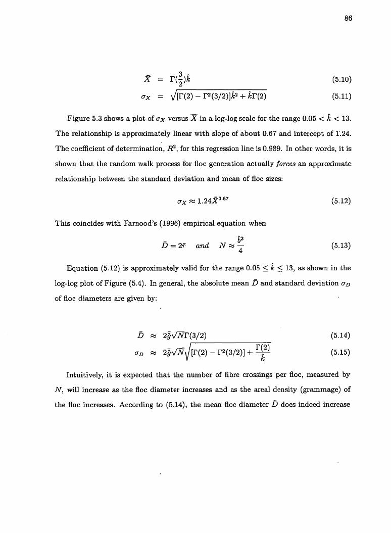
Figure 5.3 shows a plot of versus X in a log-log scale for the range 0.05 < k < 13.

The relationship is approximately linear with slope of about 0.67 and intercept of 1'.24.

The coefficient of determination, R2, for this regression line is 0.989. In other words, i t is

shown that the random walk process for floc generation actually forces an approximate

relationship between the standard deviation and mean of floc sizes:

This coincides with Farnood's (1996) empirical equation when

i2 D = 27 and N c - 4

Equation (5.12) is approximately valid for the range 0.05 5 i 5 13, as shown in the

log-log plot of Figure (5.4). In general, the absolute mean b and standard deviation

of floc diameters are given by:

Intuitively, it is expected that the number of fibre crossings per floc, measured by

N , will increase as the floc diameter increases and as the areal density (grammage) of

the floc increases. According to (5.14), the mean floc diameter D does indeed increase

Figure 5.3: T h e relationship between the dimensionless standard deviation a, and the

mean offEoc size, on a log-log plot. T h e dot points are calculated from equations (5.9)

and (5.10) and the solid line is. the best linear regression fit to these points, which has a

slope of 0.67.

with increase in N. However, when more fibre segments are involved in a floc, it may

be expected that the mean gap length 5 will decrease. Presumably, there is likely to be

a lower bound on the mean gap by packing constraints on fibres being jammed in. So,

to have 5, increasing because more fibres are present, 8 must not decrease as quickly as

37 The process of constructing the fibre clumps, described above, is analogous to the

diffusion process, since the diffusion path is necessarily equivalent to the random walk

process. If the fibrous structure of paper is similar to that in a suspension, the model

suggests that the lateral flow through a sheet of paper may also be described by the

diffusion model as well. This similarity hypothesis will be used to evaluate the model's

predictions from experiments performed on paper. The structural analyses, however,

differ when it comes to the superposition of flocs. For example, it is known that com-

mercial papers usually have a stratified structure for hydrodynamic filtration reasons

and that there is usually a negative local vertical correlation between strata (Deng and

Dodson 1994). In paper, a superposition of similar flocs does not completely describe the

varying drainage conditions during paper forming. In the section which follows, the ex-

perimental data on paper will be fed to the proposed model to examine how realistically

this model can predict a floc size distribution from a given pore size distribution.

5.2.3 Floc size estimates from fluid permeation

Here, we study the possibility of estimating an apparent floc size distribution from a fluid

permeation technique performed on a sheet of paper. Pore size distributions in paper

can be obtained by different techniques. For example, a gas-drive technique (Bliesner

1964) involves with stepwise penetration of a gas through the sample above which there

is a column of liquid. The pressure beneath the sample is increased slowly until the first

bubble is observed in the liquid. The hydraulic pore radius, opened to flow at a pressure

drop AP, is then obtained from r, = &, where 7 is the surface tension of the wetting

liquid.

Dodson and Sampson (1996) used some of the experimental data in (Corte and

Lloyd 1965) to quantify effects of flocculation on the pore size distribution. According

t o Dodson and Sampson (1996), the pore size distributions can be characterized by

the two parameters k and b, of a gamma distribution, (5.2). They are given in Table

(5.1). Here, their method is extended t o interpret the effect of sheet density on the pore

size distribution. For this purpose we use experimental data given in (Corte and Lloyd

1965). Figure 5.4 compares the model equations (6 to 8) developed in (Dodson and

Sampson 1996) with the log-normal plots of experimental data. The full data set with

the corresponding k and b is given in Table (5.2).

Frequency Frequency

Figure 5.4: Effect of sheet density o n pore size distribution. Broken line is the log-

linear plot of the experimental data (Corte and Lloyd, 1965) for softwood (lef41 and

hardwood (right) sulfate pulp. Solid line represents the model equation (6) in (Dodson

and Sampson, 1996).

On the assumption that the gap size distribution in (Dodson and Sampson 1996)

coincides with that in our flocs, k = A, b = 5, and tj = i . An average value for N is

estimated as the product of the ratio of mean fibre length, A, to mean gap length g,

times the expected number of fibres in a spherical volume of diameter one mean fibre

length, n,,,d, (Dodson 1997). X

N = 5%,d 9

Now (5.14) and (5.15) are used to determine the corresponding mean and standard

deviation of floc sizes, given in Tables (5.1) and (5.2). In the case when a sheet of paper

is formed from couched layers, N should be multiplied by the number of layers.

Table 5.1: Parameters of the pore and apparent floc size distributions- Effect of floccu-

Sample type and ~ i f e r e n c e - I Ai;m

sw-layerd structure [CL]

sw-light flocculation [CL]

sw-medium Rocculation [CL]

lation

sw-Iteavy flocculation [CL] 1 2.2

Data from (Dodaon and Sampaon, 1996)

hw-layered structure (CL1 1 0.68

Estimated parameters

in this study

--

I hw-heavv flocculation lCLl 1 0.68 1 24.7 1 0.02982 1 1.03 1 36 I 13.3 I 1.254 I 1 . 4 1 1 503 1 --

~ ~ = s o f t wood; hw=hard wood

[CLkCorte and Lloyd. 1965

Figure 5.5 reveals the relationship between the mean and the standard deviation

of floc sizes a t a constant sheet density in a log-log plot. From this figure it is clear

that all data points lie on a straight line with a slope of about one. Even changing the

sheet density while keeping the crowding number constant does not have a substantial

effect on this relationship, as shown in Figure 5.6 (right). As seen in Figure 5.5, .the

theoretical predictions are in fair agreement with the regression equation proposed by

Table 5.2: Parameters of the pore and apparent floc size distributions- Effect of sheet

density Sample type and Reference Density, % n,,,,d g k b[mm-l] r>[p] b[mm]

sw [CL] 0.235 0.2 0.04714 1.334 28.30 22.12 0.2563

sw [CL] 0.422 0.2 0.02170 1.545 71.20 10.46 0.1732

sw [CL] 0.683 0.2 0.01360 1.643 121.7 6.660 0.1366

sw [CL] 0.690 , 0.2 0.00968 1.815 189.4 4.720 0.1161

1 [CL]=Corte and Lloyd, lg6S I

-

Irw [CL]

hw [CL]

hw [CL]

(Farnoodl 995).

The relationship between the mean pore size, determined from a laminar flow perme-

sw=soft wood; hw=hard woad

-

0.664

0.636

0.706

ation technique, and calculated mean floc size is shown in Figure 5.6. The mean floc size

increases monotonically as the mean pore size increases. In a log-log plot, the relation-

-- -

0.1

0.1

0.2

ship is linear when the handsheets had different densities while made from suspensions

of constant crowding number.

0.00744

0.00563

0.00497

Using the data from Table (5.2), an estimate of the effect of sheet density on the

mean floc size is obtained as shown in Figure 5.7. Apparently, the effective mean

floc size decreases as the sheet density increases. This means that more uniformity is

expected by increasing sheet density, in agreement with observation (Bliesner 1964).

Waterhouse (1992) showed that wet pressing not only increases the apparent density of

paper but also reduces the net coefficient of variation of local grammage. So material is

redistributed laterally in the sheet, presumably by the smoothing of thicker regions to

fill thinner regions. As was expected, Figure 5.7 also shows that the predicted mean

2.139

1.814

2.410

287.4

322.5

485.0

3.740

2.770

2.530

0.0399

0.0347

0.0326

0.0372 9.137

0.0342

0.0292

12.089

13.685

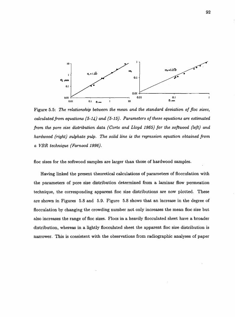
0.01 0.1 6.- I 10 D.nm

Figure 5.5: The relationship between the mean and the standard deviation of fEoc sizes,

calculated from equations (5-14) and (5-1 5). Parameters of these equatzons are estimated

from the pore size distribution data (Corte and Lloyd 1965) for the softwood (left) and

hardwood (right) sulphate pulp. The solid line is the regression equation obtained from

a VBR technique (Farnood 1996).

floc sizes for the softwood samples are larger than those of hardwood samples.

Having linked the present theoretical calculations of parameters of flocculation with

the parameters of pore size distribution determined from a laminar flow permeation

technique, the corresponding apparent floc size distributions are now plotted. These

are shown in Figures 5.8 and 5.9. Figure 5.8 shows that an increase in the degree of

flocculation by changing the crowding number not only increases the mean floc size but

also increases the range of floc sizes. Flocs in a heavily flocculated sheet have a broader

distribution, whereas in a lightly flocculated sheet the apparent floc size distribution is

narrower. This is consistent with the observations from radiographic analyses of paper

Menn Pore Size. pm

Figure 5.6: The relationship between the calculated mean floe size (equation (5.14)) and

10 7

measured mean pore size.

B d. .- VJ 1 : 8 . : E 8

(Farnood and Dodson 1995). Figure 5.9 shows the effect of sheet density on the apparent

floc size distribution for sulphate pulp. Flocs have a broader distribution at lower sheet

density and, on average, they are larger in size.

' .SW(Effectof 0 Sheet density)

A HW (Effect of Sheet Density) 2 o S W ( E f k t of flocculation)

5.2.4 Comparison with the relative turbulent diffusion theory

/n HW (Effect of flocculation)

Richardson (1926) was the first who studied the relative diffusion of a pair of particles

located within the lumps of a turbulent flow field. The importance of the relative diffu-

sion becomes evident when one realizes that the motion of a single particle is dominated

by the energy containing eddies (see e.g. Hentschel and Procaccia 1984, Hinze 1975),

whereas the relative motion of a pair of particles is dominated by eddies of smaller size,

in the order of magnitude of the interparticle distances. Analogous to the Richardson

theory, consider the relative diffusion of couple particles, initially released a t a close

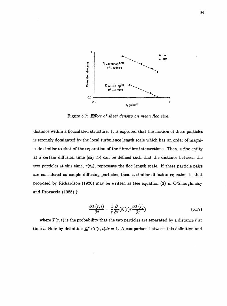
Figure 5.7: E$ect of sheet density o n mean floc size.

distance within a flocculated structure. It is expected that the motion of these particles

is strongly dominated by the local turbulence length scale which has an order of magni-

tude similar to that of the separation of the fibre-fibre intersections. Then, a, floc entity

a t a certain diffusion time (say td) can be defined such that the distance between the

two particles at this time, ~ ( t ~ ) , represents the floc length scale. If these particle pairs

are considered as couple diffusing particles, then, a similar diffusion equation to that

proposed by Richardson (1926) may be written as (see equation (3) in O'Shaughnessy

and Procaccia (1985) ):

where T(r , t ) is the probability that the two particles are separated by a distance Fa t

time t. Note by definition rT(r, t ) d r = 1. A comparison between this definition and

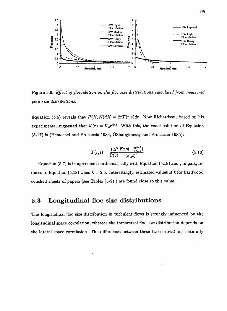
-.-.-- HW Light Rocculntion - HW Hcnvy Rocculntion

4 - ....... , SW Light

3.5 -. - - SW Medium

7'

o 2 0 0 e 5 floe size, mm 1 1.5 2

Figure 5.8: Eflect of flocculation on the floc size distributions calculated from measured

pore size distributions.

Equation (5.5) reveals that P ( X , N ) d X = 2rT(r, t)dr. Now Richardson, based on his

experiments, suggested that K(r) = ~ , r ~ / ~ . With this, the exact solution of Equation

(5-17) is (Hentschel and Procaccia 1984, Oshaughnessy and Procaccia 1985):

Equation (5.7) is in agreement mathematically with Equation (5.18) and , in part, re-

duces to Equation (5.18) when % = 2.5. Interestingly, estimated values of % for hardwood

couched sheets of papers (see Tables (5-2) ) are found close to this value.

5.3 Longitudinal floc size distributions

The longitudinal floc size distribution in turbulent flows is strongly influenced by the

longitudinal space correlation, whereas the transversal floc size distribution depends on

the lateral space correlation. The differences between these two correlations naturally

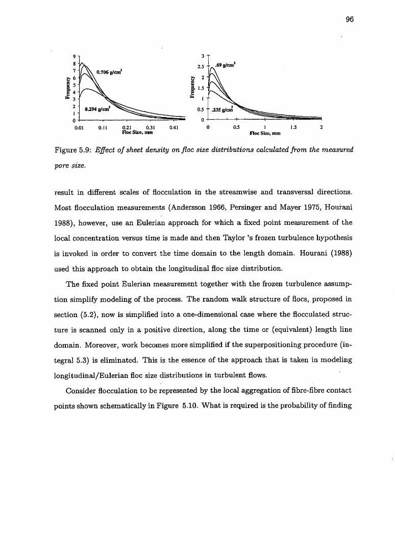
0.01 0.1 1 0.21 0.31 0.41 0 0.5 I 1.5 2 Floc Size, mm Floc Size, mm

Figure 5.9: Effect of sheet density on ftoc size distributions calculated from the measured

pore size.

result in different scales of flocculation in the streamwise and transversal directions.

Most flocculation measurements (Anderson 1966, Persinger and Mayer 1975, Houiani

1988), however, use an Eulerian approach for which a fixed point measurement of the

local concentration versus time is made and then Taylor 's frozen turbulence hypothesis

is invoked in order to convert the time domain to the length domain. Hourani (1988)

used this approach to obtain the longitudinal floc size distribution.

The fixed point Eulerian measurement together with the frozen turbulence assump-

tion simplify modeling of the process. The random walk structure of flocs, proposed in

section (5.2), now is simplified into a one-dimensional case where the flocculated struc-

ture is scanned only in a positive direction, along the time or (equivalent) length line

domain. Moreover, work becomes more simplified if the superpositioning procedure (in-

tegral 5.3) is eliminated. This is the essence of the approach that is taken in modeling

longitudinal/Eulerian floc size distributions in turbulent flows.

Consider flocculation to be represented by the local aggregation of fi bre-fibre contact

points shown schematically in Figure 5.10. What is required is the probability of finding

the nth contact point on a fibre somewhere in the interval (x, x+dx), where x is the

distance from one end of the fibre. Since x = C xi, the sum of the individual gaps, the

required probability density function &(x) will depend upon the individual distribution

functions , 4 ( x i ) 's, associated with the gap lengths, xi. Assuming that all these xi's are

independent and that the ~ ( x ~ ) ' s are identical, it can be shown

l o o %(z) = , Im P (w) e-iwxdw (5.19)

where &w), the characteristic function, is identified as:

Figure 5.10: A schematic diagram of the proposed longitudinal flocculation model. Floc-

culation is defined as the successive movements of the contact points along the flow

direction.

To evaluate these two integrals, the free fibre length distribution function must be

known. A similar equation to that of Equation (5.2) is assumed to fulfill this requirement.

But notice that due to the flow 'anisotropy, the values of the parameters of this equation

are not necessarily the same as those in Equation (5.2). Therefore, we have:

Weiss (1984) has shown that the integral (5.19) has an exact solution for when g(x)

is a gamma distribution similar to Equation ( 5.21). The solution is:

where a=kn. I t can be shown that the distribution function ( 5.22) has a mean of % = ntj

112 - and a standard deviation $ = (n /k ) g. The cumulative form of this equation is:

Now, if a certain constant value for n is assumed, flocs may be defined with respect t o

that value and hence, a floc size can be represented by the x value. Under this condition,

Z(x) represents the number fraction of flocs having a size less than x. The minimum

value for n is the number of contacts per fibre and may be obtained from Equation 5.24

(Meyer and Wahren 1965).

In this equation, A and C, represent the fibre aspect ratio and volumetric concen-

tration, respectively. For coherent flocs, n is equal to three or four.

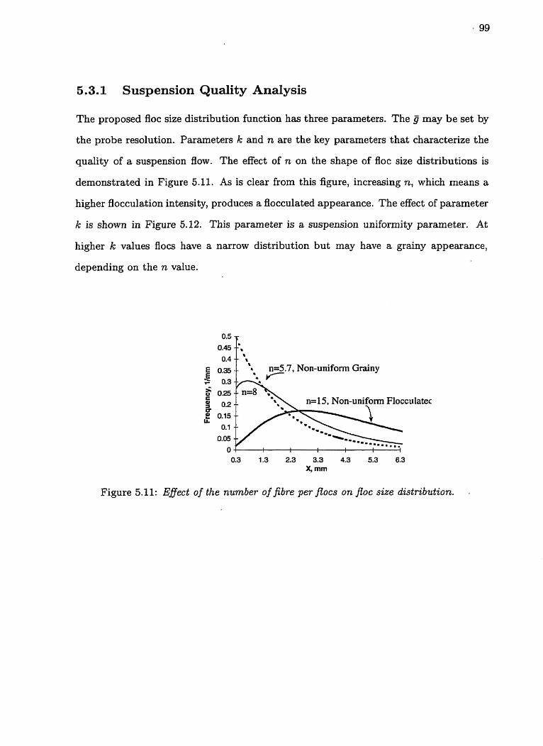
5.3.1 Suspension Quality Analysis

The proposed floc size distribution function has three parameters. The g may be set by

the probe resolution. Parameters k and n are the key parameters that characterize the

quality of a suspension flow. The effect of n on the shape of floc size distributions is

demonstrated in Figure 5.11. As is clear from this figure, increasing n, which means a

higher flocculation intensity, produces a flocculated appearance. The effect of parameter

k is shown in Figure 5.12. This parameter is a suspension uniformity parameter. At

higher k values flocs have a narrow distribution but may have a grainy appearance,

depending on the n value.

on-uniform Grainy

0 I I I I I

0.3 1.3 2.3 3.3 4.3 5.3 6.3 X, rnm

Figure 5.11: Effect of the number of fibre per fZocs on floe size distribution. .

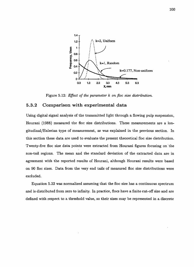
12 t , . j: k=2, Uniform I .

Figure 5.12: Effect of the parameter k on floe size distribution.

5.3.2 Comparison with experimental data

Using digital signal analysis of the transmitted light through a flowing pulp suspension,

Hourani (1988) measured the floc size distributions. These measurements are a lon-

gitudinal/Eulerian type of measurement, as was explained in the previous section. In

this section these data are used to evaluate the present theoretical floc size distribution.

Twenty-five floc size data points were extracted from Hourani figures focusing on'the

non-tail regions. The mean and the standard deviation of the extracted data are in

agreement with the reported results of Hourani, although Hourani results were based

on 90 floc sizes. Data from the very end tails of measured floc size distributions were

excluded.

Equation 5.22 was normalized assuming that the floc size has a continuous spectrum

and is distributed from zero to infinity. In practice, flocs have a finite cut-off size and are

defined with respect to a threshold value, so their sizes may be represented in a discrete

form. Taking this into consideration, Hourani's data were analyzed using a method

similar to the that suggested by (Levenspiel, 1972) in the context of characterizing non-

ideal flow of reacting systems.

To estimate the parameters of the present model, it is assumed that corresponds

to the resolution of the probe used for measuring floc sizes. The model parameters, a

and b, were estimated from matching the mean and standard deviation of the Equation

( 5.23) with those extracted from the Houarni figures. For all cases of flocculation

data plotted in the Hourani's paper, the model equations were in good agreement with

experimental data. Figures (5.13) to (5.16) are the results of these comparisons. The

estimated model parameters through these Figures are listed in Table 5-3. There is

little variation associated with the parameter n. This means that we could have set

n = 6 and adjusted the parameter k and still get a good fit. The choice of n x 6

resembles a definition for the fibre fiocs in Hourani's experiment and should correspond

to the mean values of the measuring probe signal. Hourani proposed a model to fit to

his experimental data. Figure 5.17 compares Hourani's theoretical model influenced by

13.7 coulombs/m2 charge density with the model presented in this work.

5.4 Closure

Non-intrusive Lagrangian measurements of the scale of flocculation in the plane normal

to the main flow of relevant paper forming consistencies are extremely difficult. A

novel model was developed to predict floc size distributions in such flows. The model

presupposes a 2-D random walk structure for the flocs for which a general floc size

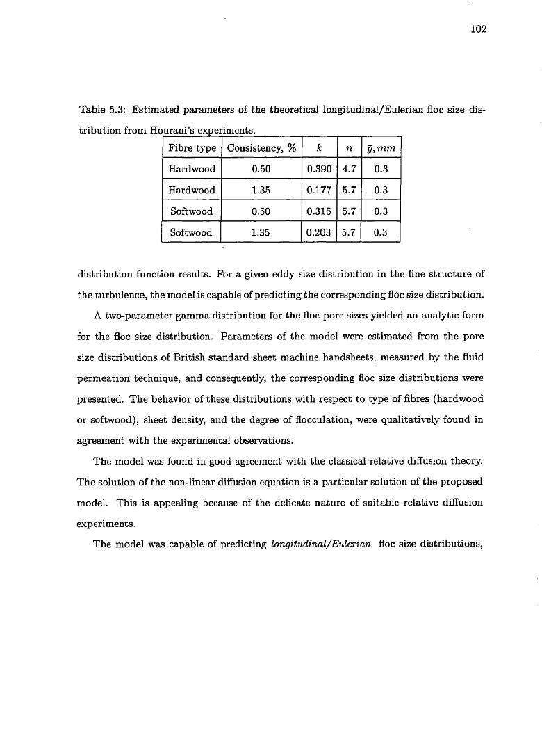
Table 5.3: Estimated parameters of the theoretical longitudinal/Eulerian floc size dis-

tribution from Hourani's experiments.

distribution function results. For a given eddy size distribution in the fine structure of

the turbulence, the model is capable of predicting the corresponding floc size distribution.

A two-parameter gamma distribution for the floc pore sizes yielded an analytic form

for the floc size distribution. Parameters of the model were estimated from the pore

size distributions of British standard sheet machine handsheets, measured by the fluid

permeation technique, and consequently, the corresponding floc size distributions were

presented. The behavior of these distributions with respect to type of fibres (hardwood

or softwood), sheet density, and the degree of flocculation, were qualitatively found in

agreement with the experimental observations.

The model was found in good agreement with the classical relative diffusion theory.

The solution of the non-linear diffusion equation is a particular solution of the proposed

model. This is appealing because of the delicate nature of suitable relative diffusion

experiments.

The model was capable of predicting longitudinal/Eulerian floc size distributions,

which were in good agreement with experimentally measured floc size distributions.

- Model Exp. data

0.3 1.3 2.3 3.3 4.3 5.3 6.3 X, rnm

Figure 5.13: Comparison between the theoretical floe size distribution and experimental

data for hardwood fibres at consistency 1.35%.

Exp. data - Model

Figure 5.14: Comparison between the theoretical floe size distribution end experimental

data for hardwood fibres at consistency 0.5%.

+ Experimental Data - Model

Figure 6.15: Comparison between the theoretical jloc size distribution and experimental

data for sofiwood fibres a t consistency 0.5%.

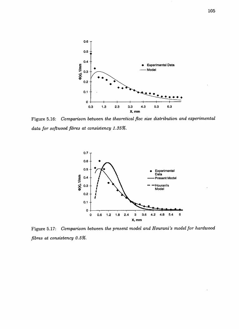
+ Experimental Data - Model

Figure 5.16: Comparison between the theoretical fEoc size dzstrzbution and experimental

data for softwood fibres at consistency 1.35%.

+ Experimental Data - Present Model

- - Hourani's Model

Figure 5.17: Comparison between the present model and Hourani's model for hardwood

fibres at consistency 0.5%.

Chapter 6

Conclusions

In this thesis a new device was developed to measure and characterize fibre flocculation

in a suspension flowing through a grid generated turbulence channel (turbulence rig)

flow. A semi-bleached kraft hardwood pulp fibres was used in all experiments. The

production and decay of turbulence behind the grids resembled common papermaking

flows adjacent to rectifiers, pressure screens, flow distributors, and headbox slices. The

local mass variability, measured over a small constant area, was found to be a reliable

but not a sufficient parameter to characterize quality of a suspension flow. Consequently,

the scale dependency of fibre flocculation was characterized by statistical modeling of

floc size distributions in turbulent flows.

6.1 Flow/Mass Variability Analysis

Different types of flows produced in the rig and their influences on fibre flocculation were

characterized as follow:

1. The grids were found to generate turbulence kinetic energy, and consequently

reduced flocculation.

2. The decay of turbulence kinetic energy began to occur a t x / d = 8.5 downstream

from the grids, which enhanced fibre flocculation.

3. Grids produced a non-homogeneous cross flow direction flocculation profiles, but

suspension homogeneity increased further downstream of the grids.

4. An irrotational shearing action at the grid exit was found, almost always, to disrupt

flocs, and the local mass variability was found to reach a minimum value. This

type of flow field was generated in the interface between a jet issuing from a grid

and the low velocity flow field behind that grid.

5. Two rotational shear flow cells developed behind each grid, and fibre flocculation

was found to be highest in the centre of rotations.

6. An increase in flow velocity was found to decrease the flocculation intensity. The

effect of mean concentration within the papermaking ranges of 0.45-0.75%, how-

ever, was found to be anomalous: an increase in the concentration resulted in a

decrease in the flocculation intensity. This was attributed to the high mobility of

the short fibres used in this study.

7. For characterizing fibre aggregation phenomenon in decaying turbulent flows, a

model was proposed and found to be in agreement with experimental data.

6.2 Flow/Floc Scale Analysis

The mass variability was found to be a necessary but not sufficient parameter in charac-

terizing the quality of a flowing suspension. The measured values of the mass variability

did not say anything about the suspension appearance in terms of graininess or size of

flocs. Two complementary parameters, which identify floc size distributions, were intro-

duced t o account for the scale uniformity of a suspension flow. In practice, non-intrusive

measurements of the scale of the fibre flocculation in the plane perpendicular t o the

main flow of relevant paper forming consistencies are extremely difficult. A novel model.

was developed to predict floc size distributions in such flows.

For a given eddy size distribution in the fine structure of the turbulence produced

inside of a flocculated structure, the model was found to be capable of predicting the

corresponding Aoc size distribution. Using the two-parameter gamma distribution for the

floc pore sizes, an analytic form for the floc size distribution was obtained. Parameters

of the model were estimated from the pore size distributions of British handsheets,

measured by the fluid permeation technique, and consequently, the corresponding floc

size distributions were estimated. The behavior of these distributions with respect to

the type of fibres (hardwood or softwood), sheet density, and the degree of flocculation,

were qualitatively found in agreement with experimental observations. The model was

found in good agreement with the classical relative diffusion theory. The solution of the

non-linear diffusion equation was a particular solution of the proposed model. This is

appealing because of the delicate nature of suitable relative diffusion experiments for

obtaining Aoc size distributions in complex flows.

The model was capable of predicting longitudinal/Eulerian floc size distributions and

found to be in good agreement with experimentally measured floc size distributions. The

behavior of these distributions with respect to parameters affecting suspension quality

was presented.

Implementation

The parameters determining paper quality both in terms of mass non-uniformity and the

scale for which this non-uniformity occurs are strongly influenced by the history of pulp

suspension passing through a headbox. Since there is a number of decaying turbulence

regions within a headbox, characterizing flocculation in a turbulent decaying flow field

may have a great impact on the headbox design. For example, in a typical headbox, a

turbulent decaying flow is generated in the stilling chamber by stepped diffusers. Flow

inside the diffusers is itself a turbulent decaying flow.

Turbulence in a headbox causes dispersion of fibre aggregates but the decay of tur-

bulence enhances re-flocculation of the dispersed fibres downstream of a turbulence gen-

erator. In order to disperse flocs in a turbulent decaying flow field, a converging channel

section is connected to the turbulence generator device. The length, convergence ratio,

the turbulence generator system itself, pulp type and concentration, and flow velocity

are the key design parameters, which determines the quality of a suspension flow issu-

ing from the slice. An accelerating flow produces an elongational flow, which causes

disruption of flocs and orienting fibres along the main flow direction while decay of tur-

bulence promotes flocculation. Therefore, there is a simultaneous competition between

aggregation and disruption of flocs. The work presented in Chapter 4 was focused on

characterizing the flocculation process. Further work is needed to model floc disruption

process in an eloagational flow field. Once the latter is known, i t can be combined

with the present flocculation model to provide a useful tool for designing the complex

geometry of a headbox.

In Chapter 5 models were proposed t o characterize floc size distribution. Floc size

distributions were found to be characterized by two process controlling parameters n and

k. These parameters characterize the graininess and uniformity, respectively. Parameter

n is related to the flocculation intensity and hence to the flocculation model proposed

in Chapter 4. However, further work is required t o relate k to the flow condition.

Nevertheless, i t is postulated that the parameter k is proportional to the extent of floc

disruption and therefore, can be correlated to the elongational flow characteristics in the

headbox, jet/wire speed. If all these conditions are fixed, then k may only depend on

the pulp consistency. In practice, i t is possible to determine these parameters from the

measured floc size distribution of the paper produced and consequently, by varying the

headbox flow and/or geometry condition to achieve the desired paper product.

6.4 Recommendat ions

It is recommended that the DPV system developed in this work should be used to study

the effects of the following parameters on fibre flocculation:

1. Fibre type (softwood) and fibre length,

2. Different grid geometries, and various flow cells, e.g. converging and diverging flow

fields,

3. Combined grid generated turbulence and elongation flow.

The results of the present work together with the results of the above experiments should

be used to simulate papermaking flows using CFD approach.

Appendix A

Flocculation intensity data

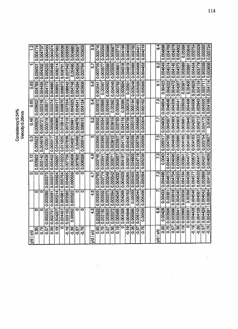
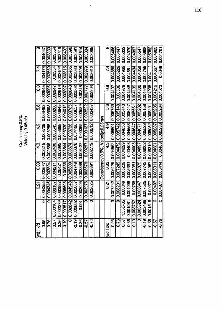
References

Adrian, R.J. (1991). Particle-Imaging techniques for experimental fluid mechanics.

Ann. Rev. Fluid Mech., 23,261-304.

Aiden, C.K. and Kovacs, A.E. (1995). Hydrodynamics of the forming sections: the

origin of nonuniformity fibre orientation. Tappi J., 78 (1 I ) , 97-106.

Anderson, 0. (l.966). Some observations on fibre suspensions in turbulent motion.

Svenslc Papperstid., 69(2) ,23-3 1.

Bakker, A., Fasano, J.B., and Leng, D.E. (1994). Pinpoint mixing problems with lasers

and simulation software. 'Chemical Engineering, Jan., 95-100.

Batchelor, B.K. and Townsend, A.A. (1948) Pro. Roy. Soc., London, 199A, 238.

Bliesner, W.C. (1964). A study of the porous structure of fibrous sheets using perme-

ability techniques. Tappi , 47(7), 129-144.

Bonano, E.J. (1984). A study of Aoc break up and formation in flowing concentrated

fiber suspensions. Int. J. Multzphase Flow, 10(5), 623-633.

Chatterjee, A. (1995). P hysic-chemical aspects of flocculation in cellulose fi-

bre sispension and effects o n paper formation, Ph.D. Thesis, University of

Toronto.

Corte, H. and Lloyd, E.H. (1965). Fluid flow through paper and sheet structure. In

Consolidation of the Paper Web, Trans. Fund. Res. Syrnp., Cambridge, F . Bolam.,

Ed., Tech. Sec. BPBMA, London, 981-1009.

d71ncau, S. (1983). Characterization of the decay of turbulence in a pulp suspension

flow. Tappi Proceedings, 1989 Engineering Conference, 583-592.

Deng, M. and Dodson, C.T. J. (1994). Paper: An Engineered Stochastic Struc-

ture. Tappi press, Atlanta.

Dodson, C.T.J. and Schaffnit, C. (1992). Flocculation effects on formation statistics.

Tappi J., 75(1), 167-174.

Dodson, C.T. J . (1996). Fibre crowding, fibre contacts, and fibre flocculation. Tappi

J., 79(9), 211-216.

Dodson, C.T.J. and Sampson, W.W. (1996). The effect of paper formation and gram-

mage on its pore size distribution. J. Pulp Paper Sci., 22(5), 5165-3169.

Erdelyi, A. (1961). General asymptotic expansions of Laplace integrals. Arch. Rational

Mech. Anal., 7, 1-20.

Farnood, R.R. (1995). Sensing and modeling of forming and formation of

paper. Ph.D. Thesis, University of Toronto.

Farnood, R.R. and Dodson, C.T.J. (1995). The similarity law of formation. In Pro-

ceedings of Internatzonal Conference on Paper Physics, Niagara-on-the-Lake, 5-12.

Gad-El-Hak, M. and Corrsin, S. (1974). Measurements of the nearly isotropic turbu-

lence behind a uniform jet grid. J. Fluid Mech., 2, 115-143.

Hentschel, H.G. and Procaccia, I. (1983). Relative diffusion in turbulent media: The

fractal dimension of clouds. Phys. Rev. A, 29, 1461- 1470.

Hinze, J.O. (1975). Zhrbulence. 2nd Edition, McGraw-HILL.

Hourani, M.J. (1989). Fibre flocculation in pulp suspension fiow. Part 1: theoretical

model. Tappi J., 71(5), 115-118.

Hourani, M. J. (1989). Fibre flocculation in pulp suspension flow. Part 2: experimental

results. Tappi J., 71 ( 6 ) , 186-189.

Ilmoniemi, E., Aroviita, L., and Yci-Kokko, E. (1986). The roIe of headbox turbulence

generators in grammage uniformity. Appita, 39 (I), 36-40.

Jahne, B. (1997). Practical handbook on image processing for scientific appli-

cations. Boca Raton, F1a:CRC.

Jones, G.L. and Ginow, R. J. (1988). Modeling headbox performance with computa-

tional fluid mechanics. Tappi Proceedings, 1988 Engineering Conference, 15-20.

Kaji, H., Monma, K., and Katsura (991). Fractal analysis of flocculation in pulp

suspension. In Proc. International Paper Physics Conference, Kona, Hawaii, 291-

297.

Kao, S.V. and Mason, S.G. (1975). Dispersion of particles by shear. Nature, 253,

619-621.

Kerekes, R. J., (1979). High turbulence for headboxes questioned. Pulp Paper Can.,

80(9), 31-32.

Kerekes, R. J. and Garner, R.G. (1982). Measrernents of turbulence in pulp suspensions

by laser anemometry. J. Pulp Paper Sci., 8(3), TR53-TR59.

Kerekes, R.J. (1983). Pulp floc behavior in entry flow to constrictions. Tappi J. , 66(1),

88-91.

Kerekes, R. J. (1983). Pulp flocculation decaying turbulence: a literature review. J.

Pulp Paper Sci., 9(3), TR86-TR91.

Kerekes, R.J., Soszynski, R., and Tam Doo, P. (1985). The flocculation of pulp fi-

bres. B+ansactions of the Eight Fundamental Research Symposium, Oxford, 1,

265-510. Ed. V. Panton, Papermaking Raw Materials - Their interaction with the

production process and their effect on paper properties. Mechanical ~ n ~ i n e e i i n ~

Productions Limited, London.

Kerekes, R.J. and Schell, C.J. (1992). Characterization of fibre flocculation regimes by

a crowding factor. J. Pulp Paper Sci., l8( l ) , 532-538.

Kletle, R. (1996). Handbook of image processing operators. WILEY, New York.

Levenspiel, 0. (1972). Chemical reaction engineering. 2nd Edition, John Wiley &

Sons, Inc., New York.

Lin, J.Y. (1988). A numerical study on turbulent flow through a circular step diffuser.

Tappi Proceedings, 1988 Engineering Conference, 21-29.

Mason, S.G. (1950). The flocculation of pulp suspensions and the formation of paper.

TA PPI, 33 (9), 440-444.

Mason, S.G. (1954). Fibre motions and flocculation. Pulp paper Mag. Can., 55(13),

96-102.

Meyer, R. and Wahren, D. (1965). Svensk Papperstid., 68(lO), 432-436.

Mohamed, S.M. and LaRue, J.C. (1990). The decay power law in grid-generated tur-

bulence. J. Fluid Mech., 219, 195-214.

Nerelius, L., Norman, B., and Wahren, D. (1972). Measurements of flocculation char-

acteristics by light reflection. Tappi J., 55(4), 574-580.

Norman, B. and Wahren, D. (1972). A comprehensive method for the description of

mass distribution in sheets and flocculation and turbulence in suspensions. Svensk

Papperstidning, 75 (20) ,807-818.

Norman, B.G., Mijller, K., Ek, R., and Duffy, D.G. (1989). Hydrodynamics of Paper-

making Fibres in Water Suspension, in Fibre-Water Interactions in Papermaking.

lPransactions of the Symposium held in Oxford. BPBIF, 195-246.

O'Shaughnessy, B. and Procaccia, I. (1984). Analytical solutions for diffusion on fractal

objects. Phys. Rev. Lett., 54(5), 455.

Oshinowo, O.M. (1997). Flow modifying screens in turbulent flows. an appli-

cation to pulverized coal-fired boilers. Ph.D. Thesis, University of Toronto.

Parker, J. and Herhert, D. (1968). Simultaneous convergence - a new concept of head-

box design. Tappi, 51(10), 452-432.

Persinger, L. and Meyer, H. (1975). Scale of flocculation for fully developed turbulent

tube flow of dilute fibre suspensions Papper ja Puu, 57(9), 563-577.

Rayleigh, Lord (1919). On the problem of random vibrations, and of random flights in

one, two, or three dimensions. Philosophical Magazine, 37, 321-347.

Richardson, L.F. (1926). Proc. R. Soc., London, Ser. A, 110, 709.

Rital, R. and Huiku, M. (1989). Scaling, percolation and network theories; new insights

into papermaking. l?ransactions of the ninth fundamental research symposium,

Cambridge, vol. 3, 163-1 67. Ed. C.F. Baker, Fundamental of papermaking,

Mechanical Engineering Publications Limited, London.

Roach, P.E. (1986). The generation of nearly isotropic turbulence by means of grids.

Int. J. Heat & Fluid Flow, 8 , 82-92.

Roach, P.E. (1986). The generation of nearly isotropic turbulence downstream of

stream wise bundles. Int.' J. Heat & Fluid Flow, 7, 82-92.

Robertson, A.A. and Mason, S.G. (1954). Flocculation in flowing pulp suspensions.

Pulp Pap. Mag. Can., 55(3), 263-269.

Sanders, H.T. and Meyer, H. (1971). Consistency distribution in turbulent tube flow

of fibre suspensions. Tappi J., 54(5), 722-730.

Schaffrath, H. J. and Gbttsching, L. (1991). The behavior of paper under compression

in the z-direction. In Proc. Tappi International Paper Physics Conference, Kona,

489-510.

Smith, M.K. (1986). Formation potential of west coast kraft pulps. Pulp & Paper

Canada, 87(10), 69-76.

Smith, W. J. (1990). Modern optical engineering. McGRAW HILL, NEW YORK.

Soszynski, R.M. and Kerekes, R. J. (1988). Elastic interlocking of nylon fibres suspended

in liquid: Part 1 Nature of cohesion among fibres. Noridic Pulp and Paper Res.

J., 3(4), 172-179.

Soszynski, R.M. and Kerekes, R. J. (1989). Elastic interlocking of nylon fibres suspended

in liquid: Part 2 Process of interlocking. Noridic Pulp and Paper Res. J., 3(4),

180.

Steen, M. (1989). On turbulence structure in vertical pipe flow of fibre suspensions.

Noridzc Pulp & Paper Res. J., 4, 244-252.

Steen, M. (1991). Modelling fibre flocculation in turbulent flow: a numerical study.

Tappi J., 74(4), 175-182.

Steen, M. (1992). Fibre flocculation in turbulent flow. Proc. PIRA Conference on

Flocculatzon Control, Luxembourg. PIRA International, Leatherhead, U.K., 1-25.

Takeuchi, N. et.al. (1983). Formation and destruction of fibre flocs in a flowing pulp

suspension. Appita, 37(3), 223-230.

Tam DQO, P.A., Kerekes, R.J., and Pelton, R.H. (1984). Estimates of maximum hydro-

dynamic shear stresses on fibre surface in papermaking. J. Pulp Paper Sci., 10(4),

580- 588.

Tan-Atichat, H.M., Nagib, H.M., and Loehrke, R.I. (1982). Interaction of free-stream

turbulence with screen and grids: a balance between turbulence scales. J. Fluid

Mech., 114, 501-528.

Van Den Akker, J.A. (1954). Flow in fibre suspensions and the effects of turbulence.

Pulp Paper Mag. Can., 55(13), 91-96.

Wahren, D. (1967). Proposed definitions of some basic papermaking terms. Suensk

Papperstidning, 70 (21) ,725.

Weiss, G.H. (l994). Aspects and applications of the random walk. North -

Holland.

Wollwage, J.C. (1940). Paper Trade J. , 108(12), 41-48.

Wong, G.H. (1989). Asmptotic approximations of integrals. Academic Press,

New York.

Wrist, P.E. (1962). Dynamics of sheet formation on the fourdrinier machine. In Pro-

ceedings of the Symposium Held at Oxford, England (1961), 2, 839-899. Ed. F.

Bolam. Technical Section of the British and Board Makers' Association, London.