Characterization of MEMS Electrostatic Actuators … · Characterization of MEMS Electrostatic...
76
Characterization of MEMS Electrostatic Actuators Beyond Pull-In A Thesis Submitted for the Degree of Master of Science (Engineering) in Faculty of Engineering by Gorthi V.R.M.S. Subrahmanyam Supercomputer Education and Research Centre Indian Institute of Science Bangalore – 560 012 (INDIA) JANUARY 2006
Transcript of Characterization of MEMS Electrostatic Actuators … · Characterization of MEMS Electrostatic...

Characterization of MEMSElectrostatic Actuators Beyond
Pull-In
A Thesis
Submitted for the Degree of
Master of Science (Engineering)
in Faculty of Engineering
by
Gorthi V.R.M.S. Subrahmanyam
Supercomputer Education and Research CentreIndian Institute of Science
Bangalore – 560 012 (INDIA)
JANUARY 2006

Acknowledgments
I would like to express my immense gratitude to my adviser Dr. Atanu Mohanty, who
supported me greatly and did every possible effort to teach and help me. I am more than
thankful to him for patiently educating me. He is probably the best teacher I have ever
come across. He gave complete freedom and helped me in all aspects. I am very happy
to be blessed with such a care taking, friendly and knowledgeable guide.
I am indebted to Dr. Anindya Chatterjee for his guidance and parental care. He guided
in many aspects of this work particularly, the chapter on dynamic analysis is a result of
his guidance. The interactions with him are very informative and pleasant memories for
ever. I am inspired by his attitude, workaholic nature and concern for others. Most of
my learning in IISc is from these two teachers.
I would like to thank Prof. S. K. Sen for his encouragement. I am thankful to Dr.
Sayanu for the lectures on MEMS and introducing some of the basic concepts of MEMS.
The discussions that I had with him are very helpful. I wish to thank Dr. K. J. Vinoy for
the useful course work on Antennas and MEMS. He is always very kind and helpful to me.
I am thankful to Dr. G. K. Ananthasuresh for allowing me to attend his course on MEMS
and also for going through the manuscript of the paper patiently and making suggestions.
I thank Dr. Raha for teaching me data structures. Thanks are due to the Chairman of our
department for his support. I am thankful to my friends Prasad, Rajan, Surya, Rupesh,
Ashok, Rahul, Jay, Sangamesh, Vivek and many others. I would like thank all the staff of
SERC for their friendliness and cooperation. Thanks to all the people who are involved
in the development of Linux, Latex, LyX, and Dia.
Last but not the least, I am indebted to my parents, sisters: Lalitha, Radha, and my
i

ii
brother: Sai Siva. The care, love and affection of them are responsible for my present
stage. I am thankful to the God for pouring His love through all these people.
All these things became possible in my life only because of the inspiration, guidance
and support of Sri P. Subbaramaih sir of Golagamudi, I would like to express my heart-felt
gratitude to Sri Subbaramaih Sir. Finally and most importantly, I offer my pranamas to
the lotus feet of Sri Ekkirala Bharadwaja master, Sai Baba of Shirdi, and Bhagavan Sri
Venkaiah Swamy of Golagamudi.

Abstract
The operational range of MEMS electrostatic parallel plate actuators can be extended be-
yond pull-in with the presence of an intermediate dielectric layer, which has a significant
effect on the behaviour of such actuators. Here we study the behaviour of cantilever beam
electrostatic actuators beyond pull-in using a beam model along with a dielectric layer.
Three possible static configurations of the beam are identified over the operational voltage
range. We call them floating, pinned and flat: the latter two are also called arc-type and
S-type in the literature. We compute the voltage ranges over which the three configu-
rations can exist, and the points where transitions occur between these configurations.
Voltage ranges are identified where bi-stable and tri-stable states exist. A classification
of all possible transitions (pull-in and pull-out as well as transitions we term pull-down
and pull-up) is presented based on the dielectric layer parameters. A scaling law is found
in the flat configuration. Dynamic stability analyses are presented for the floating and
pinned configurations. For high dielectric layer thickness, discontinuous transitions be-
tween configurations disappear and the actuator has smooth predictable behaviour, but
at the expense of lower tunability. Hence, designs with variable dielectric layer thickness
can be studied in future to obtain both regularity/predictability as well as high tunability.
iii

Contents
Abstract iii
Publications based on this Thesis ix
1 Introduction 11.1 Background and Motivation . . . . . . . . . . . . . . . . . . . . . . . . . . 11.2 MEMS Parallel Plate Electrostatic Actuators . . . . . . . . . . . . . . . . . 3
1.2.1 Simple Lumped-Element Model . . . . . . . . . . . . . . . . . . . . 31.2.2 Pull-in Voltage . . . . . . . . . . . . . . . . . . . . . . . . . . . . . 41.2.3 Deflection . . . . . . . . . . . . . . . . . . . . . . . . . . . . . . . . 51.2.4 Applications . . . . . . . . . . . . . . . . . . . . . . . . . . . . . . . 71.2.5 Limitations of Lumped Model . . . . . . . . . . . . . . . . . . . . . 10
1.3 Thesis Organization . . . . . . . . . . . . . . . . . . . . . . . . . . . . . . . 10
2 Mathematical Modeling and Simulations 122.1 Introduction . . . . . . . . . . . . . . . . . . . . . . . . . . . . . . . . . . . 122.2 Possible Configurations . . . . . . . . . . . . . . . . . . . . . . . . . . . . . 122.3 Governing Equation . . . . . . . . . . . . . . . . . . . . . . . . . . . . . . 142.4 Normalized Equation . . . . . . . . . . . . . . . . . . . . . . . . . . . . . . 152.5 Modal Expansion Method . . . . . . . . . . . . . . . . . . . . . . . . . . . 17
2.5.1 Modal Expansion Method in General . . . . . . . . . . . . . . . . . 172.5.2 Floating Configuration . . . . . . . . . . . . . . . . . . . . . . . . . 202.5.3 Pinned Configuration . . . . . . . . . . . . . . . . . . . . . . . . . . 222.5.4 Procedure to Solve the Coupled Equation . . . . . . . . . . . . . . 242.5.5 Modified Procedure using Newton’s Method . . . . . . . . . . . . . 25
2.6 Finite Difference Approximation . . . . . . . . . . . . . . . . . . . . . . . . 312.6.1 Method . . . . . . . . . . . . . . . . . . . . . . . . . . . . . . . . . 312.6.2 Floating Configuration . . . . . . . . . . . . . . . . . . . . . . . . . 332.6.3 Pinned Configuration . . . . . . . . . . . . . . . . . . . . . . . . . . 342.6.4 Flat Configuration . . . . . . . . . . . . . . . . . . . . . . . . . . . 36
2.7 Scaling Law in the Flat Configuration . . . . . . . . . . . . . . . . . . . . . 372.8 Discussion and Conclusions . . . . . . . . . . . . . . . . . . . . . . . . . . 38
iv
CONTENTS v
3 Effects of Dielectric Layer 403.1 Introduction . . . . . . . . . . . . . . . . . . . . . . . . . . . . . . . . . . . 403.2 Normalized Voltage (V ) Limits of Configurations . . . . . . . . . . . . . . 403.3 Transitions . . . . . . . . . . . . . . . . . . . . . . . . . . . . . . . . . . . . 41
3.3.1 Pull-In . . . . . . . . . . . . . . . . . . . . . . . . . . . . . . . . . . 433.3.2 Pull-Down . . . . . . . . . . . . . . . . . . . . . . . . . . . . . . . . 443.3.3 Pull-Up . . . . . . . . . . . . . . . . . . . . . . . . . . . . . . . . . 443.3.4 Pull-out . . . . . . . . . . . . . . . . . . . . . . . . . . . . . . . . . 45
3.4 Bi-stability . . . . . . . . . . . . . . . . . . . . . . . . . . . . . . . . . . . 453.5 Discussion and Conclusions . . . . . . . . . . . . . . . . . . . . . . . . . . 46
4 Dynamic Stability of Equilibrium Solutions 484.1 Introduction . . . . . . . . . . . . . . . . . . . . . . . . . . . . . . . . . . . 484.2 Method . . . . . . . . . . . . . . . . . . . . . . . . . . . . . . . . . . . . . 484.3 Stability Results . . . . . . . . . . . . . . . . . . . . . . . . . . . . . . . . 524.4 Discussion and Conclusions . . . . . . . . . . . . . . . . . . . . . . . . . . 53
5 Case Study 55
6 Conclusions and Further Work 61
Bibliography 62
List of Tables
2.1 Boundary conditions at the free end of the cantilever beam for the threeconfigurations. . . . . . . . . . . . . . . . . . . . . . . . . . . . . . . . . . . 14
2.2 Description of the parameters in the governing equation. . . . . . . . . . . 152.3 Roots and coefficient values of various modes of the floating configuration. 212.4 Roots and coefficient values of various modes of the pinned configuration. . 232.5 Characteristic equations, coefficient values and Initial position of the beam
for various configurations. . . . . . . . . . . . . . . . . . . . . . . . . . . . 24
5.1 Dimensions and material properties of a MEMS actuator. . . . . . . . . . . 55
vi

List of Figures
1.1 Simple lumped-element model of MEMS electrostatic parallel plate actua-tor with 1 degree of freedom . . . . . . . . . . . . . . . . . . . . . . . . . . 3
1.2 Solutions of MEMS electrostatic actuator without dielectric layer . . . . . 71.3 Solutions of MEMS electrostatic actuator for different dielectric layer thick-
ness values . . . . . . . . . . . . . . . . . . . . . . . . . . . . . . . . . . . . 81.4 C-V characteristics of MEMS electrostatic actuator for different dielectric
layer thickness values . . . . . . . . . . . . . . . . . . . . . . . . . . . . . . 9
2.1 Schematic view of the cantilever beam electrostatic actuator. . . . . . . . . 132.2 Possible configurations of the cantilever beam actuator. (The scale in the
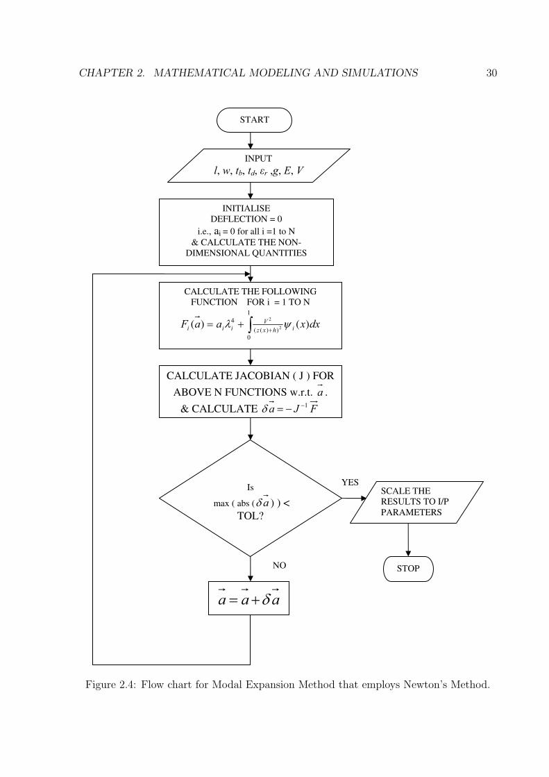
vertical direction is exaggerated.) . . . . . . . . . . . . . . . . . . . . . . . 142.3 Flow chart for Modal Expansion Method. . . . . . . . . . . . . . . . . . . . 262.4 Flow chart for Modal Expansion Method that employs Newton’s Method. . 302.5 Flow chart for Finite difference approximation of floating and pinned con-
figurations. . . . . . . . . . . . . . . . . . . . . . . . . . . . . . . . . . . . 35
3.1 V limits of the three configurations. . . . . . . . . . . . . . . . . . . . . . . 423.2 Classification of possible transitions based on the numerical results of Fig. 3.1. 423.3 Variation of the magnitude of the pull-in discontinuity with h. . . . . . . . 433.4 Pull-down: jump in slope at the touching end of the beam. . . . . . . . . . 443.5 Variation of the magnitude of the pull-down discontinuity with h. . . . . . 453.6 Variation of width of bi-stability region with h. . . . . . . . . . . . . . . . 46
4.1 Stability analysis of the floating configuration. . . . . . . . . . . . . . . . . 524.2 Stability analysis of the pinned configuration. . . . . . . . . . . . . . . . . 53
5.1 Floating configuration: Variation of height at the free end of the beam withapplied voltage. . . . . . . . . . . . . . . . . . . . . . . . . . . . . . . . . 56
5.2 Pinned configuration: Contact force at the touching end of the beam vs.applied voltage. . . . . . . . . . . . . . . . . . . . . . . . . . . . . . . . . . 57
5.3 Pinned configuration: Slope at the contact point of the cantilever beam vs.applied voltage. . . . . . . . . . . . . . . . . . . . . . . . . . . . . . . . . . 58
5.4 Flat configuration: Contact length of the cantilever beam with the dielec-tric layer vs. applied voltage. . . . . . . . . . . . . . . . . . . . . . . . . . . 59
5.5 Voltage ranges of the three configurations. . . . . . . . . . . . . . . . . . . 59
vii

LIST OF FIGURES viii
5.6 C-V characteristics in the floating configuration. . . . . . . . . . . . . . . . 605.7 C-V characteristics in the flat configuration. . . . . . . . . . . . . . . . . . 60
6.1 Proposed designs to achieve more regular and reversible behaviour as wellas higher tunability . . . . . . . . . . . . . . . . . . . . . . . . . . . . . . . 61
Publications based on this Thesis
• Subrahmanyam Gorthi, Atanu Mohanty and Anindya Chatterjee, “Cantilever
beam electrostatic MEMS actuators beyond pull-in,” in Journal of Micromechanics
and MicroEngineering, vol. 16, num. 9, 1800-1810, 2006.
• Subrahmanyam Gorthi, Atanu Mohanty and Anindya Chatterjee, “MEMS par-
allel plate actuators: pull-in, pull-out and other transitions,” presented in Interna-
tional Conference on MEMS and Semiconductor Nanotechnology, December 20-22,
IIT Kharagpur, India.
ix

Chapter 1
Introduction
This thesis presents a study of cantilever beam MEMS electrostatic actuators beyond pull-
in. The effects are studied of an intermediate dielectric layer on the possible configurations
of the actuator and transitions between them.
1.1 Background and Motivation
MEMS (Micro-Electro-Mechanical-Systems) are the microscopic structures integrated onto
silicon (or similar substrate) that combine mechanical, optical, fluidic and other elements
with electronics. These devices enable the realization of complete system-on-a-chip.
MEMS make it possible for systems to be smaller, faster, more energy efficient, more
functional and less expensive. In a typical MEMS configuration, integrated circuits (ICs)
provide the “thinking part” of the system, while MEMS complement this intelligence with
active perception and control functions.
Electrostatic actuation is one of the most commonly used schemes for MEMS devices.
In MEMS electrostatic parallel plate actuators (discussed in detail in the next section),
the moving plate comes to equilibrium when the electrostatic force is balanced by the
restoring mechanical force. The restoring force increases (approximately) linearly with
deflection whereas the electrostatic force is inversely proportional to the square of the
distance between the plates. Due to this nonlinear nature of the electrostatic force, as
1
CHAPTER 1. INTRODUCTION 2
the moving plate traverses about one third of the total distance between the plates, the
restoring force can no longer be able to balance the electrostatic force and hence, the
moving plate (electrode) flaps onto the other plate. This is known as pull-in phenomena
and the corresponding voltage is called pull-in voltage.
Thus the operational range of MEMS electrostatic parallel plate actuators is limited by
the pull-in phenomena. The behaviour of the MEMS actuators before pull-in is studied
extensively in the literature [1–11]. With the presence of an intermediate dielectric
layer between the electrodes, the operational range can be extended beyond the pull-in
and they can be meaningfully modeled over the entire operational range. Many MEMS
devices operate beyond pull-in, e.g. capacitive switches [12, 13], zipper varactors [14, 15]
and CPW resonators [16]. However, the behaviour of MEMS devices beyond the pull-in
has not been studied in greater detail in the literature. This thesis presents a detailed
analysis of the cantilever beam MEMS electrostatic actuators, particularly beyond the
pull-in. The effects of an intermediate dielectric layer are also studied in detail and a
frame work of all possible types of transitions between the configuration is made based
on the dielectric layer thickness.
Simple lumped element models of MEMS actuators with a single degree of freedom
[17–20] result in easy calculations but fail to capture details of the behaviour beyond the
pull-in. At the other end of modeling complexities, simulations of MEMS actuators beyond
the pull-in have been done using 3-D models [21]. Similar approaches have been used in
studying the hysteresis characteristics of electrostatic actuators [22]. 3-D models [2,21,22]
lead to a detailed and accurate prediction, but simulations are expensive in time and
computation, particularly for problems involving mechanical contacts. In this thesis, we
employ a 1-D analysis that, at an intermediate level of complexity, gives useful results
with reasonable effort. Note that existing comparisons between 1-D and more detailed
models show that 1-D analysis can in fact provide useful results and insights [23,24].
The following section provides an introduction to MEMS electrostatic parallel plate
actuators with an intermediate dielectric layer between the electrodes, using a simple
lumped element spring-mass-damper model.
CHAPTER 1. INTRODUCTION 3
1.2 MEMS Parallel Plate Electrostatic Actuators
V
k
m
b
zg
Movable plate
Fixed ground plate
Dielectric layer
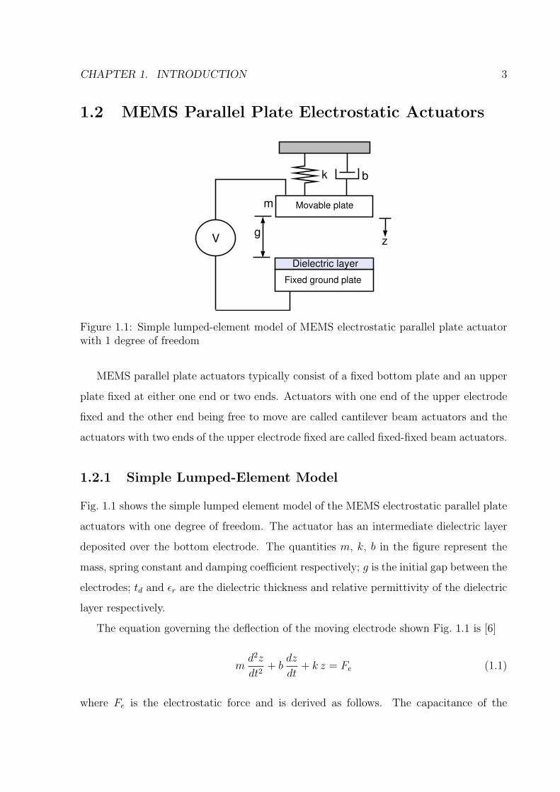
Figure 1.1: Simple lumped-element model of MEMS electrostatic parallel plate actuatorwith 1 degree of freedom
MEMS parallel plate actuators typically consist of a fixed bottom plate and an upper
plate fixed at either one end or two ends. Actuators with one end of the upper electrode
fixed and the other end being free to move are called cantilever beam actuators and the
actuators with two ends of the upper electrode fixed are called fixed-fixed beam actuators.
1.2.1 Simple Lumped-Element Model
Fig. 1.1 shows the simple lumped element model of the MEMS electrostatic parallel plate
actuators with one degree of freedom. The actuator has an intermediate dielectric layer
deposited over the bottom electrode. The quantities m, k, b in the figure represent the
mass, spring constant and damping coefficient respectively; g is the initial gap between the
electrodes; td and εr are the dielectric thickness and relative permittivity of the dielectric
layer respectively.
The equation governing the deflection of the moving electrode shown Fig. 1.1 is [6]
md2z
dt2+ b
dz
dt+ k z = Fe (1.1)
where Fe is the electrostatic force and is derived as follows. The capacitance of the

CHAPTER 1. INTRODUCTION 4
electrostatic actuator is
C =ε0A
g − z + tdεr
(1.2)
where A is area of the plate and ε0 is permittivity of free space. The effect of fringing is
not considered throughout in order to simplify the analysis. The electrical energy stored
in the parallel plate actuator is
E =1
2C V 2 =
ε0AV2
2(g − z + td
εr
) . (1.3)
The electrostatic force is
Fe =dE
dz=
ε0AV2
2(g − z + td
εr
)2 . (1.4)
Substituting Fe in Eq. 1.1,
md2z
dt2+ b
dz
dt+ k z =
ε0AV2
2(g − z + td
εr
)2 . (1.5)
When a DC potential is applied across the electrodes, at steady state, the above equation
reduces to
k z =ε0AV
2
2(g − z + td
εr
)2 . (1.6)
Note that the mechanical restoring force is given by the term on the left side of the above
equation and it varies linearly with deflection whereas the electrostatic force is given by
the right side term and is inversely proportional to the square of the deflection.
1.2.2 Pull-in Voltage
The expression for voltage, derived from Eq. 1.6 is
V =
√2 k
ε0Az
(g − z +
tdεr
)2
. (1.7)
CHAPTER 1. INTRODUCTION 5
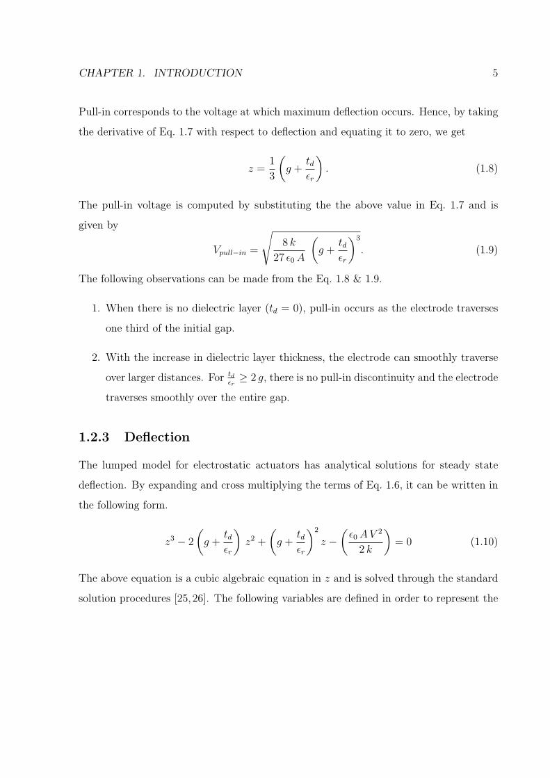
Pull-in corresponds to the voltage at which maximum deflection occurs. Hence, by taking
the derivative of Eq. 1.7 with respect to deflection and equating it to zero, we get
z =1
3
(g +
tdεr
). (1.8)
The pull-in voltage is computed by substituting the the above value in Eq. 1.7 and is
given by
Vpull−in =
√8 k
27 ε0A
(g +
tdεr
)3
. (1.9)
The following observations can be made from the Eq. 1.8 & 1.9.
1. When there is no dielectric layer (td = 0), pull-in occurs as the electrode traverses
one third of the initial gap.
2. With the increase in dielectric layer thickness, the electrode can smoothly traverse
over larger distances. For tdεr≥ 2 g, there is no pull-in discontinuity and the electrode
traverses smoothly over the entire gap.
1.2.3 Deflection
The lumped model for electrostatic actuators has analytical solutions for steady state
deflection. By expanding and cross multiplying the terms of Eq. 1.6, it can be written in
the following form.
z3 − 2
(g +
tdεr
)z2 +
(g +
tdεr
)2
z −(ε0AV
2
2 k
)= 0 (1.10)
The above equation is a cubic algebraic equation in z and is solved through the standard
solution procedures [25,26]. The following variables are defined in order to represent the
CHAPTER 1. INTRODUCTION 6
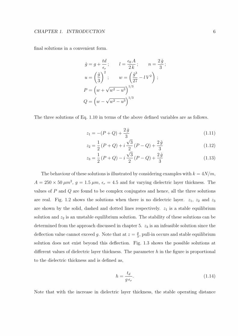
final solutions in a convenient form.
g = g +td
εr; l =
ε0A
2 k; n =
2 g
3;
u =
(g
3
)2
; w =
(g3
27− l V 2
);
P =(w +√w2 − u3
)1/3
Q =(w −√w2 − u3
)1/3
The three solutions of Eq. 1.10 in terms of the above defined variables are as follows.
z1 = −(P +Q) +2 g
3(1.11)
z2 =1
2(P +Q) + i
√3
2(P −Q) +
2 g
3(1.12)
z3 =1
2(P +Q)− i
√3
2(P −Q) +
2 g
3(1.13)
The behaviour of these solutions is illustrated by considering examples with k = 4N/m,
A = 250 × 50 µm2, g = 1.5 µm, εr = 4.5 and for varying dielectric layer thickness. The
values of P and Q are found to be complex conjugates and hence, all the three solutions
are real. Fig. 1.2 shows the solutions when there is no dielectric layer. z1, z2 and z3
are shown by the solid, dashed and dotted lines respectively. z1 is a stable equilibrium
solution and z2 is an unstable equilibrium solution. The stability of these solutions can be
determined from the approach discussed in chapter 5. z3 is an infeasible solution since the
deflection value cannot exceed g. Note that at z = g3, pull-in occurs and stable equilibrium
solution does not exist beyond this deflection. Fig. 1.3 shows the possible solutions at
different values of dielectric layer thickness. The parameter h in the figure is proportional
to the dielectric thickness and is defined as,
h =tdg εr
. (1.14)
Note that with the increase in dielectric layer thickness, the stable operating distance

CHAPTER 1. INTRODUCTION 7
increases and for h ≥ 2, the actuator traverses smoothly over the entire distance without
any discontinuity.
0 1 2 3 4 5 6 70
0.2
0.4
0.6
0.8
1
1.2
1.4
1.6
1.8
2
Applied Voltge (V)
Def
lect
ion
(µ m
)
VPullin
g
Stable
Unstable
Infeasible
g/3
Figure 1.2: Solutions of MEMS electrostatic actuator without dielectric layer
1.2.4 Applications
Two of the important applications of MEMS parallel plate actuators are as variable ca-
pacitors (varactors) and RF switches.
MEMS Varactor
Varactor application requires a continuous and reversible variation in capacitance with the
applied voltage. Due to the discontinuous transition at the pull-in voltage, the capacitance
variations till pull-in can only be utilized for varactor applications in the pull-in regime.
Tunability is defined as
Tunability =
(Cmax − Cmin
Cmin
)× 100 (1.15)

CHAPTER 1. INTRODUCTION 8
0 5 10 15 20 25 30 35
0.5
1
1.5
2
2.5
3
3.5
4
4.5
5
5.5
6
Applied Voltge (V)
Def
lect
ion
(µ m
)
h = 0 h = 1 h = 1.5 h = 2
Figure 1.3: Solutions of MEMS electrostatic actuator for different dielectric layer thicknessvalues
where Cmax and Cmin are the maximum and minimum capacitances respectively. Capac-
itance is minimum when no voltage is applied and is given by
Cmin =ε0A
g + tdεr
. (1.16)
For h ≤ 2, the upper electrode traverses a maximum distance of 13
(g + td
εr
)before the
pull-in and the corresponding maximum capacitance is
Cmax =3 ε0A
2(g + td
εr
) . (1.17)
Substituting Eq. 1.16 & 1.17 in Eq. 1.15, the tunability is found to be 50%. Note that
Cmax value for all values of h > 2 is constant since the maximum deflection cannot exceed
g and given by
Cmax =ε0 εr A
td. (1.18)
On the other hand, Cmin always decreases with the increase in h.

CHAPTER 1. INTRODUCTION 9
Hence, for h ≤ 2, tunability for varactor applications (in the pull-in regime) is constant
and is 50% whereas for h > 2, tunability decreases with the increase in dielectric thickness.
Fig 1.4 shows the capacitance-voltage (C-V) characteristics for different values of dielectric
layer thickness. The capacitance values are normalized with respect to Cmin.
0 5 10 15 20 25 30 351
1.1
1.2
1.3
1.4
1.5
Applied Voltge (V)
C /
Cm
in
h = 0 h = 1 h = 1.5 h = 2
Figure 1.4: C-V characteristics of MEMS electrostatic actuator for different dielectriclayer thickness values
MEMS Switch
MEMS switches are the devices that use mechanical movement to achieve a short circuit
or an open circuit in the RF transmission line. RF MEMS switches are the specific
micromechanical switches that are designed to operate RF to millimeter-wave frequencies
(0.1 to 100 GHz) [13, 27]. MEMS switches have several advantages over p-i-n or FET
switches like low power consumption, large down-to-up-state capacitance ratios, low inter-
modulation products and very low costs. The up-state capacitance is same as Cmin and
is
Cu =ε0A
g + tdεr
. (1.19)

CHAPTER 1. INTRODUCTION 10
When the applied voltage exceeds pull-in voltage, the upper plate comes in contact with
the dielectric layer and the corresponding down-state capacitance is given by
Cd =ε0 εr A
td. (1.20)
The down-state/up-state capacitance ratio is
CdCu
=
(1 +
εr g
td
). (1.21)
The capacitance ratio increases with the decrease in dielectric layer thickness. However,
it is impractical to deposit a dielectric layer which is thinner than 100 A◦ [13] due to
pin-hole problems in dielectric layers. Also, dielectric layer must be able to withstand the
actuation voltage without dielectric breakdown.
1.2.5 Limitations of Lumped Model
In the lumped spring-mass-damper model discussed so far, the upper electrode completely
comes in contact with the dielectric layer at the pull-in voltage it self. There is no further
change in the deflection of this model beyond the pull-in voltage. Hence this model is
not useful in understanding the behaviour of the actuators beyond the pull-in. Further,
the magnitudes of tunability, pull-in voltage, capacitance ratio and other numerical limits
that are computed above using the lumped model deviate considerably with the actual
values. Hence, all further analysis in this thesis is carried out using a 1-D beam model
along with a dielectric layer.
1.3 Thesis Organization
The thesis is organized as follows. In chapter 2, we present the details of mathematical
modeling and numerical simulations using modal expansion method and finite difference
scheme. In chapter 3, we study the effects of an intermediate dielectric layer on the
transitions and bi-stable states of the actuator. In chapter 4, dynamic stability analysis

CHAPTER 1. INTRODUCTION 11
of equilibrium solutions is performed for two of the configurations. In chapter 5, a case
study example is considered and the results are analyzed. Finally, chapter 6 summarizes
the conclusions of the analysis and future scope of the work.

Chapter 2
Mathematical Modeling and
Simulations
2.1 Introduction
In this thesis, we study the behaviour of cantilever beam MEMS electrostatic actuators
beyond the pull-in. Simple lumped-element models fail to capture the behaviour beyond
the pull-in. Hence, the analysis is performed using a 1-D beam model. This chapter
presents the details of the possible configurations along with the boundary conditions,
governing equation, normalization and simulation techniques that uses modal expansion
method and finite difference method. A scaling law observed in the flat configuration is
also presented.
2.2 Possible Configurations
The cantilever beam electrostatic actuator is illustrated in Fig. 2.1. It has three possible
configurations in the entire operational range. These configurations differ in the boundary
conditions at the free end of the cantilever beam and are as follows.
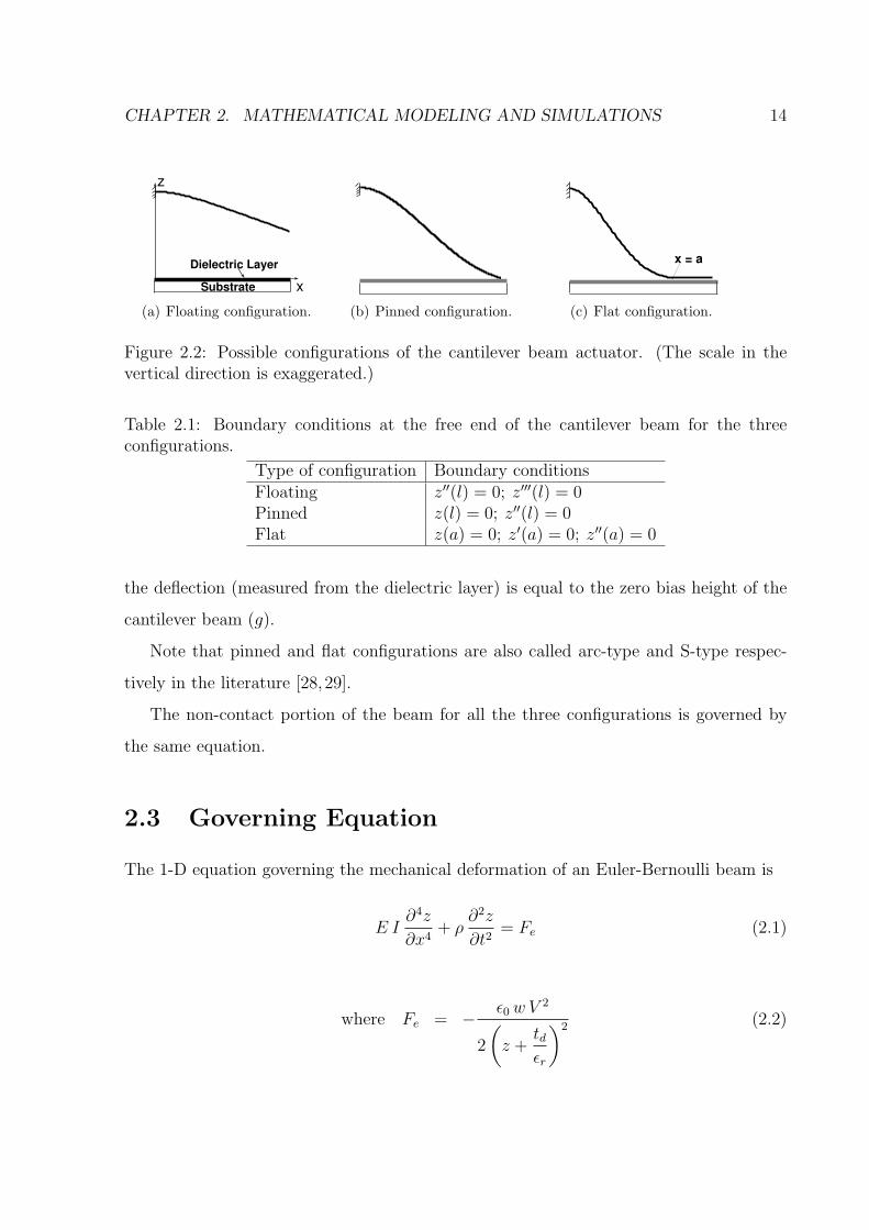
1. Floating Configuration: The cantilever beam has no contact with the dielectric layer
and is illustrated in Fig. 2.2(a). The bending moment and shear force at the free
12
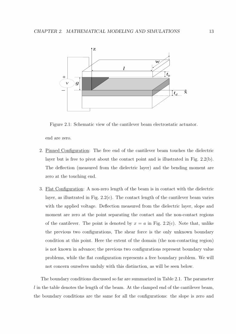
CHAPTER 2. MATHEMATICAL MODELING AND SIMULATIONS 13
x
z
td
l
w
g
tb+
_V
Figure 2.1: Schematic view of the cantilever beam electrostatic actuator.
end are zero.
2. Pinned Configuration: The free end of the cantilever beam touches the dielectric
layer but is free to pivot about the contact point and is illustrated in Fig. 2.2(b).
The deflection (measured from the dielectric layer) and the bending moment are
zero at the touching end.
3. Flat Configuration: A non-zero length of the beam is in contact with the dielectric
layer, as illustrated in Fig. 2.2(c). The contact length of the cantilever beam varies
with the applied voltage. Deflection measured from the dielectric layer, slope and
moment are zero at the point separating the contact and the non-contact regions
of the cantilever. The point is denoted by x = a in Fig. 2.2(c). Note that, unlike
the previous two configurations, The shear force is the only unknown boundary
condition at this point. Here the extent of the domain (the non-contacting region)
is not known in advance; the previous two configurations represent boundary value
problems, while the flat configuration represents a free boundary problem. We will
not concern ourselves unduly with this distinction, as will be seen below.
The boundary conditions discussed so far are summarized in Table 2.1. The parameter
l in the table denotes the length of the beam. At the clamped end of the cantilever beam,
the boundary conditions are the same for all the configurations: the slope is zero and
CHAPTER 2. MATHEMATICAL MODELING AND SIMULATIONS 14
Dielectric Layer
Substrate
z
x
(a) Floating configuration. (b) Pinned configuration.
x = a
(c) Flat configuration.
Figure 2.2: Possible configurations of the cantilever beam actuator. (The scale in thevertical direction is exaggerated.)
Table 2.1: Boundary conditions at the free end of the cantilever beam for the threeconfigurations.
Type of configuration Boundary conditionsFloating z′′(l) = 0; z′′′(l) = 0Pinned z(l) = 0; z′′(l) = 0Flat z(a) = 0; z′(a) = 0; z′′(a) = 0
the deflection (measured from the dielectric layer) is equal to the zero bias height of the
cantilever beam (g).
Note that pinned and flat configurations are also called arc-type and S-type respec-
tively in the literature [28,29].
The non-contact portion of the beam for all the three configurations is governed by
the same equation.
2.3 Governing Equation
The 1-D equation governing the mechanical deformation of an Euler-Bernoulli beam is
E I∂4z
∂x4+ ρ
∂2z
∂t2= Fe (2.1)
where Fe = − ε0w V2
2
(z +
tdεr
)2 (2.2)

CHAPTER 2. MATHEMATICAL MODELING AND SIMULATIONS 15
Table 2.2: Description of the parameters in the governing equation.
Parameter Descriptionl Beam lengthw Beam widthtb Beam thicknesstd Dielectric layer thicknessρ Mass per unit length of the beamg Zero bias height of the cantilever beamA Beam cross-sectional area (= w tb)
I Moment of inertia of the beam cross-section
(=w t3b12
)E Young’s modulus of the beam materialε0 Permittivity of free spaceεr Relative permittivity of the dielectric or dielectric constantV Applied voltage
Fe is the electrical force per unit length. The derivation for Fe is along the lines of
derivation in section 1.2.1 except that there is a change in the sign convention of coordinate
axes. The variables x and z in the above equations denote the position along the length
and the lateral deflection of the beam respectively; and t is time. Effects like step-
ups, stress-stiffening and softened contact surfaces are not included in this model. The
parameters in the governing equation are described in Table 2.2.
The common practice [7] of using a fringing field correction such as 0.65 (z+td/εr)w
is
not adopted here. In the post-pull-in regime, the cantilever beam has portions very close
to the dielectric, where the fringing field is small. Further, neglecting the fringing field
makes the analysis simpler and provides useful insights. Finally, calculations including
the fringing field, though slightly complex, could if necessary be carried out using the
approach adopted in this thesis.
2.4 Normalized Equation
The length quantities x and z (refer to Fig. 2.1) are normalized with respect to the
length and zero bias height of the beam. Time t is normalized with respect to a constant
T , defined in such a way that the parameter ρ in Eq. 2.1 becomes unity. All the further

CHAPTER 2. MATHEMATICAL MODELING AND SIMULATIONS 16
analysis is carried out on the normalized equation and the results thus obtained are finally
scaled to the actual parameters. The normalized quantities are as follows.
x =x
l(2.3)
z =z
g(2.4)
t =t
T(2.5)
where T =
√ρ l4
E I(2.6)
Two other non-dimensional quantities are defined as follows.
V =
√ε0w l4
2E I g3V , (2.7)
h =tdg εr
. (2.8)
The governing equation becomes
∂4z
∂x4+∂2z
∂t2= − V 2
(z + h)2 (2.9)
For static analysis, there is no time dependence and the equation reduces to
d4z
dx4= − V 2
(z + h)2 (2.10)
The hats in the normalized equation are dropped for convenience in the following analysis.
The following sections present the details simulation techniques.

CHAPTER 2. MATHEMATICAL MODELING AND SIMULATIONS 17
2.5 Modal Expansion Method
2.5.1 Modal Expansion Method in General
The coupled electro-mechanical equation of the electrostatically actuated beams (Eq. 2.10)
can be solved using modal expansion method. The deflection of the beam is expressed as a
superposition of its modes. The modes are constructed in such a way that the mechanical
force per unit length on any mode is proportional to the mode deflection. So, if the force
per unit length on a mode is known, the corresponding deflection can be calculated by
multiplying it with the suitable proportionality constant and vice versa. Mechanical force
per unit length (Fmech) is the fourth order derivative of beam deflection z. The fourth
order derivatives of sin, cos, sinh and cosh functions are proportional to the respective
functions themselves. So, each mode is constructed as a combination of these functions.
Let
ψj(x) = jth mode of the beam.
z(x) = Beam deflection.
z0(x) = Initial position of the beam.
w(x) = Beam deflection from the initial position.
z(x) can be expressed as
z(x) = z0(x) + w(x). (2.11)
ψj(x) is expressed as
ψj(x) = B1j sin(λj x) +B2j cos(λj x) +B3j sinh(λj x) +B4j cosh(λj x). (2.12)
The values of B1j, B2j, B3j,B4j and λj are evaluated from the boundary conditions. w(x)
is expressed as
w(x) =N∑j=1
aj ψj(x). (2.13)
⇒ z(x) = z0(x) +N∑j=1
aj ψj(x) (2.14)

CHAPTER 2. MATHEMATICAL MODELING AND SIMULATIONS 18
where aj is the participation factor associated with the jth mode and is called modal
amplitude of jth mode.
When the applied voltage is zero,
z(x) = z0(x).
Then the mechanical force per unit length should also be zero.
⇒ Fmech =d4z
dx4=d4z0
dx4= 0
⇒ d4z0
dx4= 0 (2.15)
So, mechanical force per unit length can be expressed as
Fmech =d4z
dx4=d4w
dx4=
N∑j=1
λ4j aj ψj(x). (2.16)
The boundary conditions at the clamped end are same for all the configurations and are
z(0) = 1⇒ ψj(0) = 0
z′(0) = 0⇒ ψ′j(0) = 0.
From these boundary conditions and by taking B4j = 1, B3j = Bj, Eq. 2.12 reduces to
the following form.
ψj(x) = cosh (λj x)− cos (λj x)−Bj (sinh (λj x)− sin (λj x)) (2.17)

CHAPTER 2. MATHEMATICAL MODELING AND SIMULATIONS 19
Bj and λj are computed from the boundary conditions at the free end of the cantilever
beam. The derivatives of ψj w.r.t. x are
ψ′j(x) = λj (sinh (λj x) + sin (λj x)−Bj (cosh (λj x)− cos (λj x))) (2.18)
ψ′′j (x) = λ2j (cosh (λj x) + cos (λj x)−Bj (sinh (λj x) + sin (λj x))) (2.19)
ψ′′′j (x) = λ3j (sinh (λj x)− sin (λj x)−Bj (cosh (λj x) + cos (λj x))) (2.20)
ψ′′′′j (x) = λ4j (cosh (λj x)− cos (λj x)−Bj (sinh (λj x)− sin (λj x))) = λ4
jψj(x). (2.21)
The modes possess the following orthogonality relation:
1∫0
ψi(x)ψj(x) dx =
1 if i = j
0 Otherwise(2.22)
Computation of Modal Amplitudes
The modal amplitudes are computed using the orthogonality relation in Eq. 2.22. The
procedure is as follows:
Multiplying Eq. 2.16, with ψi(x) on both sides and integrating from 0 to 1 w.r.t x,
1∫0
Fmech ψi(x) dx =
1∫0
N∑j=1
aj ψj(x)ψi(x) dx.
Interchanging summation and integration on the right hand side of the above equation,
1∫0
Fmech ψi(x) dx =N∑j=1
1∫0
ajψj(x)ψi(x) dx
⇒1∫
0
Fmech ψi(x) dx =N∑
j=1j 6=i
aj
1∫0
ψj(x)ψi(x) dx+ ai
1∫0
ψ2i (x) dx.
CHAPTER 2. MATHEMATICAL MODELING AND SIMULATIONS 20
From the orthogonality relation in Eq. 2.22, above equation reduces to to the following
form.
ai =
1∫0
Fmech ψi(x) dx (2.23)
In this equation, i is varied from 1 to N and the corresponding modal amplitudes are
computed.
The boundary conditions of the configurations are discussed in section 2.2 and are
summarized in Table 2.1. The necessary equations for solving the floating and pinned
configurations are derived in the following subsections.
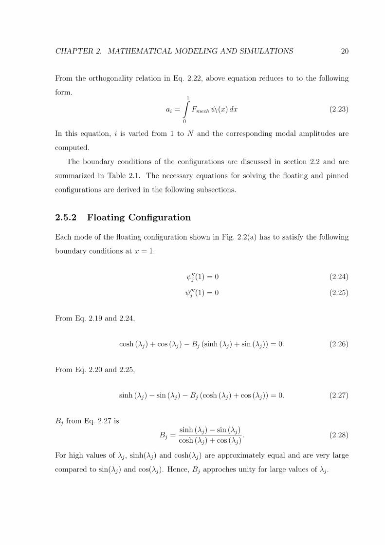
2.5.2 Floating Configuration
Each mode of the floating configuration shown in Fig. 2.2(a) has to satisfy the following
boundary conditions at x = 1.
ψ′′j (1) = 0 (2.24)
ψ′′′j (1) = 0 (2.25)
From Eq. 2.19 and 2.24,
cosh (λj) + cos (λj)−Bj (sinh (λj) + sin (λj)) = 0. (2.26)
From Eq. 2.20 and 2.25,
sinh (λj)− sin (λj)−Bj (cosh (λj) + cos (λj)) = 0. (2.27)
Bj from Eq. 2.27 is
Bj =sinh (λj)− sin (λj)
cosh (λj) + cos (λj). (2.28)
For high values of λj, sinh(λj) and cosh(λj) are approximately equal and are very large
compared to sin(λj) and cos(λj). Hence, Bj approches unity for large values of λj.

CHAPTER 2. MATHEMATICAL MODELING AND SIMULATIONS 21
Table 2.3: Roots and coefficient values of various modes of the floating configuration.
Modes of Vibration (j) λj Bj
1 1.8751 0.734092 4.6941 1.018473 7.8548 0.999224 10.9955 1 + 3.35× 10⁻⁵
5 14.1372 16 17.2788 1
Substituting Bj in Eq. 2.26,
cosh (λj) + cos (λj)− sinh (λj)− sin (λj)
cosh (λj) + cos (λj)(sinh (λj) + sin (λj)) = 0
⇒ cosh2 (λj) + cos2 (λj) + 2 cosh (λj) cos (λj)− sinh2 (λj) + cos2 (λj) = 0
⇒ 1 + cosh (λj) cos (λj) = 0 (2.29)
Eq. 2.29 is the characteristic equation of the floating configuration. The roots of the
characteristic equation can be determined using numerical methods like Newton-Raphson
method. Table 2.3 summarizes the roots (λj) and the coefficient values (Bj) of the first
six modes of operation.
Deflection of the beam
The initial position of the floating configuration is
z0(x) = 1
⇒ z(x) = 1 +N∑j=1
ajψj(x) (2.30)
CHAPTER 2. MATHEMATICAL MODELING AND SIMULATIONS 22
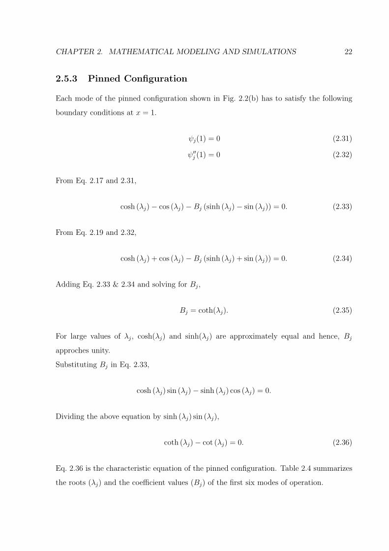
2.5.3 Pinned Configuration
Each mode of the pinned configuration shown in Fig. 2.2(b) has to satisfy the following
boundary conditions at x = 1.
ψj(1) = 0 (2.31)
ψ′′j (1) = 0 (2.32)
From Eq. 2.17 and 2.31,
cosh (λj)− cos (λj)−Bj (sinh (λj)− sin (λj)) = 0. (2.33)
From Eq. 2.19 and 2.32,
cosh (λj) + cos (λj)−Bj (sinh (λj) + sin (λj)) = 0. (2.34)
Adding Eq. 2.33 & 2.34 and solving for Bj,
Bj = coth(λj). (2.35)
For large values of λj, cosh(λj) and sinh(λj) are approximately equal and hence, Bj
approches unity.
Substituting Bj in Eq. 2.33,
cosh (λj) sin (λj)− sinh (λj) cos (λj) = 0.
Dividing the above equation by sinh (λj) sin (λj),
coth (λj)− cot (λj) = 0. (2.36)
Eq. 2.36 is the characteristic equation of the pinned configuration. Table 2.4 summarizes
the roots (λj) and the coefficient values (Bj) of the first six modes of operation.

CHAPTER 2. MATHEMATICAL MODELING AND SIMULATIONS 23
Table 2.4: Roots and coefficient values of various modes of the pinned configuration.
Modes of Vibration (j) λj Bj
1 3.9266 1 + 7.8× 10⁻⁴
2 7.0686 13 10.2102 14 13.3518 15 16.4934 16 19.6350 1
Deflection of the beam
Let the initial position of the beam in pinned configuration be expressed as a polynomial
in x as follows.
z0(x) = a0 + a1x+ a2x2 + a3x
3 + a4x4 + · · ·+ anx
n (2.37)
When no voltage is applied, from Eq. 2.15 and 2.37,
a4 = a5 = · · · = an = 0
⇒ z0(x) = a0 + a1x+ a2x2 + a3x
3. (2.38)
The boundary conditions at the clamped end are,
z0(0) = 1⇒ ao = 1
z′0(0) = 0⇒ a1 = 0
⇒ z0(x) = 1 + a2x2 + a3x
3. (2.39)
The boundary conditions at the pinned end are,
z0(1) = 0⇒ 1 + a2 + a3 = 0
z′′0 (1) = 0⇒ a2 + 3a3 = 0

CHAPTER 2. MATHEMATICAL MODELING AND SIMULATIONS 24
Table 2.5: Characteristic equations, coefficient values and Initial position of the beam forvarious configurations.
Type of configuration Characteristic Equation Coefficient value z0(x)
Floating 1 + cosh (λj) cos (λj) = 0sinh(λj)−sin(λj)
cosh(λj)+cos(λj)1
Pinned coth (λj)− cot (λj) = 0 coth(λj) 1− 32x2 + 1
2x
Solving the above equations, we get
z0(x) = 1− 3
2x2 +
1
2x3.
⇒ z(x) =
(1− 3
2x2 +
1
2x3
)+
N∑j=1
ajψj(x) (2.40)
Table 2.5 summarizes the characteristic equations, Bj values and initial positions of the
beam for the floating and pinned configurations.
2.5.4 Procedure to Solve the Coupled Equation
The iterative procedure to solve the coupled electro-mechanical equation using modal ex-
pansion method is described here.
Input: The dimensions and material properties of the beam, dielectric constant, dielectric
layer thickness, zero bias height and the applied voltage are given as inputs to the method.
Initialization: The deflection of the beam from the initial position i.e., w(x) is initialized
to zero. In other words, all the modal amplitudes are initialized to zero.
The non-dimensional quantities in the normalized equation are computed and the follow-
ing steps are followed.
Step 1: Compute Electrostatic Force
Electrostatic force per unit length is computed from the relation
Fe = − V 2
(z + h)2
Step 2: Find the Modal Expansion of the Force
All the modal amplitudes (ai values) of the force are computed from Eq. 2.23.
CHAPTER 2. MATHEMATICAL MODELING AND SIMULATIONS 25
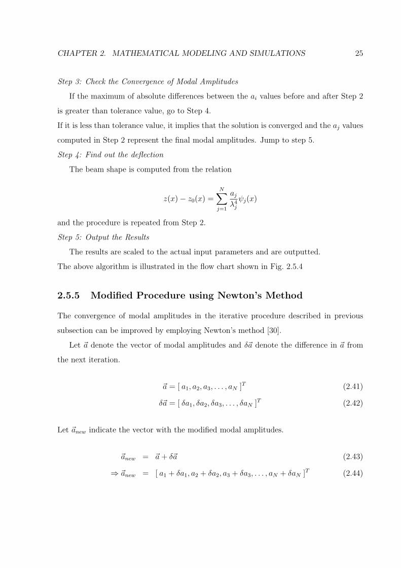
Step 3: Check the Convergence of Modal Amplitudes
If the maximum of absolute differences between the ai values before and after Step 2
is greater than tolerance value, go to Step 4.
If it is less than tolerance value, it implies that the solution is converged and the aj values
computed in Step 2 represent the final modal amplitudes. Jump to step 5.
Step 4: Find out the deflection
The beam shape is computed from the relation
z(x)− z0(x) =N∑j=1
ajλ4j
ψj(x)
and the procedure is repeated from Step 2.
Step 5: Output the Results
The results are scaled to the actual input parameters and are outputted.
The above algorithm is illustrated in the flow chart shown in Fig. 2.5.4
2.5.5 Modified Procedure using Newton’s Method
The convergence of modal amplitudes in the iterative procedure described in previous
subsection can be improved by employing Newton’s method [30].
Let ~a denote the vector of modal amplitudes and δ~a denote the difference in ~a from
the next iteration.
~a = [ a1, a2, a3, . . . , aN ]T (2.41)
δ~a = [ δa1, δa2, δa3, . . . , δaN ]T (2.42)
Let ~anew indicate the vector with the modified modal amplitudes.
~anew = ~a+ δ~a (2.43)
⇒ ~anew = [ a1 + δa1, a2 + δa2, a3 + δa3, . . . , aN + δaN ]T (2.44)

CHAPTER 2. MATHEMATICAL MODELING AND SIMULATIONS 26
START
INPUT l, w, tb, td, 0r , g, E, V
INITIALISE DEFLECTION=0
i.e., aj = 0 for all j =1 to N & CALCULATE THE NON-
DIMENSIONAL QUANTITIES
CALCULATE ELECTROSTATIC FORCE
2
2
)( hz
VFe
��
FIND MODAL EXPANSION OF FORCE
)()(4
1
xFxa ejj
n
j
j ¦
\O
ARE NEW aj
VALUES CLOSE TO PREVIOUS VALUES?
STOP
YES
NO
FIND DEFLECTION AS
)()()(1
0 xaxzxz j
n
j
j\¦
�
Figure 2.3: Flow chart for Modal Expansion Method.

CHAPTER 2. MATHEMATICAL MODELING AND SIMULATIONS 27
If ~anew represents the exact modal amplitudes,
n∑j=1
(~anew)j λ4jψj(x) = − V 2
(z(x) + h)2 (2.45)
where (~anew)j represents the jth component of ~anew.
Multiplying Eq. 2.45 with ψi(x) on both sides and integrating from 0 to 1 w.r.t. x,
1∫0
N∑j=1
(~anew)j λ4jψj(x)ψi(x) dx = −
1∫0
V 2
(z(x) + h)2ψi(x) dx.
The variable i in the above equation can have any value from 0 to N . Interchanging inte-
gration and summation on the left hand side of the above equation and using orthogonal
relation of modes specified in Eq. 2.22, the above equation reduces to the following form.
(~anew)i λ4i = −
1∫0
V 2
(z(x) + h)2ψi(x) dx (2.46)
Let
Fi (~anew) = Fi (~a+ δ~a) = (~anew)i λ4i +
1∫0
V 2
(z(x) + h)2ψi(x) dx = 0 (2.47)
For i = 1 to N , we get N such equations. Let
~F (~anew) = [ F1 (~anew) , F2 (~anew) , F3 (~anew) , . . . , FN (~anew) ]T . (2.48)
Writing Eq. 2.47 in vector form taking all values of i,
~F (~a+ δ~a) = 0⇒ ~F (~a) + J δ~a = 0. (2.49)
where J is the Jacobian matrix defined as
Ji,j =∂Fi∂aj
. (2.50)

CHAPTER 2. MATHEMATICAL MODELING AND SIMULATIONS 28
From Eq. 2.49,
δ~a = −J−1 ~F (~a) (2.51)
where
Fi (~a) = aiλ4i +
1∫0
V 2
(z(x) + h)2ψi(x) dx. (2.52)
Let
fi = − V 2
(z(x) + h)2 ψi(x). (2.53)
⇒ ∂fi∂aj
=∂fi∂z
∂z
∂aj(2.54)
Substituting Eq. 2.53 in Eq. 2.52,
Fi (~a) = ai λ4i −
1∫0
fi dx. (2.55)
From Eq. 2.53,∂fi∂z
=2V 2
(z(x) + h)3ψi(x).
From Eq. 2.14,
∂z
∂aj= ψj(x).
⇒ ∂fi∂aj
=2V 2
(z(x) + h)3ψi(x)ψj(x) (2.56)
From Eq. 2.55 and 2.56,
∂Fi∂aj
=
λ4i −
1∫0
∂fi
∂ajdx if i = j
−1∫0
∂fi
∂ajdx Otherwise.
(2.57)

CHAPTER 2. MATHEMATICAL MODELING AND SIMULATIONS 29
From Eq. 2.50, 2.56 and 2.57,
Ji,j =
λ4i −
1∫0
2V 2
(z(x)+h)3ψ2i (x) dx if i = j
−1∫0
2V 2
(z(x)+h)3ψi(x)ψj(x) dx Otherwise.
(2.58)
From the above equation, it is evident that
∂Fi (~a)
∂aj=∂Fj (~a)
∂ai⇒ Ji,j = Jj,i. (2.59)
Hence, Jacobian in this case is a symmetric matrix.
Algorithm
The input and the initialization part are similar to the general method discussed in the
previous subsection. The steps are as follows:
Step 1: Compute Fi (~a) from Eq. 2.52, for all values of i from 1 to N
Step 2: Compute Jacobian matrix J from Eq. 2.58, and δ~a from Eq. 2.51.
Step 3: If max(abs(δ~a)) < tolerance value, the solution is converged and jump to Step 5.
else, go to Step 4
Step 4: ~anew is computed from Eq. 2.43. ~a is replaced with ~anew and the the procedure
repeated from Step 1.
Step 5: The results are scaled to the actual input parameters and are outputted
The above procedure is illustrated in detail in the flow chart shown in Fig. 2.5.5
Finite difference scheme is developed in the following section to solve all the three
configurations.
CHAPTER 2. MATHEMATICAL MODELING AND SIMULATIONS 30
START
INPUT l, w, tb, td, 0r ,g, E, V
INITIALISE DEFLECTION = 0
i.e., ai = 0 for all i =1 to N & CALCULATE THE NON-
DIMENSIONAL QUANTITIES
CALCULATE THE FOLLOWING FUNCTION FOR i = 1 TO N
³ ��
1
0))((
4 )()( 2
2dxxaaF ihxz
Viii \O
Is
max ( abs ( aG ) ) < TOL?
STOP
YES
NO
aaa G�
CALCULATE JACOBIAN ( J ) FOR ABOVE N FUNCTIONS w.r.t. a .
& CALCULATE FJa 1�� G
SCALE THE RESULTS TO I/P PARAMETERS
Figure 2.4: Flow chart for Modal Expansion Method that employs Newton’s Method.

CHAPTER 2. MATHEMATICAL MODELING AND SIMULATIONS 31
2.6 Finite Difference Approximation
2.6.1 Method
In finite difference (F.D.) scheme, the derivatives are replaced by finite difference approx-
imations and the resulting system of algebraic equations is solved. Where the boundary
conditions involve derivatives, we introduce suitable fictitious points beyond the physical
boundaries.
Specifically, a five point central difference scheme is implemented because a fourth
order derivative is involved. Two fictitious points are introduced on each side of the
non-contact length of the cantilever beam.
The governing Eq. 2.10 to be solved can be wriiten as,
d4z
dx4+
V 2
(z + h)2 = 0. (2.60)
The non-contact length of the cantilever beam is divided into a uniform grid of N points
along the x-axis with a step size of ∆x. These points are denoted by x1, x2, · · · xN−1, xN .
Let zi denote the beam deflection at x = xi, i = 1, 2, · · · , N . Let the fictitious points be
denoted by z0, z−1 on the left side and zN+1, zN+2 on the right side of the non-contact
length with the same step size, ∆x. Hence, totally N + 4 points are considered along the
x-axis.
Finite diiference approximations are derived as follows. From Taylor’s series expansion,
z values at xi+1, xi−1, xi+2, xi−2 can be written as,
zi+1 = zi + (∆x) z′i +(∆x)2
2z′′i +
(∆x)3
6z′′′i +
(∆x)4
24z′′′′i (2.61)
zi−1 = zi − (∆x) z′i +(∆x)2
2z′′i −
(∆x)3
6z′′′i +
(∆x)4
24z′′′′i (2.62)
zi+2 = zi + 2 (∆x) z′i +4 (∆x)2
2z′′i +
8 (∆x)3
6z′′′i +
16 (∆x)4
24z′′′′i (2.63)
zi−2 = zi − 2 (∆x) z′i +4 (∆x)2
2z′′i −
8 (∆x)3
6z′′′i +
16 (∆x)4
24z′′′′i . (2.64)
The finite difference approximations of the derivatives are computed by solving the above

CHAPTER 2. MATHEMATICAL MODELING AND SIMULATIONS 32
equations and are as follows.
z′i =zi−2 − 8 zi−1 + 8 zi+1 − zi+2
12 (∆x)(2.65)
z′′i =−zi−2 + 16 zi−1 − 30 zi + 16 zi+1 − zi+2
12 (∆x)2 (2.66)
z′′′i =−zi−2 + 2 zi−1 − 2 zi+1 + zi+2
2 (∆x)3 (2.67)
z′′′′i =zi−2 − 4 zi−1 + 6 zi − 4 zi+1 + zi+2
(∆x)4 (2.68)
for i = 1, 2, · · ·N .
The governing Eq. 2.60 in terms of finite differences is
zi−2 − 4 zi−1 + 6 zi − 4 zi+1 + zi+2 +(∆x)4 V 2
(zi + h)2 = 0. (2.69)
The solution procedure to solve the system of nonlinear algebraic equations is described
below. Newton’s method [30] is used to improve the convergence of the solution scheme.
Let z = [ z−1, z0, z1, . . . zN , zN+1, zN+2 ]T (2.70)
fi(z) = zi−2 − 4 zi−1 + 6 zi − 4 zi+1 + zi+2 +(∆x)4 V 2
(zi + h)2, for i = 1to N. (2.71)
Let F (z) be defined as
F (z) = [ f1(z), f2(z), . . . fN(z), fN+1(z), fN+2(z), fN+3(z), fN+4(z) ]T . (2.72)
f1 to fN are computed from Eq. 2.71 and fN+1 to fN+4 are computed from the boundary
conditions of the corresponding configurations as described later.
Let δz = [ δz−1, δz0, δz1, . . . δzN+2 ]T (2.73)
be the correction vector such that F (z + δz) = 0.
⇒ F (z) + J δz = 0 (2.74)

CHAPTER 2. MATHEMATICAL MODELING AND SIMULATIONS 33
where J is the Jacobian matrix with,
Ji, j =∂fi∂zj
, for i = 1 to N + 4, j = −1 to N + 2. (2.75)
From Eq. 2.74,
δz = −J−1 F (z). (2.76)
The non-zero elements of Jacobian matrix for i = 1 to N can be computed from the
derivatives Eq. 2.71 and are as follows:
Ji, i−2 = Ji, i+2 = 1 ;
Ji, i−1 = Ji, i+1 = −4 ;
Ji, i = 6− 2 (∆x)4 V 2
(zi + h)3. (2.77)
The elements of J and F for i = N+1 to N+4 are computed from boundary conditions
and hence, they are configuration specific. These details along with the solution procedure
are presented in the following subsections.
2.6.2 Floating Configuration
At the clamped end of the cantilever beam, deflection is 1 and slope is 0. Replacing the
derivatives in the boundary conditions by finite differences and considering them as fN+1
and fN+2,
fN+1 = z1 − 1 (2.78)
fN+2 = z−1 − 8 z0 + 8 z2 − z3 (2.79)

CHAPTER 2. MATHEMATICAL MODELING AND SIMULATIONS 34
At the free end, bending moment (z′′) and shear force (z′′′) are zero. Replacing these
derivatives by finite differences, we get the following equations.
fN+3 = −zN−2 + 16 zN−1 − 30 zN + 16zN+1 − zN+2 (2.80)
fN+4 = −zN−2 + 2 zN−1 − 2 zN+1 + zN+2 (2.81)
The non-zero values of Jacobian matrix for these boundary conditions are
JN+1, 1 = 1 ; (2.82)
JN+2,−1 = 1 ; JN+2, 0 = −8 ; JN+2, 2 = 8 ; JN+2, 3 = −1 ; (2.83)
JN+3, N−2 = JN+3,N+2 = −1 ; JN+3, N−1 = JN+3,N+1 = 16 ; JN+3, N) = −30 ; (2.84)
JN+4, N−2 = −1 ; JN+4, N−1 = 2 ; JN+4, N+1 = −2 ; JN+4, N+2 = 1 ; (2.85)
In this configuration, the non-contact length is known and is equal to 1 for the nor-
malized case. Hence, z value at N+4 points are the only unknowns. The system of N+4
nonlinear equations (Eq. 2.72) is solved through an iterative procedure and z values are
computed. The procedure is outlined in the flow chart shown in Fig. 2.6.2.
2.6.3 Pinned Configuration
The boundary conditions at the clamped end are same as floating configuration. fN+1
and fN+2 are same as floating equation and are shown in Eq. 2.78 and 2.79. Hence, the
corresponding Jacobian matrix values are also same as Eq. 2.82 and 2.83.
At the touching end, deflection (z) and bending moment (z′′) are zero and in terms of
finite differences, they are expressed as follows.
fN+3 = zN (2.86)
fN+4 = −zN−2 + 16 zN−1 − 30 zN + 16zN+1 − zN+2 (2.87)

CHAPTER 2. MATHEMATICAL MODELING AND SIMULATIONS 35
Start
Input l, w, tb, td, 0r ,g, E, V
Initialize deflection & calculate the non-dimensional
quantities
Compute F(z) and Jacobian (J)
Yes
Is max (abs( zG ))
< TOL?
Stop
zzz G�
Compute )(1 zFJz �� G
Scale the results to i/p parameters
No
Figure 2.5: Flow chart for Finite difference approximation of floating and pinned config-urations.

CHAPTER 2. MATHEMATICAL MODELING AND SIMULATIONS 36
The corresponding Jacobian matrix elements are,
JN+3, N = 1 ; (2.88)
JN+4, N−2 = JN+4,N+2 = −1 ; JN+4, N−1 = JN+4,N+1 = 16 ; JN+4, N) = −30 ; (2.89)
The non-contact length, number of unknowns and solution procedure are exactly identical
to the floating configuration as outlined in the flow chart shown in Fig. 2.6.2.
2.6.4 Flat Configuration
In this configuration, the non-contact length varies with the applied voltage and hence,
is an unknown quantity. This problem turns out to be a free boundary problem. The
solution procedure has a minor adition to the previous two configurations. The bound-
ary conditions at the clamped end are same as other configurations. At the other end,
deflection (z), slope (z′) and bending moment (z′′) are zero. Hence, unlike the other two
configurations, 5 boundary conditions are known in the flat configuration.
For the flat configuration, any one solution determines all other solutions by a scaling
law discussed in the following section. The procedure to find one solution, for which we
assume the non-contacting length is unity, is as follows. V is initialized with an arbitrary
value. The corresponding value of z is computed using the three boundary conditions at
the flat end (at zN) and zero slope condition at the fixed end (at z1). In other words,
the boundary condition that z1 = 1 is initially ignored. With V given, this is enough
to determine the solution. The computed value of z1 should be unity. The chosen V is
iteratively modified to match this condition. Once this V is found, all other flat solutions
for the same h can be found by scaling as discussed in the following section.
CHAPTER 2. MATHEMATICAL MODELING AND SIMULATIONS 37
The function values considered from the boundary conditions are as follows.
fN+1 = z−1 − 8 z0 + 8 z2 − z3 (2.90)
fN+2 = zN (2.91)
fN+3 = zN−2 − 8 zN−1 + 8 zN+1 − zN+2 (2.92)
fN+4 = −zN−2 + 16 zN−1 − 30 zN + 16zN+1 − zN+2 (2.93)
The non-zero elements of the Jacobian matrix associated with these functions are
JN+1,−1 = 1 ; JN+1, 0 = −8 ; JN+1, 2 = 8 ; JN+1, 3 = −1 ; (2.94)
JN+2, N = 1 ; (2.95)
JN+3, N−2 = 1 ; JN+3, N−1 = −8 ; JN+3, N+1 = 8 ; JN+3, N+2 = −1 ; (2.96)
JN+4, N−2 = JN+4,N+2 = −1 ; JN+4, N−1 = JN+4,N+1 = 16 ; JN+4, N) = −30 ; (2.97)
2.7 Scaling Law in the Flat Configuration
In the flat regime, a scaling law is found. Due to this scaling, if the solution is computed
at one voltage, solutions at all other voltages can be found out with out actually solving
the governing equation again. The solution computed at one voltage can be scaled ap-
propriately to get the solutions at all other voltages. The scaling law is deduced from the
following analysis.
Let
ζ = x√V (2.98)
The governing Eq.2.10, in terms of ζ is
d4z
dζ4=
−1
(z + h)2(2.99)

CHAPTER 2. MATHEMATICAL MODELING AND SIMULATIONS 38
Let the ζ value at x = a be denoted by ζ0. The boundary conditions expressed in terms
of ζ and are
z (ζ = 0) = 1 and z′ (ζ = 0) = 0
z (ζ = ζ0) = z′ (ζ = ζ0) = z′′ (ζ = ζ0) = 0 (2.100)
It is evident from Eq. 2.99 and 2.100 that neither the governing equation nor the boundary
conditions are dependent on the applied voltage. The values of ζ0, z (ζ) for a given voltage
can be computed from the numerical procedure described previously and they are constant
for a given value of h. Let α be the non-contact length of the beam for an applied voltage
of V . As ζ0 is constant for a given h,
α√V = ζ0 = constant (2.101)
Hence, ζ0 computed at any voltage determines the constant value and can be subsequently
used to compute the non-contact lengths at all other voltages. Similarly, z value computed
at one voltage can be used to compute the z values at all other voltages. Another point
to be noted is that this scaling law is applicable even to the models [7, 23] that account
for fringing field.
2.8 Discussion and Conclusions
Cantilever beam MEMS electrostatic actuators with an intermediate dielectric layer or
modeled over the entire operational range. Three possible static configurations are iden-
tified in the operational range: floating, pinned and flat configurations. The non-contact
length in all the configurations is governed by the same equation but they differ in the
boundary conditions. Modal expansion method and finite difference method are devel-
oped to perform the simulations. A scaling law is found in the flat configuration. Using
this scaling, solution computed at one voltage is aprropriately scaled to get the solutions
at all other voltages in the flat configuration. The governing Eq. 2.10 along with the
boundary conditions constitutes a nonlinear boundary value problem for the floating and

CHAPTER 2. MATHEMATICAL MODELING AND SIMULATIONS 39
pinned configurations and a nonlinear free boundary problem for the flat configuration.
The free boundary problem is transformed into an iterative boundary value problem by
using the additionally available boundary condition.

Chapter 3
Effects of Dielectric Layer
3.1 Introduction
The governing Eq. 2.10 has only two parameters V and h. h is proportional to the
dielectric thickness for a given zero bias height and dielectric constant. Similarly, V is
proportional to the applied voltage. The effects of dielectric layer thickness are studied
by finding out the solutions for fixed h and varying V , for a range of values of h.
The following section gives details regarding voltage limits of the three possible con-
figurations of the beam.
3.2 Normalized Voltage (V ) Limits of Configurations
1. Floating Configuration: The lower limit (V minfloat) is, trivially, zero. The upper limit
(V maxfloat) is decided either by disappearance of solutions via a so-called turning point
(for small h, as discussed later), or (for large h) contact with the dielectric layer.
Beyond this upper limit, the actuator switches to the pinned or flat configuration.
2. Pinned Configuration: The end of the beam can, in principle, always be held pinned
(say, by an external agent) against the dielectric layer by a suitable additional
vertical force at the end point. If that force needs to act downwards, then such
a pinned solution is physically unfeasible because when we remove that force the
40
CHAPTER 3. EFFECTS OF DIELECTRIC LAYER 41
end point moves up. Upward acting forces are feasible because when we remove
that force the end point tends to move down and presses against the dielectric layer
which, through mechanical contact, can apply an upward force.
The lower limit (V minpin ) is therefore voltage at which shear force at the contacting end
of the cantilever beam becomes zero (and the boundary conditions of the pinned
configuration are also satisfied). Below V minpin , the dielectric layer would have to
mechanically pull down on the free end: since it cannot do so, the actuator is in the
floating configuration. The upper limit (V maxpin ) is decided either by disappearance
of solutions via a so-called turning point (for small h, as discussed later), or (for
large h) extended contact with the dielectric layer (zero slope at the end). Beyond
this upper limit, the actuator switches to the flat configuration. The transition at
(V maxpin ) has not been elucidated in the literature, and is one of post-pull-in insights
offered in this thesis.
3. Flat configuration: The lower limit (V minflat ) is that at which the non-contacting length
of the beam equals the total length of the beam. There is no upper V limit for the
flat configuration. The non-contacting length approaches zero as V →∞.
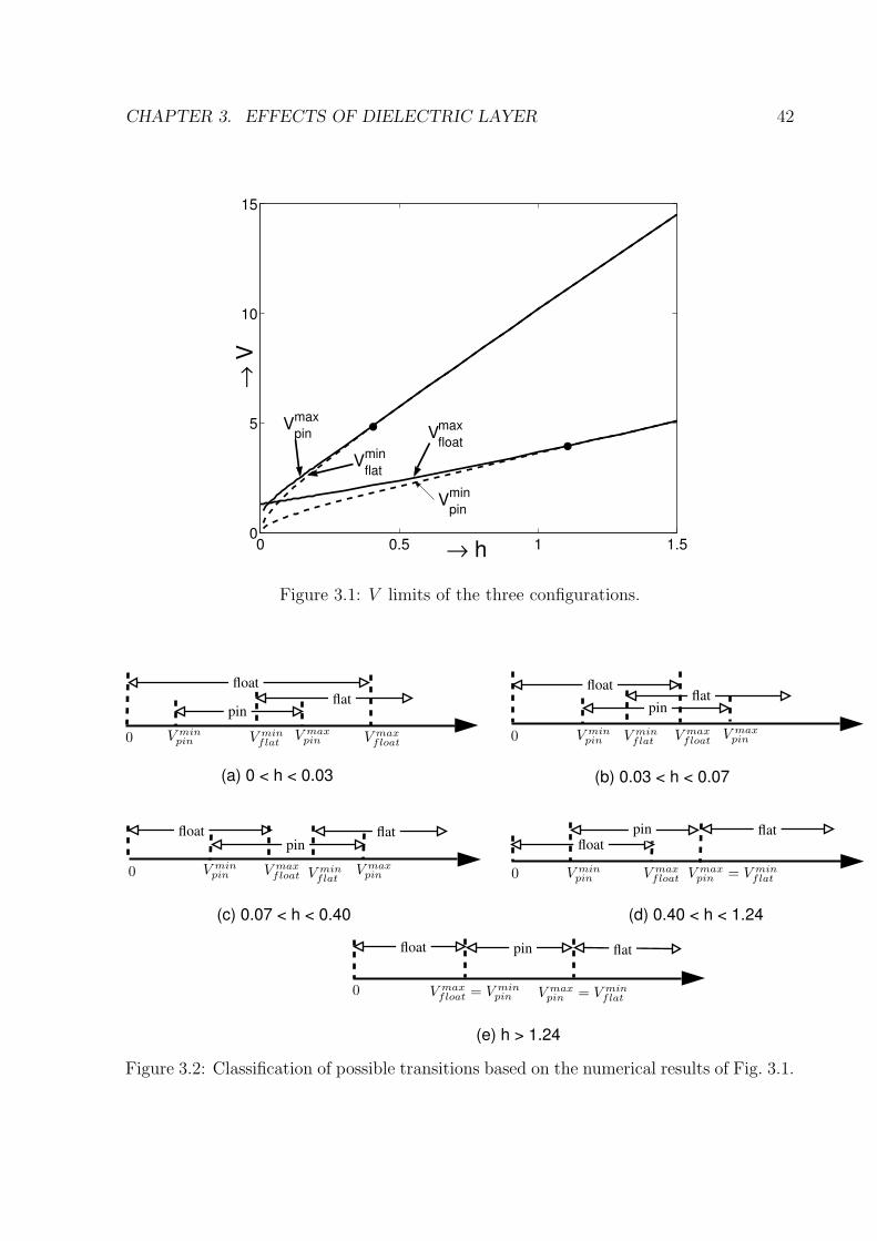
V limits for the three configurations, computed for varying h values, are shown in Fig. 3.1.
Possible transitions between configurations are shown in Fig. 3.2, based on Fig. 3.1.
3.3 Transitions
Four transitions are identified, as suggested by Fig. 3.2. The following insights into
transitions from one configuration to another would be impossible with lumped parameter
models, and somewhat obscured with 3-D models. These simple insights form one of the
main benefits of the beam model for the actuator.
CHAPTER 3. EFFECTS OF DIELECTRIC LAYER 42
0 0.5 1 1.50
5
10
15
→ h
→ V
Vpinmin
VfloatmaxV
pinmax
Vflatmin
• •
Figure 3.1: V limits of the three configurations.
1
(c) 0.07 < h < 0.40
(b) 0.03 < h < 0.07
(e) h > 1.24
(d) 0.40 < h < 1.24
(a) 0 < h < 0.03
PSfrag replacements
float
float
float
float
float
pin
pin
pin
pin
pin
flat
flat
flat
flat
flat
0
0
0
0
0
V minpin
V minpin
V minpin
V minpin
V maxpin V max
pin
V maxpin
V minflat
V minflat
V minflat
V maxfloat
V maxfloat
V maxfloat
V maxfloat V max
pin = V minflat
V maxpin = V min
flatV max
float = V minpin
Figure 3.2: Classification of possible transitions based on the numerical results of Fig. 3.1.

CHAPTER 3. EFFECTS OF DIELECTRIC LAYER 43
0 0.5 1 1.50
0.2
0.4
0.6
h
Jum
p at
free
end
Figure 3.3: Variation of the magnitude of the pull-in discontinuity with h.
3.3.1 Pull-In
Pull-in occurs when the floating configuration solution disappears, as discussed earlier.
Figure 3.3 shows the magnitude of the pull-in discontinuity for varying h values. The jump
in the height at the free end of the beam at the point of transition results from a turning
point bifurcation, as discussed later. Here, we note (Fig. 3.3) that the magnitude decreases
essentially linearly with increasing h. It is interesting to note that for h < 0.03 (Fig.
3.2(a)), the transition from floating has to be to the flat configuration. For 0.03 < h < 0.07
(Fig. 3.2(b)), the transition could be to either the pinned or the flat configuration, and only
a full nonlinear dynamic analysis (not attempted here) can resolve which configuration is
reached immediately after pull-in. For h > 0.07, the transition has to be to the pinned
configuration. Upon increasing the voltage, regardless of h, any pinned configuration will
transition to a flat configuration.

CHAPTER 3. EFFECTS OF DIELECTRIC LAYER 44
0.2 0.4 0.6 0.8 1 1.20
0.5
1
1.5
→ V
→ −
(Slo
pe)
h = 0.01
Figure 3.4: Pull-down: jump in slope at the touching end of the beam.
3.3.2 Pull-Down
The transition from the pinned to the flat configuration is referred to here as pull-down.
The pinned configuration has a nonzero slope at the beam’s end point, while the flat
configuration has zero slope. As is the case for pull-in, a discontinuous transition from
pinned to flat occurs due to a turning point bifurcation, as discussed later. Figure 3.4
shows the pull-down discontinuity decreases faster and faster, until the curve turns around
(not shown here; see discussion later) and the pinned solution disappears. Figure 3.5
shows the magnitude of the pull-down slope discontinuity for different h. For h > 0.4, the
discontinuity in the transition disappears.
3.3.3 Pull-Up
Starting in the flat configuration, a transition is possible to a pinned configuration. Here,
we refer to such a transition as pull-up. Again, for h > 0.4, pull-up is continuous (Fig. 3.2).
CHAPTER 3. EFFECTS OF DIELECTRIC LAYER 45
0 0.5 1 1.50
0.1
0.2
0.3
0.4
0.5
0.6
0.7
0.8
0.9
1
→ h
→ M
agni
tutd
e of
jum
p in
the
slop
e
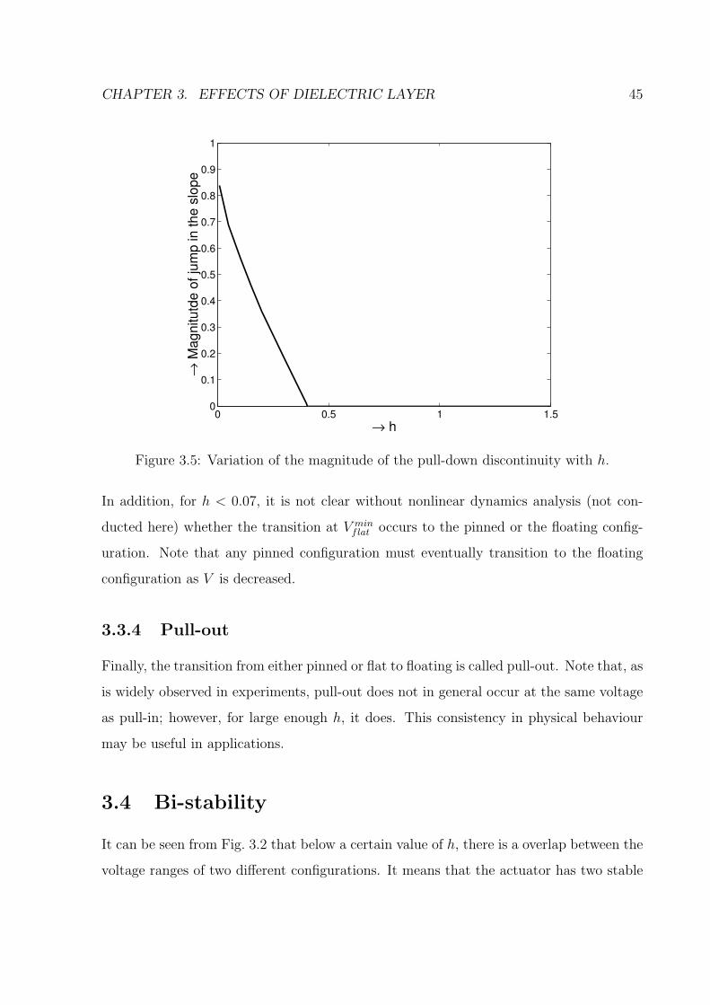
Figure 3.5: Variation of the magnitude of the pull-down discontinuity with h.
In addition, for h < 0.07, it is not clear without nonlinear dynamics analysis (not con-
ducted here) whether the transition at V minflat occurs to the pinned or the floating config-
uration. Note that any pinned configuration must eventually transition to the floating
configuration as V is decreased.
3.3.4 Pull-out
Finally, the transition from either pinned or flat to floating is called pull-out. Note that, as
is widely observed in experiments, pull-out does not in general occur at the same voltage
as pull-in; however, for large enough h, it does. This consistency in physical behaviour
may be useful in applications.
3.4 Bi-stability
It can be seen from Fig. 3.2 that below a certain value of h, there is a overlap between the
voltage ranges of two different configurations. It means that the actuator has two stable

CHAPTER 3. EFFECTS OF DIELECTRIC LAYER 46
0.2 0.4 0.6 0.8 1 1.2 1.40
0.1
0.2
0.3
0.4
0.5
0.6
0.7
0.8
0.9
1
→ h
→ W
idth
of b
i−st
abili
ty re
gion
Floating − Pinned configurationPinned − Flat configuration
Figure 3.6: Variation of width of bi-stability region with h.
solutions in the overlap region and it can stay in either of the states. This is known as
hysteresis or bi-stability.
The width of bi-stability regions between the floating-pinned and the pinned-flat con-
figurations, as a function of h, is shown in Fig. 3.6. Bi-stability between the pinned
and flat configurations disappears for h > 0.4. Similarly, there is no bi-stability between
floating and pinned configurations for h > 1.24.
Note that for h < 0.07, there are three stable states for certain values of V . Therefore,
there is a tri-stability for h < 0.07. The existence of tri-stable states has not previously
been noted for such actuators in the literature.
3.5 Discussion and Conclusions
Voltage limits are computed for all the three possible configurations. A frame work of
all possible types of transitions is made based on the overlaps in voltage ranges of these
configurations. Tri-stable states are observed for the first time for very small values of h.
With the increase in dielectric layer thickness, magnitude of the discontinuities and width

CHAPTER 3. EFFECTS OF DIELECTRIC LAYER 47
of bi-stability regions decreases. For h > 1.24, all the transitions are continuous and the
bi-stable states disappear. Hence, the actuator has a smooth, predictable and reversible
behaviour for larger value of h.
Chapter 4
Dynamic Stability of Equilibrium
Solutions
4.1 Introduction
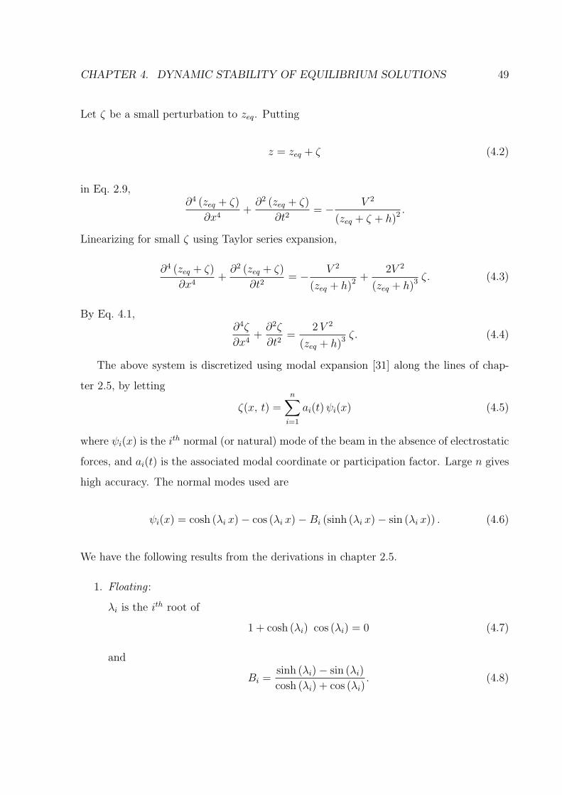
The governing Eq. 2.10 is nonlinear and hence, it can have multiple equilibrium solutions.
The solution obtained depends on the initial guess. Some of these solutions are infeasible
as they penetrate into the dielectric layer. Physically feasible equilibrium solutions may or
not be dynamically stable. In this chapter, we perform the dynamic stability analysis of
all the physically feasible equilibrium solutions in the floating and pinned configurations.
The correlation of these results to chapter 3 is also discussed.
4.2 Method
The dynamic stability of an equilibrium solution can be determined by considering small
variations of that solution, and is governed by an eigenvalue problem.
Let zeq be an equilibrium solution. Then
∂4zeq∂x4
= − V 2
(zeq + h)2 (4.1)
48
CHAPTER 4. DYNAMIC STABILITY OF EQUILIBRIUM SOLUTIONS 49
Let ζ be a small perturbation to zeq. Putting
z = zeq + ζ (4.2)
in Eq. 2.9,∂4 (zeq + ζ)
∂x4+∂2 (zeq + ζ)
∂t2= − V 2
(zeq + ζ + h)2 .
Linearizing for small ζ using Taylor series expansion,
∂4 (zeq + ζ)
∂x4+∂2 (zeq + ζ)
∂t2= − V 2
(zeq + h)2 +2V 2
(zeq + h)3 ζ. (4.3)
By Eq. 4.1,∂4ζ
∂x4+∂2ζ
∂t2=
2V 2
(zeq + h)3 ζ. (4.4)
The above system is discretized using modal expansion [31] along the lines of chap-
ter 2.5, by letting
ζ(x, t) =n∑i=1
ai(t)ψi(x) (4.5)
where ψi(x) is the ith normal (or natural) mode of the beam in the absence of electrostatic
forces, and ai(t) is the associated modal coordinate or participation factor. Large n gives
high accuracy. The normal modes used are
ψi(x) = cosh (λi x)− cos (λi x)−Bi (sinh (λi x)− sin (λi x)) . (4.6)
We have the following results from the derivations in chapter 2.5.
1. Floating :
λi is the ith root of
1 + cosh (λi) cos (λi) = 0 (4.7)
and
Bi =sinh (λi)− sin (λi)
cosh (λi) + cos (λi). (4.8)

CHAPTER 4. DYNAMIC STABILITY OF EQUILIBRIUM SOLUTIONS 50
2. Pinned :
λi is the ith root of
coth (λi)− cot (λi) = 0 (4.9)
and
Bi = coth (λi) . (4.10)
Stability analysis of the flat configuration is more difficult because the contacting length of
the beam changes during motion. Such an analysis is not attempted here. Note, however,
that an extended contact region suggests, intuitively, that the flat configuration is stable.
The normal modes are, as the name suggests, orthonormal:
1∫0
ψi(x)ψj(x) dx =
1 if i = j,
0 otherwise.(4.11)
From Eq. 4.6,∂4ψi(x)
∂x4= λ4
iψi(x) (4.12)
Equation 4.4 becomes
n∑i=1
[∂2ai(t)
∂t2ψi(x) + λ4
i ai(t)ψi(x)
]≈ 2V 2
(zeq + h)3
n∑i=1
ai(t)ψi(x), (4.13)
where we write “≈” instead of “=” to emphasize that a finite-n approximation is being
made.
Multiplying the above with ψj(x), j = 1, 2, · · · , n, and integrating over the length, we
obtain
∂2aj(t)
∂t2+ λ4
j aj(t) =n∑i=1
ai(t)
1∫0
2V 2
(zeq + h)3 ψi(x)ψj(x) dx, (4.14)
where we have reintroduced “=” instead of “≈” for convenience, although the finite-n
approximation remains. Note, also, that the integral on the right hand side requires
knowledge of zeq(x) from a separate calculation.

CHAPTER 4. DYNAMIC STABILITY OF EQUILIBRIUM SOLUTIONS 51
In matrix form,∂2~a
∂t2+ Λ4~a−B~a = 0 (4.15)
where
~a = [ a1(t), a2(t), a3(t), · · · · · · an(t) ]T (4.16)
and Λ is a diagonal matrix with Λjj = λj. Also, B is a square matrix with
Bij =
1∫0
2V 2
(zeq + h)3 ψi(x)ψj(x) dx. (4.17)
Let ~a = ~u eσt. Substituting in Eq. 4.15,
(−Λ4 +B)~u = σ2 ~u. (4.18)
The eigenvalues of the above system determine stability. By the symmetry of Λ and
B, all σ2 are real. If all σ2 are negative, then all solutions are linear combinations of
sinusoidal oscillations; and the original equilibrium solution is dynamically stable. A
positive σ2 implies instability. At a stability boundary, one eigenvalue will be σ2 = 0 (a
degenerate case).
Rigorous analysts will note that such stability only holds within the linear approx-
imation and is neutral at best; deeper analysis is required, in principle and for general
problems, to resolve rigorously whether small perturbations or nonlinearities or errors
from finite n can actually make the system unstable. However, experience with vibra-
tions of other conservative systems in engineering suggests that the stability condition
used here is reliable. The results obtained below are also intuitively acceptable. In any
case, an equilibrium solution found to be unstable by this method certainly is much more
unstable than any weak instabilities that might conceivably exist in the solutions found to
be stable by the truncated (finite-n) linear analysis. Thus, this analysis acts as a reliable
discriminator between strongly unstable solutions and solutions that are probably stable
but failing that are, at most, very weakly unstable.
CHAPTER 4. DYNAMIC STABILITY OF EQUILIBRIUM SOLUTIONS 52
Note that the numerical integration to be performed in Eq. 4.17 requires zeq and ψ
values at the mesh points. Of these, zeq was computed above at a number of mesh points;
and ψ was given above. All integrations were performed using Simpson’s rule. Three
normal modes were used in the stability analysis.
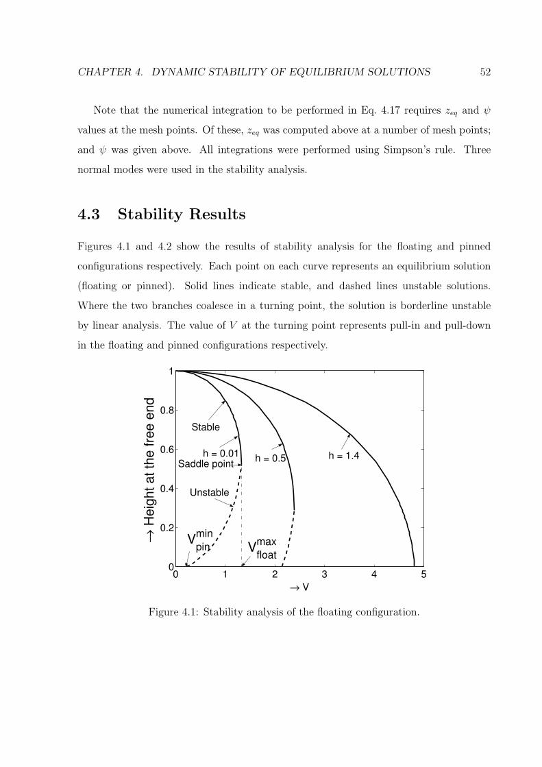
4.3 Stability Results
Figures 4.1 and 4.2 show the results of stability analysis for the floating and pinned
configurations respectively. Each point on each curve represents an equilibrium solution
(floating or pinned). Solid lines indicate stable, and dashed lines unstable solutions.
Where the two branches coalesce in a turning point, the solution is borderline unstable
by linear analysis. The value of V at the turning point represents pull-in and pull-down
in the floating and pinned configurations respectively.
0 1 2 3 4 50
0.2
0.4
0.6
0.8
1
→ V
→ H
eigh
t at t
he fr
ee e
nd
Stable
Unstable
h = 0.5 h = 0.01 h = 1.4 Saddle point
Vfloatmax V
pinmin
Figure 4.1: Stability analysis of the floating configuration.
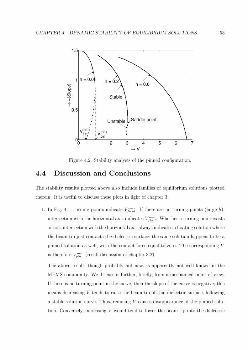
CHAPTER 4. DYNAMIC STABILITY OF EQUILIBRIUM SOLUTIONS 53
0 1 2 3 4 5 6 70
0.5
1
1.5
→ V
→ −
(Slo
pe)
Stable
Unstable
h = 0.2 h = 0.01 h = 0.6
Saddle point
Vpinmax V
flatmin
Figure 4.2: Stability analysis of the pinned configuration.
4.4 Discussion and Conclusions
The stability results plotted above also include families of equilibrium solutions plotted
therein. It is useful to discuss these plots in light of chapter 3.
1. In Fig. 4.1, turning points indicate V maxfloat. If there are no turning points (large h),
intersection with the horizontal axis indicates V maxfloat. Whether a turning point exists
or not, intersection with the horizontal axis always indicates a floating solution where
the beam tip just contacts the dielectric surface; the same solution happens to be a
pinned solution as well, with the contact force equal to zero. The corresponding V
is therefore V minpin (recall discussion of chapter 3.2).
The above result, though probably not new, is apparently not well known in the
MEMS community. We discuss it further, briefly, from a mechanical point of view.
If there is no turning point in the curve, then the slope of the curve is negative; this
means decreasing V tends to raise the beam tip off the dielectric surface, following
a stable solution curve. Thus, reducing V causes disappearance of the pinned solu-
tion. Conversely, increasing V would tend to lower the beam tip into the dielectric
CHAPTER 4. DYNAMIC STABILITY OF EQUILIBRIUM SOLUTIONS 54
surface, bringing a vertical contact force into play and producing a pinned solution.
Hence, the intersection marks V minpin .
On the other hand, if there is a turning point, then slightly raising V produces a
floating solution where the beam tip is slightly above the dielectric surface. How-
ever, that solution is unstable, and so a slight downward perturbation to it will cause
the beam tip to come down further until it touches the dielectric surface, producing
a pinned solution. Conversely, lowering V slightly would make the beam tip tend
to dip below the dielectric surface; this would bring into play an upward acting
contact force, disturbing the solution; and, the solution being unstable, would make
the beam move further up, away from the pinned state.
In this way, simultaneous consideration of equilibrium and stability helps us under-
stand why the intersection point of the floating solution curve with the horizontal
axis indicates V minpin .
2. Similarly, considering the pinned configuration illustrated in Fig. 4.2 (the vertical
axis shows the slope at the end of the beam), we observe that V maxpin is the maximum
V at which a stable solution exists (whether there is a turning point or not), and
the solution curve intersects the horizontal-axis at V minflat .
3. For h > 0.4, all pinned solutions are stable. In other words, V maxpin = V min
flat . Simulta-
neously stable pinned and flat solutions no longer coexist (this mode of bi-stability
disappears).
4. For h > 1.24, all floating solutions are stable, and V maxfloat = V min
pin . Simultaneous
multiple stable solutions of any kind no longer exist.
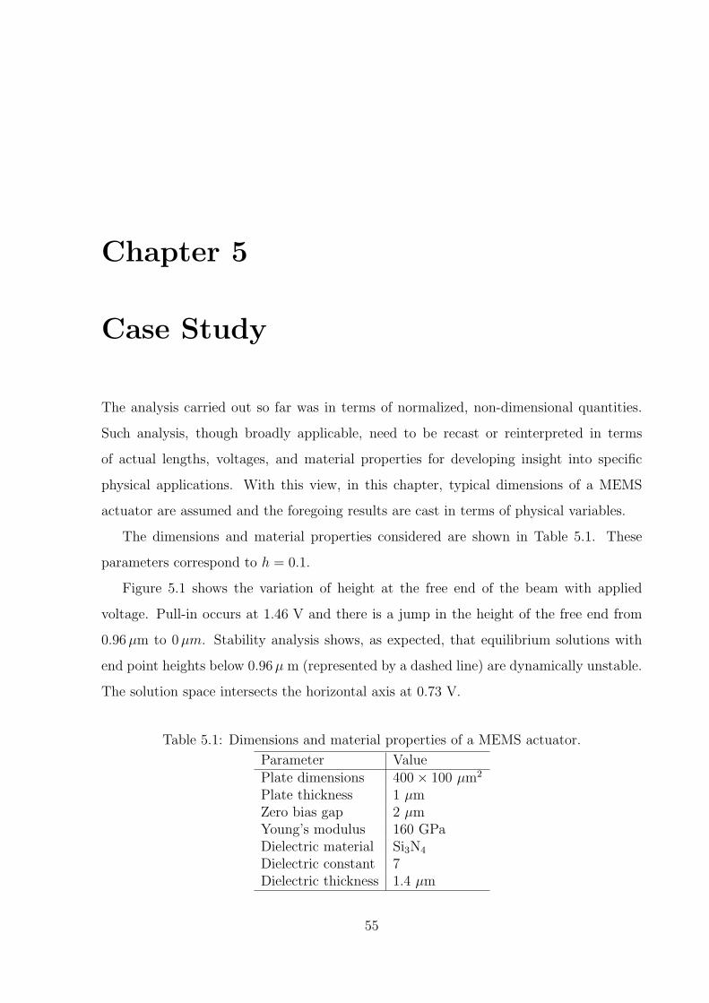
Chapter 5
Case Study
The analysis carried out so far was in terms of normalized, non-dimensional quantities.
Such analysis, though broadly applicable, need to be recast or reinterpreted in terms
of actual lengths, voltages, and material properties for developing insight into specific
physical applications. With this view, in this chapter, typical dimensions of a MEMS
actuator are assumed and the foregoing results are cast in terms of physical variables.
The dimensions and material properties considered are shown in Table 5.1. These
parameters correspond to h = 0.1.
Figure 5.1 shows the variation of height at the free end of the beam with applied
voltage. Pull-in occurs at 1.46 V and there is a jump in the height of the free end from
0.96µm to 0µm. Stability analysis shows, as expected, that equilibrium solutions with
end point heights below 0.96µ m (represented by a dashed line) are dynamically unstable.
The solution space intersects the horizontal axis at 0.73 V.
Table 5.1: Dimensions and material properties of a MEMS actuator.
Parameter ValuePlate dimensions 400× 100 µm2
Plate thickness 1 µmZero bias gap 2 µmYoung’s modulus 160 GPaDielectric material Si3N4
Dielectric constant 7Dielectric thickness 1.4 µm
55

CHAPTER 5. CASE STUDY 56
0 0.5 1 0
0.2
0.4
0.6
0.8
1
1.2
1.4
1.6
1.8
2
→ Applied voltage (V)
Hei
ght a
t the
free
end
(µ m
)
0.73
Vpinmin
Stable
Unstable
1.46
Vfloatmax = V
pullin
Figure 5.1: Floating configuration: Variation of height at the free end of the beam withapplied voltage.
Figure 5.2 shows the force at the contact point of the cantilever beam vs. applied
voltage for the pinned beam boundary conditions. The sign convention is that negative
values indicate an upward mechanical contact force acting from the dielectric on the end
point of the beam. At 0.73 V, the contact force is zero, corresponding to V minpin as discussed
above. This voltage matches, as it must, the voltage at which the floating solution curve
intersects the x-axis. Figure 5.3 shows the variation of slope at the contact point with
the applied voltage. Pull-down occurs at 2.05 V and the slope at the contact point jumps
from −2.99 × 10⁻³ to 0. Note that this (non-dimensional) slope is small compared to
unity, showing post facto that the linear behaviour assumed in the beam mechanics (as
opposed to the electrostatic loading) is valid.
Solutions with contact point slope below −2.99× 10⁻³ (represented by a dashed line)
are unstable. The solution space intersects the x-axis at 1.76 V.
Figure 5.4 shows the variation of the contact length of the cantilever beam vs. applied
voltage in the flat configuration. V minflat from the figure is 1.76 V. As discussed above, this
voltage matches the voltage at which the pinned solution curve intersects the horizontal

CHAPTER 5. CASE STUDY 57
0.5 1 1.5 2−2
−1.8
−1.6
−1.4
−1.2
−1
−0.8
−0.6
−0.4
−0.2
0
Applied voltage (V)
Con
tact
forc
e (µ
N )
Vpinmin V
pinmax
Figure 5.2: Pinned configuration: Contact force at the touching end of the beam vs.applied voltage.
axis. Figure 5.5 summarizes the voltage ranges of all the three configurations.
Figure 5.6 shows the capacitance-voltage (C-V) characteristics of the actuator in the
floating configuration. The capacitance at zero potential is 0.161 pF and at the pull-in
voltage is 0.201 pF. Hence, within the restrictions of the present model, the actuator has
a tunability of 25 % in the floating configuration (this proportion turns out to be only
weakly dependent on dielectric layer thickness for small values thereof, because the beam
tip is still far from the dielectric layer).
Maximum capacitance in the flat configuration is achieved when the upper plate com-
pletely comes in contact with the dielectric layer: this limit corresponds to V = ∞ and
a breakdown of the beam theory assumptions made in the model. We will retreat from
this limit later; but for now, we write
Cmax =ε0 εr w l
td. (5.1)
For the parameter values used here, Cmax = 1.771 pF. Let C∗ denote the capacitance for

CHAPTER 5. CASE STUDY 58
0.8 1 1.2 1.4 1.6 1.8 20
1
2
3
4
5
6
7x 10
−3
→ Applied voltage (V)
→ −
(Slo
pe)
Stable
Unstable
Vflatmin
Vpinmax=V
pulldown
Figure 5.3: Pinned configuration: Slope at the contact point of the cantilever beam vs.applied voltage.
a non-contact length of l in the flat configuration and let the corresponding voltage be
V ∗. For the parameter values used here, C∗ = 0.621 pF and V ∗ = 1.76 V.
For an arbitrary applied voltage V in the flat regime, let the non-contact length and
the capacitance be a and C respectively.Then
C =a
lC∗ +
ε0 εr w (l − a)
td. (5.2)
Fig. 5.7 shows the C-V characteristics when the minimum non-contact length is limited
to 20 % of the total length of the beam. The voltage range considered is 2.05 – 44 V
to ensure that we stay within the same (flat) configuration. The capacitance range is
0.705 – 1.541 pF, with a tunability of 120 %. Thus, the actuator offers larger tunability
in the flat configuration than in the conventional floating configuration. Unlike in the
floating configuration, the maximum variation in capacitance occurs in the initial part of
the applied voltage range.
We end this chapter with a few qualitative observations. Low dielectric thickness gives

CHAPTER 5. CASE STUDY 59
0 5 10 15 20 25 30 35 40 450
50
100
150
200
250
300
350
→ Applied voltage (V)
→ C
onta
ct le
ngth
(µ m
)
Vflatmin
Figure 5.4: Flat configuration: Contact length of the cantilever beam with the dielectriclayer vs. applied voltage.
1
PSfrag replacements
floatpin
flat
→ Applied voltage (V )0.73 1.46 1.76 2.050
Figure 5.5: Voltage ranges of the three configurations.
greater tunability, but at the cost of discontinuous transitions, multiple coexisting stable
states, and hence less predictable behaviour. These problems can be eliminated with a
high dielectric thickness near the beam tip. However, lower dielectric thickness away from
the beam tip will not cause such problems, while increasing the tunability. In this way, we
anticipate that a dielectric layer of suitably varying thickness may give a large operational
voltage range with both predictable behaviour as well as high tunability.

CHAPTER 5. CASE STUDY 60
0 0.2 0.4 0.6 0.8 1 1.2 1.4
0.165
0.17
0.175
0.18
0.185
0.19
0.195
0.2
→ Applied voltage (Volts)
→ C
apac
itanc
e (p
F)
Tunability = 25 %
Figure 5.6: C-V characteristics in the floating configuration.
5 10 15 20 25 30 35 40
0.8
0.9
1
1.1
1.2
1.3
1.4
1.5
→ Applied Voltage (Volts)
→ C
apac
itanc
e (p
F)
Tunability = 120 %
Figure 5.7: C-V characteristics in the flat configuration.

Chapter 6
Conclusions and Further Work
Cantilever beam electrostatic actuators with an intermediate dielectric layer have been
analyzed in detail over the entire operational range using a beam model.
Three qualitatively different configurations, here called floating, pinned and flat, have
been identified and studied. A scaling law is found in the flat configuration. Transitions
from and to the floating configuration (pull-in and pull-out) and transitions from pinned to
flat (pull-down) and flat to pinned (pull-up) have been studied as well. Bi-stable and tri-
stable states have been found. A classification of all possible types of transitions is made
based on the dielectric layer parameters. Dynamic stability analyses have complemented
the study of these configurations and transitions.
Substrate
Dielectric
Figure 6.1: Proposed designs to achieve more regular and reversible behaviour as well ashigher tunability
61

CHAPTER 6. CONCLUSIONS AND FURTHER WORK 62
Higher dielectric thickness gives more regular and predictable behaviour, at the cost
of lower overall tunability in device characteristics. Hence, designs similar to Fig. 6.1,
with higher dielectric thickness near the free end may result in more regular and reversible
behaviour as well as higher tunability. In the first proposed design, the dielectric thickness
is low over most of the beam and is smoothly increasing to a significantly larger value
near the free end. In the second design, the thickness of the substrate is decreased in
steps near the right end and a dielectric layer is deposited over the substrate with its
outer surface being at a constant height. Such designs may also be useful in achieving
the desired C-V characteristics.
In future works, behaviour of MEMS actuators with varying dielectric thickness can
be studied in detail. Similar analysis can be carried out for fixed-fixed and circularly
clamped MEMS electrostatic actuators.

Bibliography
[1] L. A. Rocha, E. Cretu, and R. F. Wolffenbuttel, “Full characterisation of pull-in in
single-sided clamped beams,” Sensors Actuators A, vol. 110, pp. 301–309, Feb. 2004.
[2] V. Shrivastava, N. R. Aluru, and S. Mukherjee, “Numerical analysis of 3D electro-
statics of deformable conductors using a Lagrangian approach,” Engineering Analysis
with Boundary Elements, vol. 28, no. 6, pp. 583–591, June 2004.
[3] M. I. Younis, E. M. Abdel-Rahman, and A. H. Nayfeh, “A reduced-order model
for electrically actuated microbeam-based MEMS,” IEEE J. Microelectromechanical
Systems, vol. 12, no. 5, pp. 672–680, Oct. 2003.
[4] E. M. Abdel-Rahman, M. I. Younis, and A. H. Nayfeh, “Characterization of the
mechanical behavior of an electrostatically actuated microbeam,” J. Micromech. Mi-
croeng., vol. 12, no. 6, pp. 759–766, Nov. 2002.
[5] S. D. Senturia, Microsystem Design. Boston, MA: Kulwer Academic, 2001.
[6] G. M. Rebeiz, RF MEMS: Theory, Design and Technology. New Jersey: John Wiley
and Sons, 2003.
[7] R. K. Gupta, “Electrostatic Pull-In test structure design for in-situ mechanical prop-
erty measurements of microelectromechanical systems (MEMS),” Ph.D. dissertation,
MIT, June 1997.
[8] E. S. Hung and S. D. Senturia, “Generating efficient dynamic models for microelec-
tromechanical systems from a few finite element simulation runs,” IEEE J. Micro-
electromechanical Systems, vol. 8, no. 3, pp. 280–289, Sep. 1999.
63

BIBLIOGRAPHY 64
[9] L. D. Gabby, J. E. Mehner, and S. D. Senturia, “Computer-aided generation of
reduced-order dynamic macromodels-I: Non-stress-stiffened case,” IEEE J. Micro-
electromechanical Systems, vol. 9, no. 2, pp. 262–269, June 2000.
[10] S. D. Senturia, “CAD challenges for microsensors, microactuators and microsystems,”
in Proc. IEEE, vol. 86, Aug. 1998, pp. 1611–1626.
[11] J. A. Pelesko, “Mathematical modeling of electrostatic MEMS with tailored dielectric
properties,” SIAM J. Appl. Math., vol. 62, no. 3, pp. 888 – 908, Jan. 2002.
[12] C. Goldsmith, J. Randall, S. Eshelman, T. H. Lin, D. Denniston, S. Chen, and
B. Norvell, “Characteristics of micromachined switches at microwave frequencies,”
in IEEE MTT-S International Microwave Symposium Digest, vol. 2, San Francisco,
June 1996, pp. 1141–1144.
[13] J. B. Muldavin and G. M. Rebeiz, “High-isolation CPW MEMS shunt switches. 1.
Modeling,” IEEE Trans. Microwave Theory Tech., vol. 48, no. 6, pp. 1045 – 1052,
June 2000.
[14] E. S. Hung and S. D. Senturia, “Tunable capacitors with programmable capacitance-
voltage characteristic,” in Solid-State Sensors and Actuators Workshop, June 1998,
pp. 292–295.
[15] G. V. Ionis, A. Dec, and K. Suyama, “A zipper-action differential micro-mechanical
tunable capacitor,” in Proceedings of MEMS Conference, Aug. 2001, pp. 24–26.
[16] T. Ketterl, T. Weller, and D. Fries, “A micromachined tunable CPW resonator,” in
IEEE MTT-S International Microwave Symposium Digest, vol. 1, Phoenix, AZ, May
2001, pp. 345–348.
[17] H. C. Nathanson, W. E. Newell, R. Wickstrom, and J. R. Davis, “The resonant gate
transistor,” IEEE Transactions on Electron Devices, vol. ED-14, no. 3, pp. 117–133,
Mar. 1967.

BIBLIOGRAPHY 65
[18] H. A. C. Tilmans, “Equivalent circuit representation of electromechanical transduc-
ers: I. lumped-parameter systems,” J. Micromech. Microeng., vol. 6, no. 1, pp. 157–
176, Mar. 1996.
[19] A. Dec and K. Suyama, “Micromachined electro-mechanically tunable capacitors and
their applications to RF IC’s,” IEEE Trans. Microwave Theory Tech., vol. 46, no. 12,
pp. 2587–2596, Dec. 1998.
[20] S. Pamidighantam, R. Puers, K. Baert, and H. A. C. Tilmans, “Pull-in voltage
analysis of electrostatically actuated beam structures with fixed-fixed and fixed-free
end conditions,” J. Micromech. Microeng., vol. 12, no. 4, pp. 458–464, July 2002.
[21] J. R. Gilbert, R. Legtenberg, and S. D. Senturia, “3D coupled electromechanics
for MEMS: Applications of CoSolve-EM,” in Proc. of the Int. Conf. on MEMS,
Amsterdam, The Netherlands, 1995, pp. 122–127.
[22] J. R. Gilbert, G. K. Ananthasuresh, and S. D. Senturia, “3D modeling of contact
problems and hysteresis in coupled electro-mechanics,” in Proc. of Ninth Int. Work-
shop on Microelectromechanical Systems, Feb. 1996, pp. 127–132.
[23] E. K. Chan, K. Garikipati, and R. W. Dutton, “Characterization of contact elec-
tromechanics through capacitance-voltage measurements and simulations,” IEEE J.
Microelectromechanical Systems, vol. 8, no. 2, pp. 208–217, June 1999.
[24] E. K. L. Chan, “Characterization and modeling of electrostatically actuated polysil-
icon micromechanical devices,” Ph.D. dissertation, Stanford University, Nov. 1999.
[25] M. Abramowitz and I. A. Stegun, Handbook of Mathematical Functions with Formu-
las, Graphs, and Mathematical Tables. Dover, 1972.
[26] [Online]. Available: http://mathworld.wolfram.com/CubicFormula.html
[27] G. M. Rebeiz and J. B. Muldavin, “RF MEMS switches and switch circuits,” IEEE
microwave magazine, vol. 2, no. 4, pp. 59–71, Dec. 2001.

BIBLIOGRAPHY 66
[28] C. H. Mastrangelo and C. H. Hsu, “A simple experimental technique for the mea-
surement of the work of adhesion of microstructures,” in Technical Digest- IEEE
Solid-State Sensor and Actuator Workshop, 1992, pp. 208–212.
[29] M. P. de Boer and T. A. Michalske, “Accurate method for determining adhesion of
cantilever beams,” Journal of Applied Physics, vol. 86, pp. 817–827, July 1999.
[30] W. H. Press, S. A. Teukolsky, W. T. Vetterling, and B. P. Flannery, Numerical recipes
in C: The art of scientific computing. Cambridge University Press, 1992.
[31] A. H. Nayfeh and P. F. Pai, Linear and Nonlinear Structural Mechanics. New Jersey:
Wiley-Interscience, 2004.