and

r-

Unclas15330

UNIVERSITY, ALABAMA

Rep~~duced- by

NATIONAL TECHNICALINFORMATION SERVICE

U 5 Deportment of CommerceSpringfield VA 22151

October, 1971

by

RONALD C. HOUTSProject Director

JERRY D. MOOREResearch Associate

TECHNICAL REPORT NUMBER 135-102

CHARACTERIZATION OF It1PUlSE NOISE AND

ANALYSIS OF ITS EFFECTS UPON

CORRELATION RECEIVERSe~-/"J3~1/

BUREAU OF ENGINEERING RESEARCH

UNIVERSITY OF ALABAMA

..:~ .'-J,,-,~,

-~. COMMUNICATION SYSTEMS GROUP

https://ntrs.nasa.gov/search.jsp?R=19720014479 2018-05-26T15:28:19+00:00Z

CHARACTERIZATION OF IMPULSE NOISE

AND ANALYSIS OF ITS EFFECTS UPON

CORRELATION RECEIVERS

by

RONALD C. HOUTSProject Director

and

JERRY D. MOOREResearch Associate

October, 1971

TECHNICAL REPORT NUMBER 135-102

Prepared for

National Aeronautics and Space AdministrationGeorge C. Marshall Space Flight Center

Huntsville, Alabama

Under Contract Number

NAS8-20172

Communication Systems GroupBureau of Engineering Research

University of Alabama

ABSTRACT

A noise model is formulated to describe the impulse noise in many

digital systems. A simplified model, which assumes that each noise

burst contains a randomly weighted version of the same basic waveform,

is used to derive the performance equations for a correlation receiver.

The expected number of bit errors per noise burst is expressed as a

function of the average signal energy, signal-set correlation coef­

ficient, bit time, noise-weighting-factor variance and probability

density function, and a time range function which depends on the cross­

correlation of the signal-set basis functions and the noise waveform.

A procedure is established for extending the results for the simplified

noise model to the general model. Unlike the performance results for

Gaussian noise, it is shown that for impulse noise the error perfor~

mance is affected by the choice of signal-set basis functions and that

Orthogonal signaling is not equivalent to On-Off signaling with the

same average energy. The error performance equations are upper bounded

by a procedure which removes the dependence on the noise waveform and

the signal-set basis functions. A looser upper bound which is also in­

dependent of the noise-weighting-factor probability density function is

obtained by applying Chebyshev's inequality to the previous bound result.

It is shown that the correlation receiver is not optimum for impulse

noise because the signal and noise are correlated and the error perfor­

mance can be improved by" inserting a properly specified nonlinear device

prior to the receiver input.

ii

ACKNOWLEDGEMENT

The authors would like to express their appreciation to the

personnel of the Telemetry and Data Technology Branch, Marshall

Space Flight Center, for their useful technical consulations. In

particular, Messrs. Frost, Emens, and Coffey have rendered valuable

assistance and direction. Also, the technical discussions with

Messrs. Perry and Stansberry of SCI Electronics Inc. were very help­

ful. A significant portion of the computer programming for this

investigation was performed by Mr. R. H. Curl.

iii

TABLE OF CONTENTS

ABSTRACT...•.

ACKNOWLEDGEMENT •

LIST OF FIGURES •

LIST OF TABLES.

CHAPTER 1 INTRODUCTION.

1.1 STATEMENT OF PROBLEM.

1.2 IMPULSE NOISE LITERATURE REVIEW.

1.3 APPROACH OUTLINE.

CHAPTER 2 IMPULSE NOISE MODEL. .

2.1 HEURISTIC CONSIDERATIONS.

2.2 MATHEMATICAL MODEL...

2.3 NOISE CHARACTERISTICS.

CHAPTER 3 CORRELATION RECEIVER PERFORMANCE ANALYSIS.

Page

ii

iii

vi

viii

1

. . . . 1

2

4

5

5

7

10

15

3.1 GENERAL OBSERVATIONS.•.. 15

3.2 DERIVATION OF GENERALIZED ERROR PERFORMANCEEQUATION.. ..............•.• 21

CHAPTER 4

3.3 PERFORMANCE EQUATIONS FOR SPECIFIC SIGNALSETS. . . . . • . .• ....

3.4 DERIVATION OF PERFORMANCE BOUNDS.

SPECIFIC PERFORMANCE RESULTS .

32

35

40

4.1 GENERALIZED IMPULSE NOISE WAVEFORMS. 40

4.2 PERFORMANCE RESULTS FOR DECAYING EXPONENTIAL. 43

iv

4.3 PERFORMANCE RESULTS FOR EXPONENTIALLY­DECAYING SINUSOID . . . . . . . . . • • 53

4.4 EFFECT OF SIGNAL AND NOISE CORRELATION. . 56

4.5 COMPARISON TO RESULTS FROM THE LITERATURE. 56

CHAPTER 5 METHODS FOR IMPROVING RECEIVER PERFORMANCE . .

5.1 SURVEY OF RECOMMENDATIONS FOR IMPROVEDRECEIVER DESIGNS. . . .. ....•

5.2 PERFORMANCE ANALYSIS FOR A NONLINEARCORRELATION RECEIVER. . . . . . . .

5.3 COMPARISON OF LINEAR AND NONLINEARCORRELATION RECEIVERS . . .

59

59

61

66

CHAPTER 6 CONCLUSIONS AND RECOMMENDATIONS.

6.1 CONCLUSIONS . . ..73

73

6.2 RECOMMENDATIONS FOR FURTHER STUDY

APPENDIX A DERIVATION OF POWER-DENSITY SPECTRUM ANDPROBABILITY DENSITY FUNCTIONS FOR THE GIN(UNIQUE WAVEFORM) MODEL . .

A.1 POWER-DENSITY SPECTRUM .

A.2 PROBABILITY DENSITY FUNCTIONS.

APPENDIX B ALTERNATIVE METHOD FOR FINDING THE CONDITIONALBIT ERROR PROBABILITY . .

APPENDIX C COMPUTER PROGRAM: GINIMP

C.1 GENERAL INFORMATION.

C.2 FLOW CHART, PROGRAM LISTING ANDEXPLANATION .

APPENDIX D COMPUTER PROGRAM: LIMITER.

D.1 GENERAL INFORMATION..

74

76

76

78

86

89

89

90

102

102

D.2 FLOW CHART, PROGRAM LISTING AND EXPLANATION.. 103

LIST OF REFERENCES.

UNCITED REFERENCES.

v

114

118

LIST OF FIGURES

Figure Page

2-1

3-1

3-2

3-3

3-4

4-1

4-2

4-3

4-4

4-5

4-6

Impulse Noise Model Waveshapes

Digital Communication System

Correlation Receiver .

Interpretation of Time Range TR1

(n).

Performance Bounds •

Decaying-Exponential Waveforms

Five Typical Signal Sets .

Effect of Weighting Factor P.D.F. on UnipolarSignaling in the Presence of Decaying-ExponentialNoise with 0.2 ms Time Constant•.•..••

Effect of Decaying-Exponential Waveform TimeConstant on Performance of Unipolar Signaling.

Performance of ASK Signaling for VariousDecaying-Exponential Time Constants ••..

Comparison of Unipolar and ASK Signal Setsfor Decaying-Exponential Waveform. . . . . •

8

20

22

31

39

42

44

46

47

49

50

4-7

4-8

Comparison of Five Signal Sets for Decaying­Exponential Waveform with 0.2 ms Time Constant

Comparison of Unipolar and ASK Signal Sets forExponentially-Decaying Sinusoid. . • . • .

. . . ~ 52

54

4-9

4-10

Comparison of Five Signal-Sets for Exponentially­Decaying-Sinusoid with 1 ms Time Constant.

Comparison of Unipolar and ASK Signal Sets forWaveforms with 1 ms Time Constants . • . •

55

57

5-1 Digital System with Nonlinear CorrelationReceiver . . . . . . . . . . . . . . . . .

vi

62

5-2

5-3

5-4

5-5

5-6

C-1

C-2

D-1

D-2

Limiter Model. . . . . . . .

Effect of Nonlinear Receiver on Unipolar SignalPerformance in the Presence of Decaying-ExponentialNoise with a 0.2 ms Time Constant...•....•.•

Effect of Nonlinear Receiver on ASK SignalPerformance in the Presence of Decaying-ExponentialNoise with a 0.2 ms Time Constant•..•••.•..

Effect of Nonlinear Receiver on ASK SignalPerformance in the Presence of Exponentia11y­Decaying-Sinusoidal Noise with a 2 ms TimeConstant ••........•......

Effect of Nonlinear Receiver on PSK Signal Perfor­mance in the Presence of' Exponentia11y-Decaying­Sinusoidal Noise with a 2 ms Time Constant • •

GINIMP Flow Chart...

GINIMP Program Listing

LIMITER Flow Chart . .

LIMITER Program Listing.

vii

65

67

69

70

71

91

96

104

108

LIST OF TABLES

Table Page

3.1 Normalized Probability Density Functions · 38

C.l Data Card 1 Format and Identification 92

C.2 Data Card 2 Format and Identification · · . . . 92

D.l Data Card 1 Format and Identification · 103

D.2 Data Card 2 Format and Identification · . . . 105

D.3 Data Card 3 Format and Identification · 106

D.4 Data Card 4 Format and Identification · 107

D.5 Data Card 5 Format and Identification 107

viii

CHAPTER 1

INTRODUCTION

1.1 STATEMENT OF PROBLEM

Traditionally, the performance analyses of digital systems have

incorporated ad4itive white Gaussian (~~G) noise to model the inter­

ference introduced by the communication channel. '~ith this assump­

tion it has been shown that the optimum receiver consists of a bank

of correlators, each of which compares the incoming noisy waveform

with one of the possible received noise-free signals. Although the

AWG noise assumption gives satisfactory error rate predictions for

many situations, it has .failed to predict the much higher error

rates observed on some classes of digital systems. Another type of

additive noise, commonly referred to as impulse noise, is currently

being modeled and used to explain this discrepancy on atmospheric

radio channels and both switched and dedicated baseband channels.

The impulse noise models proPQsed in the literature differ in sev­

eral respects, but all impulse noise is characterized by brief

periods of large amplitude excursions, separated by intervals of

quiescent conditions.

The relatively new area of impulse noise analysis suffers from

the problems of nonstandardization and incompleteness. It is diffi­

cult to compare the results of two authors and impossible to obtain

comparison of the major binary signaling techniques, because of the

multitude of noise models, signal sets, analytical methods and

1

2

simplifying assumptions. In this work the primary objective is to

establish a mathematical model that can be used to approximate addi-

tive impulse noise and then apply this model in the error perfor-

mance analysis for a correlation receiver. The secondary goal is to

present a collection of specific performance results from which it

will be possible to draw some general conclusions regarding impulse

noise and its effect on digital systems.

1.2 IMPULSE NOISE LITERATURE REVIEW

Almost all papers concerning impulse noise have been published

since 1960. A wide variety of mathematical models have been proposed

to describe different aspects of impulse noise. Only a few authors

[1,2]* have discussed the noise waveforms obtained from actual systems,

while much emphasis has been placed on empirically obtained amplitude

and/or time distributions for the noise [1,3-8]. Proposed impulse noise

models have assumed such waveforms as the ideal impulse function, with

either constant weight [9] or probabilistic weighting [10,11], and the

unit-impulse response of the channel being studied [12,13]. Another

approach has been to assume various probabilistic descriptions for the

noise at the receiver output [14]. The majority of performance studies

have been limited to the analysis of a specific binary signaling tech-

nique [2,6,12,13,15-20] although several authors [9,11,21-24] have ob-

tained performance curves and compared more than one signal set based

*Enclosed numbers refer to corresponding entries found in List ofReferences.

3

on their assumed noise models. Zeimer [10] and Millard & Kurz [25]

have extended their analyses to the consideration of M--ary signaling.

The basic approach to error analysis for the practical case of a

general noise waveform which can change from one noise burst to another

has been developed by Houts & Moore [11] and forms the foundation of

the work documented here. Although specific performance res~lts were

not obtained for the general model, upper and lower bounds on signal

set error performances were derived.

Signals corrupted by impulse noise are often detected by receiv­

ers that were designed for use in A~lG noise. It is reasonable to ex­

pect that the error performance of these receivers can be improved.

Several receiver-improvement modifications have been proposed [26-30]

based upon intuition or experimental results. The subject of optimum

receiver design for binary signals in the presence of impulse noise

has received limited treatment in the literature. Snyder [31] has

investigated the design of an optimum receiver for VLF atmospheric

noise. The noise model has a combination of MvG noise and impulse

noise generated by exciting a filter with idealized delta functions.

Specific results are not obtained and remain a topic for further

investigation. A different approach has been used by Rappaport &

Kurz [32] who assume that the noise waveform duration is short com­

pared to the bit time and that independent samples can be obtained

by uniformly sampling the received signal.

4

1.3 APPROACH OUTLINE

The first step in any error performance analysis should be the

development of a realistic noise model. Simplifying assumptions are

sometimes included in the model for the purpose of m~king the analysis

mathematically tractable, which in turn aids in understanding the role

played by the various noise parameters. 11owever, the results from such a

model often fail to predict actual system performance. In Chapter 2 a

generalized impulse noise (GIN) model is presented which can be used to

approximate the impu~se nois~ structure in a broad class of digital sys­

tems. In particular, the model is applicable to a baseband ch~nne1 with

near dc response of the type found in telephone circuits and sophisti~

cated avionics systems such as the proposed data bus for NASA's Space

Shuttle vehicle. The performance analysis for a band-limited channel

using a correlation receiver in the presence of impulse noise described

by the GIN model is presented in Chapter 3. In addition, new and more

definitive performance bounds are obtained for typical binary signal

sets. The effects of selecting various noise weighting factor descrip­

tions, signal sets, and noise waveforms are documented in Chapter 4.

Several performance improvement methods are surveyed in Chapter 5 and

specific results are presented for the case where a nonlinear device

is inserted prior to the correlation receiver. The results show that

the performance can be improved; conseauently, the correlation re-

ceiver is not optimum for impulse noise corrupted signals.

CHAPTER 2

IMPULSE NOISE MODEL

A mathematical model is developed which is sufficiently flexible

to approximate the additive impulse noise ~n a broad class of digital

systems. Also, the power-density spectrum and probability density

function (p.d.f.) are established for certain special cases of the

noise model.

2.1 HEURISTIC CONSIDERATIONS

The waveform description of impulse noise depends on the noise

source, the coupling media, and the characteristics of the channel

under observation. Capacitive and inductive coupling along with

switching transients comprise the major methods by which impulse

noise is introduced into a system. For instance, impulse noise in

a channel might be caused by a lightning discharge or engine igni­

tion noise. Telephone and telemetry systems experience noise from

electromechanical relay switching. Other sources include environ­

mental conditions such as shock, vibration, and maintenance disrup­

tions, i.e., a temporary short circuit. These sources have the com­

mon characteristic that the noise produced occurs in bursts of large

amplitude variations separated by relatively long intervals of neg­

ligible amplitude variations. This observation is the foundation

for the mathematical model presented in Section 2.2.

5

The determination of the noise waveforms can be a time consuming

and expensive process. The number of different waveforms encountered

can be very large, and normally the measuring equipment must have

large bandwidth and a capability for handling aperiodic waveforms.

Kurland & Molony [2] experimentally determined and ranked the error

performance for 15 different noise waveforms at various signal-to­

noise ratios (SNR). No pattern appeared to exist in the relative

standing of the various waveforms as the SNR was changed. Fennick

[1] has reported on specific switched telephone lines where 2000 dis­

tinct waveforms have been analyzed. The result was widely varying

amp~itude and phase spectra characteristics. However, when a subset

of approximately 200 of the waveforms were added together, the com­

posite noise spectrum appeared to approximate the channel transfer

characteristic. This would suggest that a weighted unit-impulse

response of the channel could be used as a typical noise waveform,

For dedicated lines such as private telephone lines or a Space Shut­

tle data bus, the channel characteristics will remain constant in

contrast with the switched telephone system. Furthermore, the number

of possible noise sources are greatly reduced. Measurements of noise

which is induced by relay switching have been made on a Space Shuttle

data bus [33,34] and reveal noise bursts composed of a random number

of aperiodic waveforms. It is difficult to describe the shape of the

waveforms from data presented. A reasonable conjecture is that the

waveforms can be modeled as exponentially-decaying sinusoids.

6

7

2.2 MATHEMATICAL MODEL

A typical noise process based on the discussion of Section 2.1

is modeled as the sum of NB bursts and is shown in Fig. 2-la. The

thk burst, bk(t-Tk), occurs at time Tk and is composed of a random

number, NG, of aperiodic waveforms as shown in Fig. 2-lb. In a

restricted special case, a burst consists of only one waveform as

shown in Fig. 2-lc.

The generalized impulse noise (GIN) model is formulated as

n(t)

NB

L bk (t-Tk ),

k=l

o < t < T, NB- n

1,2, ...• (? .1)

It is assumed that each burst, bk(t-Tk), k

duration TFk , viz.,

1, ... , NB, has a finite

(2.2)

Furthermore, each burst is represented as

NG\'1),--'

j=l

(2.3)

where NG is the number of sample functions that occur, gkj(t) is a wave-

form that is chosen at random from the kth

ensemble of sample functions

k{Gl(t), G2 (t), ... , GN(t)} , I kj is a random variable weighting function

d T " h "f h oth 1 f " Aan k" 1S t e occurrence t1me 0 t e J samp e unct1on. s an exam-J

pIe, let the kth

noise burst contain three sample functions, i.e. ,

8

net)

~TF~a) Noise Bursts

b) Example of ~u1tip1e-WaveformBurst

t--(,(.--JL.--~-I-~r---i'"4-or-----'--(ff------------- t

c) Example of Single-Waveform Burst

Fig. 2-1, Impulse Noise Model I'!aveshapes

9

NG = 3, with each chosen from the kth

ensemble {Gl(t), G2(t), G3 (t),

G4(t), GS(t)} which consists of five sample functions. One possible

description for the burst is

(2.4)

Note that the sample functions G1(t), G2(t), G

4(t) did not appear while

GS(t) was present twice.

Three specialized versions of the GIN model are now presented.

Each of these models is formed by restricting the previous model. The

first specialized version restricts each burst to be composed of sample

functions selected from the same ensemble {G1 (t), G2(t), ... , GN(t)},

and will be identified as the GIN (Single Ensemble) model. This allows

a noise burst to be represented by

NG

L';=1

(2. S)

where the k subscript for g.(t) used in (2.3) can be omitted since eachJ

burst is formed from the same ensemble. The second specialized model

is obtained by adding the additional restriction that each burst con-

tains exactly one sample function. Thus,

n(t)

NB

L I k g1

(t-Tk ) .

k=l

(2.6)

Note that gl(t-Tk ) is randomly selected from the same ensemble of sample

functions for each value that k assumes. This model will be called the

10

GIN (Single Function) model. The third specialized version restricts

the sample function of (2.6) to be the same waveform f(t) for each occur-

ence, i.e.,

n(t)

NB

~ Ikf(t-Tk ) .

k=l

(2.7)

This is identified as the GIN (Unique Waveform) model. If f(t) is

chosen to represent the channel unit-impulse response then (2.7) is

similar to the model used by Bellow & Esposito [12] and to the mo~el

suggested by Fennick [1,20]. The idealiz~d impulse used by Ziemer [10]

and Houts & Moore [11] can be obtained by setting f(t)=o(t).

Some of the impo~tant properties of these noise models are pr~-

sented in Section 2.3. It is shown in Chapter 3 that the performance

analysis for the GIN (Unique Waveform) model can be extended to include

the other models as well.

2.3 NOISE CHARACTERISTICS

Several plausible assumptions will be made concerning the ranqom

variables involved in the GIN model. Also, the power-density spectrum

and the p.d.f. for the GIN (Unique Waveform) model will be determined

as functions of the various noise parameters.

The reasonable hypothesis that each sample functions, gkj(t-Tkj

),

is equally likely to occur at any time in the burst time range, 0 to

TFk , leads to a uniform distribution for Tkj , i.e.,

1TF ' 0 < a < TFk .

k

11

(2.8)

Consequently, for statistically independent occurrence times a Poisson

distribution with the average occurrence rate v can be assumed for the

number of waveforms, NG, in a burst time TFk , i.e.,

(2.9)

A similar result applies to the number of noise bursts in tim~ T if then

bursts are equally like~y to occur at any time.

The p.d.f. descriptions for the random variables associated with

burst type, sample function selection, and the weighting factor are

established by the particular system being analyzed. However, it wil~

be assumed that the weighting factor p.d.f., PIk.(i), is symmetricalJ

about a zero mean. This allows both positive and negative versions of

the noise waveforms gkj(t). It is assumed that the statistical descrip­

tions of the noise parameters are not time dependent. For some systems

this will be a valid assumption, while for others it is an approximation

that must be limited to short time periods.

It is shown in Appendix A that the GIN (Unique Waveform) model

yields a one-sided power-density spectrum given by

S (f)n (2.10)

2where vB is the average occurrence rate of the bursts, 0 is the vari-

ance of ~ach weighting factor I kj , and F(f) is the Fourier transform

12

of the noise waveform f(t). The result of (2.10) can be extended to

the GIN (Single Function) model by taking the expected value with

respect to the waveform type, cf., (A.11). Note that the power-

density spectrum of (2.10) depends on the sample function and is a

function of frequency, i.e., the spectrum is not necessarily white.

For the special case where f(t)=o(t), then F(f)=l and white ~oise

results since Sn(f)=2Vb

02 . Similar results have been given for the

idealized impulse noise model by Ziemer [10] and Houts & Moore [11].

The performance results obtained for impulse noise can be co~-

pared with those for AWG noise, by relating the dependent variables.

The convention established for M~G noise is to plot the error proba-

bi1i~y as a function of signa1-to-noise ratio, defined as the r?ti9

of the average signal energy, EAVG

' to the one-sided noise power~

density spectrum, N , i.e.,- 0

SNRE~G

N°

(2,11)

Previous results [11] have shown that the error performance for addi-

tive idealized impulse noise depends on an energy~to-noise parameter

(ENP), viz.,

ENP (2.12)

where Tb

is the bit time. Thus for the idealized impulse noise,

(2.13)

13

For colored Gaussian noise the performance is expressed as a ratio of

signal power to noise power contained in some specified bandwidth. The

compari$on of SNR and ENP for generalized impulse noise would be more

complicated than the simple relation shown by (2.13) and will not be

determined in this work.

An inter~sting characteristic which can be obtained for the GIN

(Unique Waveform) model is the first-order p.d.f. for the noise net),

i.e., p (u). Following the lead of Rice [35], Middleton [36], andn

Ziemer [10], it is shown in Appendix A that when the number of floise

bursts in time T is modeled by a Poisson process with average raten .

p (u)n

[

A A-5/ 24 2 1jJ(4)(x) + + ... , (2.14)

where Am

(2.15)

and x = u/~.(2.16)

The first term in p (u)n

-1vB ' and the third term

-1/2is of order vB ,the second term of order

-r-3/2enclosed by the brackets is of order vB .

Also, the first term assumes the form of a Gaussian distribution, thus

the remaining terms show how Pn(a) approaches Gaussian as vB increases.

14

If th~ Poisson process assumption used to ~stablish (2.14) is

replaced with the assumption that at most one noise burst can occur

in time T , the p.d.f. becomesn

p (a.)n

P[NB=O] 8(0.) + P[NB=l]T

n

00 T

JIn_00 0

PI(i) 8(a.-if(t-t)) dTdi . (2.17)

In receivers where the bit decision is based on sampling the received

signal and comparing to a voltage threshold, the p.d.f. 's of (2.14) and

(2.17) could be used to determine the probability of error. Using

(2.17), the probability that the noise exceeds a positive threshold Vth

is

00

r p (a.) do.n

P[NB=l]T

nPr(i) dTdi, (2.18)

where the region Rth

is defined such that i.f(t-Tl

) > Vth

. The per-

formance of a correlation receiver is determined in Chapter 3.

CHAPTER 3

CORRELATION RECEIVER PERFORMANCE ANALYSIS

The ~xpression for the error performance is derived for a digital

system that uses a correlation receiver. Although the derivation is

limited to the GIN (Unique Waveform) model, a procedure is presented

for extending the results to the unrestricted GIN model. The error

performance is bounded by a function of the aver~ge signal energy, the

signal set correlation cpefficient, and the variance and p.d.f. descr~p­

tion of the noise weighting factor. The bound dependence on the p.d.f.

is removed by applying Chebyshev's ineq4ality.

3.1 GENERAL OBSERVATIONS

A method for judging the error performance of a digital system

is presented in the section. Subsequently, the analysis for the GIN

model is obtained in terms of the GIN (Unique Waveform) model. The

effect of the communication channel on the ana~ysis of the correlation

receiver is discussed. Several assumptions regarding the GIN (Unique

Waveform) model parameters are summari~ed for use in the derivation Of

Section 3.2.

15

3.1.1 Performance Criterion

Two performance criteri? were considered for use in this work:

namely, the probability of bit error and the expected number of bits

in error given a burst has Qccu~red. The probability of bit error

is used extensively for AWG noise analysis. There is some precedent

[6,9-12] for using this criterion in imp~lse noise analysis; how­

ever, the more definitive criterion of the expected number of bits

in error per noise burst has beep employed [20,24] and ~ill be used

in this work. Each method allows an easy comparison of theoretical

and experimental results, since the difference between the experi­

mental numerical average and the theoretical statistical probability

can be made arbitrarily small as the number of observations is in­

creased. The expected number of bits in error per noise burst can

be converted to the probability of bit error by mult~plying by the

probability of a noise burst and dividing by the expected number of

bits transmitted during the burst. The relqtive performance of

various signaling methods will be based on equal average signal

energy.

3.1.2 Rational for Unique Waveform Restriction

The performance analysis for the GIN model i~ reduced to the

analysis for the GIN (Unique Waveform) model through a series of

conditional probability steps. The expected number of bit errors

per noise burst, E{N}, can be represented ~s a summation of terms

that are conditioned on the type of noise burst,

16

E{N}= L E{N IBurst Type j} P{Burst Type .i} .

.i

17

0.1)

The evaluation procedure for each conditional term, E{NIBurst Type i},

would be identical to that used for the GIN (Single Ensemble)

model where only one burst type is allowed. The analysis procedure

can be further simplified by assuming that the waveforms within a

noise burst do not overlap. Consequently, the total number of bits

in error per noise burst, N, is equal to the sum of N , the numberm

of bits in error due to each waveform, viz,

N N1 + N2 + ... + Nm + ... + NNG· (3.2)

Furthermore, the expected value of N can be written in terms qf the

number of waveforms per burst, NG, as

co

L E{N ING=i} P [NG=i].

i=l

Using (3.2) to express E{NING=i} gives

(3.3)

co

i=l

P[NG=i]

i

m=l

E{N }m

(3.4)

The evaluation of E{N } is conditioned on the type of sample function,m

Gk(t), that occurs and the probability of the occurrence, i.e.,

E{N }m

NE

I: E{NmIGk(t)} P[Gk(t)],

k=l

18

where NE is the number of sample functions in the ensemble. Assuming

that the probability P[Gk(t)] is the same for each wavefor~ in the

burst, it follows that E{N1

} = E{Nj

}, j = 2,3, .... Consequently, it

follows from (3.4) that the expected number of bit errors per nQise

burst is

00 NE

L i P[NG=i] L E{N1 !Gk (t)} P[Gk(t)]. (3.6)

i=l

This can be written as

k=l

NE

E{N}::;: E{NG} L E{N1

1Gk

(t) }

k=l

P[Gk<t)]. (3.7)

The evaluation of the terms within the summation would be the sa~e as

for the GIN (Single Function) model, while the evaluation of ~a~h

E{Nl!Gk(t)} would use the same p~ocedure as for the GIN (Uniqu~ Wave-

form) model. Consequently, a procedure for dete~mining the error per-

formance qf a signal set in the presence of noise described by the GIN

(Unique Waveform) model can be extended to noise described by the GIN

model.

The expected number of bits in error per noise burst which contains

one unique waveform, i.e., the GIN (Un~que Waveform) model, will be

determined by considering each bit that the noise waveform ~o~ld pos-

sibly effect. The data bit which is present at the time of occurrence

of the no~se waveform will be identified as Bl . The pits a~e numbered

consecutively through the Kth_bit, BK

, which is the last bit that the

noise burst can overlap. An expression for the number of bits in error

due to the waveform can be written as

K

L Xm '

m=l

19

(3. ~)

thwhere x =1 if the m bit is in error and x =0 otherwise. rhe expec-m m

ted number of bits in error per noise burst, E{Nl }, is obtain~d from

(3.8) by recognizing that the expected value of a sum of rqndom vari-

abl~s is equal ~o the sum of the expected values. Using the notation

E{x }=P[E ], i.e., the expected value of x is the probability ofm m m

therror for the m bit, gives

K

Lm=l

pIE ] •m

(3.9)

3.1. 3 Channel and Receiver Considerations

The digital communication system shown in Fig. 3~1 hqs been

selected for analysis. rhe effect of the linear time-invariant

channel response, h(t), is resolved prior to the error performance

derivation in Section 3.2.oThe channel output, r (t) can be written

as the convolution of the input signal, ret) and the channel unit-

impulse response, h(t), i.e.,

or (t) r (t) *h (t) = s.(t)*h(t) + n(t)*h(t)

J

o 0Si(t) + n (t) . (3.10)

If the noise is AWG, the minimum probability of bit error is obtained

by using the filtered-reference correlation receiver [37]. No claim

of optimality is made when impulse noise is added to the chan~el. The

effect of the channel on impulse noise is to change the waveforms in

CHAN

NEL

r----

--,

MES

SAG

Em

jh

(t)

CORR

ELA

TIO

NSO

URC

ETR

AN

SMIT

TER

REC

EIV

ERm

IL

-n

et)

_J-----

Fig

.3

-1.

Dig

ital

Com

mun

icat

ion

Sys

tem

N o

21

the set {G1(t), G

2(t), ••. , GNE(t)} from which n(t) is composed. Al­

though the channel changes the signal and noise waveforms, the per-

formance analysis procedure for the receiver remains the same. Conse-

quent1y, the channel response, h(t), will be ignored.

3.1.4 Assumptions Regarding Noise Parameters

The GIN (Unique Waveform) model involves four parameters, i.e"

the number of noise bursts NB, the unique waveshape f(t), the 9ccur-

rence time of the bUFst T, and the weighting factor I. Th~ following

~ssumptions regarding these parameters are used in Sections 3.~ an9

3.3: (1) the weighting factor I is symmetrically distrib4ted and has

zero mean, (2) the occurrence time of a burst is uni~orm1y distributed

over the bit time in which it occurs, (3) the waveform f(t) h?s ~nit

energy and the p.d.f. for I is determined from a histogram of the

square root of the energy in the weighted waveforms, and (4) no more

than one noise burst can occur in a bit interval.

3.2 DERIVATION OF GENERALIZED ERROR PERFORMANCE EQUATION

The digital system shown in Fig. 3-1 and the optimum Gaussian

correlation receiver of Fig. 3-2 are used in the evaluation of r[~ ].m

The first step is to find an expression for error probability in

terms of the receiver conditional decision statistic, Dj , j=O, 1, which

represents the decision statistic, D, given that message symbol m. wa$J

selected at the source. The second step uses a sequence of conditional

r(t)---

......

.

fTb (

)ci

t

o

C--

....

..

ITb (

)d

t

o

Fig

.3

-2.

Co

rrela

tio

nR

ecei

ver

DD

ECIS

ION

RLEM

ENT

D<

0~

rn=rn O

~-""'·rn

N N

23

probability operations to establish a form for the conditional error

probability. The third step is to normalize the error performance

equation and simplify the results by introducing the time range func-

3.2.1 Error Performance in Terms of Receiver Decision Statistic

thThe receiver decision statistics for the m bit which the noise

waveform affects can be written as

D (3.11)

For the Gaussian noise the bias term C is given by

C (3.12)

where Ej

, j=O,l, represents the energy of Sj(t) and No is the one-sired

noise power-density spectrum. For equal message probabilitie~ the bias

term reduces to

C 0.13)

The assumption that P[mO

] = P[ml

] will be used throughout the remaining

analysis. Restating (3.11) with the substitution

ret) s.(t) + net),J

0·14)

24

and uping a cor~elation coefficient p defi~ed by

(3.15)

yields after straightforward manipulation the receiver conditional d~ci~

sion statistic Dj, viz.,

(3.16)

The li~its of integration have been dropped and ar¢ understopd to be

over the bit interval, and

Substituting (3.13) for C it can be shown that

(3.17)

-C1

(1-2p)E1 + EO

2(3.18)

Replacing net) in (3.16) with the GIN (Unique Waveform) model of (2.7),

i. e. ,

NB

net) L Ikf(t-Tk) , (3.19>

k=l

gives

NB

Dj L \Jf (t-Tk) [sl ~t) - sO(t)] dt - C. (3,20)J

k=l

25

Considerable simplification results when it is assumed that at most one

burst can occur during a bit interval. Conditioning Dj on this assump-

tion gives

Dj I (NB=l)

Dj I(NB=O) -C

j

(3.21)

It has been shown [11] that (3.21) can be used to form a lower bound

to error performance when the number of bursts, NB, is described by

the Poisson distribution. Furthermore, it was shown that the lower

bound becomes a good approximation as the product of the average occur-

rence rate vB and the bit time Tb becomes small, i.e., VBTb « 1.

Considering the receiver decision rule from Fig. 3-2, i.e.,

D > 0 assign output to ml

(3.22)

D < 0 assign output to mo '

it follows that the probabiLity of error conditioned on message symbol

m, can be expressed asJ

0,1 (3.23)

and the total probability of bit error is given by

p[E: ] :=m

1

Lj=O

P[E: 1m.] P[m.] .m J J

(3.24 )

26

3.2.2 Conditional Bit Error Probability Formulation

Two conditional probability operations are performed on (3.23) in

order to obtain results which depend on the p.d.f. descriptions for the

weighting factor and occurrence time.* First the expression involving

Dj

is conditioned on whether or not a burst occurs, i.e.,

1

L P[(-l)jDj

> O!NB=k] P[NB=k] .

k=O

(3.25 )

For k=O, it is obvious that no error cap occur since from (3.21)

Dj I(NB=O) -C. (3.26)

J

Thus,

P [(-l).iDj > 0] = P[(-l)jDj> OINB=l] P[NB=l] . (3.27)

A normalized probability of error is defined to help simplify the nota-

tion, i. e. ,

P1

[E: 1m.] =m J

p[E: 1m.]m ] =

P[NB=l] (3.28)

The expression for the decision statistic given that one burst has

occurred is obtained from (3.21), namely

*An alternative method is presented in Appendix B.

(3.29)

27

where the 1 subscripts for I and T have been dropped. The integral

over the bit interval is represented as

(3.30)

where V is the magnitude of the peak voltage of sl (t) and/or sO(t).

It follows that

and

Dj I(NB=l) I V F(T) - C.

J(3.31)

Pl

[£ 1m.] = P[(-l)j I V F(T) > (-l)j C.] .m J J

(3.32)

Since CO=-Cl ' it follows that the term (-l)j Cj can be replaced by CO'

hence

Pl

[£ 1m.]m J

P[(-l)j I F(T) > CO/V] . (3.33)

The right side of (3.33) can be expressed as the marginal probability

form of a mixed mode probability density function, viz.,

P[(-l) I F(T) > CO/V] =

~~P[(-l)j i F(T) > cO/vlr=i,T=T]PI(i)PT(T) dTdi .

i ,

(3.34)

Given values for I and T, the conditional probability term within the

integrals of (3.34) will equal unity if (-l)j i F(,) > CO/v and zero

28

otherwise. Thus the integrals over i and T can be restricted to the

region R. where this inequality is true, yieldingJ

(3.35)

3.2.3 Normalized Bit Error Probability Formulation

The bit error probability, p[~ ], is obtained by invoking the as­m

sumption that I is symmetrically distributed, i.e., PI(i)=PI(-i). It

follows from (3.34) that

P[I F(T) > CO/V] P[I F(T) < -CO/V] . (3.36)

Consequently, substituting (3.33) and (3.36) into (3.24) yields

(3.37)

Assuming that T is uniformly idstributed over a bit interval Tb

, then

integrating over T where i F(T) > CO/V gives time ranges TRN(i) and

TRP(i) which depend respectively on the negative and positive values

of i. Hence,

29

co

TRN(i)PI (i) di + ~ J TRP (i)PI (i) dib 0

co

= ~bJ [TRN(-i) + TRP (i) ]PI (i) di ,

o(3.38)

where the last equality follows by changing variables and using PI(i)

Let F represent the maximum value of IF(,) I, and setmax

CoI. = --V""""':F::-"-­m~n max

(3.39)

For values of i < I. both TRN(-i) and TRP(i) are equal to ~ero. Letm~n

TR(i) represent the sum of the time range functions. Thus,

co

PI[em] ~ ~b ~ TR(i)PI(i) di .I .m~n

(3.40)

It is possible to determine TR(i) without first determining TRN(-i)

and TRP(i). This requires that the integration over, in (3.37) be

performed such that iIF(,) !>Co/V.

It is convenient to transform I into a normalized (unit variance)

random variable N. Using the change in variables N = I/o yields a

density function PN(n) which is equal to oPI(on). Consequently, (3.40)

can be expressed as

(3.41)

30

The dependence of the ttme range TR(crn) on the variance, can be removed

if a new function TRl

(n) is determined by integrating over r such that

nIF(r) !>Co/(crV). This gives the desired form for the results as

00

~ TRl(n)PN(n)

I . kmln

dn • (3.42)

The analytical evaluation of TRl(n) can be extremely difficult;

often, numerical methods are necessary. An illustration of a partic-

ular method is shown in Fig. 3-3, where the function IF(r) I is plotted

versus r for 0 ~ r ~ Tb

. First, a set of K values for n, {nl

, n2

,

... , nK

}, are chosen and the corresponding set of slice levels {SLl

,

SL2

, ... , SLK

} are calculated from the expression

CocrVn 'k

k = 1,2, ... , K . (3.43)

Next, as shown in Fig. 3-3, the plot of !F(r) I is compared to each

slice level and a set of time range values {TRl(nl ), TRI (n2), ... ,

TRI (~)} are calculated. The value obtained in Fig. 3-3 for the

time range corresponding to SLk

is

(3.44)

This data can be used to evaluate (3.42) numerically.

o

31

'---+--------i-------t-----r---- T

Fig. 3-3. Interpretation of Time Range TR1

(n)

32

3.3 PERFORMN~CE EQUATIONS FOR SPECIFIC SIGNAL SETS

The performance analysis which culminated in (3.42) used a ge~eral

form for the signal set {sO (t), sl (t)}, Although many signal sets have

been used for binary communications, it is possible to classify them

into a few basic catagories. Unfortunately, a standard identification

procedure does not exist. For binary signal sets having a correlation

coefficient, P=O or p=-l, three clasifications are proposed as follows:

On-Off:

Antipodal:

Orthogonal:

s . (t) = j V1/J ( t)J

s . (t) = V1/J. (t)J J

j = 0,1

j = 0,1

j = 0,1

(3.45 )

(3.46)

(3.47)

where 1/J.(t), j = 0,1, are orthogonal basis functions. The expressionJ

for F(T) as given by (3.30) is simplified for the On-Off (p=O) and

Antipodal (p=-l) cases, viz.,

VF(T) (l-p)V Jf(t-T) 1/J(t) dt

(l-p)V Fl

(T) • (3.48)

Equation 3.48 can be used for Orthogonal signaling (p=O) by replacing

1/J(t) with 1/J l (t)-1/JO(t). It follows that the time range TRl(n) can be

determined from the condition !Fl(T) I > CO/[(l-p)Von] and that I . /0m1.n

= CO/[(l-p)VOFlmax]' where Flmax is the maximum value of IFl(T)I.

33

It is possible to express CO/[(l-p)Va] in terms of the energy-to­

noise parameter, ENP, defined by (2.12). First, the average signal

energy, EAVG ' for equally likely message symbols is defined as

0.49)

For the three classifications under study, CO' as defined by (3.18),

can be expressed in terms of EAVG ' viz.,

(l-p)EAVG . 0.50)

The voltage V can be written as a function of ENP once the basis func-

tions, ~(t) and ¢.(t), are def~ned. Two functions are considered:J

namely, ¢ (t) for a pulse and ¢ (t) for a sinusoid. They are definedp s

as

and

1 0.51)

¢ (t) = sin(2nf t)s c

o < t < Tb . 0.52)

The corresponding peak voltages, Vp

and Vs ' for On-Off and Antipodal

signaling can be expressed as functions of EAVG ' i. e. ,

0.53)

34

and/4 EAVG

Vs = V (l-p)Tb

Hence, for these two classes of signal sets

(3.54)

Co--:--.,.....---- =(l-p)a V

p

(3.55)

and

...,..-_C-,o__ = J(1- p4)ENP(l-p)a V

s(3.56)

It follows from (3.42) that the error performance for the mth bit is

given for On-Off or Antipodal pulse signaling as

(3.57)

where TRI(n) is determined such that nIFI(T) I > 1(I-p)ENP/2. For

sinusoidal basis functions and the same two signal sets the error

performance is given by

00

(3.58)

where TRI (n) is determined such that nlFI (T) I > 1(I-p)ENP/4. In a

similar fashion the result for Orthogonal pulse signaling is

00

~ TRI(n) PN(n) dn ,

IENPFlmax

(3.59)

35

where TRI(n) is determined such that nlFI (,) I > IENP. For Orthogonal

sinusoidal signaling the performance is given by

00

1';=EN.....P:"""":/"::"""2

F lmax

0.60)

where TRI(n) is determined such that nlFI (,) I > IENP/2.

Two significant distinctions are found in comparison of the im-

pulse noise error probabilities with their equivalent AWG noise expres-

sions. Comparing (3.60) to (3.59) or (3.58) to (3.57) it is seen that

the lower limits of integration differ by a factor of 1:2, i.e., the

choice of basis function to represent the On-Off, Antipodal, or Orthog-

onal waveform has an effect on the error performance. This is in

contrast to AWG noise results where the performance does not depend on

the basis function. Likewise, comparing Orthogonal to On-Off signaling

for the same basis function and equal average signal energy, e.g.,

(3.60) to (3.58), reveals a similar difference in the lower limit.

Again this performance discrepancy is in contrast to AWG results. Con-

versely, from (3.57) or (3.58) a comparison of the performance expres-

sions for Antipodal and On-Off signaling indicates the same 3 dB im-

provement in ENP for Antipodal as was realized in AWG noise theory.

Performance curves for selected noise waveforms and signal sets are

presented in Chapter 4.

3.4 DERIVATION OF PERFORMANCE BOUNDS

There is motivation for bounding the error performance results

since determining the noise waveshapes can be extremely difficult,

36

and the results must be specialized for each communication system con-

sidered. In this section, an error performance bounding procedure is

developed using an upper bound, Bj, on the receiver decision statistic,

Dj. In particular V.F(T), cf., (3.30), is bounded by applying the

Schwarz inequality, i.e.,

(3.61)

Assuming that the p.d.f. for the weighting factor is determined from

the square root of the energy contained in the weighted waveforms

yields

00

f2

(t-T) dt < J f2(t) dt = 1 .

-00

(3.62)

It follows from substitution of (3.62) into (3.61) that

V·F(T) < 1(1-2p)El + EO . (3.63)

Consequently, using (3.63) in (3.31) it follows that an upper bound Bj

can be defined as

I 1(1-2p)El + EO - C. > Dj I (NB=l)

](3.64)

37

The probability that (-l)jB j> 0 is greater than or equal to the prob­

ability that (-l)jD j !(NB=l) > O. Hence, the error performance, as

given by (3.28), can be bounded by

(3.65)

For On-Off, Antipodal, and Orthogonal signal sets it follows from

(3.50), after changing to the normalized random variable N=I!o, that

(3.66)

This result is independent of m., thusJ

00

f PN(n)~--:----(l-p)EAVG

202

dn . (3.67)

This bound does not depend on the noise waveform, but the p.d.f. for

the weighting factor must be known. A bound that is independent of

PN(n) can be obtained for (3.67) by applying Chebyshev's inequality,

which for a zero mean, unit variance, symmetrically distributed ran-

dom variable states

1 P[N > L] < __1__2 - - 2L2 •

(3.68)

Applying (3.68) to (3.67) yields

38

00

J PN(n) dn~----(l-p)EAVG

202

<2

o(l-p)EAVG

(3.69)

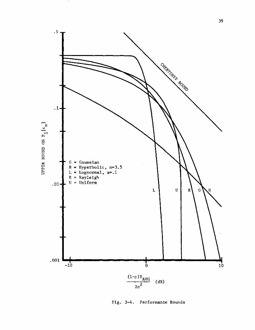
These results are presented in Fig. 3-4 for the five two-sided p.d.f.s

of Table 3.1. A comparison of the bounds to performance results for

specific signal sets is presented in Chapter 4.

TABLE 3.1

NORMALIZED PROBABILITY DENSITY FUNCTIONS

Distribution Density Function PN(n) Restrictions

Gaussian1 . 2

- exp[-n /2];Z;

RayleighInl exp[-n

2](Two-Sided)

Lognormal 1 [_ [ln~3 "2]2 ] a > a(Two-Sided) exp

2;Z; a Inl

Uniform 1Inl < 13--

ill

Hyperbolic 1 (m-l) [(m-2) (m-3)] (m-l)/2 3 < m < 6(Two-Sided) - -

12 [/(m-2) (m-3) + 12 Inl]m

39

.5

.1

.01

G = GaussianH = Hyperbolic, m=3.5L Lognormal, 0=.1R RayleighU = Uniform

L U

.001 ...+------------+--..- .......--..- .....-10 o 10

(dB)

Fig. 3-4. Performance Bounds

CHAPTER 4

SPECIFIC PERFORMANCE RESULTS

Waveforms are chosen for the GIN (Unique Waveform) model and used

to calculate numerical performance results, illustrate the effect of

the weighting factor p.d.f., compare performances of various signal

sets, and study the tightness of the bound curves derived in Chapter 3.

4.1 GENERALIZED IMPULSE NOISE WAVEFORMS

The determination of the impulse noise waveforms present in a

communication system requires extensive measurements and the use of

special test equipment. Two specific waveforms, a decaying exponen­

tial and an exponentially-decaying sinusoid, are selected for closer

examination, based upon the measurements on the simulated Space Shut­

tle data bus [33] and the unit-impulse-response conjecture proposed

in Section 2.1.

4.1.1 Decaying Exponential

The decaying exponential is the unit-impulse response of a

channel modeled by a first-order Butterworth transfer function.

In order to conserve computer time, the waveform is truncated at

TF seconds. The expression for the truncated, unit-energy wave­

form is

40

f(t) A exp(-bt), o < t < TF (4.1)

41

where the decay rate depends on the time constant (lib) and for the

assumption of unit energy

A =~ l-:-l

_-..::2.....b-:--:-:-----:-V - exp(-2bTF)(4.2)

Usually the waveform duration (TF) is chosen to equal several time

constants. Waveforms are presented in Fig. 4-1 for time constant

and duration values that are used in obtaining the performance

results of Section 4.2. A unit-energy pulse is shown for compari-

son. It follows from (4.2) that the noise waveforms have larger

peak values as the time constant and duration are decreased.

4.1.2 Exponentially-Decaying Sinusoid

The second unit-energy waveform selected is the truncated,

exponentially-decaying sinusoid, i.e.,

f(t) C sin(2nf t) exp(-dt).o

o < t < TF (4.3)

It is assumed that the waveform duration is a multiple of the

sinusoid period, i.e.,

TF nf

on = 1,2, ... (4.4)

Hence, to preserve the unit-energy assumption it follows that

150

1m

s

4m

s

o30

120

lib

0.1

ms

,-...

90TF

1m

s:> '-"

~ 0 ;::l H H ~ ~

60

o1

23

4

TIM

E(m

s)

Fig

.4

-1.

Decay

ing

-Ex

po

nen

tial

Wav

efo

rms

C = 1TIf

o[1 - exp(-2dTF)]

43

(4.5)

The values for d,f , and TF can be chosen to model both basebando

channels without dc response and band-pass channels.

4.2 PERFORMANCE RESULTS FOR DECAYING EXPONENTIAL

Several sets of performance results are presented and comparisons

made to illustrate the effect of the weighting factor p.d.f., signal

set, and noise waveform. Results for the five signal sets shown in

Fig. 4-2 with alms bit time are obtained using the Fortran-IV com-

puter program GINIMP which is described in Appendix C. A frequency

of 1 kHz is used for the ASK and PSK signal sets. For FSK, a fre-

quency of 1 kHz is used for sl (t) while 2 kHz is used for sO(t). The

program requires approximately 2.5 minutes of IBM System/360 computer

time for each overlapped data bit and ENP value analyzed; consequently,

only three or four points are computed for each case and a smooth

curve drawn through the points. to obtain the performance curve. Bound

curves are displayed for comparison with the performance results.

These bounds are obtained after multiplying the Pl[Em] value obtained

from Fig. 3-4 by the number of data bits that the noise waveform can

possibly overlap. Although the bounds are not tight, they do have the

general shape of the actual performance curves and can be obtained with-

out knowledge of the noise waveform.

+v

a

+v

ONE

(a) UNIPOLAR NRZ

-v

(b) POLAR NRZ

ZERO

44

a

+v

a

+v

a

(c) ASK

(d) PSK

(e) FSK

Fig. 4-2. Five Typical Signal Sets

45

4.2.1 Weighting Factor Distribution

The effect of changing the weighting factor (I) p.d.f. is

demonstrated in Fig. 4-3. Unipolar signaling and the decaying-

exponential noise waveform with a 0.2 ms time constant are used

to obtain performance results for the five weighting factor p.d.f.s

of Table 3.1. The Gaussian, Rayleigh, and uniform distributions

yield results which are approximately equal. The results for the

lognormal and hyperbolic distributions were obtained for parameter

values a=O.l and m=3.5, respectively. The parameter value controls

the shape of these p.d.f.s and should have a corresponding control

in the shape of the error performance curves. Results for typical

parameter values in these distributions and an idealized impulse

waveform have been presented by Houts & Moore [11]. The Gaussian

p.d.f is selected as being typical and is used exclusively in

determining the remaining performance results.

4.2.2 Waveform Time Constant

The effect of changing the decaying-exponential time constant

is studied in Fig. 4-4 for Unipolar signaling and a Gaussian p.d.f.

It was necessary to increase the waveform duration (TF) for the

1 ms time constant in order to calculate its true impact on the

data. The expected number of bit errors increases with the time

constant, which is intuitively satisfying since for large time

constants the noise waveform more closely approximates the Unipolar

1

46

.1

.01

.001

G = GaussianH = Hyperbolic, m=3.5L = Lognormal, a=.lR = RayleighU = Uniform

L U R

-50 -40

ENP (dB)

-30 -20

Fig. 4-3. Effect of Weighting Factor P.D.F. on UnipolarSignaling in the Presence of Decaying-ExponentialNoise with 0.2 ms Time Constant

47

1

,.....,z.......,>:<:l

.. .1V)p:::

~p:::>:<:l

E-l lIb =H TFP=l =~

0p:::>:<:l

~z lIb 0.2 ros= 1A = ros>:<:l TF = 1 ros 4E-l IDSU>:<:l

~>:<:l

.01

-50 -40

ENP (dB)

-30 -20

Fig. 4-4. Effect of Decaying-Exponential Waveform TimeConstant on Performance of Unipolar Signaling

48

waveform. Hence, the correlation receiver would be more likely to

mistake the noise for a signal bit.

A similar presentation is made in Fig. 4-5 for ASK signaling.

Note that for ENP values greater than -43 dB, the curve for the 1

ms time constant indicates a lower error rate than the curves for

the shorter time constants. A plausible explanation for this

apparent contradiction to the trend is the lower peak cross-

correlation which results from the unit-energy noise waveforms.

The peak value of the noise must decrease as the time constant

and/or duration are increased. As the peak value decreases, the

minimum weighting factor, I , , must increase before an errormln

occurs; however, the probability of I assuming values greater

than the new I, is smaller, thus the error rate decreases. Themln

effect of the peak values in the correlation function becomes evi-

dent as the ENP value inGreases. The bound curves presented in

Figs. 4-4 and 4-5 are obtained by doubling (3.69); hence, they

only apply to the noise waveforms of 1 ms duration. The bound

for the 4 ms waveform appears in Fig. 4-10.

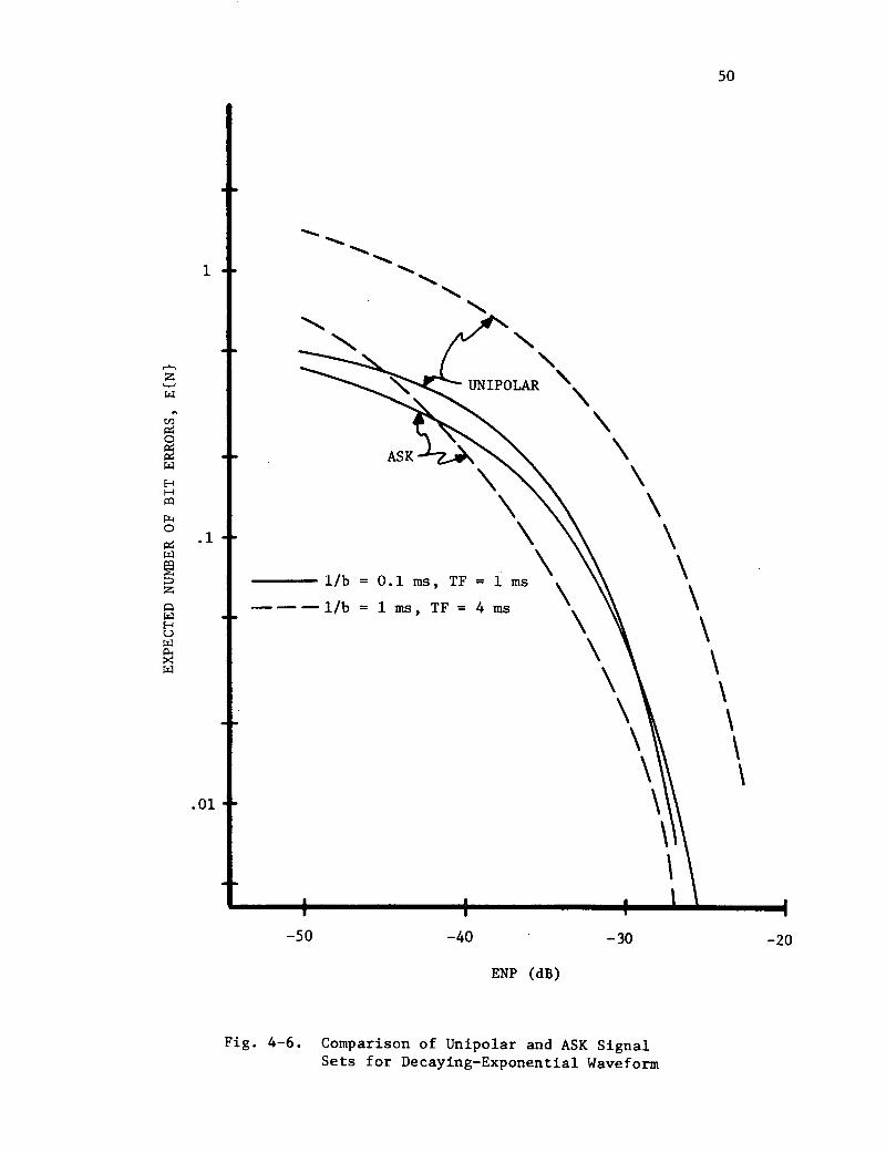
The'relative performance of the Unipolar and ASK signal sets

is dependent on the time constant of the decaying-exponential noise

waveform, as illustrated in Fig. 4-6. The ASK performance shows a

5 to 10 dB improvement for the larger time constant. This reflects

the generally lower ASK-noise crosscorrelation values (including

peak values). For the 0.1 ms time constant, the Unipolar-noise

crosscorrelation function (including peaks) is slightly larger than

for ASK signaling, which explains the better performance of ASK at

1 __ .,t--- Bound (TF= 1 IDS)

=

= 0.2 IDS

= 1 IDS

,......., .1lIb 1=z....... TF = 4

~

~

enp::0gl~

HHr:Q

~0

p::~r:Q

?5z~~H .01u~~:<~

.001

49

-50 -40

ENP (dB)

-30 -20

Fig. 4-5. Performance of ASK Signaling for VariousDecaying-Exponential Time Constants

1

.1

.01

---lib =

---lib =

-50

0.1 ms, TF =1 ms, TF = 4 ms

-40

50

"-"-",

"\\\\\\\\\\\\

-30 -20

ENP (dB)

Fig. 4-6. Comparison of Unipolar and ASK SignalSets for Decaying-Exponential Waveform

51

low ENP values. However, the ASK signal set has a larger peak value

than the Unipolar set, which is reflected in the performance equations

of (3.57) and (3.58), and accounts for the crossover of the curves

for larger ENP values.

4.2.3 Signal Set

An error performance comparison for five signal sets is shown

in Fig. 4-7 for a Gaussian p.d.f. description of I and the decaying­

exponential noise waveform with a 0.2 ms time constant. Several

conclusions can be made from a study of these results. The error

performance of Polar (or PSK) signaling exhibits a 3 dB improvement

in ENP value over that of Unipolar (or ASK). This result agrees

with that observed for AWG noise. Conversely, it is apparent that

a difference exists in the performances of Unipolar and ASK signals

(or Polar and PSK) which is not present with AWG noise. Furthermore,

the FSK signal set performance appears to approach that of ASK for

large ENP values, which contradicts the AWG noise results for which

the signal sets have equal performance. Furthermore, for ENP values

below -33 dB the FSK error rate becomes less than that for PSK.

Although the FSK-noise crosscorrelation is generally less than that

obtained with the single sinusoid used for ASK and PSK, it does have

slightly larger peak values. This explains the change in the relative

performance of FSK as the ENP value increases.

The bound curves in Fig. 4-7 are upper bounds and it appears that

the bound for p = -1, i.e., Polar or PSK signaling, could be used for

all five signal sets. However, this conclusion is not valid, as it

52

1

.1,.......z.....,w

..tf)p:::0gjW

HHl:Q

~0p:::w

~Z

0 .01wHUW

~W

forand PSK

Bound forUNIPOLAR,

ASK, andFSK

.001 ..--...------+------~~-.................-50 -40

ENP (dB)

-30 -20

Fig. 4-7. Comparison of Five Signal Sets for Decaying­Exponential Waveform with 0.2 ms Time Constant

53

applies only for this particular set of assumptions regarding noise

waveform, time constant, and weighting factor p.d.f.

4.3 PERFORMANCE RESULTS FOR EXPONENTIALLY-DECAYING SINUSOID

The effect of changing the noise waveform is demonstrated by

considering the exponentially-decaying sinusoid of (4.3). Unipolar

and ASK signal sets are compared in Fig. 4-8 for two values of the

noise time constant and a Gaussian p.d.f. The higher error rate for

ASK is explained by the larger correlation between the signal and

noise waveforms. Similarly, the improvement experienced by Unipolar

signaling as the time constapt is increased is due to the decreased

correlation between signal and noise. The relative performance of

the two ASK curves reflects a generally larger crosscorrelation with

the noise for the 2 ms time constant, but a larger peak cross­

correlation for the 1 ms time constant.

A comparison of the five signal sets is presented in Fig. 4-9

for the exponentially-decaying sinusoidal noise waveform with a time

constant of 1 ms. These results indicate the same 3 dB improvement

of Polar over Unipolar and PSK over ASK as is obtained with an AWG

noise assumption. The FSK performance is almost the same as the PSK

over the range of ENP values shown, and thereby differs from the 3 dB

differential for AWG noise results. The performance difference

between Unipolar and ASK also contrasts with AWG results.

54

1

,.....,z.......~

..(J)

IX:

~~

E-t .1 \HP:l

~ \0

IX:~ lId = 1 ms, TF "" 4ms \~z --- lId = 2 ms, TF = 4ms

\Cl~E-t \u~

~ \~

\.01

\\\\

-50 -40 -30 -20

ENP (dB)

Fig. 4-8. Comparison of Unipolar and ASK Signal Setsfor Exponentially-Decaying Sinusoid

10

1

,......,z.......1il

U)p::0

~1il

HHIX)

~0p::1il

~z .101ilHU1il

~1il

.01

55

-50 -40

ENP (dB)

-30

Fig. 4-9. Comparison of Five Signal Sets for Exponentially­Decaying Sinusoid with 1 ms Time Constant

56

4.4 EFFECT OF SIGNAL AND NOISE CORRELATION

The performances of Unipolar and ASK signals are compared in

Fig. 4-10 using both the decaying-exponential and the exponentially­

decaying-sinusoidal noise waveforms with the same time constant and

a Gaussian p.d.f. for I. It is noted that the performance of ASK

with the decaying-exponential noise is approximately equal to that

of Unipolar with exponentially-decaying-sinusoidal noise. This is

reasonable, since in both cases the signal and noise crosscorrelation

are essentially equal. The larger peak value of the ASK signal set

dictates the crossover in the relative performances as the ENP value

increases. When the noise waveforms are interchanged, the ASK sig­

nal set has a small advantage over Unipolar, although both perfor­

mances are inferior to the aforementioned combinations.

4.5 COMPARISON TO RESULTS FROM THE LITERATURE

The relative performance of various signal sets has received

some attention in the literature. Usually, the comparisons are

between signaling methods that utilize a carrier, e.g., ASK, PSK,

or FSK. For idealized impulse noise and coherent demodulation,

it has been shown by Ziemer [10] and Houts & Moore [11] that PSK

exhibits a 3 dB improvement over ASK. Houts and Moore have also

shown that the performance of FSK differs from ASK. Engels [24]

and Bennett & Davey [38] have used more realistic noise models to

show that PSK performs better than FSK. Experimental measurements

reported by Bodonyi [23] have shown the presence of crossovers in

57

Bound (TF=4 ms)

UNIPOLAR

"""""\\\\\\\\\\\

-- -- -- Decaying Exponentia1

------- Exponentially-Decaying Sinusoid

1

.1

.01

-50 -40 -30 -20

ENP (dB)

Fig. 4-10. Comparison of Unipolar and ASK Signal Setsfor Waveforms with 1 rns Time Constants

the performance curves for noncoherent FSK and coherent PSK sig­

naling techniques. However, for large SNR values it appears that

PSK has an advantage. These results for carrier systems appear

to support Bennett & Davey's hypothesis that the relative error

rates of data transmission systems can be determined for nearly

all noise environments by comparing performances in the presence

of AWG noise.

Most of the above results are consistent with the results

of Sections 4.2, 4.3 and 4.4. However, the performances of the

On-Off, Binary Antipodal and Orthogonal signaling methods were

shown to be dependent on the signal-set basis function, e.g.,

pulse or sinusoid. This represents a major exception to the

AWG-relative-performance hypothesis proposed by Bennett & Davey.

This discrepancy is caused by the error performance for impulse

noise being dependent upon the signal-to-noise correlation,

whereas AWG noise is uncorrelated with all signal sets. New

conclusions have also been obtained. The 3 dB improvement of

PSK over ASK has been established for the GIN (Unique Waveform)

model, and for the conditions investigated, the FSK signal set

can perform better than PSK for low ENP values. Similarly, a

study of pulse signaling has revealed that the 3 dB advantage

exist for Polar over Unipolar.

58

CHAPTER 5

METHODS FOR IMPROVING RECEIVER PERFORMANCE

The linear correlation receiver does not represent the optimum

receiver for impulse noise corrupted signals. In fact, a variety of

methods have been proposed for improving the receiver design. A sur­

vey of these recommendations is presented in Section 5.1, after which

a specific improvement method is selected for analysis and the perfor­

mance results are compared to the linear correlation receiver. Many

factors other than the receiver design can affect the performance of

a digital system, e.g., noise source proximity, system shielding,

ground loops, etc. Such factors are not considered here.

5.1 SURVEY OF RECOMMENDATIONS FOR IMPROVED RECEIVER DESIGNS

The topic of designing receivers for impulse-noise corrupted

signals has not received extensive treatment in the literature.

However, several intuitively-motivated techniques have been reported

which employ theoretical and/or experimental procedures. Generally,

the proposed improvements attempt to counteract either the large

amplitude or aperiodic nature o£ the impulse noise and will be clas­

sified as either amp1itude- or time-based modifications to existing

receivers.

The amplitude-based modifications act to suppress the large

amplitude excursions of the impulse noise by including a nonlinear

59

60

device in the receiver. As discussed in Section 1.2, Snyder [31] and

Rappaport & Kurz [32] have used the likelihood ratio to investigate opti­

mum receivers for specific impulse noise models. Each design resulted

in the use of a nonlinear device to suppress large amplitude excursions

in conjunction with a linear receiver. The specification of the non­

linear device depends on the noise statistics and must be changed if

the noise description changes. Sub-optimum receiver designs using

nonlinear devices have been proposed with either intuitive or empiri-

cal justification. Specifically, several authors [13,26,27,39,40]

have proposed clipping devices which limit the maximum magnitude of

the received signal. Another suggestion [29] is to use a blanking

device which has a zero output when the input signal exceeds specified

positive and negative thresholds. It has been postulated that the

reduction in noise power achieved through the use of clipping or blank­

ing devices yields improved error performance; however, there is no

such guarantee because of the possibility of improving the signal-to­

noise crosscorrelation. Bello & Esposito [12] have reported the per­

formance improvement obtained using a clipping device with PSK signal­

ing and an atmospheric noise nodel. They assumed that the amplitude

of the noise was much greater than that of the data signal.

The time-based modifications exploit the aperiodic and frequency

spectrum properties of the impulse noise. Examples of this technique

are the smearing-desmearing [30] and swept-frequency-modulation [41,42]

systems. These systems use a special modulator or a filter to destroy

the phase relationship of the components in the transmitted signal. At

the receiver the inverse of this operation is performed which yields

61

the original phase relationship for the data signal, but destroys the

phase relationship of the channel noise components. These techniques

have not been employed extensively because of their poor performance [43],

One possible explanation for the poor performance is that the true char-

acteristics of impulse noise are not represented by a model where ampli-

tude peaks are caused by a phase relationship of noise components.

Another time-based modification uses a pulse-width discriminator [28]

to decide if the received signals are noise or data pulses. Those that

qualify as data bits produce fixed-width pulses at the output of the

discriminator. This system can only be effective if the time duration

of the noise waveforms are short, compared to the data bit.

5.2 PERFORMANCE ANALYSIS FOR A NONLINEAR CORRELATION RECEIVER

The error performance of the system shown in Fig. 5-1 is deter-

mined using the general approach developed in Chapter 3. The first

step is to find the conditional decision statistic, Dj , for the mth

bit, viz.,

mTb

~ {Sj(t) + n(t)}o [sl(t) - sa(t)] dt - C ,

(m-l)Tb

(5.1)

where { }o represents the operation performed by the nonlinear device.

Equation 5.1 can be changed into the form of (3.16). First, s,(t) isJ

added and subtracted to the { }o term and the following notation is

introduced.

(5.2)

m.

Sj(t

)..

Lre

t)0

MES

SAG

EJ

-TR

AN

SMIT

TER

..N

ON

LIN

EAR

r(t

)..

CORR

ELA

TOR

-SO

URCE

--

-D

EVIC

E-

-U

net)

Fig

.5

-1.

Dig

ital

Sys

tem

wit

hN

on

lin

ear

Co

rrela

tio

nR

ecei

ver

m

63

Incorporating (5.2) into (5.1) and dropping the limits of integration

gives

(5.3)

where C. is defined by (3.17). Assuming noise which is represented byJ

the GIN (Unique Waveform) model and ignoring the possibility of more

than one burst in a bit interval yields

j I J{ }oo (n (NB=l) = I f(t-T) [sl (t) - So t)] dt - Cj

.

The normalized random variable N=I/cr can be introduced by defining

another nonlinear operation, namely,

(5.4)

cr {N f(t_T)}oOO = {cr(I/cr) f(t_T)}oO .

Thus

(5.5)

nj I (NB=l) (5.6)

Factoring the peak voltage V from the signal set and defining

V F. (N, T)J

yields

(5.7)

nj I (NB=l) cr V F.(N,T) - C.J J

(5.8)

64

Following the procedure used in obtaining (3.32) the normalized proba-

bility of bit error can be written using (5.8) as

Pl[t: 1m.]m J

= P[(-l)j F.(N,T) > (-l)j C./(aV)] .J J

(5.9)

Alternatively, (5.9) can be represented as

l\[t:m1mj ] = JIP[(-l)j Fj(n,T) > (-l)j cj/(av) IN=n,T=T]

n T

or

(5.10)

(5.11)

where R. designates the region of Nand T such that the inequalityJ

established on F.(n,T) in (5.10) holds. Assuming that T is uniformlyJ

distributed over the bit interval and integrating over T yields

Pl[t: 1m.]m J

00

J TR(n)PN(n) dn ,

NP

(5.12 )

where the time range TR(n) equals zero for -Nn<n<Np '

The nonlinear device must be specified before numerical results can

be obtained. The limiter model of Fig. 5-2 represents an extension of

the clipping and blanking concepts discussed in Section 5.1 and is use~

by the computer program LIMITER, which is described in Appendix D, to

determine the error performance given by (5.12). Values for a and ap n

vout

Fig. 5-2. Limiter Model

65

66

correspond to the magnitudes of the peak positive and negative signal

set voltages, respectively. For ASK, PSK, FSK and Polar signal sets

a = a , while for Unipolar and other one-polarity signal sets, a =0.p n n

The values of 6 and 6 are parameters specified by the user, thusp n

either a specific limiter can be modeled or the values changed to

determine their effect on the error performance.

5.3 COMPARISON OF LINEAR AND NONLINEAR CORRELATION RECEIVERS

Performance results for the linear and nonlinear correlation

receivers are compared for several signal sets. The results for the

nonlinear device were obtained by running the LIMITER program on the

UNIVAC-ll08 computer. Each value calculated required approximately

10 minutes of CPU time for each data bit analyzed, i.e., 40 minutes

of computer time was required to obtain one point if the noise wave-

form overlapped four data bits. For this reason, a comprehensive

study of signal sets, weighting factor p.d.f. and noise waveform param-

eters was not attempted. The results presented assumed a Gaussian

p.d.f. for the weighting factor.

The error performance curves presented in Fig. 5-3 illustrate the

effect of changing the clip levels 6 and 6 •n p When 6 =a and 6 =0, ap p n

performance improvement of approximately 6 dB is obtained in comparison

with the case where 6 =6 =a. This is intuitively satisfying, sincep n p

setting 6 =0 is a logical choice for Unipolar signaling. For both setsn

of clip-level values the performance improvement over the linear corre-

lation receiver decreases as the ENP value increases. However, at a

-310 error rate there is still an impressive 5 dB improvement over the

671

Linear Receiver

8 8 =n p

,......, .1z......,~

~

CIlp::0p::p::~

E-tHP=l

~0p::

8 0~

~n

8p exz p0~E-t .01u~

~~

.001-50 -40 -30 -20

ENP (dB)

Fig. 5-3. Effect of Nonlinear Receiver on Unipolar SignalPerformance in the Presence of Decaying-ExponentialNoise with a 0.2 ms Time Constant

Fig. 5-6 for two versions of the limiter.

68

linear receiver for the case when S =a and S =0. It is reasonablep p n

to assume that the performance improvement decreases as ENP increases

since the data signal begins to dominate the noise and the clipping

device will have less overall effect. A similar conclusion is obtained

from a study of Fig. 5-4 for ASK signaling and the decaying-exponential

noise waveform. The clip levels correspond to the peak voltage of the

signal set, i.e., S =S =a. As before, the performance improvementp n p

decreases as the ENP value increases. It was shown in Chapter 4 that

the Unipolar signaling performance was poorer than ASK when linear cor-

relation detection was used in the presence of decaying-exponential

noise. This disparity was attributed to the higher cross correlation

between the Unipolar signal and the noise. However, a comparison of

the error performances shown in Figs. 5-3 and 5-4 indicates that the

Unipolar signal performs better than ASK when the limiter is inserted,

at least for the chosen values of Sand S .p n

The exponentially-decaying sinusoidal noise waveform with a 2 ms

time constant was used to investigate the relative performance of ASK

and PSK signaling. A comparison of ASK signaling performances for the

linear and nonlinear receivers is shown in Fig. 5-5. The clip levels

were not chosen to equal the peak signal value, instead they correspond

to the rms value, i.e., S =S =a /1:2. Although for low ENP values ap n p

very small improvement is obtained, the curves have converged for an

ENP greater than -30 dB. The PSK signaling performance is shown in

When S =S =a /1:2, the per­p n p

formance is actually poorer than it was for a linear correlation detec-

tor. It is evident that improved performance can be obtained through a

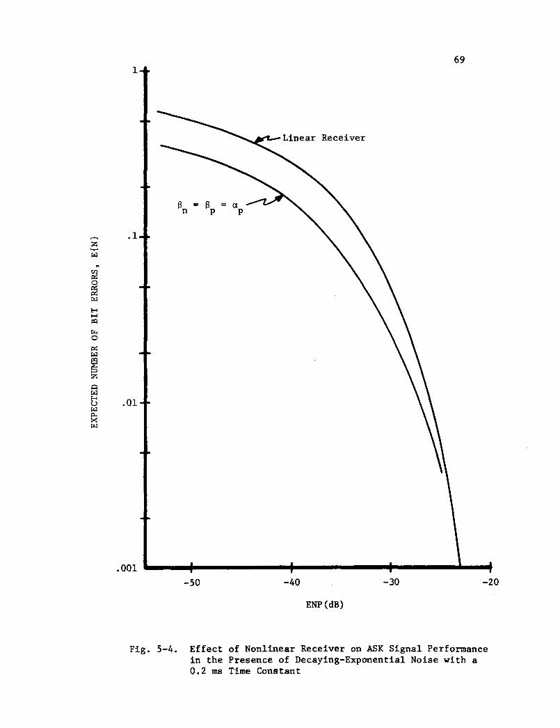
691

Linear Receiver

B = B =n p

,....., .1z......r>:l

tilp::0

~r>:l

Ht-t!Xl

~0p::r>:l

~Z

Ar>:lH .01ur>:l

~r>:l

.001

-50 -40 -30 -20

ENP (dB)

Fig. 5-4. Effect of Nonlinear Receiver on ASK Signal Performancein the Presence of Decaying-Exponential Noise with a0.2 rna Time Constant

70

Linear Receiver1

..rIl;~

HHJ:l:l

~ ..1oc:x:~

~zo~HU~

~~

.01

-50 -40

ENP (dB)

-30 -20

Fig. 5-5. Effect of Nonlinear Receiver on ASK Signal Performancein the Presence of Exponentia11y-Decaying-Sinusoida1Noise with a 2 ms Time Constant

71

8 = 8 =n p

.1

.01

-50 -40

ENP (dB)

Linear Receiver

-30 -20

Fig. 5-6. Effect of Nonlinear Receiver on PSK Signal Performancein the Presence of Exponentially-Decaying-SinusoidalNoise with a 2 rns Time Constant

72

more logical choice of clip levels, i.e., S =8 =a ; however, the effectp n p

is minimal for either set of clip levels. Consequently, with a limiter,

PSK does not possess the full 3 dB advantage over ASK which was present

for linear correlation detection.

The results presented in this section indicate that error perfor-

mance can be improved by the proper choice of clip levels in the non-

linear receiver. The improvement obtained by using the limiter would

probably become more pronounced as the noise time constant decreases,

since the peak noise voltage increases to meet the unit-energy assump-

tion for the basic waveform f(t).

CHAPTER 6

CONCLUSIONS AND RECOMMENDATIONS

6.1 CONCLUSIONS

The generalized impulse noise (GIN) model can approximate the

noise burst structure observed in many digital systems provided the

average burst rate, expected number of waveforms per burst, sample

function ensembles associated with the burst, and the weighting

factor p.d.f. can be obtained. A specialized model, the GIN (Unique

Waveform) model, is readily obtained by assuming that each noise burst

contains a randomly weighted version of the same basic waveform. It

has been shown that the power-density spectrum for this specialized

model is not white because of the dependence on the noise waveform.

The GIN (Unique Waveform) model is used to determine the error

performance equations for a correlation receiver. These results

express the expected number of bit errors per noise burst as a func­

tion of the following parameters: (1) energy-to-noise parameter (ENP)

of (2.12), (2) noise amp1itude-weighting-factor p.d.f., (3) signa1­

set correlation coefficient, and (4) a time range function which

depends on cross correlation between the signal-set basis functions

and the noise waveform. The performance analysis for the GIN (Unique

Waveform) model can be extended to the general model.

Comparison of the performance results for impulse and additive

white Gaussian (AWG) noise reveals two major differences. For

73

74

impulse noise, Orthogonal signaling does not yield the same error

performance as On-Off signaling with the same average energy. Also,

the choice of the signal-set basis functions has an effect on the

performance. These conclusions are supported by the dependence of

impulse noise performance results on the correlation between the

signal and noise waveforms. A conclusion which agrees with the MvG

result is that Antipodal signaling has a 3 dB advantage over On~Off

signaling.

The error performance can be upper bounded by equations which

depend on the average signal energy, signal-set correlation coef­

ficient, plus the noise weighting-factor variance and p.d.f. Spe­

cifically, the bounds do not depend on the signal-set basis functions

or the noise waveform. Another upper bound, which is also independent

of the weighting factor p.d.f., is formed by applying Chebyshev's

inequality to the previous bound. It has been shown that for impulse

noise the linear correlation receiver is not optimum, i.e., the proba­

bility of error is not minimized. This conclusion is supported by the

dependence of the performance equations on the signal and noise cross­

correlation. One method for improving the error performance is to

insert an amplitude-dependent limiter, i.e., a nonlinear device, prior

to the receiver input. It was shown that the error performance is

dependent upon the choice of parameters used to specify the limiter.

6.2 RECOMMENDATIONS FOR FURTHER STUDY

Further work can be performed in several areas of this inves­

tigation. The relationship between signal-to-noise ratio (SNR) and

75

ENP has been established only for white Gaussian noise and idealized

impulse noise. It would aid the comparison of results if the param-

eters were related for a bandlimited channel and the GIN model. This

study has concentrated on the analysis of the correlation receiver,

but an investigation of sampling receivers could be performed as sug-

gested by the procedure of Chapter 2. The extension of the nonlinear

receiver designs of Chapter 5 to an optimum receiver for impulse noise

offers an opportunity for a significant contribution.

Although the bounds of Chapter 3 are useful, other techniques

should be investigated in an attempt to improve the tightness of the

bounds. It might be possible to approximate the error performance of

the GIN (Single Ensemble) model by using an average waveform G(t) which

is obtained by averaging over the sample functions in the ensemble.

For example, the error expression of (3.7) might become,

NE

E{N} = E{NG} ~ E{NlIGk(t)} P[Gk(t)] ~ E{NG} E{Nl!C(t)}

k=l

where

NE

~ Gk(t) P[Gk(t)]

k=l

(6.1)

(6.2)

Once G(t) is obtained, the evaluation of E{Nllc(t)} is equivalent to

the techniques developed herein for the unique waveform model. Finally,

the derivation of upper bounds for various nonlinear correlation receiv-

ers would reduce the computer time required to obtain specific results.

APPENDIX A

DERIVATION OF POWER-DENSITY SPECTRUM AND PROBABILITY DENSITYFUNCTIONS FOR THE GIN (UNIQUE WAVEFORM) MODEL

In order to characterize the GIN (Unique Waveform) model it is

helpful to specify both the noise power-density spectrum and ampli-

tude probability density function (p.d.f.). These expressions are

derived in the following sections. In particular, two p.d.f. descrip-

tions are obtained for the noise model. The first p.d.f. is based on

the assumption that no more than one noise burst occurs in time T tn

and the second results from using a Poisson distribution to model the

number of noise bursts.

A.I POWER-DENSITY SPECTRUM

The power-density spectrum can be determined from the expression

for the average power, PAVG ' by

(A. I)

where T is the duration time of the noise and the expected value E{ }n

is taken with respect to all of the random variables involved in des crib-

ing the noise process. The first step is to apply Parseval's theorem,

viz. ,

76

77

1T

n

1T

n

00

(A.2)

where N(f) is the Fourier transform of a sample function from the nqise

process. For the GIN (Unique Waveform) model of (2.7),

NB

N(f) = l: Ik

F(f)e-j2nfTk

k=l

where F(f) is the Fourier transform of f(t). Thus

(A.3)

IN(f) 12 N(f).N*(f)

NB NB

~ ~ IkIkIF(f)12 e-j2nf(Tk-Ti)

k=l i=l

(A.4)

Substituting (A.2) into (A.l) and interchanging the order of integra-

tion and expectation gives

00

PAVG = in ~ E{IN(f) 12

} df-00

The expected value of IN(f)!2 with respect to I is given by

(A.5)

NB NB

Er {IN(f)12

} = L L Er {IkIi } IF(f)12

k=l i=l

-j21Tf(Tk-T·)e ~ (A.6)

For the case where I k and Ii are zero-mean independent random variables,

it follows that

the weighting factor variance.

then (A.6) becomes

where 0ik = 0 if i i k and o~ is

is a constant 02 for all bursts,

(A.7)

78

Taking the expected value of (A.7) with respect to NB yields

For a process where ENB{NB} = vBTn (e.g., a Poisson process with

average rate vB) the average power expression of (A.5) becomes,

00

~ vBo2

IF(f) 12

df_00

(A.9)

It follows from (A.9) that the one-sided power-density spectrum is

S (f)n

(A.IO)

This result can be extended to the GIN (Single Function) model of

(2.6) by replacing f(t) with the sample function Gk(t) and taking

the expected value with respect to the type of waveform. The result

is

S (f)n

NE

L 1~{Gk(t)}12 P[Gk(t)]

k=l

(A. H)

where ~{Gk(t)} is the Fourier transform of Gk(t).

A.2 PROBABILITY DENSITY FUNCTIONS

The GIN (Unique Waveform) model is used in determining p (a),n

the amplitude p.d.f. for impulse noise. Two random variable models

are examined for NB, the number of bursts that occur in time T .n

79

The procedure used in the derivation is similar to that employed by

Rice [35], Middleton [36], and Ziemer [10]. The characteristic func-

tion M(u) is determined first and the noise p.d.f. is obtained through

an integral transform.

A.2.1 Basic Form of Characteristic Function

The characteristic function M(u) can be expressed in terms of

the number of noise bursts that occur, viz.,

00

where

M(u) = L M(u INB) P [NB]

NB=O

(A.12)

NB

E{~XP [ju L Xkf(t-Tk)]}

k=l

(A.13)

It is assumed that the random variables I k and Tk are statistically

independent and that I k (or Tk ) is independent of Ij

(or Tj), j # k.

It is further assumed that the p.d.f. descriptions for the weighting

factor and occurrence time do not change between bursts. Hence, the

subscripts are dropped and

M(uINB) = [E{ejuIf(t-T)}]NB

The expected value is given by

(A.14)

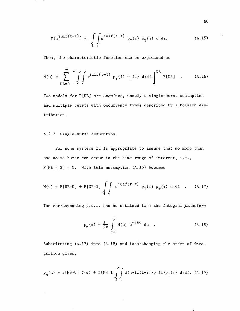
]' uIf (t-T) JJe]' uif (t-T)E{e } = PI(i) PT(T) dTdi.

i T

Thus, the characteristic function can be expressed as

00

80

(A. IS)

M(u) L [JJejuif(t-T)

NB=O i T

(A.16)

Two models for P[NB] are examined, namely a single-burst assumption

and multiple bursts with occurrence times descr~bed by a Poisson dis-

tribution.

A.2.2 Single-Burst Assumption

For some systems it is appropriate to assume that no more than

one noise burst can occur in the time range of interest, i.e.,

P[NB ~ 2] = O. With this assumption (A.16) becomes

M(u) = P[NB=O] + P[NB=I] JJi T

j uif ( t - T) ( . ) () d d'e PI 1 PT TTl (A.I7)

The corresponding p.d.f. can be obtained from the integral transform

00

Pn(a) = ~TI JM(u) e-jua

du_00

(A.18)

Substituting (A.17) into (A.18) and interchanging the order of inte-

gration gives,

p (a)n P[NB=O] o(a) + P[NB=ll!Jo(a-if(t-T))Pr(i)PT(T) dTdi. (A.19)

i T

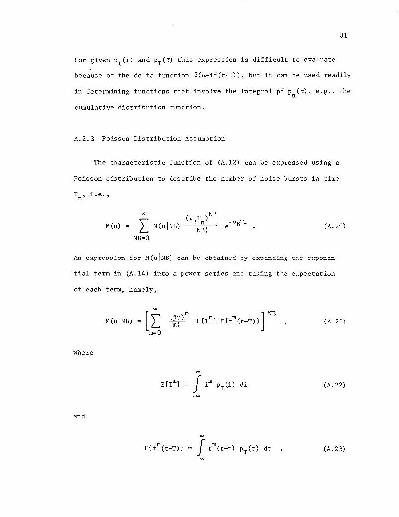
81

For given Pr(i) and PT(T) this expression is difficult to evaluate

because of the delta function o(a-if(t-T», but it can be used readily

in determining functions that involve the integral pf p (a), e.g., then

cumulative distribution function.

A.2.3 Poisson Distribution Assumption

The characteristic function of (A.12) can be expressed using a

Poisson distribution to describe the number of noise bursts in time

T, i.e.,n

M(u)

00

LNB=O

-VBTen. (A.20)

An expression for M(uINB) can be obtained by expanding the exponen~

tial term in (A.14) into a power series and taking the expectation

of each term, namely,

00

[L (ju)~ rM(u!NB) E{rm} E{fm(t-T)}m!m=O

where

00

E{rm} Jim

Pr(i) di_00

and

00

E{fm(t-T)} Jfm(t-T) PT(T) dT_00

(A. 21)

(A. 22)

(A.23)

82

If the burst occurrence times are uniformly distributed over T , thenn

1=-

Tn

mf (t-T) dT (A.24)

Substituting (A.24) and (A.21) into (A.20), gives

00 00 T

L-vBT

[VB L c )mE{Im} In rM(u)

e n JU fm( t-T) dT . (A.25)NB~ m:

NB=O m=O 0

Letting

T

A E{Im} In mm vB f (t-T) dT

0

then

00 00

M(u) = e-VBTn LN~: [L A (ju)m r"m m~

NB=O m=O

00

-vBT [L A (j u)m ]e n exp m m:m=O

00

exp [L A (j u) m ]m: .m

m=l

(A.26)

(A.27)

When I is symmetrically distributed about a zero mean, it follows that

E{I} 0 and from (A.26) that Al = O. The p.d.f. for the noise can be

determined from the transform relation of (A.18). It follows that

00

Pn(a) = ~TI Jexp[-jUa-u2

A2/2]_00

(A.28)

83

A series solution can be obtained by a two-step procedure, namely

replace the second exponential by

00

exp [Lm=3

>.. (j u) m ]m m: 1 +

00

m=3

m >..Z, (j u) + --.1. (. )6I\m m: 72 JU + ... (A.Z9)

and perform a term-by-term integration using the integral relation

00J(ju)n eXP[-jua-uZ>..z/Z] du_00

(_l)n ~ dn

exp[-aZ/2A.z ] . (A. 30)y~ dan

The derivation of (A. 30) is presented in Section A.Z.4. The p.d.f.

becomes

-Z

p (a) 1 1jJ(0) (x) >"iz 1jJ (3) (x)= --3:n

~[A A -5/2

1jJ(4)(x) +>..Z>.. -7/Z

1jJ(6) (x) ]+4 Z 3 Z

4: 72

where x a/;r-;. and

+ ...

1jJ (n) (x) 1 dn

=----12; dxn

(A.31)

(A.3Z)

Note that terms have been collected according to the combined powers

of the>.. terms, or equivalently to the power of VB' cf., (A.Z6). Since

the first term is of the Gaussian form, it is evident that the p.d.f.

approaches Gaussian as VB becomes large.

84

A.2.4 Derivation of (A.30)

The integral relation of (A.30) is obtained from the definite

integral

Changing variables y

00

( _y2j e - dy

t vh/2 yields

(A.33)

00

J_00

-ht2/2

e dt (A. 34)

Differentiating n times with respect to h and multiplying by (_l)n 2n

gives

00

J t2n -ht

2/2 dt /2; (2n)~ -n-l/2

e h2n ,

_00n.

Next, consider the integral

00 00 00

J2

L (_j a)k Juk2

A2/2 du-jua -u A2/2 du -ue e = k! e

_00 k=O _00

(A.35)

(A.36)

The integral yields zero for odd values of k, thus the summation index

can be changed and (A.35) used to obtain

00

m=O

and

( . )2m-Ja

00

_00

2e-u A2/2 du

00

I¥: [2m

1 2TI -a

~o m! >; 2A 2 ](A.37)

85

00

~ e-jua

eXP[-uZAz/Z] du =~ exp[-aZ/ZA Z]_00

(A.38)

Differentiating n times with respect to a, and multiplying by (_l)n

gives the integral relation of (A.30).

APPENDIX B

ALTERNATIVE METHOD FOR FINDING THECONDITIONAL BIT ERROR PROBABILITY

An alternative method exists for finding the conditional proba-

bility of bit error for the correlation receiver using the GIN (Uniqu~

Waveform) model with the additional restriction of a single noise burst

per bit time. The approach is to find the p.d.f. description for the

decision statistic, Dk

, given that one burst has occurred. From (3.31),

Dkl (NB=l) I V F(T) - Ck k 0,1 (B.l)

The p. d. f. for Dk I (NB=l) , i. e. , PD(a), is obtained by finding the cor-

responding characteristic function, ~(u) and then taking the integral

transform, viz. ,

where

00

() 1 J~()e-j ua duPD a = Z; -~ u-00

(B.2)

~(u) (B.3)

Assuming that the random variables I and T are statistically inde-

pendent, (B.3) becomes

86

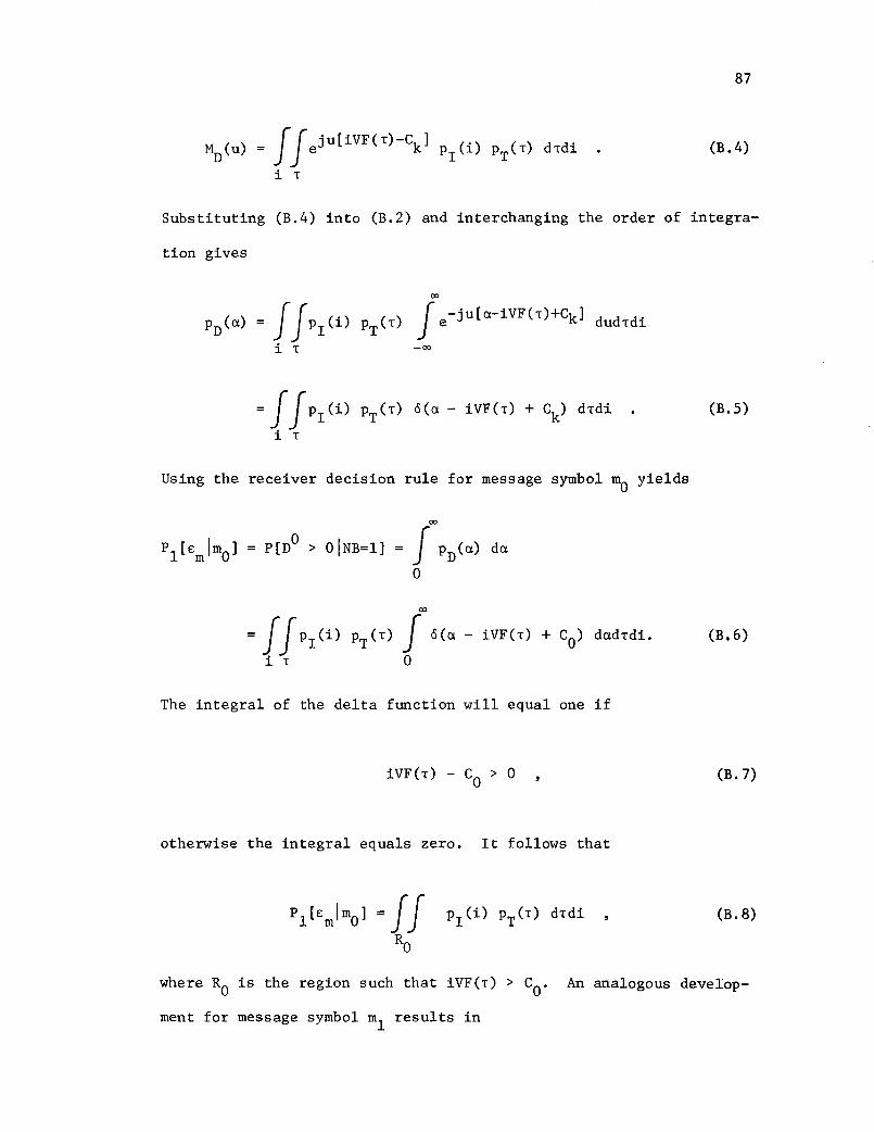
~(u) JJejU[iVF(T)-Ck ]

PI(i) PT(T) dTdi

i T

87

(B.4)

Substituting (B.4) into (B.2) and interchanging the order of integra-

tion gives

00

Pn(a) = JJPI(i) PT(T) Je-ju[a-iVF(T)+Ck] dudTdi

i T -00

=JJPI (i) PT(T) <S(a - iVF(T) + Ck) dTdi

i T

Using the receiver decision rule for message symbol mO yields

(B.5)

p[nO> OINB=l]

00

=JJPI(i) PT(T) J <S(a - iVF(T) + CO) dadTdi.

iTO

The integral of the delta function will equal one if

iVF(T) - Co > 0

otherwise the integral equals zero. It follows that

(B.6)

(B.7)

(B.8)

where RO is the region such that iVF(T) > CO. An analogous develop­

ment for message symbol ml results in

88

(B.9)

where Rl is the region such that iVF(T) < Cl • Since (B.8) and (B,9)

are equivalent to (3.35), the remainder of the error analysis is un-

changed.

APPENDIX C

COMPUTER PROGRAM: GINIMP

This appendix contains the flow chart, Fortran-IV program

listing and description for an IBM System/360 computer program

which implements the GIN model performance analysis derived in

Chapter 3. The program name, GINIMP, is an acronym for Generalized-

Impulse-Noise Implementation of Model Performance.

C.l GENERAL INFORMATION

The performance analysis for Pl[Em], is implemented for a speci­

fied data bit, signal set, ENP value, noise waveform, and weighting-

factor probability density function (p.d.f.). The user can specify

the data bit, ENP value, and one of five weighting factor density

functions through input data cards. The signal set and noise wave-

form are specified by means of input data and a function subprogram,

GRANF(x). Five typical signal sets (Unipolar, Polar, ASK, PSK, FSK)

have been incorporated into the program. Others can be added at the

user's discretion by modifying the subprogram. The input data format

and GRANF construction are explained in Section C.2.

The normalized probability of error, from (3.42), is given by

00

Pl[Em] = ~b ~ TRl(n)PN(n) dn

I . /0mln

89

(C.l)

90

Numerical techniques are used to approximate the integral solution,

Specifically, values for the p.d.f. PN(n) and the time-range function

TRI(n) are calculated for values of n between a minimum value CXN,

i.e., I i fa and a maximum value XNM. An estimate to the integral ism n

obtained by using the trapazoidal rule with upper and lower bound

calculations. An explanation of how these steps are performed is

given in Section C.2.

C.2 FLOW CHART, PROGRAM LISTING AND EXPLANATION

The flow chart of the GINIMP computer program is shown in Fig.

C-I. A program listing is presented in Fig. C-2 which is found at

the end of this Appendix. The numbers positioned beside the flow-

chart symbols indicate the level of statement numbers used in the

main program.

In the first step, two data cards are read and interpreted ac-

cording to the format and data identification given in Tables C.I

and C.2. The input ENP and SIGSET values are used to calculate the

FENP values, where

FENP (l-p )Va (C.2)

It has been shown in Section 3.3 that for selected signal sets this

is a function of the ENP value. The signal-set parameter SIGSET

determines the function to be used, cf., (3.55) and (3.56) for

specific examples. In addition, parameters used in other parts of

the program are calculated and initialized.

100

200

300

400

500

600

START

,Ir

INITIALIZEPARAMETERSSELECT FENP VALUE

,Ir

CALCULATE F1 (T)

,Ir

CALCULATE CXN, DXNPRINT HEADERS,INPUT DATA

,-CALCULATE XN(OR SL) VALUES

,r

CALCULATE TIME-RANGE DATA

,rCALCULATE!PROBABILITY~F ERROR

"PRINT OUTPUT DATA

..........

"STOP

91

Fig. C-1. GINIMP Flow Chart

92

TABLE C.l

DATA CARD 1 FORMAT AND IDENTIFICATION

SYMBOL

KBIT

TBTF

ENPM

PAD

FREQNENP

COLUMNLOCATION

1-2

3-1415-2627-3839-40

41-5253-6465-7677-80

FORMAT

12

F12.6F12.6F12.6

12

F12.6F12.6F12.6

14

EXPLANATION

KBIT*TB = Starting time of data bit beinganalyzedBit duration (in ms)Noise Waveform duration (in ms)Energy-to-Noise Parameter = EAVGTb/cr2Specifies p.d.f., Gaussian M=l, RayleighM=2, Lognormal M=3, Uniform M=4, HyperbolicM=5Parameter value associated with p.d.f.Parameter associated with noise waveformParameter associated with noise waveformNumber of ENP values used

TABLE C.2

DATA CARD 2 FORMAT AND IDENTIFICATION

SYMBOL

DF

KKKKKII

ISLMSLMXNM

SIGSET

COLUMNLOCATION

1-5

6-910-1314-17

18-2122-3334-4546-48

FORMAT

F5.2

141414

14F12.6F12.6F3.l

EXPLANATION

Specifies even step increments for SliceLevel (DF < 0), or weighting factor(DF .:. 0)Number of interpolated Fl(T) valuesNumber of calculated Fl(T) valuesNumber of Weighting-Factor values (andSlice Levels) usedSpecifies calculation of CXN (ISLM < 0)Maximum Slice-Level value to be usedMaximum Weighting-Factor value to be usedSignal Set to be analyzed, Unipolar = 1,Polar = 2, ASK = 3, PSK = 4, FSK = 5

93

The calculation of the Fl(T) data is accomplished in the second

step using (3.48), i.e.,

(KBIT+l)TB

F (T) - F(T) - 1 J f(t-T) [sl(t)-sO(t)] dt1 - l-p - (l-p)V(KBIT)TB

(C.3)

The program calculates KK+l values for the Fl array corresponding to

Fl(TJ ) for the values of TJ=(J,-l)TB/KK, where J=l,2, ... , (KK+l).

Since f(t-T)=O for t<T, it follows for the first bit that KBIT=O and

the integral in (C.3) becomes

where

Fl(T)

TB

=Ja

TB

GRANF(t)dt =J GRANF(t)dt

T

(C.4)

GRANF(t)f(t-T) [sl(t)-sO(t)]

(l-p)V (C.5)

A similar result holds for (t-T»TF. The proper limits of integration

(A to B) are determined by subroutine LIMINT which is called using the

statement CALL LIMINT(KBIT,TB,T,TF,A,B,). GRANF is provided as a func-

tion subprogram, and for the example shown in Fig. C-2 contains the

exponentially-decaying-sinusoid noise waveform, i.e.,

f(t-T) C sin[2nf (t-T)] exp[-d(t-T)]o (C.6)

Input data is used to specify f , d, and the time duration by the useo

of the mnemonics FREQ, D and TF as defined in Table C.l. The subprogram

94

calculates C such that f(t) has unit energy. The SIGSET parameter,

defined in Table C.2, is used to determine the signal set difference

[sl(t)-sO(t)]![(I-p)V]. The user must modify the f(t) and signal set

descriptions if additional forms are to be used in GRANF(t). The inte­

gration of GRANF for each TJ

is accomplished by the IBM subroutine

QATR [44]. The accuracy of each integration is specified by FPS, and

the subroutine returns an error message (IER) to indicate if the

accuracy was obtained. A printout of the header I and IER is produced.

All values of IER that indicate the accuracy FPS was not obtained are

also printed. If all integrations are within the required accuracy

the statement "ALL INTEGRATIONS WITHIN SPECIFIED ACCURACY" is printed.

The maximum value stored in the FI array, FMAX, is determined and at

the user's option (ISLM<O) used to calculate the maximum slice level

SLM.

The third step of the program, i.e., the 300 block, calculates

the beginning n-value CXN, the step size DXN for equal steps of n

values, and CC for equal slice-level step values. Printout includes

headers, input data and calculated parameters.

Values for n and the slice levels are calculated and stored in

the XN (or SL) array in the fourth step. The user specifies by the

value of DF whether the program uses equal step-size values for XN

(DF<O) or equal step-size values for SL (DF~O).

During the fifth step the time-range function TRI(n) is approxi­

mated by calculating values for the TR array. This is accomplished

by comparing each value in the FI array to each value in the SL array

and increasing the number in the TR array by one if FI(I»SL(J). A

95

linear interpolation is performed between the calculated Fl values

and each point is classified as above. The elements of the TR array

can be divided by the number of Fl points considered to yield an

approximation to TRl

(n)/Tb •

The probability of error is calculated in the last operation.

First, the TR array is modified to obtain TRl

(n)/Tb

, and the result

multiplied by the corresponding p.d.f. value obtained from the func­

tion subprogram PDF(X,M,PA). The user selects one of five p.d.f.

descriptions by selecting the proper m-parameter value as listed in

Table C.l. The PA value is a parameter used by either the lognormal

(PA>O) or the hyperbolic 3<PA<6 distributions. The numerical­

integration subroutine QTFGB is then used to calculate the approxi­

mation of Pl[Em]. The subroutine is similar to the IBM subroutine

QTFG [44], but has been modified to include upper and lower bounds

for the integral.

A printout is made from the various arrays, the most signifi­

cant of which are the cumulative probability of errors obtained

from the integration subroutine, namely POEL the lower bound, POE

the probability of error, and POEU the upper bound. The last value

in the POE array represents Pl[Em], and two checks for accuracy can

be performed. First, the values of POE should converge to the last

value. If this does not happen, the user should increase the maximum

value of n, XNM, and repeat the computation until convergence is

obtained. Second, the lower and upper bounds can be compared to the

POE value to determine if a sufficient number of XN values (II) were

used.

96

DIMENSION TRCSOO),SLC500),ANP(SOO),AUX(SOO),F1CSOO)DOUBLE PRECISION CXN,DXN,XNCSOO),POECSOO),POELCSOO)DOUBLE PRECISION POEU(SOO)EXTERNAL GRANFCOMMON T,TF,FREQ,D,ISIGREADCS,101)KBIT,TB,TF,ENP,M,PA,D,FREQ,NENP

101 FORMATCI2,3F12.6,12,3F12.6,I4)READCS,102)DF,KKK,KK,II,ISLM,SLM,XNM,SIGSET

102 FORMATCFS.2,414,2F12.6,F3.1)IRE=OI II =SOOISIG=SIGSETDO 60S IENP=1,NENPIFCIENP.EQ.1) GO TO 107ENP=10.*ENP

107 CONTINUEGO TOC103,104,10S,103,103),ISIG

103 FENP=SQRTCENP/2.)GO TO 106

104 FENP=SQRTCENP)GO TO 106

lOS FENP=SQRTCENP/4.)106 CONT INUE

IFCIENP.GE.2) GO TO 301C***********************************************************C SETS UP CONDITIONS, DETERMINES LIMITS, CALCULATES FCT)C FOR EACH VALUE OF T SPECIFIED, AND STORES RESULTS INC THE F1 ARRAYC

FMAX=O.DTT=TB/C1000.*KK*KKK)KK 1=KK+1KKK 1=KKK+1WRIT EC6 , 200 )

200 FORMATC '0',4X,' I',4X,'IER',I,'**********************',1'***************************************************' )

DO 204 I=1,KK1T=CI-1)*TB/KKCALL LIMINTCKBIT,TB,T,TF,A,B)FPS=1.0E-7A=A*.OOlB=B*.OOlCALL QATRCA,B,FPS,III,GRANF,Y,IER,AUX)F 1 CI ) =YIF(IER) 201,203,201

201 CONTINUEIRE = IRE+1WRITEC6,202)I,IER

Fig. C-2. GINIMP Program Listing

202 FORMAT(2X,214)203 CON TINUE

YABS=ABS(Y)IF(YABS.LT.FMAX)GO TO 204FMAX=YABS

204 CONTINUEIF (IRE) 508,506,508

506 WRITEI6,507)507 FORMAT(ZX,'ALL INTEGRATIONS WITHIN SPECIFIED ACCURACY')508 CONT INUE

IF ( ISLM) Z05, 205, 301205 SLM=FMAX+.000001c***********************************************************C CALCULATES PARAMETERS BASED ON INPUT DATA,C HEADER AND DATA OUTPUTC301 CXN=FENP/SLM

o XN= (XNM-C XN ) / ( I 1-1 )TR(l)=O.Sll 1 )=0.XN ( II ) =10**4XNl1 )=CXNSL (II )=FENP/CXNCC=SLM/(II-1)WRITE(6,30Z) SIGSET

302 FORMAT('l',ZOX, 'PERFORMANCE ANALYSIS FOR GIN MODEL "l'AND SIGSET=',F3.1,/,ZX,'***************************',1'***************************************************',l'*****',/,ZX,'THE INPUT PARAMETERS ARE',/)

WRITEI6,304)304 FORMAT(6X,'KBIT',8X,'TB',10X,'TF',9X,'ENP',9X,'M',9X,

1 ' PA ' , lOX, ' D' , lOX, ' FRE Q' )WRITE(6,305) KBIT,TB,TF,ENP,M,PA,D,FREQ

305 FORMAT(7X,IZ,5X,3F12.8,ZX,IZ,lX,3F1Z.4,/)~JRITEI6,306)

306 FORMAT (9X, 'OF', 8X, 'KKK', lX,' KK' ,ZX,' I I' ,4X, 'CXN' ,9X,1 'D XN ' ,9X, ' SU·'I' )

WRITE(6,307)DF,KKK,KK,II,CXN,DXN,SLM307 FORMAT(6X,F1Z.8,314,3F1Z.8)

WRITE(6,309)309 FORMAT(ZX,lZ(/),ZX,'NOISE WAVEFORM USED****',

l'EXPONENTIALLY DECAYING SINUSOID')c***********************************************************C CALCULATES EVEN SL OR EVEN XNC

IF(DF)403,401,401401 DO 402 J=2,II

TR(J)=O.

Fig. C-2 (Continued). GINIMP Program Listing

97

98

S L( J )= ( J-1 )*C C402 XN(II+1-J)=FENP/SL(J)

GO TO 405403 DO 404 1=2,11

TR(I)=O.XN I I) =XN ( 1-1 I+DXN

404 SUII+1-1)=FENP/XN(I)405 CONTINUEc***********************************************************C INTERPOLATES AND CLASSIFIES THE F(T) VALUESC

DO 505 1=2,KK1IF(I.LT.KK1) GO TO 501JJK=KKKIGO TO 502

501 JJK=KKK502 DO 504 J=l,JJK

TT =(J -1 ) *0TTF2=ABS ( (F 1 ( I )-F 1 ( 1-1 ) ) * ( (J -1 ) / KKK) +F 1 ( 1-1 ) )DO 504 L=l,III F( F2 • GE• SL( L» GO TO 503GO TO 504

503 TRIL)=TR(L)+l504 CONTINUE505 CON TIN UEc***********************************************************C CALCULATES THE PROBABILITY OF ERRORC

WRITE(6,60l>601 FORMAT('1',80X,'CUMULATIVE PROBABILITY OF ERROR',1,5X,

1 I I I , lOX, I XNI , 14 X, I SL I , 14X, IT R' , 13X , ' AN P , , 12 X, , LOW ER ' ,111X,'AVERAGE',9X,'UPPER',/,2X,'*********************',1'***************************************************',1'**************************************************')

DO 604 1=1, I ITRII)=TR(I)/(KK*KKK+1)I NE W= I 1+1- IYPDF=PDF (XN (INEW) ,M,PA)ANP(INEW)=TR(II*YPDF

604 CONTINUECALL QTFGB(XN,ANP,POE,POEL,POEU,IIIWRITE(6,603) (I ,XN( I ),SL( I 1+1-1 ),TR( 11+1-1) ,ANP( I I,

1POE L ( I ) , POE ( I I , PO EU( I ) , 1=1 , I I )603 FORMAT(2X,14,7F16.9)605 CONTINUE

STOPEND

Fig. C-2 (Continued). GINIMP Program Listing

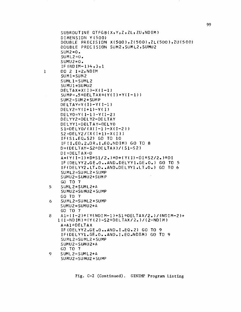
SUBROUTINE QTFGBCX,Y,Z,ZL,ZU,NDIM)DIMENSION Y(500)DOUBLE PRECISION X(500),ZC500),ZLC500),ZUC500)DOUBLE PRECISION SUMZ,SUMLZ,SUMU2SUMZ=O.SU MLZ =0.SUMU2=O.IF CNDIM-l)4,3,1

1 DO 2 I=2,NDIMSUM1=SUM2SUML l=SUMLZSUMU1=SUMU2DELTAX=XCI)-XCI-l)SUMP=.5*DELTAX*(YCI)+YCI-l»SUM2 =SUMZ+ SUM PDELTAY=YCI)-YCI-l)DELY2=YC I+l)-Y( I)DELYO=YCI-l)-YCI-2)DELYY2=DELY2-DELTAYDELYY1=DELTAY-DELYOSl=DELYO/(XCI-l )-XCI-2»S2=DELY2/(XC I+l}-X( I»IFCSl.EQ.SZ) GO TO 10IFCI.EQ.2.0R.I.EQ.NDIM) GO TO 8D=CDELTAY-S2*DElTAX)/(SI-S2)DI=DELTAX-DA=CY(I-l)+D*Sl/Z.)*D+(YCI)-DI*SZ/2.)*DIIFCDELYY2.GE.0 •• AND.DELYYl.GE.O.) GO TO 5IFCDElYY2.lT.O •• AND.DElYYl.lT.0.) GO TO 6SUML2=SUMLZ+SUMPsur~U2=SUMUZ+SUM PGO TO 7

5 SUMLZ=SUMlZ+ASU MU2=SUMUZ +SUMPGO TO 7

6 SUML2=SUMl2+SUMPSUMU2=SUMU2+AGO TO 7

8 Al=CI-2)*CYCNDIM-l)+SI*DELTAX/Z.)/CNDIM-2)+lCI-NDIM)*CYC2)-S2*DELTAX/2.)/C2-NDIM)

A=A 1to' 0 ELTAXIFCDELYY2.GE.0 •• AND.I.EQ.Z) GO TO 9IFCDELYYl.GE.O •• AND.I.EQ.NDIM) GO TO 9SUML2=SUML2+SUMPSUMU2=SUMUZ+AGO TO 7

9 SUML2=SUML2+ASUMU2=SUMUZ+SUMP

Fig. C-2 (Continued). GINIMP Program Listing

99

100

GO TO 710 SUML2=SUML2+SUMP

SU MU 2 =SU MU2 + SUMP7 ZLl 1-1 )=SUMl1

ZU I 1-1 ) = SUM U 12 Z ( 1- 1 ) = SU M13 ZINDIM)=SUM2

Z Ll NDIM ) = SUM L 2ZU I NDIM ) =SU MU2

4 RETURNEND

c***********************************************************c

SUBROUTINE lIMINT(KBIT,TB,T,TF,A,B)J=TF/TBIFIKBIT.GT.O•• AND.KBIT.lT.J) GO TO 50IF(KBIT.EQ.O •• AND.J.EQ.O.) GO TO 53IFIKBIT.GT.O•• AND.J.EQ.KBIT) GO TO 55IFIKBIT.EQ.(J+1.» GO TO 51IF(KBIT.EQ.O •• AND.J.GT.O.) GO TO 57GO TO 58

50 A=KB IT*TBB= I KB IT+ 1.) ::<TBGO TO 58

51 IFI(T+TF).lE.KBIT*TB) GO TO 5256 A=KB IT*TB

B=T+TFGO TO 58

52 A=O.B=O.GO TO 58

53 1F I (T + TF ) • l E • TB) GO TO 5457 A=T

B=TBGO TO 58

54 A=TB=T+TFGO TO 58

55 IF«T+TF).lE.«KBIT+1.)*TB» GO TO 56GO TO 50

58 RETURNEND

Fig. C-2 (Continued). GINIMP Program List~ng

101

FUNCTION GRANF(X)COMMON T,TF,FREQ,O,ISIGF=FREQTFF=TF*.OOlPI=3.14159265358979A=1./(PI*F)*SQRT«O*(O**2+4.*(PI*F)**2))/(1-EXP(-

12.*D*TFF)) )GRANF=A*SIN(2.*PI*F*(X-T*.OOl))*EXP(-D*(X-T*.001) )GO TO(1,1,2,2,3),ISIG

1 RETURN2 GRANF=GRANF*SIN(2000.*PI*X)

RETURN3 GRANF=GRANF*(SIN(2000.*PI*X)-SIN(4000.*PI*X))

RETURNEND

C***********************************************************C

FUNCTION POF(X,M,PA)PI=3.14159265358979GO TO(1,2,3,4,5),M

1 PDF=(1/SQRT(2.*PI))*EXP(-X**2/2.)RETURN

2 PDF=ABS(X)*EXP(-X**2)RETURN

3 P01=1/(SQRT(8.*PI)*PA*ABS(X))PD2=EXP(-(AlOG(ABS(X))+PA**2)**2/(2.*PA**2) )PDF=PD1*P02RETURN

4 Z=ABS(X)IF(Z-SQRT(3.))41,41,42

41 PDF=1/SQRT(12.)RETURN

42 PDF=ORETURN

5 PD3=(PA-l)*«PA-2.)*(PA-3.))**«PA-l)/2.)PD4=(SQRT( (PA-2.)*(PA-3.))+SQRT(2.)*ABS(X))**PAPDF=1/SQRT(2.)*PD3/PD4RETURNEND

Fig. C-2 (Continued). GINIMP Program Listing

APPENDIX D

COMPUTER PROGRAM: LIMITER

The Fortran-IV computer program LIMITER implements the perfor-

mance results of Section 5.2. The program name is a mnemonic to

emphasize the association with the generalized limiter of Fig. 5.2.

A succinct explanation of this program is presented by the use of a

flow chart and program listing.

D.l GENERAL INFORMATION

The program implements (5.12) to calculate P1[£m1mj] for a

given data bit, signal set, ENP value, noise waveform, limiter

parameters, and weighting factor p.d.f. The use of either positive

or negative values for the weighting factor must also be controlled.

These parameters are specified by input data and function subprograms.

Four typical signal sets (Unipolar, Polar, ASK and PSK) and the five

weighting-factor p.d.f.s of Table 3.1 have been incorporated into the

program. Numerical techniques are used to approximate the integral

solutions. The minimum weighting-factor value can be specified or

calculated in the program by an iteration process. An explanation

of the program operation is given in Section D.2.

102

103

D.2 FLOW CHART, PROGRAM LISTING AND EXPLANATION

The LIMITER program flow chart is shown in Fig. D-l. A program

listing is presented in Fig. D-2, which is located at the end of this

Appendix. The first symbol represents the operations performed by

statement numbers 0 through 299. Five data cards are read by the

format and data identification given in Tables D.l through D.S. Two

arrays are calculated based on the function subprogram specification

of the signal set and noise waveform. The ENP value is selected from

the ENPA array and the program is initialized for positive or negative

weighting-factor calculations. The calculation of cO/(av) is made

according to the signal set selected. Headers and data are printed

and parameters are initialized for the weighting factor iteration

process.

TABLE D.l

DATA CARD 1 FORMAT AND IDENrIFICATION

,

COLUMNSYMBOL LOCATION FORMAT EXPLANATION

ENPA(l) 2-13 F12.l0 ENPA is a one-dimensional array withENPA(2) 14-25 FJ,2.10 three elements containing the ENPENPA(3) 26-37 F12.l0 Values

The second step in the flow chart corresponds to operations per-

formed by statements with numbers 300 through 899. Normally, the

iteration process for the minimum positive (or maximum negative)

weighting factor will be utilized (by specifying ISCH = 1). The

0-200

300-800

900

( START

,r

PARAMETERSINITIALIZED

--,Ir

DETERMINE N i 'ronFj(n,T), TR(n)

CALCULATE TR(n) *PN(n) for each nVALUE

DETERMINEPROBABILITY OFERROR, PI [Em Iroi]

PRINTPROBABILITY

--..oF ERROR

"STOP

104

Fig. D-l. LIMITER Flow Chart

105

time-range function is calculated for a weighting-factor value of

CXO/2. Successive approximation steps in the weighting-factor value

are made in the iteration attempt to locate the largest value that

gives a zero value for the time range. After this operation is com-

plete, the array of weighting-factor values is finalized. The non-

linear operation {Nf(t_T)}oOO is performed in the series of steps

through the 500-level statement numbers. These results are mul-

tiplied by the signal-set array data and integrated in the 600-level

statements. An approximation to the time-range function is made in

the 700-level statements by classifying and interpolating the integral

results that exceed cO/(aV).

TABLE D.2

DATA CARD 2 "FORMAT AND IDENTIFICATION

COLUMNSYMBOL LOCATION FORMAT EXPLANATION

SIGSET 3-13 FlO.4 Signal Set to be analyzed, Unipolar = 1,Polar = 2, ASK = 3, PSK = 4

Fl 14-23 FlO.4 Frequency of sl(t) for ASK and PSKFa 24-33 F10.4 Not used, intended for frequency of

34-37 14sO(t) for FSK.

KBIT KBIT*TB = Starting time of data bitbeing analyzed

MPDF 38-41 14 Specifies p.d.f., Gaussian = 1,Rayleigh = 2, Lognormal = 3, Uniform =4, and Hyperbolic = 5

PA 42-51 F10.8 Parameter value associated with p.d.LTB 52-61 F10.8 Bit duration (in sec)

Multiplication of the time-range data by the corresponding p.d.f.

values is accomplished by the 900-1eve1 program statements. Headers

106

and output data are printed. An estimate of the error probability

is calculated in the last step. The results are presented graphically

with the final value in the graph representing the estimate. Checks

for convergence of the integral and correct weighting-factor step size

should be made.

TABLE D.3

DATA CARD 3 FORMAT AND IDENTIFICATION

SYMBOL

NIPF

NTL

NTLTNXN

CONN

CONP

XNMPXNMN

COLUMNLOCATION

3-6

7-10

11-1415-18

19-28

29-38

39-4849-58

FORMAT

14

14

1414

FlO.3

FlO.3

FlO.4FlO.4

EXPLANATION

Number of interpolated points betweeneach time-shift pointNumber of sample points used in bit timeTbNumber of NTL samples per time shiftNumber of Weighting-Factor values usedbetween minimum and maximum valuesDefines LIMITER operation,

Sn = ICONN anDefines LIMITER operation,

Sp = ICONP apMaximum positive Weighting-Factor valueMinimum negative Weighting-Factor value

TABLE D.4

DATA CARD 4 FORMAT AND IDENTIFICATION

107

COLUMNSYMBOL LOCATION FORMAT EXPLANATION

CXNP (1) 1-10 F10.7 CXNP is a one-dimensional area with threeCXNN(l) 11-20 F10.7 elements containing the minimum positiveCXNP(2) 21-30 F10.7 Weighting-Factor v~lues for each of theCXNN(2) 31-40 F10.7 three ENP values. CXNN is a similar arrayCXNP(3) 41-50 F10.7 for the maximum negative Weighting-FactorCXNN(3) 51-60 F10.7 values.

TABLE D.5

DATA CARD 5 FORMAT AND IDENTIFICATION

COLUMNSYMBOL LOCATION FORMAT EXPLANATION

MJ 3-6 14 Message symbol to be analy~ed mO=O,ml=lICXN 7-10 14 Specifies sign of Weighting-Factor values

Positive = 1, Negative = 2ISCH 11-14 14 Specifies use CXNP or CXNN (ISCH=O) o:r

iteration routine to calculate value(ISCH=l)

CXO 15-26 F12.6 Maximum value of iteration step

108

o I I'·', Er\j S 10 r,! X ~< (600 ) , T I HE ( f, 0 0 ) , X ~~ F ( 1200 ) , SX ~I F ( 6 (0) ,1 SA ( 6 00 ) , Y Y ( 10 1 ) , Z ( 600) , ZZ ( 1 0 0 ) , A i'J S ( J. 00 ) , J: 1\1 P A ( 3 ) , CXN i'~ ( 3 ) ,1 FA ( 1200) , CXI'! P ( 3)

COf-!i-·'t()i·J F1, FOPI=3.14159265358979RE'w (5 , 6) ( E~.J PA ( I ) , I =1 , 3 )

6 FORMAT(1X,3F12.10)READ(5,1)SIGSET,F1,FO,KBIT,NPOF,PA,TR

1 FORMAT(2X,3F10.4,2I4,2F10.B)REA 0 ( 5 , 2 ) i'~ I PF , ,,! T L , i'JT L T , f\I Xi'l , CON N , CO J\! P , Xf\j HP , X 1\1i"j\1

2 FORMAT(2X,4I4,4F10.3)REAO(5,5) (CXf'JP( I),CXf\!f'I(1),1=1,3)

5 FOR~AT(6F10.7)

READ(5,4)MJ,1CXN,ISCH,CXO4 FORMAT(ZX,314,F12.6)

\1 RI T E ( 6 ,3 ) S Il; SET, F 1 , F0 , KBIT, Iv) PDF, P A , T B , NIP F , 1\1 T L , 1\: T LT ,u: X r\) , Cor,j[\] , co N P , XNlvj P, XN Ivll\]

3 FOR 1/1 AT ( , 1 ' , 2 X, , ,;, ':' ,;,: ,;, *,;, ,;, ':' ,;, ,;, ,;, ,;, ,;, ,;, ':' ':' ,;, ':' ,;, ,;, ,;, ,;, ,;, ,;, ,;, ,;, ,;, ,;, ,;, ,;, ':' ':' ,;, ,;, ,;, ,;, ,;, , ,

1'PERFORMANCE ANALYSIS USING LIMITER',/,3X,'SI~SFT',

1 Lt X , , F l' , 8 X, 'F 0 ' ,8 X, , K BIT' ,1 X, , HP OF ' , 1 X, 'P A ' ,9 X, , T R ' ,1 / , 2 X , 3 F 10 • 4 , 2 I 4 , 2 X , F 10 • 8 , 1 X , F 1 0 • 8 , / / , 2 X, '~I I P F' , 1. X ,1 'In L ' , 1 X , '~,I T L T ' , 1 X , , [\1 XN ' , 4X , , CON [\1 ' , 6 X , , Cm·1 P , , 6 X ,1 ' XI\! 1,1 pi, 6 X , 'X, I i\'1r,1 , , / , 2 X , 4 I 4, 4 F 10 • 3 )

1SIG=SIGSEToT L=T B / (f\JT L- 1 )

C CALCUATE SA M.10 FA ARRI-\YSoCJ 1 0 1 I = 1 ,I'JT LTL =(1-1) ';'rn LT FIE ( I ) =T LSA(I)=S(TL,ISIG)TTL=(KB1T-1)*TB+TLTTTL=TTL+TBFA( I )=F (TTLl

1 0 1 F A ( f\; T L + I ) =F ( T TTL )C SELECT ENP, CXN, XNM AND FENPC PRli'!T HEADER Af'JD INPUT DATAC Ii'! I T I 1\ LIZ E F LH~ CXI\J ITERA T I 01\1

DO 910 IEf,IP=1,3IF ( I CX ~.; -1 ) 202 ,202,203

202 CXN=CXNP(IENP)Xi\'i·· =XI·I j·i PGO TO 204

203 CXr-i=CX~..Jf-H1ENI-')Xr< I'! =X/,jhf'i

204 cmn If-.JUEE;\! P=E r-W /.\ ( IE N 1-' )GO TO (210,211,212,213,214),1SIG

Fig. D-2. LIMITER Program Listing

109

210 FENP=SQRTIENP/2.)GO TO 215

~11 FENP=SQRTIENP)GO TO 215

212 FENP=SQRTIENP/4.)GO TO 215

213 FENP=SQRTIENP/2.)GO TO 215

214 FENP=SC.;lRTIENP/2.)215 CONTINUE

WRI TEl 6 , 2 9 2 ) Ef\J P , MJ , I CXN, CXf\j

292 FOR r'l ATI I 1 ' , 'T HE F0 LLOW I NG ANALYSIS I S FOR Ef\1 P=, , F12 •8 ,15 X, 'M J = , , 12, 5X, , I CXN =' , 12, 5X, , CXN=, , F12.6, I )

CXS =C XOI CYXN=OISTEP=OI XF X=I SCH

CITERAT 10 N FOR CX NIP ART 1)H68 CXS=CXS/2.

ISTEP=ISTEP+lWRITEI6,872)ISTEP,ICYXN,CXN

872 FORMATI2X,'THE',I3,2X,'STEP YIELDS ICYXN=',I5,~X,'AND',

l' CXN=',FI2.6)IFIISTEP.EQ.50) GO TO 910IFIISTEP.EQ.2.AND.ICYXN.EC.0) GO TO 910IF I ICYXN )866,866,867

H66 Cxr~ =CXf\J +C XSGO TO 860

867 CXN=CXN-CXS860 DXN=IXNM-CXN)/INXN-9)C CALCUATE XN VALUES

DO 201 IXN=I,NXNICYXN=OI F (l XN• GE• 1 • AN D. I XN• LT. 11 ) GO TO 250XXN= I I XN-9 )*DXN +CXNGO TO 251

250 XXN=(IXN-l)*(DXN/9.)+CXN251 XN I I XN ) =XXNC MULTIPLY EACH FA BY XN

DO 301 I=I,NTLXNF I I ) =XXN *FA ( I )INTL=NTL+I

301 XNF(INTLl=XXN;'<FA(INTllC TIME SHIFT XN*FA

NT=INTL/NTLT)+1DO 401 J=I,NTIT=IJ-l)*NTLT

C THE INDEX IT CORRESPONDS TO THE TIME SHIFT T

Fig. D-2 (Continued). LIMITER Program Listing

DO 405 L=l,NTL405 SXNFIL)=XNFINTL-IT+L)C CLIP SHIFTED XN*FA

DO 509 L=l,NTLTL=IKBIT-1)*TB+(L-1)*DTLIFIMJ-1)507,508,508

507 GO TO 15071,5072,5073,5074,5075),ISIG5071 DUML=O.

DUMU=SQRTI2.*ENP/(TB**2»GO TO 510

5072 DUML=O.DUMU=SQRT(4.*ENP/ITB**2»GO TO 510

5073 DUML=-SQRT(4.*ENP/(TB**2»DUMU=SQRT(4~*ENP/(TB**2»

GO TO 5105074 DUML=-SQRT(2.*ENP/ITB**2) )*(1.-SIN(2.*PI*F1*TL»

DUMU=SQRT(2.*ENP/(TB**2»*11.+SIN(2.*PI*F1*TL) )GO TO 510

5075 DUML=O.DUMU=O.GO TO 510

508 GO TO (5081,5082,5083,5084,5085),ISIG5081 DUML=-SQRT(2.*ENP/ITB**2»

DUMU=O.GO TO 510

5082 DUML=-SQRT(4.*ENP/(TB**2»DUMU=O.GO TO 510

5083 DUML=-SQRT(4.*ENP/(TB**2»*(1.+SIN(2.*PI*F1*TL»DUMU=SQRTI4.*ENP/(TB**2»*(1.-SINI2.*PI*F1*TL»GO TO 510

5084 DUML=-SQRTI2.*ENP/(TB~~~~2))*11.+SIN(2.*PI*F1*TL»DUMU=SQRT(2.*ENP/(TB**2»*11.-SIN(2.*PI*F1*TL) )GO TO 510

5085 DUML =0.DUMU=O.

510 CONTINUEIFISXNF(L).GE.DUML.AND.SXNF(L).LE.DUMU) GO TO 517IFISXNF(L).GT.DUMU.AND.MJ.EQ.O) GO TO 513IF(SXNF(L).GT.DUMU.AND.MJ.EQ.1) GO TO 514IF(SXNFIL).LT.DUML.AND.MJ.EQ.O) GO TO 515IFISXNF(L).LT.DUML.AND.MJ.EQ.1) GO TO 516

513 GO TO (5131,5132,5133,5134,5135),ISIG5131 SXNFIL)=SQRTI2.*CONP*ENP/ITB**2»

GO TO 5175132 SXNF(L)=SQRTIENP/(TB**2) )*(SQRT(CONP)+1.)

GO TO 517

Fig. D-2 (Continued). LIMITER Program Listing

110

5133 SXNF(L)=SQRT(4.*CONP*ENP/(TB**2»GO TO 517

5134 SXNF(L)=SQRT(2.*ENP/(TB**2»*(SQRT(CONP)+1 SIN (2 .;'< P I >:'F 1 ':<T L) )

GO TO 5175135 SXNF(L)=O.

GO TO 517514 GO TO (5141,5142,5143,5144 t 5145),ISIG5141 SXNF(L)=SQRT(2.*ENP/(TB**2»*(SQRT(CONP)-1.)

GO TO 5175142 SXNF(L)=SQRT(ENP/(TB**2»*(SQRT(CONP)-1.)

GO TO 5175143 SXNF(L)=SQRT(4.*ENP/(TB**2»*(SQRT(CONP)­

1 SIN (2 •* P I :::'F 1*TL) )

GO TO 5175144 SXNF(L)=SQRT(2.*ENP/(TB**2»*(SQRT(CONP)­

1S IN (2. :::'PI *F1~"TL »GO TO 51 7

5 145 SXN F ( L ) =0 •GO TO 51 7

515 GO TO (5151,5152,5153,5154,5155),ISIG5151 SXNF(L)=-SQRT(2.*CONN*ENP/(TB**2»

GO TO 5175152 SXNF(L)=SQRT(ENP/(TB**2»*(-SQRT(CONN)+1.)

GO TO 5175153 SXNF(L)=-SQRT(4.*CONN*ENP/(TB**2»

GO TO 5175154 SXNF(L)=SQRT(2.*ENP/(TB**2»*(-SQRT(CONN)+

1S IN (2.*PI*Fl':<TL»GO TO 517"

5 155 S XN F ( L ) =0 •GO TO 51 7

516 GO TO (5161,5162,5163,5164,5165),ISIG5161 SXNF(L)=SQRT(2.*ENP/(TB**2»*(-SQRT(CONN)-1.)

GO TO 5175162 SXNF(L)=SQRT(ENP/(TB**2»*(-SQRT(CONN)-1.)

GO TO 5175163 SXNF(L)=SQRT(4.*ENP/(TB**2»*(-SQRT(CONN)-

1SIN(2.*PI*F1*TL»GO TO 51 7

5164 SXNF(L)=SQRT(2.*ENP/(TB**2»*(-SQRT(CONN)­1 SIN (2 •*P I*F 1;'<T L) )

GO TO 5175165 SXNF(L)=O.517 CONT INUE509 CONTINUEC SXNF NOW REPRESENTS SHIFTED AND CLIPPED XNFC

Fig. D-2 (Continued). LIMITER Program Listing

111

112

C MULTIPLY CLIPPED XN*FA BY SAC INTEGRATE TO OBTAIN FJ(N,TI AND STORE IN YY ARRAY

DO 601 ~1=1,NTL

601 SXNF(M)=SXNF(M)*SA(M)CALL QTFGlTHIE,SXNF,l,NTLIIF(MJ)602,602,603

602 YY(JI=Z(NTL)GO TO 401

603 YY(J)=-Z(NTLI40 1 CON TIN UEC INTERPOLATE AND CLASSIFY FJ(N,T) VALUES TO OBTAINC TIME RANGE DATA

DO 701 IC=2,J\JTIF(YY(IC-ll.LT.FENP.AND.YY(IC).LT.FENP) GO TO 701IF ( IC-N T )704 , 7 05 , 705

705 NIP=NIPFC NIPF IS THE NUMBER OF INTERPOLATED POINTS FIXED

GO TO 706704 NIP=NIPF-1706 DO 703 ICC=1,NI PC NIP IS NUMBER INTERPOLATED POINTS

YDUM=( (YY( IC)-YY(IC-l1 )~:«ICC-l1 )/(NIPF-1)+YY(IC-l)IF (YDUM-FENPI703,707,707

707 ICYXN=ICYXN+l703 CONTINUE70 1 CON TIN UEC IT ERATION FOR CXN (PART 2 I

YK= I CYXNIF(IXFX.EQ.O)GO TO 970IF(ICYXN.GT.0.AND.ICYXN.LE.4)GO TO 871GO TO 868

871 IXFX=OC MULTIPLY TIME RANGE DATA BY PDF VALUESC PRINT HEADER AND OUTPUT DATA9 70 AN S ( I XN ) =(YK/ ( INIP F- 1 )::q NT- 1 )+1 ) I* PDF (XN( I XN) , ~-1 PDF, PAI

IF(IXN-l)973,973,974973 WRITE16,9751975 FORMAT (3X, '1XN' ,l5X, 'YK' ,l8X, 'ANS')974 WRITE(6,991) IXN,YK,ANS(IXNI991 FORMAT(2X,I4,10X,F12.6,10X,F12.61201 CONTINUEC CALCUATE PROBABILITY OF ERROR900 CALL QTFG(XN,ANS,ll,NXNI

CALL GRAPH1(XN,ZZ,NXN,2)WRITE(6,499) IYY(JI,J=1,NT)

499 FORMATI2X,10F11.6)910 CONTINUE

STOPEND

Fig. D-2 (Continued). LIMITER Program Listing

113

FUNCTION S(TL,ISIG)COM MOf\J F 1 , F 0PI=3.14159265358979GO TOll,2,3,4,5),ISIG

1 S =1 •RETURN

2 S=1.RETURN

3 S=SIN(2.*PI*F1*TL)RETURN

4 S=SIN(2.*PI*F1*TL)RETURN

5 S=SIN(Z.*PI*F1*TL)-SIN(2.*PI*FO*Tl)RETURNEND

c***********************************************************C

FUNCTION F(X)IF(X)9,8,8

8 CONTINUETFF=.004IF (X-TFF )11,11,9

11 0=500.C FREQ=G

G=1000.PI=3.14159265358979A=I./(PI*G)*SORT«0*10**2+4.*(PI*G)**Z»/(1-EXP(-Z*0*TFF»)F=A*SIN(Z.*PI*G*X)*EXP(-O*X)GO TO 10

9 F=O.10 RETURN

END

Fig. D-2 (Continued). LIMITER.Program Listing

LIST OF REFERENCES

1. J. H. Fennick, "Amplitude Distributions of Telephone Channel Noiseand a Model for Impulse Noise," Bell System Technical Journal, vol.48, pp. 3243-3263, December 1969.

2. M. Kurland and D. A. Molony, "Observations on the Effects of PulseNoise in Digital Data Transmission Systems," !~EE Transactions onCommunication Technology, vol. COM-15, pp. 552-555, .August 1967.

3. P. Mertz, "Model of Impulsive Noise for Data Transmission," IREConvention Record, Part 5 - Communication Systems, pp. 247-259,March 1960.

4. P. Mertz, "Model of Error Burst Structure in Data Transmission,"Proceedings of the National Electronics Conference, vol. 16, pp.232-240, October 1960.

5. P. Mertz, "Appraisal of Error Performance in Data Transmission,"DDC Report No. AD 606 658, July 1962.

6. B. Shepelavey, "Non-Gaussian Atmospheric Noise ip Binary-Data,Phase-Coherent Communication Systems," IEEE Transactions onCommunication Systems, vol. CS-ll, pp. 280-284, September 1963.

7. A. J. Rainal, "Statistical Properties of Noise Pulses," The JohnHopkins Univ~rsity Carlyle Barton Laboratory, Technical ReportNo. AF-l09, June 1964.

8. K. F. Tuncer, "Non-Gaussian Noise," NASA Research Grant 19-003­003, Progress Report, May 1970.

9. J. C. Lindenlaub and K. A. Chen, "Performance of Matched FilterReceivers in Non-Gaussian Noise Environments," IEEE Transactionson Communication Technology, vol. COM-13, pp. 545-547, December1965.

,10. R. E. Ziemer, "Character Error Probabilities for M-ary Signalingin Impulsive Noise Environments," IEEE Transactions on Communica­tion Technology, vol. COM-15, pp. 32-44, February 1967.

11. R. C. Houts and J. D. Moore, "Study of Correlation Receiver Per­formances in the Presence of Impulse Noise," Technical Report No.129-102, Communication Systems Group, Bureau of Engineering Re­search, University of Alabama, February 1971.

114

115

12. P. A. Bello and R. Esposito, "A New Method for CalculatingProbabilities of Errors Due to Impulsive Noise," IEEE Trans­action on Communication Technology, vol. COM-17, pp. 368-379,June 1969.

13. P. A. Bello and R. Esposito, "Error Probabilities Due to Impul­sive Noise in Linear and Hard-Limited DPSK Systems," IEEE Trans­actions on Communication Technology, vol. COM-19, pp. 14-20,February 1971.

14. L. R. Halsted, "On Binary Data Transmission Error Rates Due toCombinations of Gaussian and Impulse Noise," IEEE Transactionson Communication Systems, vol. CS-ll, pp. 428-435, December 1963.

15. J. H. Halton and A. D. Spaulding, "Error Rates in DifferentiallyCoherent Phase Systems in Non-Gaussian Noise," IEEE Transactionson Communication Technology, vol. COM-14, pp. 594-601, October1966.

16. G. D. Arndt and F. J. Loch, "Correlation Detection of ImpulseNoise for PM Threshold Extension," Proceedings of IEEE, vol. 58,pp. 1141-1143, July 1970.

17. R. W. Chang, "A New Digital Frequency Detection Scheme," IEEETransactions on Communication Technology, vol. COM-18, pp:-305-3l2,August 1970.

18. A. M. Conda, "The Effect of Atmospheric Noise on the Probabilityof Error for an NCFSK System," IEEE Transactions on CommunicationTechnology, vol. COM-13, pp. 280-284, September 1965.

19. R. Esposito and J. F. Roche, "Characterization of Man-Made Noiseand Prediction of Error Rate in VHF Digital Systems," 1970 Inter­national Conference on Communications, vol. 1, pp. 10-(1-5), June1970.

20. J. H. Fennick, "A New Method for the Evaluation of Data SystemsSubject to Large Noise Pulses," IEEE International ConventionRecord, Part I, Communications 1, Wire and Data Communications,pp. 106-110, March 1965.

21. R. E. Ziemer, "Error Probabilities Due to Additive Combinationsof Gaussian and Impulsive Noise," IEEE Transactions on Communi­cation Technology, vol. COM-15, pp. 471-474, June 1967.

22. P. A. Bello, "Error Probabilities Due to Atmospheric Noise andFlat Fading in HF Ionospheric Communication Systems," IEEE Trans­actions on Communication Technology, vol. COM-13, pp. 266-279,September 1965.

/.'"

116

23. A. B. Bodonyi, "Effects of Impulse Noise on Digital Data Trans­mission," IRE Transactions on Communication Systems, vol. CS-9,pp. 355-361, December 1961.

24. J. S. Engel, "Digital Transmission in the Presence of ImpulsiveNoise," Bell System Technical Journal, vol. 44, pp. 1699-1743,October 1965.

25. J. B. Millard and L. Kurz, "Adaptive Threshold Detection ofM-ary Signals in Statistically Undefined Noise," IEEE Transac­tions on Communication Technology, vol. COM-14, pp. 601-610,October 1966.

26. w. L. Black, "An Impulse Noise Canceller," IEEE Transactions onCommunication Systems, vol. CS-ll, p. 506, December 1963.

27. M. Brilliant, "An Impulse Noise Canceller," IEEE Transactions onCommunication Technology, vol. COM-12, pp. 104-105, September1964.

28. C. A. Herbst, "Single Hex Inverter Picks Data Signal from Noise,"Electronics, vol. 43, no. 18, p. 69, August 31, 1970.

29. A. F. Nicholson and M. J. Kay, "Reduction of Impulse Inter­ference in Voice Channels," IEEE Transactions on CommunicationTechnology, vol. COM-12, pp. 218-220, December 1964.

30. R. A. Wainwright, "On the Potential Advantage of A Smearing­Desmearing Filter Technique in Overcoming Impulse Noise Problemsin Data Systems," IRE Transactions on Communication Technology,vol. 9, pp. 362-366, December 1961.

31. D. L. Snyder, "Optimal Binary Detection of Known Signals in aNon-Gaussian Noise Resembling VLF Atmospheric Noise," WesconTechnical Papers, pp. 1-8, 1968.

32. S. S. Rappaport and L. Kurz, "An Optimal Nonlinear Detector forDigital Data Transmission Through Non-Gaussian Channels," IEEETransactions on Communication Technology, vol. COM-14, pp. 266­274, June 1966.

33. J. R. Stansberry, "Impulsive Electro-Magnetic InterferenceCharacterization; Test Results," Technical Note TNII S-5.0-0l3,SCI Electronics Inc., March 1971.

34. A. F. d'Aquin, "The Susceptibility of Candidate Data Bus Cablesto Electromagnetic Interference," Test Report, The Boeing CompanyAerospace Division, 1970.

35. S. O. Rice, "Mathematical Analysis of Random Noise," Bell SystemTechnical Journal, vol. 23, pp. 282-332, July 1944.

117

36. D. Middleton, An Introduction to Statistical Communication Theory.New York: McGraw-Hill, 1960, pp. 490, 834.

37. J. M. Wozencraft and I. M. Jacobs, Principles of CommunicationEngineering. New York: John Wiley and Sons, 1967, pp. 211-222,486.

38. w. R. Bennett and J. R. Davey, Data Transmission. New York:McGraw-Hill, 1965, pp. 190-195.

39. E. Toth, "Noise and Output Limiters, Part II," Electronics,vol. 19, no. 12, pp. 120-125, December 1946.

40. N. Bishop, "Noise Limiter for Mobile VHF," Electronics, vol. 26,no. 6, pp. 164-165, June 1953.

41. J. C. Dute and C. A. Hines, "Swept Frequency Modulation A Meansof Reducing the Effects of Impulse Noise," Technical DocumentaryReport No. ASD-TDR-62-836, University of Michigan, December 1962.

42. D. R. Brundage, E. K. Holland-Moritz, and J. C. Dute, "The SFMData Generator," Technical Report AFAL-TR-65-l58, University ofMichigan, July 1965.

43. R. w. Lucky, J. Salz, E. J. Weldon, Jr., Principles of Data Com­munication. New York: McGraw-Hill, 1968, p. 10.

44. IBM, "Sys tem/360 Scientific Subroutine Package (360A-CM-03X)Version II, Programmer's Manual H20-0205-l;' 1967, pp. 6, 95.

UNCITED REFERENCES

1. E.. Arthurs and H. Dym, "On the Optimum Detection of DigitalSignals in the Presence of White Gaussian Noise--A GeometricInterpretation and a Study of Three Basic Data TransmissionSystems," IRE Transactions on Communication Systems, vol. CS-lO,pp. 336-372, December 1962.

2. W. R. Bennett, Electrical Noise. New York: McGraw-Hill, 1966,pp. 250-269.

3. L. B. Browne and L. L. Lay, "A Comprehensive Amplitude Proba­bility Distribution for Atmospheric Radio Noise," 1970 Inter­national Conference on Communications, vol. 2, pp. 29-(8-14),June 1970.

4. R. G. Enticknap, "Errors in Data Transmission Systems," IRETransactions on Communication Systems, vol. CS-9, pp. 15-20,March 1961.

5. J. H. Fennick, "A Report on Some Characteristics of ImpulseNoise in Telephone Communication Systems," IEEE Transactionson Communications and Electronics, vol. 83, pp. 700-705,November 1964.

6. D. R. Klose and L. Kurz, "A New Representation Theory andDetection Procedures for a Class of Non-Gaussian Channels,"IEEE Transactions on Communication Technology, vol. COM-17,pp. 225-234, April 1969.

7. J. G. Kneuer, "A Simplified Physical Model for Amplitude Dis­tribution of Impulsive Noise," IEEE Transactions on Communica­tion Technology, vol. COM-12, pp. 220-222, December 1964.

8. P. Mertz, "Model of Impulsive Noise for Data Transmission,"IRE Transactions on Communication Systems, vol. CS-9, pp. 130­137; June 1961.

9. P. Mertz, "Statistics of Hyperbolic Error Distribution in DataTransmission," IRE Transactions on Communication Systems, vol.CS-9, pp. 377-382, December 1961.

118

119

10. D. Middleton, "Acoustic Signal Detection by Simple Correlatorsin the Presence of Non-Gaussian Noise. I. Signal-to-Noise Ratiosand Canonical Forms," Journal of the Acoustical Society of America,vol. 34, pp. 1598-1609, October 1962.

11. J. N. Petrie and E. L. Murphy, "Influence of Component Configura­tion on Noise," Automatic Electric Technical Journal, vol. 11, no.3, pp. 102-108, July 1968.

12. D. B. Smith and W. E. Bradley, "The Theory of Impulse Noise inIdeal Frequency-Modulation Receivers," Proceedings of the IRE, vol.34, pp. 743-751, October 1946.

COMMUNICATION SYSTEMS GROUP

RECENT REPORTS

AM-Baseband Telemetry Systems, Vol. 1: Factors Affecting a CommonPilot System, R. S. Simpson and W. H. Tranter, February, 1968.

Waveform Distortion in an FM/FM Telemetry System, R. S. Simpson,R. C. Houts and F. D. Parsons, June, 1968.

A Digital Technique to Compensate for Time-Base Error in MagneticTape Recording, R. S. Simpson, R. C. Houts and D. W. Bur1age, August,1968.

A Study of Major Coding Techniques for Digital Communication, R. S.Simpson and J. B. Cain, January, 1969.

AM-Baseband Telemetry Systems, Vol. 2: Carrier Synthesis from AMModulated Carriers, R. S. Simpson and W. H. Tranter, June, 1969.

AM-Baseband Telemetry Systems, Vol. 3: Considerations in the Use ofAGC, R. S. Simpson and W. H. Tranter, July, 1969.

AM-Baseband Telemetry Systems, Vol. 4: Problems Relating to AM­Baseband Systems, R. S. Simpson and W. H. Tranter, August, 1969.

AM-Baseband Telemetry Systems, Vol. 5: Summary, R. S. Simpson andW. H. Tranter, August, 1969.

Study of Correlation Receiver Performances in the Presence of ImpulseNoise, R. C. Houts and J. D. Moore, February, 1971.

Comauter-Aided Design of Digital Filters, R. C. Houts and D. W.:aur1age, March, 1971.