PROCEEDINGS, Thirty-Sixth Workshop on Geothermal Reservoir Engineering Stanford University, Stanford, California, January 31 - February 2, 2011 SGP-TR-191

CHARACTERIZATION OF FRACTURES IN GEOTHERMAL RESERVOIRS USING RESISTIVITY

Lilja Magnusdottir and Roland N. Horne

Stanford University, Department of Energy Resources Engineering

367 Panama Street Stanford, CA 94305-2220, USA

e-mail: liljam@stanford.edu

ABSTRACT

The optimal design of production in fractured geothermal reservoirs requires knowledge of the resource’s connectivity, therefore making fracture characterization highly important. This study aims to develop methodologies to use resistivity measurements to infer fracture properties in geothermal fields. The resistivity distribution in the field can be estimated by measuring potential differences between various points and the data can then be used to infer fracture properties due to the contrast in resistivity between water and rock. In this project, a two-dimensional model has been developed to calculate a potential field due to point sources of excitation. The model takes into account heterogeneity by solving the potential field for inhomogeneous resistivity, therefore enabling fractures to be modeled with different resistivity from the rock. In order to enhance the difference in resistivity between fractures and rock, flow simulations have been performed of a conductive fluid injected into a reservoir and the potential difference has been calculated between two wells at different times as the fluid flows through the fracture network. These results, i.e. the graphs of voltage differences vs. time, correspond to the fracture networks and therefore have shown promising possibilities in indicating fracture locations. Future work will include further study of the relationship between fracture networks and the change in potential differences as conductive tracer is injected into the reservoir. Another future goal is to study the possibility of using the potential differences with inverse modeling to characterize fractures patterns.

INTRODUCTION

Drilling and construction of wells are expensive and the energy content from a well depends highly on the fractures it intersects. In an EGS application, the

configuration of the fractures is central to the performance of the system. Fracture characterization is therefore important to design the recovery strategy appropriately and thereby the optimize the overall efficiency of geothermal energy recovery. The goal of this study is to find ways to use Electrical Resistivity Tomography (ERT) to characterize fractures in geothermal reservoirs. ERT is a technique for imaging the resistivity of a subsurface from electrical measurements. Pritchett (2004) concluded based on a theoretical study that hidden geothermal resources can be explored by electrical resistivity surveys because geothermal reservoirs are usually characterized by substantially reduced electrical resistivity relative to their surroundings. Electrical current moving through the reservoir passes mainly through fluid-filled fractures and pore spaces because the rock itself is normally a good insulator. In these surveys, a direct current is sent into the ground through electrodes and the voltage differences between them are recorded. The input current and measured voltage difference give information about the subsurface resistivity, which can then be used to infer fracture locations. Resistivity measurements have been used in the medical industry to image the internal conductivity of the human body, for example to monitor epilepsy, strokes and lung functions as discussed by Holder (2004). In Iceland, ERT methods have been used to map geothermal reservoirs. Arnarson (2001) describes how different resistivity measurements have been used effectively to locate high temperature fields by using electrodes located on the ground's surface. Stacey et al. (2006) investigated the feasibility of using resistivity to measure saturation in a rock core. A direct current pulse was applied through electrodes attached in rings around a sandstone core and it resulted in data that could be used to infer the resistivity distribution and thereby the saturation distribution in the core. It was also concluded by Wang and Horne (2000) that resistivity data have high resolution power in the depth

direction and is capable of sensing the areal heterogeneity. In the approach considered in this project so far, electrodes would be placed inside two geothermal wells (future work will involve studying different electrode arrangements with a greater number of wells) and the potential differences studied between them to locate fractures and infer their properties. Due to the limited of measurement points, the study is investigating ways to enhance the process of characterizing fractures from sparse resistivity data. For example, in order to enhance the contrast in resistivity between the rock and fracture zones, a conductive tracer would be injected into the reservoir and the time-dependent voltage difference measured as the tracer distributes through the fracture network. Slater et al. (2000) have shown a possible way of using Electrical Resistivity Tomography (ERT) with a tracer injection by observing tracer migration through a sand/clay sequence in an experimental 10 × 10 × 3 m tank with cross-borehole electrical imaging. Singha and Gorelick (2005) also used cross-well electrical imaging to monitor migration of a saline tracer in a 10 × 14 × 35 m tank. In previous work, usually many electrodes were used to obtain the resistivity distribution for the whole field at each time step. The resistivity distribution was then compared to the background distribution (without any tracer) to see resistivity changes in each block visually, to locate the saline tracer and thereby the fractures. Using this method for a whole reservoir would require a gigantic parameter space, and the inverse problem would not likely be solvable, except at very low resolution. However, in the method considered in this study, the potential difference between the wells woud be measured and plotted as a function of time while the conductive tracer flows through the fracture network. Future work will involve using that graph, i.e. potential difference vs. time, in an inverse modeling process to characterize the fracture pattern. In this paper, first the theory behind the resistivity model is defined. Then, flow simulations are described in which the potential differences were calculated for two cases while a conductive fluid was injected into the reservoir. Finally, future work is outlined.

RESISTIVITY MODEL

A two-dimensional numerical model has been developed to calculate the potential field due to point sources of excitation. The model takes into account heterogeneity by solving the potential field for inhomogeneous resistivity. Fractures are modeled as areas with resistivity different from the rock, to investigate the changes in the potential field around them. The grid is rectangular and nonuniform so the

fracture elements can be modeled smaller than the elements for the rest of the reservoir to decrease the total number of elements. One of the main problems in resistivity modeling is to solve the Poisson equation that describes the potential field. That governing equation can be derived from basic electrical relationships as described by Dey and Morrison (1979). Ohm’s Law defines the relationship between current density, J, conductivity of the medium, σ, and the electric field, E, as:

EJ σ= (1) The stationary electric fields are conservative, so the electric field at a point is equal to the negative gradient of the electric potential there, i.e.:

ϕ−∇=E (2) where φ is the scalar field representing the electric potential at the given point. Hence,

ϕσ∇−=J (3) Current density is the movement of charge density, so according to the continuity equation, the divergence of the current density is equal to the rate of change of charge density,

),,(),,(

zyxqt

zyxQJ =

∂∂=∇

(4) where q is the current density in amp m-3. Combining Equations 3 and 4 gives Poisson’s equation which describes the potential distribution due to a point source of excitation,

[ ] ),,( zyxq−=∇∇ ϕσ (5) The conductivity σ is in mhos m-1 and the electric potential is in volts. This partial differential equation can then be solved numerically for the resistivity problem.

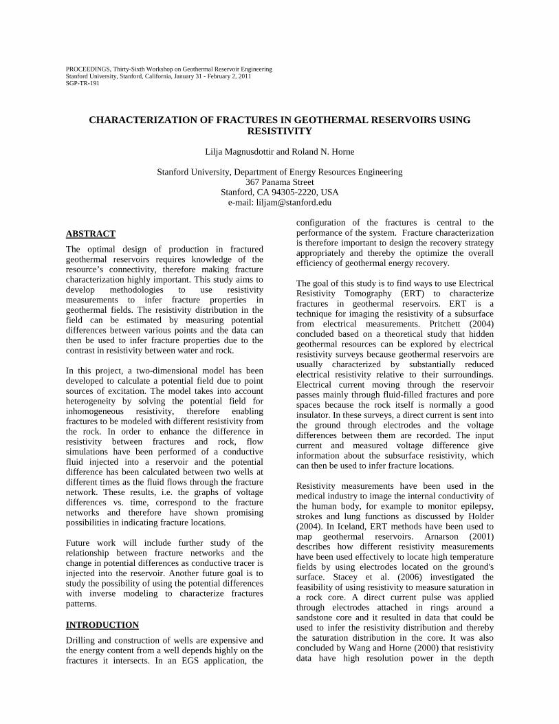
Finite Difference Equations in Two Dimensions The finite difference method is used to approximate the solution to the partial differential equation (Equation 5) using a point-discretization of the subsurface (Mufti, 1976). The computational domain is discretized into Nx×Ny blocks and the distance between two adjacent points on each block is h in the x-direction and l in the y-direction, as shown in Figure 1.

Figure 1: Computational domain, discretized into

blocks.

Taylor series expansion is used to approximate the derivatives of Equation 5 about a point (j,k) on the grid. Solving for the electric potential φ at that point gives,

[ ] [ ] 243

221

24

23

22

21

)1,()1,(

),1(),1(

),(hcclcc

hckjhckj

lckjlckjIhl

kj+++

⎥⎥⎦

⎤

⎢⎢⎣

⎡

−+++

−+++

=ϕϕ

ϕϕ

ϕ (6)

The parameters ci represent the conductivity averaged between two adjacent blocks and I [amp] is the current injected at point (j,k).

Iteration method In order to solve Equation 6 numerically and obtain the results for electrical potential φ at each point on the grid, the iteration method called Successive Over-Relaxation was used (Spencer and Ware, 2009). At first, a guess is made for φ(j,k) across the whole grid, and that guess is then used to calculate the right hand side (Rhs) of Equation 6 for each point and then a new set of values for φ(j,k) are calculated using the following iteration scheme,

nn Rhs ϕωωϕ )1(1 −+=+ (7) The multiplier ω is used to shift the eigenvalues so the iteration converges better than simple relaxation. The number ω is between 1 and 2, and when the computing region is rectangular the following equation can be used to get a reasonable good value for ω,

211

2

R−+=ω

(8) where:

2

coscos ⎟⎟⎠

⎞⎜⎜⎝

⎛⎟⎟⎠

⎞⎜⎜⎝

⎛+⎟⎠⎞

⎜⎝⎛

=NyNx

R

ππ

(9)

The natural Neumann boundary condition is used on

the outer boundaries in this project, i.e. 0=

∂∂

n

φ.

Results The resistivity model was first tested for a 160 × 160 m field with homogeneous resistivity as 1 Ωm. A current is set equal to 1 A at a point in the upper left corner, and as -1 A at the lower right corner. The potential distribution can be seen in Figure 2.

Figure 2: Potential distribution [V] for a

homogeneous resistivity field. The result for the homogeneous field is the same as given by the Partial Differential Equation (PDE) ToolboxTM in Matlab for this field. This toolbox in Matlab contains tools to preprocess, solve and postprocess partial differential equations in two dimensions (The MathWorks, 2003). However, the built in application for conductive media DC does not solve a potential field for inhomogeneous resistivity. In order to use the potential differences to distinguish between the rock and fractures, the model calculating the potential field must be able to take into account heterogeneity, as the model in this project does. Figure 3 shows the potential field where points on a line between the current injection points have resistivity 10,000 Ωm, while the rest of the field has resistivity 1 Ωm. The field is 160× 160 m as before, and a current equal to 1 A is injected in the upper left corner and -1 A in the lower right corner.

Figure 3: Potential distribution for an

inhomogeneous resistivity field. The potential field is higher than for a field with homogeneous resistivity (see Figure 2) and the electric field is higher at the high resistivity zone, as expected.

CHANGES IN POTENTIAL DIFFERENCE AS CONDUCTIVE FLUID IS INJECTED

Two different cases were explored in order to investigate the potential of using the resistivity model with conductive fluid to characterize fractures. In the first case, a very simple fracture network is modeled to explore how the potential field changes as the conductive fluid distributes through the network. In the second case, fractured rock is modeled in one corner of a reservoir and then later modeled in the opposite corner, in order to study the difference in potential field between those two cases and to further understand the relationship between the fracture networks and the voltage differences.

Case 1 A flow simulation was performed using the TOUGH2 reservoir simulator to see how a tracer, which increases the conductivity of the fluid, distributes after being injected into a reservoir. The simulation was carried out on a two dimensional grid with dimensions 1000 × 1000 × 10 m3. The fracture network can be seen in Figure 4, where the green blocks represent the fractures and wells are located at the upper left and lower right corner of the network.

Figure 4: A simple fracture network. The fracture blocks were given a porosity value of 0.65 and permeability value of 5×1011 md (5×10-4 m2) and the rest of the blocks were set to porosity 0.1 and permeability 1 md (10-15 m2). Closed or no-flow boundary conditions were used and one injector at upper left corner was modeled to inject water at 100 kg/s with enthalpy 100 kJ/kg, and a tracer at 0.01 kg/s with the same enthalpy. One production well at lower right corner was configured to produce at 100 kg/s.

The initial pressure was set to 10.13 MPa (100.13 bar), temperature to 150°C and initial tracer mass fraction was set to 10-9, because the simulator could not solve the problem with zero initial tracer mass fraction. Figure 5 illustrates how the tracer transfers through the fractures from the injector to the producer. After four days the tracer has distributed through the whole fracture network.

Figure 5: Tracer concentration after injecting for

two days. The results from the flow simulation were read into the resistivity model, so that the right conductivity values could be assigned for the reservoir. The conductivity value of each block depends on the tracer concentration in that block, and it is assumed that the tracer decreases the conductivity, for example a saline tracer. Table 1 shows how the conductivity values were assigned to different tracer concentration, X2. Table 1: Tracer concentration and corresponding

conductivity values. Tracer concentration Conductivity

[mohs-m-1] X2 <=1·10-9 2.4 1·10-9 <X2<=1·10-8 15 1·10-8 <X2<=1·10-7 20 1·10-7 <X2<=1·10-6 25 1·10-6 <X2<=1·10-5 30 X2>=1·10-5 35

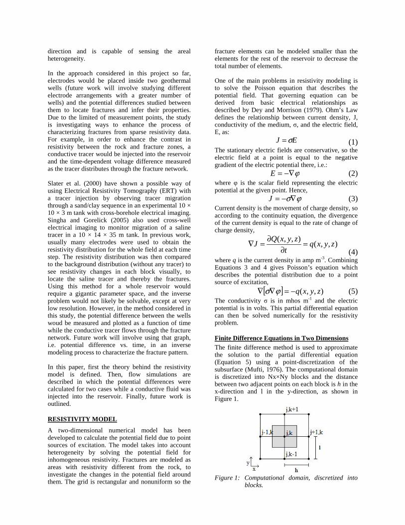
In the flow simulation the tracer concentration is calculated at different time steps and for each step the potential field is calculated using the resistivity model. Figure 6 shows the potential field for the same time step as shown in Figure 5, i.e. after injecting conductive fluid for two days.

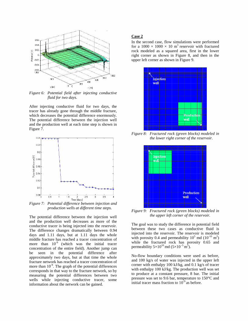
Figure 6: Potential field after injecting conductive

fluid for two days. After injecting conductive fluid for two days, the tracer has already gone through the middle fracture, which decreases the potential difference enormously. The potential difference between the injection well and the production well at each time step is shown in Figure 7.

Figure 7: Potential difference between injection and

production wells at different time steps. The potential difference between the injection well and the production well decreases as more of the conductive tracer is being injected into the reservoir. The difference changes dramatically between 0.94 days and 1.11 days, but at 1.11 days the whole middle fracture has reached a tracer concentration of more than 10-9 (which was the initial tracer concentration of the entire field). Another jump can be seen in the potential difference after approximately two days, but at that time the whole fracture network has reached a tracer concentration of more than 10-9. The graph of the potential differences corresponds in that way to the fracture network, so by measuring the potential differences between two wells while injecting conductive tracer, some information about the network can be gained.

Case 2 In the second case, flow simulations were performed for a 1000 × 1000 × 10 m3 reservoir with fractured rock modeled as a squared area, first in the lower right corner as shown in Figure 8, and then in the upper left corner as shown in Figure 9.

Figure 8: Fractured rock (green blocks) modeled in

the lower right corner of the reservoir.

Figure 9: Fractured rock (green blocks) modeled in

the upper left corner of the reservoir.

The goal was to study the difference in potential field between these two cases as conductive fluid is injected into the reservoir. The reservoir is modeled with porosity 0.4 and permeability 105 md (10-10 m2) while the fractured rock has porosity 0.65 and permeability 5×1010 md (5×10 -5 m2). No-flow boundary conditions were used as before, and 100 kg/s of water was injected in the upper left corner with enthalpy 100 kJ/kg, and 0.1 kg/s of tracer with enthalpy 100 kJ/kg. The production well was set to produce at a constant pressure, 8 bar. The initial pressure was set to 9.6 bar, temperature to 150°C and initial tracer mass fraction to 10-9 as before.

This time, the following equation was used to calculate the electrical conductivity, 1/ρw, of a NaCl water solution (Crain, 2010),

WsTw

⎟⎠⎞

⎜⎝⎛ +

=32

59

000,400ρ (10)

in order to define conductivity values in the resistivity model as NaCl tracer flows through the reservoir. T is the formation temperature (assumed to be 150°C) and Ws is the water salinity [ppm NaCl]. The resistivity for the rock before fluid had been injected was set as 100 Ωm for the fractured area (assuming fractures were filled with water) and as 2000 Ωm for the rest of the reservoir. Figures 10 and 11 show how the potential difference between the injector and the producer changes with time for the reservoirs shown in Figure 8 and 9.

Figure 10: Potential difference between injection and

production wells for reservoir in Figure 8.

Figure 11: Potential difference between injection and

production wells for reservoir in Figure 9.

The potential difference in the graph in Figure 10 drops very fast for the first 10 days, but then decreases more slowly when the tracer front has reached the fractured area. In the Figure 11, the potential difference drops slower, as the conductive fluid first fills up the fractured rock, modeled with much higher porosity then the rest of the reservoir. More cases need to be studied, and probably run for a longer time period, in order to understand the correspondence between the changes in potential differences and fracture networks. But these preliminary results indicate that different fracture properties give different potential differences between two wells, and could therefore be used to indicate fracture characteristics.

FUTURE WORK

The previous results have shown that the resistivity model has promising possibilities for fracture characterization, especially when used with a flow simulation of a conductive tracer. Future work will include solving the potential differences for more realistic fracture patterns. The main goal is to use the resistivity model and flow simulations with inverse modeling to estimate the dimensions and topology of a fracture network based on potential differences measured between wells. The objective is to develop a method that can be used to find where the fractures are located as well as the extent of their connectivity. In inverse modeling the results of actual observations are used to infer the values of the parameters characterizing the system under investigation. In this study, the output parameters are the potential difference between wells as a function of time and the input parameters will include the dimensions and orientations of the fractures between the wells. The objective function measures the difference between the model calculation (the calculated voltage difference between the wells) and the observed data (measured potential field between actual wells), as illustrated in Figure 12, and a minimization algorithm proposes new parameter sets that iteratively improve the match. After the inverse problem has been solved assuming the potential difference is known between wells all around the fractured area, the possibility of using fewer wells and different well arrangements will be studied to estimate the minimum number of wells necessary to solve the problem.

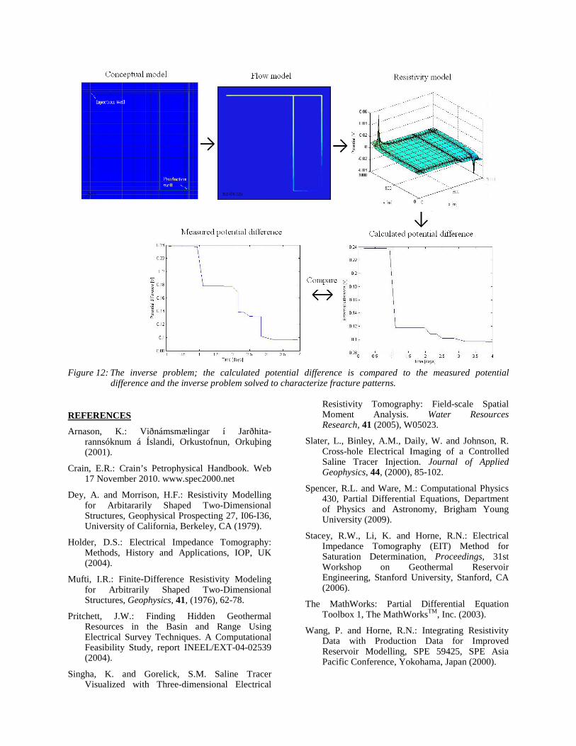
Figure 12: The inverse problem; the calculated potential difference is compared to the measured potential

difference and the inverse problem solved to characterize fracture patterns.

REFERENCES

Arnason, K.: Viðnámsmælingar í Jarðhita-rannsóknum á Íslandi, Orkustofnun, Orkuþing (2001).

Crain, E.R.: Crain’s Petrophysical Handbook. Web 17 November 2010. www.spec2000.net

Dey, A. and Morrison, H.F.: Resistivity Modelling for Arbitararily Shaped Two-Dimensional Structures, Geophysical Prospecting 27, I06-I36, University of California, Berkeley, CA (1979).

Holder, D.S.: Electrical Impedance Tomography: Methods, History and Applications, IOP, UK (2004).

Mufti, I.R.: Finite-Difference Resistivity Modeling for Arbitrarily Shaped Two-Dimensional Structures, Geophysics, 41, (1976), 62-78.

Pritchett, J.W.: Finding Hidden Geothermal Resources in the Basin and Range Using Electrical Survey Techniques. A Computational Feasibility Study, report INEEL/EXT-04-02539 (2004).

Singha, K. and Gorelick, S.M. Saline Tracer Visualized with Three-dimensional Electrical

Resistivity Tomography: Field-scale Spatial Moment Analysis. Water Resources Research, 41 (2005), W05023.

Slater, L., Binley, A.M., Daily, W. and Johnson, R. Cross-hole Electrical Imaging of a Controlled Saline Tracer Injection. Journal of Applied Geophysics, 44, (2000), 85-102.

Spencer, R.L. and Ware, M.: Computational Physics 430, Partial Differential Equations, Department of Physics and Astronomy, Brigham Young University (2009).

Stacey, R.W., Li, K. and Horne, R.N.: Electrical Impedance Tomography (EIT) Method for Saturation Determination, Proceedings, 31st Workshop on Geothermal Reservoir Engineering, Stanford University, Stanford, CA (2006).

The MathWorks: Partial Differential Equation Toolbox 1, The MathWorksTM, Inc. (2003).

Wang, P. and Horne, R.N.: Integrating Resistivity Data with Production Data for Improved Reservoir Modelling, SPE 59425, SPE Asia Pacific Conference, Yokohama, Japan (2000).