CHARACTERIZATION OF DYNAMIC AND STATIC MECHANICAL BEHAVIOR OF POLYETHERIMIDE by...
100
CHARACTERIZATION OF DYNAMIC AND STATIC MECHANICAL BEHAVIOR OF POLYETHERIMIDE by NATHAN J. MUTTER B.S. University of Central Florida, 2010 A thesis submitted in partial fulfillment of the requirements for the degree of Master of Science in Mechanical Engineering in the Department of Mechanical, Materials, and Aerospace Engineering in the College of Engineering and Computer Science at the University of Central Florida Orlando, Florida Spring Term 2012
Transcript of CHARACTERIZATION OF DYNAMIC AND STATIC MECHANICAL BEHAVIOR OF POLYETHERIMIDE by...
CHARACTERIZATION OF DYNAMIC AND STATIC MECHANICAL BEHAVIOR OF
POLYETHERIMIDE
by
NATHAN J. MUTTER
B.S. University of Central Florida, 2010
A thesis submitted in partial fulfillment of the requirements
for the degree of Master of Science in Mechanical Engineering
in the Department of Mechanical, Materials, and Aerospace Engineering
in the College of Engineering and Computer Science
at the University of Central Florida
Orlando, Florida
Spring Term
2012

ii
© 2012 Nathan Mutter

iii
ABSTRACT
Polymers are increasingly being used in engineering designs due to their favorable
mechanical properties such as high specific strength, corrosive resistance, manufacturing
flexibility. The understanding of the mechanical behavior of these polymers under both static
and dynamic loading is critical for their optimal implementation in engineering applications.
One such polymer utilized in a wide variety of applications from medical instrumentation to
munitions is Polyetherimide, referred to as Ultem. This thesis characterizes both the static and
dynamic mechanical behavior of Ultem 1000 through experimental methods and numerical
simulations. Standard compression experiments were conducted on and MTS test frame to
characterize the elastic-plastic behavior of Ultem 1000 under quasi-static conditions. The
dynamic response of the material was investigated at very high strain rates using a custom built
miniaturized Kolsky bar apparatus. The smaller Kolsky bar configuration was chosen over the
conventional Kolsky device to increase the maximum capable strain rates and to reduce common
experimental problems such as wave dispersion, friction, and stress equilibrium. Since a
universal test standard for this apparatus is not available, the details of the design, construction,
and experimental procedures of this device are provided. The results of the high strain rate
testing revealed a bilinear relationship between the material yield stress and strain rate. This
relationship was modeled using the Ree-Eyring two stage activation process equation.

iv
ACKNOWLEDGMENTS
I would like to take this time to thank a number of people whose support was integral to
the completion of this study. Most importantly, I would like to express my gratitude for my
thesis chair, Dr. Ali P. Gordon, whose skillful guidance, wisdom, and energy facilitated the most
meaningful learning experiences throughout my undergraduate and graduate career. Dr. Gordon
has been my advisor for over four years during which I have grown tremendously both
personally and professionally. I am indebted to Dr. Gordon for his years of mentorship and
support. My other thesis committee members, Dr. Cheryl Xu and Dr. Seetha Raghavan, deserve
special thanks for their insightful inputs throughout the course of this study. I am also thankful
for the experienced consultation of Dr. Jamie Kimberley of Johns Hopkins University who
offered invaluable advice during the design phase of the Kolsky bar device.
I would also like to individually thank the undergraduate and graduate researchers within
the Mechanics of Materials Research Group (MOMRG) for their assistance. Chris Harrison was
instrumental in the design and construction of the Kolsky bar device. Bryan Zuanetti expertly
fabricated all of the specimens used in the Kolsky bar experiments. Justin Karl frequently
provided technical advice regarding the electronic components and data acquisition systems of
the Kolsky bar device. Scott Keller continually shared his expertise in mechanical testing which
improved the accuracy and reliability of the Kolsky bar experiments. There are many other
students, faculty, and staff within the Mechanical, Materials, and Aerospace Engineering
department at UCF who have aided me along the way to whom I am greatly appreciative.
Finally, I would like to thank my wife and my family for their continual support and
encouragement throughout my educational endeavors.
v
TABLE OF CONTENTS
LIST OF FIGURES ...................................................................................................................... vii
LIST OF TABLES .......................................................................................................................... x
LIST OF NOMENCLATURE ....................................................................................................... xi
1. INTRODUCTION AND MOTIVATION .................................................................................. 1
2. BACKGROUND ........................................................................................................................ 4
2.1 Kolsky Bar Background ........................................................................................................ 4
2.1.1 Kolsky Bar Theory ......................................................................................................... 4
2.1.2 Kolsky Bar Evolution .................................................................................................... 7
2.2 Material Background ............................................................................................................ 9
2.2.1 Polyetherimide ............................................................................................................... 9
2.2.2 Rate Dependent Polymer Characterization .................................................................. 11
3. DESKTOP KOLSKY BAR DESIGN, CONSTRUCTION, AND CALIBRATION ............... 17
3.1 Design ................................................................................................................................. 17
3.2 Construction ........................................................................................................................ 20
3.3 Calibration........................................................................................................................... 29
3.3.1 Strain Gauge Gain Calibration ..................................................................................... 30
3.3.2 Strain Pulse Calibration ............................................................................................... 31
4. EXPERIMENTAL SETUP ....................................................................................................... 35

vi
4.1 Specimen Preparation ......................................................................................................... 35
4.2 Quasi-Static and Medium Strain Rate Compression Experiments ..................................... 36
4.3 Kolsky Bar Experiments ..................................................................................................... 38
5. EXPERIMENTAL RESULTS.................................................................................................. 41
5.1 Quasi-Static and Medium Strain Rate Compression Results .............................................. 41
5.2 Kolsky Bar Results ............................................................................................................. 42
5.2.1 Data Analysis ............................................................................................................... 42
5.2.2 Experimental Results ................................................................................................... 50
6. DISCUSSION ........................................................................................................................... 58
7. CONCLUSION AND FUTURE WORK ................................................................................. 61
7.1 Conclusions ......................................................................................................................... 61
7.2 Future Work ........................................................................................................................ 61
APPENDIX A: TEST HARDWARE ........................................................................................... 64
APPENDIX B: STRIKER BAR VELOCITY LABVIEW VI ..................................................... 71
APPENDIX C: DATA PROCESSING CODE............................................................................. 73
APPENDIX D: SPECIMENS AND TEST DATA ...................................................................... 76
REFERENCES ............................................................................................................................. 84
vii
LIST OF FIGURES
Figure 1. Guided projectile application of Ultem 1000 .................................................................. 2
Figure 2. Schematic of Kolsky bar apparatus ................................................................................. 5
Figure 3. Example of incident, reflected, and transmitted pulses ................................................... 6
Figure 4. Chemical composition of Ultem 1000 [Pecht, 1994] ...................................................... 9
Figure 5. Schematic of amorphous polymer chains ...................................................................... 10
Figure 6. Quasi-static compressive stress-strain curve of Ultem 1000 ......................................... 12
Figure 7. Rate dependent stress-strain curves for PMMA [Chou, 1973] ...................................... 14
Figure 8. Rate dependent stress strain curves for PC [Siviour, 2005] .......................................... 14
Figure 9. Strain rate versus peak stress for PC [Siviour, 2005] .................................................... 15
Figure 10. Desktop Kolsky bar apparatus ..................................................................................... 21
Figure 11. Air delivery system...................................................................................................... 22
Figure 12. Alignment stanchion .................................................................................................... 23
Figure 13. Interface between impact and transmission bars ......................................................... 24
Figure 14. Momentum trapping system ........................................................................................ 25
Figure 15. Striker bar assembly .................................................................................................... 26
Figure 16. Bonded terminal and strain gauge configuration (a) and reinforced gauge (b) ........... 27
Figure 17. Strain gauge amplification circuit ............................................................................... 28
Figure 18. System signal flow chart ............................................................................................. 29
Figure 19. Strain gauge gain calibration plot ................................................................................ 31
Figure 20. Pulses for bars together calibration ............................................................................. 32
Figure 21. Calibrated pulses for bars together .............................................................................. 34
viii
Figure 22. Micrograph of Ultem 1000 test specimen ................................................................... 36
Figure 23. Specimen polishing jig ................................................................................................ 36
Figure 24. Test configuration used in quasi-static testing ............................................................ 37
Figure 25. Lubrication applied to the impact bar .......................................................................... 39
Figure 26. Specimen in Kolsky bar experiment ............................................................................ 40
Figure 27. Quasi-static stress strain curves ................................................................................... 42
Figure 28. Post-processed strain pulses from example Kolsky bar experiment ........................... 45
Figure 29. Synchronized strain pulses .......................................................................................... 46
Figure 30. Stress equilibrium comparison graph .......................................................................... 46
Figure 31. Stress equilibrium verification graph .......................................................................... 47
Figure 32. Strain rate versus time ................................................................................................. 48
Figure 33. Specimen strain versus time ........................................................................................ 49
Figure 34. Specimen stress strain curve ........................................................................................ 50
Figure 35. Ultem 1000 specimen before and after Kolsky bar experiment .................................. 51
Figure 36. Stress-strain curves of Ultem 1000 at various strain rates .......................................... 52
Figure 37. Ultem 1000 yield stress versus strain rate ................................................................... 53
Figure 38. Ree-Erying model fit to experimental data ................................................................. 54
Figure 39. Ramberg-Osgood model fit of experimental data ....................................................... 55
Figure 40. Ramberg-Osgood model for various strain rates ......................................................... 56
Figure 41. Rate dependence of hardening coefficient, n .............................................................. 57
Figure 42. Rate dependence of Ramberg-Osgood coefficient, K ................................................. 57
Figure 43. Launch tube drawing (dimensions in inches) .............................................................. 65

ix
Figure 44. Launch tube alignment block drawing (dimensions in inches) ................................... 66
Figure 45. LH1 lens holder drawing (Thor Labs) ......................................................................... 67
Figure 46. TR3 lens mount post drawing (Thor Labs) ................................................................. 68
Figure 47. PH2 post holder (Thor Labs) ....................................................................................... 69
Figure 48. Striker bar bushing drawing (dimensions are in inches) ............................................. 70
Figure 49. LabVIEW VI block diagram (a) and front panel (b) ................................................... 72
Figure 50. True stress-strain curve for specimen 100 ................................................................... 78
Figure 51. True stress-strain curve for specimen 101 ................................................................... 78
Figure 52. True stress-strain curve for specimen 102 ................................................................... 79
Figure 53. True stress-strain curve for specimen 103 ................................................................... 79
Figure 54. True stress-strain curve for specimen 104 ................................................................... 80
Figure 55. True stress-strain curve for specimen 107 ................................................................... 80
Figure 56. True stress-strain curve for specimen 108 ................................................................... 81
Figure 57. True stress-strain curve for specimen 109 ................................................................... 81
Figure 58. True stress-strain curve for specimen 110 ................................................................... 82
Figure 59. True stress-strain curve for specimen 111 ................................................................... 82
Figure 60. True stress-strain curve for specimen 112 ................................................................... 83
Figure 61. True stress-strain curve for specimen 113 ................................................................... 83
x
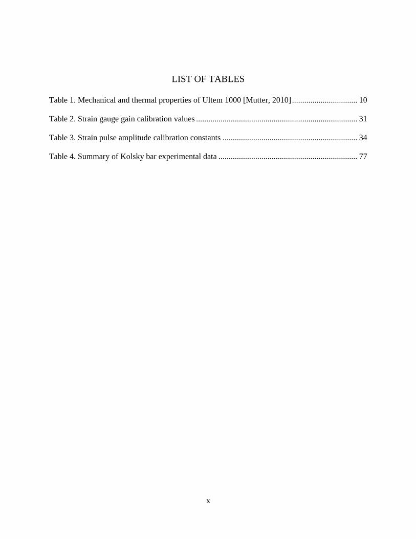
LIST OF TABLES
Table 1. Mechanical and thermal properties of Ultem 1000 [Mutter, 2010] ................................ 10
Table 2. Strain gauge gain calibration values ............................................................................... 31
Table 3. Strain pulse amplitude calibration constants .................................................................. 34
Table 4. Summary of Kolsky bar experimental data .................................................................... 77

xi
LIST OF NOMENCLATURE
True strain
Strain rate
, , Incident, reflected, and transmitted strain pulses
θ Absolute temperature
, Density of bar and specimen
σ True stress
σy Yield stress
τ Ring up period
A1, A2 Ree-Eyring coefficients
Ab, As Area of bar and specimen
C1, C2 Ree-Eyring coefficients
Cb, Cs Elastic wave speed of bar material and specimen
Db, Ds Diameter of bar and specimen
e Engineering stress
Eb, Es Elastic modulus of bar and specimen
Lb, Ls, Lst Length of impact/transmission bar, specimen, and striker bar
Q1, Q2 Activation energies
R Universal gas constant
T Period of incident pulse
Velocity of striker bar

1
1. INTRODUCTION AND MOTIVATION
It is well known that the mechanical properties of many engineering materials are
dependent on the rate of deformation to which the material is subjected. This dependence is
more pronounced for certain materials such as polymers and at very high strain rates
(102
– 104 s
-1). Due to the increase of use of polymers in many engineering designs, it is
desirable to accurately characterize the behavior of these polymers at very high strain rates. One
widely employed method of experimentally determining the high strain rate response of
materials is by using a Split Hopkinson Pressure Bar (SHPB) or Kolsky bar device. Such
pressure bar devices have been used by various researchers since the pioneering work of Bertram
Hopkinson in 1914 [Hopkinson, 1914]. The present work investigates the high strain rate
mechanical behavior of Polyetherimide, also referred to as Ultem, through use of a miniaturized
Split Hopkinson Pressure Bar (mSHPB). Ultem is a thermoplastic which is used in many static
and dynamic engineering applications throughout various industries due to its high strength to
weight ratio and other favorable characteristics, but has yet to be analyzed under dynamic
conditions. In the defense industry, Ultem is employed in guided projectile designs, illustrated in
Figure 1, where circular Ultem plates are designed to fail in a predictable manner under dynamic
axisymmetric pressure.

2
Figure 1. Guided projectile application of Ultem 1000
Although Kolsky bars have been successfully used for decades, the devices are not
commercially available and there is no formal standardized test method to guide researchers on
the proper experimental setup, procedure, or data analysis. Furthermore, only a small fraction of
the available literature on Kolsky bar testing is related to the miniaturized version of the Kolsky
bars, which possess many advantages over the full-scale Kolsky bar system. As such, this thesis
is also intended to serve as a detailed guide on the design, construction, calibration, and
experimental procedure for a custom built miniaturized Kolsky bar device. All of the needed
parts and materials are listed along with detailed engineering drawings of the various custom
made components. The goals of this project were to design and fabricate an accurate Kolsky bar
system within a relatively modest budget, characterize the strain rate dependence of Ultem 1000
under compression, and to contribute to the existing body of literature a guide for research
groups to be able to design and construct their own Kolsky bar device more efficiently.
A review of the literature regarding the development of the Kolsky bar device, its
improvements throughout the years, and its application to the characterization of polymers is
given in Chapter 2. Chapter 3 covers the design, construction, and calibration of the
miniaturized Kolsky bar system. The experimental setup and specific procedures for the quasi-

3
static and high strain rate experiments are provided in Chapter 4. The results of the experiments
are presented in Chapter 5 and discussed in Chapter 6. Finally, Chapter 7 contains the
conclusions as well as planned future work regarding the miniaturized Kolsky bar system.
Appendix A contains a detailed bill of materials and engineering drawings for the construction of
the Kolsky bars. The codes developed for measuring the striker velocity (LabVIEW) and
processing the experimental data (MATLAB) are provided in Appendix B and Appendix C,
respectively. Photographs of the specimens used in the experiments as well as experimental data
are provided in Appendix D.

4
2. BACKGROUND
2.1 Kolsky Bar Background
2.1.1 Kolsky Bar Theory
The original Kolsky bar device, constructed in 1949, was designed to subject specimens
to high rate compression deformation. Typically, a compression Kolsky bar apparatus is
comprised of three bars, each of the same material and diameter ranging between 10 and 25 mm.
The three bars are referred to as the striker bar, the impact bar, and the transmission bar and are
shown schematically in Figure 2. Prior to the start of an experiment, the specimen is sandwiched
between the impact and transmission bars. Then the striker bar is given a velocity ( ), usually
by the expansion of compressed gas, and will strike the impact bar sending a compressive pulse
through the impact bar. This compressive pulse, known as the incident pulse ( ), will travel
through the impact bar at the elastic wave speed as defined by
(1)
where is the elastic modulus and is the density of the bar material. The magnitude of this
incident pulse is determined by
(2)
and the width of the pulse, T, is
(3)
5
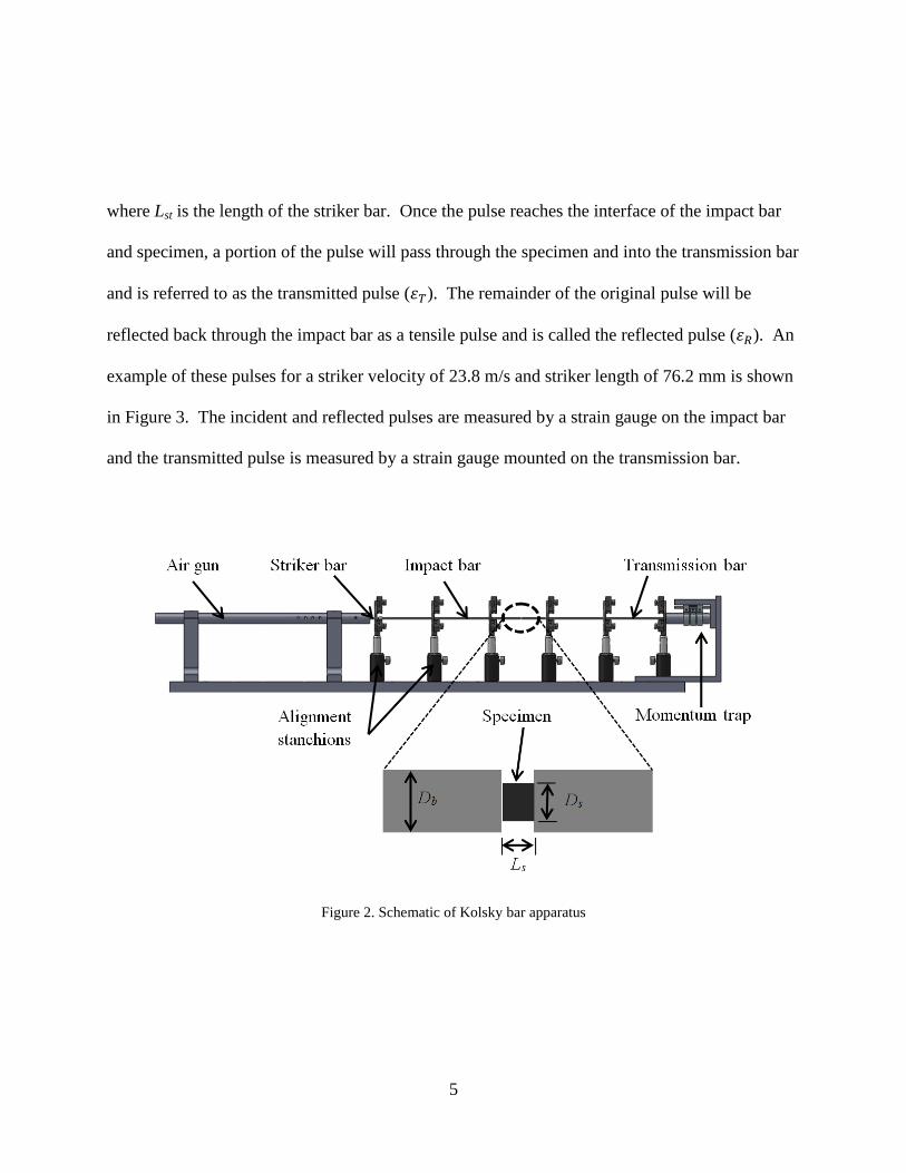
where Lst is the length of the striker bar. Once the pulse reaches the interface of the impact bar
and specimen, a portion of the pulse will pass through the specimen and into the transmission bar
and is referred to as the transmitted pulse ( ). The remainder of the original pulse will be
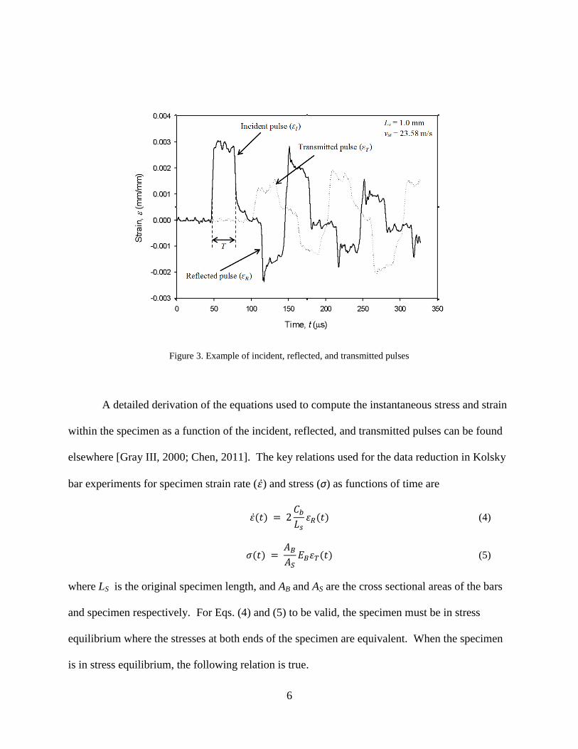
reflected back through the impact bar as a tensile pulse and is called the reflected pulse ( ). An
example of these pulses for a striker velocity of 23.8 m/s and striker length of 76.2 mm is shown
in Figure 3. The incident and reflected pulses are measured by a strain gauge on the impact bar
and the transmitted pulse is measured by a strain gauge mounted on the transmission bar.
Figure 2. Schematic of Kolsky bar apparatus
6
Figure 3. Example of incident, reflected, and transmitted pulses
A detailed derivation of the equations used to compute the instantaneous stress and strain
within the specimen as a function of the incident, reflected, and transmitted pulses can be found
elsewhere [Gray III, 2000; Chen, 2011]. The key relations used for the data reduction in Kolsky
bar experiments for specimen strain rate ( ) and stress (σ) as functions of time are
(4)
(5)
where LS is the original specimen length, and AB and AS are the cross sectional areas of the bars
and specimen respectively. For Eqs. (4) and (5) to be valid, the specimen must be in stress
equilibrium where the stresses at both ends of the specimen are equivalent. When the specimen
is in stress equilibrium, the following relation is true.
7
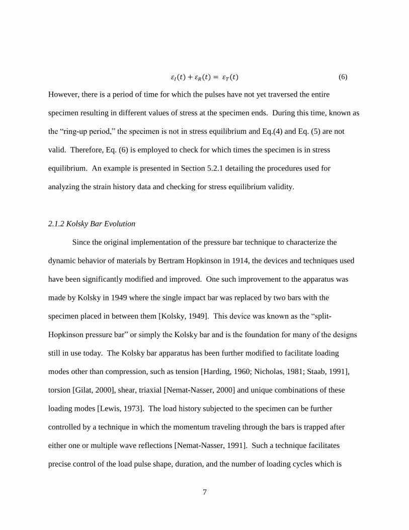
(6)
However, there is a period of time for which the pulses have not yet traversed the entire
specimen resulting in different values of stress at the specimen ends. During this time, known as
the “ring-up period,” the specimen is not in stress equilibrium and Eq.(4) and Eq. (5) are not
valid. Therefore, Eq. (6) is employed to check for which times the specimen is in stress
equilibrium. An example is presented in Section 5.2.1 detailing the procedures used for
analyzing the strain history data and checking for stress equilibrium validity.
2.1.2 Kolsky Bar Evolution
Since the original implementation of the pressure bar technique to characterize the
dynamic behavior of materials by Bertram Hopkinson in 1914, the devices and techniques used
have been significantly modified and improved. One such improvement to the apparatus was
made by Kolsky in 1949 where the single impact bar was replaced by two bars with the
specimen placed in between them [Kolsky, 1949]. This device was known as the “split-
Hopkinson pressure bar” or simply the Kolsky bar and is the foundation for many of the designs
still in use today. The Kolsky bar apparatus has been further modified to facilitate loading
modes other than compression, such as tension [Harding, 1960; Nicholas, 1981; Staab, 1991],
torsion [Gilat, 2000], shear, triaxial [Nemat-Nasser, 2000] and unique combinations of these
loading modes [Lewis, 1973]. The load history subjected to the specimen can be further
controlled by a technique in which the momentum traveling through the bars is trapped after
either one or multiple wave reflections [Nemat-Nasser, 1991]. Such a technique facilitates
precise control of the load pulse shape, duration, and the number of loading cycles which is
8
critical for dynamic recovery experiments. Furthermore, material properties other than the
stress-strain response have been investigated under high strain rate conditions such as dynamic
indentation and fracture toughness properties [Klepaczko, 1980].
The Kolsky bar apparatus has also been modified to test a wide range of materials
including concrete [Zhao, 1998], ceramics [Subhash, 2000], and soft materials such as foam, and
polymers [Gray III and Blumenthal, 2000]. The testing of soft or low impedance materials
requires special considerations, especially when using polymer materials for the bars, and a
detailed discussion on the topic is provided in [Gray III and Blumenthal, 2000]. Researchers
have also developed methods to heat or cool the specimen just prior to testing so the dual effects
of temperature and strain rate can be investigate [Frantz, 1984; Gray, 1997].
In addition to modifications made to the physical device, improvements have been made
to the data acquisition and analysis processes for increased accuracy in experimental results.
Since in an actual Kolsky bar experiment a longitudinal pulse is traveling through a 3D rod, a
phenomenon known as wave dispersion was found to adversely affect the accuracy of the
collected data [Davies, 1948]. Pochhammer [Pochhammer, 1876] and Chree [Chree, 1889],
were the first to solve for the propagation of waves through cylindrical bars, but Davies [Davies,
1948] was the first to apply their solutions to the Kolsky bar technique. Since then various
researchers have developed mathematical techniques to correct the measured pulses for wave
dispersion [Follansbee, 1983; Gong, 1990; Gorham, 1983; Lifshitz, 1994; Tyas, 2005; Yew,
1978].

9
2.2 Material Background
2.2.1 Polyetherimide
The material under investigation, Ultem 1000, is an amorphous thermoplastic without
fillers or other fiber reinforcements. Ultem 1000 is composed of repeating units of C37H24O6N2
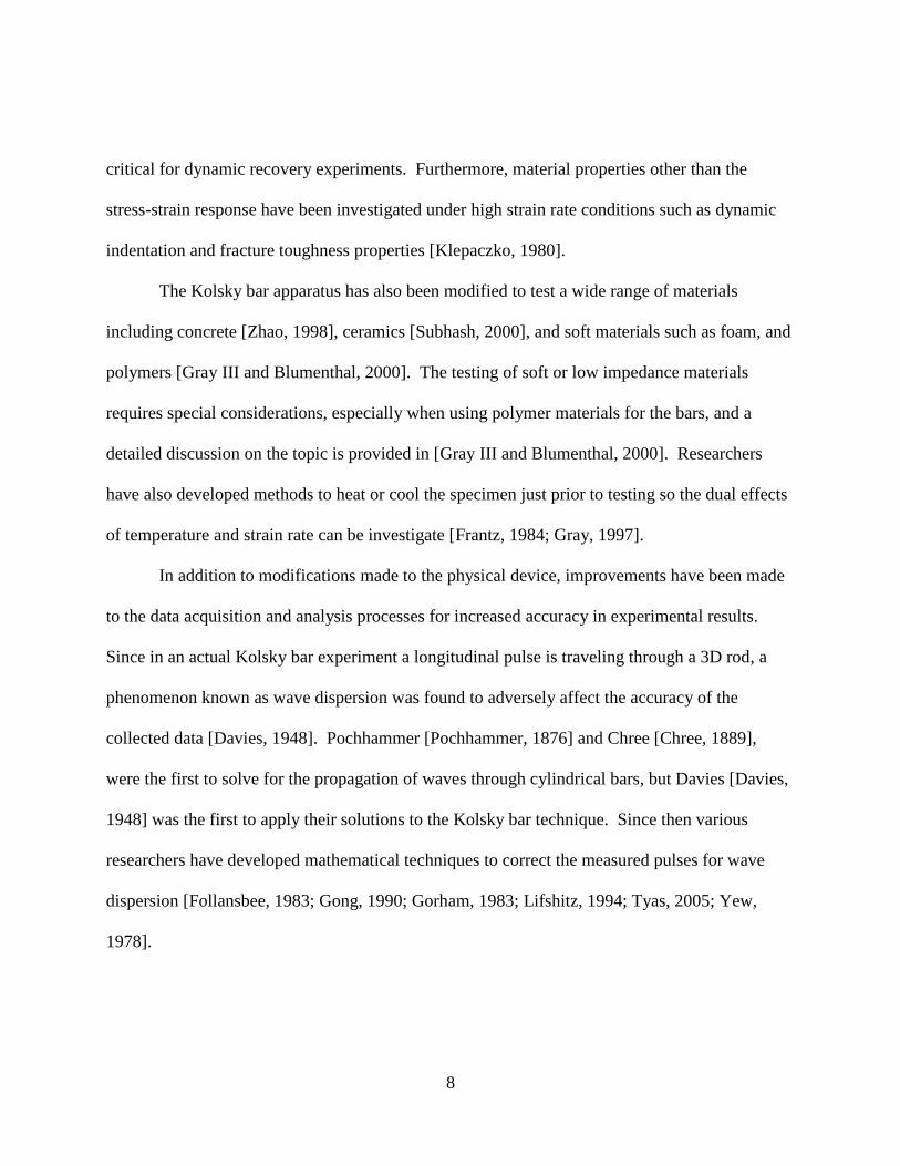
which is shown in Figure 4. Amorphous refers to the random orientation of polymer chains
shown schematically in Figure 5. The molecular organization and interaction of these chains
determines the mechanical response of polymers much like the crystalline structures in metallic
materials. Since Ultem 1000 is used in a range of applications ranging from aerospace to
medical industries, the quasi-static mechanical properties as well as fatigue, creep, and wear
properties have been previously characterized [Bijwe, 1990; Facca, 2006; Smmazcelik, 2008;
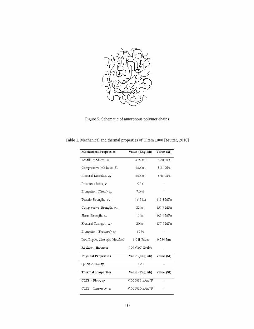
Stokes, 1988; Tou, 2007]. Selected mechanical and thermal properties of Ultem 1000 are
provided in Table 1.
Figure 4. Chemical composition of Ultem 1000 [Pecht, 1994]
10
Figure 5. Schematic of amorphous polymer chains
Table 1. Mechanical and thermal properties of Ultem 1000 [Mutter, 2010]

11
2.2.2 Rate Dependent Polymer Characterization
The rate-dependent behavior of polymers has received relatively little attention in
comparison to engineering metals over the years; however, since plastic materials are replacing
metals in many engineering designs, the dynamic stress-strain response of these materials is of
considerable interest. A brief review of past investigations of polymer rate dependency is
presented here, but the discussion is limited to amorphous polymers as their temperature and rate
dependent mechanical response differ from crystalline or semicrystaline polymers and since the
candidate material (Ultem 1000) is an amorphous polymer.
Before the strain rate effects on material behavior can be understood, it is enlightening to
review the typical quasi-static response of an amorphous polymer and the underlying molecular
interactions. Also, it is helpful to clarify the definitions of some of the mechanical properties as
determined from a stress-strain curve since these definitions differ from those commonly used in
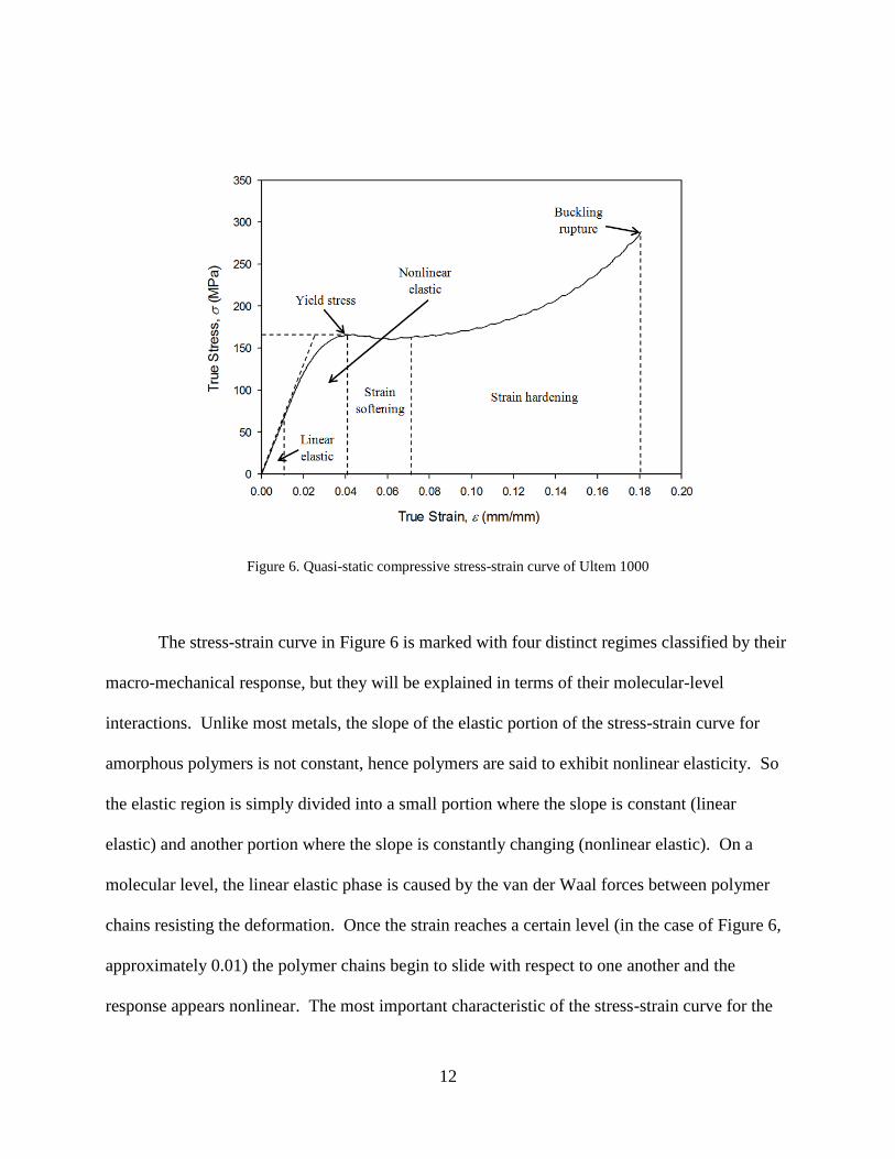
metals. To illustrate, a quasi-static compressive stress strain curve of Ultem 1000 is shown in
Figure 6.
12
Figure 6. Quasi-static compressive stress-strain curve of Ultem 1000
The stress-strain curve in Figure 6 is marked with four distinct regimes classified by their
macro-mechanical response, but they will be explained in terms of their molecular-level
interactions. Unlike most metals, the slope of the elastic portion of the stress-strain curve for
amorphous polymers is not constant, hence polymers are said to exhibit nonlinear elasticity. So
the elastic region is simply divided into a small portion where the slope is constant (linear
elastic) and another portion where the slope is constantly changing (nonlinear elastic). On a
molecular level, the linear elastic phase is caused by the van der Waal forces between polymer
chains resisting the deformation. Once the strain reaches a certain level (in the case of Figure 6,
approximately 0.01) the polymer chains begin to slide with respect to one another and the
response appears nonlinear. The most important characteristic of the stress-strain curve for the

13
purposes of the present work is the yield stress denoted in Figure 6. The yield stress defined for
amorphous polymers is the local maximum in stress just after the elastic portions where the
material deforms or flows without an increase in stress. This definition differs from that used in
the analysis of metallic materials, but is widely accepted for polymers. The third phase (strain
softening) has been the source of some debate as to whether it is caused by a local temperature
rise [Marshall, 1954] or a permanent rearrangement of polymer chains with respect to one
another [Brown, 1968]. However, for quasi-static testing conditions, the time scale needed for
the temperature to equilibrate is smaller than the loading rate and the strain softening can be
attributed to a permanent molecular rearrangement [Vincent, 1960]. Lastly, the strain hardening
phase is a result of the once randomly oriented polymer chains aligning themselves in such a way
requiring increased levels of stress for continued deformation.
Now that the quasi-static response is well defined, a brief review of the rate-dependent
investigations of amorphous polymers is presented. The first researcher credited for conducting
such investigations is Chou et al. [Chou, 1973]. He employed a Kolsky bar device and custom
medium-strain rate apparatus to subject polymethylmethacrylate (PMMA), cellulose acetate
butyrate (CAB), polypropylene, and nylon 6-6 specimens to strain rates ranging from 10-4
to 103
s-1
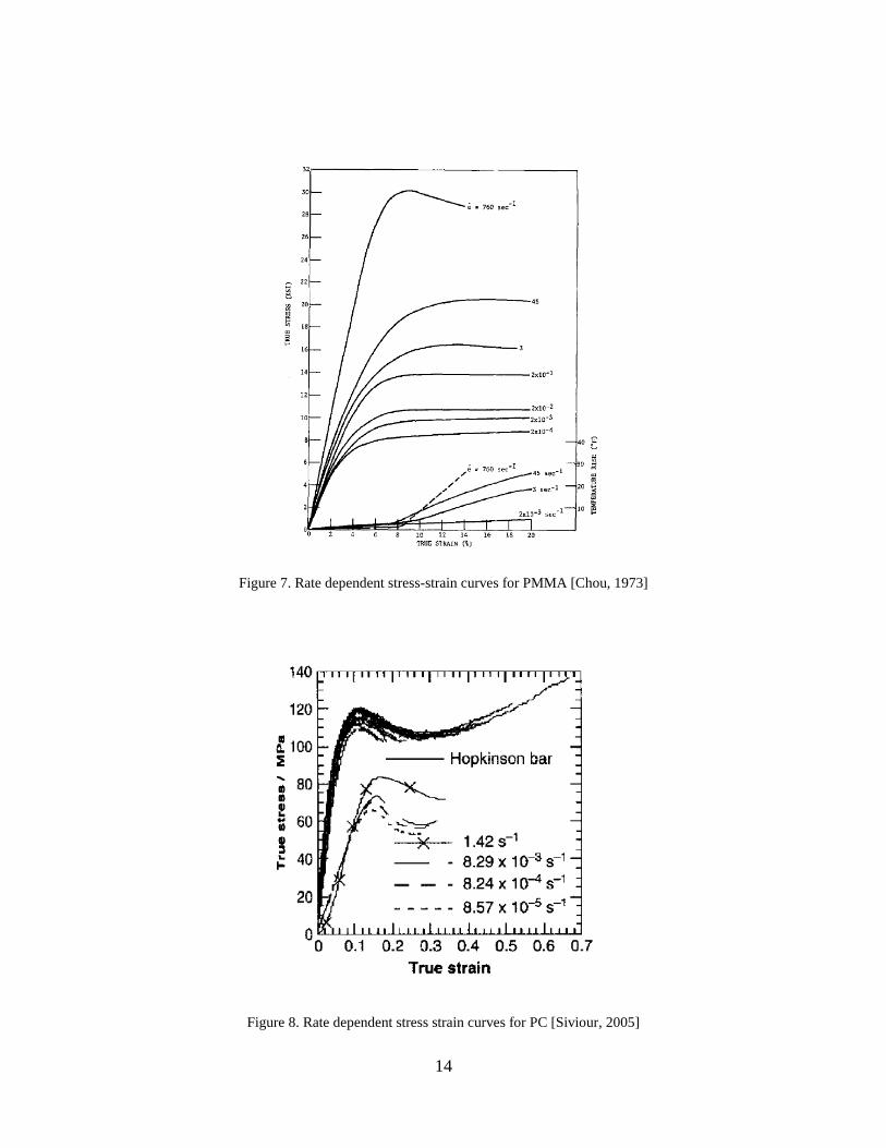
. Some of the results from this work are shown in Figure 7 for PMMA. As expected, the yield
stress exhibited by the material increases with increasing strain rate ( ). Another example of this
relationship between yield stress and strain rate is in Figure 8 where the rate dependent stress
strain curves for polycarbonate (PC) are shown for rates from 10-5
to 104 s
-1.
14
Figure 7. Rate dependent stress-strain curves for PMMA [Chou, 1973]
Figure 8. Rate dependent stress strain curves for PC [Siviour, 2005]

15
Furthermore, Walley and Field and others [Field, 1994; Walley, 1989; Walley, 1991]
investigated a wide range of polymers, both at room temperature and elevated temperature, from
rates of 10-2
to 104 s
-1. They, too, observed the relationship between the yield stress and the
strain rate, but went further to classify materials into three groups based on the type of
relationship observed between yield stress and log( ). The three groups are (1) materials that
exhibit a linear relationship between yield stress and log( ), (2) materials that exhibit a bilinear
relationship between yield stress and log( ), and (3) materials that exhibit a decrease in yield at
approximately 103 s
-1 [Siviour, 2005]. An example of the bilinear dependence on log( ) is
shown in Figure 9 for PC tested at room temperature.
Figure 9. Strain rate versus peak stress for PC [Siviour, 2005]
Unlike in the quasi-static case, the dynamic response of amorphous polymers requires the
careful examination of both the temperature rise due to rapid plastic deformation and the
16
molecular rearrangement of polymer chains. The rate dependence of yield stress in amorphous
polymers has been successfully modeled by the Eyring activation theory [Eyring, 1936] by many
investigators [Bauwens-Crowet, 1969] for strain rates up to 10-2
s-1
. This model predicts a linear
relationship between yield stress and log( ) which fit the experimental data satisfactorily for
Bauwens and others at the time. However, for the materials that exhibit a bilinear relationship
between yield stress and log( ), a modified model known as the Ree-Eyring equation was
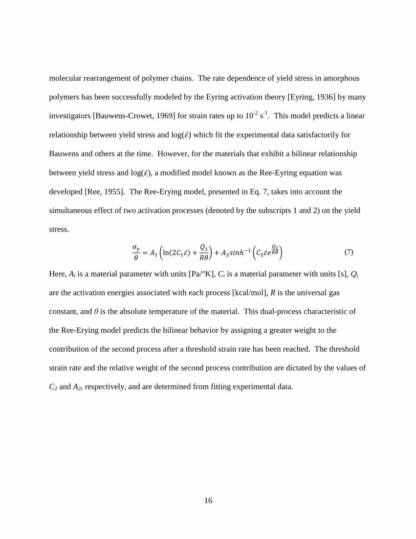
developed [Ree, 1955]. The Ree-Erying model, presented in Eq. 7, takes into account the
simultaneous effect of two activation processes (denoted by the subscripts 1 and 2) on the yield
stress.
(7)
Here, Ai is a material parameter with units [Pa/°K], Ci is a material parameter with units [s], Qi
are the activation energies associated with each process [kcal/mol], R is the universal gas
constant, and θ is the absolute temperature of the material. This dual-process characteristic of
the Ree-Erying model predicts the bilinear behavior by assigning a greater weight to the
contribution of the second process after a threshold strain rate has been reached. The threshold
strain rate and the relative weight of the second process contribution are dictated by the values of
C2 and A2, respectively, and are determined from fitting experimental data.

17
3. DESKTOP KOLSKY BAR DESIGN, CONSTRUCTION, AND
CALIBRATION
Although Kolsky bars have been used successfully for decades, there exists no
standardized (ASTM, ISO, etc.) method for designing, constructing, and carrying out Kolsky bar
experiments. This is because the design of the device is highly dependent on the specific
application and because there is still much on-going research on how to solve many of the
complications associated with this type of testing. Perhaps the most extensive set of guidelines
are found in the ASM Handbook [Gray III, 2000] and by Chen and Song [Chen, 2011]. Even in
these relatively comprehensive works, numerous references are made to other works which focus
on specific technical issues such as wave dispersion, lubrication methods, and momentum
trapping techniques. A discussion is presented in this chapter on the methodologies followed to
design and construct the miniaturized Kolsky bar used for the experiments in the present work.
Detailed explanations are given regarding design choices and fabrication techniques with the
goal of providing a template for others to build and modify Kolsky bar devices. Additionally, an
approach to modify the current Kolsky bar design to test other classes of materials, such as
metals, is provided at the end of the chapter.
3.1 Design
Configuring the desktop Kolsky bar device is a process which is dependent on the
specimen strength, length scale, strain rate, loading mode, and environment. The Kolsky bar
device constructed for the present work is much smaller than the typical setup and is referred to
as a miniaturized or desktop Kolsky bar. The overall length of the desktop apparatus is

18
approximately 1 meter compared to approximately 6 meters for a full-scale setup and the bar
diameters are 3.175 mm compared to the conventional diameter of 10-25 mm [Gray III, 2000].
There are numerous advantages to miniaturizing the Kolsky bars such as increasing the upper
limit on strain rate, and reducing the negative effects of wave dispersion, friction, and inertia in
the bars and specimen. A thorough investigation of these benefits was conducted by Jia and
Ramesh [Jia, 2004].
The primary design consideration is the yield strength and stiffness of the candidate
material as this will dictate the choice of bar material that must be used. The derivation of Eqs.
(4) and (5) requires that the impact and transmission bars deform elastically. Hence, the yield
strength of the bar material must be greater than the stress generated by the initial impact of the
striker and impact bars which is given by
(8)
In addition to the bar strength, the bar stiffness must be considered with respect to the
stiffness of the materials to be tested. If the bars are too stiff in comparison to the specimen
material, the sensitivity of the output signals from the gauges will be reduced and complications
in data reduction may arise due to the low signal magnitude. To increase the resolution of the
output signals, investigators have used low impedance bar materials such as titanium alloys
[Field, 2004], aluminum alloys [Chen, 1999], and polymeric materials [Sawas, 1998; Wang,
1994; Zhao, 1997]. The viscoelastic behavior of polymeric bar materials complicates the data
analysis because the simple linear-elastic wave propagation equations are not directly applicable.
Therefore, for the Kolsky bar apparatus under consideration, Aluminum 7075-T6 was chosen as
the bar material with a yield strength of 190 MPa and a modulus of elasticity of 69.0 GPa. An
19
aluminum alloy provides a sufficient signal to noise ratio for accurate data acquisition as well as
satisfying the linear elastic assumption. The elastic modulus of the aluminum results in a ratio of
bar stiffness to specimen stiffness of less than 20 for many engineering polymers which is what
this device was designed to test.
The desired strain rate and total strain accumulation subjected to the specimen is another
design variable which must be considered and is dependent on the bar and specimen dimensions.
Based on the conservation of momentum, the theoretical upper limit on strain rate is determined
by the velocity of the striker, vst, and initial length of the specimen, Ls, i.e.,
(9)
This strain rate will not be realized in an actual experiment, but it serves a starting point during
the design phase. To achieve very high strain rates, a balance must be struck between increasing
the striking velocity and reducing the length of the specimen. The upper limit of striker velocity
will most likely be dictated by the strength of the bar material and so it can be readily seen that
reducing the length of the specimen will facilitate increased strain rates without having to
manipulate the bar material. The theoretical maximum strain rate for the miniaturized Kolsky
bar device used in the present work is 2.5 x 10⁴ s
-1 based off a specimen length of 1 mm and
maximum striker velocity of 25 m/s.
The design of the specimen affects the maximum achievable strain rate as well as the
accuracy of the Kolsky bar experimental results. Due to ease of machining, right cylindrical
specimens are most commonly used. The end surfaces of the specimen must be flat and
perpendicular to the axis of the specimen to maintain the validity of the one dimensional wave
propagation equations. The ratio of the specimen length to specimen diameter (Ls/Ds) should be
20
between 0.5 and 1.0. This range of ratios was determined as the optimal range to keep the
adverse effects of radial inertia and specimen-bar interface friction to a minimum [Gray III,
2000]. Additionally, the diameter of the specimen is typically chosen to be no greater than 80%
of the bar diameter to allow sufficient expansion in the radial direction during a test [Gray III,
2000]. The specimen dimensions chosen for the Kolsky experiments discussed here are a length
of 1.0 mm and a diameter of 1.83 mm resulting in a length to diameter ratio of 0.55. These
dimensions are similar to those employed by Jia and Ramesh [Jia, 2004].
3.2 Construction
The construction of the desktop Kolsky bar can be broken up into five main parts; the air
delivery system, the alignment system, the momentum trapping system, the bars, and the data
acquisition system. Figure 10 shows the desktop Kolsky bar with each of the sub-systems
highlighted. A precision optical table is used as the base of the Kolsky bar to facilitate accurate
component alignment and stability. The air delivery system, shown in Figure 11, consists of a
compressed nitrogen tank, an air storage chamber, an electric solenoid valve, a safety release
valve, and a gas gun barrel. The compressed nitrogen can be regulated between 0 and 3447 kPa
depending on the desired striker bar velocity. A pressure of approximately 700 kPa is sufficient
to attain striker velocities of 50 m/s, but all of the air deliver components were chosen to operate
safely with pressures well above the maximum regulated pressure of 3447 kPa. The purpose of
the small air chamber is to store compressed air at the desired pressure so that the air can be
quickly released into the barrel once the solenoid valve is activated. The internal volume of the
air storage chamber was designed to be approximately five times greater than the internal volume

21
of the barrel to ensure a near constant pressure expansion in the tube. A pressure indicator and
safety release valve are attached to the storage chamber so the internal pressure can be accurately
measured and so the pressure can be released from the chamber without activating the solenoid
and releasing air into the barrel. The solenoid valve chosen is a SB051 (STC) because it has a
fast reaction time and a maximum pressure rating of 6895 kPa. The gas gun barrel was
machined from Stainless Steel 316 for its high strength and corrosion resistance. The bore of the
barrel was machined to a diameter of 6.35 mm using a gun drilling process to ensure a straight
hole with a smooth wall finish. Four air relief holes were drilled at one end of the barrel to
ensure a constant striker velocity beyond these holes. A detailed drawing of the launch tube is
provided in Appendix A in Figure 43.
Figure 10. Desktop Kolsky bar apparatus

22
The fifth hole is for the laser of the photogate [Pasco ME-9498A] to accurately measure
the striker velocity immediately before impact. The photogate works by simply outputting a
constant voltage when the laser receiver is not blocked and then outputting a null voltage when
the receiver is blocked. The square voltage pulse created by the striker bar momentarily
blocking the laser is acquired by a NI 9215 DAQ. A LabVIEW program computes the striker
bar velocity based on the striker length and width of the timing pulse. The program is provided
for reference in Appendix B.
Figure 11. Air delivery system
Precise alignment of the impact and transmission bars is essential for accurate Kolsky bar
data. As such, the alignment system was designed from components commonly used in optical
experiments since these components are precision machined and easily mount to the optical
table. The bar alignment stanchions were constructed by affixing low-friction polymer bushings
in the center of adjustable lens mounts (LH1 Thor Labs). Six posts were placed at intervals of

23
76.2 mm to provide adequate support and alignment for the impact and transmission bars.
Precise alignment of the bushings was achieved by first attaching the lens mounts to the optical
table and loosely placing the bushings in the center of each mount. The arms of the adjustable
lens mounts were adjusted individually until the bars could easily translate from one stanchion to
the next without binding and with minimal friction. The alignment posts are shown in detail in
Figure 12. The alignment of the interface between the impact and transmission bars can be seen
in Figure 13. The mounting blocks for the launch tube were machined from Aluminum 6061-T6
to maintain alignment between the striker bar and impact bar. A detailed drawing of the striker
bar alignment blocks is provided in Appendix A in Figure 44.
Figure 12. Alignment stanchion
24
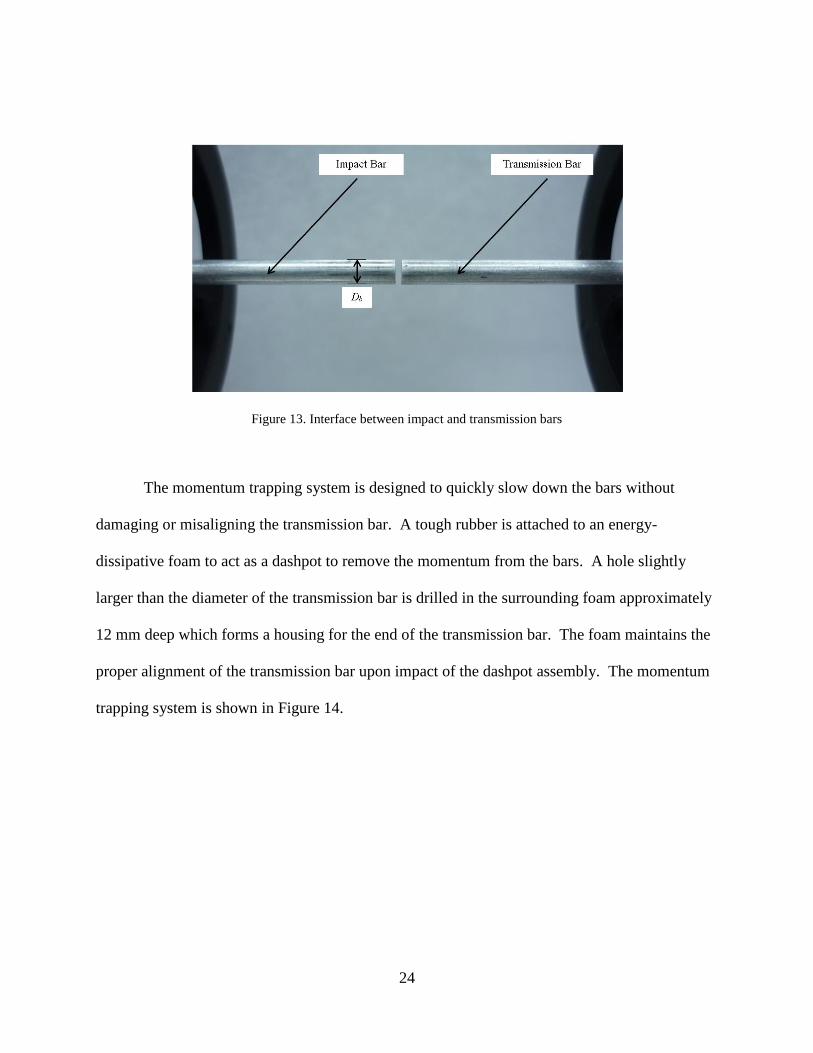
Figure 13. Interface between impact and transmission bars
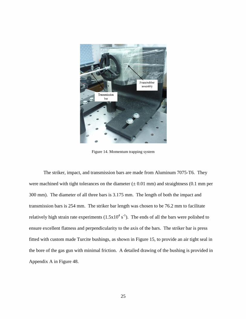
The momentum trapping system is designed to quickly slow down the bars without
damaging or misaligning the transmission bar. A tough rubber is attached to an energy-
dissipative foam to act as a dashpot to remove the momentum from the bars. A hole slightly
larger than the diameter of the transmission bar is drilled in the surrounding foam approximately
12 mm deep which forms a housing for the end of the transmission bar. The foam maintains the
proper alignment of the transmission bar upon impact of the dashpot assembly. The momentum
trapping system is shown in Figure 14.
25
Figure 14. Momentum trapping system
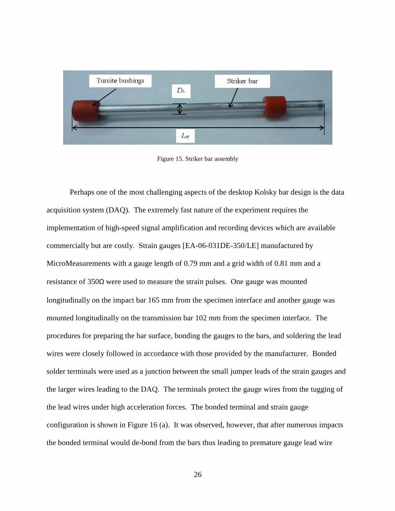
The striker, impact, and transmission bars are made from Aluminum 7075-T6. They
were machined with tight tolerances on the diameter (± 0.01 mm) and straightness (0.1 mm per
300 mm). The diameter of all three bars is 3.175 mm. The length of both the impact and
transmission bars is 254 mm. The striker bar length was chosen to be 76.2 mm to facilitate
relatively high strain rate experiments (1.5x10⁴ s
-1). The ends of all the bars were polished to
ensure excellent flatness and perpendicularity to the axis of the bars. The striker bar is press
fitted with custom made Turcite bushings, as shown in Figure 15, to provide an air tight seal in
the bore of the gas gun with minimal friction. A detailed drawing of the bushing is provided in
Appendix A in Figure 48.
26
Figure 15. Striker bar assembly
Perhaps one of the most challenging aspects of the desktop Kolsky bar design is the data
acquisition system (DAQ). The extremely fast nature of the experiment requires the
implementation of high-speed signal amplification and recording devices which are available
commercially but are costly. Strain gauges [EA-06-031DE-350/LE] manufactured by
MicroMeasurements with a gauge length of 0.79 mm and a grid width of 0.81 mm and a
resistance of 350Ω were used to measure the strain pulses. One gauge was mounted
longitudinally on the impact bar 165 mm from the specimen interface and another gauge was
mounted longitudinally on the transmission bar 102 mm from the specimen interface. The
procedures for preparing the bar surface, bonding the gauges to the bars, and soldering the lead
wires were closely followed in accordance with those provided by the manufacturer. Bonded
solder terminals were used as a junction between the small jumper leads of the strain gauges and
the larger wires leading to the DAQ. The terminals protect the gauge wires from the tugging of
the lead wires under high acceleration forces. The bonded terminal and strain gauge
configuration is shown in Figure 16 (a). It was observed, however, that after numerous impacts
the bonded terminal would de-bond from the bars thus leading to premature gauge lead wire

27
failure. The bonded terminal joint and lead wires were reinforced with a thin strip of electrical
tape as shown in Figure 16 (b). The tape effectively protected the lead wires and added strength
to the bonded terminal joint preventing gauge failure.
Figure 16. Bonded terminal and strain gauge configuration (a) and reinforced gauge (b)
Each of the gauges is connected to a quarter Wheatstone bridge completion module
(BCM-1 Omega) employing the three lead wire configuration to increase gauge sensitivity and
provide automatic temperature compensation. To amplify the signal from the Wheatstone
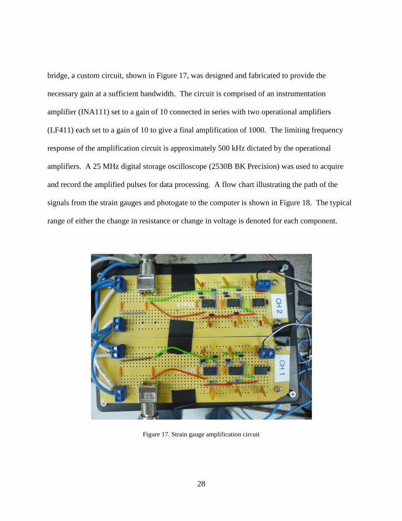
28
bridge, a custom circuit, shown in Figure 17, was designed and fabricated to provide the
necessary gain at a sufficient bandwidth. The circuit is comprised of an instrumentation
amplifier (INA111) set to a gain of 10 connected in series with two operational amplifiers
(LF411) each set to a gain of 10 to give a final amplification of 1000. The limiting frequency
response of the amplification circuit is approximately 500 kHz dictated by the operational
amplifiers. A 25 MHz digital storage oscilloscope (2530B BK Precision) was used to acquire
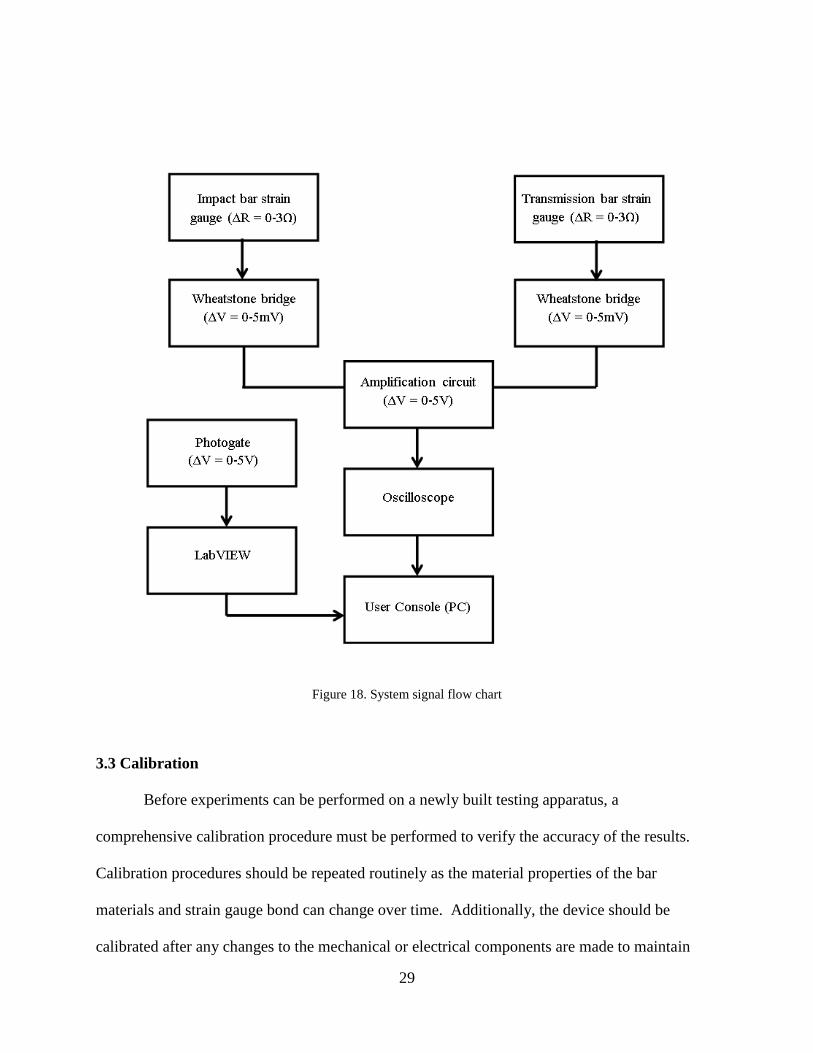
and record the amplified pulses for data processing. A flow chart illustrating the path of the
signals from the strain gauges and photogate to the computer is shown in Figure 18. The typical
range of either the change in resistance or change in voltage is denoted for each component.
Figure 17. Strain gauge amplification circuit
29
Figure 18. System signal flow chart
3.3 Calibration
Before experiments can be performed on a newly built testing apparatus, a
comprehensive calibration procedure must be performed to verify the accuracy of the results.
Calibration procedures should be repeated routinely as the material properties of the bar
materials and strain gauge bond can change over time. Additionally, the device should be
calibrated after any changes to the mechanical or electrical components are made to maintain
30
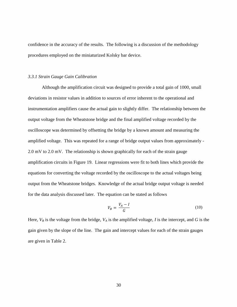
confidence in the accuracy of the results. The following is a discussion of the methodology
procedures employed on the miniaturized Kolsky bar device.
3.3.1 Strain Gauge Gain Calibration
Although the amplification circuit was designed to provide a total gain of 1000, small
deviations in resistor values in addition to sources of error inherent to the operational and
instrumentation amplifiers cause the actual gain to slightly differ. The relationship between the
output voltage from the Wheatstone bridge and the final amplified voltage recorded by the
oscilloscope was determined by offsetting the bridge by a known amount and measuring the
amplified voltage. This was repeated for a range of bridge output values from approximately -
2.0 mV to 2.0 mV. The relationship is shown graphically for each of the strain gauge
amplification circuits in Figure 19. Linear regressions were fit to both lines which provide the
equations for converting the voltage recorded by the oscilloscope to the actual voltages being
output from the Wheatstone bridges. Knowledge of the actual bridge output voltage is needed
for the data analysis discussed later. The equation can be stated as follows
(10)
Here, VB is the voltage from the bridge, VA is the amplified voltage, I is the intercept, and G is the
gain given by the slope of the line. The gain and intercept values for each of the strain gauges
are given in Table 2.

31
Figure 19. Strain gauge gain calibration plot
Table 2. Strain gauge gain calibration values
Strain Gauge Gain Intercept (mV)
Impact Bar 1208.5 78.5
Transmission Bar 1203.8 -174.2
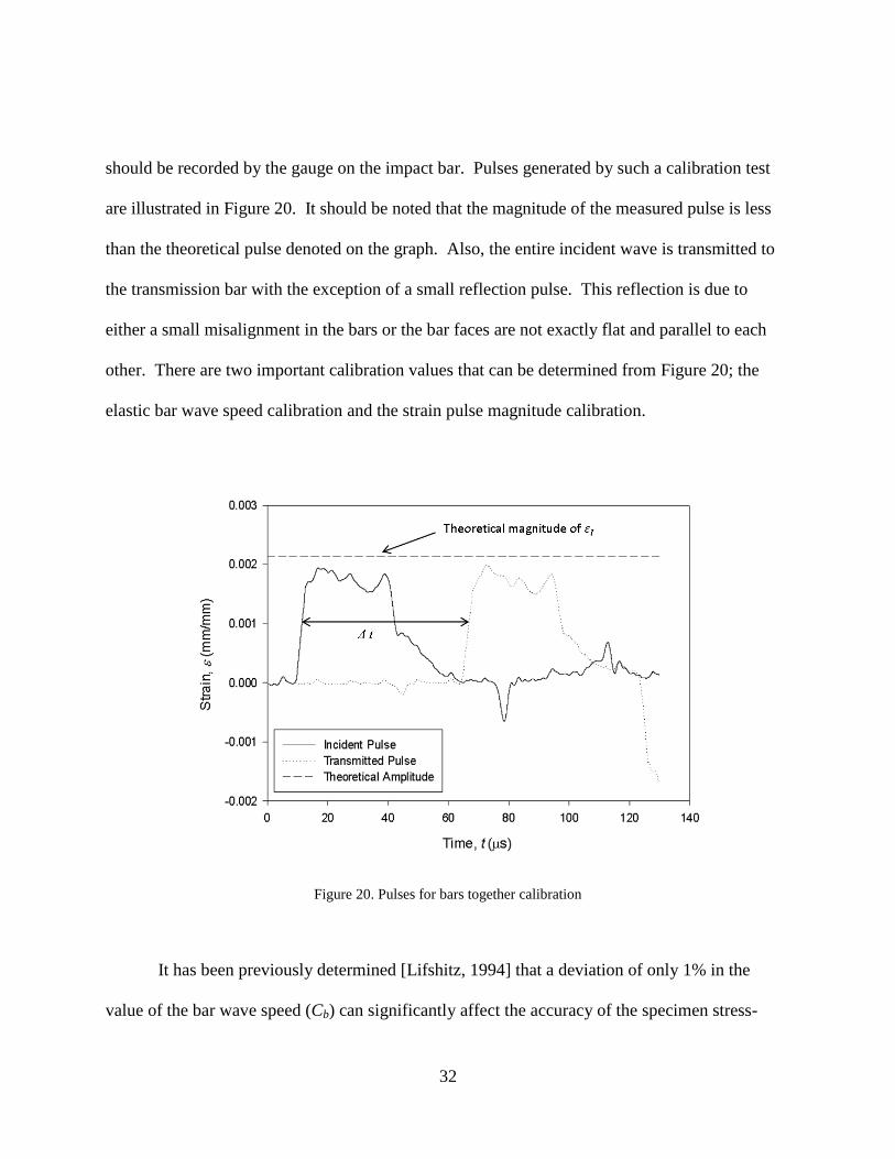
3.3.2 Strain Pulse Calibration
The calibration method discussed here compares the magnitude of the strain pulse
measured by the gauges to the theoretical magnitude for the case where the impact and
transmission bars are initially in direct contact. This is termed a “bars together” calibration. For
such a condition, the magnitude ( ) and period (T) of the incident pulse can be analytically
determined by Eqs. (2) and (3), respectively. If the bars are properly aligned and the bar surfaces
are sufficiently flat, the entire pulse should transfer into the transmission bar and no reflection
32
should be recorded by the gauge on the impact bar. Pulses generated by such a calibration test
are illustrated in Figure 20. It should be noted that the magnitude of the measured pulse is less
than the theoretical pulse denoted on the graph. Also, the entire incident wave is transmitted to
the transmission bar with the exception of a small reflection pulse. This reflection is due to
either a small misalignment in the bars or the bar faces are not exactly flat and parallel to each
other. There are two important calibration values that can be determined from Figure 20; the
elastic bar wave speed calibration and the strain pulse magnitude calibration.
Figure 20. Pulses for bars together calibration
It has been previously determined [Lifshitz, 1994] that a deviation of only 1% in the
value of the bar wave speed (Cb) can significantly affect the accuracy of the specimen stress-

33
strain plot determined from Kolsky bar experiments. Therefore, instead of using handbook
values for the elastic modulus and density of the bars to calculate the wave speed, the wave
speed was determined by measuring the time it takes for the pulses to travel from the gauge on
the impact bar to the gauge on the transmission bar. Specifically, the time between the two
pulses at a strain value of 0.001, as denoted in Figure 20 as Δt, was measured for 20 experiments
with the bars initially in direct contact. The travel time was determined to be 55.2 μs. The
distance between the two gauges was measured at 273 mm. Thus, the calibrated value of elastic
wave speed for the aluminum bars used in the miniaturized Kolsky bar apparatus is 4943 m/s.
This value is approximately 2% from the theoretical wave speed value of 5051 m/s calculated
from the handbook values of aluminum 7075-T6.
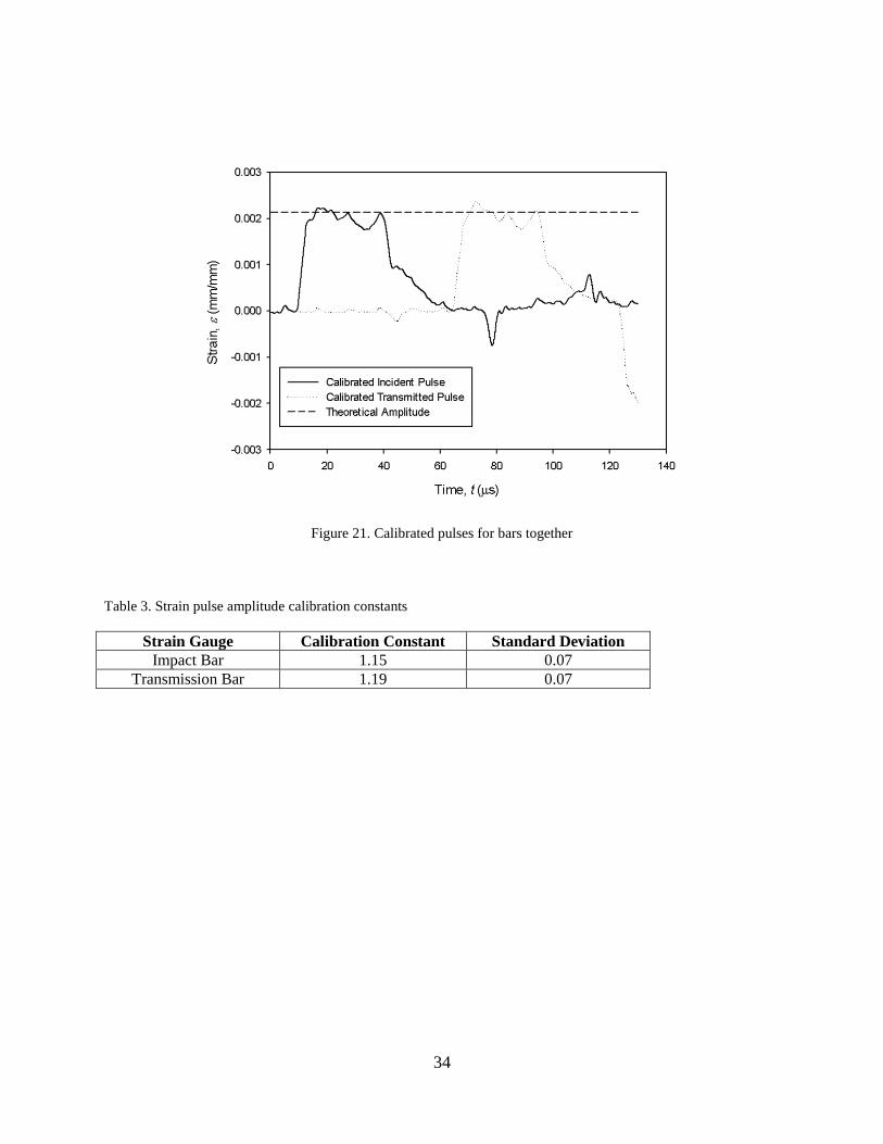
The calibration of the strain pulse magnitude is also critical for accurate specimen stress-
strain results. The difference between the recorded and theoretical pulses arises from a number
of errors characteristic of Kolsky bar experiments. Examples include the deviation from the
assumed one-dimensional wave propagation behavior and the effects of the strain gauge bond.
To compensate for these errors, the magnitude of the theoretical pulse based on the striker length
and calibrated wave speed is compared to the recorded pulse. This magnitude is denoted in
Figure 20 as a horizontal line. For each of the 20 “bars together” experiments, the ratio between
the theoretical pulse amplitude and the measured amplitudes for each strain gauge were
calculated. Even over the wide range of striker velocities at which the experiments were
conducted (9-25 m/s), the calibration values were nearly constant. The average and standard
deviations for the strain pulse amplitude calibration constants are provided in Table 3. The
pulses from Figure 20 are shown again in Figure 21 after the calibration correction was applied.
34
Figure 21. Calibrated pulses for bars together
Table 3. Strain pulse amplitude calibration constants
Strain Gauge Calibration Constant Standard Deviation
Impact Bar 1.15 0.07
Transmission Bar 1.19 0.07
35
4. EXPERIMENTAL SETUP
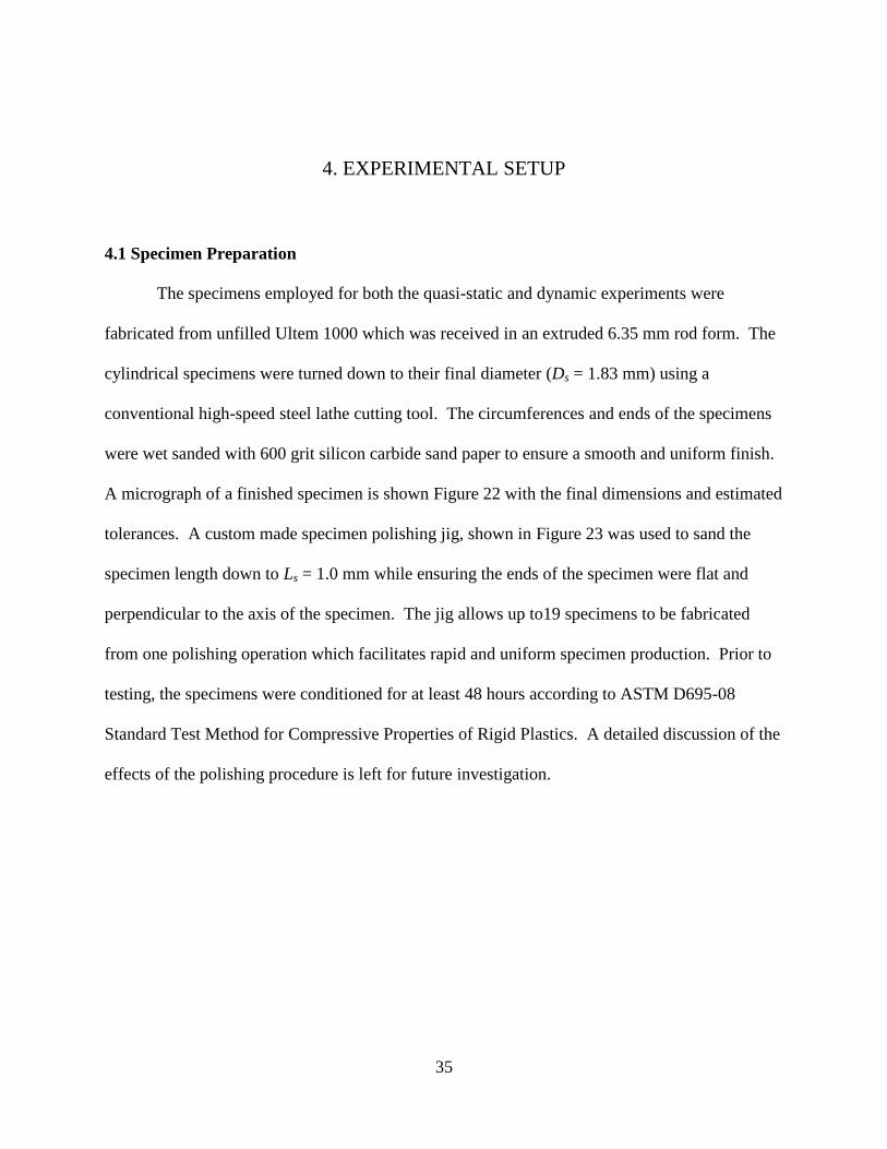
4.1 Specimen Preparation
The specimens employed for both the quasi-static and dynamic experiments were
fabricated from unfilled Ultem 1000 which was received in an extruded 6.35 mm rod form. The
cylindrical specimens were turned down to their final diameter (Ds = 1.83 mm) using a
conventional high-speed steel lathe cutting tool. The circumferences and ends of the specimens
were wet sanded with 600 grit silicon carbide sand paper to ensure a smooth and uniform finish.
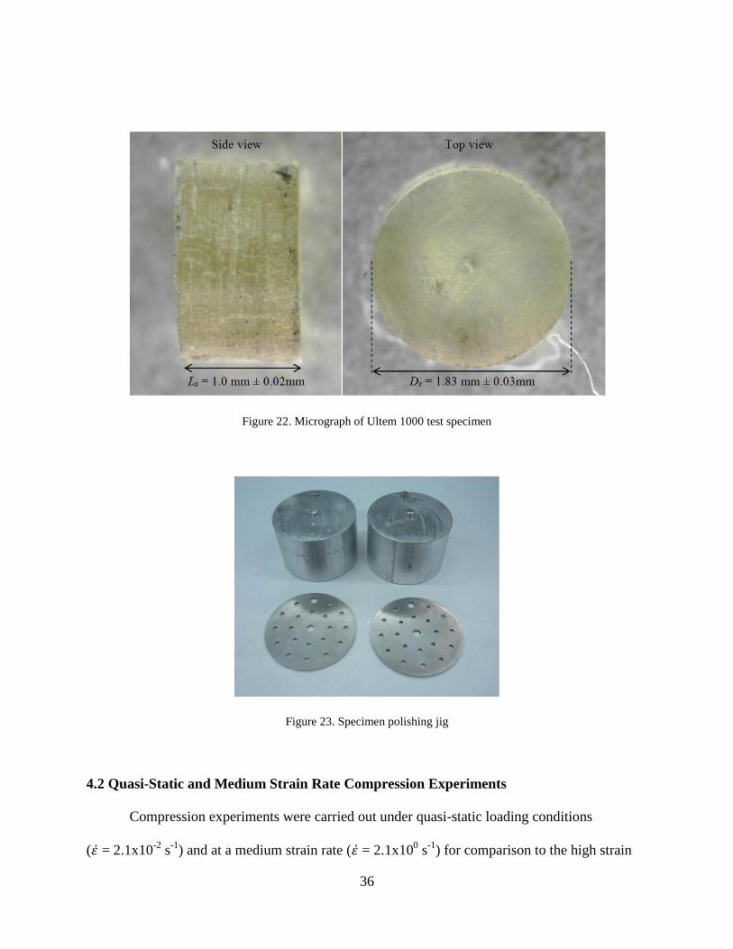
A micrograph of a finished specimen is shown Figure 22 with the final dimensions and estimated
tolerances. A custom made specimen polishing jig, shown in Figure 23 was used to sand the
specimen length down to Ls = 1.0 mm while ensuring the ends of the specimen were flat and
perpendicular to the axis of the specimen. The jig allows up to19 specimens to be fabricated
from one polishing operation which facilitates rapid and uniform specimen production. Prior to
testing, the specimens were conditioned for at least 48 hours according to ASTM D695-08
Standard Test Method for Compressive Properties of Rigid Plastics. A detailed discussion of the
effects of the polishing procedure is left for future investigation.
36
Figure 22. Micrograph of Ultem 1000 test specimen
Figure 23. Specimen polishing jig
4.2 Quasi-Static and Medium Strain Rate Compression Experiments
Compression experiments were carried out under quasi-static loading conditions
( = 2.1x10⁻²
s-1
) and at a medium strain rate ( = 2.1x100 s
-1) for comparison to the high strain

37
rate mechanical behavior of Ultem 1000. The compression experiments were conducted on an
electromechanical MTS Insight 5kN universal testing frame and an MTS 634.11E-25 axial
extensometer was used to record the deflection of the specimens. As shown in Figure 24, the
extensometer is contacting the surface of the compression platens instead of the specimen
because the length of the specimen was below the minimum measurable length of the
extensometer. Since the stiffness of the platens is much greater than that of the Ultem
specimens, it was assumed that any deflection measured by the extensometer was due to the
specimen only. A molybdenum disulfide based lubricant was used to reduce the friction between
the platen and specimen surfaces.
Figure 24. Test configuration used in quasi-static testing

38
4.3 Kolsky Bar Experiments
To characterize the high strain rate behavior of Ultem 1000, Kolsky bar experiments were
conducted at a range of strain rates from 8.7x10³ to 1.5x10
4 s
-1. A minimum of three
experiments were performed at each strain rate. The velocity of the striker bar can be used to
estimate the strain rate of an experiment, but the actual strain rate, which is averaged over the
stable duration of the test, can only be determined after processing the data and employing Eq.
(4).
Before an experiment is performed on the miniaturized Kolsky bar apparatus, power to
the Wheatstone bridges and amplification circuits is supplied for at least 20 minutes to allow the
circuitry to warm up and stabilize. The excitation voltage powering the two Wheatstone bridges
is 3.3 V which is the optimal voltage based on the strain gauge size, type, and bar. The length
and diameter of each specimen is measured just prior to the experiment using a micrometer with
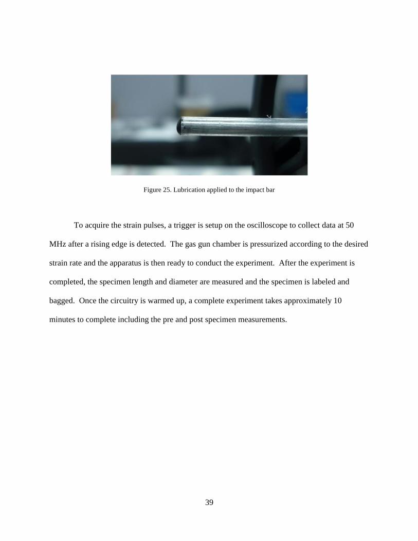
a resolution of 0.0254 mm. The same molybdenum disulfide based lubricant used in the quasi-
static experiments is applied to the ends of both the impact and transmission bars as shown in
Figure 25. The specimen is carefully placed in between the two bars as they are brought together
and the excess lubrication is wiped away. Once the specimen is centered such that it is coaxial
with the bars, a clear box is placed around the specimen designed to contain the specimen during
the experiment so that it can be recovered. A properly aligned specimen about to be tested is
shown in Figure 26.
39
Figure 25. Lubrication applied to the impact bar
To acquire the strain pulses, a trigger is setup on the oscilloscope to collect data at 50
MHz after a rising edge is detected. The gas gun chamber is pressurized according to the desired
strain rate and the apparatus is then ready to conduct the experiment. After the experiment is
completed, the specimen length and diameter are measured and the specimen is labeled and
bagged. Once the circuitry is warmed up, a complete experiment takes approximately 10
minutes to complete including the pre and post specimen measurements.

40
Figure 26. Specimen in Kolsky bar experiment

41
5. EXPERIMENTAL RESULTS
5.1 Quasi-Static and Medium Strain Rate Compression Results
The stress-strain curves discussed in the ensuing sections are in terms of the true rather
than the engineering values of stress and strain. The conversion from engineering stress ( )
and engineering strain (e ) to true stress (σ) and true strain (ε) is given by
(11)
(12)
The above equations are only valid for the case of constant volume deformation which was
verified for both the quasi-static and Kolsky experiments by measuring the specimen dimensions
before and after each test. Stress-strain curves representative of the average response for both
the quasi-static and medium strain rate compression experiments are shown in Figure 27. The
curves exhibit a four stage response (linear elastic, nonlinear elastic, strain softening, strain
hardening) typical of amorphous polymers. The average yield stress was found to be 166 MPa
and 193 MPa at strain rates of 2.1x10⁻²
and 2.1x100, respectively.

42
Figure 27. Quasi-static stress strain curves
5.2 Kolsky Bar Results
5.2.1 Data Analysis
Ideally, the Kolsky bar apparatus will provide the stress-strain curve for the specimen
throughout the entire loading duration, which is governed by Eq. (3). Also, under ideal
conditions, the strain rate would be constant during the entire loading phase. From these stress-
strain curves, a relationship between strain rate and the mechanical properties such as elastic
modulus, yield strength, ultimate strength, and the hardening/softening behavior can be
determined. However, due to some of the limitations inherent to the Kolsky bar apparatus, the
strain rate is not exactly constant throughout the test and there is a finite time during which the
specimen is not in stress equilibrium. During this time, known as the “ring-up period,” Eq. (4)

43
and Eq. (5) are not valid. The ring-up period duration, τ, is the time it takes for π reverberations
to traverse through the specimen [Davies and Hunter] and is expressed
(13)
where Ls is the initial length of the specimen and Cs is the elastic wave speed of the specimen.
Therefore, the stress-strain response of the material before τ seconds cannot be considered valid.
Often times this means that the elastic portion of the stress strain curve cannot be accurately
determined. Methods have been developed to decrease the ring up period and to increase the
duration at which the strain rate is constant through a technique referred to as “pulse shaping.”
These techniques were not employed in the current Kolsky bar apparatus, but are saved for future
work and are discussed in Chapter 6
To illustrate how the pulses recorded during a Kolsky bar experiment are analyzed and
how they are checked for validity, an example is provided here detailing the steps taken to fully
process the experimental data. The data analysis procedure includes data smoothing, pulse
synchronization, and algebraic manipulation of the pulses. A program was developed in
MATLAB (see Appendix C) to automatically perform the smoothing and algebraic operations.
Determining the starting and ending points of the incident, transmitted, and reflected pulses was
done manually, which if done incorrectly introduces error in the stress-strain curve [Chen, 2011].
The pulses that are acquired from the oscilloscope are in terms of an amplified voltage and are
slightly offset from zero due to the Wheatstone bridges being initially unbalanced. Before the
pulses can be converted from voltage to strain, the amplified voltage is converted into the actual
bridge output voltage by employing the strain gauge gain calibration equation discussed in
Section 3.3.1. The voltage now is on the order of a few millivolts instead of on the order of volts

44
which was recorded by the oscilloscope. The baselines of these pulses are then shifted to zero by
taking the average of the output voltage for 20 μs before the impact is recorded and subtracting
this offset value from the magnitude of the pulses. The voltages are then converted into strain
using the one-quarter Wheatstone bridge equation below
(14)
where ΔV is the change in output bridge voltage, Gf is the gauge factor for the gauges used and
VE is the bridge excitation voltage. The pulses, now in terms of strain, are multiplied by the
strain amplitude calibration constants discussed in Section 3.3.2. Finally, the strain pulses are
smoothed using a local weighted regression algorithm. The data analysis code provided in
Appendix C performs all of these operations automatically for each experimental data set. The
example experiment was conducted on an Ultem specimen with dimensions Ls = 1.039 mm and
Ds = 1.778 mm and with a striker velocity of 23.8 m/s. Therefore, according to Eq. (3), the pulse
width should be approximately 31 μs. The processed pulses for this example case are illustrated
in Figure 28.

45
Figure 28. Post-processed strain pulses from example Kolsky bar experiment
The next procedure is to synchronize the three pulses by first determining their start and
end points and then eliminate the time variable between them as shown in Figure 29. To check
the validity of the stress equilibrium assumption, the incident and reflected pulses are added
together and compared to the transmitted pulses, as shown in Figure 30. Only for times at which
the addition of the incident and reflected pulses is sufficiently close to the transmitted pulse is the
specimen in stress equilibrium. The percent difference between the transmitted pulse and the
addition of the incident and reflected pulses are shown graphically in Figure 31. Although the
ring-up duration given by Eq. (13) for Ultem is approximately 2 μs, it can be seen from Figure
31 that for the miniaturized Kolsky bar apparatus discussed here the time is approximately 4μs.

46
Figure 29. Synchronized strain pulses
Figure 30. Stress equilibrium comparison graph

47
Figure 31. Stress equilibrium verification graph
The other condition that must be checked to determine the validity of the test results is
the duration of the test at which the specimen is under a constant strain rate. The strain rate as a
function of time is given by Eq. (4) and is shown graphically for the example case in Figure 32.
Clearly, from Figure 32 it is seen that the strain rate is not constant throughout the duration of the
test, but an average strain rate after 4 μs is used as the strain rate for the experiment and is
calculated to be approximately 14470 s-1
for the present example. The accumulated strain in the
specimen as a function of time, shown in Figure 33 is found by integrating Eq. (4) at each time
increment and adding the individual strain increments. The value of strain at 4 μs is
approximately 2%. Hence, the stress response corresponding to strains less than 2% cannot be
accurately determined for this particular experiment due to the ring-up period. When the stress

48
as a function of time, calculated from Eq. (5) is superimposed with the strain as a function of
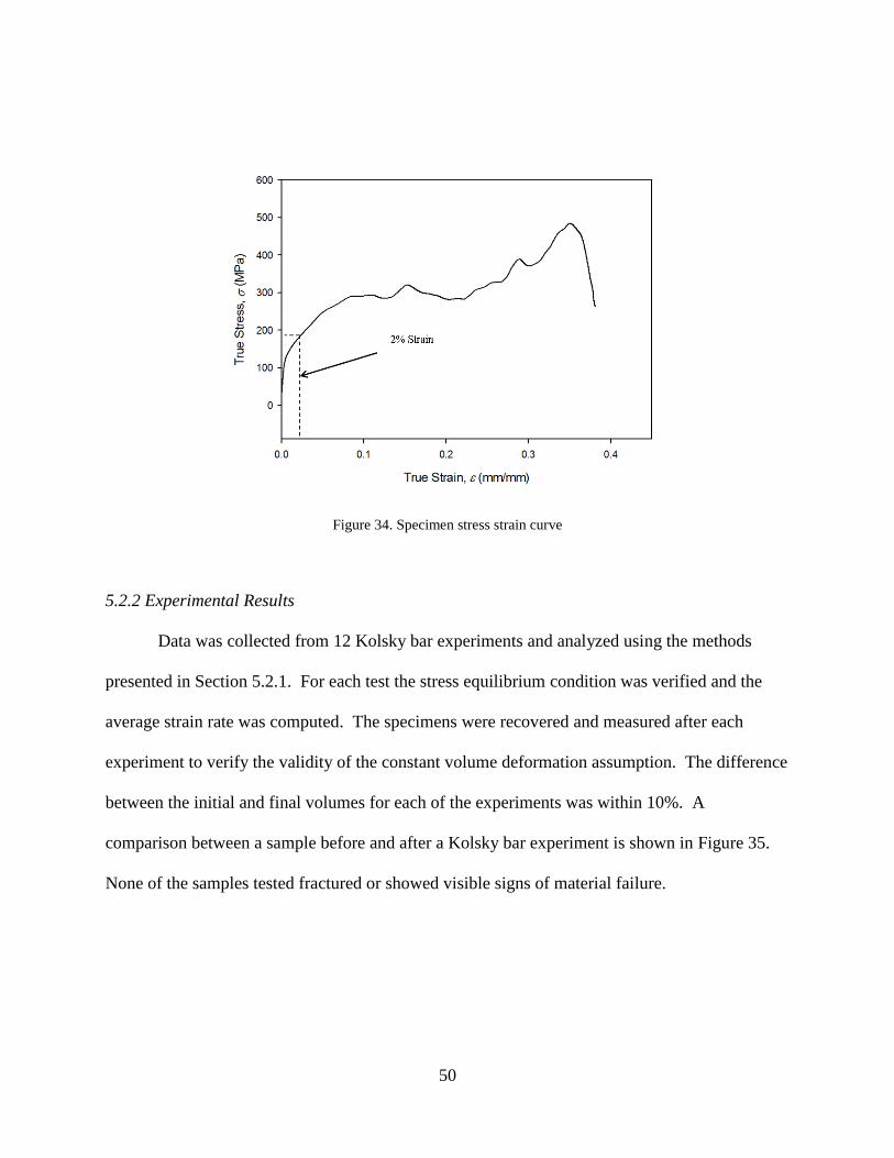
time, the engineering stress-strain curve is produced as shown in Figure 34. Again, a line is
shown on the graph denoting the point before which the data cannot be validated. From Figure
34 the typical mechanical material properties can be estimated such as yield stress, ultimate
stress, and the hardening/softening behavior.
Figure 32. Strain rate versus time
In summary, the data analysis procedure consists of processing the raw voltage pulse data
recorded from the oscilloscope by smoothing and scaling it according to the calibration constants
discussed in Chapter 3. Next the voltage is converted into strain through Eq. (14) and the
incident, reflected, and transmitted pulses are synchronized from which the strain rate and stress
as functions of time are calculated. The portion of the data that can be validated is determined
by investigating the stress equilibrium and strain rate characteristics of the data. Finally, the true

49
stress-strain response is created from which the mechanical behavior of the specimen at that
particular strain rate can be determined. This process is repeated for experiments at a range of
strain rates to characterize the relationship between the mechanical behavior of the specimen
material and strain rate.
Figure 33. Specimen strain versus time
50
Figure 34. Specimen stress strain curve
5.2.2 Experimental Results
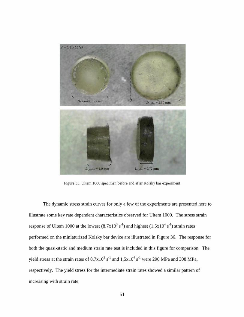
Data was collected from 12 Kolsky bar experiments and analyzed using the methods
presented in Section 5.2.1. For each test the stress equilibrium condition was verified and the
average strain rate was computed. The specimens were recovered and measured after each
experiment to verify the validity of the constant volume deformation assumption. The difference
between the initial and final volumes for each of the experiments was within 10%. A
comparison between a sample before and after a Kolsky bar experiment is shown in Figure 35.
None of the samples tested fractured or showed visible signs of material failure.
51
Figure 35. Ultem 1000 specimen before and after Kolsky bar experiment
The dynamic stress strain curves for only a few of the experiments are presented here to
illustrate some key rate dependent characteristics observed for Ultem 1000. The stress strain
response of Ultem 1000 at the lowest (8.7x10³ s
-1) and highest (1.5x10
4 s
-1) strain rates
performed on the miniaturized Kolsky bar device are illustrated in Figure 36. The response for
both the quasi-static and medium strain rate test is included in this figure for comparison. The
yield stress at the strain rates of 8.7x10³ s
-1 and 1.5x10
4 s
-1 were 290 MPa and 308 MPa,
respectively. The yield stress for the intermediate strain rates showed a similar pattern of
increasing with strain rate.

52
Figure 36. Stress-strain curves of Ultem 1000 at various strain rates
To illustrate the relationship between the strain rate and yield stress of Ultem 1000, the
yield stress for a wide range of strain rates is plotted against the corresponding strain rate as
shown in Figure 37. Clearly, the yield stress of Ultem 1000 exhibits a distinct bilinear
dependence on log( ). It appears that the transition occurs at approximately 1.2x10³ s
-1.
53
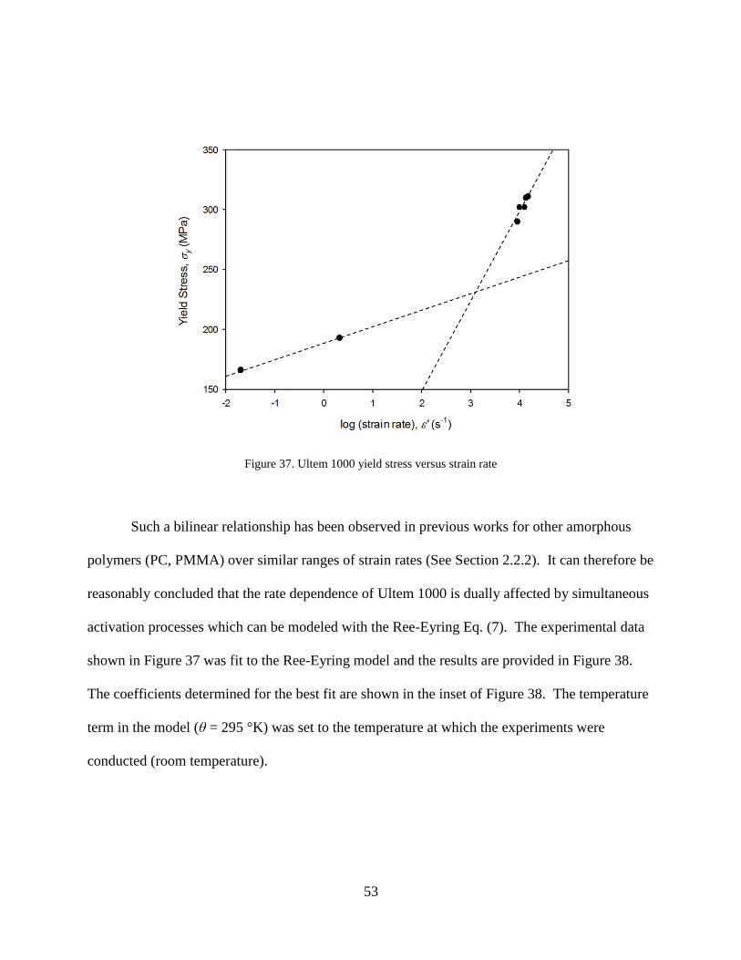
Figure 37. Ultem 1000 yield stress versus strain rate
Such a bilinear relationship has been observed in previous works for other amorphous
polymers (PC, PMMA) over similar ranges of strain rates (See Section 2.2.2). It can therefore be
reasonably concluded that the rate dependence of Ultem 1000 is dually affected by simultaneous
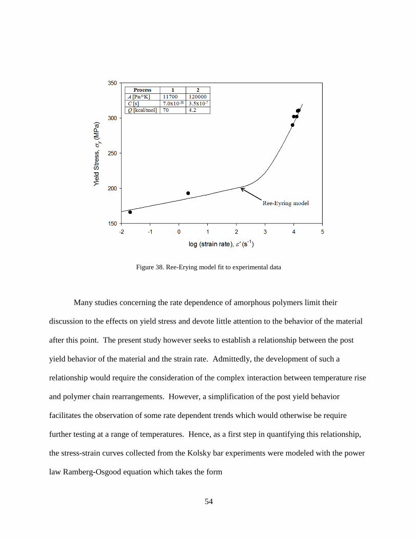
activation processes which can be modeled with the Ree-Eyring Eq. (7). The experimental data
shown in Figure 37 was fit to the Ree-Eyring model and the results are provided in Figure 38.
The coefficients determined for the best fit are shown in the inset of Figure 38. The temperature
term in the model (θ = 295 °K) was set to the temperature at which the experiments were
conducted (room temperature).
54
Figure 38. Ree-Erying model fit to experimental data
Many studies concerning the rate dependence of amorphous polymers limit their
discussion to the effects on yield stress and devote little attention to the behavior of the material
after this point. The present study however seeks to establish a relationship between the post
yield behavior of the material and the strain rate. Admittedly, the development of such a
relationship would require the consideration of the complex interaction between temperature rise
and polymer chain rearrangements. However, a simplification of the post yield behavior
facilitates the observation of some rate dependent trends which would otherwise be require
further testing at a range of temperatures. Hence, as a first step in quantifying this relationship,
the stress-strain curves collected from the Kolsky bar experiments were modeled with the power
law Ramberg-Osgood equation which takes the form

55
(15)
where εp is the plastic strain and K and n are fitting parameters that describe the yield point and
hardening behavior, respectively. A comparison between the experimental stress-strain data and
the model is illustrated in Figure 39. The plastic portion of the strain (εp) is separated from the
total strain (ε) by subtracting the elastic strain, i.e.,
(16)
Here, E is the slope of the initial linear portion of the stress strain response. It is appropriate to
limit the scope of the mathematical modeling to only the plastic strains as defined by Eq. (16)
since the response in the elastic strain range cannot be accurately determined for the Kolsky bar
experiments discussed here (See Section 5.2.1).
Figure 39. Ramberg-Osgood model fit of experimental data

56
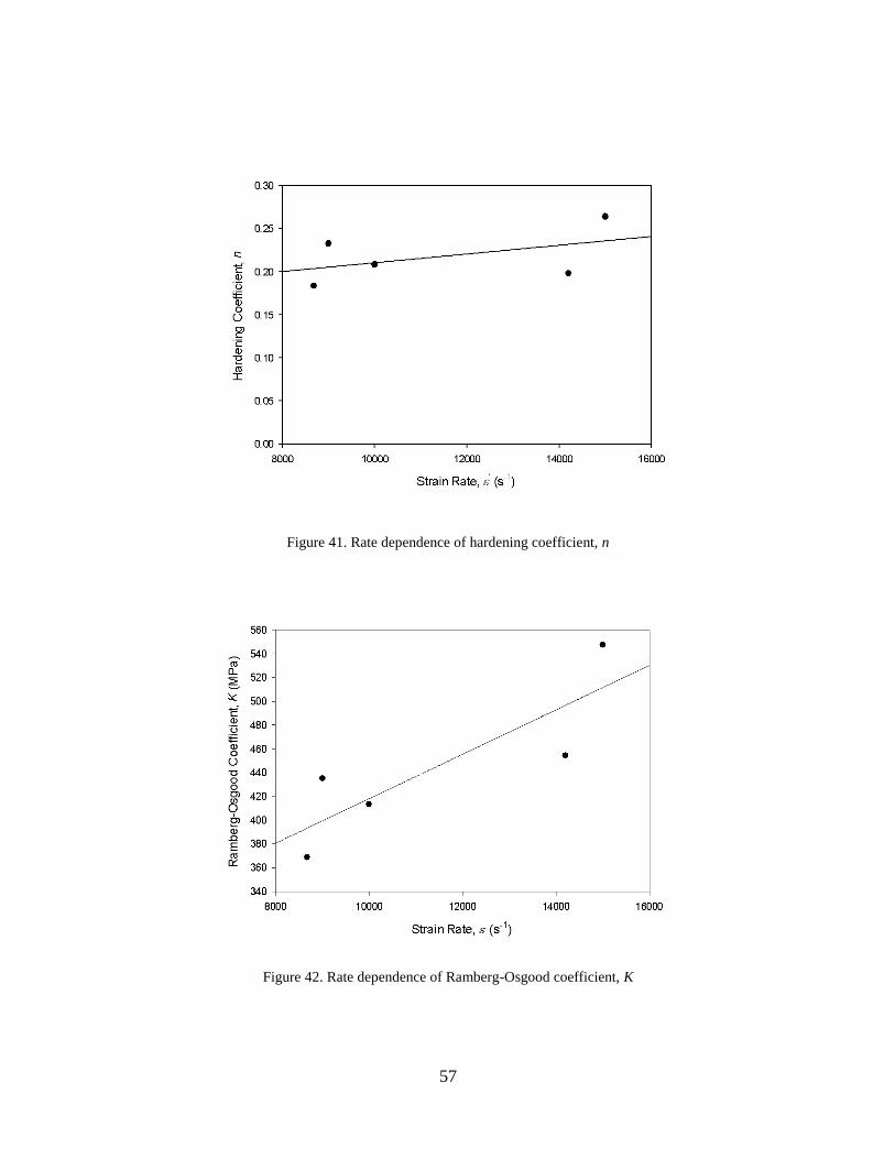
The stress-strain curves for various strain rates between 8.7x10³ s
-1 and 1.5x10
4 s
-1 were
fit to Eq. (15) and the results are provided in Figure 40. An observation readily made from
Figure 40 is that the slope of the hardening portion of each of the curves is nearly a constant for
each of the strain rates. This relationship can be easily seen by plotting the hardening
coefficient, n, against the strain rate and observing a nearly linear correlation as is the case in
Figure 41. The rate dependence of the Ramberg-Osgood coefficient K was found to increase
linearly with strain rate, as is shown in Figure 42.
Figure 40. Ramberg-Osgood model for various strain rates
57
Figure 41. Rate dependence of hardening coefficient, n
Figure 42. Rate dependence of Ramberg-Osgood coefficient, K

58
6. DISCUSSION
Overall, the experimental results for both the quasi-static and high strain rate tests were
consistent with trends observed previously for other amorphous polymers. This fact provides a
level of confidence in the operation of the Kolsky bar device and in the data analysis techniques.
The quasi-static stress strain behavior of Ultem 1000 exhibits the typical response for an
amorphous polymer which has been well defined in terms of polymer chain sliding and
rearranging. At this low strain rate, the effects of temperature rises due to plastic deformation
can be ignored.
Regarding the high strain rate experiments, perhaps the most noticeable trend is the
bilinear relationship between the yield stress and the log( ). For Ultem 1000, the transition
between the two linear regions is approximately 103 s
-1. This transition point is similar to that of
PC and PMMA determined by Walley and others [Walley, 1991]. Determining a more precise
value for this transition point would require additional experiments in the range of 101 to 10
3 s
-1
which are out of the operating range of both standard electromechanical test frames and Kolsky
bar devices. Determining the cause of this transition is of considerable interest, especially if a
molecular based constitutive model is to be developed. Past investigators have explained this
bilinear relationship in terms of two activation processes concurrently taking place and the
second process becoming dominant after the transition point. In order to fully understand the
mechanisms causing this transition, the effects of local temperature rises must be considered.
The effect of temperature on the stress-strain response can be investigated in two ways. One
method would be to measure any thermal changes during an experiment and try to correlate this
to an activation process. A secondary method to investigate thermal effects would be to
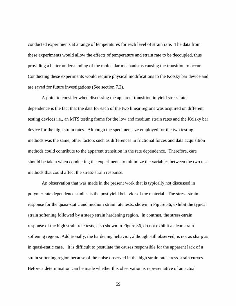
59
conducted experiments at a range of temperatures for each level of strain rate. The data from
these experiments would allow the effects of temperature and strain rate to be decoupled, thus
providing a better understanding of the molecular mechanisms causing the transition to occur.
Conducting these experiments would require physical modifications to the Kolsky bar device and
are saved for future investigations (See section 7.2).
A point to consider when discussing the apparent transition in yield stress rate
dependence is the fact that the data for each of the two linear regions was acquired on different
testing devices i.e., an MTS testing frame for the low and medium strain rates and the Kolsky bar
device for the high strain rates. Although the specimen size employed for the two testing
methods was the same, other factors such as differences in frictional forces and data acquisition
methods could contribute to the apparent transition in the rate dependence. Therefore, care
should be taken when conducting the experiments to minimize the variables between the two test
methods that could affect the stress-strain response.
An observation that was made in the present work that is typically not discussed in
polymer rate dependence studies is the post yield behavior of the material. The stress-strain
response for the quasi-static and medium strain rate tests, shown in Figure 36, exhibit the typical
strain softening followed by a steep strain hardening region. In contrast, the stress-strain
response of the high strain rate tests, also shown in Figure 36, do not exhibit a clear strain
softening region. Additionally, the hardening behavior, although still observed, is not as sharp as
in quasi-static case. It is difficult to postulate the causes responsible for the apparent lack of a
strain softening region because of the noise observed in the high strain rate stress-strain curves.
Before a determination can be made whether this observation is representative of an actual

60
material response or a mere artifact of the available data, more experiments need to be conducted
with improvements to the Kolsky bar device to reduce noise. The differences in the hardening
behavior between the quasi-static and high strain rate experiments could be a result of
temperature rises in the material at the high strain rates. If it is assumed that the same molecular
mechanisms that cause strain hardening in quasi-static case (polymer chain realignment) are also
at work in the high strain rate cases, then the rise in temperature could have a softening effect on
the material in conjunction with the hardening process due to the polymer chain realignment.
This dual effect of polymer chain rearrangement with the introduction of heat generation could
explain why hardening is still observed, but to a lesser degree. However, to be sure, more
experiments should be conducted where the temperature rises are measured directly.
61
7. CONCLUSION AND FUTURE WORK
7.1 Conclusions
The achievements of the present work can be summarized into two categories: (1)
successful Kolsky bar apparatus design, construction, and operation and (2) material
characterization of Ultem 1000 over a wide range of strain rates. The provided methodologies
for designing and fabricating a miniaturized Kolsky bar device as well as the provided data
processing procedures and codes can serve as a guide to those seeking to build and employ these
devices. A method for fabricating the test specimens used for these experiments was presented
along with the engineering drawings for the custom polishing jig used. Additionally, the design
for an economical amplification circuit board capable of acquiring the signal pulses from Kolsky
bar experiments was provided.
The trends observed from the high strain rate testing of Ultem 1000 were consistent with
those for other amorphous polymers tested under similar conditions. Specifically, the
relationship between the yield stress and the log( ) was bilinear. This correlation was modeled
with the Ree-Eyring equation. Additionally, the differences between the post yield behavior of
the quasi-static and high strain rate experiments was observed and possible explanations were
provided.
7.2 Future Work
The Kolsky bar device in its present configuration is capable of testing a variety of
polymeric materials at room temperature from strain rates of approximately 103 s
-1 to 10
5 s
-1.
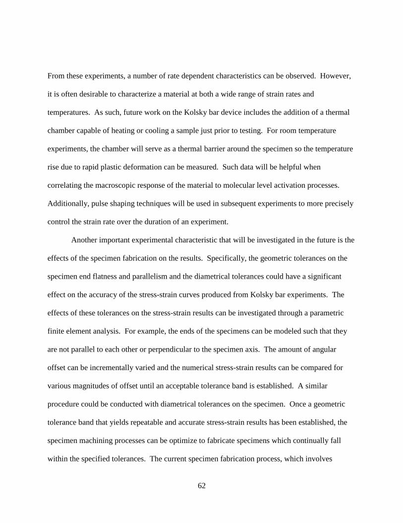
62
From these experiments, a number of rate dependent characteristics can be observed. However,
it is often desirable to characterize a material at both a wide range of strain rates and
temperatures. As such, future work on the Kolsky bar device includes the addition of a thermal
chamber capable of heating or cooling a sample just prior to testing. For room temperature
experiments, the chamber will serve as a thermal barrier around the specimen so the temperature
rise due to rapid plastic deformation can be measured. Such data will be helpful when
correlating the macroscopic response of the material to molecular level activation processes.
Additionally, pulse shaping techniques will be used in subsequent experiments to more precisely
control the strain rate over the duration of an experiment.
Another important experimental characteristic that will be investigated in the future is the
effects of the specimen fabrication on the results. Specifically, the geometric tolerances on the
specimen end flatness and parallelism and the diametrical tolerances could have a significant
effect on the accuracy of the stress-strain curves produced from Kolsky bar experiments. The
effects of these tolerances on the stress-strain results can be investigated through a parametric
finite element analysis. For example, the ends of the specimens can be modeled such that they
are not parallel to each other or perpendicular to the specimen axis. The amount of angular
offset can be incrementally varied and the numerical stress-strain results can be compared for
various magnitudes of offset until an acceptable tolerance band is established. A similar
procedure could be conducted with diametrical tolerances on the specimen. Once a geometric
tolerance band that yields repeatable and accurate stress-strain results has been established, the
specimen machining processes can be optimize to fabricate specimens which continually fall
within the specified tolerances. The current specimen fabrication process, which involves

63
considerable manual work, is time consuming and does not easily produce uniform specimens.
As such, an improved manufacturing process involving micro-milling is being developed which
is capable of fabricating specimens with a resolution of 50 micrometers. This fabrication process
will facilitate the rapid production of hundreds of nearly identical specimens with exceptional
geometric tolerances.
The end goal of many material characterization studies is the implementation of the
experimental results into a numerical simulation. This can be accomplished by either
determining the fitting constants for an existing constitutive model or by developing a novel
constitutive model. Future studies will attempt to fit the experimental data for Ultem 1000 into
existing constitutive models for amorphous polymers. Such a constitutive model can then be
employed in an explicit numerical simulation code, such as LS-DYNA, to verify the
experimental results as well as determine the response of Ultem 1000 under novel combinations
of temperature and load.

64
APPENDIX A: TEST HARDWARE

65
Figure 43. Launch tube drawing (dimensions in inches)

66
Figure 44. Launch tube alignment block drawing (dimensions in inches)

67
Figure 45. LH1 lens holder drawing (Thor Labs)
68
Figure 46. TR3 lens mount post drawing (Thor Labs)

69
Figure 47. PH2 post holder (Thor Labs)

70
Figure 48. Striker bar bushing drawing (dimensions are in inches)

71
APPENDIX B: STRIKER BAR VELOCITY LABVIEW VI
72
Figure 49. LabVIEW VI block diagram (a) and front panel (b)

73
APPENDIX C: DATA PROCESSING CODE

74
close all
clc
clear all
tic
% Define variables
file_name='ultem_data'; % File name
CH1_gain=1208.5; % Gain for CH1
CH2_gain=1203.8; % Gain for CH2
CH1_intcp=0.0785; % Gain intercept for CH1 (V)
CH2_intcp=-0.1742; % Gain intercept for CH2 (V)
gauge_factor=2.08; % Strain gauge factor
ex_volt=3.288; % Bridge excitation voltage (V)
Cb=4943; % Bar wave speed (m/s)
span=101; % Smoothing span value (must be odd)
run=1; % Refers to the sheet number in Excel
% Read record length and time increment
N=xlsread(file_name,run,'B1:B1');
inc=xlsread(file_name,run,'B2:B2');
for run=1:13 % Loop for all sheets
% Read time, incident pulse, and transmission pulse vectors
CH1=xlsread(file_name,run,'B14:B16397');
CH2=xlsread(file_name,run,'C14:C16397');
% Reduce magnitude of pulses using gain equation
CH1_gain=(CH1-CH1_intcp)/CH1_gain;
CH2_gain=(CH2-CH2_intcp)/CH2_gain;
% Determine pulse offset zeros
CH1_zero=mean(CH1_gain(1:500));
CH2_zero=mean(CH2_gain(1:500));
% Offset pulses to start at zero
CH1_adj=CH1_gain-CH1_zero;
CH2_adj=CH2_gain-CH2_zero;
% Convert pulses from voltage to strain
CH1_strain=(4*CH1_adj)/(gauge_factor*ex_volt);
CH2_strain=(4*CH2_adj)/(gauge_factor*ex_volt);

75
% Smooth data
CH1_smooth=smooth(CH1_strain,span,'rlowess');
CH2_smooth=smooth(CH2_strain,span,'rlowess');
% Build matrix of values to write back into excel workbook
output(:,1)=CH1_gain;
output(:,2)=CH2_gain;
output(:,3)=CH1_adj;
output(:,4)=CH2_adj;
output(:,5)=CH1_strain;
output(:,6)=CH2_strain;
output(:,7)=CH1_smooth;
output(:,8)=CH2_smooth;
% Write output matrix back into excel workbook
xlswrite(file_name,output,run,'D14:K16397');
end
toc

76
APPENDIX D: SPECIMENS AND TEST DATA

77
Table 4. Summary of Kolsky bar experimental data
Specimen # Average Strain Rate
s-1
Yield Stress
MPa
Total Strain
%
100 14277 289 32.5
101 12744 285 28.3
102 12787 302 28.7
103 12447 292 37.0
104 13235 293 35.6
107 8991 289 18.2
108 8677 308 12.6
109 10291 302 19.7
110 9441 309 20.3
111 13682 311 30.7
112 14509 311 25.2
113 14951 289 37.4
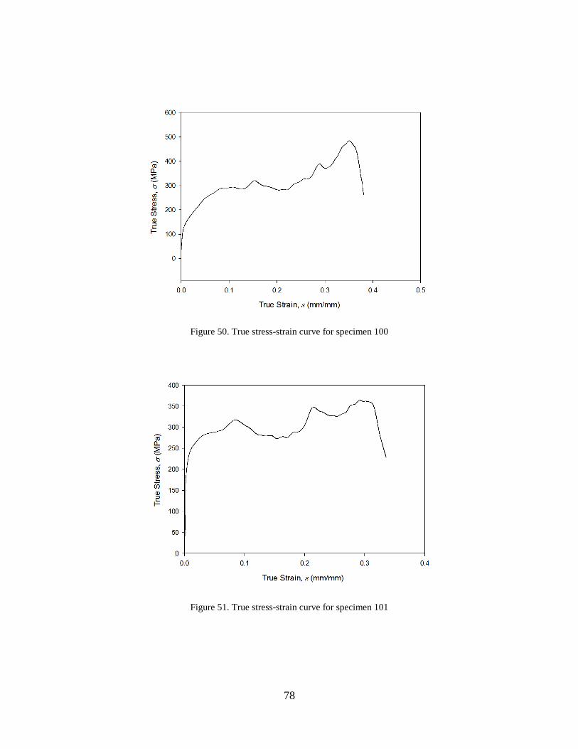
78
Figure 50. True stress-strain curve for specimen 100
Figure 51. True stress-strain curve for specimen 101
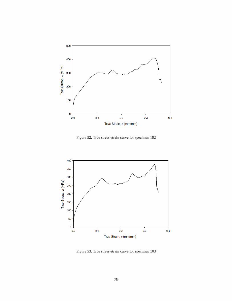
79
Figure 52. True stress-strain curve for specimen 102
Figure 53. True stress-strain curve for specimen 103

80
Figure 54. True stress-strain curve for specimen 104
Figure 55. True stress-strain curve for specimen 107
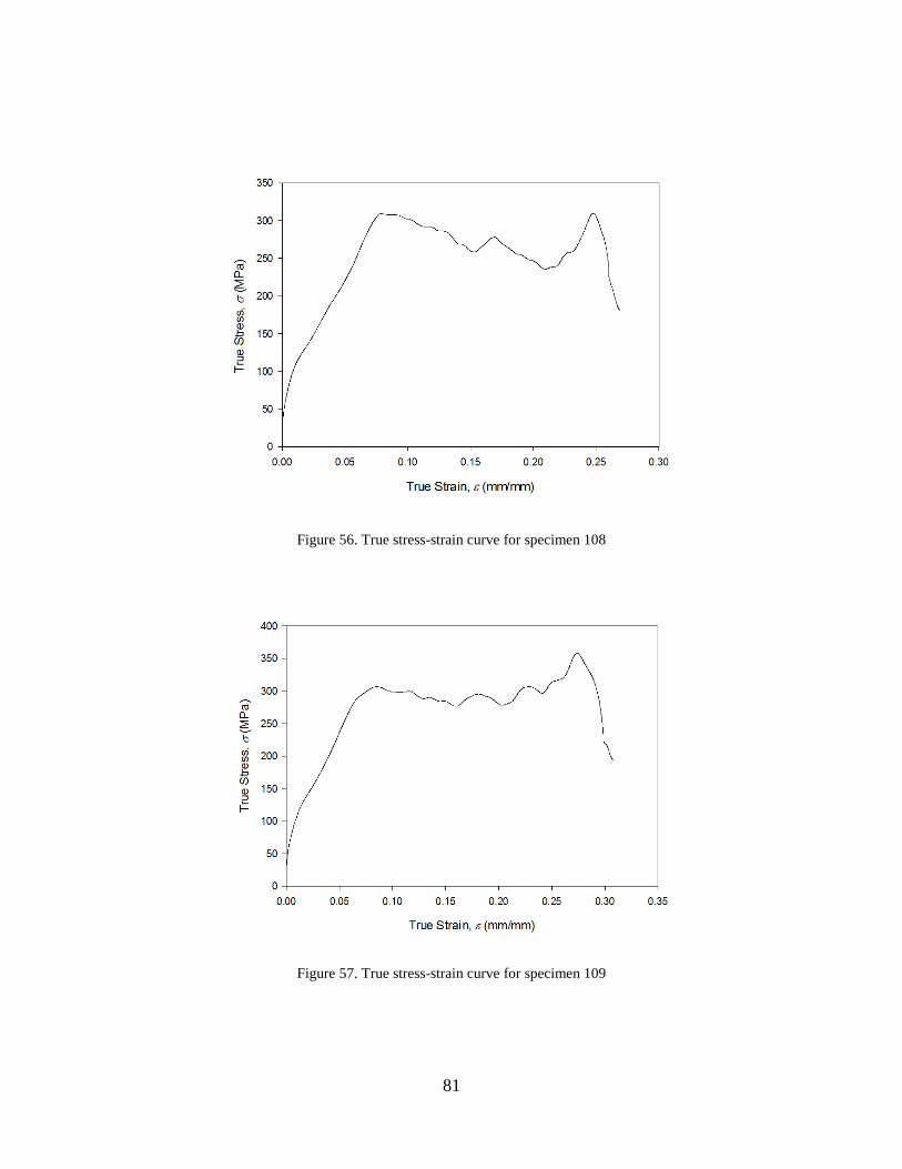
81
Figure 56. True stress-strain curve for specimen 108
Figure 57. True stress-strain curve for specimen 109
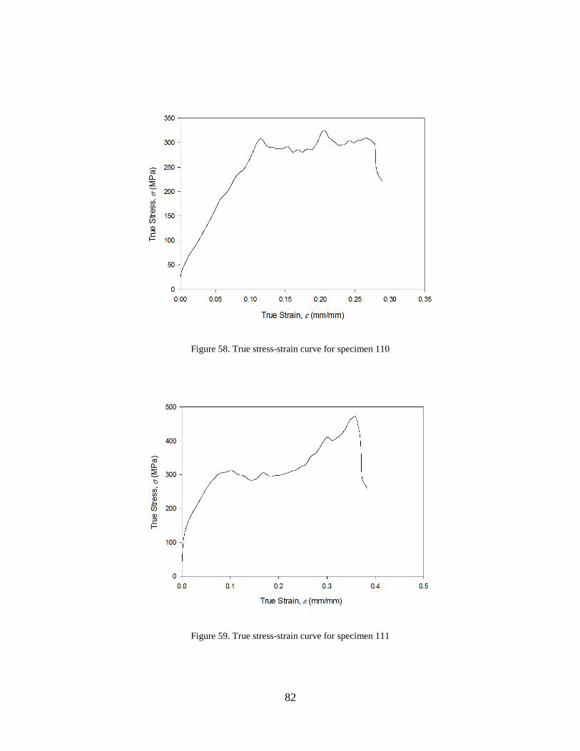
82
Figure 58. True stress-strain curve for specimen 110
Figure 59. True stress-strain curve for specimen 111

83
Figure 60. True stress-strain curve for specimen 112
Figure 61. True stress-strain curve for specimen 113
84
REFERENCES
1. Bauwens Crowet, C. "Tensile Yield-Stress Behaviour of Glassy Polymers." Journal of
polymer science. Part A-2, Polymer physics 7, no. 4 (1969): 735-42.
2. Bijwe, J. "Friction and Wear Studies of Bulk Polyetherimide." Journal of materials
science 25, no. 1 (1990): 548-556.
3. Brown, N.; Ward, I. M. "Load Drop at Upper Yield Point of Polymer." Journal of
Polymer Science A2, no. 6 (1968): 607-620.
4. Chen, W. "A Split Hopkinson Bar Technique for Low-Impedance Materials."
Experimental mechanics 39, no. 2 (1999): 81-5.
5. Chen, Weinong W., Bo Song, and SpringerLink. Split Hopkinson (Kolsky) Bar
[Electronic Resource] : Design, Testing and Applications / Weinong W. Chen, Bo Song
Mechanical Engineering Series. New York: Springer, 2011.
6. Chou, S. C. "The Effect of Strain Rate and Heat Developed During Deformation on the
Stress-Strain Curve of Plastics." Experimental mechanics 13, no. 10 (1973): 422-32.
7. Chree, C. "The Equations of an Isotropic Elastic Solid in Polar and Cylindrical
Coordinates, Their Solutions and Applications." Trans. Cambridge Phios. Soc. 14,
(1889): 251-369.
8. Davies, R. M. "Critical Study of Hopkinson Pressure Bar." Royal Society of London
Philosophical Transactions Series 240, no. 821 (1948): 376-457.
9. Eyring, H. "Viscosity, Plasticity and Diffusion as Examples of Absolute Reaction Rates."
The journal of chemical physics 4, (1936): 283-291.

85
10. Facca, Angelo. "Predicting the Elastic Modulus of Hybrid Fibre Reinforced
Thermoplastics." Polymers & polymer composites 14, no. 3 (2006): 239-250.
11. Field, J. E. "Experimental Methods at High Rates of Strain." Journal de Physique IV
(Colloque) 4, no. 8 (1994): C8-22.
12. Field, J. E. "Review of Experimental Techniques for High Rate Deformation and Shock
Studies." International journal of impact engineering 30, no. 7 (2004): 725-75.
13. Follansbee, P. S. "Wave Propagation in the Split Hopkinson Pressure Bar." Journal of
engineering materials and technology 105, no. 1 (1983): 61-66.
14. Frantz, C. E. "Experimental Techniques with the Split Hopkinson Pressure Bar." In
International Conference on High Energy Rate Fabrication, 229-236, 1984.
15. Gilat, A. "Torsional Split Hopkinson Bar Tests at Strain Rates above 10<Sup>4</Sup>
S(-1)." Experimental mechanics 40, no. 1 (2000): 54-9.
16. Gong, J. C. "Dispersion Investigation in the Split Hopkinson Pressure Bar." Journal of
engineering materials and technology 112, no. 3 (1990): 309-14.
17. Gorham, D. A. "A Numerical Method for the Correction of Dispersion in Pressure Bar
Signals." Journal of physics. E, Scientific instruments 16, no. 6 (1983): 477-9.
18. Gray, G. T. "Influence of Temperature and Strain Rate on the Mechanical Behavior of
Adiprene L-100." Journal de Physique IV (Colloque) 7, no. 3 (1997): 523-8.
19. Gray III, G. T. "Classic Split-Hopkinson Pressure Bar Testing." In A.S.M. Handbook
Volume 8 Mechanical Testing and Evaluation, 463-476: ASM International, 2000.
86
20. Gray III, G. T. and Blumenthal W. R. "Split-Hopkinson Pressure Bar Testing of Soft
Materials." In A.S.M. Handbook Volume 8 Mechanical Testing and Evaluation, 488-496:
ASM International, 2000.
21. Harding, J. "Tensile Testing of Materials at Impact Rates of Strain." Proceedings of the
Institution of Mechanical Engineers; Part C; Journal of Mechanical Engineering Science
2, no. 2 (1960): 88-96.
22. Hopkinson, B. "A Method of Measuring the Pressure Produced in the Detonation of High
Explosives or by the Impact of Bullets." Philosophical Transactions of the Royal Society
of London 213, (1914): 19.
23. Jia, D. "A Rigorous Assessment of the Benefits of Miniaturization in the Kolsky Bar
System." Experimental mechanics 44, no. 5 (2004): 445-54.
24. Klepaczko, J. Application of the Split Hopkinson Pressure Bar to Fracture Dynamics
25. Mechanical Properties at High Rates of Strain, 1979, 1980.
26. Kolsky, H. "An Investigation of the Mechanical Properties of Materials at Very High
Rates of Loading." Proceedings of the Physical Society 62, (1949): 676-700.
27. Lewis, J. L. "A Biaxial Split Hopkinson Bar for Simultaneous Torsion and
Compression." Review of scientific instruments 44, no. 7 (1973): 811-13.
28. Lifshitz, J. M. "Data Processing in the Split Hopkinson Pressure Bar Tests." International
journal of impact engineering 15, no. 6 (1994): 723-733.
29. Lili, Wang. "Generalization of Split Hopkinson Bar Technique to Use Viscoelastic Bars."
International journal of impact engineering 15, no. 5 (1994): 669-86.

87
30. Marshall, I. "Drawing of `Terylene'." Journal of applied chemistry 4, no. 4 (1954): 145-
153.
31. Nemat Nasser, S. "Hopkinson Techniques for Dynamic Recovery Experiments."
Proceedings of the Royal Society of London. Series A, Mathematical and physical
sciences 435, no. 1894 (1991): 371-91.
32. Nemat-Nasser, S.; Isaacs, J.; Rome, J. "Triaxial Hopkinson Techniques." In A.S.M.
Handbook Volume 8 Mechanical Testing and Evaluation, 516-518: ASM International,
2000.
33. Nicholas, T. "Tensile Testing of Materials at High Rates of Strain." Experimental
mechanics 21, no. 5 (1981): 177-85.
34. Pecht, M. Characterization of Polyimides Used in Ge High Density Interconnects [Mcm
Packaging]
35. Proceeding Sampe 7th International Electronic Materials and Processes Conference,
1994.
36. Pochhammer, L. "Uber Fortplanzungsgeschwindigkeiten Kleiner Schwingungen in
Einem Unbergrenzten Isotropen Kreiszlinder." J. Reinge Angew. Math 81, no. 234
(1876).
37. Ree, T. "Theory Non-Newtonian Flow. Ii. Solution System of High Polymers." Journal of
applied physics 26, no. 7 (1955): 800-809.
38. Sawas, O. "Dynamic Characterization of Compliant Materials Using an All-Polymeric
Split Hopkinson Bar." Experimental mechanics 38, no. 3 (1998): 204-10.

88
39. Siviour, C. R. "The High Strain Rate Compressive Behaviour of Polycarbonate and
Polyvinylidene Difluoride." Polymer 46, no. 26 (2005): 12546-55.
40. Smmaz, and Tamer elik. "The Effects of Thermal Cycles on the Impact Fatigue
Properties of Thermoplastic Matrix Composites." Applied composite materials 15, no. 2
(2008): 99-113.
41. Staab, G. H. "Direct-Tension Split Hopkinson Bar for High Strain-Rate Testing."
Experimental mechanics 31, no. 3 (1991): 232-235.
42. Stokes, Vijay. "Lateral Strain Effects During the Large Extension of Thermoplastics."
Polymer engineering and science 28, no. 19 (1988): 1209-1218.
43. Subhash, G. and Ravichandran, G. "Split-Hopkinson Pressure Bar Testing of Ceramics."
In A.S.M. Handbook Volume 8 Mechanical Testing and Evaluation, 497-504: ASM
International, 2000.
44. Tou, G.; Sihui, X. "Mean Stress/Strain Effect on Fatigue Behavior of an Epoxy Resin."
International journal of fatigue 29, no. 12 (2007): 2180-2190.
45. Tyas, A. "Full Correction of First-Mode Pochammer-Chree Dispersion Effects in
Experimental Pressure Bar Signals." Measurement science & technology 16, no. 3
(2005): 642-52.
46. Vincent, P. I. Polymer 1, (1960).
47. Walley, S. M. "A Study of the Rapid Deformation Behaviour of a Range of Polymers."
Philosophical Transactions of the Royal Society of London, Series A: Mathematical and
Physical Sciences 328, no. 1597 (1989): 1-33.

89
48. Walley, S. M. "A Comparison of the High Strain Rate Behaviour in Compression of
Polymers at 300 K and 100 K." Journal de Physique IV (Colloque) 1, no. 3 (1991): 185-
90.
49. Walley, S. M. "The Rapid Deformation Behaviour of Various Polymers." Journal de
physique. III 1, no. 12 (1991): 1889-925.
50. Wang, Lili. "Generalization of Split Hopkinson Bar Technique to Use Viscoelastic Bars."
International journal of impact engineering 15, no. 5 (1994): 669-686.
51. Yew, E. H. "Experimental Study of Dispersive Waves in Beam and Rod Using Fft."
Journal of applied mechanics 45, no. 4 (1978): 940-2.
52. Zhao, H. "On the Use of a Viscoelastic Split Hopkinson Pressure Bar." International
journal of impact engineering 19, no. 4 (1997): 319-30.
53. Zhao, Han. "Study on Testing Techniques for Concrete-Like Materials under
Compressive Impact Loading." Cement & concrete composites 20, no. 4 (1998): 293-
299.